Embed Size (px)
Citation preview
Module 5 – Calculus
Module 5
CALCULUS 5
Table of Contents A – Differentiation .......................................................................................................... 5.1
Derivatives ...................................................................................................................... 5.1 Finding Derivatives from First Principles ................................................................... 5.2
Gradient Functions ......................................................................................................... 5.3
Differentiability .............................................................................................................. 5.5
Derivatives of Simple Functions .................................................................................... 5.8
Practical Interpretations of the Derivative ...................................................................... 5.11
Simple Applications of the Derivative ........................................................................... 5.12
The Product Rule ............................................................................................................ 5.15
The Quotient Rule .......................................................................................................... 5.17
The Chain Rule ............................................................................................................... 5.21
Stationary Points ............................................................................................................. 5.29 Second Derivatives ..................................................................................................... 5.32 Identifying Stationary Points Using the Second Derivative Test ............................... 5.39
Curve Sketching ............................................................................................................. 5.43
Maximum/Minimum Problems ...................................................................................... 5.48
Newton-Raphson Method for Finding Roots ................................................................. 5.53
Solutions to Exercise Sets ............................................................................................... 5.60

Module 5 – Calculus 5.1
A – Differentiation
Module 4 – Trigonometry
From your earlier studies in 11083 or its equivalent or at school you have been introduced to differential calculus. Differential calculus is about the rate of change of one variable with respect to another variable. The typical examples you have probably met are, velocity as the rate of change of position with respect to time, and acceleration as the rate of change of velocity with respect to time. Here is a brief revision of derivatives, gradient functions and differentiation of simple functions. These topics are assumed knowledge in this unit.
Derivatives
We often talk about the average velocity for a trip. For example, if it takes 6 hours to travel 480 kilometres we say that the average velocity was 80 kilometres per hour. Obviously the velocity of the trip was not 80 km h–1 every instant of the journey. We could get reasonable estimates of the velocity for each half-hour of the trip by finding the change in distance travelled and hence calculating the average speed in km h–1 for each half-hour. We could the note the distance travelled each 5 minutes of the trip and calculate the velocity in km h–1 for each 5 minutes of the trip. If the relationship between position, s and time, t, is given by the function s(t) we can write
See Note 1
average velocity = = See Note 2
As s = s(t) we can express the change in position as s(t2) – s(t1), where t2 – t1 is the elapsed time.
If we then let t2 – t1 = h, we can write
average velocity = =
By continuing to make the elapsed time smaller and smaller we can get closer and closer to the velocity at any instant. We then write the instantaneous velocity as the derivative
= v(t) = See Note 3
If you need refreshment on limits go back to module 2.
Notes
1. s(t) is read as “s is a function of t”.
2. is the Greek capital letter delta. s is read as “delta s”, and means a small change in s ; t is read as “delta t”, and
means a small change in t.
3. is read as “dee s dee t” which sometimes causes confusion. If you like you could read it as “dee s on dee t”.
change in position
elapsed time--------------------------------------------
s
t------
s
t------
s t h+! " s t! "–
h---------------------------------
ds
dt-----
h 0#lim
s t h+! " s t! "–
h---------------------------------
ds
dt-----

5.2 TPP7184 – Mathematics Tertiary Preparation Level D
Similarly the definition of instantaneous acceleration, a, is derived from the change in velocity with respect to time:
= a(t) =
For any function y = f(x), the derivative of y with respect to x is given by
=
Another notation for the derivative of y with respect to x, where y = f(x) is . See Note 1
Finding Derivatives from First Principles
In this level of mathematics you will be expected to be able to use the definition of the derivative as a limit to find the gradient function for simple functions. This is called finding the derivative from first principles.
We can find the derivative of any function y = f(x), from first principles using
(Sometimes the calculations are quite difficult)
You need good algebraic skills and a solid understanding of functions to find derivatives from first principles. If necessary revise module 2 before proceeding.Example 5.1:
Find the derivative of f(x) = 3x2
Solution:
=
=
=
=
Notes
1. is read as “f dash x” and means .
dv
dt------
h 0#lim
v t h+! " v t! "–
h----------------------------------
dy
dx------
h 0#lim
f x h+! " f x! "–
h----------------------------------
f ' x! "
f ' x! "d f
dx------
df
dx------
h 0#lim
f x h+! " f x! "–
h----------------------------------=
df
dx------
h 0#lim
f x h+! " f x! "–
h----------------------------------
h 0#lim
3 x h+! "2 3x2
–
h-------------------------------------
h 0#lim
3 x2
2hx h2
+ +! " 3x2
–
h-------------------------------------------------------
h 0#lim
3x2
6hx 3h2
3x2
–+ +
h-----------------------------------------------------
Module 5 – Calculus 5.3
=
=
= 6x + 3h
= 6x {As h gets closer and closer to zero, 3h gets closer to zero}
We could now find the derivative of f(x) = 3x2 for any value of x.
e.g when x = 3, = 6x = 6 $ 3 = 18
when x = 0, = 6 $ 0 = 0
when x = , = 6 $ = –9
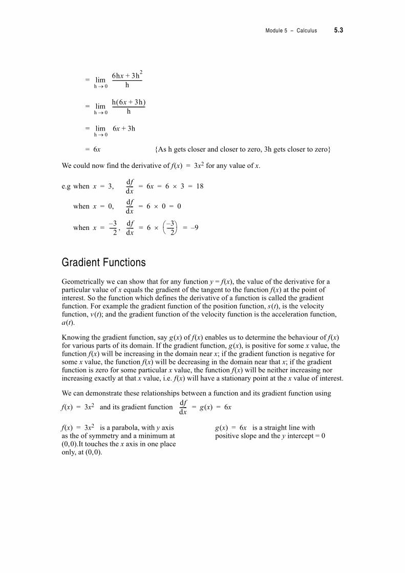
Gradient Functions
Geometrically we can show that for any function y = f(x), the value of the derivative for a particular value of x equals the gradient of the tangent to the function f(x) at the point of interest. So the function which defines the derivative of a function is called the gradient function. For example the gradient function of the position function, s(t), is the velocity function, v(t); and the gradient function of the velocity function is the acceleration function, a(t).
Knowing the gradient function, say g(x) of f(x) enables us to determine the behaviour of f(x) for various parts of its domain. If the gradient function, g(x), is positive for some x value, the function f(x) will be increasing in the domain near x; if the gradient function is negative for some x value, the function f(x) will be decreasing in the domain near that x; if the gradient function is zero for some particular x value, the function f(x) will be neither increasing nor increasing exactly at that x value, i.e. f(x) will have a stationary point at the x value of interest.
We can demonstrate these relationships between a function and its gradient function using
f(x) = 3x2 and its gradient function = g(x) = 6x
f(x) = 3x2 is a parabola, with y axis g(x) = 6x is a straight line with as the of symmetry and a minimum at positive slope and the y intercept = 0(0,0).It touches the x axis in one place only, at (0,0).
h 0#lim
6hx 3h2
+
h------------------------
h 6x 3h+! "h
--------------------------h 0#lim
h 0#lim
df
dx------
df
dx------
3–
2------
df
dx------
3–
2------% &' (
df
dx------

5.4 TPP7184 – Mathematics Tertiary Preparation Level D
We’ve already shown that when x = 3, = 18.
Check the graph of f(x) = 3x2. How is it behaving near x = 3? . . . . . . . . . . . . . . . . . . . . . .
. . . . . . . . . . . . . . . . . . . . . . . . . . . . . . . . . . . . . . . . . . . . . . . . . . . . . . . . . . . . . . . . . . . . . . . . . . .
Answer:
It’s rising steeply, i.e. it is increasing.
Check the value of when x = 3. Is it positive and relatively large? . . . . . . . . . . . . . . . . .
. . . . . . . . . . . . . . . . . . . . . . . . . . . . . . . . . . . . . . . . . . . . . . . . . . . . . . . . . . . . . . . . . . . . . . . . . . .
Answer:
Yes, because the gradient function g(x) = 6x indicates the behaviour of f(x) = 3x2 in terms of where it is increasing or decreasing .
If we check the behaviour of f(x) = 3x2 at other values of x and the value of the gradient function at each respective x value we see that the gradient function g(x) = 6x always tells us how the function f(x) = 3x2 behaves.
e.g. when x = 0, = 6x = 0 because f(x) = 3x2 is neither increasing nor decreasing. It
is at a stationary point. In this case, the stationary point is a turning point.
e.g. when x = , = 6x = –9 because near x = , f(x) = 3x2 is decreasing
but not as ‘steeply’ as say at x = –3 or x = –10.
x
y
df
dx------
df
dx------
df
dx------
3–
2------
df
dx------
3–
2------

Module 5 – Calculus 5.5
Differentiability
Not all functions are differentiable across their domains because
• either they are discontinuous at some value of x,
e.g. f(x) = is not differentiable at x = 2
• or the function is continuous for some value of x but the limit as h # 0 of the quotient
does not exist because a corner occurs at x.
e.g. is not differentiable at x = 0 because the
is not the same if you approach x = 0 from the left and the right. From the left,
and from the right,
Recall from module 2 that for the limit at some value of x, say a, to exist the following conditions must apply:
• the limit as x approaches a from the positive side exists
• and is the same as the limit as x approaches a from the negative side
• and the value of the limit is the same as the functional value of x at the point a.
Check back to module 2 for some examples of functions that do not have limits or are not continuous at certain values of x.
1
x 2–-----------
f x h+! " f x! "–
h----------------------------------
f x! " x=h 0#lim
f x h+! " f x! "–
h----------------------------------
df x! "dx
------------d x–! "
dx-------------- 1–= =
df x! "dx
------------d x! "dx
---------- 1= =
5.6 TPP7184 – Mathematics Tertiary Preparation Level D
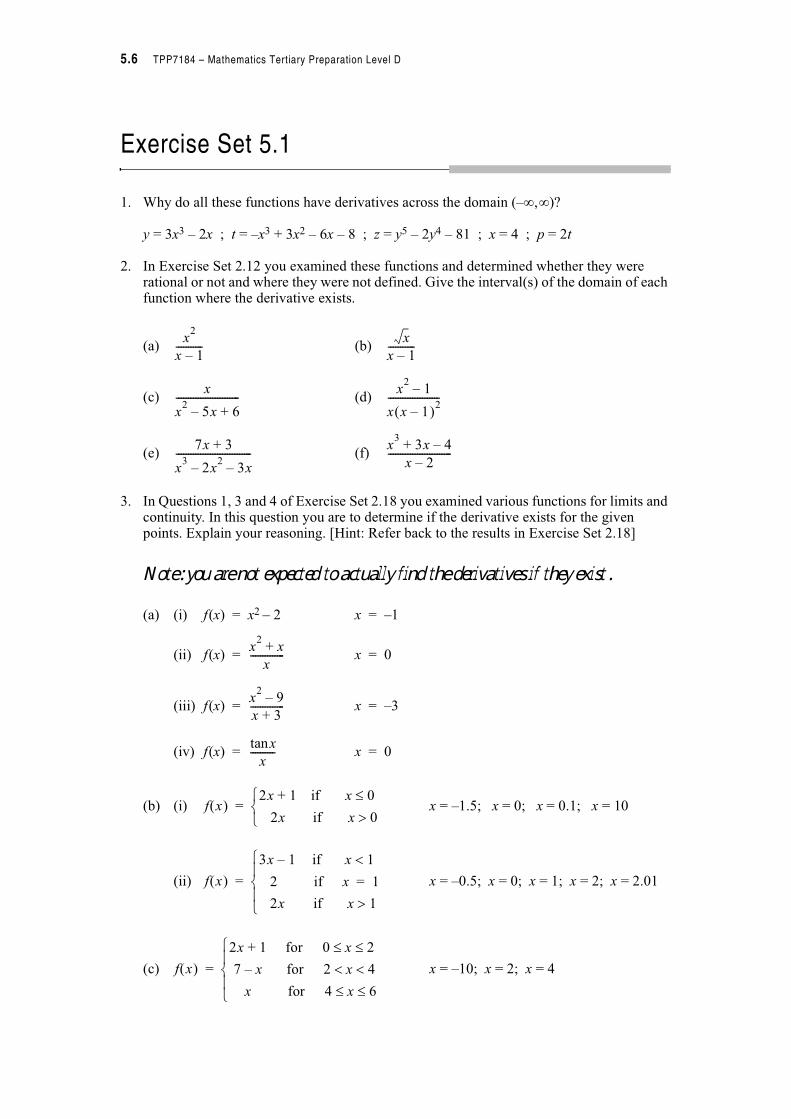
Exercise Set 5.1
1. Why do all these functions have derivatives across the domain (–),))?
y = 3x3 – 2x ; t = –x3 + 3x2 – 6x – 8 ; z = y5 – 2y4 – 81 ; x = 4 ; p = 2t
2. In Exercise Set 2.12 you examined these functions and determined whether they were rational or not and where they were not defined. Give the interval(s) of the domain of each function where the derivative exists.
(a) (b)
(c) (d)
(e) (f)
3. In Questions 1, 3 and 4 of Exercise Set 2.18 you examined various functions for limits and continuity. In this question you are to determine if the derivative exists for the given points. Explain your reasoning. [Hint: Refer back to the results in Exercise Set 2.18]
Note: you are not expected to actually find the derivatives if they exist.(a) (i) f(x) = x2 – 2 x = –1
(ii) f(x) = x = 0
(iii) f(x) = x = –3
(iv) f(x) = x = 0
(b) (i) x = –1.5; x = 0; x = 0.1; x = 10
(ii) x = –0.5; x = 0; x = 1; x = 2; x = 2.01
(c) x = –10; x = 2; x = 4
x2
x 1–-----------
x
x 1–-----------
x
x2
5x– 6+--------------------------
x2
1–
x x 1–! "2---------------------
7x 3+
x3
2x2
– 3x–-------------------------------
x3
3x 4–+
x 2–--------------------------
x2
x+
x--------------
x2
9–
x 3+--------------
xtan
x----------
f x! "2x 1+ if x 0*
2x if x 0+,-.
=
f x! "
3x 1– if x 1/
2 if x 1=
2x if x 1+,0-0.
=
f x! "
2x 1+ for 0 x 2* *
7 x– for 2 x 4/ /
x for 4 x 6* *,0-0.
=
Module 5 – Calculus 5.7
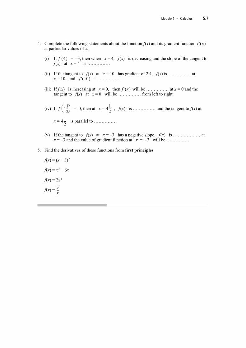
4. Complete the following statements about the function f(x) and its gradient function at particular values of x.
(i) If = –3, then when x = 4, f(x) is decreasing and the slope of the tangent to f(x) at x = 4 is ……………
(ii) If the tangent to f(x) at x = 10 has gradient of 2.4, f(x) is …………… at x = 10 and = ……………
(iii) If f(x) is increasing at x = 0, then will be …………… at x = 0 and the tangent to f(x) at x = 0 will be …………… from left to right.
(iv) If = 0, then at x = , f(x) is …………… and the tangent to f(x) at
x = is parallel to ……………
(v) If the tangent to f(x) at x = –3 has a negative slope, f(x) is ……………… atx = –3 and the value of gradient function at x = –3 will be ……………
5. Find the derivatives of these functions from first principles.
f(x) = (x + 3)2
f(x) = x2 + 6x
f(x) = 2x3
f(x) =
f ' x! "
f ' 4! "
f ' 10! "
f ' x! "
f ' 41
2---% &
' ( 41
2---
41
2---
3
x---

5.8 TPP7184 – Mathematics Tertiary Preparation Level D
Derivatives of Simple Functions
You have previously met the derivatives of the functions shown in the table below. If you are not convinced that the gradient functions given are correct,
• either choose a typical example f(x), of each type of function and find the derivative from first principles (if you can), and compare the result with the relevant formula from the table • or graph your original function f(x) and identify the regions of the domain of x where f(x) is increasing; where f(x) is decreasing and where there is a stationary point and then draw a rough sketch of the gradient function you expect and compare it with the graph of the gradient function given by the formula.
Note:
• The only function that has its functional values the same as its derivative values isf(x) = ex.
• The functions x, and are special cases of xn with n = 1, and –1
respectively. They are such common functions that for your convenience you should know
them ‘off by heart’.
Function, f(x) Derivative or Gradient Function,
any constant, e.g. c
a variable raised to a power, e.g. xn
a constant multiplied by a power of x, e.g. a.u(x)
the sum or difference of two functions
e.g. u(x) + v(x)
u(x) – v(x)
sin x
cos x
ex
ln x
0
n.xn–1
a. (where a is a constant)
+
–
cos x
–sin x
ex
Function, f(x) Derivative or Gradient Function,
x
or
or x–1
1
or
or
f ' x! "
u ' x! "
u ' x! " v ' x! "
u ' x! " v ' x! "
1
x---
x1
x---
1
2---
f ' x! "
x x
1
2---
1
x---
1
2 x----------
1
2---x
1
2---–
1
x2
-----– x2–
–
Module 5 – Calculus 5.9
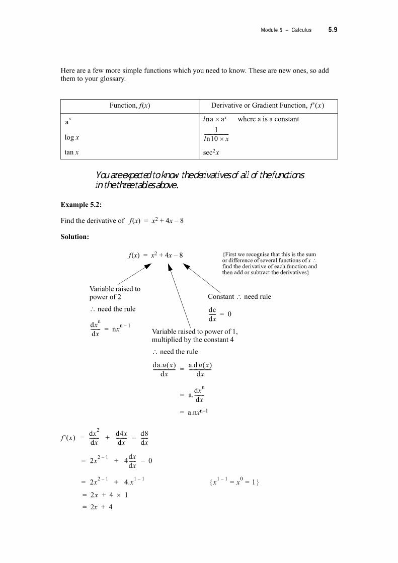
Here are a few more simple functions which you need to know. These are new ones, so add them to your glossary.
You are expected to know the derivatives of all of the functions in the three tables above.Example 5.2:
Find the derivative of f(x) = x2 + 4x – 8
Solution:
= –
= – 0
=
= 2x + 4 $ 1
= 2x + 4
Function, f(x) Derivative or Gradient Function,
log x
tan x
lna $ ax where a is a constant
sec2x
f ' x! "
ax
1
ln10 x$--------------------
Variable raised to power of 2
1 need the rule
dxn
dx-------- nx
n 1–= Variable raised to power of 1,
multiplied by the constant 4
1 need the rule
=
=
= a.nxn–1
da.u x! "dx
------------------a.d u x! "
dx------------------
a.dx
n
dx--------
Constant212need rule
dc
dx------ 0=
{First we recognise that this is the sum or difference of several functions of x 1 find the derivative of each function and then add or subtract the derivatives}
f(x) = x2 + 4x – 8
f ' x! "dx
2
dx--------
d4x
dx---------+
d8
dx------
2x2 1–
4dx
dx------+
2x2 1–
4.x1 1–
+ x1 1–
x0
1= =3 4
5.10 TPP7184 – Mathematics Tertiary Preparation Level D
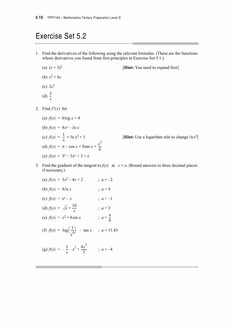
Exercise Set 5.2
1. Find the derivatives of the following using the relevant formulae. (These are the functions whose derivatives you found from first principles in Exercise Set 5.1.)
(a) (x + 3)2 [Hint: You need to expand first]
(b) x2 + 6x
(c) 2x3
(d)
2. Find for
(a) f(x) = 6log x + 4
(b) f(x) = 8ex – ln x
(c) f(x) = + ln x2 + 1 [Hint: Use a logarithm rule to change lnx2]
(d) f(x) = 5 – cos x + 8tan x +
(e) f(x) = 3x – 3ex + 3 + e
3. Find the gradient of the tangent to f(x) at x = a. (Round answers to three decimal places if necessary.)
(a) f(x) = 3x2 – 4x + 2 ; a = –2
(b) f(x) = 8ln x ; a = 4
(c) f(x) = ex – x ; a = –1
(d) f(x) = ; a = 3
(e) f(x) = x2 + 6sin x ; a =
(f) f(x) = – tan x ; a = 11.43
(g) f(x) = ; a = –4
3
x---
f ' x! "
1
x---
x2
6-----
x10
x------+
56---
1
x6
-----% &' (log
1
x---– x
2–
4x3
3--------+
Module 5 – Calculus 5.11
Practical Interpretations of the Derivative
Problems involving derivatives always involve quantities or measurements where the unit of measurement is ‘something’ per ‘something’. Examination of the unit of measurement will help you identify the derivatives of interest. For example
• cost of building a house, C, is a function of the floor area of the house, A
i.e. C = C(A)
So will have the unit $ per m2
• population, P is a function of time, t
i.e. P = P(t)
So will have the unit number of people per year
• income, I, is a function of the amount spent on advertising, a
i.e. I = I(a)
So will have the unit $income per $advertising
• radiation level, R, is a function of time since accident, t
i.e. R = R(t)
So will have the unit millirems per hour
Let’s look at one example which shows how the derivative can be used in real life.
The size of a bacterial population, P, is a function of time, t, (measured in hours), i.e. P = P(t).
If = –8 000 when t = 1, what does this mean in real life?
This derivative tell us that at exactly one hour after measurement began the population was declining by 8 000 bacteria per hour. Practically, this means we should expect about 8 000 less bacteria to be present at the second hour than at the first hour. Note that you would not expect
there to be exactly 8 000 less bacteria at the second hour because the rate, at t = 1 will be
different to the rate at t = 1.01 hours, or t = 1.1 hours, or t = 1.5 hours, etc.
Before we move on to some new rules for differentiation, which will enable us to solve many interesting and quite complicated problems, we will spend a short time solving a few problems which require only the rules on pages 5.8 and 5.9.
C ' A !dC
dA-------=
P ' t !dP
dt-------=
I ' a !dI
da------=
R ' t !dR
dt-------=
dP
dt-------
dP
dt-------
dP
dt-------

5.12 TPP7184 – Mathematics Tertiary Preparation Level D
Simple Applications of the Derivative
When solving any problem there are a few basic techniques which most people find helpful. (You may care to look up the section on ‘Hints for Success in Mathematics Learning’ in the Introductory Book for this unit for some more ideas.)
Here’s a general approach demonstrated by means of an example.
Example 5.3:
Sand falling from a chute into a shed forms a conical pile whose vertical height is always equal to the radius of the base. Find the rate of change of volume with respect to height when the height is 20 m.
Solution:
STEP 1: Draw a picture
STEP 2: Write down the derivative required from the rate of change specified.
Rate of change of volume, V, with respect to height, h, is required
i.e. is needed.
STEP 3: Look for a relationship between the variables in the derivative, (usually, this is a formula.) This will be the principal equation.
Relationship between V and h is needed.
Volume of a cone, V =
STEP 4: Check if this formula involves another variable. If it does, look for a relationship between this extra variable and the variable in the denominator of the derivative. Find an auxiliary equation so a substitution can be made in order that only two variables remain in the principal equation.
RHS of principal equation has r and h as variables. We need to eliminate r. Look for a relationship between r and h. In this case h = r is the auxiliary equation.
" V =
becomes V = i.e. V = V(h)
dV
dh-------
1
3---#r
2h
1
3---#h
2h
1
3---#h
3

Module 5 – Calculus 5.13
STEP 5: Differentiate using the appropriate rules. Check the unit of measurement of the derivative from the units of the variables involved. (Do a dimension analysis.) Make sure the unit of the derivative makes sense.
STEP 6: Look at the derivative for extreme values of the independent variable and make sure it makes sense for such values.
When h is zero, = 0 (no height $ no pile ✓ )
When h is very large, % & (no limit on pile, as the height gets bigger the volume increases. ✓ )
STEP 7: Evaluate the derivative for the specified conditions
When h = 20 m
= #h2
= # ' 202
= 1 257 m3 per m.
STEP 8: Express your answer in a sentence.
When the pile is 20 m high its volume is increasing at the rate of 1 257 cubic metres per metre of height increase.
Dimension Analysis
V = m3 ; h = m
= (m3 per m)
and #h2 has units m2 ✓
dV
dh-------
m3
m-------=
m3
m--------
( )* +, -
m2
=
= #h2
dV
dh-------
1
3---# 3 h
2''=
dV
dh-------
dV
dh-------
dV
dh-------
5.14 TPP7184 – Mathematics Tertiary Preparation Level D
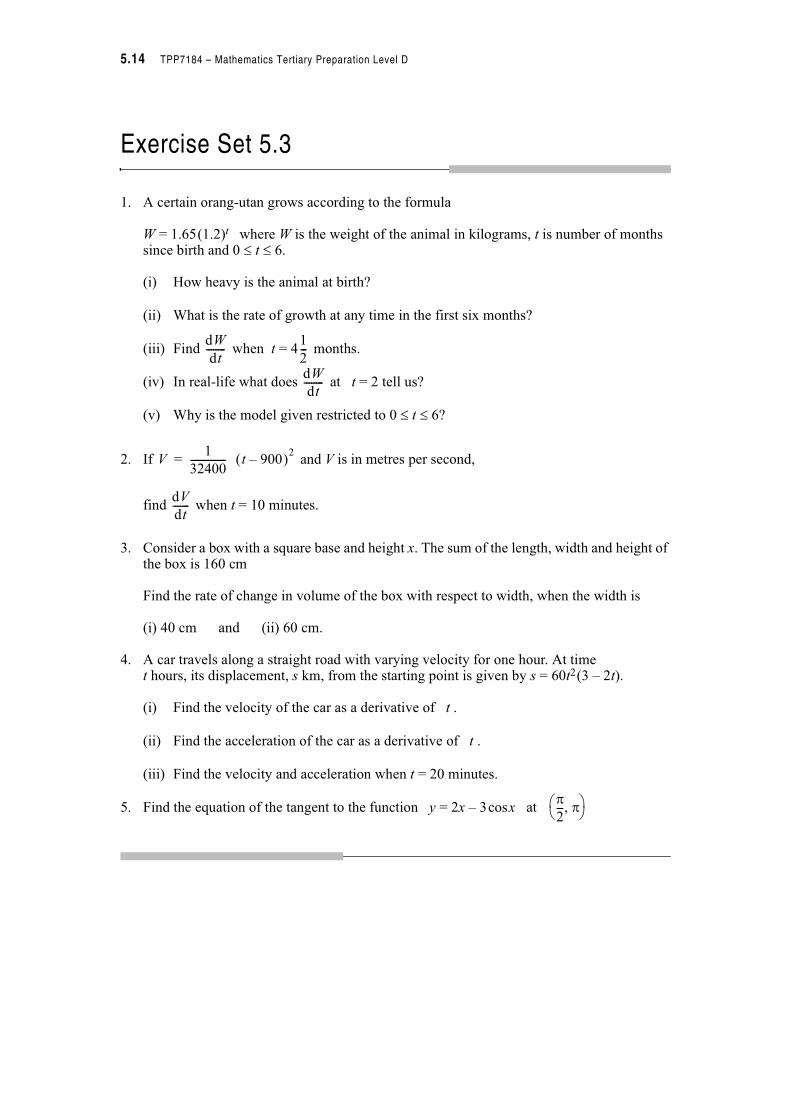
Exercise Set 5.3
1. A certain orang-utan grows according to the formula
W = 1.65(1.2)t where W is the weight of the animal in kilograms, t is number of months since birth and 0 . t . 6.
(i) How heavy is the animal at birth?
(ii) What is the rate of growth at any time in the first six months?
(iii) Find when t = 4 months.
(iv) In real-life what does at t = 2 tell us?
(v) Why is the model given restricted to 0 ./t . 6?
2. If and V is in metres per second,
find when t = 10 minutes.
3. Consider a box with a square base and height x. The sum of the length, width and height of the box is 160 cm
Find the rate of change in volume of the box with respect to width, when the width is
(i) 40 cm and (ii) 60 cm.
4. A car travels along a straight road with varying velocity for one hour. At time t hours, its displacement, s km, from the starting point is given by s = 60t2(3 – 2t).
(i) Find the velocity of the car as a derivative of t .
(ii) Find the acceleration of the car as a derivative of t .
(iii) Find the velocity and acceleration when t = 20 minutes.
5. Find the equation of the tangent to the function y = 2x – 3cosx at
dW
dt--------
1
2---
dW
dt--------
V1
32400--------------- t 900– !2
=
dV
dt-------
#2--- #0( )
, -

Module 5 – Calculus 5.15
You already know how to find derivatives of functions which are constants (e.g. 4.6), powers
(e.g. x3), exponentials (e.g. ex), logarithms (e.g. log x), trigonometric functions (e.g. sin x) and
sums or differences or multiples of these, (e.g. 10 + 3x + 2lnx – 8 – tan x)
Now we move on to more complicated functions such as sin(ln x), ex .cos x, etc.
There are three new rules you need to know to be able to handle such functions These are the product rule, the quotient rule, and the chain rule. See Note 1
The Product Rule
Consider the function y = f(x) = 3x2cosx. This function is the product of two functions of x, namely 3x2 and cos x.
We will let u(x) = 3x2 and v(x) = cos x then y = f(x) = u(x) . v(x).
Following on from the notion of the derivative being a limit, let a small change in x, say 1x, result in a small change in u, say 1u, and a small change in v, say 1v See Note 2
i.e. f(x + 1x) = (u + 1u) . (v + 1v)
= u . v + u . 1v + 1u . v + 1u . 1v {using the distributive law}
Now the actual change in the functional value will be
1y = f(x + 1x) – f(x)
Therefore 1y = (u . v + u . 1v + 1u . v + 1u . 1v) – u.v
i.e. 1y = u . 1v + v . 1u + 1u . 1v
Dividing through by 1x yields:
= + +
Then if we let 1x get smaller and smaller we get closer and closer to the derivative of y = f(x) = u(x) . v(x)
+ +
Thus at the limit,
+ product rule
Notes
1. The chain rule is also known as the function of a function rule.
2. Recall the formula for finding the derivative of a simple function from first principles.
1
2---
3x 2–
8x lnx 4+–-----------------------------
1y
1x------ u
1v
1x------2 v
1u
1x-------2 1u
1v
1x------2
dy
dx------
1x 0%lim
f x 1x+ ! f x !–
1x--------------------------------------
1x 0%lim= = u
1v
1x------2 v
1u
1x-------2 1u
1v
1x------2
dy
dx------
du x ! v x !2dx
----------------------------- udv
dx------2= = v
du
dx------2
5.16 TPP7184 – Mathematics Tertiary Preparation Level D
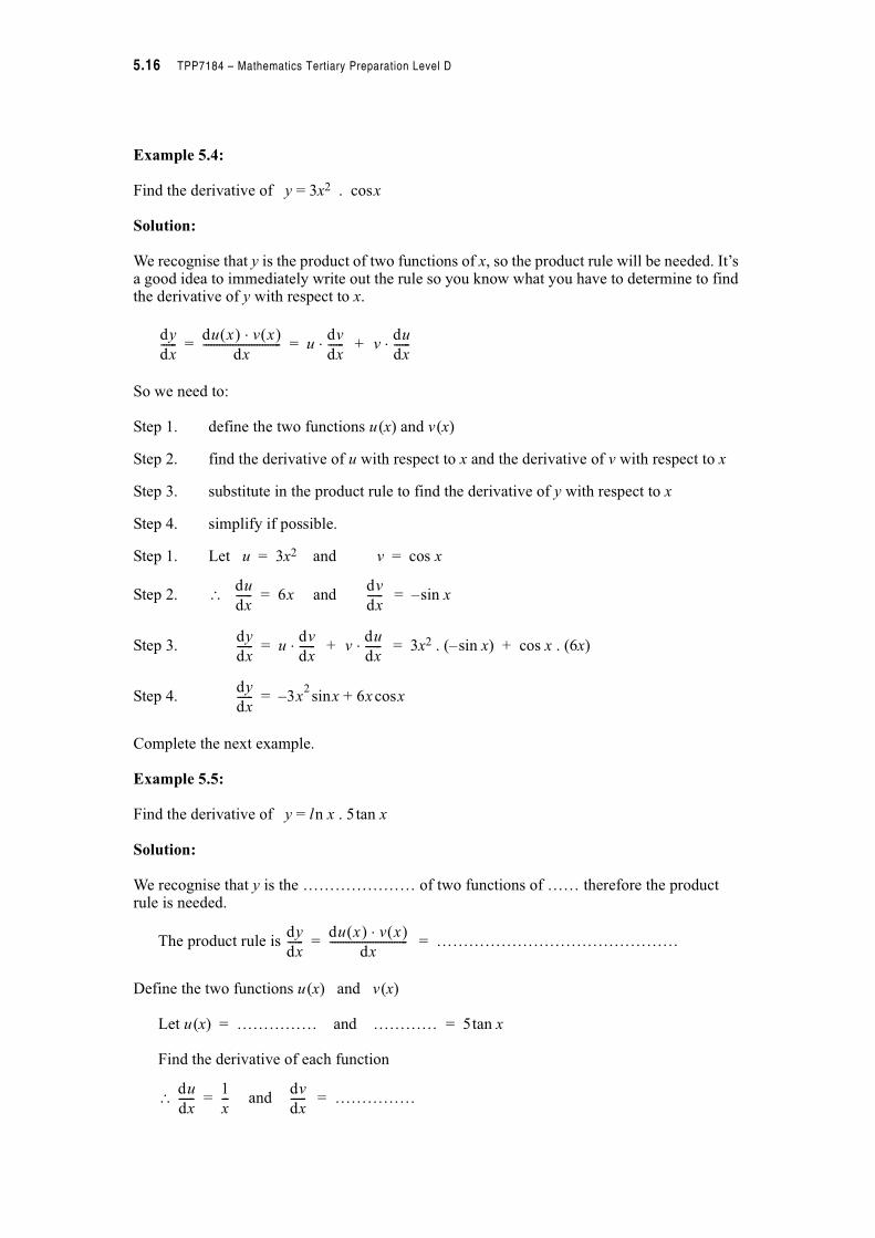
Example 5.4:
Find the derivative of y = 3x2 . cosx
Solution:
We recognise that y is the product of two functions of x, so the product rule will be needed. It’s a good idea to immediately write out the rule so you know what you have to determine to find the derivative of y with respect to x.
+
So we need to:
Step 1. define the two functions u(x) and v(x)
Step 2. find the derivative of u with respect to x and the derivative of v with respect to x
Step 3. substitute in the product rule to find the derivative of y with respect to x
Step 4. simplify if possible.
Step 1. Let u = 3x2 and v = cos x
Step 2. " and = –sin x
Step 3. + = 3x2 . (–sin x) + cos x . (6x)
Step 4.
Complete the next example.
Example 5.5:
Find the derivative of y = ln x . 5tan x
Solution:
We recognise that y is the ………………… of two functions of …… therefore the product rule is needed.
The product rule is = ………………………………………
Define the two functions u(x) and v(x)
Let u(x) = …………… and ………… = 5tan x
Find the derivative of each function
" and = ……………
dy
dx------
du x ! v x !2dx
----------------------------- udv
dx------2= = v
du
dx------2
du
dx------ 6x=
dv
dx------
dy
dx------ u
dv
dx------2= v
du
dx------2
dy
dx------ 3x
2xsin 6x xcos+–=
dy
dx------
du x ! v x !2dx
-----------------------------=
du
dx------
1
x---=
dv
dx------
Module 5 – Calculus 5.17
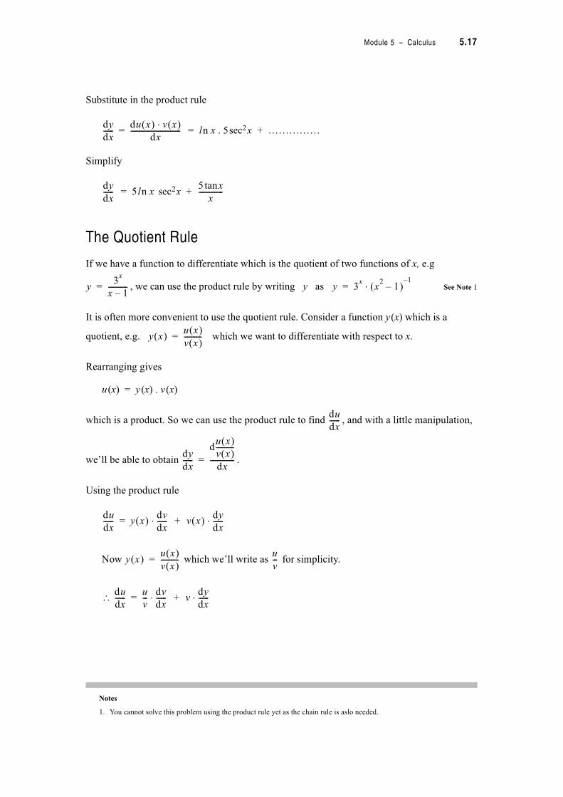
Substitute in the product rule
= ln x . 5sec2x + ……………
Simplify
= 5ln x sec2x +
The Quotient Rule
If we have a function to differentiate which is the quotient of two functions of x, e.g
, we can use the product rule by writing y as See Note 1
It is often more convenient to use the quotient rule. Consider a function y(x) which is a
quotient, e.g. which we want to differentiate with respect to x.
Rearranging gives
u(x) = y(x) . v(x)
which is a product. So we can use the product rule to find , and with a little manipulation,
we’ll be able to obtain .
Using the product rule
+
Now which we’ll write as for simplicity.
" +
Notes
1. You cannot solve this problem using the product rule yet as the chain rule is aslo needed.
dy
dx------
du x ! v x !2dx
-----------------------------=
dy
dx------
5 xtan
x--------------
y3
x
x 1–-----------= y 3
xx
21– !
1–2=
y x !u x !v x !----------=
du
dx------
dy
dx------
du x !v x !----------
dx--------------=
du
dx------ y x !
dv
dx------2= v x !
dy
dx------2
y x !u x !v x !----------=
u
v---
du
dx------
u
v---
dv
dx------2= v
dy
dx------2
5.18 TPP7184 – Mathematics Tertiary Preparation Level D
Now solve for
–
" Note: is an entity.
" quotient rule
Note: Take care with the order of terms and the minus sign on the numerator.
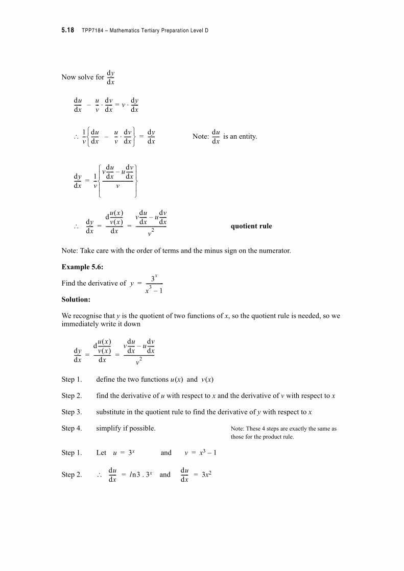
Example 5.6:
Find the derivative of
Solution:
We recognise that y is the quotient of two functions of x, so the quotient rule is needed, so we immediately write it down
Step 1. define the two functions u(x) and v(x)
Step 2. find the derivative of u with respect to x and the derivative of v with respect to x
Step 3. substitute in the quotient rule to find the derivative of y with respect to x
Step 4. simplify if possible. Note: These 4 steps are exactly the same as
those for the product rule.
Step 1. Let u = 3x and v = x3 – 1
Step 2. " = ln3 . 3x and = 3x2
dy
dx------
du
dx------
u
v---
dv
dx------ v
dy
dx------2=2
1
v---
du
dx------
u
v---
dv
dx------2–
3 45 67 8 dy
dx------=
du
dx------
dy
dx------
1
v---
vdu
dx------ u
dv
dx------–
v-------------------------
3 49 95 69 97 8
=
dy
dx------
du x !v x !----------
dx--------------
vdu
dx------ u
dv
dx------–
v2
-------------------------= =
y3
x
x3
1–--------------=
dy
dx------
du x !v x !----------
dx--------------
vdu
dx------ u
dv
dx------–
v2
-------------------------= =
du
dx------
du
dx------
Module 5 – Calculus 5.19
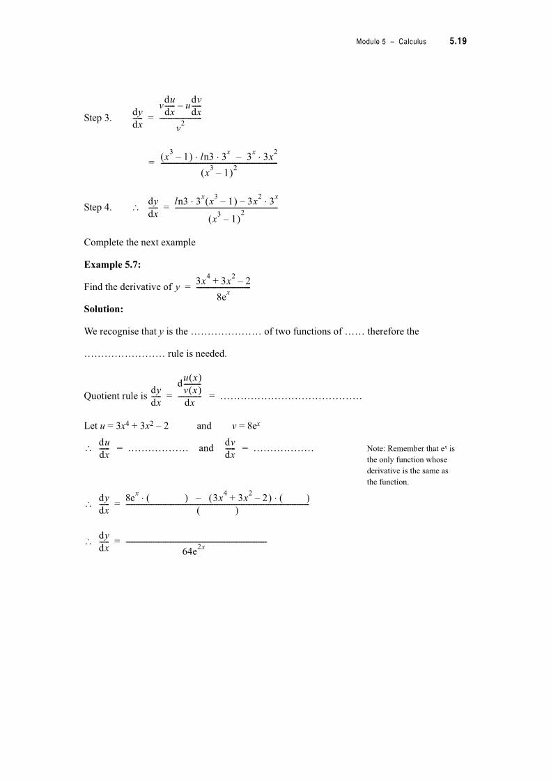
Step 3.
=
Step 4. "
Complete the next example
Example 5.7:
Find the derivative of
Solution:
We recognise that y is the ………………… of two functions of …… therefore the
…………………… rule is needed.
Quotient rule is = ……………………………………
Let u = 3x4 + 3x2 – 2 and v = 8ex
" = ……………… and = ……………… Note: Remember that ex is
the only function whose
derivative is the same as
the function.
"
"
dy
dx------
vdu
dx------ u
dv
dx------–
v2
-------------------------=
x3
1– ! ln3 3x2 3
x3x
22–2
x3
1– !2---------------------------------------------------------------------
dy
dx------
ln3 3x
x3
1– ! 3x2
3x2–2
x3
1– !2
-------------------------------------------------------------=
y3x
43x
22–+
8ex
--------------------------------=
dy
dx------
du x !v x !----------
dx--------------=
du
dx------
dv
dx------
dy
dx------
8ex !2 3x
43x
22–+ ! !2–
!------------------------------------------------------------------------------------------------------------=
dy
dx------
64e2x
-----------------------------------------------------------------------------------=
5.20 TPP7184 – Mathematics Tertiary Preparation Level D
Exercise Set 5.4
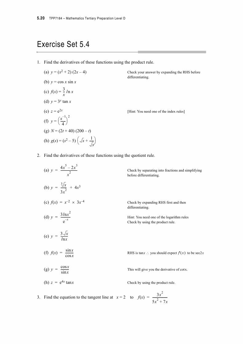
1. Find the derivatives of these functions using the product rule.
(a) y = (x2 + 2) (2x – 4) Check your answer by expanding the RHS before
differentiating.
(b) y = cos x sin x
(c) f(x) = ln x
(d) y = 3x tan x
(e) z = e2x [Hint: You need one of the index rules]
(f) y =
(g) N = (2t + 40) (200 – t)
(h) g(s) = (s2 – 5)
2. Find the derivatives of these functions using the quotient rule.
(a) y = Check by separating into fractions and simplifying
before differentiating.
(b) y = + 4x3
(c) f(x) = x–2 ' 3x–4 Check by expanding RHS first and then
differentiating.
(d) y = Hint: You need one of the logarithm rules
Check by using the product rule.
(e) y =
(f) f(x) = RHS is tanx " you should expect to be sec2x
(g) y = This will give you the derivative of cotx.
(h) z = e4x tanx Check by using the product rule.
3. Find the equation to the tangent line at x = 2 to f(x) =
3
x---
x1–
4-------( )
, -2
s1
s------+( )
, -
4x5
2x3
–
x2
----------------------
x3
3x2
--------
3lnx2
ex–
-------------
3 x
lnx----------
xsin
xcos----------- f' x !
xcos
xsin-----------
3x2
5x2
7x+--------------------
Module 5 – Calculus 5.21
4. (a) Find for the following functions without multiplying out first.
(i) f(x) = (x – 1) (x – 2)
(ii) f(x) = (x – 1) (x – 2) (x – 3) [Hint: Bracket some factors]
(iii) f(x) = (x – 1) (x – 2) (x – 3) (x – 4)
(b) Use the results from (a) to write a general rule for for
f(x) = (x – r1) (x – r2) (x – r3) (x – r4) … (x – rn – 1) (x – rn)
where r1, r2, r3, …, rn are real numbers.
The Chain Rule
So far we have only been dealing with simple relations that are functions of only one variable. In many applications of science, engineering and business we have composite functions and functions of several variables. For example, if a stone is dropped into a pond it sends out circular ripples. The area A, of the outermost ripple depends on the radius r, of the ripple. However, this radius is changing time since the stone was thrown. So the area of the ripple is a function of the radius of the ripple, which is a function of the time elapsed. In function notation we write this as:
A = A(r(t)) Note: Revise composite functions if you are
unsure of this notation.
If a small change in t occurs this will generate a small change in r, which in turn will generate a small change in A. We can see that a small change in t ends up generating a small change in A. When this is the situation the result is
=
By using a similar approach to finding derivatives of simple functions from first principles, and considering the limit of each expression as 1A, 1r and 1t % 0 the result is:
=
In general, if y is a function of z, and z is a function of x, then y is a function of x and we use the Chain Rule to find the derivative of y with respect to x.
f ' x !
f ' x !
1A
1t-------
1A
1r-------
1r
1t------2
dA
dt-------
dA
dr-------
dr
dt-----2
=dy
dx------
dy
dz------
dz
dx------2
5.22 TPP7184 – Mathematics Tertiary Preparation Level D
Example 5.8:
Find the rate of change of the area of a circular ripple with respect to time if you observe that the radius of the outermost ripple is increasing a 2 ms–1. How fast is the ripple spreading when the radius is 3 m?
Solution:
Although we have already established that here we are dealing with a function of a function and hence the chain rule will be needed, the general approach for this type of problem is demonstrated below.
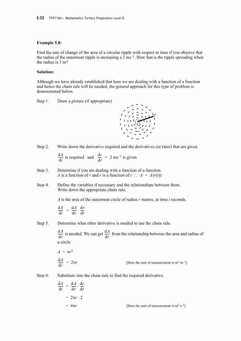
Step 1. Draw a picture (if appropriate)
Step 2. Write down the derivative required and the derivatives (or rates) that are given.
is required and = 2 ms–1 is given
Step 3. Determine if you are dealing with a function of a function.A is a function of r and r is a function of t " A = A(r(t))
Step 4. Define the variables if necessary and the relationships between them.Write down the appropriate chain rule.
A is the area of the outermost circle of radius r metres, at time t seconds.
=
Step 5. Determine what other derivative is needed to use the chain rule.
is needed. We can get from the relationship between the area and radius of
a circle.
A = #r2
= 2#r [Here the unit of measurement is m2 m–1]
Step 6. Substitute into the chain rule to find the required derivative.
=
= 2#r . 2
= 4#r [Here the unit of measurement is m2 s–1]
r
dA
dt-------
dr
dt-----
dA
dt-------
dA
dr-------
dr
dt-----2
dA
dr-------
dA
dr-------
dA
dr-------
dA
dt-------
dA
dr-------
dr
dt-----2
Module 5 – Calculus 5.23
Step 7. Evaluate the derivative for the specified value of interest.
When r = 3 m
= 4# ' 3
= 12# m2s–1
Step 8. Check that the answer looks sensible for the given information and express your answer in a sentence.
12# m2s–1 is about 36 square metres per second which appears reasonable given the rate at which the radius is changing.
Answer: When the radius is 3 m, the area of the outermost ripple is increasing at the rate of 12# m2s–1
Example 5.9:
Find the derivative of y = tan x3
Solution:
Step 1. A diagram is not appropriate here.
Step 2. The required derivative is .
Step 3. We recognise that y is a function of a function comprised of a cubic function inside a tan function "we need the chain rule.
Step 4. To write down the appropriate chain rule, we need to define some variables. Let’s define the variable z.
Let z = x3 " y = tan z i.e. y = y(z(x))
" =
Step 5. We need to find and from the relationship between y and z and the
relationship between z and x.
If y = tan z and if z = x3
= sec2 z = 3x2
= sec2(x3) See Note 1
Notes
1. We don’t want z appearing in our final solution so we have to substitute for z.
dA
dt-------
dy
dx------
dy
dx------
dy
dz------
dz
dx------2
dy
dz------
dz
dx------
dy
dz------
dz
dx------
5.24 TPP7184 – Mathematics Tertiary Preparation Level D
Step 6. Substituting in the chain rule gives
= sec2(x3) . 3x2
= 3x2sec2(x3)
Step 7. No particular value of the derivative is required.
Step 8. This is not an applied problem so there is no need to express your answer in a sentence.
In the following example I have not included all the steps but you should be able to follow the procedure. If you can’t, write out the steps and show extra working where appropriate.Example 5.10:
If y = , find the derivative of y with respect to t when t = 0.5
Solution:
We recognise that y is function of a function comprised of a quadratic function inside an exponential function.
As y is function of a function we need the chain rule to differentiate y.
The general chain rule is
= for y = y(z(t))
Defining the variable z as z(t) = 3t2 , we see that y(z) = ez and thus y = y(z(t))
The particular chain rule required is
=
Finding and
If y = ez and if z = 3t2
= ez = 6t
=
dy
dx------
e3t
2
dy
dt------
dy
dz------
dz
dt-----2
dy
dt------
dy
dz------
dz
dt-----2
dy
dz------
dz
dt-----
dy
dz------
dz
dt-----
e3t
2
Module 5 – Calculus 5.25
Substituting into the chain rule gives
= . 6t
=
Note carefully that you can eliminate some steps by doing the substitution of z “in your head”.
Look at the result for . It is the product of the derivative of the “outside function”
(assuming z had been substituted) and the derivative of the “inside function” (i.e. of z).
So if y = we can get by multiplying the derivative of the outside function
(i.e. ) by the derivative of the inside function (i.e. 6t).
=
We need to find when t = 0.5
= 6 ' 0.5 '
= 6.351
Often when you are using the product rule or the quotient rule you will have to use the chain rule as well. For example, if y = sin x . ln(1 – 3x2), the first thing to notice is that y is the product of the two functions, sin x and ln(1 – 3x2), so the product rule is needed.
Now we notice that ln(1 – 3x2) is a composite function, so when we come to find its derivative to use in the product rule we will have to use the chain rule.
Although this may seem complicated it is quite easy if you follow a procedure such as the one shown below. (Note that the steps are not explicity shown, but if you have any difficulty following the solution you should rewrite it and show each step.)
Example 5.11:
Find the derivative with respect to x of y = sin x . ln(1 – 3x2)
Solution:
y is the product of two functions so the product rule is needed.
General product rule is
= +
dy
dt------ e
3t2
6te3t
2
dy
dt------
e3 t
2 dy
dt------
e3 t
2
dy
dt------ 6te
3 t2
dy
dt------
dy
dt------ e
3 0.5 !2
du v2dx
------------- udv
dx------2 v
du
dx------2
5.26 TPP7184 – Mathematics Tertiary Preparation Level D
Let u = sin x and v = ln(1 – 3x2) {Note that v is function of function so to
find its derivative the chain rule is
needed.}
" = cos x
Let z = (1 – 3x2) " v = ln z i.e. v = v(z(x))
" The chain rule needed is:
=
= –6x and =
=
Substituting into the chain rule gives:
= . (–6x)
= See Note 1
Now substituting in the product rule gives:
= sin x . + ln(1 – 3x2) . cos x
Now we simplify if possible.
Notes
1. You may like to write as .
du
dx------
dv
dx------
dv
dz------
dz
dx------2
dz
dx------
dv
dz------
1
z---
1
1 3x2
–-----------------
dv
dx------
1
1 3x2
–-----------------
6x–
1 3x2
–-----------------
6x–
1 3x2–-----------------
6x
3x2 1–-----------------
du v2dx
-------------6x–
1 3x2
–-----------------
( )* +, -

Module 5 – Calculus 5.27
Exercise Set 5.5
Make sure you do a selection of problems from all questions in this Exercise Set.1. Find the derivatives of the following.
(a) y = ln(2x3 + x)
(b) y = 2e4t + 8t2
(c) y = sin 4x – + {Make sure you do this one}
(d) y = cot2 x {Make sure you do this one too}
(e) y =
2. Find the derivatives with respect to x of the following.
(a) y = ex cos 2x
(b) y = ; also find when x = 3
(c) y = x3esin x
(d) y = ; also find when x = 2
(e) y = ; also find when x =
3.
(a) If = 2 + 3cos x and = 2sin x ,
show that = cosec x +
(b) If = lnx and = , find
(c) If = 4e2t and = e–2t , find when t = 0.25
1
4---x
2cos
x
2---tan
1
2x2
1– !3
------------------------
ln x2
4– !
3x3
2x 4+–-----------------------------
dy
dx------
x4
x4
tan-------------
dy
dx------
x3
cos ex
3sin2
dy
dx------
1
2---
dv
dt------
dv
dx------
dx
dt------
3
2--- xcot
dz
dt-----
dz
dx------
1
x---
dx
dt------
dp
dz------
dp
dt------
dz
dt-----

5.28 TPP7184 – Mathematics Tertiary Preparation Level D
4.(a) The population N, of a bacterial colony is given by N = Cekt where t is the time in
seconds and C and k are constants. Find the rate of increase of the population after 6 seconds.
(b) A radioactive substance decays according to the relationship x = where x0 is
the initial amount in kilograms and t is the time in years. Find the rate of decay of an initial amount of 250 kg after 10 years.
(c) The temperature T, of a body (in centigrade) which is allowed to cool in a room with air temperature of Ta at any time t (in seconds) is given by
T – Ta = (To – Ta) e–0.05596t
where To is the initial temperature of the body. Find the rate of cooling of the body if
initially it was 90:C and the air temperature is 20:C.
5.(a) If a metal disc with radius r cm retains its shape as it expands when heated, how fast is
the radius increasing when the area is increasing at a rate of 0.4 cm2s–1?
(b) If a metal square with sides of length l cm retains its shape as it expands when heated, how fast is the length of a side increasing when the area is increasing at a rate of 0.5 cm2s–1?
6.(a) Let V be the volume and S the total surface area of a solid right circular cylinder that is
7 metres high and has a radius r metres. Find when r = 6 m.
(b) A round balloon is being inflated with helium at the rate of 12 cm3s–1. How fast is the
radius of the balloon expanding when the volume is cm3?
(c) Water is flowing into a conical tank at the rate of 3 m3h–1. The tank has a radius of 4 m at the top and a depth of 7 m. How fast is the water rising when the water level is 2 m?
x0e–
1
2--- t
dV
dS-------
9#2
------
Module 5 – Calculus 5.29
Stationary Points
So far we have been using derivatives to find the rate of change of a function y, for any value
of x, i.e. . We have also seen that we can evaluate for a specific value of x to get
the instantaneous rate of change at the value of interest.
Often we want to determine when the rate of change is zero, i.e. when the gradient is neither increasing nor decreasing because this gives the maximum and minimum values of a function,
i.e. it gives us a mechanism to optimise f(x). Points where are zero are called stationary
points or critical points. A stationary point can be a turning point, i.e. a maximum or a minimum or a point of inflection.
There are two different methods for determining if a stationary point is a maximum or minimum. The first method involves examining the first derivative just before and just after the stationary point. (You should be familiar with this method from Unit 11083 or its equivalent.) The second method involves examining the second derivative at the stationary point.
Let’s start by using the first method.
Example 5.12:
A population p, grows according to the function
p(t) = 1000 + where t is time in hours
Determine when the population is maximised.
Solution:
The maximum will occur when the rate of change of population with respect to time is zero.
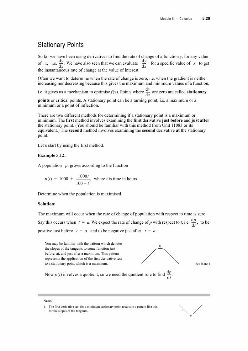
Say this occurs when t = a. We expect the rate of change of p with respect to t, i.e. , to be
positive just before t = a and to be negative just after t = a.
See Note 1
Now p(t) involves a quotient, so we need the quotient rule to find .
Notes
1.
dy
dx------
dy
dx------
dy
dx------
1000t
100 t2
+-------------------
dp
dt------
You may be familiar with the pattern which denotes
the slopes of the tangents to some function just
before, at, and just after a maximum. This pattern
represents the application of the first derivative test
to a stationary point which is a maximum.
0
+ –
The first derivative test for a minimum stationary point results in a pattern like this
for the slopes of the tangents.0
+ –
dp
dt------

5.30 TPP7184 – Mathematics Tertiary Preparation Level D
Once we have we can find out for what values of t it equals zero. These values of t
give the stationary points which then need to be identified.
p(t) = 1000 + = 1000 +
= + = 0 +
Let u = 1000t and v = 100 + t2
" = 1000 " = 2t
" = 0 +
=
=
Now we know stationary points occur when = 0
i.e. when = 0
This equation will be true when the numerator of the LHS equals zero.
i.e. 100000 – 1000t2 = 0
" t2 = 100
" t = +10 or –10
i.e. stationary points occur when t = 10 hours and t = –10 hours.
Now t = –10 hours has no meaning in this problem so we can ignore it.
We now have to determine what sort of stationary point occurs at t = 10.
dp
dt------
1000t
100 t2
+-------------------
u t !v t !---------
dp
dt------
d1000
dt---------------
du
v---
dt------
vdu
dt------ u
dv
dt------–
v2
-------------------------
du
dt------
dv
dt------
dp
dt------
100 t2
+ ! 1000 1000t 2t2–2
100 t2
+ !2
-------------------------------------------------------------------------
100000 1000t2
2000t2
–+
100 t2
+ !2
------------------------------------------------------------------
100000 1000t2
–
100 t2
+ !2
----------------------------------------
dp
dt------
100000 1000t2
–
100 t2
+ !2
----------------------------------------
Module 5 – Calculus 5.31
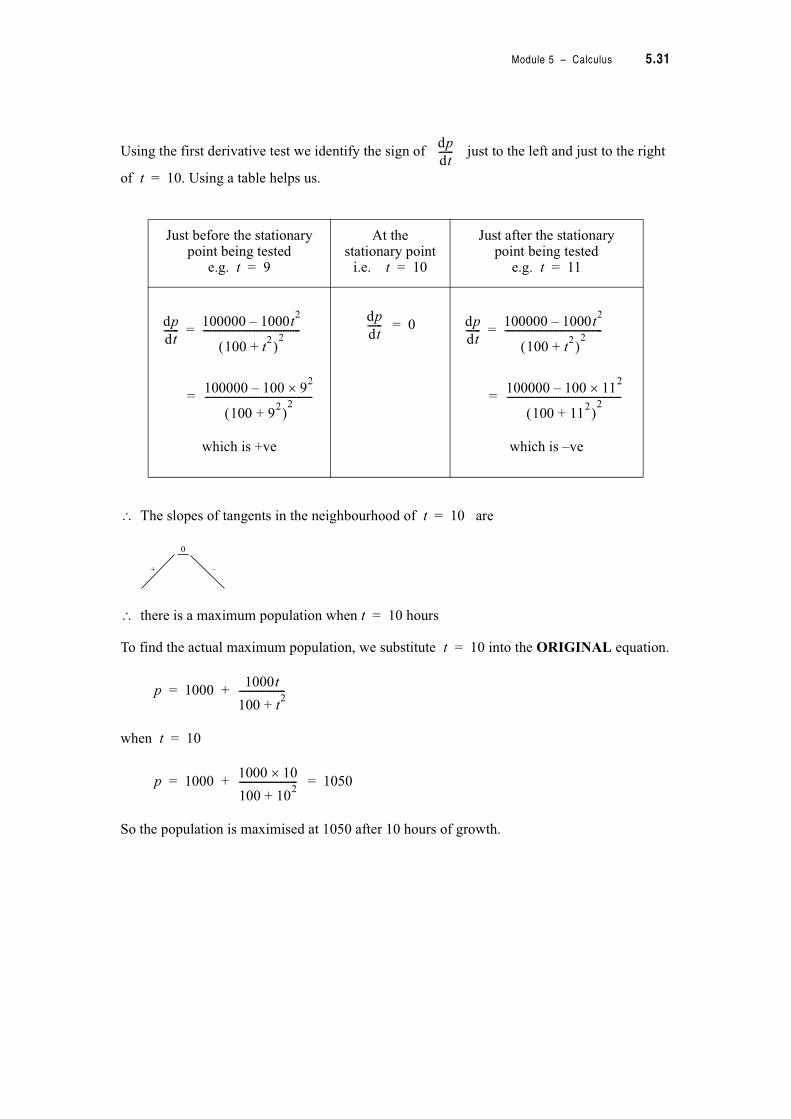
Using the first derivative test we identify the sign of just to the left and just to the right
of t = 10. Using a table helps us.
The slopes of tangents in the neighbourhood of t = 10 are
there is a maximum population when t = 10 hours
To find the actual maximum population, we substitute t = 10 into the ORIGINAL equation.
p = 1000 +
when t = 10
p = 1000 + = 1050
So the population is maximised at 1050 after 10 hours of growth.
Just before the stationary point being tested
e.g. t = 9
At the stationary point
i.e. t = 10
Just after the stationary point being tested
e.g. t = 11
=
which is +ve
= 0
=
which is –ve
dp
dt------
dp
dt------
100000 1000t2
–
100 t2
+! "2
----------------------------------------=
100000 100 92#–
100 92
+! "2
--------------------------------------------
dp
dt------ dp
dt------
100000 1000t2
–
100 t2
+! "2
----------------------------------------=
100000 100 112#–
100 112
+! "2
-----------------------------------------------
0
+ –
1000t
100 t2
+-------------------
1000 10#
100 102
+------------------------
5.32 TPP7184 – Mathematics Tertiary Preparation Level D
Second Derivatives
The second derivative of a function is the function which gives the slope of the gradient function, e.g. it tells us how fast or slow the rate of growth of a population is or the rate of decrease of the unemployment rate, etc.
You are already familiar with second derivatives through the notions of displacement velocity and acceleration. Recall that velocity is the derivative of displacement with respect to time,
i.e. v = or v = and that acceleration is the derivative of velocity with respect to
time,
i.e. a = or a =
a = =
We usually write this as
a = or a =
and read it as ‘acceleration is the second derivative of displacement with respect to time.’ In ‘short-hand’ we say ‘acceleration is dee squared s, dee t squared,’ or ‘acceleration is s double dash t.’
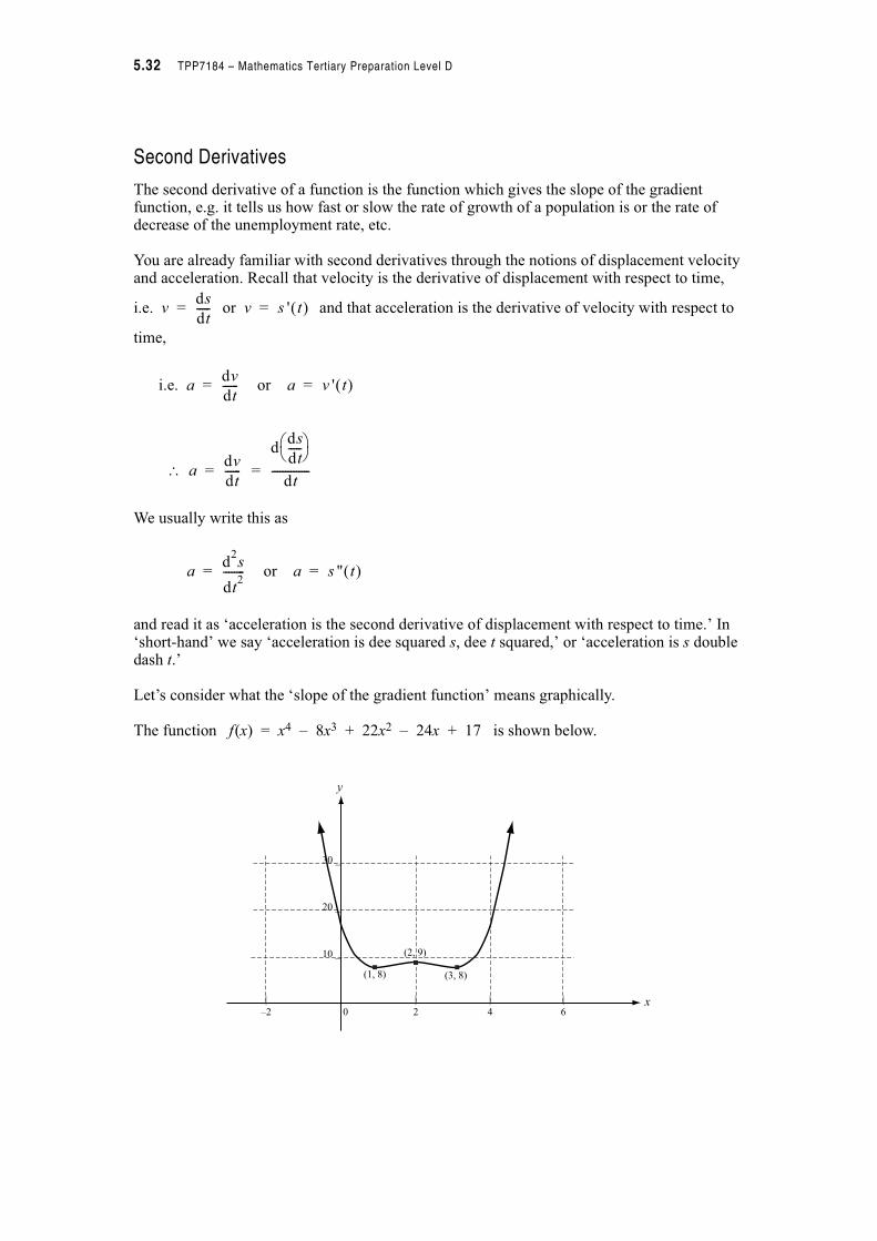
Let’s consider what the ‘slope of the gradient function’ means graphically.
The function f(x) = x4 – 8x3 + 22x2 – 24x + 17 is shown below.
ds
dt----- s ' t! "
dv
dt------ v ' t! "
dv
dt------
dds
dt-----$ %& '
dt--------------
d2s
dt2
-------- s '' t! "
| | | |
–2 0 2 4 6
30 _
20 _
10 _ (2, 9)
(1, 8) (3, 8)
x
y

Module 5 – Calculus 5.33
This function is a quartic, i.e. a polynomial with degree 4 so it is continuous and differentiable for all x values. We can see that: See Note 1
• for x < 1, f(x) is decreasing• for x = 1, f(x) is stationary• for 1 < x < 2, f(x) is increasing• for x = 2, f(x) is stationary• for 2 < x < 3, f(x) is decreasing• for x = 3, f(x) is stationary• for x > 3, f(x) is increasing
We would expect the slope of the tangents to f(x) to have this pattern.
However the magnitudes of the slopes of the tangents are not constant in the various sections of the graph.
Draw the graph of f(x) = x4 – 8x3 + 22x2 – 24x + 17 for 0 < x ( 4 on your computer.
Make sure you do this activity as many important concepts are developed through it.Now we are going to examine various sections of the graph and see what the first and second derivatives tell us about f(x).
Notes
1. As expected f(x) has three turning points.
+
–
–
+0
0 0
5.34 TPP7184 – Mathematics Tertiary Preparation Level D
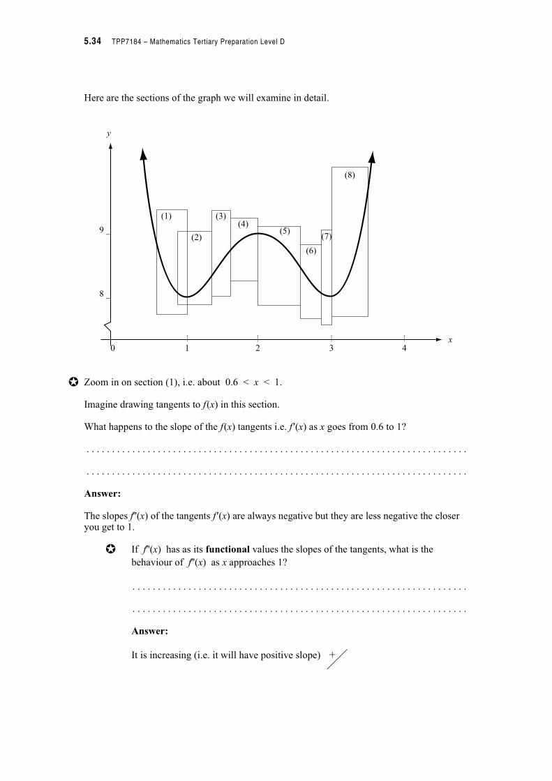
Here are the sections of the graph we will examine in detail.
Zoom in on section (1), i.e. about 0.6 < x < 1.
Imagine drawing tangents to f(x) in this section.
What happens to the slope of the f(x) tangents i.e. f'(x) as x goes from 0.6 to 1?
. . . . . . . . . . . . . . . . . . . . . . . . . . . . . . . . . . . . . . . . . . . . . . . . . . . . . . . . . . . . . . . . . . . . . . . . . . .
. . . . . . . . . . . . . . . . . . . . . . . . . . . . . . . . . . . . . . . . . . . . . . . . . . . . . . . . . . . . . . . . . . . . . . . . . . .
Answer:
The slopes f''(x) of the tangents f'(x) are always negative but they are less negative the closer you get to 1.
If f''(x) has as its functional values the slopes of the tangents, what is the
behaviour of f''(x) as x approaches 1?
. . . . . . . . . . . . . . . . . . . . . . . . . . . . . . . . . . . . . . . . . . . . . . . . . . . . . . . . . . . . . . . . . .
. . . . . . . . . . . . . . . . . . . . . . . . . . . . . . . . . . . . . . . . . . . . . . . . . . . . . . . . . . . . . . . . . .
Answer:
It is increasing (i.e. it will have positive slope)
| | | |
0 1 2 3 4
9 _
8 _
x
y
(1)
(2)
(3)(4)
(5)
(6)
(7)
(8)
+
Module 5 – Calculus 5.35
Does f(x) lie above all the tangents you can draw for x < 1 (i.e. is f(x) bigger
than for any value less than 1)?
. . . . . . . . . . . . . . . . . . . . . . . . . . . . . . . . . . . . . . . . . . . . . . . . . . . . . . . . . . . . . . . . . .
. . . . . . . . . . . . . . . . . . . . . . . . . . . . . . . . . . . . . . . . . . . . . . . . . . . . . . . . . . . . . . . . . .
Answer:
Yes f(x) ) for any x, so we say f(x) is concave up for x < 1.
Zoom in on section (2), i.e. about 0.9 < x < 1.3
What happens to the slope of the tangents as x goes from 0.9 to 1.3?
. . . . . . . . . . . . . . . . . . . . . . . . . . . . . . . . . . . . . . . . . . . . . . . . . . . . . . . . . . . . . . . . . . . . . . . . . . .
. . . . . . . . . . . . . . . . . . . . . . . . . . . . . . . . . . . . . . . . . . . . . . . . . . . . . . . . . . . . . . . . . . . . . . . . . . .
Answer:
Before x = 1, the tangents have negative slopes but they are less negative the closer you get to 1. At exactly x = 1, the tangent is parallel with the x-axis, thus it has zero slope. After x = 1, the tangent slopes change sign and have positive slopes and the further you go from x = 1 the greater the slope.
If has as its functional values the slopes of the tangents what is the
behaviour of f''(x) near x = 1?
. . . . . . . . . . . . . . . . . . . . . . . . . . . . . . . . . . . . . . . . . . . . . . . . . . . . . . . . . . . . . . . . . .
. . . . . . . . . . . . . . . . . . . . . . . . . . . . . . . . . . . . . . . . . . . . . . . . . . . . . . . . . . . . . . . . . .
Answer:
It is increasing (i.e. it will have positive slope)
Does f(x) lie above all the tangents you can draw for x < 1.3? . . . . . . . . . . . . .
Is f(x) still concave up? . . . . . . . . . . . . . . . . . . . . . . . . . . . . . . . . . . . . . . . . . . . . . .
Answer:
Yes f(x) is concave up for any x value up to about x = 1.3.
f ' x! "
f ' x! "
f ' x! "
+

5.36 TPP7184 – Mathematics Tertiary Preparation Level D
Zoom in on section (3), i.e. about 1.3 < x < 1.6
What happens to the slopes of the tangents as x goes from 1.3 to 1.6?
. . . . . . . . . . . . . . . . . . . . . . . . . . . . . . . . . . . . . . . . . . . . . . . . . . . . . . . . . . . . . . . . . . . . . . . . . . .
. . . . . . . . . . . . . . . . . . . . . . . . . . . . . . . . . . . . . . . . . . . . . . . . . . . . . . . . . . . . . . . . . . . . . . . . . . .
Answer:
Up to about x = 1.4 the tangents have increasing positive slope but after about x = 1.4, although the slopes remain positive the tangents start to flatten out, i.e. their slopes decrease the further away from x = 1.4 you go.
What does this mean about ?
………………………………………………………………………………
………………………………………………………………………………
Answer:
The derivative function has a maximum at about x = 1.4.
Does f(x) lie above all the tangents you can draw for 1.3 < x < 1.6? What do
you think this means about the concavity of f(x) in this section?
. . . . . . . . . . . . . . . . . . . . . . . . . . . . . . . . . . . . . . . . . . . . . . . . . . . . . . . . . . . . . . . . . .
. . . . . . . . . . . . . . . . . . . . . . . . . . . . . . . . . . . . . . . . . . . . . . . . . . . . . . . . . . . . . . . . . .
Answer:
f(x) lies above the tangents (i.e.f(x) > ) up to about x = 1.4 so f(x) is
concave up to x * 1.4. But f(x) lies below the tangents for x between about 1.4 and
1.6, i.e. f(x) < for x between about 1.4 and 1.6. We say f(x) is concave
down for x between about 1.4 and 1.6.
Before we examine the remaining sections of f(x), let’s summarise what we’ve found about f(x) for 0.6 < x < 1.6. (As the function is well behaved i.e. we can consider –+ < x < 1.6)
f ' x! "
f ' x! "
f ' x! "
f ' x! "
Module 5 – Calculus 5.37
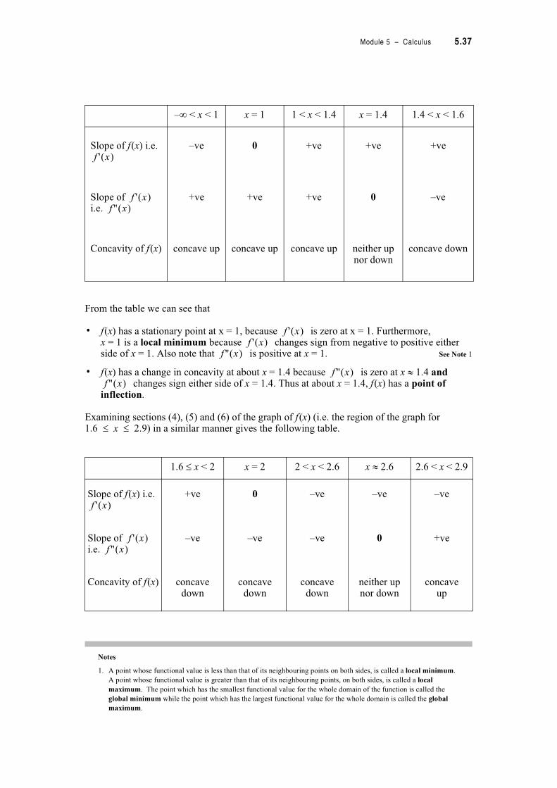
From the table we can see that
• f(x) has a stationary point at x = 1, because is zero at x = 1. Furthermore, x = 1 is a local minimum because changes sign from negative to positive either side of x = 1. Also note that is positive at x = 1. See Note 1
• f(x) has a change in concavity at about x = 1.4 because is zero at x * 1.4 and changes sign either side of x = 1.4. Thus at about x = 1.4, f(x) has a point of
inflection.
Examining sections (4), (5) and (6) of the graph of f(x) (i.e. the region of the graph for 1.6 ( x ( 2.9) in a similar manner gives the following table.
–+ < x < 1 x = 1 1 < x < 1.4 x = 1.4 1.4 < x < 1.6
Slope of f(x) i.e. –ve 0 +ve +ve +ve
Slope of i.e.
+ve +ve +ve 0 –ve
Concavity of f(x) concave up concave up concave up neither up nor down
concave down
Notes
1. A point whose functional value is less than that of its neighbouring points on both sides, is called a local minimum.
A point whose functional value is greater than that of its neighbouring points, on both sides, is called a local
maximum. The point which has the smallest functional value for the whole domain of the function is called the
global minimum while the point which has the largest functional value for the whole domain is called the global
maximum.
1.6 ( x < 2 x = 2 2 < x < 2.6 x * 2.6 2.6 < x < 2.9
Slope of f(x) i.e. +ve 0 –ve –ve –ve
Slope of i.e.
–ve –ve –ve 0 +ve
Concavity of f(x) concavedown
concavedown
concavedown
neither upnor down
concaveup
f ' x! "
f ' x! "f '' x! "
f ' x! "f ' x! "
f '' x! "
f '' x! "f '' x! "
f ' x! "
f ' x! "f '' x! "
5.38 TPP7184 – Mathematics Tertiary Preparation Level D
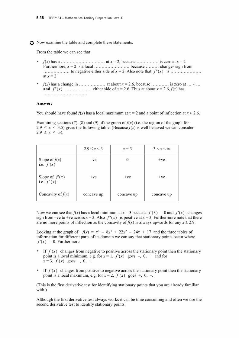
Now examine the table and complete these statements.
From the table we can see that
• f(x) has a ………………………… at x = 2, because …………… is zero at x = 2 Furthermore, x = 2 is a local …………………… because ……… changes sign from ……………… to negative either side of x = 2. Also note that is ………………… at x = 2
• f(x) has a change in ……………… at about x = 2.6, because ………… is zero at … * … and ……………… either side of x = 2.6. Thus at about x = 2.6, f(x) has …………………………
Answer:
You should have found f(x) has a local maximum at x = 2 and a point of inflection at x * 2.6.
Examining sections (7), (8) and (9) of the graph of f(x) (i.e. the region of the graph for 2.9 ( x < 3.5) gives the following table. (Because f(x) is well behaved we can consider2.9 ( x < +).
Now we can see that f(x) has a local minimum at x = 3 because = 0 and changes sign from –ve to +ve across x = 3. Also is positive at x = 3. Furthermore note that there are no more points of inflection as the concavity of f(x) is always upwards for any x , 2.9.
Looking at the graph of f(x) = x4 – 8x3 + 22x2 – 24x + 17 and the three tables of information for different parts of its domain we can say that stationary points occur where
= 0. Furthermore
• If changes from negative to positive across the stationary point then the stationary point is a local minimum, e.g. for x = 1, goes –, 0, + and for x = 3, goes –, 0, +.
• If changes from positive to negative across the stationary point then the stationary point is a local maximum, e.g. for x = 2, goes +, 0, –.
(This is the first derivative test for identifying stationary points that you are already familiar with.)
Although the first derivative test always works it can be time consuming and often we use the second derivative test to identify stationary points.
2.9 ( x < 3 x = 3 3 < x < +
Slope of f(x)i.e.
–ve 0 +ve
Slope of i.e.
+ve +ve +ve
Concavity of f(x) concave up concave up concave up
f '' x! "
f '' x! "
f ' x! "
f ' x! "f '' x! "
f ' 3! " f ' x! "f '' x! "
f ' x! "
f ' x! "f ' x! "
f ' x! "
f ' x! "f ' x! "
Module 5 – Calculus 5.39
Identifying Stationary Points Using the Second Derivative Test
Looking again at the graph of f(x) = x4 – 8x3 + 22x2 – 24x + 17 and the three tables of information we can also identify the stationary points by considering the sign of the second derivative at each point of interest.
• If a function has a stationary point at say x = a and if is positive - a is a local minimum.
e.g. for x = 1, is +ve
for x = 3, is +ve
• If a function has a stationary point at say x = a and if is negative - a is a local maximum.
e.g. for x = 2, is –ve
Note: If then no conclusion can be made about the type of stationary point a is. It could be a maximum, a minimum or a point of inflection. You have to go back and examine each side of a to decide if a is a maximum or a minimum; while a change in concavity (i.e. if changes sign across x = a) shows a point of inflection at x = a.
Points of inflection occur where = 0 and there is a change in concavity across the point of interest.
Note: All smooth continuous functions (such as polynomials) have a point of inflection between every maximum and minimum.
Example 5.13:
Find the local maxima and minima and any points of inflection forf(x) = 2x3 – 21x2 + 36x – 8
Solution:
Step 1. Find stationary points
Stationary points occur where = 0
= 6x2 – 42x + 36
Setting to zero yields
6x2 – 42x + 36 = 0
x2 – 7x + 6 = 0
(x – 6) (x – 1) = 0
x = 6 and x = 1 are stationary points.
f '' a! "
f '' 1! "
f '' 3! "
f '' a! "
f '' 2! "
f '' a! " 0=
f ' x! "f '' x! "
f '' x! "
f ' x! "
f ' x! "
f ' x! "
5.40 TPP7184 – Mathematics Tertiary Preparation Level D
Step 2. Identify stationary points
(I’ll choose to use the second derivative test.)
= 12x – 42
When x = 6, = 12 # 6 – 42 i.e. +ve - minium at x = 6
When x = 1, = 12 # 1 – 42 i.e. –ve - maximum at x = 1
Step 3. Find potential points of inflection
Points of inflection may occur when = 0
i.e. 12x – 42 = 0
x =
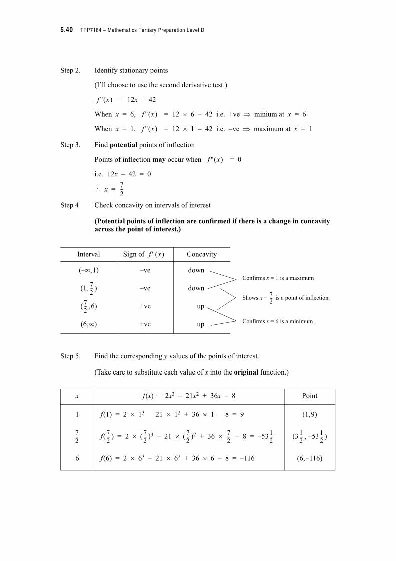
Step 4 Check concavity on intervals of interest
(Potential points of inflection are confirmed if there is a change in concavity across the point of interest.)
Step 5. Find the corresponding y values of the points of interest.
(Take care to substitute each value of x into the original function.)
x f(x) = 2x3 – 21x2 + 36x – 8 Point
1 f(1) = 2 # 13 – 21 # 12 + 36 # 1 – 8 = 9 (1,9)
f( ) = 2 # ( )3 – 21 # ( )2 + 36 # – 8 = –53 (3 , –53 )
6 f(6) = 2 # 63 – 21 # 62 + 36 # 6 – 8 = –116 (6,–116)
f '' x! "
f '' x! "
f '' x! "
f '' x! "
7
2---
Interval Sign of Concavity
(–+,1) –ve down
(1, ) –ve down
( ,6) +ve up
(6,+) +ve up
f '' x! "
7
2---
7
2---
Confirms x = 1 is a maximum
Confirms x = 6 is a minimum
Shows x = is a point of inflection.7
2---
7
2---
7
2---
7
2---
7
2---
7
2---
1
2---
1
2---
1
2---
Module 5 – Calculus 5.41
Step 6. Write a conclusion.
A local minimum occurs at (6,–116), a local maximum occurs at (1,9) and a point
of inflection occurs at (3 , –53 ).
Note: In this problem we have found the local (or relative) maxima and minima off(x) = 2x3 – 21x2 + 36x – 8. Because the domain of f(x) is not limited in any way, we assume –+ < x < +. So the global maximum for f(x) will occur either at one of the local maxima or when x = +, and the global minimum for f(x) will occur either at one of the local minima or when x = –+.
Explain why in this example the global maximum will occur at x = + and the global minimum will occur at x = –+.
. . . . . . . . . . . . . . . . . . . . . . . . . . . . . . . . . . . . . . . . . . . . . . . . . . . . . . . . . . . . . . . . . . . . . . . . . . .
. . . . . . . . . . . . . . . . . . . . . . . . . . . . . . . . . . . . . . . . . . . . . . . . . . . . . . . . . . . . . . . . . . . . . . . . . . .
. . . . . . . . . . . . . . . . . . . . . . . . . . . . . . . . . . . . . . . . . . . . . . . . . . . . . . . . . . . . . . . . . . . . . . . . . . .
Answer:
The dominant term in f(x) = 2x3 – 21x2 + 36x – 8 is the x cubed term so we need to see what happens to this term as x . + and x . –+.
As x . +, 2x3 . + - global maximum at x = +
As x . –+, 2x3 . –+ - global minimum at x = –+
When a domain is restricted we have to be careful to check the local maxima and local minima and the end points of the domain when finding the global maximum or global minimum. This is especially important in applied maximum or minimum problems which we will discuss shortly.
1
2---
1
2---
5.42 TPP7184 – Mathematics Tertiary Preparation Level D
Exercise Set 5.6
1. Find the points of inflection, local maxima and minima and where the given curves are concave up and concave down.
(a) y = x2 + 3x – 8
(b) f(x) = x3 + 6x2 – 15x + 8
(c) f(x) = x4 – 4x3 + 6
(d) f(x) = x +
2. Using a standard test to measure performance, a psychologist finds that an average person’s score, P(t) on a particular test is given by P(t) = 12t2 – t3 for0 ( t ( 12 where t is the number of weeks of study for the test.
After how many weeks of study would the psychologist conclude that the learning has started to decrease?
3. An object is propelled vertically upward with an initial velocity of 39.2 metres per second. The distance s (in metres) of the object from the ground after t seconds is given bys = –4.9t2 + 39.2t.
(i) What is the velocity of the object at any time t?
(ii) When will the object reach its highest point?
(iii) What is the maximum height?
(iv) What is the acceleration of the object at any time t?
(v) How long is the object in the air?
(vi) What is the velocity of the object upon impact?
1
x---
Module 5 – Calculus 5.43
Now you are familiar with first and second derivatives and their use for finding local maximum and minimum points and points of inflection, we can use differentiation to help draw graphs. A useful procedure for sketching the graph of f(x) follows.
Curve Sketching
Step 1. Find where f(x) cuts the y axis
i.e. find f(x) when x = 0
Step 2. Find where f(x) cuts the x axis
i.e. find x when f(x) = 0
Step 3. Identify vertical asymptotes
Step 4. Find stationary points
i.e. find x when = 0
Step 5. Identify stationary points
– use either the second derivative test or the first derivative test
Step 6. Find potential points of inflection
i.e. find x when = 0
Step 7. Check concavity on intervals of interest and identify any points of inflection
Step 8. Find f(x) values for each stationary point and point of inflection
Step 9. Look at the long term behaviour of f(x)
i.e. examine f(x) as x . + and as x . –+
Step 10. Draw graph
Now let’s use this procedure in an example.
f ' x! "
f '' x! "
5.44 TPP7184 – Mathematics Tertiary Preparation Level D
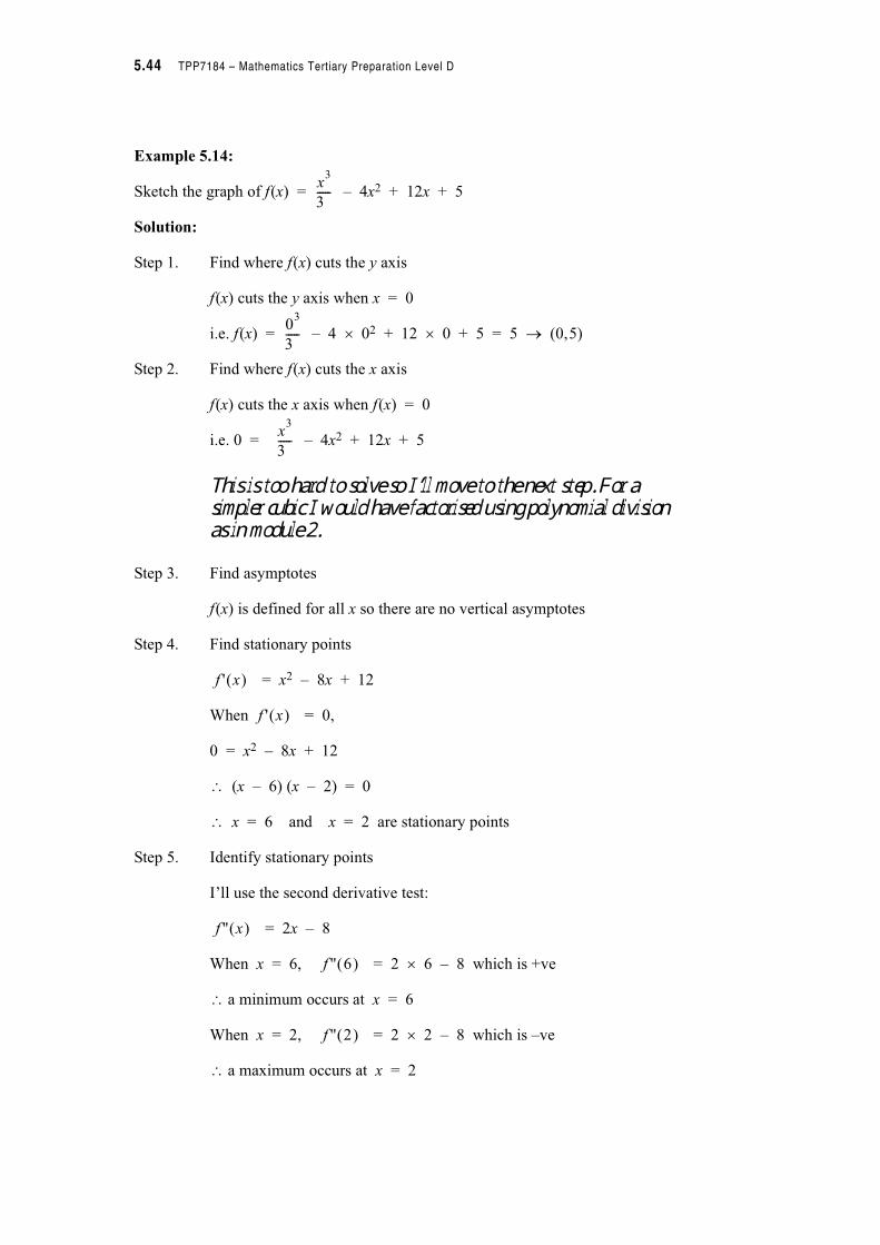
Example 5.14:
Sketch the graph of f(x) = – 4x2 + 12x + 5
Solution:
Step 1. Find where f(x) cuts the y axis
f(x) cuts the y axis when x = 0
i.e. f(x) = – 4 # 02 + 12 # 0 + 5 = 5 . (0,5)
Step 2. Find where f(x) cuts the x axis
f(x) cuts the x axis when f(x) = 0
i.e. 0 = – 4x2 + 12x + 5
This is too hard to solve so I’ll move to the next step. For a simpler cubic I would have factorised using polynomial division as in module 2.Step 3. Find asymptotes
f(x) is defined for all x so there are no vertical asymptotes
Step 4. Find stationary points
= x2 – 8x + 12
When = 0,
0 = x2 – 8x + 12
(x – 6) (x – 2) = 0
x = 6 and x = 2 are stationary points
Step 5. Identify stationary points
I’ll use the second derivative test:
= 2x – 8
When x = 6, = 2 ! 6 – 8 which is +ve
a minimum occurs at x = 6
When x = 2, = 2 ! 2 – 8 which is –ve
a maximum occurs at x = 2
x3
3-----
03
3-----
x3
3-----
f ' x" #
f ' x" #
f '' x" #
f '' 6" #
f '' 2" #

Module 5 – Calculus 5.45
Step 6. Find potential points of inflection
= 2x – 8
When = 0
0 = 2x – 8
x = 4
Step 7. Check concavity on intervals of interest
Step 8. Find f(x) values for each point of interest
Step 9. Look at the long term behaviour of f(x)
f(x) = – 4x2 + 12x + 5
as x $ ×, f(x) $ ×
as x $ –×, f(x) $ –×
x f(x) = – 4x2 + 12x + 5 Point
2 f(2) = – 4 ! 22 + 12 ! 2 + 5 = (2, )
4 f(4) = – 4 ! 42 + 12 ! 4 + 5 = (4, )
6 f(6) = – 4 ! 62 + 12 ! 6 + 5 = 5 (6,5)
f '' x" #
f '' x" #
Interval Sign of Concavity
(–%,2) –ve down
(2,4) –ve down
(4,6) +ve up
(6,%) +ve up
f '' x" #
Confirms maximum at x = 2
Confirms minimum at x = 6
& Point of inflection at x = 4
x3
3-----
23
3----- 15
2
3--- 15
2
3---
43
3----- 10
1
3--- 10
1
3---
63
3-----
x3
3-----
5.46 TPP7184 – Mathematics Tertiary Preparation Level D
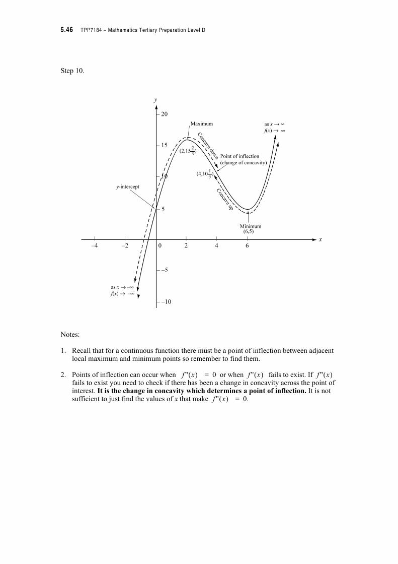
Step 10.
Notes:
1. Recall that for a continuous function there must be a point of inflection between adjacent local maximum and minimum points so remember to find them.
2. Points of inflection can occur when = 0 or when fails to exist. If fails to exist you need to check if there has been a change in concavity across the point of interest. It is the change in concavity which determines a point of inflection. It is not sufficient to just find the values of x that make = 0.
| | | | |
–4 –2 0 2 4 6
– 15
– 10
– 5
– –5
– –10
– 20
Maximum
Point of inflection
(change of concavity)
y-intercept
Minimum
as x→ –∞
f(x) → –∞
as x→ ∞
f(x) → ∞
(2,15 )2
3
(4,10 )1
3
(6,5)
Concave up
Concave dow
n
x
y
f '' x" # f '' x" # f '' x" #
f '' x" #
Module 5 – Calculus 5.47
Exercise Set 5.7
1. Use differentiation to help draw (by hand) each of these functions.
(a) f(x) = 2x3 – 9x2 + 12x – 5
(b) f(x) = x3 – 3x
(c) f(x) = x3 + 3x2 + 3x
2. Use calculus to help draw by hand the graph of
(a) f(x) = xe–x
(b) f(x) = x + sin x for 0 ' x ' 10
3.(a) Find the global maximum and minimum of f(x) = x3 – 9x2 – 48x
for –5 ' x ' 12
(b) Consider f(x) = x – lnx for 0.1 ' x ' 2. Find the global maximum and global minimum
[Check your results by drawing f(x) for (a) and (b) above on the computer]
5.48 TPP7184 – Mathematics Tertiary Preparation Level D
Maximum/Minimum Problems
These problems are very important applications of differentiation. Often the problem is not presented in mathematical terms but rather as words in a sentence, and you have to interpret or identify from the given information what is to be optimised and any constraints that exist on the system. See Note 1
In building the mathematical model (equation) that describes the system we must use many skills. Then follows the solution of the mathematical problem and finally the interpretation of the results in the ‘language’ of the original problem. (Generally in modelling one further step is required, i.e. the validation of your model by comparing its theoretical output with some observed data – you will not be required to perform this final step in this course.) A useful procedure to follow is
Build
Step 1. Draw a sketch if possible.
Step 2. Label all parts. Define all variables.
Step 3. Identify the variable to be optimised, Z, (say)
Step 4. Find an equation expressing Z in terms of other variables (the principal equation).
Step 5. Find any other equations relating variables (the auxiliary equations).
Step 6. Determine any constraints on the system.
Solve
Step 7. Use auxiliary equations to reduce the principal equation to one containing Z and only one independent variable.
Step 8. Determine the interval within which the independent variable must lie.
Step 9. Find the global maximum (minimum) in this interval, Z* by evaluating Z at the stationary points and the end points of the interval.
Interpret
Step 10. From the auxiliary equations find the corresponding values of the other variables.
Step 11. Make a conclusion in the language of the original problem.
Let’s apply this procedure to an example. Note that not all the steps are applicable for every problem.
Notes
1. This is similar to what you did in linear programming problems in Module 2.
Module 5 – Calculus 5.49
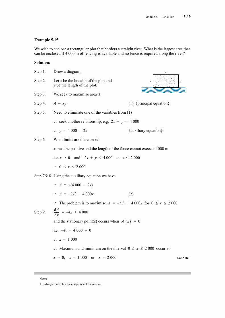
Example 5.15
We wish to enclose a rectangular plot that borders a straight river. What is the largest area that can be enclosed if 4 000 m of fencing is available and no fence is required along the river?
Solution:
Step 1. Draw a diagram.
Step 2. Let x be the breadth of the plot andy be the length of the plot.
Step 3. We seek to maximise area A.
Step 4. A = xy (1) {principal equation}
Step 5. Need to eliminate one of the variables from (1)
seek another relationship, e.g. 2x + y = 4 000
y = 4 000 – 2x {auxiliary equation}
Step 6. What limits are there on x?
x must be positive and the length of the fence cannot exceed 4 000 m
i.e. x ( 0 and 2x + y ' 4 000 x ' 2 000
0 ' x ' 2 000
Step 7& 8. Using the auxiliary equation we have
A = x(4 000 – 2x)
A = –2x2 + 4 000x (2)
The problem is to maximise A = –2x2 + 4 000x for 0 ' x ' 2 000
Step 9. = –4x + 4 000
and the stationary point(s) occurs when = 0
i.e. –4x + 4 000 = 0
x = 1 000
Maximum and minimum on the interval 0 ' x ' 2 000 occur at
x = 0, x = 1 000 or x = 2 000 See Note 1
Notes
1. Always remember the end points of the interval.
x x
y
A
dA
dx-------
A ' x" #
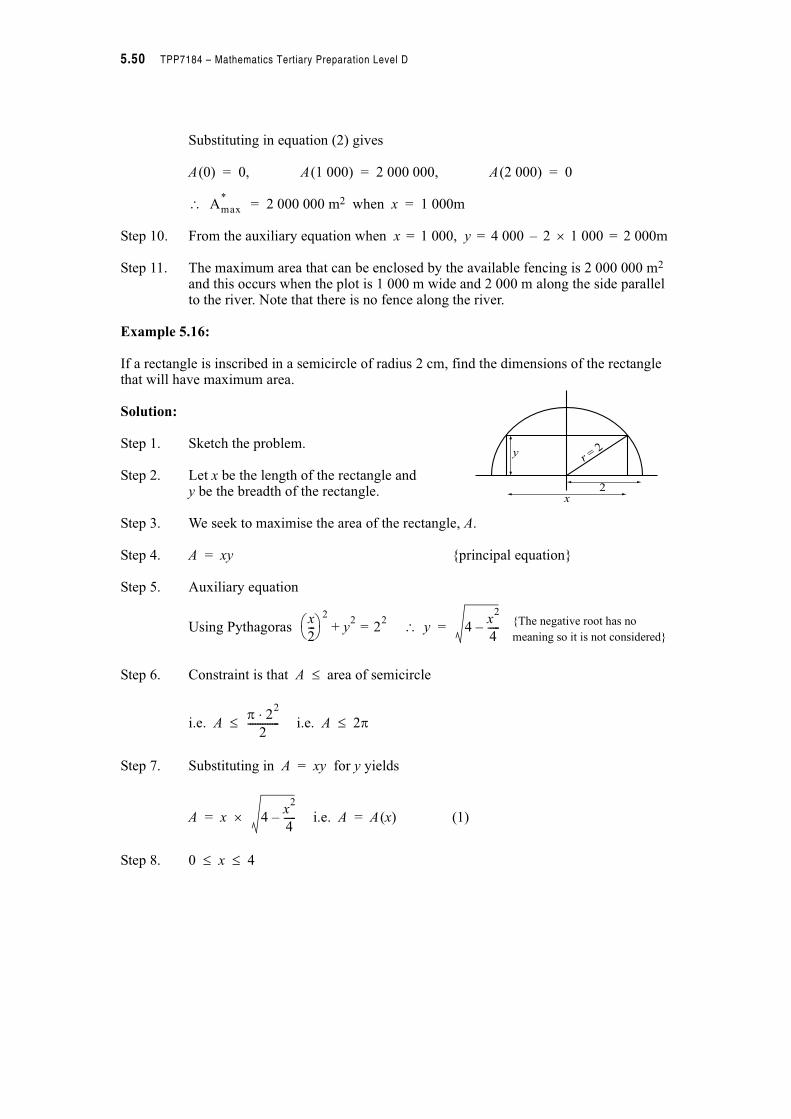
5.50 TPP7184 – Mathematics Tertiary Preparation Level D
Substituting in equation (2) gives
A(0) = 0, A(1 000) = 2 000 000, A(2 000) = 0
= 2 000 000 m2 when x = 1 000m
Step 10. From the auxiliary equation when x = 1 000, y = 4 000 – 2 ! 1 000 = 2 000m
Step 11. The maximum area that can be enclosed by the available fencing is 2 000 000 m2 and this occurs when the plot is 1 000 m wide and 2 000 m along the side parallel to the river. Note that there is no fence along the river.
Example 5.16:
If a rectangle is inscribed in a semicircle of radius 2 cm, find the dimensions of the rectangle that will have maximum area.
Solution:
Step 1. Sketch the problem.
Step 2. Let x be the length of the rectangle andy be the breadth of the rectangle.
Step 3. We seek to maximise the area of the rectangle, A.
Step 4. A = xy {principal equation}
Step 5. Auxiliary equation
Using Pythagoras y ={The negative root has no
meaning so it is not considered}
Step 6. Constraint is that A ' area of semicircle
i.e. A ' i.e. A ' 2)
Step 7. Substituting in A = xy for y yields
A = x ! i.e. A = A(x) (1)
Step 8. 0 ' x ' 4
Amax
*
y
x2
r = 2
x
2---* +, -
2
y2
22
=+ 4x
2
4-----–
) 22.
2-------------
4x
2
4-----–
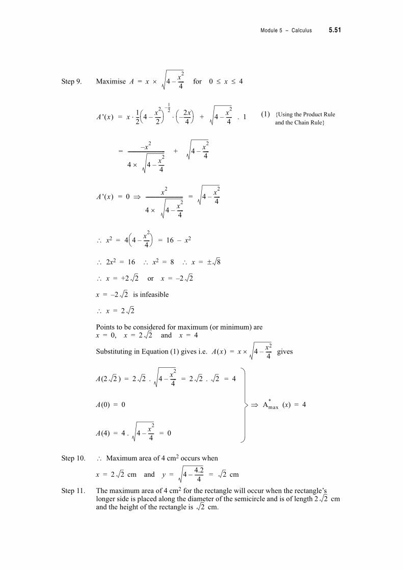
Module 5 – Calculus 5.51
Step 9. Maximise A = x ! for 0 ' x ' 4
= . 1 (1) {Using the Product Rule
and the Chain Rule}
= +
= 0 & =
x2 = = 16 – x2
2x2 = 16 x2 = 8 x =
x = +2 or x = –2
x = –2 is infeasible
x = 2
Points to be considered for maximum (or minimum) arex = 0, x = 2 and x = 4
Substituting in Equation (1) gives i.e. gives
Step 10. Maximum area of 4 cm2 occurs when
x = 2 cm and y = = cm
Step 11. The maximum area of 4 cm2 for the rectangle will occur when the rectangle’s longer side is placed along the diameter of the semicircle and is of length 2 cm and the height of the rectangle is cm.
4x
2
4-----–
A ' x" # x1
2--- 4
x2
2-----–* +
, -1
2---–
2x
4------–* +
, - + 4x
2
4-----–..
x2
–
4 ! 4x
2
4-----–
------------------------------ 4x
2
4-----–
A ' x" #x
2
4 ! 4x
2
4-----–
------------------------------ 4x
2
4-----–
4 4x
2
4-----–* +
, -
8/
2 2
2
2
2
A x" # x 4x2
4-----–!=
A(2 ) = 2 . = 2 . = 4
A(0) = 0 & (x) = 4
A(4) = 4 . = 0
2 2 4x
2
4-----– 2 2
Amax
*
4x
2
4-----–
2 44.2
4-------– 2
22

5.52 TPP7184 – Mathematics Tertiary Preparation Level D
Exercise Set 5.8
1. A farmer has 3 000 metres of fencing available to enclose a rectangular plot. What is the largest area that can be enclosed?
2. What are the dimensions of a closed aluminium can that can hold 4 000 cm3 if the minimum amount of material is to be used in the construction of the can?
3. A 50 kg object is to be dragged along a horizontal surface by a rope making an angle 0 with the horizontal surface.
The force F required to move the object is given by
F = where c is a constant called the coefficient of friction.
Show that the force is maximised or minimised when tan 0 = c
4. A 35 cm length of wire is to be cut into two pieces. One piece will be bent into a square and the other piece will be bent into a circle. How should the wire be cut so that the enclosed area is minimised?
There remains one last topic to cover in the differentiation section of this module. It is a very useful and important technique which uses differentiation to find where a function f(x) equals zero, i.e. to find the roots (or zeros or x-intercepts) of a function.
Usually we have found the root of functions by setting f(x) equal to zero and using an appropriate formula or inverse function .
Recall that:
• For a linear equation, y = ax + b,
When y = 0 $ ax + b = 0 x =
e.g. y = 2x – 6. When y = 0 $ 2x – 6 = 0
x = 3 is the root (or x-intercept)
• For a parabolic equation, y = ax2 + bx + c.
When y = 0 $ x =
e.g. y = –x2 – 3x + 8, When y = 0 $ –x2 – 3x + 8 = 0
x =
x = and x = are the roots (or x-intercepts)
50c
c 0sin" # 0cos+-------------------------------------
b
a---–
b– b2
4ac–/2a
----------------------------------
3–" #– 3–" #2 4 1–" # 8!!–/2 1–" #!
---------------------------------------------------------------------------
3 41+
2–-------------------
3 41–
2–-------------------
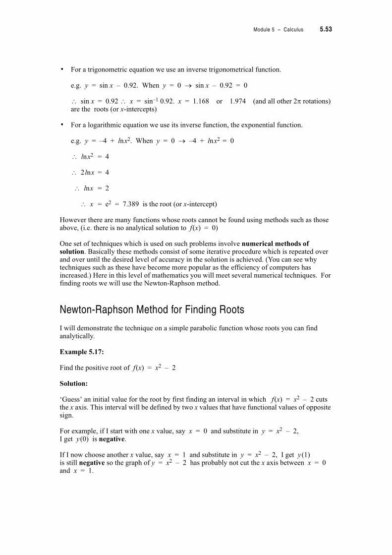
Module 5 – Calculus 5.53
• For a trigonometric equation we use an inverse trigonometrical function.
e.g. y = sin x – 0.92. When y = 0 $ sin x – 0.92 = 0
sin x = 0.92 x = sin–1 0.92. x = 1.168 or 1.974 (and all other 2) rotations) are the roots (or x-intercepts)
• For a logarithmic equation we use its inverse function, the exponential function.
e.g. y = –4 + lnx2. When y = 0 $ –4 + lnx2 = 0
lnx2 = 4
2lnx = 4
lnx = 2
x = e2 = 7.389 is the root (or x-intercept)
However there are many functions whose roots cannot be found using methods such as those above, (i.e. there is no analytical solution to f(x) = 0)
One set of techniques which is used on such problems involve numerical methods of solution. Basically these methods consist of some iterative procedure which is repeated over and over until the desired level of accuracy in the solution is achieved. (You can see why techniques such as these have become more popular as the efficiency of computers has increased.) Here in this level of mathematics you will meet several numerical techniques. For finding roots we will use the Newton-Raphson method.
Newton-Raphson Method for Finding Roots
I will demonstrate the technique on a simple parabolic function whose roots you can find analytically.
Example 5.17:
Find the positive root of f(x) = x2 – 2
Solution:
‘Guess’ an initial value for the root by first finding an interval in which f(x) = x2 – 2 cuts the x axis. This interval will be defined by two x values that have functional values of opposite sign.
For example, if I start with one x value, say x = 0 and substitute in y = x2 – 2,I get y(0) is negative.
If I now choose another x value, say x = 1 and substitute in y = x2 – 2, I get y(1)is still negative so the graph of y = x2 – 2 has probably not cut the x axis between x = 0and x = 1.
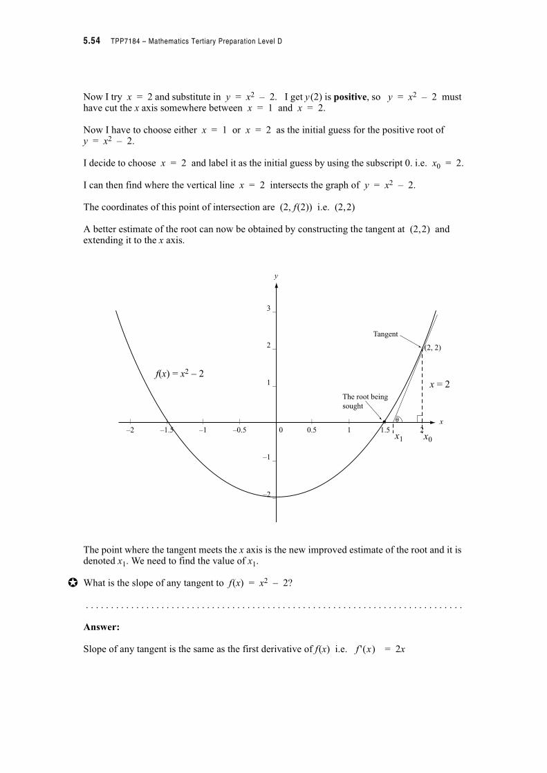
5.54 TPP7184 – Mathematics Tertiary Preparation Level D
Now I try x = 2 and substitute in y = x2 – 2. I get y(2) is positive, so y = x2 – 2 must have cut the x axis somewhere between x = 1 and x = 2.
Now I have to choose either x = 1 or x = 2 as the initial guess for the positive root ofy = x2 – 2.
I decide to choose x = 2 and label it as the initial guess by using the subscript 0. i.e. x0 = 2.
I can then find where the vertical line x = 2 intersects the graph of y = x2 – 2.
The coordinates of this point of intersection are (2, f(2)) i.e. (2,2)
A better estimate of the root can now be obtained by constructing the tangent at (2,2) and extending it to the x axis.
The point where the tangent meets the x axis is the new improved estimate of the root and it is denoted x1. We need to find the value of x1.
What is the slope of any tangent to f(x) = x2 – 2?
. . . . . . . . . . . . . . . . . . . . . . . . . . . . . . . . . . . . . . . . . . . . . . . . . . . . . . . . . . . . . . . . . . . . . . . . . . .
Answer:
Slope of any tangent is the same as the first derivative of f(x) i.e. = 2x
| | | | | | | |
–2 –1.5 –1 –0.5 0 0.5 1 1.5 2
3 _
2 _
1 _
–1 _
–2 _
The root being
sought
x0
x1
(2, 2)
x
y
• θ
Tangent
f(x) = x2 – 2x = 2
x1 x0
f ' x !
Module 5 – Calculus 5.55
What is the slope of the tangent at (2,2)? . . . . . . . . . . . . . . . . . . . . . . . . . . . . . . . . . . . . . . . . .
Answer:
Slope at (2,2) is
= 2 " 2 = 4
What is the y coordinate corresponding to x1? . . . . . . . . . . . . . . . . . . . . . . . . . . . . . . . . . . . . . .
Answer:
The y coordinate is zero (because x1 is on the x axis)
Find tan # from the two points (2,2) and (x1,0) . . . . . . . . . . . . . . . . . . . . . . . . . . . . . . . . . . . .
Answer:
tan # =
What other value gives tan #? . . . . . . . . . . . . . . . . . . . . . . . . . . . . . . . . . . . . . . . . . . . . . . . . . . .
Answer:
The derivative (which we know is 4).
So now we have two expressions for tan # which we can equate and solve for x1.
= 4
$ –2 = 4(x1 – 2)
$ = x1 – 2
$ x1 = 2 – See Note 1
= 1.5
Notes
1. The new estimate of the root equals the old estimate of the root minus the functional value at the old estimate divided
by value of the derivative for the old estimate.
i.e.
f ' 2 !
f ' 2 !
0 2–
x1 2–-------------
f ' 2 !
0 2–
x1 2–-------------
2–
4------
2
4---
x1 x0
f x0 !
f ' x0 !-------------–=
5.56 TPP7184 – Mathematics Tertiary Preparation Level D
Now to get an even better estimate of the root we will repeat the procedure. (I’ll give you the instructions and you do the drawing, etc. on the graph opposite.)
Draw a line from x1 = 1.5 to the curve.
What are the coordinates of the point of intersection? (1.5,0.25)
Draw a tangent to the curve at (1.5,0.25)
Extend this line to cut the x axis.
Label where the line cuts the x axis as x2. (This is the new, more improved estimate of the root.)
What is the y coordinate corresponding to x2?
Mark the angle the line made with x axis as #2.
Now we can find two expressions for tan #2.
tan #2 = evaluated at x1 = 1.5 i.e. tan #2 = = 2 " 1.5 = 3
and tan #2 =
$ 3 =
$ x2 = 1.5 –
= 1.41667
You should be able to see that we can again repeat the process and get an even better estimation of the root. This iterative process is typical of numerical methods. The next thing to address is when to stop the iterations!!!!
We need to develop some stopping criterion. For example, ‘accurate to 3 decimal places’.
So we have not reached the desired accuracy and we need to do more iterations. But this time instead of repeating all the steps, we’ll use an iterative formula.
f ' x ! f ' 1.5 !
0 0.25–
x2 1.5–-------------------
0 0.25–
x2 1.5–-------------------
0.25
3---------- i.e. x2 x1
f x1 !f ' x1 !------------–=
% &' () *
So far we have x0 = 2
x1 = 1.5 $ x1 + x0 to 3 decimal places
x2 = 1.41667 $ x2 + x1 to 3 decimal places

Module 5 – Calculus 5.57
We have shown that x1 = x0 –
and x2 = x1 –
In general
Do not proceed with this if you are not convinced the iterative formula will work.$ To find x3 we can use the general formula
x3 = x2 –
Now x2 = 1.41667 $ f(x2) = f(1.41667) = 1.416672 – 2 = 0.006954
and = = 2 " 1.41667 = 2.83334
$ x3 = 1.41667 –
= 1.41422
Now check the stopping criterion. ‘Is x3 = x2 to 3 decimal places?’
x2 = 1.41667
x3 = 1.41422 $ x3 + x2 to 3 decimal places
So another iteration is required. For convenience let’s summarise the iterations in a table.
f x0 !f ' x0 !------------
f x1 !f ' x1 !------------
xn 1+ xn
f xn !
f, xn !-------------–=
f x2 !f ' x2 !------------
f ' x2 ! f ' 1.41667 !
0.006954
2.83334----------------------
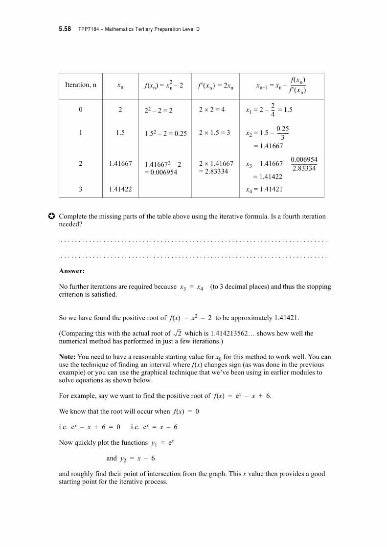
5.58 TPP7184 – Mathematics Tertiary Preparation Level D
Complete the missing parts of the table above using the iterative formula. Is a fourth iteration needed?
. . . . . . . . . . . . . . . . . . . . . . . . . . . . . . . . . . . . . . . . . . . . . . . . . . . . . . . . . . . . . . . . . . . . . . . . . . .
. . . . . . . . . . . . . . . . . . . . . . . . . . . . . . . . . . . . . . . . . . . . . . . . . . . . . . . . . . . . . . . . . . . . . . . . . . .
Answer:
No further iterations are required because x3 = x4 (to 3 decimal places) and thus the stopping criterion is satisfied.
So we have found the positive root of f(x) = x2 – 2 to be approximately 1.41421.
(Comparing this with the actual root of which is 1.414213562… shows how well the numerical method has performed in just a few iterations.)
Note: You need to have a reasonable starting value for x0 for this method to work well. You can use the technique of finding an interval where f(x) changes sign (as was done in the previous example) or you can use the graphical technique that we’ve been using in earlier modules to solve equations as shown below.
For example, say we want to find the positive root of f(x) = ex – x + 6.
We know that the root will occur when f(x) = 0
i.e. ex – x + 6 = 0 i.e. ex = x – 6
Now quickly plot the functions y1 = ex
and y2 = x – 6
and roughly find their point of intersection from the graph. This x value then provides a good starting point for the iterative process.
Iteration, n xn f(xn) = = 2xn xn+1 = xn –
0 2 22 – 2 = 2 2 " 2 = 4 x1 = 2 – = 1.5
1 1.5 1.52 – 2 = 0.25 2 " 1.5 = 3 x2 = 1.5 –
= 1.41667
2 1.41667 1.416672 – 2= 0.006954
2 " 1.41667= 2.83334
x3 = 1.41667 –
= 1.41422
3 1.41422 x4 = 1.41421
xn
22– f ' xn !
f xn !
f ' xn !-------------
2
4---
0.25
3----------
0.006954
2.83334----------------------
2
Module 5 – Calculus 5.59
Exercise Set 5.9
Use the Newton-Raphson numerical technique to solve each of the following. Check your solutions.1. Find the positive root of f(x) = ex + x – 3 accurate to 2 decimal places.
2. Find the roots of the following equations accurate to 2 decimal places.
(a) y = lnx + x – 2
(b) y = e2x – x2 – 10
3. (i) Show that f(x) = x4 – x3 – 75 has a root between x = 3 and x = 4
(ii) Find the root accurate to 5 decimal places
4. Find the point of intersection of f(x) = cos x and f(x) = x accurate to 5 decimal places.
5. Find the lowest solution, accurate to 4 decimal places of –x2 + 1 = sin x.
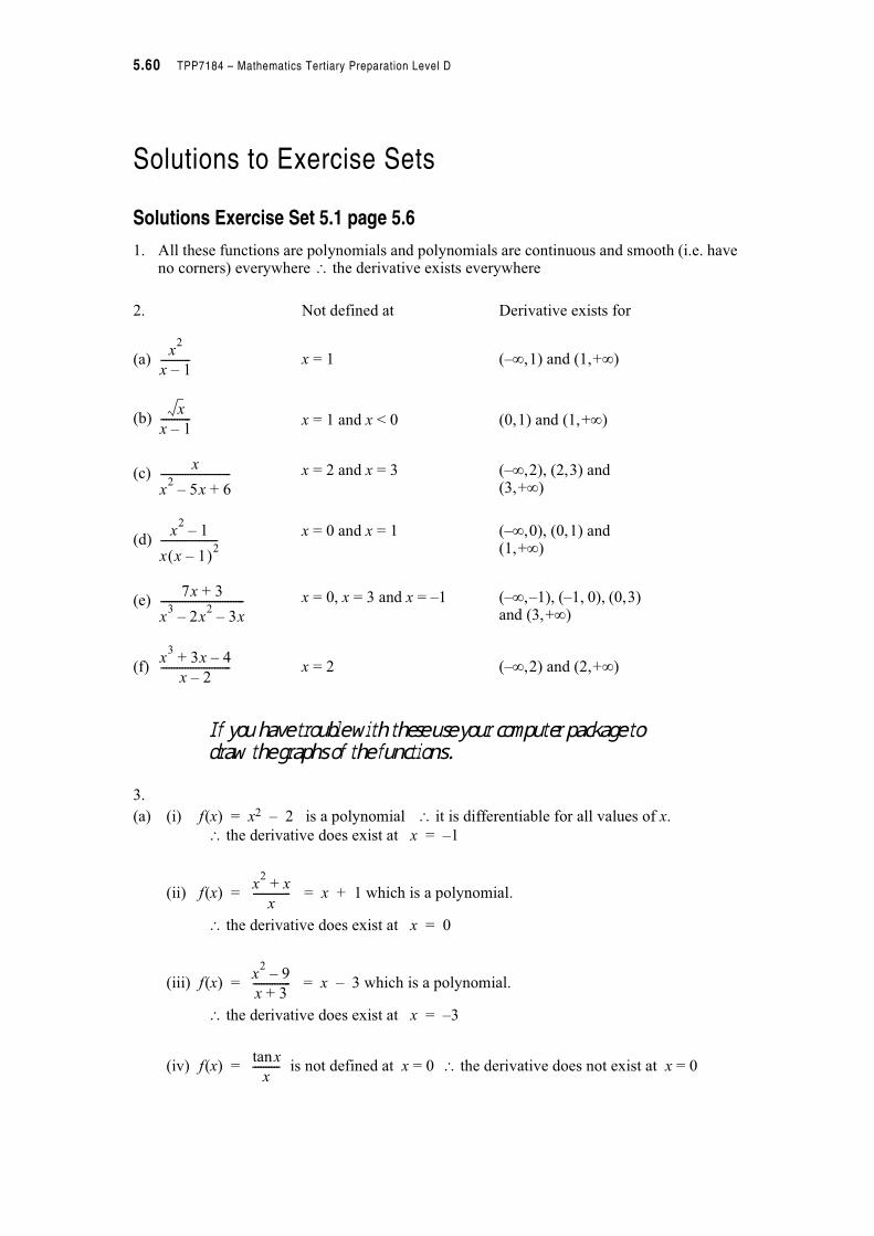
5.60 TPP7184 – Mathematics Tertiary Preparation Level D
Solutions to Exercise Sets
Solutions Exercise Set 5.1 page 5.6
1. All these functions are polynomials and polynomials are continuous and smooth (i.e. have no corners) everywhere $ the derivative exists everywhere
If you have trouble with these use your computer package to draw the graphs of the functions.3.
(a) (i) f(x) = x2 – 2 is a polynomial $ it is differentiable for all values of x.
$ the derivative does exist at x = –1
(ii) f(x) = = x + 1 which is a polynomial.
$ the derivative does exist at x = 0
(iii) f(x) = = x – 3 which is a polynomial.
$ the derivative does exist at x = –3
(iv) f(x) = is not defined at x = 0 $ the derivative does not exist at x = 0
2. Not defined at Derivative exists for
(a) x = 1 (–-,1) and (1,+-)
(b) x = 1 and x < 0 (0,1) and (1,+-)
(c) x = 2 and x = 3 (–-,2), (2,3) and (3,+-)
(d)x = 0 and x = 1 (–-,0), (0,1) and
(1,+-)
(e) x = 0, x = 3 and x = –1 (–-,–1), (–1, 0), (0,3) and (3,+-)
(f) x = 2 (–-,2) and (2,+-)
x2
x 1–-----------
x
x 1–-----------
x
x2
5x 6+–--------------------------
x2
1–
x x 1– !2---------------------
7x 3+
x3
2x2
3x––-------------------------------
x3
3x 4–+
x 2–--------------------------
x2
x+
x--------------
x2
9–
x 3+--------------
xtan
x----------
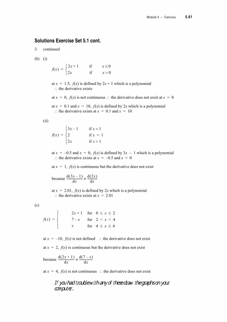
Module 5 – Calculus 5.61
Solutions Exercise Set 5.1 cont.
3. continued
(b) (i)
at x = 1.5, f(x) is defined by 2x + 1 which is a polynomial
$ the derivative exists
at x = 0, f(x) is not continuous $ the derivative does not exist at x = 0
at x = 0.1 and x = 10, f(x) is defined by 2x which is a polynomial
$ the derivative exists at x = 0.1 and x = 10
(ii)
at x = –0.5 and x = 0, f(x) is defined by 3x – 1 which is a polynomial
$ the derivative exists at x = –0.5 and x = 0
at x = 1, f(x) is continuous but the derivative does not exist
because
at x = 2.01, f(x) is defined by 2x which is a polynomial
$ the derivative exists at x = 2.01
(c)
at x = –10, f(x) is not defined $ the derivative does not exist
at x = 2, f(x) is continuous but the derivative does not exist
because
at x = 4, f(x) is not continuous $ the derivative does not exist
If you had trouble with any of these draw the graphs on your computer.
f x !2x 1+ if x 0.
2x if x 0/%')
=
f x !
3x 1–
2
2x%0'0)
=
if x 11
if x 1=
if x 1/
d 3x 1– !dx
-----------------------d 2x !
dx--------------+
f x !
2x 1+
7 x–
x%0'0)
=
for 0 . x . 2
for 2 < x < 4
for 4 . x . 6
d 2x 1+ !dx
-----------------------d 7 x– !
dx-------------------+
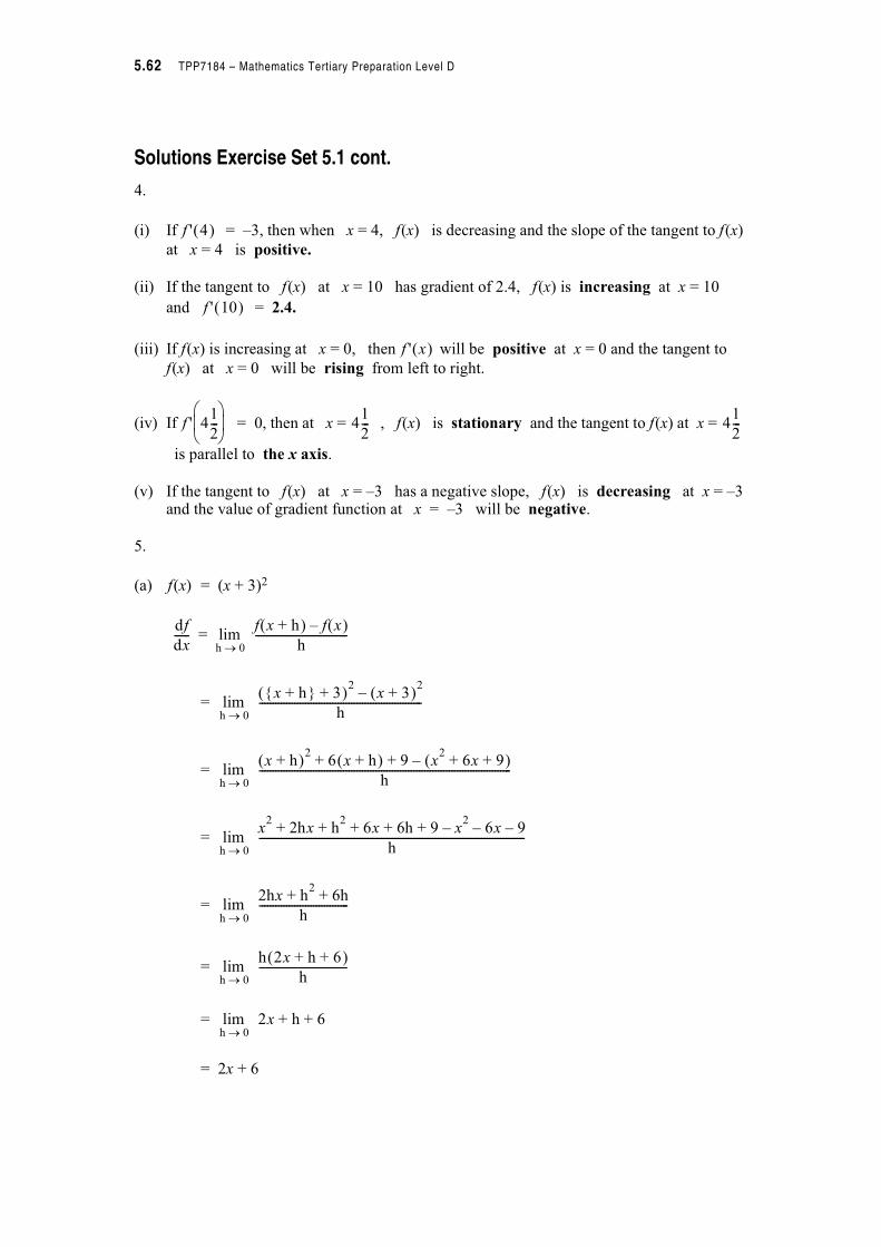
5.62 TPP7184 – Mathematics Tertiary Preparation Level D
Solutions Exercise Set 5.1 cont.
4.
(i) If = –3, then when x = 4, f(x) is decreasing and the slope of the tangent to f(x)
at x = 4 is positive.
(ii) If the tangent to f(x) at x = 10 has gradient of 2.4, f(x) is increasing at x = 10
and = 2.4.
(iii) If f(x) is increasing at x = 0, then will be positive at x = 0 and the tangent to
f(x) at x = 0 will be rising from left to right.
(iv) If = 0, then at x = , f(x) is stationary and the tangent to f(x) at x =
is parallel to the x axis.
(v) If the tangent to f(x) at x = –3 has a negative slope, f(x) is decreasing at x = –3 and the value of gradient function at x = –3 will be negative.
5.
(a) f(x) = (x + 3)2
=
=
=
=
=
=
= 2x + 6
f ' 4 !
f ' 10 !
f ' x !
f ' 41
2---
2 34 56 7
41
2--- 4
1
2---
df
dx------
h 08lim
f x h+ ! f x !–
h----------------------------------=
h 08lim
x h+9 : 3+ !2x 3+ !2
–
h------------------------------------------------------------
h 08lim
x h+ !26 x h+ ! 9 x
26x 9+ + !–+ +
h---------------------------------------------------------------------------------------------
h 08lim
x2
2hx h2
6x 6h 9 x2
6x 9–––+ + + + +
h--------------------------------------------------------------------------------------------------
h 08lim
2hx h2
6h+ +
h---------------------------------
h 08lim
h 2x h 6+ + !h
---------------------------------
h 08lim 2x h 6+ +
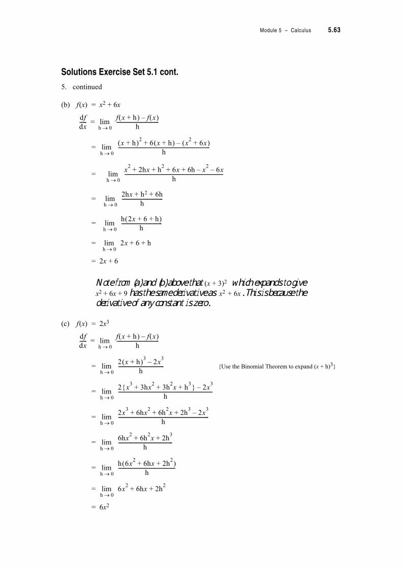
Module 5 – Calculus 5.63
Solutions Exercise Set 5.1 cont.
5. continued
(b) f(x) = x2 + 6x
=
=
=
=
=
= 2x + 6
Note from (a) and (b) above that (x + 3)2 which expands to give x2 + 6x + 9 has the same derivative as x2 + 6x. This is because the derivative of any constant is zero.
(c) f(x) = 2x3
= {Use the Binomial Theorem to expand (x + h)3}
=
=
=
=
=
= 6x2
df
dx------
h 08lim
f x h+ ! f x !–
h----------------------------------=
x h+ !26 x h+ ! x
26x+ !–+
h--------------------------------------------------------------------------
h 08lim
h 08lim
x2
2hx h2
6x 6h x2
6x––+ + + +
h--------------------------------------------------------------------------------
h 08lim
2hx h2 6h+ +
h---------------------------------
h 08lim
h 2x 6 h+ + !h
---------------------------------
h 08lim 2x 6 h+ +
df
dx------
h 08lim
f x h+ ! f x !–
h----------------------------------=
h 08lim
2 x h+ !32x
3–
h-------------------------------------
h 08lim
2 x3
3hx2
3h2x h
3+ + +9 : 2x
3–
h----------------------------------------------------------------------------
h 08lim
2x3
6hx2
6h2x 2h
32x
3–+ + +
h-------------------------------------------------------------------------
6hx2
6h2x 2h
3+ +
h--------------------------------------------
h 08lim
h 08lim
h 6x2
6hx 2h2
+ + !h
----------------------------------------------
h 08lim 6x
26hx 2h
2+ +
5.64 TPP7184 – Mathematics Tertiary Preparation Level D
Solutions Exercise Set 5.1 cont.
5. continued
(d) f(x) =
=
=
=
=
=
=
=
which you may care to write as –3x–2
3
x---
df
dx------
h 08lim
f x h+ ! f x !–
h----------------------------------=
3
x h+------------
3
x---–
h------------------------------------
h 08lim
h 08lim
3 x" 3 x h+ !"–
x x h+ !--------------------------------------------
h---------------------------------------------------------------
Putting fractions in numerator on a9
common denominator:
3x 3x 3h––
x x h+ !------------------------------
h-------------------------------------------
h 08lim
3h–
x2
hx+-----------------
h------------------------------------
h 08lim
3h–
h x2
hx+ !-------------------------
h 08lim
3–
x2
hx+-----------------
h 08lim
3–
x2
------

Module 5 – Calculus 5.65
Solutions Exercise Set 5.2 page 5.11
1.
(a) f(x) = (x + 3)2 = x2 + 6x + 9 i.e. sum of three functions $ find derivative of
each function and then add the derivatives.
=
= 2x2–1 + + 0
= 2x + 6 " 1
= 2x + 6 as found from first principles ✓
(b) f(x) = x2 + 6x
=
= 2x + 6 ✓
(c) f(x) = 2x3
=
= 2 " 3x2
= 6x2 ✓
(d) f(x) = = 3x–1
=
= 3 " (–1)x–1–1
= –3x–2 or ✓
f ' x !dx
2
dx--------
d6x
dx---------
d9
dx------+ +
6dx
dx------
f ' x !dx
2
dx-------- 6
dx
dx------+
f ' x ! 2dx
3
dx--------
3
x--- 3
1
x---"
2 36 7=
f ' x ! 3dx
1–
dx----------
3–
x2
------
5.66 TPP7184 – Mathematics Tertiary Preparation Level D
Solutions Exercise Set 5.2 cont.
2.
(a) f(x) = 6log x + 4 {log x means log to the base 10 of x}
= {Take care here, x + 4 is not bracketed so the log applies only to x}
= + 0
=
=
(b) f(x) = 8ex – ln x
=
= 8ex –
(c) f(x) = + ln x2 + 1
=
We do not know how to find the derivative of a ‘complicated’ function like ln x2.
(ln x2 is a function of a function because it is a natural log function of a quadratic function.)
So we need to think about changing ln x2 into another form.
f ' x ! 6d xlog
dx--------------
d4
dx------+
61
ln10 x"--------------------"
6
ln10 !x-------------------
2.6058
x----------------
f ' x ! 8de
x
dx-------
dlnx
dx-----------–
1
x---
1
x---
f ' x !d
1
x---
dx------
d lnx2
dx-----------------
d1
dx------+ +
Module 5 – Calculus 5.67
Solutions Exercise Set 5.2 cont.
2. continued
From the logarithm rules we know ln xa = a ln x
$ ln x2 = 2 ln x
$ =
=
=
=
(d) f(x) = ; – cos x + 8tan x +
=
= 0 – (–sin x) + 8sec2 x + " 2x {Note: ; is a constant $ its derivative is zero}
= sin x + 8sec2 x +
Note: If you want to evaluate f(x) or at a particular x value, you must have the calculator in radian mode.
(e) f(x) = 3x – 3ex + 3 + e
= + 0 + 0 {e is a constant $ its derivative is zero}
= ln 3 " 3x – 3ex
= 1.0986 " 3x – 3ex
f ' x !d
1
x---
dx------
d2lnx
dx--------------
d1
dx------+ +
1–
x2
------2dlnx
dx-------------- 0+ +
1–
x2
------ 21
x---"+
1–
x2
------2
x---+
x2
6-----
f ' x !d;dx------
d xcos
dx--------------
8d xtan
dx-----------------
1
6---
dx2
dx--------+ +–
1
6---
x
3---
f ' x !
f ' x !d3
x
dx--------
3dex
dx----------–
5.68 TPP7184 – Mathematics Tertiary Preparation Level D
Solutions Exercise Set 5.2 cont.
3. Gradient of the tangent to f(x) at some point a, is the derivative evaluated at a.
As you do each of these examine and think about what it tells you about the behaviour of f(x) at x = a.(a) f(x) = 3x2 – 4x + 2
= 6x – 4
$ = 6 " (–2) – 4 = –12 – 4 = –16
(b) f(x) = 8 lnx
=
$ =
(c) f(x) = ex – x
= ex – 1
= e–1–1 = –0.632
(d) f(x) =
= + 10x–1
= – 10x–2
$ = – 10 " 3–2
= –0.8224
f ' x !
f ' a !
f ' x !
f ' 2– !
f ' x !8
x---
f ' 4 !8
4--- 2=
f ' x !
f ' 1– !
x10
x------+
x
1
2---
f ' x !1
2---x
1–
2------
f ' 3 !1
2--- 3
1–
2------
"
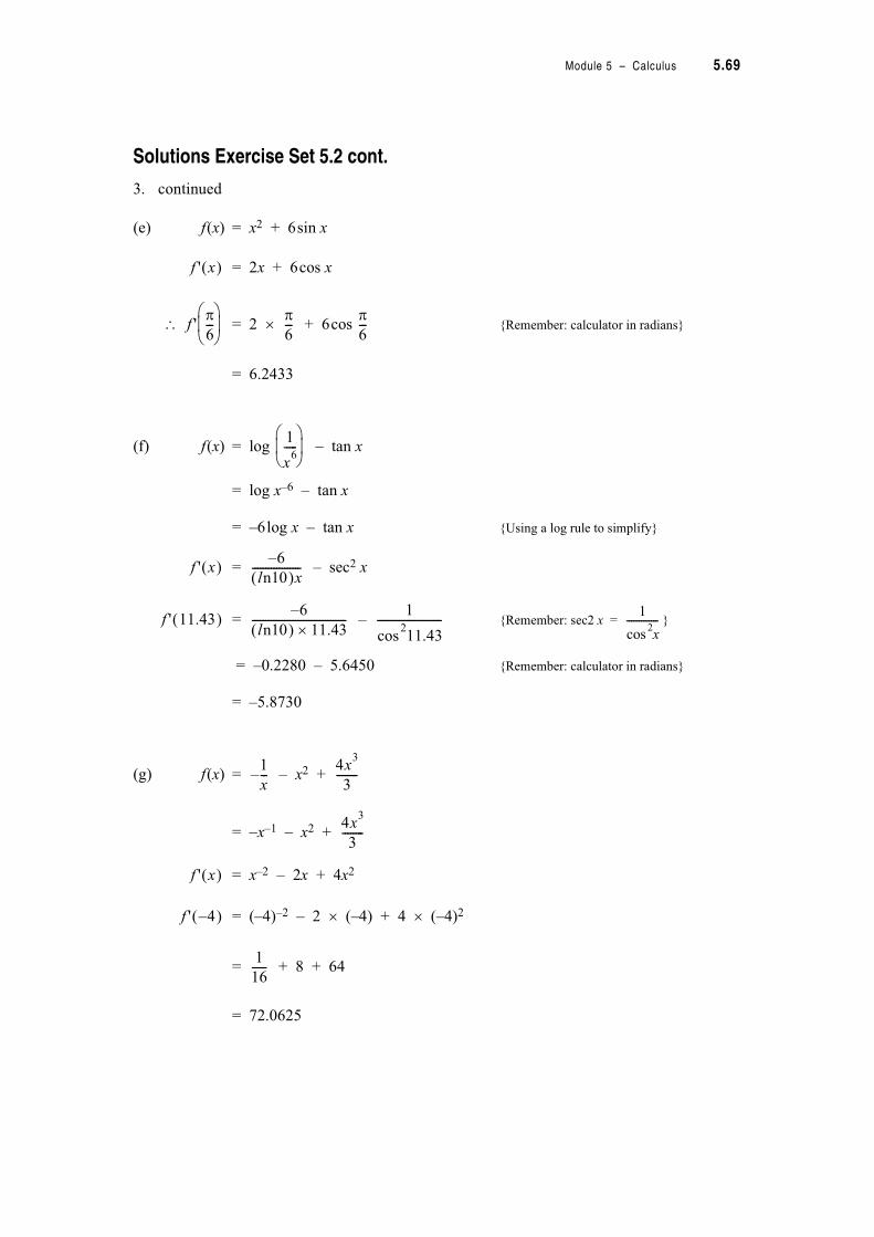
Module 5 – Calculus 5.69
Solutions Exercise Set 5.2 cont.
3. continued
(e) f(x) = x2 + 6sin x
= 2x + 6cos x
$ = 2 " + 6cos {Remember: calculator in radians}
= 6.2433
(f) f(x) = log – tan x
= log x–6 – tan x
= –6log x – tan x {Using a log rule to simplify}
= – sec2 x
= – {Remember: sec2 x = }
= –0.2280 – 5.6450 {Remember: calculator in radians}
= –5.8730
(g) f(x) = – x2 +
= –x–1 – x2 +
= x–2 – 2x + 4x2
= (–4)–2 – 2 " (–4) + 4 " (–4)2
= + 8 + 64
= 72.0625
f ' x !
f ';6---
2 34 56 7 ;
6---
;6---
1
x6
-----2 34 56 7
f ' x !6–
ln10 !x------------------
f ' 11.43 !6–
ln10 ! 11.43"-----------------------------------
1
11.432
cos------------------------
1
x2
cos-------------
1
x---–
4x3
3--------
4x3
3--------
f ' x !
f ' 4– !
1
16------
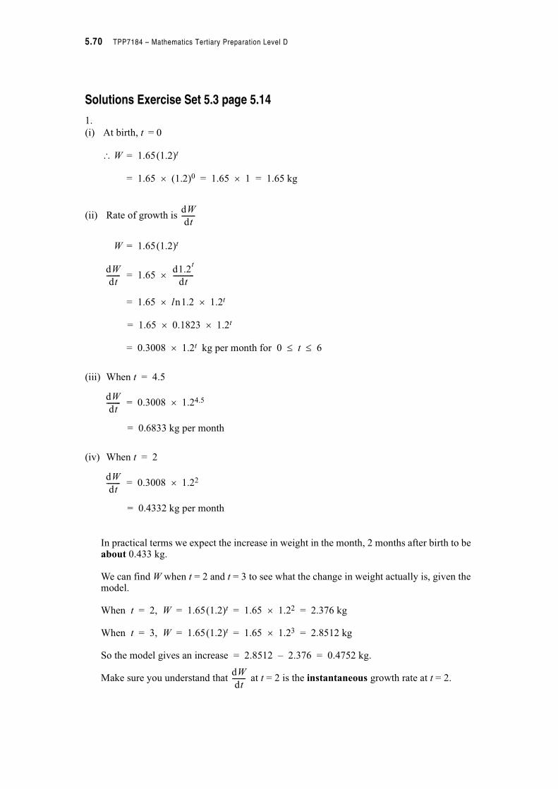
5.70 TPP7184 – Mathematics Tertiary Preparation Level D
Solutions Exercise Set 5.3 page 5.14
1.
(i) At birth, t = 0
$ W = 1.65(1.2)t
= 1.65 " (1.2)0 = 1.65 " 1 = 1.65 kg
(ii) Rate of growth is
W = 1.65(1.2)t
= 1.65 "
= 1.65 " ln1.2 " 1.2t
= 1.65 " 0.1823 " 1.2t
= 0.3008 " 1.2t kg per month for 0 . t . 6
(iii) When t = 4.5
= 0.3008 " 1.24.5
= 0.6833 kg per month
(iv) When t = 2
= 0.3008 " 1.22
= 0.4332 kg per month
In practical terms we expect the increase in weight in the month, 2 months after birth to be about 0.433 kg.
We can find W when t = 2 and t = 3 to see what the change in weight actually is, given the model.
When t = 2, W = 1.65(1.2)t = 1.65 " 1.22 = 2.376 kg
When t = 3, W = 1.65(1.2)t = 1.65 " 1.23 = 2.8512 kg
So the model gives an increase = 2.8512 – 2.376 = 0.4752 kg.
Make sure you understand that at t = 2 is the instantaneous growth rate at t = 2.
dW
dt--------
dW
dt--------
d1.2t
dt------------
dW
dt--------
dW
dt--------
dW
dt--------
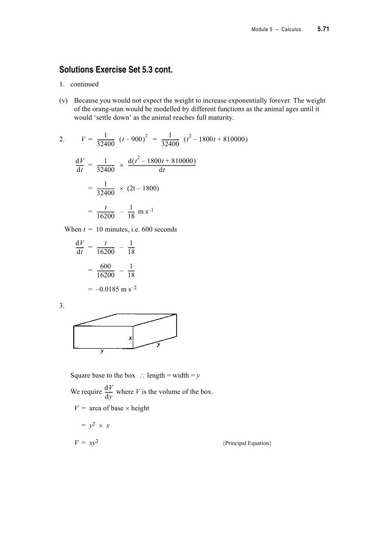
Module 5 – Calculus 5.71
Solutions Exercise Set 5.3 cont.
1. continued
(v) Because you would not expect the weight to increase exponentially forever. The weight
of the orang-utan would be modelled by different functions as the animal ages until it
would ‘settle down’ as the animal reaches full maturity.
2. V = =
= "
= " (2t – 1800)
= – m s–1
When t = 10 minutes, i.e. 600 seconds
= –
= –
= –0.0185 m s–2
3.
Square base to the box $ length = width = y
We require where V is the volume of the box.
V = area of base " height
= y2 " x
V = xy2 {Principal Equation}
1
32400--------------- t 900– !2 1
32400--------------- t
21800t 810000+– !
dV
dt-------
1
32400---------------
d t2
1800t– 810000+ !dt
--------------------------------------------------------
1
32400---------------
t
16200---------------
1
18------
dV
dt-------
t
16200---------------
1
18------
600
16200---------------
1
18------
dV
dy-------
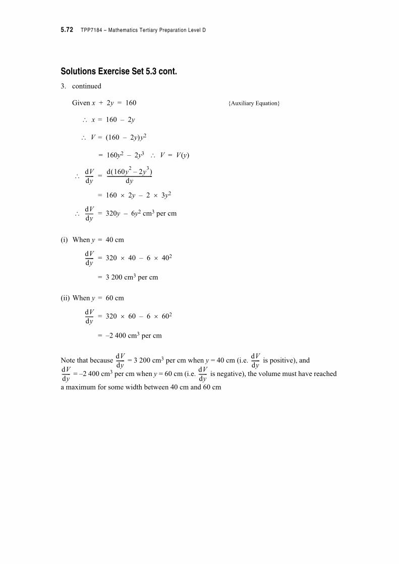
5.72 TPP7184 – Mathematics Tertiary Preparation Level D
Solutions Exercise Set 5.3 cont.
3. continued
Given x + 2y = 160 {Auxiliary Equation}
$ x = 160 – 2y
$ V = (160 – 2y)y2
= 160y2 – 2y3 $ V = V(y)
$ =
= 160 " 2y – 2 " 3y2
$ = 320y – 6y2 cm3 per cm
(i) When y = 40 cm
= 320 " 40 – 6 " 402
= 3 200 cm3 per cm
(ii) When y = 60 cm
= 320 " 60 – 6 " 602
= –2 400 cm3 per cm
Note that because = 3 200 cm3 per cm when y = 40 cm (i.e. is positive), and
= –2 400 cm3 per cm when y = 60 cm (i.e. is negative), the volume must have reached
a maximum for some width between 40 cm and 60 cm
dV
dy-------
d 160y2
2y3
– !dy
-------------------------------------
dV
dy-------
dV
dy-------
dV
dy-------
dV
dy-------
dV
dy-------
dV
dy-------
dV
dy-------
Module 5 – Calculus 5.73
Solutions Exercise Set 5.3 cont.
4.
(i) s = 60t2(3 – 2t) = 180t2 – 120t3
is required as is the velocity, V in km h–1
V = =
= 360t – 360t2 km h–1
(ii) Acceleration, a = and the units will be km h–2
=
= 360 – 720t km h–2
(iii) When t = 20 minutes = hour
V = 360t – 360t2
= 360 " – 360 "
= 80 km h–1
a = 360 – 720t
= 360 – 720 "
= 120 km h–2
ds
dt-----
ds
dt-----
ds
dt-----
d 180t2
120t3
– !dt
-----------------------------------------
dV
dt-------
adV
dt-------=
d 360t 360t2
–
dt-------------------------------------
1
3---
1
3---
1
3---2 3
6 72
1
3---
5.74 TPP7184 – Mathematics Tertiary Preparation Level D
Solutions Exercise Set 5.3 cont.
5. Slope of tangent at equals the derivative, at x =
= 2 – (–3sin x) = 2 + 3sin x
When x =
= 2 + 3sin x = 2 + 3sin {Remember: Radian mode for calculator}
= 2 + 3 " 1 = 5
General equation to a straight line is y = mx + c
slope m = 5
$ y = 5x + c
lies on the tangent line
$ ; = 5 " + c
$ c =
$ Equation of tangent at is
y = 5x –
;2--- ;<
2 34 56 7 dy
dx------
;2---
dy
dx------
;2---
dy
dx------
;2---
;2--- ;<
2 34 56 7
;2---
3;–
2---------
;2--- ;<
2 34 56 7
3;2
------
Module 5 – Calculus 5.75
Solutions Exercise Set 5.4 page 5.23
1.
(a) y = (x2 + 2) (2x – 4)
y is the product of two functions of x so the product rule is needed.
= = +
Let u(x) = x2 + 2 and v(x) = 2x – 4
$ = 2x and = 2
= +
= (2x – 4) " 2x + (x2 + 2) " 2
= 4x2 – 8x + 2x2 + 4
= 6x2 – 8x + 4
Checking: y = (x2 + 2) (2x – 4) = 2x3 – 4x2 + 4x – 8
$ = 6x2 – 8x + 4 ✓
(b) y = cos x . sin x
= = +
Let u(x) = cos x and v(x) = sin x
$ = –sin x and = cos x
= +
= sin x " (–sin x) + cos x " cos x
= cos2 x – sin2 x
dy
dx------
du v=dx
------------- vdu
dx------= u
dv
dx------=
du
dx------
dv
dx------
du v=dx
------------- vdu
dx------= u
dv
dx------=
dy
dx------
dy
dx------
du v=dx
------------- vdu
dx------= u
dv
dx------=
du
dx------
dv
dx------
dy
dx------ v
du
dx------= u
dv
dx------=
5.76 TPP7184 – Mathematics Tertiary Preparation Level D
Solutions Exercise Set 5.4 cont.
1. continued
(c) f(x) = lnx
= = +
Let u(x) = = 3x–1 and v(x) = lnx
$ = –3x–2 and =
= +
= lnx " (–3x–2) + "
= +
=
(d) y = 3x tan x
= = +
Let u(x) = 3x and v(x) = tan x
$ = ln3 " 3x and = sec2 x
= tan x " ln3 " 3x + 3x " sec2 x
= ln3 . 3x tan x + 3x sec2 x
3
x---
df
dx------
du v=dx
------------- vdu
dx------= u
dv
dx------=
3
x---
du
dv------
dv
dx------
1
x---
du v=dx
------------- vdu
dx------= u
dv
dx------=
3
x---
1
x---
3– lnx
x2
--------------3
x2
-----
3 3lnx–
x2
--------------------
dy
dx------
du v=dx
------------- vdu
dx------= u
dv
dx------=
du
dx------
dv
dx------
du v=dx
-------------

Module 5 – Calculus 5.77
Solutions Exercise Set 5.4 cont.
1. continued
(e) z = e2x
z is a function of a function. (The ‘exponential to base e’ function of the ‘2 times x’ function.)
To use the product rule we must write e2x as the product of two functions of x.
z = e2x = ex . ex {Remember the index rule am . an = am+n}
= +
Let u(x) = ex and v(x) = ex
$ = ex and = ex
= +
= ex . ex + ex . ex
= e2x + e2x
= 2e2x
Here is a new rule which you need to add to the table of derivatives you should know.
dz
dx------ v
du
dx------= u
dv
dx------=
du
dx------
dv
dx------
du v=dx
------------- vdu
dx------= u
dv
dx------=
where k is a constantde
kx
dx---------- ke
kx=

5.78 TPP7184 – Mathematics Tertiary Preparation Level D
Solutions Exercise Set 5.4 cont.
1. continued
(f) y = = = Note: is function of a function which is
why I have rewritten it as the product
= = +
Let u(x) = and v(x) =
=
$ = " –1 " x–2
= $ =
= +
= +
=
=
x1–
4-------
2 34 56 7 2
1
4x------
2 34 56 7 2
1
4x------
1
4x------= x
1–
4-------
2 34 56 7
2
1
4x------
1
4x------=
dy
dx------
du v=dx
------------- vdu
dx------= u
dv
dx------=
1
4x------
1
4x------
1
4--- x
1–=
du
dx------
1
4---
1–
4x2
--------dv
dx------
1–
4x2
--------
du v=dx
------------- vdu
dx------= u
dv
dx------=
1
4x------
1–
4x2
--------=1
4x------
1–
4x2
--------=
2–
16x3
-----------
1–
8x3
--------
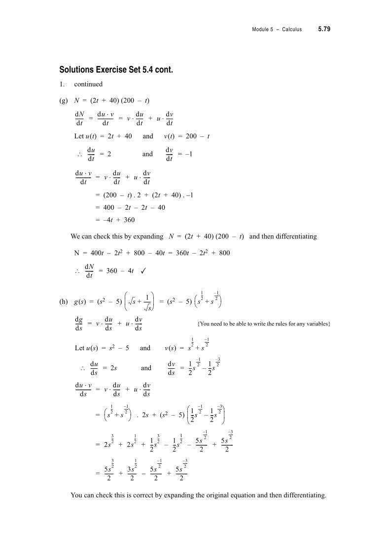
Module 5 – Calculus 5.79
Solutions Exercise Set 5.4 cont.
1. continued
(g) N = (2t + 40) (200 – t)
= = +
Let u(t) = 2t + 40 and v(t) = 200 – t
$ = 2 and = –1
= +
= (200 – t) . 2 + (2t + 40) . –1
= 400 – 2t – 2t – 40
= –4t + 360
We can check this by expanding N = (2t + 40) (200 – t) and then differentiating
N = 400t – 2t2 + 800 – 40t = 360t – 2t2 + 800
$ = 360 – 4t ✓
(h) g(s) = (s2 – 5) = (s2 – 5)
= + {You need to be able to write the rules for any variables}
Let u(s) = s2 – 5 and v(s) =
$ = 2s and =
= +
= . 2s + (s2 – 5)
= + + – – +
= + – +
You can check this is correct by expanding the original equation and then differentiating.
dN
dt-------
du v=dt
------------- vdu
dt------= u
dv
dt------=
du
dt------
dv
dt------
du v=dt
------------- vdu
dt------= u
dv
dt------=
dN
dt-------
s1
s------+
2 34 56 7
s
1
2---
s
1–
2------
+2 36 7
dg
ds------ v
du
ds------= u
dv
ds------=
s
1
2---
s
1–
2------
+
du
ds------
dv
ds------
1
2---s
1–
2------ 1
2---s
3–
2------
–
du v=ds
------------- vdu
ds------= u
dv
ds------=
s
1
2---
s
1–
2------
+2 36 7 1
2---s
1–
2------ 1
2---s
3–
2------
–2 34 56 7
2s
3
2---
2s
1
2--- 1
2---s
3
2--- 1
2---s
12--- 5s
1–
2------
2----------
5s
3–
2------
2----------
5s
3
2---
2-------
3s
1
2---
2-------
5s
1–
2------
2----------
5s
3–
2------
2----------
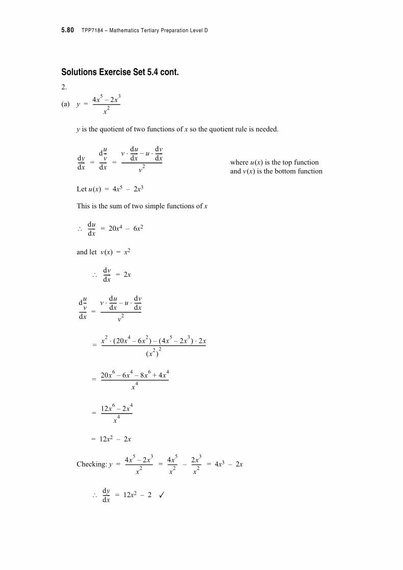
5.80 TPP7184 – Mathematics Tertiary Preparation Level D
Solutions Exercise Set 5.4 cont.
2.
(a) y =
y is the quotient of two functions of x so the quotient rule is needed.
= = where u(x) is the top function
and v(x) is the bottom function
Let u(x) = 4x5 – 2x3
This is the sum of two simple functions of x
$ = 20x4 – 6x2
and let v(x) = x2
$ = 2x
=
=
=
=
= 12x2 – 2x
Checking: y = = – = 4x3 – 2x
$ = 12x2 – 2 ✓
4x5
2x3
–
x2
----------------------
dy
dx------
du
v---
dx------
vdu
dx------= u
dv
dx------=–
v2
---------------------------------
du
dx------
dv
dx------
du
v---
dx------
vdu
dx------= u
dv
dx------=–
v2
---------------------------------
x2
20x4
6x2
– ! 4x5
2x3
– ! 2x=–=
x2 !
2------------------------------------------------------------------------------------
20x6
6x4
8x6
–– 4x4
+
x4
-------------------------------------------------------
12x6
2x4
–
x4
-------------------------
4x5
2x3
–
x2
----------------------4x
5
x2
--------2x
3
x2
--------
dy
dx------

Module 5 – Calculus 5.81
Solutions Exercise Set 5.4 cont.
2. continued
(b) y = + 4x3
y is the sum of two functions of x. The first term is a quotient of two functions and the second term is a simple function of x.
Consider first the quotient
Let u(x) = and v(x) = 3x2
$ = and = 6x
$ =
=
=
=
=
x
1
3---
3x2
--------
x
1
3---
3x2
--------
x
1
3---
du
dx------
1
3---x
2–
3------ dv
dx------
du
v---
dx------
vdu
dx------= u
dv
dx------=–
v2
---------------------------------
3x2 1
3---x
2–
3------
2 36 7 x
1
3---
6x !=–=
3x2 !
2-------------------------------------------------------
x
4
3---
6x
4
3---
–
9x4
-------------------
5x
4
3---
–
9x4
-----------
5x
8–
3------
–
9-------------

5.82 TPP7184 – Mathematics Tertiary Preparation Level D
Solutions Exercise Set 5.4 cont.
2. (b) continued
Now y = + 4x3
$ = + 12x2
Checking: y = + 4x3
= + 4x3
= " + 12x2
= + 12x2 ✓
(c) f(x) = x–2 " 3x–4
=
= =
Let u(x) = 3x–4 and v(x) = x2
$ = –12x–5 and = 2x
$ =
=
=
= –18x–7
x
1
3---
3x2
--------
dy
dx------
5x
8–
3------
–
9-------------
x
1
3---
3x2
--------
1
3---x
5–
3------
dy
dx------
1
3---
5–
3------x
8–
3------
5x
8–
3------
–
9-------------
3x4–
x2
----------
f ' x !d
u
v---
dx------
vdu
dx------= u
dv
dx------=–
v2
---------------------------------
du
dx------
dv
dx------
du
v---
dx------
x2
12x5–
– ! 3x4–
2x !=–=
x2 !
2---------------------------------------------------------------
12x3–
– 6x3–
–
x4
-----------------------------------
18x3–
–
x4
-----------------
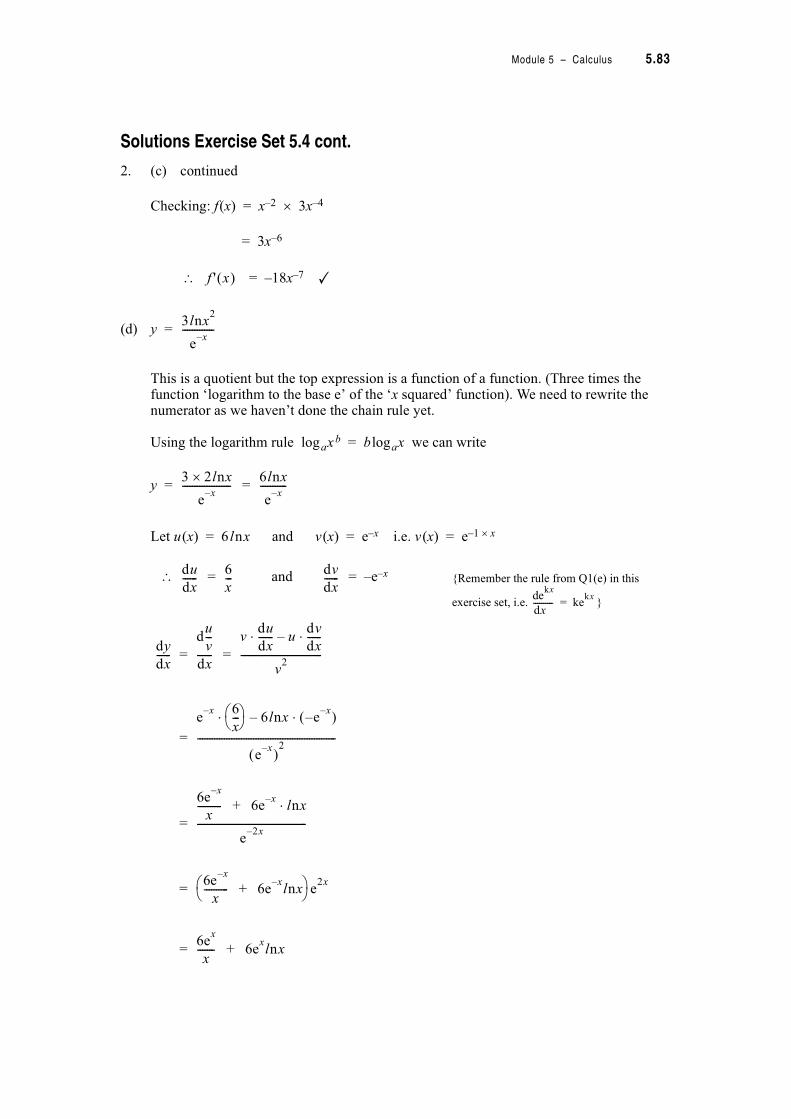
Module 5 – Calculus 5.83
Solutions Exercise Set 5.4 cont.
2. (c) continued
Checking: f(x) = x–2 " 3x–4
= 3x–6
$ = –18x–7 ✓
(d) y =
This is a quotient but the top expression is a function of a function. (Three times the function ‘logarithm to the base e’ of the ‘x squared’ function). We need to rewrite the numerator as we haven’t done the chain rule yet.
Using the logarithm rule logaxb = blogax we can write
y = =
Let u(x) = 6 lnx and v(x) = e–x i.e. v(x) = e–1 " x
$ = and = –e–x {Remember the rule from Q1(e) in this
exercise set, i.e. }
= =
=
=
=
=
f ' x !
3lnx2
ex–
-------------
3 2lnx"
ex–
--------------------6lnx
ex–
-----------
du
dx------
6
x---
dv
dx------
dekx
dx---------- ke
kx=
dy
dx------
du
v---
dx------
vdu
dx------= u
dv
dx------=–
v2
---------------------------------
ex– 6
x---2 3
6 7 6lnx ex–
– !=–=
ex– !
2---------------------------------------------------------
6ex–
x---------- 6e
x–lnx=+
e2x–
---------------------------------------------
6ex–
x---------- 6e
x–lnx+2 3
6 7 e2x
6ex
x------- 6e
xlnx+
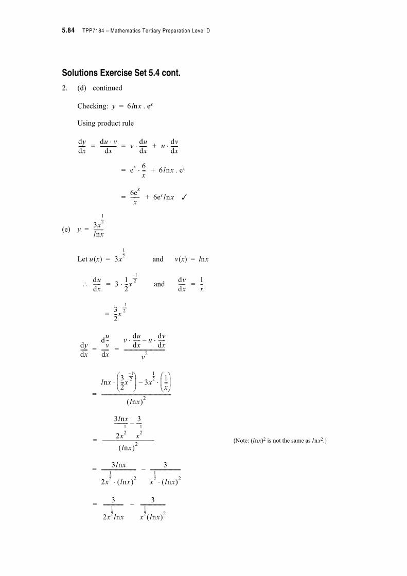
5.84 TPP7184 – Mathematics Tertiary Preparation Level D
Solutions Exercise Set 5.4 cont.
2. (d) continued
Checking: y = 6 lnx . ex
Using product rule
= = +
= + 6 lnx . ex
= + 6ex lnx ✓
(e) y =
Let u(x) = and v(x) = lnx
$ = and =
=
= =
=
= {Note: (lnx)2 is not the same as lnx2.}
= –
= –
dy
dx------
du v=dx
------------- vdu
dx------= u
dv
dx------=
ex 6
x---=
6ex
x-------
3x
1
2---
lnx--------
3x
1
2---
du
dx------ 3
1
2---x
1–
2------
=dv
dx------
1
x---
3
2---x
1–
2------
dy
dx------
du
v---
dx------
vdu
dx------= u
dv
dx------=–
v2
---------------------------------
lnx3
2---x
1–
2------
2 34 56 7
3x
1
2--- 1
x---
2 34 56 7
=–=
lnx !2--------------------------------------------------------
3lnx
2x
1
2---
-----------3
x
1
2---
----–
lnx !2------------------------------------------
3lnx
2x
1
2---
lnx !2=
----------------------------3
x
1
2---
lnx !2=
------------------------
3
2x
1
2---
lnx
----------------3
x
1
2---
lnx !2
--------------------

Module 5 – Calculus 5.85
Solutions Exercise Set 5.4 cont.
2. continued
(f) f(x) =
Let u(x) = sin x and v(x) = cos x
$ = cos x and = –sin x
= =
=
=
= {Using Pythagoras Rule: sin2 # + cos2 # = 1}
= sec2 x
Here you have proved that the derivative of tan x is sec2 x
(g) y =
Let u(x) = cos x and v(x) = sin x
$ = –sin x and = cos x
= =
=
=
=
=
= –cosec2 x
Here you have found that the derivative of cot x is –cosec2 x
xsin
xcos-----------
du
dx------
dv
dx------
f ' x !d
u
v---
dx------
vdu
dx------= u
dv
dx------=–
v2
---------------------------------
xcos xcos ! xsin xsin– !=–=
x2
cos------------------------------------------------------------------------
x2
cos x2
sin+
x2
cos---------------------------------
1
x2
cos-------------
xcos
xsin-----------
du
dx------
dv
dx------
dy
dx------
du
v---
dx------
vdu
dx------= u
dv
dx------=–
v2
---------------------------------
xsin xsin– ! xcos xcos !=–=
x2
sin------------------------------------------------------------------------
x2
sin– x2
cos–
x2
sin-------------------------------------
1– x2
sin x2
cos+ !
x2
sin--------------------------------------------
1–
x2
sin------------
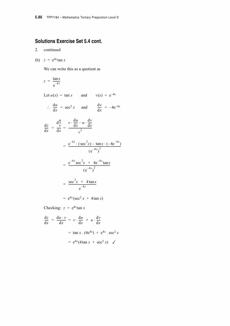
5.86 TPP7184 – Mathematics Tertiary Preparation Level D
Solutions Exercise Set 5.4 cont.
2. continued
(h) z = e4x tan x
We can write this as a quotient as
z =
Let u(x) = tan x and v(x) = e–4x
$ = sec2 x and = –4e–4x
= =
=
=
=
= e4x(sec2 x + 4tan x)
Checking: z = e4x tan x
= = +
= tan x . (4e4x) + e4x . sec2 x
= e4x(4tan x + sec2 x) ✓
xtan
e4x–
----------
du
dx------
dv
dx------
dz
dx------
du
v---
dx------
vdu
dx------= u
dv
dx------=–
v2
---------------------------------
e4x–
x2
sec ! xtan 4e4x–
– !=–=
e4x– !
2--------------------------------------------------------------------------
e4x–
x2
sec 4e4x–
xtan+
e4x– !
2-----------------------------------------------------------
x2
sec 4 xtan+
e4x–
---------------------------------------
dz
dx------
du v=dx
------------- vdu
dx------= u
dv
dx------=

Module 5 – Calculus 5.87
Solutions Exercise Set 5.4 cont.
3. Slope of tangent at x = 1 will equal the derivative of the function at x = 2
f(x) =
Let u = 3x2 and v = 5x2 + 7x
$ = 6x and = 10x + 7
=
=
When x = 2
=
=
=
$ Equation to the tangent is given by
y = x + c
We know the x co-ordinate of one point on the tangent, i.e. x = 2; to find the corresponding y co-ordinate substitute in f(x) for x.
When x = 2
f(x) =
=
=
=
3x2
5x2
7x+--------------------
du
dx------
dv
dx------
du
v---
dx------
vdu
dx------= u
dv
dx------=–
v2
---------------------------------
5x2
7x+ ! 6x 3x2
10x 7+ !=–=
5x2
7x+ !2
------------------------------------------------------------------------------------
du
v---
dx------
5 22
7 2"+" ! 6 2 3 22
10 2 7+" !""–""
5 22
7 2"+" !2
-----------------------------------------------------------------------------------------------------------------------
20 14+ ! 12 12 20 7+ !"–"
20 14+ !2--------------------------------------------------------------------------
21
289---------
21
289---------
3x2
5x2
7x+--------------------
3 22"
5 22
7 2"+"---------------------------------
12
34------
6
17------
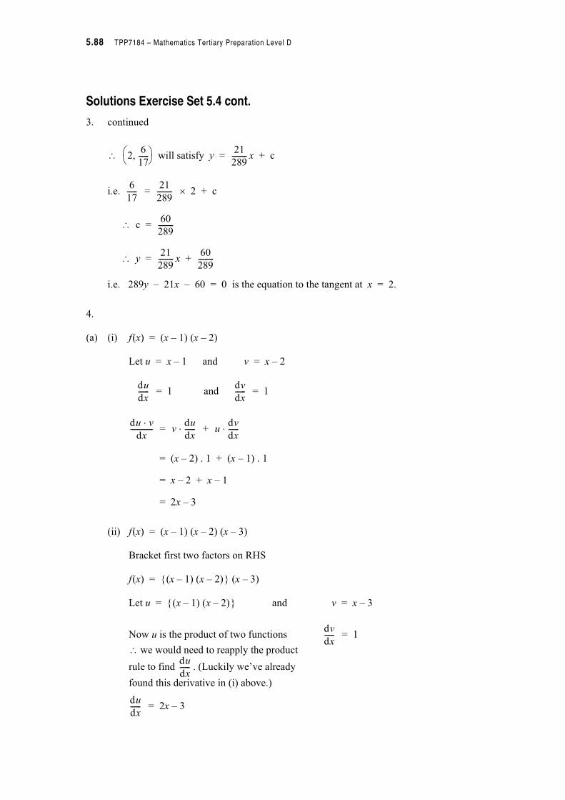
5.88 TPP7184 – Mathematics Tertiary Preparation Level D
Solutions Exercise Set 5.4 cont.
3. continued
$ will satisfy y = x + c
i.e. = " 2 + c
$ c =
$ y = x +
i.e. 289y – 21x – 60 = 0 is the equation to the tangent at x = 2.
4.
(a) (i) f(x) = (x – 1) (x – 2)
Let u = x – 1 and v = x – 2
= 1 and = 1
= +
= (x – 2) . 1 + (x – 1) . 1
= x – 2 + x – 1
= 2x – 3
(ii) f(x) = (x – 1) (x – 2) (x – 3)
Bracket first two factors on RHS
f(x) = {(x – 1) (x – 2)} (x – 3)
Let u = {(x – 1) (x – 2)} and v = x – 3
Now u is the product of two functions = 1
$ we would need to reapply the product
rule to find . (Luckily we’ve already
found this derivative in (i) above.)
= 2x – 3
26
17------<2 3
6 7 21
289---------
6
17------
21
289---------
60
289---------
21
289---------
60
289---------
du
dx------
dv
dx------
du v=dx
------------- vdu
dx------= u
dv
dx------=
dv
dx------
du
dx------
du
dx------

Module 5 – Calculus 5.89
Solutions Exercise Set 5.4 cont.
4. (a) (ii) continued
= +
= (x – 3) . (2x – 3) + {(x – 1) (x – 2)} . 1
= 2x2 – 9x + 9 + x2 – 3x + 2
= 3x2 – 12x + 11
(iii) f(x) = (x – 1) (x – 2) (x – 3) (x – 4)
Bracket first three factors on RHS
f(x) = {(x – 1) (x – 2) (x – 3)} (x – 4)
Let u = {(x – 1) (x – 2) (x – 3)} and v = (x – 4)
= 3x2 – 12x + 11 {from (ii) above} = 1
= +
= (x – 4) (3x2 – 12x + 11) + {(x – 1) (x – 2) (x – 3)} . 1
= 3x3 – 12x2 + 11x – 12x2 + 48x – 44 + {x3 – 6x2 + 11x – 6}
= 4x3 – 30x2 + 70x – 50
(b) If f(x) = (x – r1) (x – r2) (x – r3) (x – r4) … (x – rn–1) (x – rn)
= (x – ri) See Note 1
= (x – rn) {(x – r1) (x – r2) (x – r3) … (x – rn–1)} +
{(x – r1) (x – r2) (x – r3) … (x – rn–1)}
= (x – rn) (x – ri) + (x – ri)
Notes
1. > is the symbol for product in the same way as ? is the symbol for summing.
du v=dx
------------- vdu
dx------= u
dv
dx------=
du
dx------
dv
dx------
du v=dx
------------- vdu
dx------= u
dv
dx------=
i=1
n
>
f ' x ! f '
f '
i=1
n-1
>i=1
n-1
>
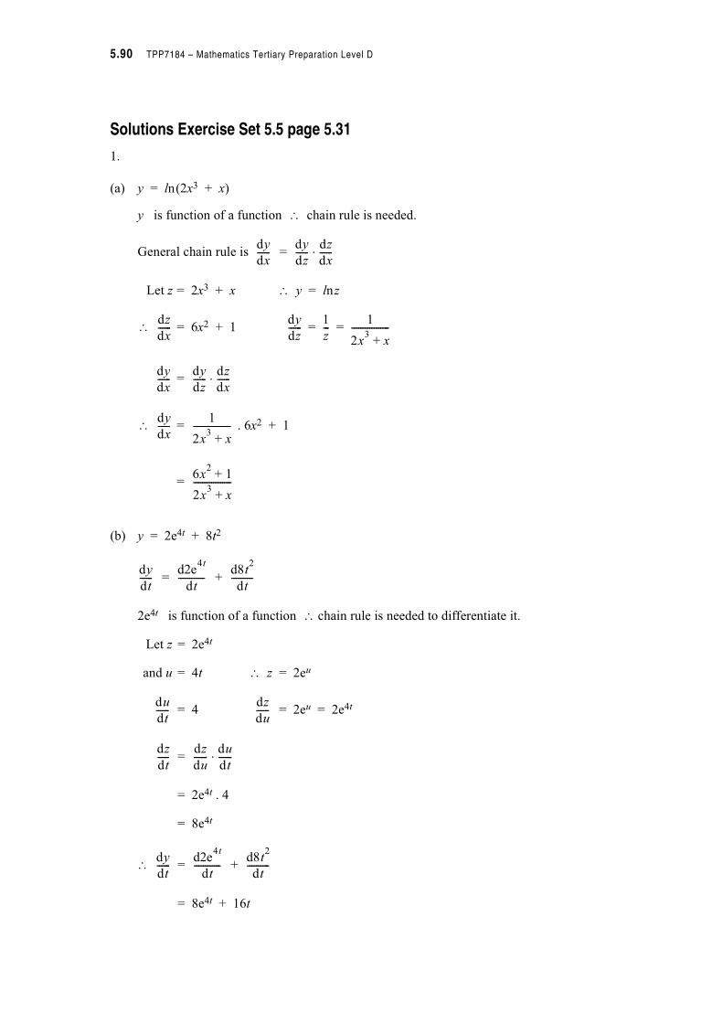
5.90 TPP7184 – Mathematics Tertiary Preparation Level D
Solutions Exercise Set 5.5 page 5.31
1.
(a) y = ln(2x3 + x)
y is function of a function $ chain rule is needed.
General chain rule is =
Let z = 2x3 + x $ y = lnz
$ = 6x2 + 1
=
$ = . 6x2 + 1
=
(b) y = 2e4t + 8t2
= +
2e4t is function of a function $ chain rule is needed to differentiate it.
Let z = 2e4t
and u = 4t $ z = 2eu
= 4 = 2eu = 2e4t
=
= 2e4t . 4
= 8e4t
$ = +
= 8e4t + 16t
dy
dx------
dy
dz------
dz
dx------=
dz
dx------
dy
dz------
1
z---
1
2x3
x+-----------------= =
dy
dx------
dy
dz------
dz
dx------=
dy
dx------
1
2x3
x+-----------------
6x2
1+
2x3
x+-----------------
dy
dt------
d2e4t
dt------------
d8t2
dt----------
du
dt------
dz
du------
dz
dt-----
dz
du------
du
dt------=
dy
dt------
d2e4t
dt------------
d8t2
dt----------

Module 5 – Calculus 5.91
Solutions Exercise Set 5.5 cont.
1. continued
(c) y = sin 4x – cos x2 + tan
Each term on the RHS is function of a function. So the chain rule needs to be used to differentiate each term.
Instead of declaring a lot more variables and applying the chain rule for each term we can shorten the work for each term by multiplying ‘the derivative of the outside function’ by ‘the derivative of the inside function’. [Note: Technically this is not exactly what you are doing.}
= 4cos 4x + sin x2 + sec2
If you have trouble applying the chain rule in your head, do not be concerned — simply declare variables and apply the rule as required for each term. As you use the rule more, you will be able to omit some steps.(d) y = cot2 x
= (cot x)2
= 2
y is a function of a function of a function of x
Let u = tan x and v = = , then y = v2
Then = {simply extending the chain rule}
1
4---
x
2---
‘derivative of outside function’
‘derivative of inside function’
‘derivative of outside function’
‘derivative of inside function’
‘derivative of outside function’
‘derivative of inside function’
= (cos 4x) . (4) – . + . dy
dx------
1
4---x
2sin–
2 34 56 7 x
2---
2 34 56 7 x
2---
2
sec2 34 56 7 1
2---
2 34 56 7
x
2---
1
4---
1
2---
x
2---
1
xtan----------2 3
6 7
1
xtan----------
1
u---
dy
dx------
dy
dv------
dv
du------
du
dx------= =
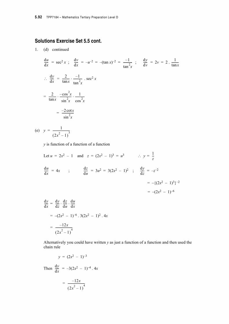
5.92 TPP7184 – Mathematics Tertiary Preparation Level D
Solutions Exercise Set 5.5 cont.
1. (d) continued
= sec2 x ; = –u–2 = –(tan x)–2 = ; = 2v = 2 .
$ = . sec2 x
=
=
(e) y =
y is function of a function of a function
Let u = 2x2 – 1 and z = (2x2 – 1)3 = u3 $ y =
= 4x ; = 3u2 = 3(2x2 – 1)2 ; = –z–2
= –{(2x2 – 1)3}–2
= –(2x2 – 1)–6
=
= –(2x2 – 1)–6 . 3(2x2 – 1)2 . 4x
=
Alternatively you could have written y as just a function of a function and then used the chain rule
y = (2x2 – 1)–3
Then = –3(2x2 – 1)–4 . 4x
=
du
dx------
dv
dx------
1–
x2
tan-------------
dy
dv------
1
xtan----------
dy
dx------
2
xtan----------
1–
x2
tan-------------=
2
xtan----------
x2
cos–
x2
sin-----------------
1
x2
cos-------------= =
2 xcot–
x2
sin-----------------
1
2x2
1– !3
------------------------
1
z---
du
dx------
dz
du------
dy
dz------
dy
dx------
dy
dz------
dz
du------
du
dx------= =
12x–
2x2
1– !4
------------------------
dy
dx------
12x–
2x2
1– !4
------------------------
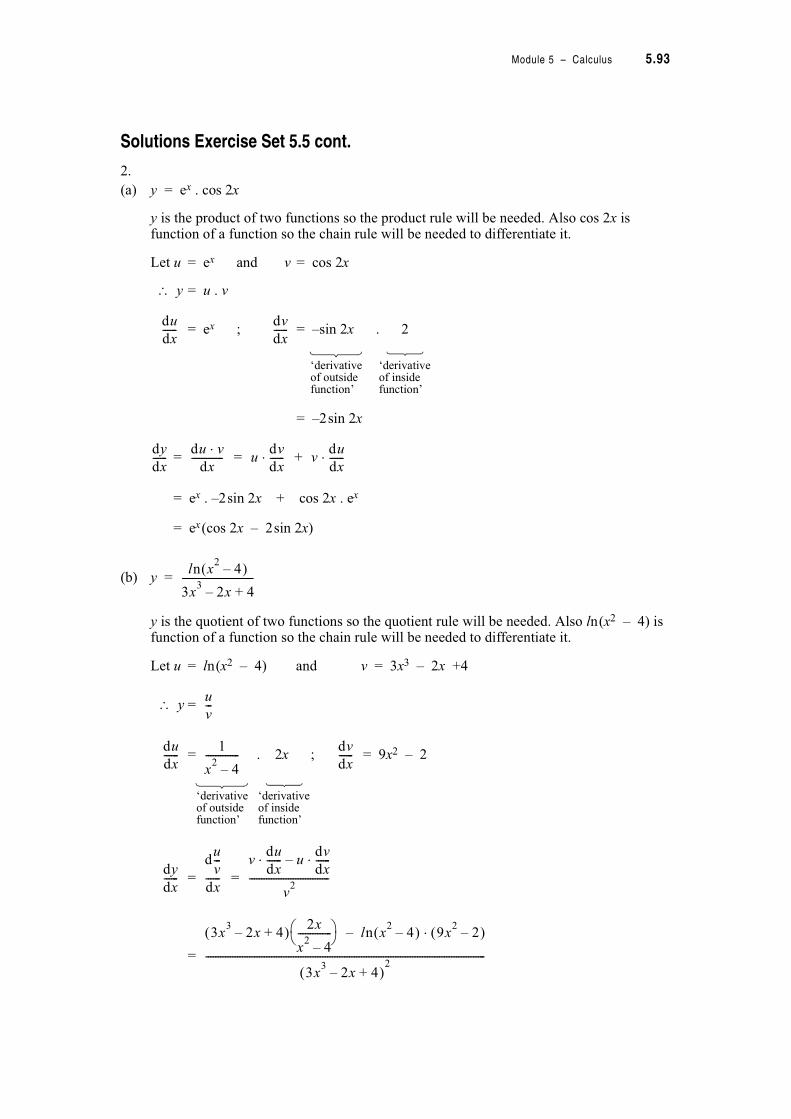
Module 5 – Calculus 5.93
Solutions Exercise Set 5.5 cont.
2.
(a) y = ex . cos 2x
y is the product of two functions so the product rule will be needed. Also cos 2x is function of a function so the chain rule will be needed to differentiate it.
Let u = ex and v = cos 2x
$ y = u . v
= ex ; = –sin 2x . 2
= –2sin 2x
= = +
= ex . –2sin 2x + cos 2x . ex
= ex(cos 2x – 2sin 2x)
(b) y =
y is the quotient of two functions so the quotient rule will be needed. Also ln(x2 – 4) is function of a function so the chain rule will be needed to differentiate it.
Let u = ln(x2 – 4) and v = 3x3 – 2x +4
$ y =
= . 2x ; = 9x2 – 2
= =
=
du
dx------
dv
dx------
‘derivative of outside function’
‘derivative of inside function’
dy
dx------
du v=dx
------------- udv
dx------= v
du
dx------=
ln x2
4– !
3x3
2x 4+–-----------------------------
u
v---
du
dx------
1
x2
4–--------------
dv
dx------
‘derivative of outside function’
‘derivative of inside function’
dy
dx------
du
v---
dx------
vdu
dx------= u
dv
dx------=–
v2
---------------------------------
3x3
2x– 4+ !2x
x2
4–--------------2 3
6 7 ln x2
4– ! 9x2
2– !=–
3x3
2x– 4+ !2
-------------------------------------------------------------------------------------------------------------------
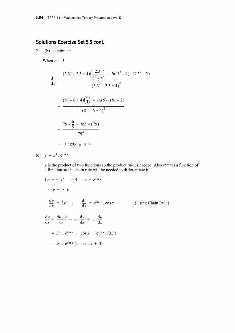
5.94 TPP7184 – Mathematics Tertiary Preparation Level D
Solutions Exercise Set 5.5 cont.
2. (b) continued
When x = 3
=
=
=
= –5.1828 " 10–3
(c) y = x3 . esin x
y is the product of two functions so the product rule is needed. Also esin x is a function of a function so the chain rule will be needed to differentiate it.
Let u = x3 and v = esin x
$ y = u . v
= 3x2 ; = esin x . cos x {Using Chain Rule}
= = +
= x3 . esin x . cos x + esin x . (3x2)
= x2 . esin x (x . cos x + 3)
dy
dx------
3.33
2.3– 4+ !2.3
32
4–--------------2 3
6 7 ln 32
4– ! 9.32
2– !=–
3.33
2.3– 4+ !2
------------------------------------------------------------------------------------------------------------------------
81 6– 4+ !6
5---2 3
6 7 ln 5 ! 81 2– !=–
81 6– 4+ !2-------------------------------------------------------------------------------------
796
5--- ln5 79 !"–"
792
-------------------------------------------------
du
dx------
dv
dx------
dy
dx------
du v=dx
------------- udv
dx------= v
du
dx------=
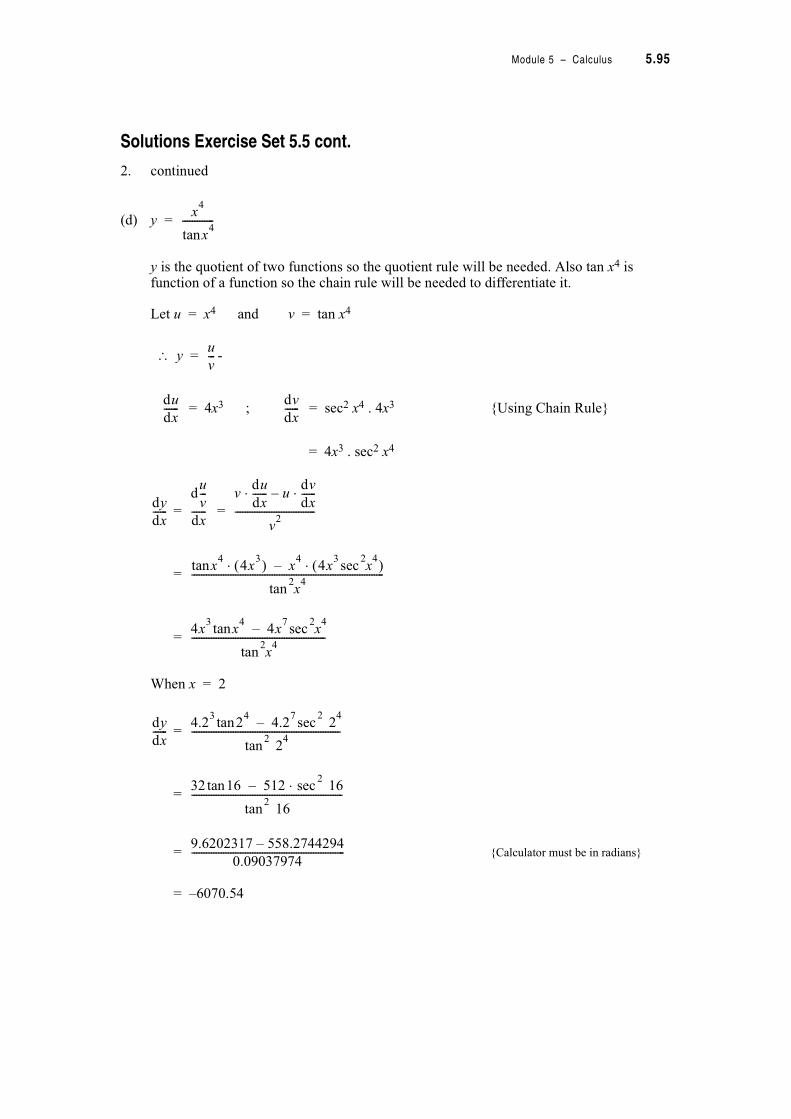
Module 5 – Calculus 5.95
Solutions Exercise Set 5.5 cont.
2. continued
(d) y =
y is the quotient of two functions so the quotient rule will be needed. Also tan x4 is function of a function so the chain rule will be needed to differentiate it.
Let u = x4 and v = tan x4
$ y = -
= 4x3 ; = sec2 x4 . 4x3 {Using Chain Rule}
= 4x3 . sec2 x4
= =
=
=
When x = 2
=
=
= {Calculator must be in radians}
= –6070.54
x4
x4
tan-------------
u
v---
du
dx------
dv
dx------
dy
dx------
du
v---
dx------
vdu
dx------= u
dv
dx------=–
v2
---------------------------------
x4
tan 4x3 ! x
44x
3x
2 4sec !=–=
x2 4
tan-------------------------------------------------------------------------------
4x3
x4
tan 4x7
x2 4
sec–
x2 4
tan-------------------------------------------------------
dy
dx------
4.23
24
tan 4.27
22 4
sec–
22 4
tan-------------------------------------------------------------
32 16tan 512 162
sec=–
162
tan--------------------------------------------------------------
9.6202317 558.2744294–
0.09037974---------------------------------------------------------------
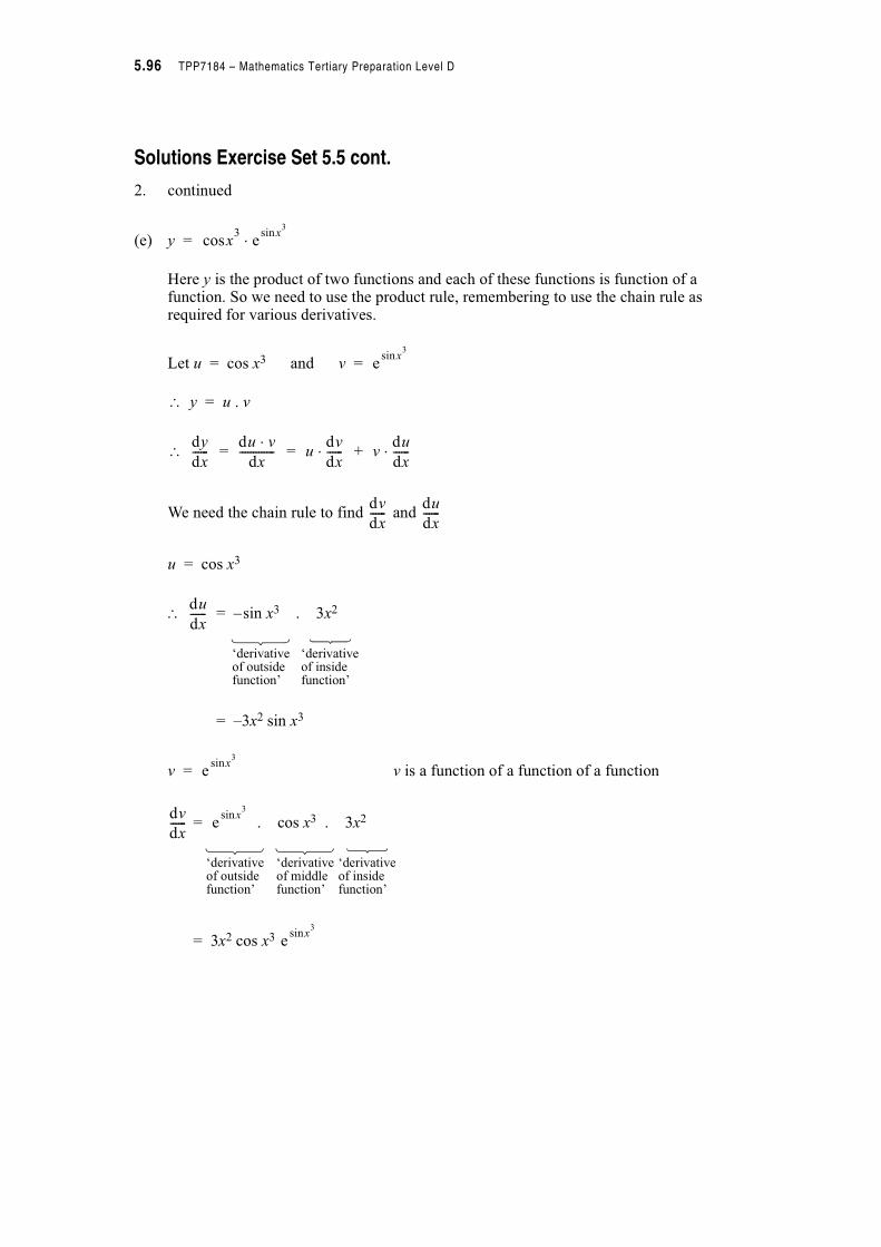
5.96 TPP7184 – Mathematics Tertiary Preparation Level D
Solutions Exercise Set 5.5 cont.
2. continued
(e) y =
Here y is the product of two functions and each of these functions is function of a function. So we need to use the product rule, remembering to use the chain rule as required for various derivatives.
Let u = cos x3 and v =
$ y = u . v
$ = = +
We need the chain rule to find and
u = cos x3
$ = –sin x3 . 3x2
= –3x2 sin x3
v = v is a function of a function of a function
= . cos x3 . 3x2
= 3x2 cos x3
x3
cos ex
3sin=
ex
3sin
dy
dx------
du v=dx
------------- udv
dx------= v
du
dx------=
dv
dx------
du
dx------
du
dx------
‘derivative of outside function’
‘derivative of inside function’
ex
3sin
dv
dx------ e
x3
sin
‘derivative of outside function’
‘derivative of inside function’
‘derivative of middle function’
ex
3sin

Module 5 – Calculus 5.97
Solutions Exercise Set 5.5 cont.
2. (e) continued
= = +
= cos x3 . 3x2 cos x3 + . –3x2 sin x3
= 3x2 cos2 x3 – 3x2 sin x3
= 3x2 (cos2 x3 – sin x3)
When x =
=
=
= 0.424792476(0.98445621 – 0.124674733)
= 0.3652
3.
(a) Assume x is a function of t, then
=
Given = 2 + 3cos x and = 2sin x
To find we find the reciprocal of
$ = {This is a useful technique to remember}
$ = . (2 + 3cos x)
=
= +
= cosec x + cot x
dy
dx------
du v=dx
------------- udv
dx------= v
du
dx------=
ex
3sin
ex
3sin
ex
3sin
ex
3sin
ex
3sin
1
2---
dy
dx------ 3
1
2---2 3
6 72
e
1
2---2 3
6 73
sin1
2---2 3
6 72 3
cos1
2---2 3
6 73
sin–2 36 7
3
8---e
1
8---sin
2 1
8---cos
1
8---sin–2 3
6 7
dx
dt------
dx
dv------
dv
dt------=
dv
dt------
dv
dx------
dx
dv------
dv
dx------
dx
dv------
1
2 xsin-------------
dx
dt------
1
2 xsin-------------
2 3 xcos+
2 xsin------------------------
2
2 xsin-------------
3 xcos
2 xsin--------------
3
2---
5.98 TPP7184 – Mathematics Tertiary Preparation Level D
Solutions Exercise Set 5.5 cont.
3. continued
(b) Assume x is a function of t, then
=
Given = lnx and =
$ = x {Finding the reciprocal}
$ = lnx . x
= xlnx
(c) Assume z is a function of t, then
Given = e–2t and = 4e2t
$ =
$ =
=
=
When t = 0.25
=
=
= 0.092
dx
dt------
dz
dt-----
dx
dz------=
dz
dt-----
dz
dx------
1
x---
dx
dz------
dx
dt------
dz
dt-----
dp
dt------=
dz
dp------=
dp
dt------
dp
dz------
dz
dp------
1
4e2t
---------
dz
dt----- e
2 t– 1
4e2 t
---------=
e2t–
e2t–=
4----------------------
e4t–
4--------
dz
dt-----
e4– 0.25"
4-------------------
e1–
4-------
Module 5 – Calculus 5.99
Solutions Exercise Set 5.5 cont.
4.
(a) N = Cekt
We require the rate . The chain rule will be needed.
Let u = kt $ N = Ceu
$ = k and $ = Ceu = Cekt
$ = .
= Cekt . k
= Ckekt {You could have simply used the rule }
When t = 6 seconds
= C " k " ek " 6
= Cke6k bacteria per second.
$ After 6 seconds the rate of increase of the population is Cke6k bacteria per second.
(b)
Given x0 = 250 kg
$
We require the rate . The chain rule will be needed
=
=
=
dN
dt-------
du
dt------
dN
du-------
dN
dt-------
dN
du-------
du
dt------
dckx
dx----------- ke
kx=
dN
dt-------
x x0e
1
2---– t
=
x 250e
1
2---– t
=
dx
dt------
dx
dt------
dx
du------
du
dt------=
dx
dt------ 250e
1
2---– t 1
2---–=
125– e
1
2---– t
5.100 TPP7184 – Mathematics Tertiary Preparation Level D
Solutions Exercise Set 5.5 cont.
4. (b) continued
When t = 10 years
=
= –125 " 0.006738
= –0.842 kg per year {Note negative sign shows the decay}
$ After 10 years the initial amount of 250 kg is decaying at the rate of 0.842 kg per year.
(c) (i) T – Ta = (To – Ta)e–0.05596t See Note 1
Given Ta = 20@C and To = 90@C
$ T – 20 = (90 – 20)e–0.05596t
$ T = 20 + 70e–0.05596t
The chain rule is needed to find
$ = 70 e–0.05596t " (–0.05596)
= –3.9172e–0.05596t {Note Negative sign shows cooling}
i.e. the rate of cooling is 3.9172e–0.05596t degrees Centigrade per second.
Notes
1. This is an application of Newton’s Law of Cooling.
dx
dt------ 125– e
1
2--- 10"–
dT
dt------
dT
dt------

Module 5 – Calculus 5.101
Solutions Exercise Set 5.5 cont.
5.
(a) Rate required is
Given = 0.4 cm2 s–1
Relationship between A and r is A = ;r2
$ = 2;r
=
= 0.4 "
= cm s–1
i.e. the rate of increase in the radius when the area is increasing at 0.4 cm2 s–1 is
cm s–1.
(b) Rate required is
Given = 0.5 cm2 s–1
Relationship between A and l is A = l2
$ = 2l
r cm
dr
dt-----
dA
dt-------
dA
dr-------
{ To make sure you have the correct formula you can imagine cancelling dA on the RHSto give = }{You need the reciprocal of
= 2 r ! = }
dr
dt-----
dr
dt-----
dA
dr-------
dA
dr-------
dr
dA-------
1
2 r---------
dr
dt-----
dA
dt-------
dr
dA-------"
1
2 r---------
0.2
r-------
0.2
r-------
dl
dt-----
l cm
l cm
dA
dt-------
dA
dl-------

5.102 TPP7184 – Mathematics Tertiary Preparation Level D
Solutions Exercise Set 5.5 cont.
5. (b) continued
= .
= 0.5 #
= cm s–1
i.e. the rate of increase of the length of the side when the area is increasing at
0.5 cm2 s–1 is cm s–1.
6.
(a) Rate required is
We are not given another rate but we know that both V and S are functions of the radius, r. So we’ll be able to
get by using a chain rule involving and .
V = r2 # h
= r2 # 7
! = 14 r
S = 2 r2 + 2 rh
= 2 r2 + 14 r
! = 4 r + 14
{ To make sure you have the correct formula you can imagine dA cancelling on the RHSto give = }{ is the reciprocal of }
dl
dt-----
dl
dt-----
dl
dA-------
dA
dl-------
dl
dt-----
dA
dt-------
dl
dA-------
1
2l-----
0.25
l----------
0.25
l----------
7 m
r cm
dV
dS-------
dV
dS-------
dV
dr-------
dS
dr------
dV
dr-------
dS
dr------
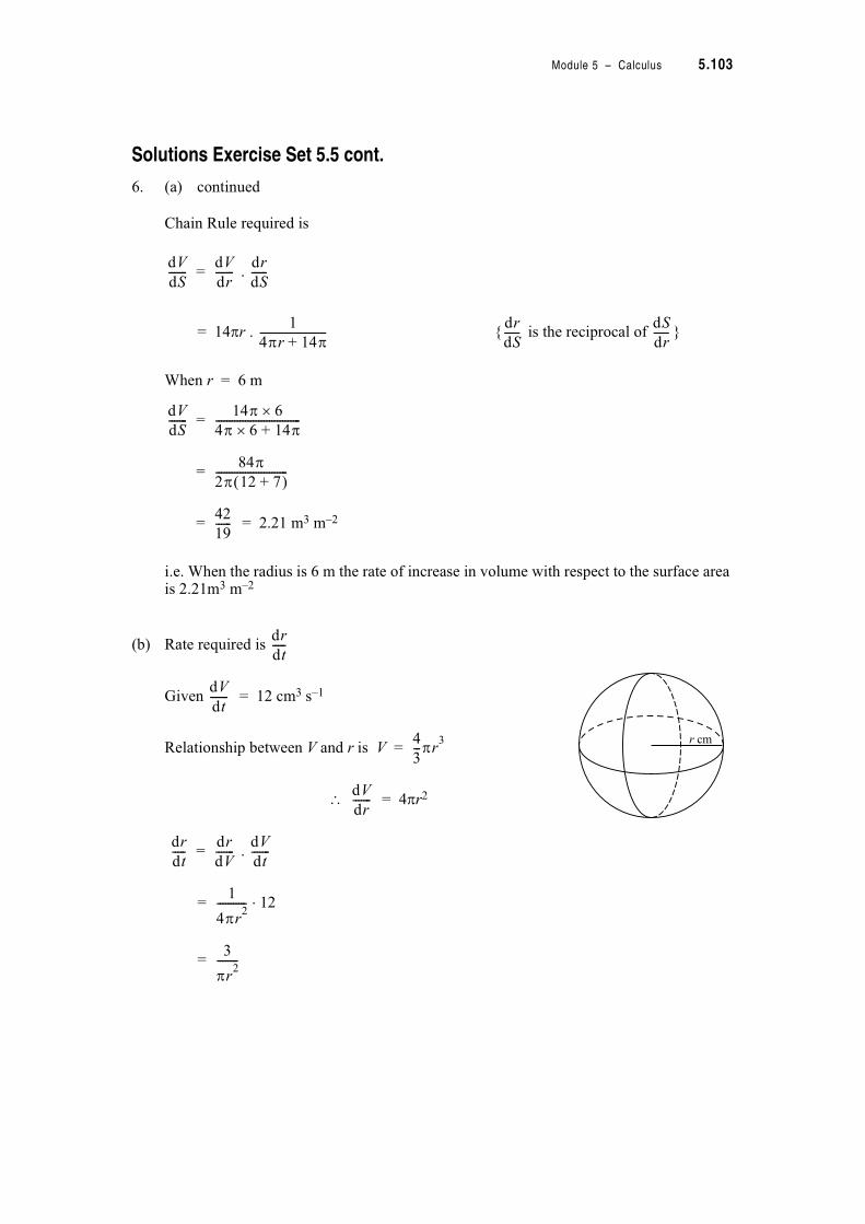
Module 5 – Calculus 5.103
Solutions Exercise Set 5.5 cont.
6. (a) continued
Chain Rule required is
= .
= 14 r . { is the reciprocal of }
When r = 6 m
=
=
= = 2.21 m3 m–2
i.e. When the radius is 6 m the rate of increase in volume with respect to the surface area is 2.21m3 m–2
(b) Rate required is
Given = 12 cm3 s–1
Relationship between V and r is V =
! = 4 r2
= .
=
=
dV
dS-------
dV
dr-------
dr
dS------
1
4 r 14 +-------------------------
dr
dS------
dS
dr------
dV
dS-------
14 6#4 6 14 +#--------------------------------
84 2 12 7+$ %---------------------------
42
19------
r cm
dr
dt-----
dV
dt-------
4
3--- r
3
dV
dr-------
dr
dt-----
dr
dV-------
dV
dt-------
1
4 r2
----------- 12"
3
r2
--------
5.104 TPP7184 – Mathematics Tertiary Preparation Level D
Solutions Exercise Set 5.5 cont.
6. (b) continued
We need to find when V = cm3
i.e. when =
! r3 = #
=
! r = cm
! =
= cm s–1
i.e. When the volume is cm3 the volume is increasing at 12 cm3 s–1, and the radius is
increasing at cm s–1.
dr
dt-----
9 2
------
9 2
------4
3--- r
3
9 2
------3
4 ------
27
8------
3
2---
dr
dt-----
3
3
2---& '( )
2--------------
4
3 ------
9 2
------4
3 ------
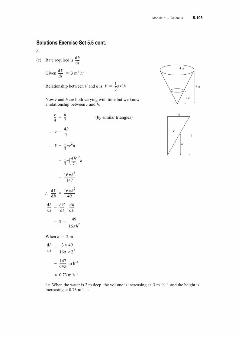
Module 5 – Calculus 5.105
Solutions Exercise Set 5.5 cont.
6.
(c) Rate required is
Given = 3 m3 h–1
Relationship between V and h is V =
Now r and h are both varying with time but we knowa relationship between r and h.
= {by similar triangles}
! r =
! V =
=
=
! =
= .
= 3 #
When h = 2 m
=
= m h–1
* 0.73 m h–1
i.e. When the water is 2 m deep, the volume is increasing at 3 m3 h–1 and the height is increasing at 0.73 m h–1.
2 m
7 m
4 m
4
7
h
r
dh
dt------
dV
dt-------
1
3--- r
2h
r
4---
h
7---
4h
7------
1
3--- r
2h
1
3---
4h
7------& '( )
2
h
16 h3
147---------------
dV
dh-------
16 h2
49---------------
dh
dt------
dV
dt-------
dh
dV-------
49
16 h2
---------------
dh
dt------
3 49#
16 22#
---------------------
147
64 ---------
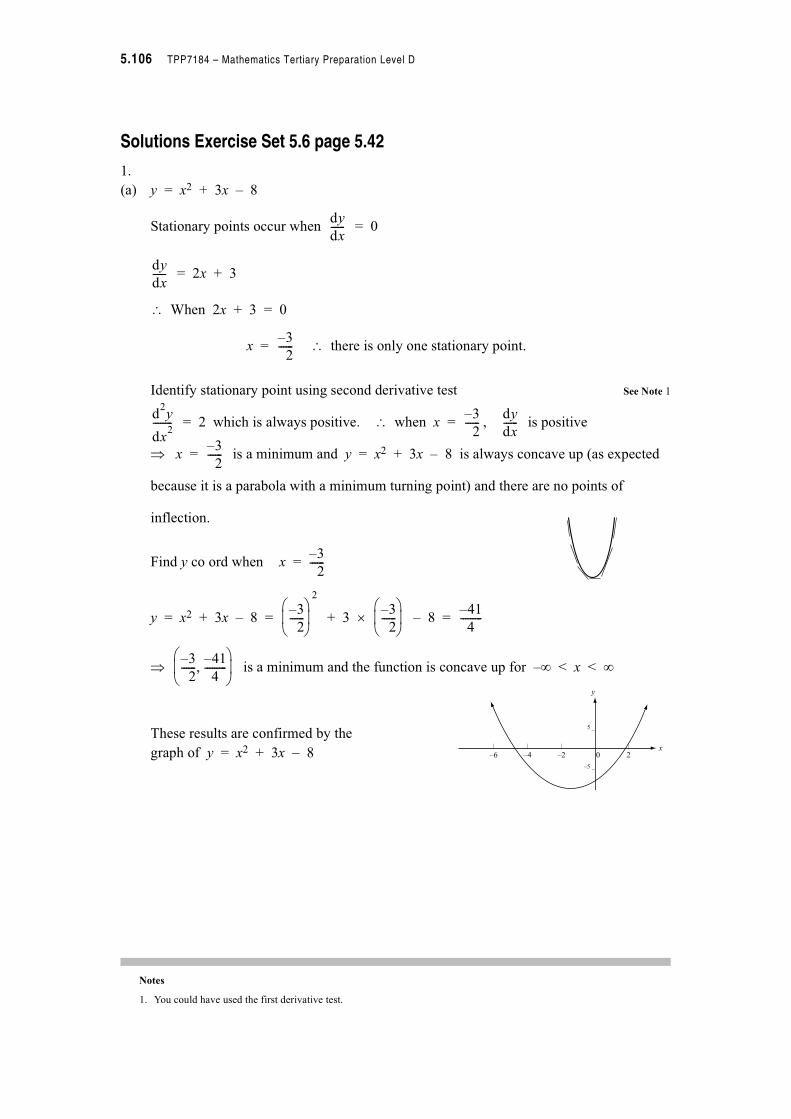
5.106 TPP7184 – Mathematics Tertiary Preparation Level D
Solutions Exercise Set 5.6 page 5.42
1.
(a) y = x2 + 3x – 8
Stationary points occur when = 0
= 2x + 3
! When 2x + 3 = 0
x = ! there is only one stationary point.
Identify stationary point using second derivative test See Note 1
= 2 which is always positive. ! when x = , is positive
+ x = is a minimum and y = x2 + 3x – 8 is always concave up (as expected
because it is a parabola with a minimum turning point) and there are no points of
inflection.
Find y co ord when
y = x2 + 3x – 8 = + 3 # – 8 =
+ is a minimum and the function is concave up for –, < x < ,
These results are confirmed by the
graph of y = x2 + 3x – 8
Notes
1. You could have used the first derivative test.
dy
dx------
dy
dx------
3–
2------
d2y
dx2
--------3–
2------
dy
dx------
3–
2------
x3–
2------=
3–
2------& '- .( )
2
3–
2------& '- .( ) 41–
4---------
3–
2------
41–
4---------/
& '- .( )
| | | |
–6 –4 –2 0 2
5 _
–5 _
x
y

Module 5 – Calculus 5.107
Solutions Exercise Set 5.6 cont.
1. continued
(b) f(x) = x3+ 6x2 – 15x + 8
Stationary points occur where = 0
= 3x2 + 12x – 15
! When 3x2 + 12x – 15 = 0
x2 + 4x – 5 = 0
! (x + 5) (x – 1) = 0
! x = –5 and x = 1 are stationary points.
Identify stationary points using second derivative test.
= 6x + 12
When x = –5, = 6x + 12 = 6 # –5 + 12 which is –ve
! x = –5 is a local maximum
Find y co ord.
When x = –5, f(x) = x3+ 6x2 – 15x + 8
= (–5)3 + 6 # (–5)2 –15 # (–5) + 8 = 108 + (–5,108)
When x = 1, = 6x + 12 = 6 # 1 + 12 which is +ve
! x = 1 is a local minimum
Find y co ord.
When x = 1, f(x) = 13 + 6 # 12 – 15 # 1 + 8 = 0 + (1,0)
We expect to find a point of inflection between the local maximum and adjacent local minimum.
df
dx------
df
dx------
d2f
dx2
--------
d2f
dx2
--------
d2f
dx2
--------
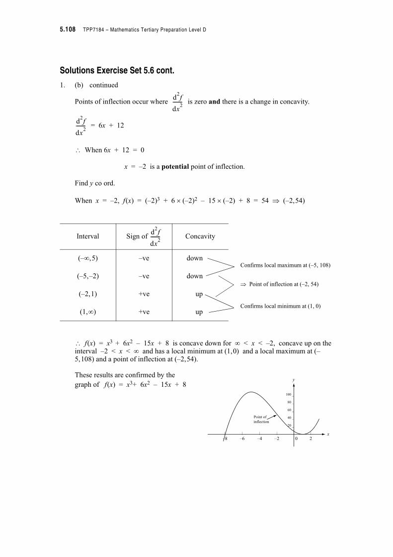
5.108 TPP7184 – Mathematics Tertiary Preparation Level D
Solutions Exercise Set 5.6 cont.
1. (b) continued
Points of inflection occur where is zero and there is a change in concavity.
= 6x + 12
! When 6x + 12 = 0
x = –2 is a potential point of inflection.
Find y co ord.
When x = –2, f(x) = (–2)3 + 6 # (–2)2 – 15 # (–2) + 8 = 54 + (–2,54)
! f(x) = x3 + 6x2 – 15x + 8 is concave down for , < x < –2, concave up on the interval –2 < x < , and has a local minimum at (1,0) and a local maximum at (–5,108) and a point of inflection at (–2,54).
These results are confirmed by the
graph of f(x) = x3+ 6x2 – 15x + 8
d2f
dx2
--------
d2f
dx2
--------
Interval Sign of Concavity
(–,,5) –ve down
(–5,–2) –ve down
(–2,1) +ve up
(1,,) +ve up
d2f
dx2
--------
Confirms local maximum at (–5, 108)
Confirms local minimum at (1, 0)
+ Point of inflection at (–2, 54)
| | | | |
–8 –6 –4 –2 0 2
100 _
80 _
60 _
40 _
20 _
x
y
Point of
inflection
Module 5 – Calculus 5.109
Solutions Exercise Set 5.6 cont.
1.
(c) f(x) = x4 – 4x3 + 6
Stationary points occur where = 0
= 4x3 – 12x2
! When 4x3 – 12x2 = 0
x2(4x – 12) = 0
! x = 0 or 4x – 12 = 0
i.e. x = 0 or x = 3
Identify stationary points using second derivative test.
= 12x2 – 24x
Check x = 3
When x = 3, = 12x2 – 24x = 12 # 32 – 24 # 3 which is +ve
! x = 3 is a local minimum
Find y co ord.
When x = 3, f(x) = x4 – 4x3 + 6 = 34 – 4 # 33 + 6 = –21 + (3,–21)
Check x = 0
When x = 0, = 12x2 – 24x = 12 # 02 – 24 # 0 = 0
! no conclusion can be drawn about the type of stationary point at x = 0 (i.e. the second derivative test has failed). Try first derivative test
• to the near left of x = 0, say at x = –1,
= 4x3 – 12x2 = 4 # (–1)3 – 12 # (–1)2 which is –ve
• to the near right of x = 0, say at x = 1
= 4x3 – 12x2 = 4 # 13 – 12 # 12 which is –ve
! as there has NOT been a change in the sign of the slope across x = 0, there is no maximum or minimum at x = 0 but there may be a point of inflection.
f ' x$ %
f ' x$ %
f '' x$ %
f '' x$ %
f '' x$ %
f ' x$ %
f ' x$ %
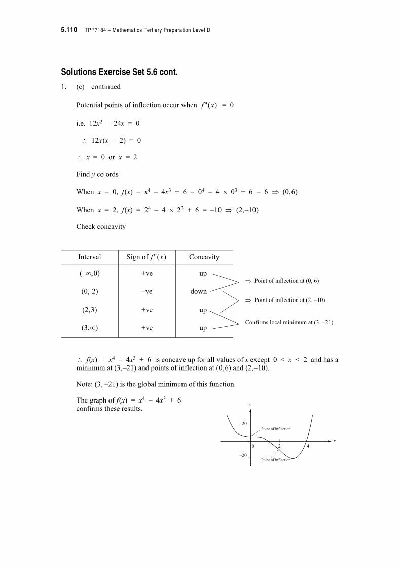
5.110 TPP7184 – Mathematics Tertiary Preparation Level D
Solutions Exercise Set 5.6 cont.
1. (c) continued
Potential points of inflection occur when = 0
i.e. 12x2 – 24x = 0
! 12x(x – 2) = 0
! x = 0 or x = 2
Find y co ords
When x = 0, f(x) = x4 – 4x3 + 6 = 04 – 4 # 03 + 6 = 6 + (0,6)
When x = 2, f(x) = 24 – 4 # 23 + 6 = –10 + (2,–10)
Check concavity
! f(x) = x4 – 4x3 + 6 is concave up for all values of x except 0 < x < 2 and has a minimum at (3,–21) and points of inflection at (0,6) and (2,–10).
Note: (3, –21) is the global minimum of this function.
The graph of f(x) = x4 – 4x3 + 6confirms these results.
f '' x$ %
Interval Sign of Concavity
(–,,0) +ve up
(0, 2) –ve down
(2,3) +ve up
(3,,) +ve up
f '' x$ %
+ Point of inflection at (0, 6)
Confirms local minimum at (3, –21)
+ Point of inflection at (2, –10)
| |
0 2 4
20 _
–20 _
x
y
Point of inflection
Point of inflection
Module 5 – Calculus 5.111
Solutions Exercise Set 5.6 cont.
1. continued
(d) f(x) = x +
Note: f(x) is not defined at x = 0. (It has a vertical asymptote at x = 0)
Stationary points occur where = 0
=
! When = 0
= 0
! x2 – 1 = 0 {provided x 0 0}
! x = +1 or x = –1
Identify stationary points
= 2x–3
When x = 1, is +ve ! x = 1 is a local minimum
Find y co ord. When x = 1, f(x) = x + = 1 + = 2 + (1,2)
When x = –1, is –ve ! x = –1 is a local maximum
Find y co ord. When x = –1, f(x) = –1 + = –2 + (–1,–2)
Potential points of inflection occur when = 0
i.e. 2x–3 = 0 which has no solution because we know when x = 0 the function is not defined.
Check concavity
1
x---
f ' x$ %
f ' x$ % 11
x2
-----–
11
x2
-----–
x2
1–
x2
--------------
f '' x$ %
f '' x$ %
1
x---
1
1---
f '' x$ %
1
1–------
f '' x$ %

5.112 TPP7184 – Mathematics Tertiary Preparation Level D
Solutions Exercise Set 5.6 cont.
1. (d) continued
! f(x) = x + is concave down for –, < x < 0 and concave up for 0 < x < ,
and has a local maximum at (–1,–2) and a local minimum at (1, 2). There are no points of inflection.
The graph of f(x) = x +confirms these results.
2. If when learning is starting to decrease is of interest we need to find the first local
maximum on the interval 0 1 t 1 12 as it is after this maximum that the slope of the
function is negative.
P = 12t2 – t3
= 24t – 3t2
Stationary points occur when = 0
i.e. 24t – 3t2 = 0
! 3t(8 – t) = 0
! t = 0 or (8 – t) = 0
i.e. t = 0 or t = 8
Interval Sign of Concavity
(–,,–1) –ve down
(–1, 0) –ve down
(0,1) +ve up
(1,,) +ve up
f '' x$ %
Confirms local maximum at (–1, –2)
Confirms local minimum at (1, 2)
Care needed here because f(x) is not defined at x = 0
1
x---
| | |
–4 –2 0 2
5 _
5 _
x
y
1
x---
dP
dt-------
dP
dt-------
Module 5 – Calculus 5.113
Solutions Exercise Set 5.6 cont.
2. continued
Now when t = 0, this is obviously the global minimum as learning has not commenced.
When t = 8 is the stationary point of interest. To determine if it is a local maximum we can use the second derivative test.
= 24 – 6t
When t = 8,
= 24 – 6 # 8 which is –ve + local maximum at t = 8 weeks
! The psychologist would conclude that after 8 weeks of study the learning has started to decrease.
3. s = –4.9t2 + 39.2t
(i) Velocity V(t) =
! V(t) = –9.8t + 39.2 m s–1
Checking that this formula is correct for the initial velocity given.
When t = 0, V(t) = –9.8 # 0 + 39.2 = 39.2 m s–1 ✓
(ii) The object reaches its highest point when the velocity is zero.
i.e. 0 = –9.8t + 39.2
! t = 4 s
(iii) Maximum height occurs when V = 0 i.e. when t = 4
s = –4.9t2 + 39.2t
= –4.9 # 42 + 39.2 # 4
= 78.4 m
d2P
dt2
---------
d2P
dt2
---------
ds
dt-----
5.114 TPP7184 – Mathematics Tertiary Preparation Level D
Solutions Exercise Set 5.6 cont.
3. continued
(iv) Acceleration, a(t) =
! a(t) = –9.8 m s–2
(v) The object is in the air for the time it takes for s to start at zero and finish at zero.
! We solve
s = –4.9t2 + 39.2t for s = 0
i.e. 0 = –4.9t2 + 39.2t
! 4.9t(–t + 8) = 0
! t = 0 or t = 8
! the object is in the air 8 seconds.
(vi) We need to find V when t = 8
V = 9.8t + 39.2
! When t = 8, V = –9.8 # 8 + 39.2
= –39.2 m s–1
Note the negative sign on the velocity. Velocity has magnitude and direction. The negative sign indicates that the object is falling back to earth.
dV
dt-------
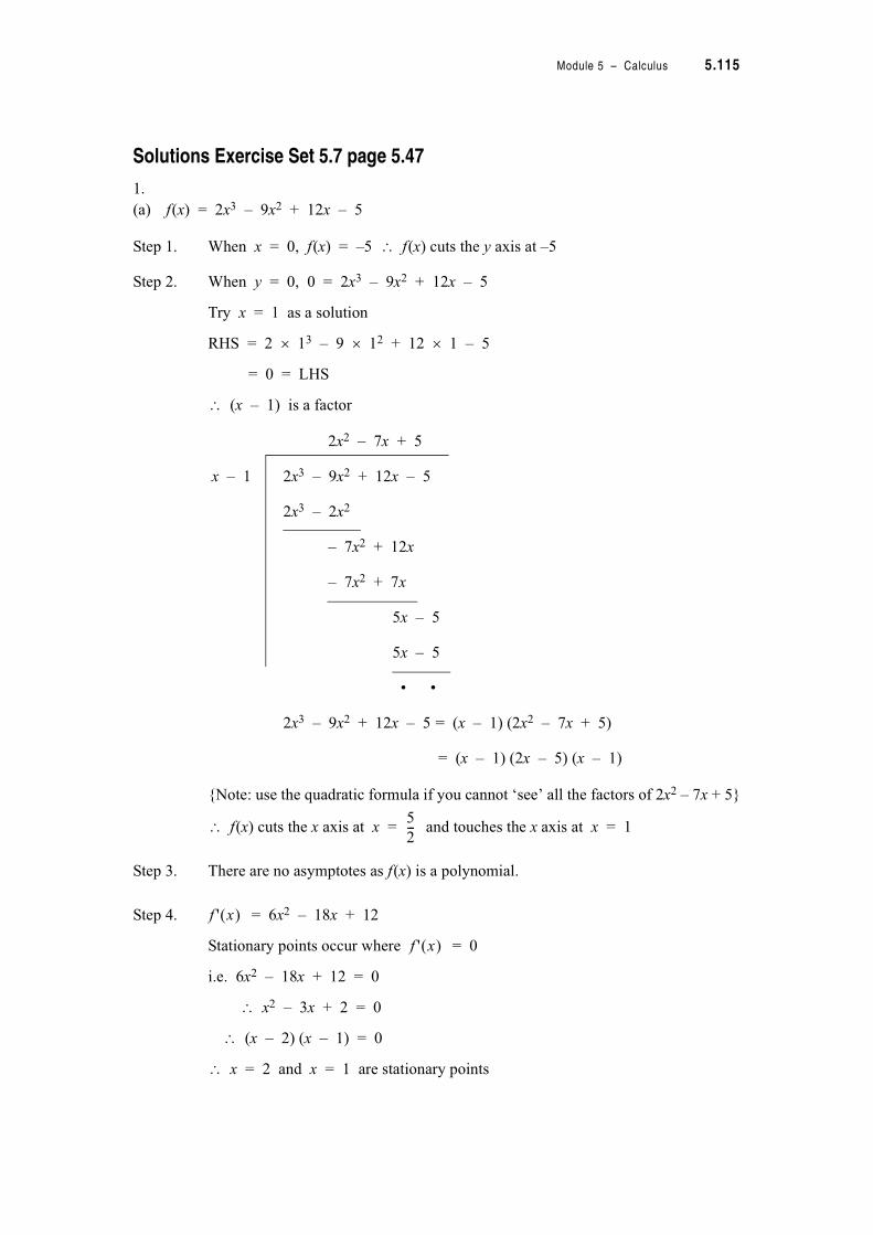
Module 5 – Calculus 5.115
Solutions Exercise Set 5.7 page 5.47
1.
(a) f(x) = 2x3 – 9x2 + 12x – 5
Step 1. When x = 0, f(x) = –5 ! f(x) cuts the y axis at –5
Step 2. When y = 0, 0 = 2x3 – 9x2 + 12x – 5
Try x = 1 as a solution
RHS = 2 # 13 – 9 # 12 + 12 # 1 – 5
= 0 = LHS
! (x – 1) is a factor
{Note: use the quadratic formula if you cannot ‘see’ all the factors of 2x2 – 7x + 5}
! f(x) cuts the x axis at x = and touches the x axis at x = 1
Step 3. There are no asymptotes as f(x) is a polynomial.
Step 4. = 6x2 – 18x + 12
Stationary points occur where = 0
i.e. 6x2 – 18x + 12 = 0
! x2 – 3x + 2 = 0
! (x – 2) (x – 1) = 0
! x = 2 and x = 1 are stationary points
2x2 – 7x + 5
x – 1 2x3 – 9x2 + 12x – 5
2x3 – 2x2
– 7x2 + 12x
– 7x2 + 7x
5x – 5
5x – 5
• •
2x3 – 9x2 + 12x – 5 = (x – 1) (2x2 – 7x + 5)
= (x – 1) (2x – 5) (x – 1)
5
2---
f ' x$ %
f ' x$ %
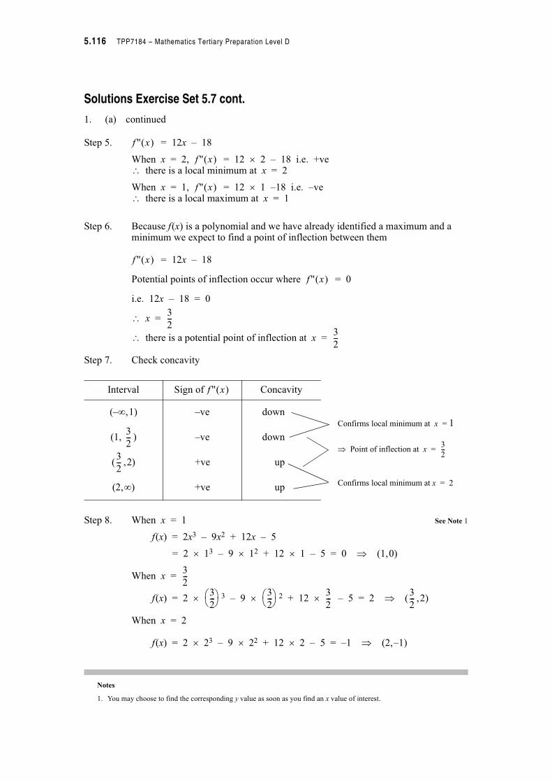
5.116 TPP7184 – Mathematics Tertiary Preparation Level D
Solutions Exercise Set 5.7 cont.
1. (a) continued
Step 5. = 12x – 18
When x = 2, = 12 # 2 – 18 i.e. +ve! there is a local minimum at x = 2
When x = 1, = 12 # 1 –18 i.e. –ve! there is a local maximum at x = 1
Step 6. Because f(x) is a polynomial and we have already identified a maximum and a minimum we expect to find a point of inflection between them
= 12x – 18
Potential points of inflection occur where = 0
i.e. 12x – 18 = 0
! x =
! there is a potential point of inflection at x =
Step 7. Check concavity
Step 8. When x = 1 See Note 1
f(x) = 2x3 – 9x2 + 12x – 5
= 2 # 13 – 9 # 12 + 12 # 1 – 5 = 0 + (1,0)
When x =
f(x) = 2 # 3 – 9 # 2 + 12 # – 5 = 2 + ( ,2)
When x = 2
f(x) = 2 # 23 – 9 # 22 + 12 # 2 – 5 = –1 + (2,–1)
Notes
1. You may choose to find the corresponding y value as soon as you find an x value of interest.
f '' x$ %
f '' x$ %
f '' x$ %
f '' x$ %
f '' x$ %
3
2---
3
2---
Interval Sign of Concavity
(–,,1) –ve down
(1, ) –ve down
( ,2) +ve up
(2,,) +ve up
f '' x$ %
3
2---
3
2---
Confirms local minimum at x = 1
Confirms local minimum at x = 2
+ Point of inflection at x =3
2---
3
2---
3
2---& '( ) 3
2---& '( ) 3
2---
3
2---
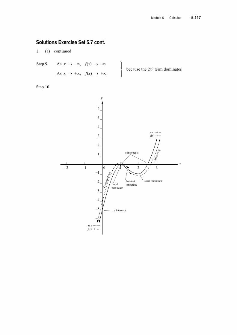
Module 5 – Calculus 5.117
Solutions Exercise Set 5.7 cont.
1. (a) continued
Step 10.
Step 9. As x 2 –,, f(x) 2 –,
As x 2 +,, f(x) 2 +, because the 2x3 term dominates
| | | | |
–2 –1 0 1 2 3
6 _
5 _
4 _
3 _
2 _
1 _
–1 _
–2 _
–3 _
–4 _
–5 _
–6 _
Conca
ve
up
Conca
ve
dow
n
Local minimumPoint of
inflectionLocal
maximum
x intercepts
y intercept
as x→ ∞
f(x) → ∞
as x→ –∞
f(x) → –∞
y
x
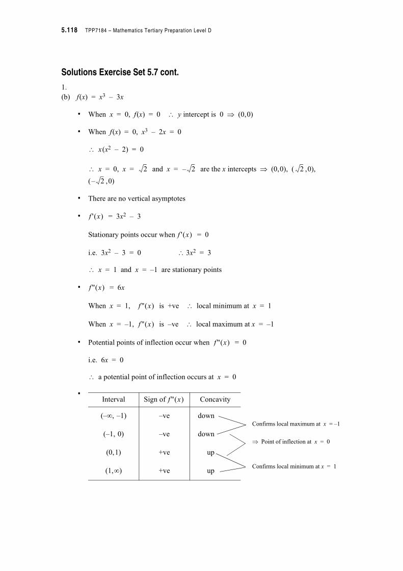
5.118 TPP7184 – Mathematics Tertiary Preparation Level D
Solutions Exercise Set 5.7 cont.
1.
(b) f(x) = x3 – 3x
• When x = 0, f(x) = 0 y intercept is 0 ! (0,0)
• When f(x) = 0, x3 – 2x = 0
x(x2 – 2) = 0
x = 0, x = and x = are the x intercepts ! (0,0), ( ,0),
( ,0)
• There are no vertical asymptotes
• = 3x2 – 3
Stationary points occur when = 0
i.e. 3x2 – 3 = 0 3x2 = 3
x = 1 and x = –1 are stationary points
• = 6x
When x = 1, is +ve local minimum at x = 1
When x = –1, is –ve local maximum at x = –1
• Potential points of inflection occur when = 0
i.e. 6x = 0
a potential point of inflection occurs at x = 0
•
2 2– 2
2–
f ' x" #
f ' x" #
f '' x" #
f '' x" #
f '' x" #
f '' x" #
Interval Sign of Concavity
(–$, –1) –ve down
(–1, 0) –ve down
(0,1) +ve up
(1,$) +ve up
f '' x" #
Confirms local maximum at x = –1
Confirms local minimum at x = 1
! Point of inflection at x = 0
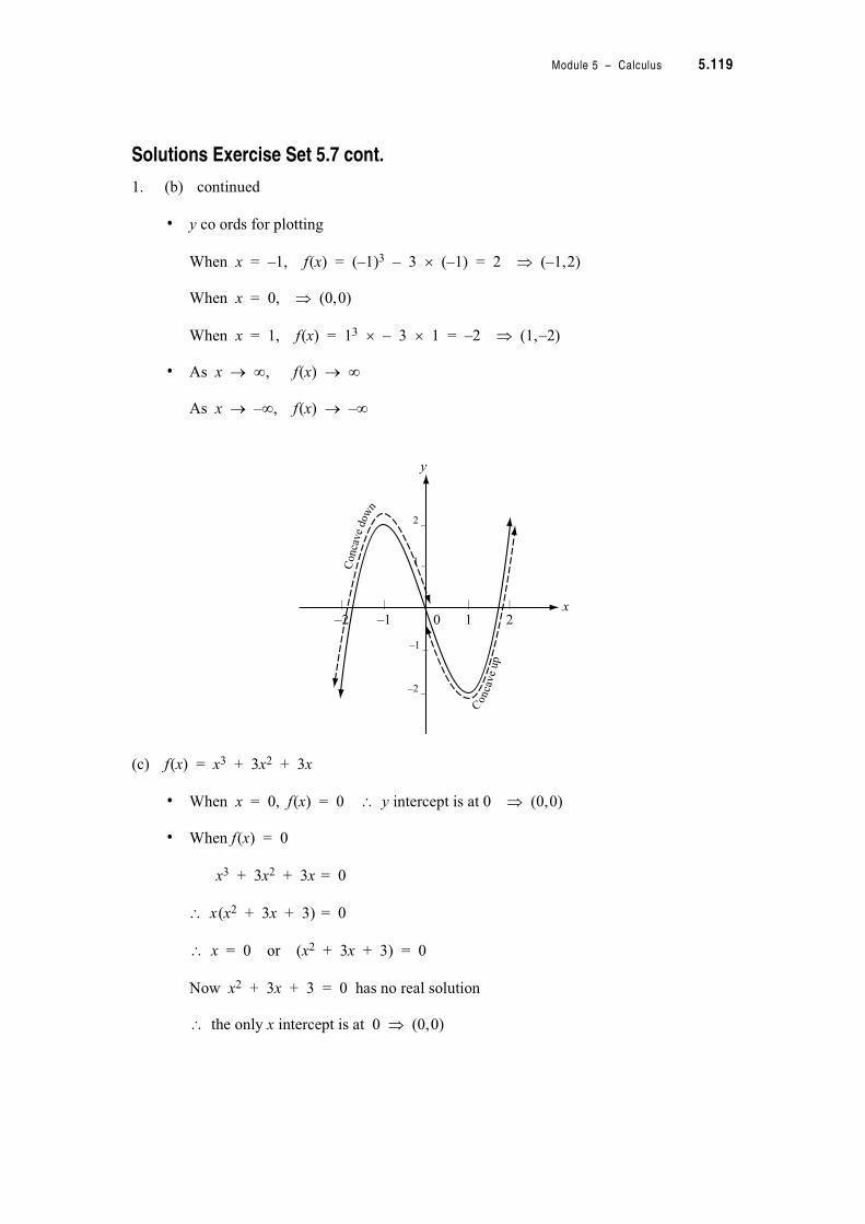
Module 5 – Calculus 5.119
Solutions Exercise Set 5.7 cont.
1. (b) continued
• y co ords for plotting
When x = –1, f(x) = (–1)3 – 3 % (–1) = 2 ! (–1,2)
When x = 0, ! (0,0)
When x = 1, f(x) = 13 % – 3 % 1 = –2 ! (1,–2)
• As x & $, f(x) & $
As x & –$, f(x) & –$
(c) f(x) = x3 + 3x2 + 3x
• When x = 0, f(x) = 0 y intercept is at 0 ! (0,0)
• When f(x) = 0
x3 + 3x2 + 3x = 0
x(x2 + 3x + 3) = 0
x = 0 or (x2 + 3x + 3) = 0
Now x2 + 3x + 3 = 0 has no real solution
the only x intercept is at 0 ! (0,0)
| | | |
–2 –1 0 1 2
2 _
1 _
–1 _
–2 _
C
onca
ve
up
nwod
evac
no
C
x
y

5.120 TPP7184 – Mathematics Tertiary Preparation Level D
Solutions Exercise Set 5.7 cont.
1. (c) continued
• There are no vertical asymptotes
• = 3x2 + 6x + 3
Stationary points occur where = 0
i.e. 3x2 + 6x + 3 = 0
x2 + 2x + 1 = 0
(x + 1)2 = 0
x = –1 is a stationary point
• = 6x + 6
When x = –1, = 0 the second derivative test fails
Try the first derivative test
An x value to the near left of x = –1 is x = –2
= 3 % (–2)2 + 6 % (–2) + 3 which is +ve
An x value to the near right of x = –1 is x = –0.5
= 3 % (–0.5)2 + 6 % (–0.5) + 3 which is +ve
As there has not been a change in the sign of the slope across x = –1, there is no maximum or minimum at x = –1 but there may be a point of inflection.
• Potential points of inflection occur when f''(x) = 0
i.e. 6x + 6 = 0
i.e. at x = –1 {as was expected from above}
f ' x" #
f ' x" #
f '' x" #
f '' x" #
f ' 2–" #
f ' 0.5–" #
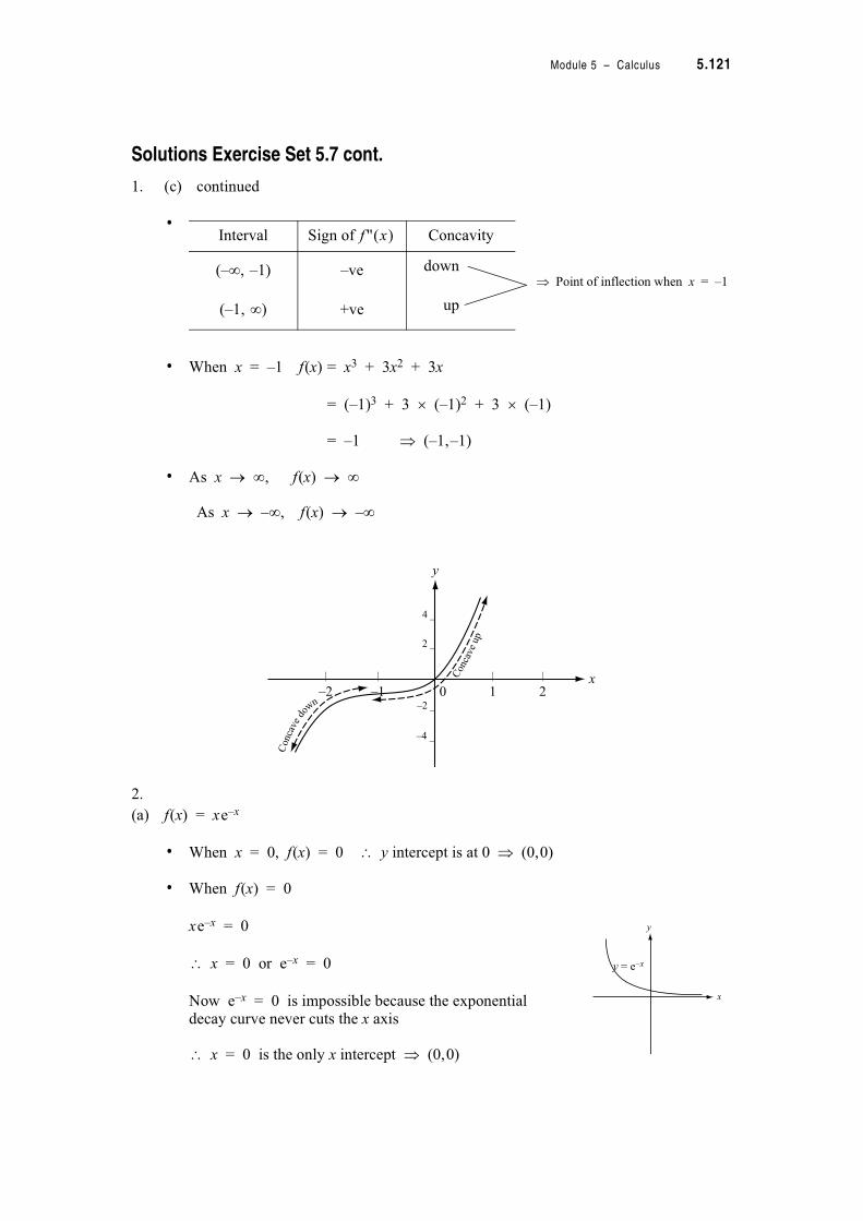
Module 5 – Calculus 5.121
Solutions Exercise Set 5.7 cont.
1. (c) continued
•
• When x = –1 f(x) = x3 + 3x2 + 3x
= (–1)3 + 3 % (–1)2 + 3 % (–1)
= –1 ! (–1,–1)
• As x & $, f(x) & $
As x & –$, f(x) & –$
2.
(a) f(x) = xe–x
• When x = 0, f(x) = 0 y intercept is at 0 ! (0,0)
• When f(x) = 0
xe–x = 0
x = 0 or e–x = 0
Now e–x = 0 is impossible because the exponentialdecay curve never cuts the x axis
x = 0 is the only x intercept ! (0,0)
Interval Sign of Concavity
(–$, –1) –ve down
(–1, $) +ve up
f '' x" #
! Point of inflection when x = –1
| | | |
–2 –1 0 1 2
4 _
2 _
–2 _
–4 _
Conc
ave
do
wn
Con
cave
up
y
x
x
y
y = e–x
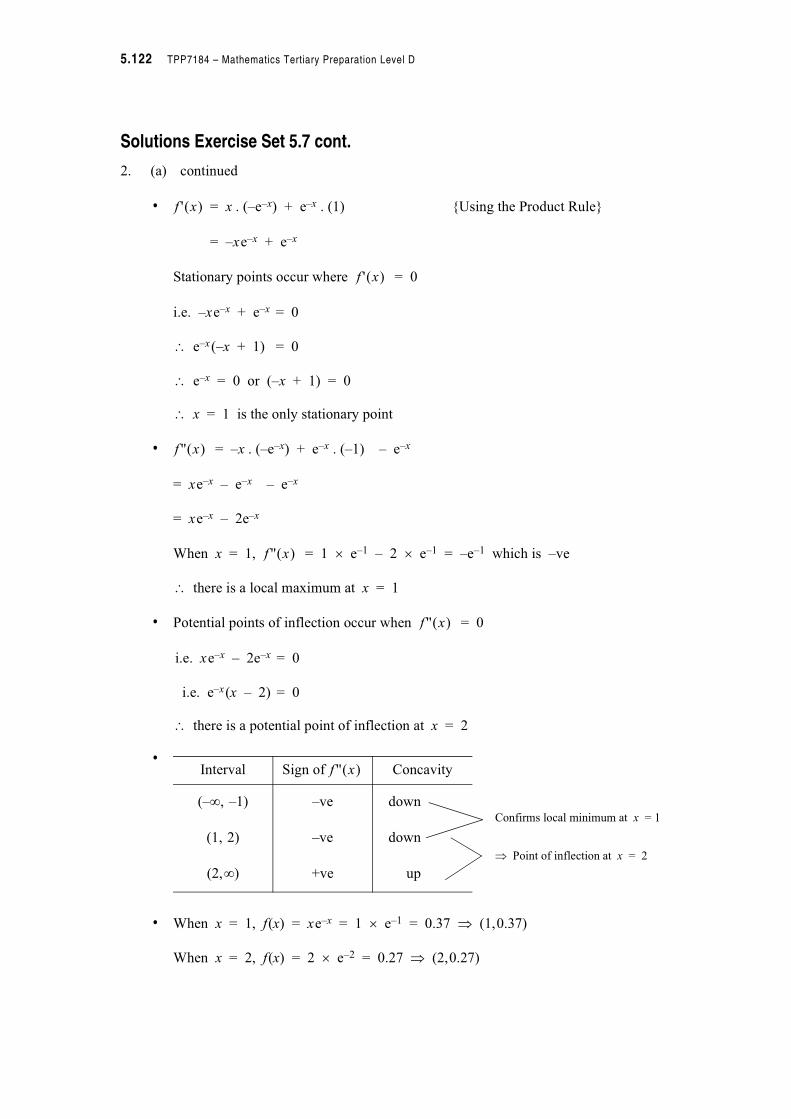
5.122 TPP7184 – Mathematics Tertiary Preparation Level D
Solutions Exercise Set 5.7 cont.
2. (a) continued
• = x . (–e–x) + e–x . (1) {Using the Product Rule}
= –xe–x + e–x
Stationary points occur where = 0
i.e. –xe–x + e–x = 0
e–x(–x + 1) = 0
e–x = 0 or (–x + 1) = 0
x = 1 is the only stationary point
• = –x . (–e–x) + e–x . (–1) – e–x
= xe–x – e–x – e–x
= xe–x – 2e–x
When x = 1, = 1 % e–1 – 2 % e–1 = –e–1 which is –ve
there is a local maximum at x = 1
• Potential points of inflection occur when = 0
i.e. xe–x – 2e–x = 0
i.e. e–x(x – 2) = 0
there is a potential point of inflection at x = 2
•
• When x = 1, f(x) = xe–x = 1 % e–1 = 0.37 ! (1,0.37)
When x = 2, f(x) = 2 % e–2 = 0.27 ! (2,0.27)
f ' x" #
f ' x" #
f '' x" #
f '' x" #
f '' x" #
Interval Sign of Concavity
(–$, –1) –ve down
(1, 2) –ve down
(2,$) +ve up
f '' x" #
Confirms local minimum at x = 1
! Point of inflection at x = 2
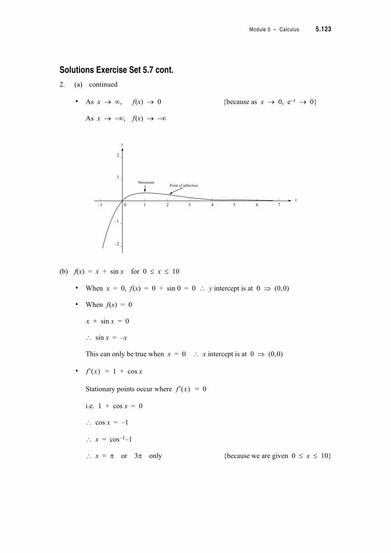
Module 5 – Calculus 5.123
Solutions Exercise Set 5.7 cont.
2. (a) continued
• As x & $, f(x) & 0 {because as x & 0, e–x & 0}
As x & –$, f(x) & –$
(b) f(x) = x + sin x for 0 ' x ' 10
• When x = 0, f(x) = 0 + sin 0 = 0 y intercept is at 0 ! (0,0)
• When f(x) = 0
x + sin x = 0
sin x = –x
This can only be true when x = 0 x intercept is at 0 ! (0,0)
• = 1 + cos x
Stationary points occur where = 0
i.e. 1 + cos x = 0
cos x = –1
x = cos–1–1
x = ( or 3( only {because we are given 0 ' x ' 10}
| | | | | | | |
–1 0 1 2 3 4 5 6 7
2 _
1 _
–1 _
–2 _
MaximumPoint of inflection
y
x
f ' x" #
f ' x" #
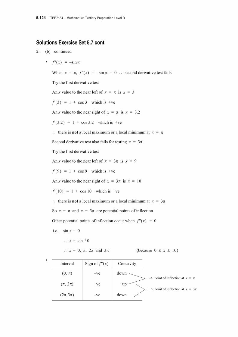
5.124 TPP7184 – Mathematics Tertiary Preparation Level D
Solutions Exercise Set 5.7 cont.
2. (b) continued
• = –sin x
When x = (, = –sin ( = 0 second derivative test fails
Try the first derivative test
An x value to the near left of x = ( is x = 3
= 1 + cos 3 which is +ve
An x value to the near right of x = ( is x = 3.2
= 1 + cos 3.2 which is +ve
there is not a local maximum or a local minimum at x = (
Second derivative test also fails for testing x = 3(
Try the first derivative test
An x value to the near left of x = 3( is x = 9
= 1 + cos 9 which is +ve
An x value to the near right of x = 3( is x = 10
= 1 + cos 10 which is +ve
there is not a local maximum or a local minimum at x = 3(
So x = ( and x = 3( are potential points of inflection
Other potential points of inflection occur when = 0
i.e. –sin x = 0
x = sin–1 0
x = 0, (, 2( and 3( {because 0 ' x ' 10}
•
f '' x" #
f '' x" #
f ' 3" #
f ' 3.2" #
f ' 9" #
f ' 10" #
f '' x" #
Interval Sign of Concavity
(0, () –ve down
((, 2() +ve up
(2(,3() –ve down
f '' x" #
! Point of inflection at x = (
! Point of inflection at x = 3(

Module 5 – Calculus 5.125
Solutions Exercise Set 5.7 cont.
2. (b) continued
Note that this exercise shows that x is always greater than (or equal to) sin x3.
(a) f(x) = x3 – 9x2 – 48x for –5 ' x ' 12
The global maximum and global minimum will occur at either one of end points of the given domain of x or at one of the stationary points in the domain.
= 3x2 – 18x – 48
Stationary points occur when = 0
i.e. 3x2 – 18x – 48 = 0
x2 – 6x – 16 = 0
(x – 8) (x + 2) = 0
x = 8 and x = –2 are stationary points {Check that each of these is in the
given domain before proceeding}
= 6x – 18
When x = 8, = 6 % 8 – 18 which is +ve
there is a local minimum at x = 8
f ' x" #
f ' x" #
f '' x" #
f '' 8" #
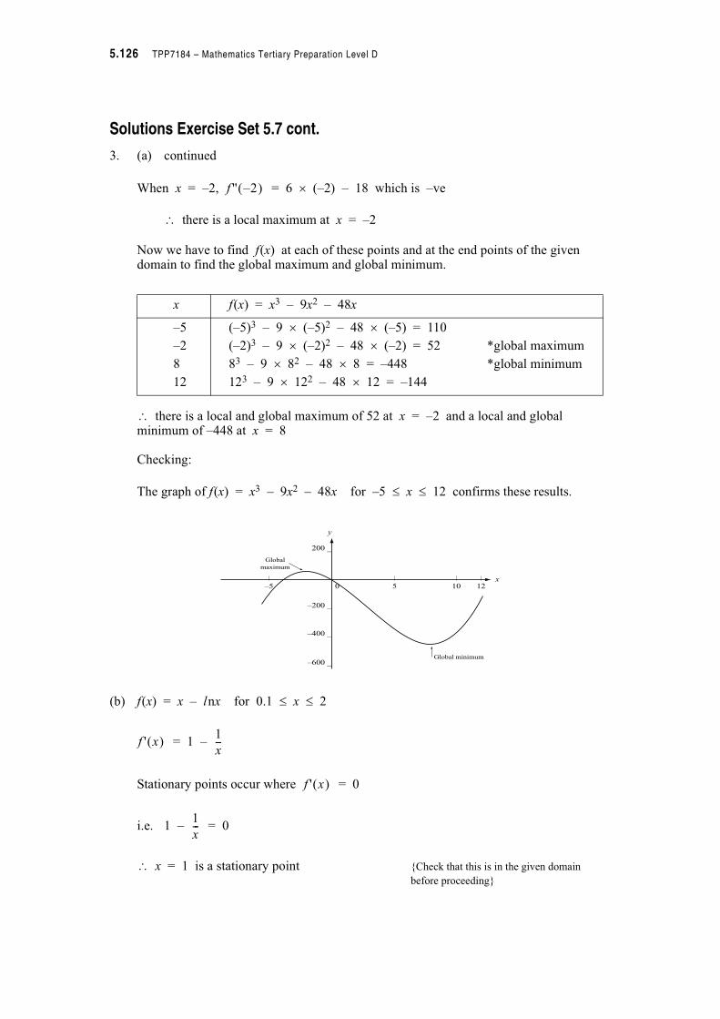
5.126 TPP7184 – Mathematics Tertiary Preparation Level D
Solutions Exercise Set 5.7 cont.
3. (a) continued
When x = –2, = 6 % (–2) – 18 which is –ve
there is a local maximum at x = –2
Now we have to find f(x) at each of these points and at the end points of the given domain to find the global maximum and global minimum.
there is a local and global maximum of 52 at x = –2 and a local and global minimum of –448 at x = 8
Checking:
The graph of f(x) = x3 – 9x2 – 48x for –5 ' x ' 12 confirms these results.
(b) f(x) = x – lnx for 0.1 ' x ' 2
= 1 –
Stationary points occur where = 0
i.e. 1 – = 0
x = 1 is a stationary point {Check that this is in the given domain
before proceeding}
x f(x) = x3 – 9x2 – 48x
–5
–2
8
12
(–5)3 – 9 % (–5)2 – 48 % (–5) = 110
(–2)3 – 9 % (–2)2 – 48 % (–2) = 52 *global maximum
83 – 9 % 82 – 48 % 8 = –448 *global minimum
123 – 9 % 122 – 48 % 12 = –144
f '' 2–" #
| | | |
–5 0 5 10 12
–200 _
200 _
–400 _
–600 _
x
y
Global
maximum
Global minimum
f ' x" #1
x---
f ' x" #
1
x---
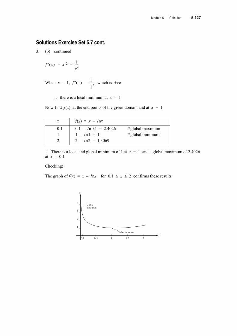
Module 5 – Calculus 5.127
Solutions Exercise Set 5.7 cont.
3. (b) continued
= x–2 =
When x = 1, = which is +ve
there is a local minimum at x = 1
Now find f(x) at the end points of the given domain and at x = 1
There is a local and global minimum of 1 at x = 1 and a global maximum of 2.4026 at x = 0.1
Checking:
The graph of f(x) = x – lnx for 0.1 ' x ' 2 confirms these results.
x f(x) = x – lnx
0.1
1
2
0.1 – ln0.1 = 2.4026 *global maximum
1 – ln1 = 1 *global minimum
2 – ln2 = 1.3069
f '' x" #1
x2-----
f '' 1" #1
12
-----
| | | | |
0.1 0.5 1 1.5 2
4 _
3 _
2 _
1 _
y
x
Global
maximum
Global minimum
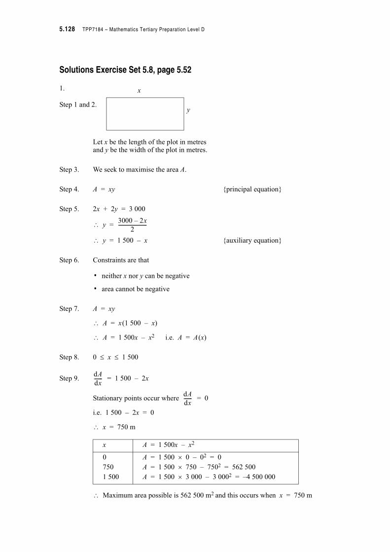
5.128 TPP7184 – Mathematics Tertiary Preparation Level D
Solutions Exercise Set 5.8, page 5.52
1.
Step 1 and 2.
Let x be the length of the plot in metresand y be the width of the plot in metres.
Step 3. We seek to maximise the area A.
Step 4. A = xy {principal equation}
Step 5. 2x + 2y = 3 000
y =
y = 1 500 – x {auxiliary equation}
Step 6. Constraints are that
• neither x nor y can be negative
• area cannot be negative
Step 7. A = xy
A = x(1 500 – x)
A = 1 500x – x2 i.e. A = A(x)
Step 8. 0 ' x ' 1 500
Step 9. = 1 500 – 2x
Stationary points occur where = 0
i.e. 1 500 – 2x = 0
x = 750 m
Maximum area possible is 562 500 m2 and this occurs when x = 750 m
x A = 1 500x – x2
0
750
1 500
A = 1 500 % 0 – 02 = 0
A = 1 500 % 750 – 7502 = 562 500
A = 1 500 % 3 000 – 3 0002 = –4 500 000
x
y
3000 2x–
2------------------------
dA
dx-------
dA
dx-------

Module 5 – Calculus 5.129
Solutions Exercise Set 5.8 cont.
1. continued
Step 10. y = 1500 – x
When x = 750 m
y = 1 500 – 750 = 750 m
Step 11. The farmer should fence a square plot of side length 750 m to enclose the largest possible area of 562 500 m2 with the 3 000 m of fencing available.
2.
Let the perpendicular height of the can be h cm and the radius of the can be r cm.
We are given the volume of the can = 4 000 cm3
We seek to minimise the surface area of the can, A because this will minimise the amount of material used to make the can.
A = 2(rh + 2(r2 {principal equation}
4 000 = (r2h {volume of can is given as 4 000 cm3}
h = {auxiliary equation}
A = 2(rh + 2(r2
= 2(r + 2(r2
A = + 2(r2 i.e. A = A(r)
The absolutely smallest value r can take is zero and the absolutely largest value it can take is achieved when h = 0 but these are not of interest as then the can does not exist. We need to find a local minimum for A.
hh cm
r cm
Note: can is sealed at each end
4000
(r2
------------
4000
(r2
------------) *+ ,
8000
r------------
5.130 TPP7184 – Mathematics Tertiary Preparation Level D
Solutions Exercise Set 5.8 cont.
2. continued
= + 4(r
Stationary points occur when = 0
i.e. + 4(r3 = 0
–8 000 + 4(r3 = 0 {multiplying through by r2, assuming r2 - 0}
r3 =
r = 8.603 cm
Use the second derivative test to show that r = 8.603 cm yields the minimumvalue for A.
= + 4(
When r = 8.603
is +ve minimum at r = 8.603 cm
If r = 8.603 then h = = = 17.203 cm
Now checking that a can with these dimension has a volume of 4 000 cm3
V = (r2h
= ( % 8.6032 % 17.203
. 4 000 cm3 ✓
To minimise the amount of materials needed to make a 4 000 cm3 closed cylindrical can, the height of the can should be 17.203 cm and the radius of the base of the can should be 8.603 cm.
dA
dr-------
8000–
r2
---------------
dA
dr-------
8000–
r2
---------------
8000
4(------------
d2A
dr2
---------16000
r3
---------------
d2A
dr2
---------
4000
(r2
------------4000
( 8.6032%
-------------------------

Module 5 – Calculus 5.131
Solutions Exercise Set 5.8 cont.
3. F =
F = 50c(csin / + cos /)–1
i.e. F is function of a function
Let z = csin / + cos / F = 50cz–1
= ccos / – sin / = –50cz–2
= –50c(csin / + cos /)–2
Now =
= –50c(csin / + cos /)–2 % (ccos / – sin /)
= (1)
For F to be either maximised or minimised when c = tan /, we need to show
that = 0 when c = tan / (i.e. c = )
To force to be zero, the numerator of equation (1) must go to zero.
Numerator of equation (1) is –50c(ccos / – sin /) = –50c2cos / + 50csin /
Substituting c = gives
–50c2cos / + 50csin / = –50 % cos / + 50 % sin /
= –50 + 50
= 0
= 0 when c = tan /
So F is either maximised or minimised when c = tan /.
Note: The force is actually minimised when c = tan /, i.e. the force required to move the object is least when the coefficient of friction equals the tangent of the angle the rope makes with the surface.
θ
50 kg
50c
c /sin /cos+--------------------------------
dz
d/------
dF
dz-------
dF
d/-------
dF
dz-------
dz
d/------0
50c– c /cos /sin–" #
c /sin /cos+" #2-------------------------------------------------
dF
d/-------
/sin
/cos------------
dF
d/-------
/sin
/cos------------
/2
sin
/2
cos--------------
/sin
/cos------------
/2
sin
/cos-------------
/2
sin
/cos-------------
dF
d/-------
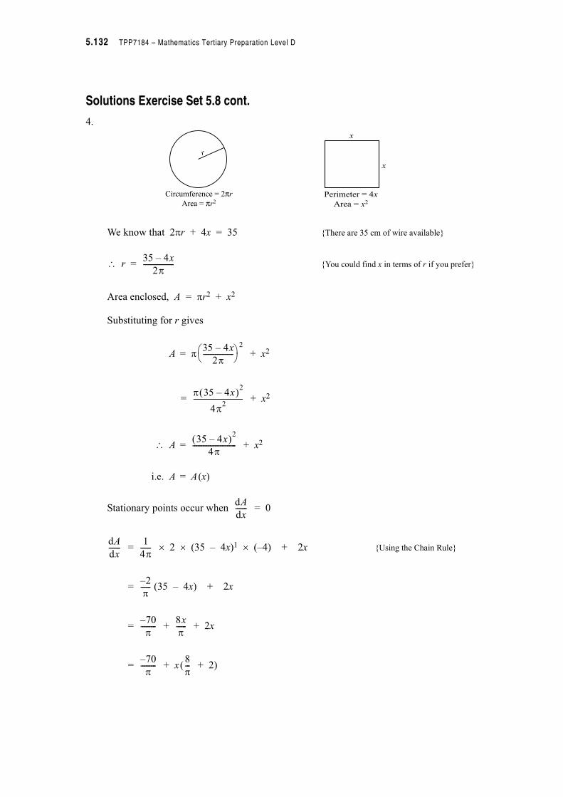
5.132 TPP7184 – Mathematics Tertiary Preparation Level D
Solutions Exercise Set 5.8 cont.
4.
We know that 2(r + 4x = 35 {There are 35 cm of wire available}
r = {You could find x in terms of r if you prefer}
Area enclosed, A = (r2 + x2
Substituting for r gives
A = ( + x2
= + x2
A = + x2
i.e. A = A(x)
Stationary points occur when = 0
= % 2 % (35 – 4x)1 % (–4) + 2x {Using the Chain Rule}
= (35 – 4x) + 2x
= + + 2x
= + x( + 2)
r
Circumference = 2πr
Area = πr2
x
x
Perimeter = 4x
Area = x2
35 4x–
2(------------------
35 4x–
2(------------------) *+ ,
2
( 35 4x–" #2
4(2----------------------------
35 4x–" #2
4(-------------------------
dA
dx-------
dA
dx-------
1
4(------
2–
(------
70–
(---------
8x
(------
70–
(---------
8
(---
Module 5 – Calculus 5.133
Solutions Exercise Set 5.8 cont.
4. continued
When = 0
+ x( + 2) = 0
i.e. x =
= 4.9 cm
Check that when x = 4.9, the area is minimised.
= + 2 which is always +ve minimum area occurs when x = 4.9cm
Now perimeter of square = 4x = 4 % 4.9 = 19.6 cm
Thus the wire should be cut into two pieces with the longer piece of 19.6 cm formed into the square and the shorter piece of 15.4 cm formed into the circle.
dA
dx-------
70–
(---------
8
(---
70
(------
8
(--- 2+) *+ ,
-------------------------------
d2A
dx2
---------8
(---

5.134 TPP7184 – Mathematics Tertiary Preparation Level D
Solutions Exercise Set 5.9 page 5.59
1. f(x) = ex + x – 3
The roots will occur where f(x) = 0
i.e. ex + x – 3 = 0 i.e. ex = –x + 3
If we rewrite this equation as
y1 = ex
and y2 = –x + 3
and then find an approximation of the x co ord of the point of intersection of the graphs of y1 and y2, this will give a good starting point for Newton’s method, i.e. it provides x0
y1 and y2 intersect only once, at about x = 0.8
1f(x) has only one root. Choose x0 = 0.8
| | | | |
–2 –1 0 1 2 3
4 _
3 _
2 _
1 _
–1 _
–2 _
y1 = ex
y2 = –x + 3
x
y
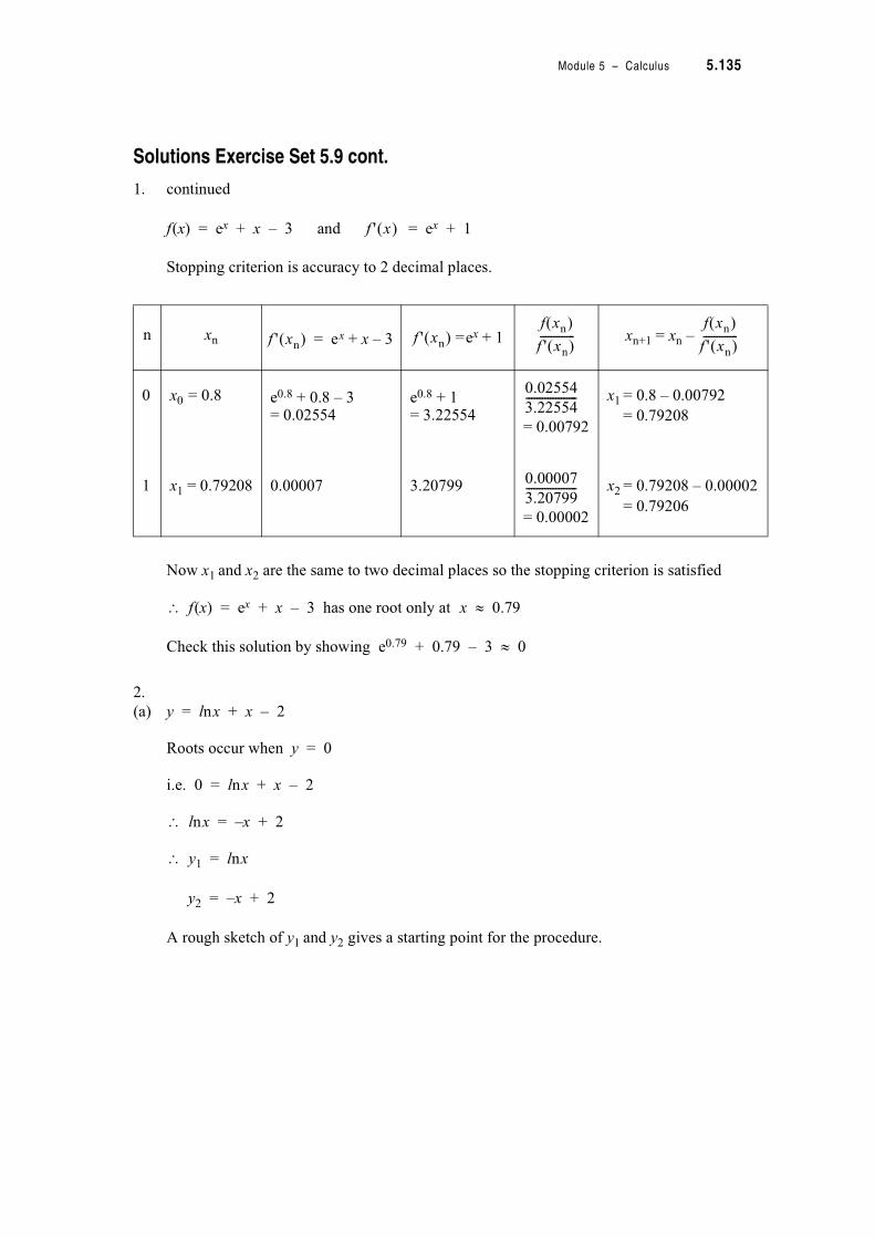
Module 5 – Calculus 5.135
Solutions Exercise Set 5.9 cont.
1. continued
f(x) = ex + x – 3 and = ex + 1
Stopping criterion is accuracy to 2 decimal places.
Now x1 and x2 are the same to two decimal places so the stopping criterion is satisfied
f(x) = ex + x – 3 has one root only at x . 0.79
Check this solution by showing e0.79 + 0.79 – 3 . 0
2.
(a) y = lnx + x – 2
Roots occur when y = 0
i.e. 0 = lnx + x – 2
lnx = –x + 2
y1 = lnx
y2 = –x + 2
A rough sketch of y1 and y2 gives a starting point for the procedure.
n xn =ex + 1 xn+1 = xn –
0 x0 = 0.8 e0.8 + 0.8 – 3= 0.02554
e0.8 + 1= 3.22554
= 0.00792
x1 = 0.8 – 0.00792
= 0.79208
1 x1 = 0.79208 0.00007 3.20799
= 0.00002
x2 = 0.79208 – 0.00002
= 0.79206
f ' x" #
f ' xn" # ex x 3–+= f ' xn" #f xn" #
f ' xn" #-------------
f xn" #
f ' xn" #-------------
0.02554
3.22554-------------------
0.00007
3.20799-------------------

5.136 TPP7184 – Mathematics Tertiary Preparation Level D
Solutions Exercise Set 5.9 cont.
2. continued
There is only one point of intersection of y1 = lnx and y2 = –x + 2 so f(x) has only one root. Choose x0 = 1.5
f(x) = lnx + x – 2 and = + 1
Stopping criterion is accuracy to 2 decimal places.
Now x2 and x1 are the same to two decimal places so the stopping criterion is satisfied
y = lnx + x – 2 has one root only at x . 1.56
Check this solution by showing ln1.56 + 1.56 – 2 . 0
n xn f(xn) = lnx +x–2 = +1 xn+1 = xn –
0 x0 = 1.5 ln1.5 + 1.5 – 2= –0.09453
+ 1
= 1.66667 = –0.05672
x1 = 1.5 – (–0.05672)
= 1.55672
1 x1 = 1.55672 –0.00070 1.64238 = –0.00043 x2 = 1.55672 – (–0.00043)
=1.55715
| | | | |
–1 0 1 2 3 4
2 _
1 _
–1 _
–2 _
y1 = lnx
y2 = –x + 2
x
y
f ' x" #1
x---
f ' xn" #1
x---
f xn" #
f ' xn" #-------------
f xn" #
f ' xn" #-------------
1
1.5-------
0.0945321.66667-----------------------
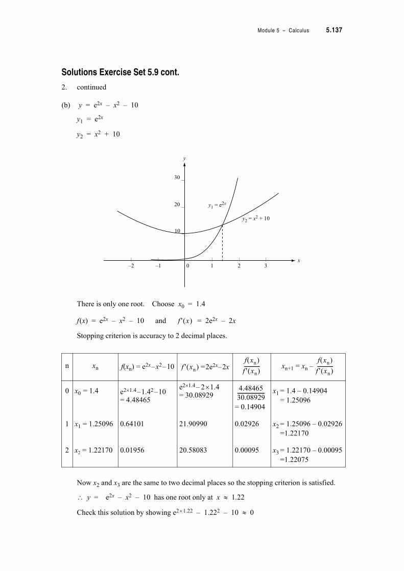
Module 5 – Calculus 5.137
Solutions Exercise Set 5.9 cont.
2. continued
(b) y = e2x – x2 – 10
y1 = e2x
y2 = x2 + 10
There is only one root. Choose x0 = 1.4
f(x) = e2x – x2 – 10 and = 2e2x – 2x
Stopping criterion is accuracy to 2 decimal places.
Now x2 and x3 are the same to two decimal places so the stopping criterion is satisfied.
y = e2x – x2 – 10 has one root only at x . 1.22
Check this solution by showing e2%1.22 – 1.222 – 10 . 0
n xn f(xn) = e2x–x2–10 =2e2x–2x xn+1 = xn –
0 x0 = 1.4 e2%1.4–1.42–10= 4.48465
e2%1.4– 2%1.4= 30.08929
= 0.14904
x1= 1.4 – 0.14904
= 1.25096
1 x1 = 1.25096 0.64101 21.90990 0.02926 x2= 1.25096 – 0.02926
=1.22170
2 x2 = 1.22170 0.01956 20.58083 0.00095 x3= 1.22170 – 0.00095
=1.22075
| | | | |
–2 –1 0 1 2 3
30 _
20 _
10 _
y1 = e2x
y2 = x2 + 10
y
x
f ' x" #
f ' xn" #f xn" #
f ' xn" #-------------
f xn" #
f ' xn" #-------------
4.48465
30.08929----------------------
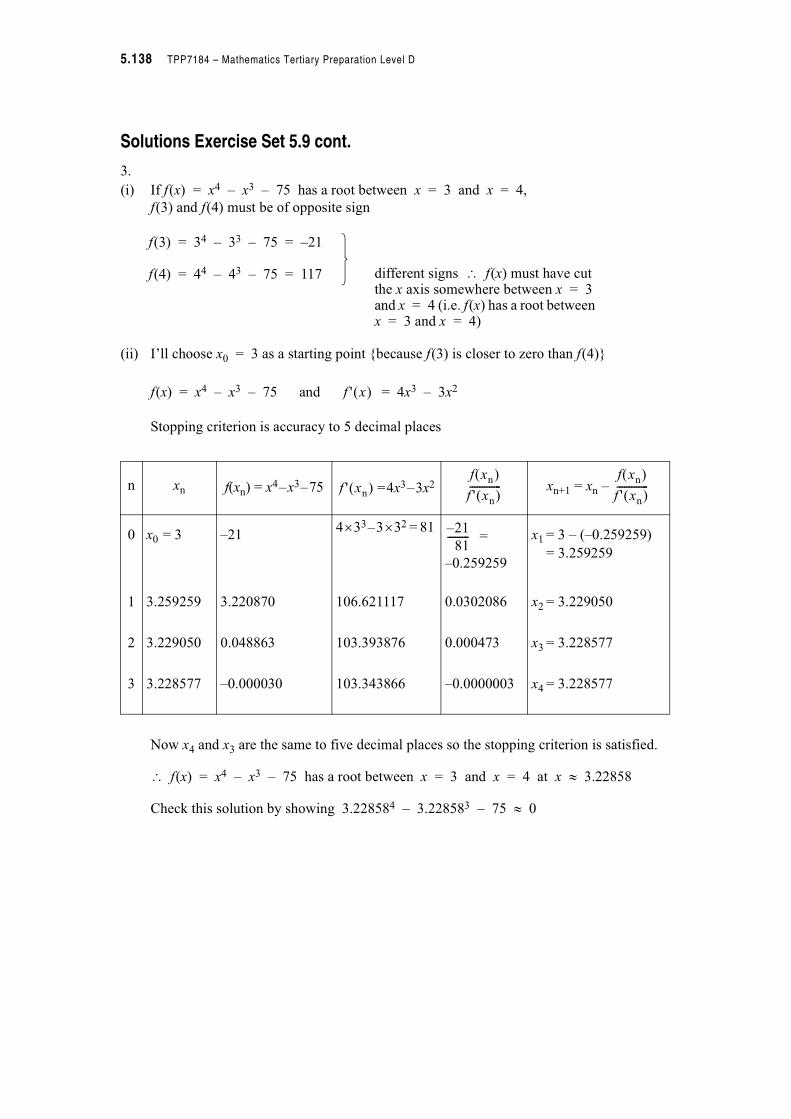
5.138 TPP7184 – Mathematics Tertiary Preparation Level D
Solutions Exercise Set 5.9 cont.
3.
(i) If f(x) = x4 – x3 – 75 has a root between x = 3 and x = 4,
f(3) and f(4) must be of opposite sign
(ii) I’ll choose x0 = 3 as a starting point {because f(3) is closer to zero than f(4)}
f(x) = x4 – x3 – 75 and = 4x3 – 3x2
Stopping criterion is accuracy to 5 decimal places
Now x4 and x3 are the same to five decimal places so the stopping criterion is satisfied.
f(x) = x4 – x3 – 75 has a root between x = 3 and x = 4 at x . 3.22858
Check this solution by showing 3.228584 – 3.228583 – 75 . 0
n xn f(xn) = x4–x3–75 =4x3–3x2 xn+1 = xn –
0 x0 = 3 –214%33–3%32 = 81
=
–0.259259
x1 = 3 – (–0.259259)
= 3.259259
1 3.259259 3.220870 106.621117 0.0302086 x2 = 3.229050
2 3.229050 0.048863 103.393876 0.000473 x3 = 3.228577
3 3.228577 –0.000030 103.343866 –0.0000003 x4 = 3.228577
f(3) = 34 – 33 – 75 = –21
f(4) = 44 – 43 – 75 = 117 different signs f(x) must have cut the x axis somewhere between x = 3 and x = 4 (i.e. f(x) has a root between x = 3 and x = 4)
f ' x" #
f ' xn" #f xn" #
f ' xn" #-------------
f xn" #
f ' xn" #-------------
21–
81---------

Module 5 – Calculus 5.139
Solutions Exercise Set 5.9 cont.
4. Let y1 = cos x
and y2 = x
We can solve these equations using Newton’s method by finding where
cos x = x i.e. by finding where f(x) = cos x – x has a root.
There is only one root. Choose x0 = 0.8
f(x) = cos x – x and = –sin x – 1
Stopping criterion is accuracy to 5 decimal places. Note: Radians must be used.
Now x3 and x2 are the same to five decimal places so the stopping criterion is satisfied.
The x co ord of the point of intersection of y = cos x and y = x isx . 0.73909 and the y co ord at the point of intersection is y . 0.73909
Check this solution by showing cos 0.73909 . 0.73909
n xn f(xn) = cos x – x =–sinx–1 xn+1 = xn –
0 0.8 –0.103293–1.717356 0.060147
x1= 0.739853
1 0.739853 –0.001285 –1.674179 0.000768 x2= 0.739085
2 0.739085 0.0000002 –1.673612 –0.0000001 x3= 0.739085
| | | | | | | | | | | |
–6 –5 –4 –3 –2 –1 0 1 2 3 4 5 6
2 _
1 _
–1 _
y1 = cos x
y2 = x
y
x
f ' x" #
f ' xn" #f xn" #
f ' xn" #-------------
f xn" #
f ' xn" #-------------
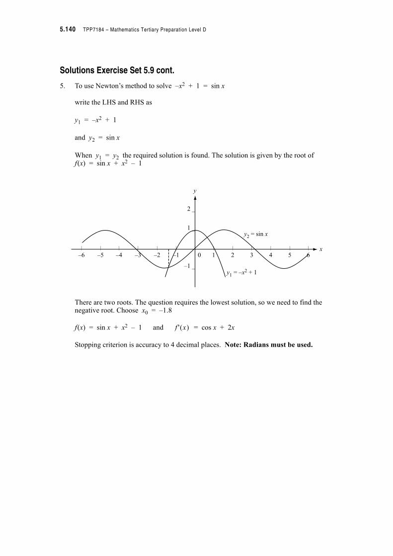
5.140 TPP7184 – Mathematics Tertiary Preparation Level D
Solutions Exercise Set 5.9 cont.
5. To use Newton’s method to solve –x2 + 1 = sin x
write the LHS and RHS as
y1 = –x2 + 1
and y2 = sin x
When y1 = y2 the required solution is found. The solution is given by the root off(x) = sin x + x2 – 1
There are two roots. The question requires the lowest solution, so we need to find the negative root. Choose x0 = –1.8
f(x) = sin x + x2 – 1 and = cos x + 2x
Stopping criterion is accuracy to 4 decimal places. Note: Radians must be used.
| | | | | | | | | | | |
–6 –5 –4 –3 –2 –1 0 1 2 3 4 5 6
2 _
1 _
–1 _
y
x
y1 = –x2 + 1
y2 = sin x
f ' x" #
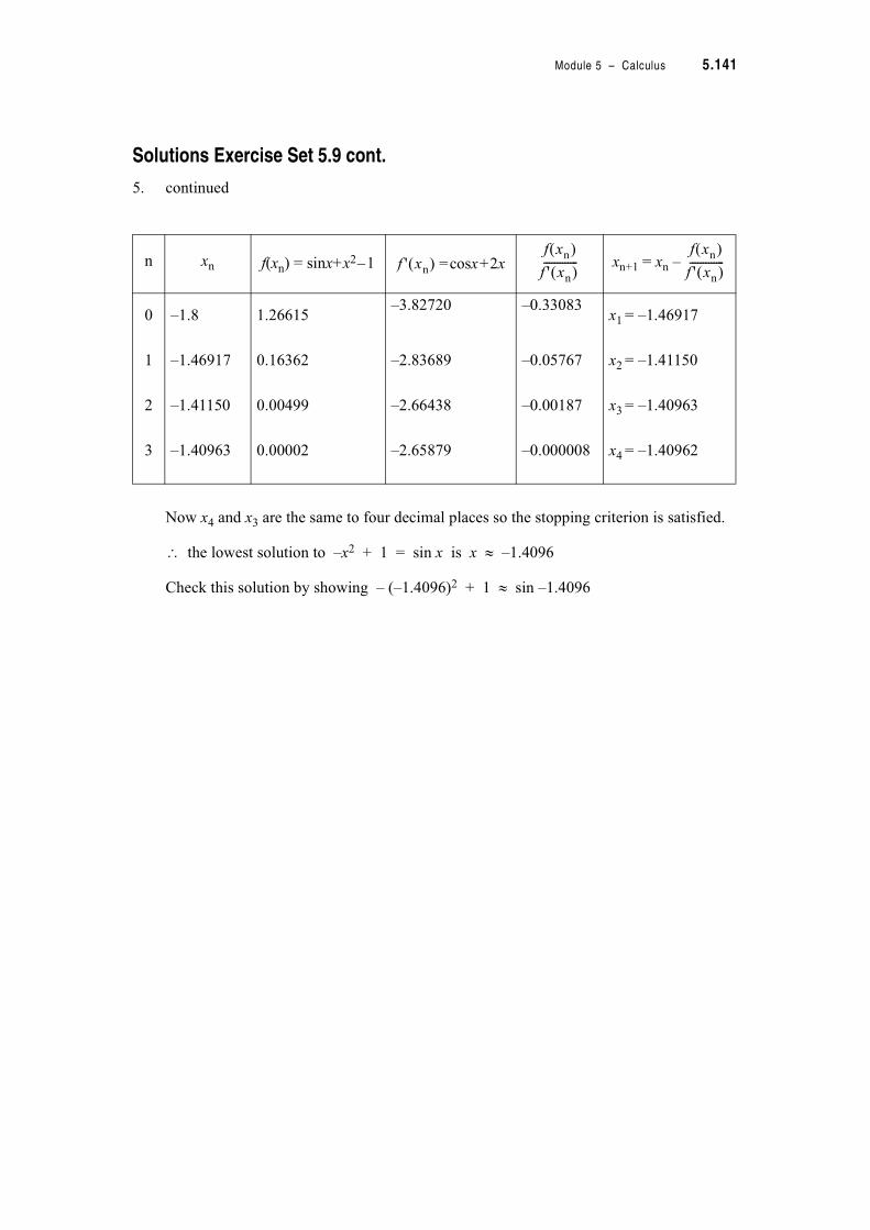
Module 5 – Calculus 5.141
Solutions Exercise Set 5.9 cont.
5. continued
Now x4 and x3 are the same to four decimal places so the stopping criterion is satisfied.
the lowest solution to –x2 + 1 = sin x is x . –1.4096
Check this solution by showing – (–1.4096)2 + 1 . sin –1.4096
n xn f(xn) = sinx+x2–1 =cosx+2x xn+1 = xn –
0 –1.8 1.26615–3.82720 –0.33083
x1= –1.46917
1 –1.46917 0.16362 –2.83689 –0.05767 x2= –1.41150
2 –1.41150 0.00499 –2.66438 –0.00187 x3= –1.40963
3 –1.40963 0.00002 –2.65879 –0.000008 x4= –1.40962
f ' xn" #f xn" #
f ' xn" #-------------
f xn" #
f ' xn" #-------------

5.142 TPP7184 – Mathematics Tertiary Preparation Level D