Module C7

Queuing Models

Basic Concepts

QUEUING MODELS

• Queuing theory is the analysis of waiting lines• It can be used to:

– Determine the # checkout stands to have open at a store– Determine the type of line to have at a bank– Determine the seating procedures at a restaurant– Determine the scheduling of patients at a clinic– Determine landing procedures at an airport– Determine the flow through a production process– Determine the # toll booths to have open on a bridge

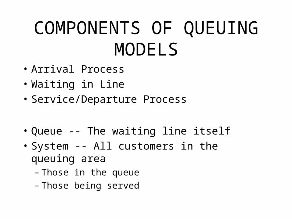
COMPONENTS OF QUEUING MODELS

• Arrival Process

• Waiting in Line

• Service/Departure Process

• Queue -- The waiting line itself

• System -- All customers in the queuing area– Those in the queue– Those being served

The Queue4 customers in the queue

The System7 customers in the system

The Queuing Process1. Customers arrive according to some arrival pattern

2. Customers may have to wait in a queue

3. Customers are served according to some service distribution and depart

ARRIVAL PROCESS

• Deterministic or Probabilistic (how?)

• Determined by # customers in system/balking?

• Single or batch arrivals

• Priority or homogeneous customers

THE WAITING LINE

• One long line or several smaller lines

• Jockeying allowed?

• Finite or infinite line length

• Customers leave line before service?

• Single or tandem queues

THE SERVICE PROCESS

• Single or multiple servers

• Deterministic of probabilistic (how?)

• All servers serve at same rate?

• Speed of service depends on line length?

• FIFO/LIFO or some other service priority

OBJECTIVE

• To design systems that optimize some criteria– Maximizing total profit– Minimizing average wait time for customers– Meeting a desired service level

TYPICAL SERVICE MEASURES

• Average Number of customers in the system -- L

• Average Number of customers in the queue -- Lq

• Average customer time in the system -- W

• Average customer waiting time in the queue -- Wq

• Probability there are n customers in the system -- pn

• Average number of busy servers (utilization rate) --

POISSON ARRIVAL PROCESS

• REQUIRED CONDITIONS– Orderliness

• at most one customer will arrive in any small time interval of t

– Stationarity• for time intervals of equal length, the probability of n

arrivals in the interval is constant

– Independence• the time to the next arrival is independent of when the

last arrival occurred

NUMBER OF ARRIVALS IN TIME t

• Assume = the average number of arrivals per hour (THE ARRIVAL RATE)

• For a Poisson process, the probability of k arrivals in t hours has the following Poisson distribution:

k!

t)( t)in time arrivalsP(k

k te

Time Between Arrivals

• The average time between arrivals is 1/• For a Poisson process, the time between arrivals in

hours has the following exponential distribution:

f(x) = e-t

This means:

P(next arrival occurs > t hours from now) = e-t

P(next arrival occurs within the next t hours) = 1- e-t

POISSON SERVICE PROCESS

• REQUIRED CONDITIONS– Orderliness

• at most one customer will depart in any small time interval of t

– Stationarity• for time intervals of equal length, the probability of completing

n potential services in the interval is constant

– Independence• the time to the completion of a service is independent of when it

started – IS THIS A GOOD ASSUMPTION?

NUMBER OF POTENTIAL SERVICES IN TIME t

• Unlike the arrival process, there must be customers in the system to have services

• Assume = the average number of potential services per hour (SERVICE RATE)

• For a Poisson process, the probability of k potential services in t hours has the following Poisson distribution:

k!

t)( t)in time services potentialP(k

k te

THE SERVICE TIME

• The average service time is 1/• For a Poisson process, the service time has the

following exponential distribution: f(x) = e-t

This means: P(the service will take t additional hours) = e-t

P(the remaining service will take longer than t hours) = 1- e- t

TRANSIENT vs. STEADY STATE

• Steady state is the condition that exists after the system has been operational for a while and wild fluctuations have been “smoothed out”

• Until steady state occurs the system is in a transient state -- transiting to steady state

• It is the long run steady state behavior that we will measure

CONDITIONS FORSTEADY STATE

• For any queuing system to be stable the overall arrival rate must be less than the overall potential service rate, i.e.– For one server: < – For k servers with the same service rate: < k– For k servers with different service rates:

< 1 + 2 + 3 + …+ k

STEADY STATEPERFORMANCE MEASURES

• We’ve mentioned these before:

• Average Number of customers in the system -- L

• Average Number of customers in the queue -- Lq

• Average customer time in the system -- W

• Average customer waiting time in the queue -- Wq

• Probability there are n customers in the system -- pn

• Average number of busy servers (utilization rate) -

Little’s Laws and Other Relationships• Little’s Laws relate L to W and Lq to Wq by:

L = W

Lq = Wq

• Also, (# in Sys) = (# in queue) + (# being served)• Thus• E(# in Sys) = E(# in queue) + E(# being served)

L = Lq +

• Thus knowing one of L, W, Lq and Wq allows us to find the other values.

CLASSIFICATION OF QUEUING SYSTEMS

• Queuing systems are typically classified using a three symbol designation:

(Arrival Dist.)/(Service Dist.)/(# servers)

• Designations for Arrival/Service distributions include:– M = Markovian (Poisson process)– D = Deterministic (Constant)– G = General

Sometimes the designation is extended to 4 or 5 symbols to indicate Max queue length and # in population

M/M/1

• M = Customers arrive according to a Poisson process at an average rate of / hr.

• M = Service times have an exponential distribution with an average service time = 1/ hours

• 1 = one server

• Simplest system -- like EOQ for inventory -- a good starting point

M/M/1PERFORMANCE MEASURES

• Average Number of customers in the system -- L = /(- )

• Average Number of customers in the queue -- Lq = L - /

• Average customer time in the system -- W = L/ • Average customer waiting time in the queue -- Wq = Lq/

• Probability 0 customers in the system -- p0 = 1-/

• Probability n customers in the system -- pn =(/)n p0

• Average number of busy servers (utilization rate) or

Average number customers being served = = /

EXAMPLE -- Mary’s Shoes

• Customers arrive according to a Poisson Process about once every 12 minutes = (60min./hr)/(12 min./customer) = 60/12 = 5/hr.

• Service times are exponential and average 8 min. (service rate) = (60min/hr)/(8min./customer) = 7.5/hr.

• One server• This is an M/M/1 system• Will steady state be reached?

= 5 < = 7.5/hr. YES

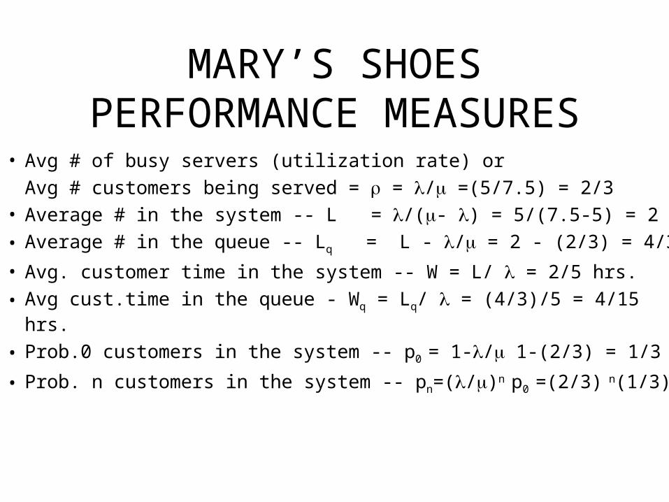
MARY’S SHOESPERFORMANCE MEASURES

• Avg # of busy servers (utilization rate) or

Avg # customers being served = = / =(5/7.5) = 2/3• Average # in the system -- L = /(- ) = 5/(7.5-5) = 2

• Average # in the queue -- Lq = L - / = 2 - (2/3) = 4/3

• Avg. customer time in the system -- W = L/ = 2/5 hrs.

• Avg cust.time in the queue - Wq = Lq/ = (4/3)/5 = 4/15 hrs.

• Prob.0 customers in the system -- p0 = 1-/ 1-(2/3) = 1/3

• Prob. n customers in the system -- pn=(/)n p0 =(2/3) n(1/3)

COMPUTER SOLUTION

• The formulas for an M/M/1 are very simple, but those for other models can be quite complex

• Use M/M/k worksheet in Queue Template– Results are in the row corresponding to 1 server

Steady State ResultsPn’s

Input and

M/M/k SYSTEMS

• M = Customers arrive according to a Poisson process at an average rate of / hr.

• M = Service times have an exponential distribution with an average service time = 1/ hours regardless of the server

• k = k IDENTICAL servers

M/M/k PERFORMANCE MEASURES

02

1

0

0

!1

!1

!1

1

e.g.complex moremuch Formulas•

pkk

L

kk

kn

p

k

k

n

kn

EXAMPLELITTLETOWN POST OFFICE

• Between 9AM and 1PM on Saturdays:– Average of 100 cust. per hour arrive according to a

Poisson process -- = 100/hr.– Service times exponential; average service time =

1.5 min. -- = 60/1.5 = 40/hr.– 3 clerks; k = 3

• This is an M/M/3 system = 100/hr < 3( = 40/hr.) i.e. 100 < 120 – STEADY STATE will be reached

Solution

Using the formulas, with = 100, = 40, k = 3• Prob.0 customers in the system -- p0 = .044944

• Average # in the system -- L = 6.0112

• Average # in the queue -- Lq = 3.5112

• Avg. customer time in the system -- W = .0601 hrs.

• Avg cust.time in the queue - Wq = .0351hrs.

• Avg # of busy servers = = / =(100/40) = 2.5

• Average system utilization rate = /k = 100/120=.83

Input and Performance Measuresfor 3 servers

Pn’s

M/G/1 Systems

• M = Customers arrive according to a Poisson process at an average rate of / hr.

• G = Service times have a general distribution with an average service time = 1/ hours and standard deviation of hours (1/ and in same units)

• 1 = one server

• Cannot get formulas for pn but can get performance measures

Example -- Ted’s TV Repair

• Customers arrive according to a Poisson process once every 2.5 hours --– = 1/2.5 = .4/hr.

• Repair times average 2.25 hours with a standard deviation of 45 minutes = 1/2.25 = .4444/hr. = 45/60 = .75 hrs.

• Ted is the only repairman: k= 1

• THIS IS AN M/G/1 SYSTEM

Performance Measures

• P0 = 1-/ = 1-(.4/.4444) = .0991

• L = (()2 + (/ )2)/(2(1-/ )) + /

= ((.4)(.75)2 + (.4/.4444)2)/(2(.0991)) + (.4/.4444)

= 5.405

• Lq = L - / = 5.405 - .901 = 4.504

• W = L/ = 5.405/.4 = 13.512 hrs.

• Wq = Lq/ = 4.504/.4 = 11.262 hrs.

There are no formulas for the pn’s.

Select MG1 Worksheet

Input (in customers/hr.) (in customers/hr.)

(in hours)

PerformanceMeasures

FINITE QUEUES (M/M/k/F)

• Frequently there are systems that have limits to the maximum number of customers in the system F

• Thus with probability pF the system is FULL and an arriving customer cannot join the queue-- i.e. we lose pF portion of the potential customers

• The effective arrival rate is then e = (1 - pF)

• Use e to calculate L, Lq, W, and Wq

Steady state will always be achieved regardless of and since the queue cannot build up indefinitely!!

Example -- Ryan’s Roofing

• Customer calls average 10/hr.

• 1 server -- average service time -- 3 minutes = 60/3 = 20/hr.

• 3 lines so 2 can be on hold -- they will hold until they are served

• Arriving phone call when all 3 lines busy will not join the system

Select MMkF Worksheet

Input , , k, F

Performance Measurespn’s

e = (1-.06667)(10) = 9.33333 W = L/ e

M/M/1 QUEUES WITH FINITE CALLING POPULATIONS

(M/M/1//m)• Maximum m school buses at repair facility,

or m assigned customers to a salesman, etc.

• 1/ = average time between repeat visits for each of the m customers = average number of arrivals of each

customer per time period (day, week, mo. etc.)

• 1/ = average service time = average service rate in same time units as

Example -- Pacesetter Homes

• 4 projects m = 4

• Average 1 work stoppage every 20 days/project– “arrival” rate of work stoppages, = 1/20 = .05/day

• Average 2 days to resolve work stoppage dispute– “service” rate, = 1/2 = .5/day

Select MM1 m Worksheet

Input , , m

Performance Measurespn’s

Module C7 Review

• Components of a queuing system– Arrivals, Queue, Services

• Assumptions for Poisson (Markovian) distribution

• Requirements for Steady State– Overall service rate > Overall arrival rate

• Steady State Performance Measures– L, Lq, W, Wq, pn’s,

• Queuing Systems– M/M/1, M/M/k, M/G/1, M/M/k/F, M/M/1//m

• Use of the Queue Template