Embed Size (px)
Citation preview
Module 2 – Algebra & Geometry
Module 2
ALGEBRA AND GEOMETRY2

Table of Contents 2.1 Inequalities and the Real Number Line ................................................................. 2.1
Representing Numbers Using the Real Number Line ................................................. 2.1 Operations on Inequalities .......................................................................................... 2.5 Linear Inequalities of Two Variables ......................................................................... 2.7
2.2 Quadratic Equations and Completing the Square .................................................. 2.15 Factorising ................................................................................................................... 2.15 Completing the Square ................................................................................................ 2.20
2.3 Functions ............................................................................................................... 2.28 Polynomials ................................................................................................................. 2.28 Rational Functions ...................................................................................................... 2.33 Decomposition of Proper Rational Functions into Partial Fractions .......................... 2.36 Other Important Non Linear Functions ....................................................................... 2.47 Solving Simultaneous Equations Algebraically and Graphically ............................... 2.56 Inverse Functions ........................................................................................................ 2.61 Continuity ................................................................................................................... 2.69
Solutions to Exercise Sets ............................................................................................... 2.75

Module 2 – Algebra & Geometry 2.1
2.1 Inequalities and the Real Number Line
Representing Numbers Using the Real Number Line
The real number system can be represented by a real number line. i.e. a line which has an infinite (i.e. uncountable) number of numbers ordered so as to show the difference between each number and zero.
Both rational and irrational numbers can be shown on the number line although for the irrational numbers an approximation must be made. This is because we can only define an irrational number in terms of the interval between two rational numbers.
e.g. lies between 1 and 2 or lies between 1.4 and 1.5 or lies between 1.41 and 1.42
or lies between 1.414 and 1.415
Note that the set of rational numbers and the set of irrational numbers together make up the set of real numbers i.e. they make an infinitely ‘dense’ set which can be represented by a continuous line on a page. The real number line is a very useful geometric representation of the real number system as you shall soon see.
An inequality (sometimes called an inequation) is a relationship which holds between two numbers or algebraic expressions which are not equal. There are four symbols which you need to be able to interpret.
Two other symbols you need to know are
which means ‘not equal to’, andwhich means ‘approximately equal to’.
‘less than’
‘less than or equal to’
‘greater than’
‘greater than or equal to’
<
!
>
"
e.g.
e.g.
e.g.
e.g.
x ! 1
1 " x
‘one is less than root two’
‘x is less than one or equal to one’
‘root two is greater than one’
‘one is greater than x or equal to x’
#e32
2
10–1$2
–1–2–3–2.444 ……–% + %
2 2 2
2
1 2&
2 1'
(

2.2 TPP7184 – Mathematics Tertiary Preparation Level D
Exercise Set 2.1
Complete the following by inserting the appropriate symbol between each LHS and RHS.
Consider the inequality x " 1. Why is this statement and the statement 1 ! x equivalent?
.....................................................................................................................................................
.....................................................................................................................................................
Answer:
One way to check this equivalence is to use the real number line. Defining x " 1 on the real number line gives:
LHS RHS
(a)
(b)
(c)
(d)
(e)
–1$ 4
#
0.00012
2.7
0.25
22$ 7
1.2 ) 10–4
e
2– 3–
–% –5 –4 –3 –2 –1 0 1 2 3 4 5 …x " 1
Any real number which lies on this part of the real number line satisfies the inequality
To show that the number 1 satisfies the equality use a square bracket. In some books a filled-in circle, like this, ! , is used. We will use the bracket form.
… + %
[

Module 2 – Algebra & Geometry 2.3
Defining 1 ! x on the real number line gives the same set of numbers because 1 is the lowest possible value that x can be.
So the solution to the inequality x " 1 (or 1 !* x) is any real number greater than or equal to 1.
■
Sometimes inequalities are combined because of certain constraints on the variable of interest.
e.g. –1 < x ! 4 means the solution set for x consists of all the real numbers between –1 and 4 and includes 4.
On the real number line we get
When we are representing the solution sets of variables on the real number line we are actually drawing a one dimensional graph. Later we will show the solution sets of inequalities involving two variables on two dimensional graphs (i.e. the typical XY graph of the Cartesian system).
Check now that you have grasped the idea of inequalities and their solution sets.
–% –5 –4 –3 –2 –1 0 1 2 3 4 5 + %
1 ! x[… …
… –5 –4 –3 –2 –1 0 1 2 3 4 5 + %
–1 < x ! 4 ](–% …
Use a round bracket to show that the number –1 is not included

2.4 TPP7184 – Mathematics Tertiary Preparation Level D
Exercise Set 2.2
Fill in the missing parts of the statements and give a couple of examples of rational and irrational numbers that satisfy each inequality.
1. x ! 4 has the solution set ‘any real number ........................................... 4’ or in intervalnotation, (–%, 4] See Note 1
e.g. –180, , –#, 2, 2.41, #, e, ,
2. –2 < y has the solution set ‘any real number ......................................... 2’ or in intervalnotation, (–2, )
e.g...........................................................................................................................................
3. –½ ! p ! 3 has the solution set ‘ .....................................................................................’or in interval notation [ , ]
e.g...........................................................................................................................................
Why do you think inequalities such as (a) 1 < x > 3 or (b) 1 > x < 4 are nonsense and have no meaning?
.....................................................................................................................................................
.....................................................................................................................................................
Answer:
(a) 1 cannot be greater than 3
(b) x cannot be greater than 4, nor can 4 be less than 1
If in (b) you really wanted x defined so that 1 > x and x < 4 you would need two separate inequalities. 1 > x means x is any number less than 1 or in interval notation (–%, 1)
Notes
1. If a solution set extends to positive or negative infinity, a round bracket is used on the relevant end of the interval.
7–10
3------ 2
–% … … + %
(1 > x
–4 –3 –2 –1 0 1 2 3 4–5 5

Module 2 – Algebra & Geometry 2.5
x < 4 means x is any number less than 4 or in interval notation (–%, 4)
By examining these graphs you should be able to see that if both the inequalities are to be satisfied the solution set is (–%, 1).
Operations on Inequalities
The same rules you use for rearranging or manipulating equations can also be used for inequalities except for the two important cases shown below.
Exception 1: Multiplying or dividing by a negative number.
Consider the equation
–2x = 3
Dividing each side by –2 gives
You can check this is true by selecting a value for x from the solution set (– 3$2, %) and substituting in –2x < 3.
e.g. say x = 4
when x = 4, –2x < 3 gives –2 ) 4 < 3 i.e. –8 < 3 which is valid.
However if we had not changed the sign of the inequality we would get x < – 3$2 as the solution set and choosing a value from this for checking, say x = –6 and substituting in–2x < 3 gives –2 ) –6 < 3 i.e. 12 < 3 which is nonsense.
So the first exception to be remembered when solving inequalities is:
If you divide (or multiply) an inequality by a negative number change the direction of the inequality.
–% … –4 –3 –2 –1 0 1 2 3 4 … %–5
(
5x < 4
x3–
2------=
Note the change in direction of the inequality
x3–
2------'
Consider the inequality
–2x < 3
Dividing each side by –2 gives

2.6 TPP7184 – Mathematics Tertiary Preparation Level D
Exception 2: Inverting two numbers
Consider the inequality
8 > 4
Inverting each side gives
Example 2.1: Find the solution of
2x + 4 ! 3x – 3
Solution:
2x – 3x ! –3 – 4 (Subtract 3x from each side and subtract 4 from each side)
–x ! –7 (Simplify)
x " 7 (Divide by –1 + change of direction inequality)
Check solution by choosing a value for x in the interval [7, +%) and a value not in this interval e.g. Choose say x = 10 and x = 5 See Note 1
When x = 10, 2x + 4 = 2 ) 10 + 4 = 24 and 3x – 3 = 3 ) 10 – 3 = 27 and now
LHS = 24 which is less than RHS = 27 + solution is valid
When x = 5, 2x + 4 = 2 ) 5 + 4 = 14 and 3x – 3 = 3 ) 5 – 3 = 12 and now
LHS = 24 which is not less than RHS = 12 + solution is not valid
If you invert each side of the inequality, change the direction of the inequality.
Notes
1. Choosing any two values like these does not prove the solution is correct but it does provide a checking mechanism.
1
8---
1
4---&
Note the change in direction of the inequality

Module 2 – Algebra & Geometry 2.7
Exercise Set 2.3
Solve the following inequalities.
Express each solution set using the inequality symbols and in interval notation.
1. 2x + 4 ! 8
2. –½ p > 2p + 4
3. 2d + 2 ! 4d – 3
4. 3y – 2 " 4y + 6
5. 2y(3 – y) > (6 – y) (3 + 2y)
6.
Linear Inequalities of Two Variables
These type of inequalities frequently arise in ‘product mix’ type problems where a company wants to maximise profit (or minimise cost) for making certain products to meet the market demand but where there are constraints on the amount of raw materials, production capacity (machinery or labour) etc. Here’s a typical example: See Note 1
Example 2.2:
The Nabnot biscuit Company makes two types of cracker biscuits, ‘Water Biscuits’ and ‘Cheese Dippers’. Biscuit production involves three processes: mixing, cooking and packing. Each batch of ‘Water Biscuits’ requires 3 minutes mixing, 5 minutes cooking and 2 minutes to pack while each batch of ‘Cheese Dippers’ requires 3 minutes mixing, 4 minutes cooking and 3 minutes to pack. The net profit on each batch of ‘Water Biscuits’ is $120 and on each batch of ‘Cheese Dippers’ is $100. If the mixer, oven and packer are only available for 4 hours, 7 hours and 3 hours per day respectively, how much of each type of biscuit should be made daily in order to maximise profit?
Notes
1. Product mix problems are one type of linear programming problems. These problems are an important part of the
branch of mathematics known as Operations Research.
2x 4+ 3&

2.8 TPP7184 – Mathematics Tertiary Preparation Level D
Solution: We want to maximise profit, P subject to certain restrictions in the production plant.
1. Define the profit function:
P = 120x + 100y where x is the number of batches of ‘Water Biscuits’ made daily and y is the number of batches of ‘Cheese Dippers’ made daily.
Note that x and y can never be negative as it doesn’t make sense to produce a negative number of batches. Geometrically these non negativity constraints restrict the solution set to the first quadrant of the Cartesian plane.
2. Establish the constraints:
Mixing:
• one batch of ‘Water Biscuits’ takes 3 minutes mixing, so x batches take 3x minutes
• one batch of ‘Cheese Dippers’ takes 3 minutes mixing, so y batches take 3y minutes
• the mixer is available only for 4 hours (i.e. 240 minutes) per day, so the time taken for mixing the x batches of ‘Water Biscuits’ (i.e. 3x) plus the time taken for mixing the y batches of ‘Cheese Biscuits’ (i.e. 3y) cannot exceed 240 minutes.
i.e. 3x + 3y ! 240 _______________________ "
If all the mixer time was used this inequality would become the equality 3x + 3y = 240.
Use your computer to draw the graph of 3x + 3y = 240. Note: You need to rearrange the formula as y = 80 – 3x. The region defined by the inequality 3x + 3y ! 240 is that to the lower left of the line you have just drawn. (Check this is true by selecting a couple of values for (x, y) that are in this region and algebraically showing that 3x + 3y is indeed less than or equal to 240.)
y110
80
080 90
3x + 3y ! 240
x

Module 2 – Algebra & Geometry 2.9
Cooking:
• one batch of ‘Water Biscuits’ takes 5 minutes cooking, so x batches take 5x minutes
• one batch of ‘Cheese Dippers’ takes 4 minutes cooking, so y batches take 4y minutes
• the oven is available only for 7 hours (i.e. 420 minutes) per day, so the time taken for cooking x batches of ‘Water Biscuits’ (i.e. 5x) plus the time taken for cooking y batches of ‘Cheese Dippers’ (i.e. 4y) cannot exceed 480 minutes.
i.e. 5x + 4y ! 480 _______________________ #
If all the oven time was used this inequality would become the equality 5x + 4y = 420.
Using the same scale and without clearing the screen draw the graph of 5x + 4y = 420 You will now see that the solution set for 5x + 4y ! 420 includes all the points to the lower left of the line 5x + 4y = 420. (For this particular problem it is interesting to note that the first constraint defines a region which is a subset of the region defined by the second constraint.)
Packing:
• one batch of ‘Water Biscuits’ takes 2 minutes to pack, so x batches take 2x minutes
• one batch of ‘Cheese Dippers’ takes 3 minutes to pack, so y batches take 3y minutes
• the packing line is available only for 3 hours (i.e. 180 minutes) per day, so the time taken to pack x batches of ‘Water Biscuits’ and y batches of ‘Cheese Dippers’ cannot exceed 180 minutes
i.e. 2x + 3y ! 180 _______________________ $
Without clearing the current screen on your computer, draw the graph of 2x + 3y = 180
Now you can see how the addition of constraint $ has reduced the possible values of (x, y) that can be in the solution set.
x
110
105
80 840
80
110
y
3x + 3y ! 240
5x + 4y ! 480

2.10 TPP7184 – Mathematics Tertiary Preparation Level D
The solution set of (x, y) which satisfies
3x + 3y ! 240
5x + 4y ! 480
2x + 3y ! 180
and also x ! 0 and y ! 0 (i.e. non negativity constraints) are all the (x, y) points in the region OABC.
3. Find optimal solution:
The final step in this type of optimisation problem to find the maximum value of the profit function in the region defined by the constraints. I will not prove it here, but it turns out that the profit function will be maximised at one of the ‘corner points’ of OABC i.e. at
O (0, 0); A (0, 60); B (60, 20) or C (80, 0) See Note 1
Substituting these values for (x, y) into P = 120x + 100y gives:
At O: when x = 0 and y = 0, P = 120 ) 0 + 100 ) 0 = $0
At A: when x = 0 and y = 60, P = 120 ) 0 + 100 ) 60 = $6 000
At B: when x = 60 and y = 20, P = 120 ) 60 + 100 ) 20 = $9 200
At C: when x = 80 and y = 0, P = 120 ) 80 + 100 ) 0 = $9 600 *optimum
So given the constraints on the system, profit will be maximised at $9 600 per day when 80 batches of ‘Water Biscuits’ and no batches of ‘Cheese Dippers’ are made.
Check your understanding of optimising a function given certain constraints by completing the missing parts of the solution to the following problem.
Notes
1. You can find the coordinates of the corner points by solving the relevant pairs of equations or using the Zoom function on the computer graphing package.
110
70
50
A
90
5x + 4y = 480
3x + 3y = 240
O C70503010
10
30
90
y
B
x2x + 2y = 180

Module 2 – Algebra & Geometry 2.11
Example 2.3:
A dietician is planning the menu for the evening meal at a hospital. Two main items, each having different nutritional content, will be served. Certain minimum daily vitamin requirements are to be met by this meal while the cost of the meal is kept as low as possible. Determine the amount of each food to be included in the meal given the following information.
We want to minimise cost, subject to the daily requirement constraints and the serving size constraint.
1. Definition of Cost Function
C = 3x + 5y where x is the number of 10 gram serves of Food 1
and y is the ...............................................................
2. Establish the non negativity constraints
x " 0y " 0
Establish the vitamin daily requirement constraints
Vitamin 1: x + 30 " 290 (At least 290mg of Vitamin 1must be included)
Vitamin 2: x + " 200 (At least 200mg of Vitamin 2must be included)
Vitamin 3: + " 210 ( ..................................................
...................................................)
So the complete problem is
Minimise C = 3x + 5y
Under the constraints
50x + 30y " 290 __________________ "
20x + 10y " 200 __________________ #
10x + 50y " 210 __________________ $
x " 0 ; y " 0
Vitamin 1 per 10g Vitamin 2 per 10g Vitamins 3 per 10g Cost per 10g
Food 1Food 2
50mg30mg
20mg10mg
10mg50mg
3 cents5 cents
Min. DailyVitaminRequirement
290mg 200mg 210mg
20
y

2.12 TPP7184 – Mathematics Tertiary Preparation Level D
3. Find the set of (x, y) values that satisfies all the constraints. Use your graphing package to draw each constraint as an equality. Use the same screen for all the constraints.
50x + 30y = 290 ______________ " i.e.
Values of (x, y) that satisfy 50x + 30y " 290 will lie to the upper right of the line
x + y = (because of the direction of the inequality).
20x + 10y = 200 ______________ # i.e. y = 20 – 2x
Values of (x, y) that satisfy 20x + 10y " 200 will lie to the ........................... of
the line 20 + y = 200
10x + 50y = 210 ______________ $ i.e. y = – x
Values of ( , ) that satisfy 10x + 50y 210 will lie to the upper right of
the line x + y = 210
The set of (x, y) values that satisfies all the constraints is the region (to the upper right) defined by DEF and the x and y axes
y29
3------
5
3---x–=
EF
y
#
"
$
x

Module 2 – Algebra & Geometry 2.13
4. Find the minimum value of the cost function for this set of (x, y) values. (Recall that theoptimum always occurs at a corner point of the defined region.)
C = 3x + 5y
At D: when x = 0 and y = 20, C = 3x + 5y = 3 ) 0 + 5 ) 20 = 100 cents
At E: when x = 8.78 and = 2.44,C = 3x + 5y = 3 ) + 5 ) = 38.5 cents *optimum
At F: when = and y = 0, C = 3x + 5y = ) 21 + ) 0 = 63 cents
5. Conclusion
So the specifications for the nutritional requirements will be satisfied when 8.8 ‘10 gram serves i.e. 88 grams of Food 1 and 2.4 ‘10 gram serves’ i.e. 24 grams of Food 2 are served. The cost of the diet will then be minimised at 38.5 cents per meal.

2.14 TPP7184 – Mathematics Tertiary Preparation Level D
Exercise Set 2.4
1. Shade the region on the Cartesian Plane in which the solution to these inequalities lies.
(a) 4x + 5y ! 202x + 6y ! 18x " 0y " 0
(b) x + y " 610x + 2y " 20y " 2x " 0
2. Solve the following linear programming problem
Maximise P = x + ySubject to 2x + y ! 8
x + 3y ! 9x " 0y " 0
3. A butcher wishes to blend supplies of beef and pork to make two types of sausage – regular and deluxe. The regular sausages are 20% beef, 20% pork and 60% filling while the deluxe sausages are 40% beef, 20% pork and 40% filling. The butcher makes a profit of 60¢/kg on regular sausages and 80¢/kg on deluxe sausages. If the butcher has 60kg of beef and 40kg of pork in stock, and an almost unlimited amount of filling, how many kg of each kind of sausage should be made to maximise the profit of the butcher?
4. The managers of a pension plan want to invest up to $100 000 in 2 stocks A and B. Stock A is conservative while stock B is considered speculative. The managers agree that they should invest at most $80 000 in stock A and at least $12 000 in stock B. Stock A is expected to return 12% p.a. and stock B is expected to return 15% p.a. Bylaws of the pension plan require that at least 3 times as much must be invested in conservative stock as in speculative stock. How much should be invested in stock A and stock B to maximise the expected return?

Module 2 – Algebra & Geometry 2.15
2.2 Quadratic Equations and Completing the
Square
Factorising
In the Revision Module we revised some of the features of parabolic equations and their graphs, the parabolas. The general form of a parabolic equation is:
y = ax2 + bx + c See Note 1
When y = 0, we say we have a quadratic equation i.e. the general form of a quadratic equation is:
ax2 + bx + c = 0
e.g. x2 + 3x + 2 = 0
Often we are interested in factorising the LHS of such equations in order to find the solutions to the equation. Sometimes it is easy to ‘see’ the factors:
e.g. x2 + 3x + 2 = (x + 1) (x + 2).
Thus the solutions to x2 + 3x + 2 = 0
i.e. (x + 1) (x + 2) = 0 are given when
i.e. when x = –1 or –2
Follow through these couple of examples, where we are working backwards using the Distributive Law in the expansion of the factors.
e.g.
e.g.
Note:
• the constant on the RHS is given by the product of the two numbers in the factors.• the coefficient of x on the RHS is given by the sum of the two numbers in the factors.
Notes
1. In some books y = ax2 + bx + c is called a quadratic equation. We will use the term quadratic equation for the
special case when y = 0.
When we are interested in a collection of terms where the highest power of x is x2 e.g. ax2 + bx + c
(i.e. we are not dealing with equations) we will describe such expressions as quadratic expressions.
x 1+, -. / 0= or x 2+
!" # 0=
x 4+$ % x 2+$ % x2 2x 4x 8 x2 6x 8+ +=+ + +=
6 = 2 + 4
8 = 4 & 2
x 3–$ % x 1+$ % x2 1x+ 3x– 3– x2 2x– 3–= =
–2 = 1 – 3–3 = –3 & 1

2.16 TPP7184 – Mathematics Tertiary Preparation Level D
Using these ideas we can now try to factorise some quadratic expressions.
Example 2.4 (a): Factorise the quadratic expression x2 + 4x + 4
Solution:
' x2 + 4x + 4 = (x + 2) (x + 2) See Note 1
Example 2.4 (b): Factorise x2 – 2x – 8
Solution:
i.e. x2 – 2x – 8 = (x – 4) (x + 2) See Note 2
Have a look through these quadratic expressions and their factored forms and try to identify any other clues to help you when factorising.
x2 + 3x + 2 = (x + 2) (x + 1)x2 + 6x + 8 = (x + 2) (x + 4)x2 – 2x – 3 = (x – 3) (x + 1)x2 + 4x + 4 = (x + 2) (x + 2)x2 – 2x – 8 = (x – 4) (x + 2)x2 – 11x + 24 = (x – 3) (x – 8)x2 – 5x + 6 = (x – 2) (x – 3)x2 + 3x – 10 = (x + 5) (x – 2)
Is anything obvious? Look at the sign of the constant on the LHS and the sign of the constant in each factor of the RHS of each equation.
Notes
1. Expand as a check: (x + 2) (x + 2) = x2 + 2x + 2x + 4 = x2 + 4x + 4.
2. Check by expanding (x – 4) (x + 2).
x2 4x 4+ +
4 can come from the sum of 2 and 2
4 can come from the product
these match so the factorised form
but not from the sum of 4 and 1.
4 & 1 or 2 & 2
will be (x + 2) (x + 2)
x2 2x– 8–
–2 can only come from the sum of –4 and 2
–8 can come from the product
' the factorised form will be (x – 4) (x + 2)
4 & –2 or –4 & 2 or –8 & 1 or 8 & –1

Module 2 – Algebra & Geometry 2.17
Examine these statements:
• ‘When the sign of the constant c is positive, both numbers in the factors always have the same sign.’
• ‘When the sign of the constant c is negative, the numbers in the factors have opposite signs.’
Check that these statements are true for all the examples above.Furthermore we can establish which constant will be larger in magnitude. Look at the sign of the coefficient of x on the LHS in these equations.
x2 – 2x – 3 = (x – 3) (x + 1)x2 – 2x – 8 = (x – 4) (x + 2)x2 + 3x – 10 = (x + 5) (x – 2)
Now look at the magnitude of the numbers in the factors on the RHS. You will see that in the factor with the ‘larger’ number, this number is the same sign as the coefficient of x in the expanded form.
So there are lots of clues to help us factorise quadratic expressions of the form
x2 + bx + c (i.e. when the coefficient of x2 is 1)
and thus solve quadratic equations of the form x2 + bx + c = 0
When the coefficient of x2 is not 1, it is easy to factor it out and then factorise the remaining expression as we have done above. If this does not produce an obvious factorisation, then the quadratic formula
can be used.xb b2 4ac–(–
2a----------------------------------=

2.18 TPP7184 – Mathematics Tertiary Preparation Level D
Example 2.5 (a):
(i) Factorise 3x2 – 15x + 18
Solution: 3x2 – 15x + 18 = 3 (x2 – 5x + 6) (Forcing coefficient of x2 to be 1 by
factorising out 3 from each term)
3(x2 – 5x + 6) = 3 (x – 3) (x – 2) (Find factors by examination). See Note 1
Note: It is important to retain the 3 in the product of factors because
(x – 3) (x – 2) ) 3x2 – 15x + 18
(ii) Solve 3x2 – 15x + 18 = 0
Solution:3x2 – 15x + 18 = 03 (x2 – 5x + 6) = 0
' 3 (x – 3) (x – 2) = x' (x – 3) (x – 2) = 0 (Can now divide each side by 3 because RHS is zero)
' x = 3 or x = 2 See Note 2
Example 2.5 (b):
Factorise 6x2 + 7x + 2
Solution: 6x2 + 7x + 2 =
= See Note 1
Check solution algebraically and graphically.
(iii) Solve 6x2 + 7x + 2 = 0
Solution:6x2 + 7x + 2 = 0
(Can now divide each side by 6 because RHS is zero)
See Note 2
Notes
1. Check answer by expanding.
2. Check each solution by substituting in original equation or drawing the graph of the original equation. The solution
should be where the graph cuts the x-axis.
6 x27
6---x
2
6---++ !
" #
6 x2
3---+ !
" # x1
2---+ !
" #
6 x2
3---+ !
" # x1
2---+ !
" #' 0=
x2
3---+ !
" # x1
2---+ !
" #' 0=
x2–
3------ or
1–
2------='

Module 2 – Algebra & Geometry 2.19
Example 2.5 (c):
Solve –3x2 + 18x + 2 = 0
Solution: –3x2 + 18x + 2 = 0' –3 (x2 – 6x – 2/3) = 0
There is no obvious factorisation of the bracketed expression so I will solve the original equation using the quadratic formula.
x =
=
=
=
x = or
' x –0.109 or x 6.109
Substituting each of these values for x into the original equation (and ignoring small rounding errors) shows that the solution is correct.
b b2 4ac–(–
2a------------------------------------
18– 182 4 3–$ %&– 2&(2 3–$ %&
-----------------------------------------------------------------
18– 348(6–
------------------------------
18– 2 87(6–
------------------------------
9– 87+
3–------------------------ x
9– 87–
3–-----------------------=
* *

2.20 TPP7184 – Mathematics Tertiary Preparation Level D
Exercise Set 2.5
1. Solve each of the following equations:
(a) x2 – 8x = 0
(b) x2 – 2x – 24 = 0
(c) 6x2 – x – 12 = 0
(d) 9x2 + 6x + 1 = 0
(e) 2x2 – 3 = 0
(f) 7x2 – 12x + 7 = 0
(g) –2x2 – x + 2 = 0
2. For each pair of roots given construct a quadratic equation of the form ax2 + bx + c = 0
(a) and x = 5
(b) Repeated root of
(c) and
Completing the Square
Another method of solving any quadratic equation when the factors are not ‘seen’ is called ‘completing the square’. It is very useful in calculus as it allows expressions to be rewritten in more amenable forms and in geometry, for example in finding the centre and radius of a circle.
Do the next exercise set before continuing on as we will be using some of the results of the questions shortly.
x2–
3------=
x1
3---=
x3– 2–
4--------------------= x
3– 2+
4---------------------=

Module 2 – Algebra & Geometry 2.21
Exercise Set 2.6
1. Expand the following
(a) (x + 3)2 =
(b) (x + 4)2 =
(c) (x + 1/2)2 =
(d) (x – 2)2 =
(e) (x – 3/4)2 =
(f) (2x – 1)2 =
Now I can find an expression for x2 + 6x in terms of the square of x + 3.
From the exercise set you have just completed you know
(x + 3)2 = x2 + 6x + 9
So (x + 3)2 – 9 = x2 + 6x {subtracting 9 from each side}
i.e. x2 + 6x = (x + 3)2 – 9
This method of expressing the sum of an ‘x2’ term and an ‘x’ term (such as x2 + 6x) in terms of (x + some constant)2 ( another constant such as
x2 + 6x = (x + 3)2 – 9 is known as ‘completing the square’.
2.22 TPP7184 – Mathematics Tertiary Preparation Level D
Exercise Set 2.7
Complete the square of the sums for (b)–(f) using your expansions from Exercise 2.6 above.
(a) x2 + 6x = (x + 3)2 – 9
(b) x2 + 8x =
(c) x2 + x =
(d) x2 – 4x =
(e) x2 – 3/2x =
(f) 4x2 – 4x =
Can you see a general pattern which links the LHS and RHS of each of the equations above?
Try to write a general rule for ‘completing the square’ of the general quadratic expression.
x2 + ax .......................................................................................................................................
Answer: You should have written something like
x2 + ax = where a is the coefficient of x.
■
There is no need to ‘learn’ this rule.
Simply ask yourself ‘How can I get, say x2 + 4x from a squared expression such as(x + a)2?
You know (x + a)2 = x2 + 2ax + a2
so that 2a = 4 ' a = 2.
This tells you that the correct square to use as a starting point is (x + 2)2
Now (x + 2)2 = x2 + 4x + 4, but we want an expression just for x2 + 4x so we must subtract 4 from each side, giving
(x + 2)2 – 4 = x2 + 4xi.e. x2 + 4x = (x + 2)2 – 4
OR x2 + ax = (x + half the coefficient of x)2 – (half the coefficient of x)2
xa
2---+ !
" #2 a
2--- !
" #2
–

Module 2 – Algebra & Geometry 2.23
Exercise Set 2.8
Complete the following exercises. Note: I have done the first exercise for you. The firstexercise has been done for you.
(i) Write down the square to be used as a starting point for rewriting x2 + ax.
(ii) Expand this square.
(iii) Find an expression for x2 + ax in terms of the square – a constant.
(iv) Check each answer .
(i) (ii) (iii)
1. x2 + 10x comes from (x + 5)2 and (x + 5)2 = x2 + 10x + 25 ' x2 + 10x = (x + 5)2 – 25
(iv) Checking: (x + 5)2 – 25 = x2 + 10x + 25 – 25 = x2 + 10x ✓
(i) (ii)
2. x2 + comes from and (x + )2 = x2 + 7x +
(iii)
' = –
(iv) Checking: ✓
(i) (ii)
3. 2x2 + x comes from and
(iii)
' 2x2 + x
(iv) Checking: ✓
7
8---x x
7---+ !
" #2
x27
8---x+ x
7
16------+ !
" # 2
x7
16------+ !
" #2 49
256---------– x2
7
8---+ x
49
256---------
49
256---------–+ x2
7
8---x+= =
2 x1
4---+ !
" #2
+ ,- ./ 0
21
4---+ !
" #2
+ ,- ./ 0
2 x21
16------++
+ ,- ./ 0
=
2= + !" #
2
–+ ,- ./ 0
2 x1
4---+ !
" #2 1
8---–=
2 !" # 2 – 2 !
" # 1
8---– 2x2 x+= =

2.24 TPP7184 – Mathematics Tertiary Preparation Level D
(i)
4. kx2 + x comes from and .................................................................................
(iv) Checking:
5. x2 – 8x comes from (x – 4)2 and (x – 4)2 = – + ' x2 – 8x = ..............
Checking:
6. x2 – 9x comes from and = ........................... ' x2 – 9x = ................
Checking:
7. x2 – ax comes from ................... and ................... = ................. ' x2 – ax = ................
Checking:
Completing the square can also be used for converting quadratic expressions of the formx2 + ax + b where a and b are both constants.
Example 2.6 (a): Convert x2 + 4x – 2 to the form of a perfect square ( some constant.
Solution: We know from the work above that
x2 + 4x = (x + 2)2 – 4
' x2 + 4x – 2 =
= (x + 2)2 – 6
Checking: (x + 2)2 – 6 = x2 + 4x + 4 – 6 = x2 + 4x – 2 ✓
Example 2.6 (b): Convert x2 + 10x + 22 to a perfect square ( some constant
Solution: x2 + 10x + 22 =
Checking: (x + 5)2 – 3 = x2 + 10x + 25 – 3 = x2 + 10x + 22 ✓
So for a sum of the form x2 + ax + b, the first step is to consider just the x2 term and the x term and to complete the square for their sum; the second step is to include the b term; and the third step is to simplify by gathering the constants together. The last step, as always, is to check your solution by expanding your answer.
k x1
2k------+ !
" #2
+ ,- ./ 0
x9
2---– !
" #2
x9
2---– !
" #2
x 2+ !" #
2
4–+ ,- ./ 0
2–
x 5+ 2$ % 25–
x2 10x+
22+ x 5+$ %2 3–=
/ 1 1 - 1 1 +

Module 2 – Algebra & Geometry 2.25
Example 2.7 (a): Solve the quadratic equation by completing the square.
Check your answer.
Solution:
Step 1: comes from and
Step 2:
Step 3:
Step 4: Checking:
=
=
= ✓
Now we know that
' = 0
' =
' x =
=
=
' x 6.218 and x –6.593
x23
8---+ x 41– 0=
x23
8---x+ x
3
16------+ !
" #2
x3
16------+ !
" #2
x23
8---x
9
256---------++=
x23
8---x x
3
16------+ !
" #2 9
256---------–=+'
x23
8---+ x 41 x
3
16------+ !
" #2 9
256--------- 41––=–'
x23
8---x 41 x
3
16------+ !
" #2 10 505
256----------------–=–+'
x3
16------+ !
" #2 10 505
256----------------– x2
3
8---x
9
256---------
10 505
256----------------–+ +
x23
8---x
10 496
256----------------–+
x23
8---x 41–+
x3
8---x 41–+ 0=
x3
16------+ !
" #2 10 505
256----------------–
x3
16------+
10 505
256----------------(
3–
16------
10 505
256----------------(
3–
16------
10 505
16----------------(
3 10 505(–
16------------------------------
* *

2.26 TPP7184 – Mathematics Tertiary Preparation Level D
We can check these solutions algebraically or graphically.
When x 6.218, 0 ✓
When x –6.593, 0 ✓
Graphically, if the solutions are correct the graph of will cut the x-axis
at x –6.593 and at x 6.218. This is indeed the case as shown in the graph below.
* x23
8---x 41–+ 6.2182
3
8---+ 6.218 41–&= *
* x23
8---x 41–+ 6.593–$ %2
3
8---+ 6.593–$ % 41–&= *
y x23
8---x 41–+=
* *
−10 −7.5 −5 −2.5 0 2.5 5 7.5 10
−50
−40
−30
−20
−10
0
10
y
x
y x2 3
8---x 41–+=

Module 2 – Algebra & Geometry 2.27
Example 2.7 (b):
Fill in the boxes in this example.
Solve the quadratic equation 3x2 + 6x – 2 = 0 by completing the square. Check your answer.
(Force the coefficient of x2 to be 1 by factoring)
Step 1: comes from and
=
Step 2: = =
Step 3: 3x2 + 6x – 2 =
=
Step 4: Checking:
3(x + 1)2 – 5 = 3(x2 + 2x + 1) – 5
= 3x2 + 6x + 3 – 5
= 3x2 + 6x – 2 ✓
Now we know that 3x2 + 6x – 2 = 0
' 3(x + 1)2 – 5 =
' (x + 1)2 =
' x = –1
' x and x
Checking algebraically:
When x = 0.291, 3x2 + 6x – 2 = 3 & 0.2912 + 6 & 0.291 – 2 0 ✓
When x = –2.291, 3x2 + 6x – 2 = 3 & (–2.291)2 + 6 & (–2.291) – 2 0 ✓
Checking graphically:
Draw the graph of y = 3x2 + 6x – 2 and zoom in on the points where the graph cutsthe x-axis.
3x2 6x 2–+ 3 x2 +2 3 2–=
3 x2 2x+2 3 3 x +$ %2
2 3 3 x 1+$ %22 3 3 + +2 3=
3 x2 2x+2 3' 3 x 1+$ %2 1–2 3
3x2 6x 2–+' 3 x2 2x+2 3 2– 3 x 1+$ %2 1–2 3 –
3 x 1+$ %2 3– 2–
3 x 1+$ %2 –
5
3---(
* *
*
*

2.28 TPP7184 – Mathematics Tertiary Preparation Level D
Exercise Set 2.9
(i) Complete the square in the following quadratic expressions.
(ii) Check each answer by expanding your solutions.
(iii) Make each expression the LHS of the general quadratic equation ax2 + bx + c = 0
(iv) Solve each equation using the result from (i).
(v) Check your solutions.
1. x2 + 8x – 4
2. x2 + 4x + 9
3. –8x2 + 16x – 4
4. –3x2 + 6x + 4
2.3 Functions
Polynomials
The most commonly used functions in the many applications of mathematics are the polynomial functions. Polynomial functions are often used to approximate complicated functions because they are easy to add, subtract, multiply etc. and examine using calculus. Generally they are said to be ‘well-behaved’.
Do the next Exercise Set before proceeding with the text so that you are familiar with the graphs of some typical polynomials.

Module 2 – Algebra & Geometry 2.29
Exercise Set 2.10
Use your graphing package to draw the graphs of each of the following:
1. P1 (x) = x + 4 See Note 1
2. P2 (x) = 8x2 + 2x + 4
3. P3 (x) = 2x3 + x2 + 2x
4. P4 (x) = x4 + 3x2 – 4x + 1
Make sure that you note the following:
All of these functions are polynomials and thus produce smooth curves with no corners or breaks.
P1 (x) = x + 4 is a straight line as the highest power of x in this equations is x1
P2 (x) = 8x2 + 2x + 4 is a curve (as are all the other graphs). The highest power of x in this equation is x2 and thus it is a parabola. It has only one turning point.
P3 (x) = 2x3 + x2 + 2x is a curve with no turning points. The highest power of x in this equation is x3. This equation is called a cubic.
P4 (x) = x3 – 12x2 + 3x + 4 is a curve with two turning points. The highest power of x in this equation is x3. It is also a cubic. A cubic has, at most, two turning points.
In other mathematics that you have done you will have used and operated on polynomial functions without perhaps realising their special characteristics. Polynomials have the following characteristics:
• It can be a sum of one or more algebraic terms e.g. P (x) = 3; P (x) = x2; P (x) = x2 – 2x; P (x) = x4 – 5y2; P (x) = 2x2 – 4xy + 3 See Note 2
• the variables in any term cannot have a negative or fractional power
e.g. f (x) = ; f (x) = 2x2 + 3x4 – x342
; f (x) = yx–1 + 3x2 are not polynomials.
Notes
1. P1 (x) is read as ‘P one of x’. I have used P instead of f for these functions just to emphasise that they are all
polynomials. You can call the functions whatever name you choose.
2. Polynomials can involve more than one variable e.g. f (x) = xy2 + 2y + x3y is also a polynomial.
x

2.30 TPP7184 – Mathematics Tertiary Preparation Level D
You are already familiar with factorising quadratic equations by observation or using the quadratic formula. There are also formulae for cubic and quartic equations but they are quite complicated and we will not be using them. However, often we need to factorise such higher degree polynomials.
For a cubic equation (i.e. highest degree of x is x3) of the general form
P (x) = ax3 + bx2 + cx2 + d where a, b, c and d are constants,
we shall adopt the following method.
Step 1: Set the polynomial equal to zero See Note 1
Step 2: Use trial and error (with ‘intelligent’ guessing) to find some value of x that now satisfies the equation (i.e. find one ‘root’) See Note 2
Step 3: Use this solution to write the equation as a product of a linear factor and a lower degree polynomial
Step 4: Use ‘long division’ to divide this factor into the equation (For a cubic, the result will be a quadratic)
Step 5: Factorise the resulting lower degree polynomial using an appropriate method
Step 6: Check solution by multiplying out the factors.
Example 2.8: Factorise P (x) = x3 – 3x2 – 10x + 24
Solution:
Step 1: Let x3 – 3x2 – 10x + 24 = 0 and look for roots of this equation
Step 2: Try (x – 1) as a factor. {If (x – 1) is a factor, x = 1 must satisfy the equation}
When x = 1, x3 – 3x2 – 10x + 24 = 1 – 3 – 10 + 24 which does not equal 0 x = 1 is not a solution ! (x – 1) is not a factor.
Trying (x + 1) does not seem particularly promising See Note 3
Try (x – 2) as a factor. {If (x – 2) is a factor, x = 2 must satisfy the equation}.
When x = 2, x3 – 3x2 – 10x + 24 = 0 x = 2 is a solution ! (x – 2) is a factor.
Step 3: Thus x3 – 3x2 – 10x + 24 = (x – 2) " (some quadratic expression)
Notes
1. This means we are looking for where P (x) cuts the x-axis.
2. The value of x where a function cuts the x-axis is known as a root or zero of the function.
3. ‘Intelligent’ guessing.

Module 2 – Algebra & Geometry 2.31
Step 4: Stages in the long division
Thus x3 – 3x2 – 10x + 24 = (x – 2) (x2 – x – 12) {the product of a linear factor and a quadratic factor}
Step 5: x2 – x – 12 = (x – 4) (x + 3)
x3 – 3x2 – 10x + 24 = (x – 2) (x – 4) (x + 3) {the product of three linear factors}
(Graphically we now know that P (x) cuts the x axis at x = 2, 4 and –3)
Step 6: Checking: (x – 2) (x – 4) (x + 3) See Note 1
= (x2 – 4x – 2x + 8) (x + 3)
= (x2 – 6x + 8) (x + 3)
= x3 + 3x2 – 6x2 – 18x + 8x + 24
= x3 – 3x2 – 10x + 24
= P (x) ✓
Notes
1. The solutions of the equation x3 – 3x2 – 10x + 24 = 0 are x = 2, 4 and –3. It is important to realise that these
are the solutions of P (x) only when P (x) = 0.
x2 x– 12–
x3 3x2 10x 24+––
x3 2x2–
x2– 10x–
x2– 2x+
12x– 24+
12x– 24+-------------------------
--------------------------
--------------------------
(i)
(ii)
(iii)
x – 2
This x is ‘controlling’ the division
(i) • Ask yourself ‘how many times does x divide into x3’ i.e.
find . The answer is x2.
• Now multiply x2 by each of the terms in the dividing factor i.e.
x2 " –2 gives –2x2 and x2 " x gives x3.
• Write these under the corresponding powers of x.
• Subtract as in ordinary long division.
(ii) • ‘Bring down’ the next term (–10x).
• Ask yourself ‘how many times does x divide into –x2 i.e. find
. The answer is –x.
• Now multiply –x by each of the terms in the dividing factor.
i.e. –x " –2 gives 2x and –x " x gives –x2.
• Write these under the corresponding powers of x.
• Subtract as in ordinary long division.
(iii) • ‘Bring down’ the next term (+24).
• Ask yourself ‘how many times does x divide into –12x’ i.e.
find . The answer is –12.
• Now multiply –12 by each of the terms in the dividing factor. i.e.
–12 " –2 gives 24 and –12 " x gives –12x.
• Write these under the corresponding powers of x.
• Subtract as in ordinary long division.
x3
x-----
x2–
x--------
12x–
x------------

2.32 TPP7184 – Mathematics Tertiary Preparation Level D
Use your computer to draw the graph of P (x) = x3 – 3x2 – 10x + 24. Use the Zoom function to find where the graph cuts the x axis. Verify that the roots are x = 2, 4 and –3.
Note that generally, the number of linear factors of a polynomial equals the degree of the polynomial. In the example above, the degree of the polynomial is 3 and there are 3 linear factors. You will recall from the earlier work on quadratics that these may be the same e.g.
P (x) = x2 + 4x + 4 = (x + 2) (x + 2)
Exercise Set 2.11
1. Solve the following equations. Check your answers algebraically
(a) x3 + 4x2 – x – 4 = 0
(b) x3 – 4x2 + x + 6 = 0
(c) 2x3 – 2x2 – 8x + 8 = 0
(d) t3 + 3t2 – 6t – 6 = 2
(e) y3 + 6 = 2y2 + 5y
2. Find the roots of the following polynomials graphically using your computer package.
(a) P(x) = x3 + 4x2 – x – 4
(b) P(x) = 2x3 – 2x2 – 8x + 8
(c) P(x) = 3x2 + 2x – 1
(d) P(x) = x3 + 2x2 – x – 2

Module 2 – Algebra & Geometry 2.33
Rational Functions
It’s obvious that polynomials of the general form
y = a0 + a1x + a2x2 + a3x
3 + … + anxn are functions. See Note 1
When one polynomial is divided by another polynomial we say that the quotient is a rational function. When the degree of the numerator polynomial is lower than the degree of the denominator polynomial the rational function is said to be a proper rational function; otherwise it is an improper rational function. See Note 2
Proper rational functions may be written as the sum of simpler algebraic expressions called partial fractions. Being able to express proper rational functions as partial fractions is important for calculus.
Before moving on to expressing rational functions as partial fractions complete the next Exercise Set so that you can check your understanding of rational functions.
Notes
1. a0, a1, …, an are constants.
2. You can compare these terms with proper fraction (e.g. ) and improper fraction (e.g. , ).1
2---
4–
13------#
13
12------
12–5
----------

2.34 TPP7184 – Mathematics Tertiary Preparation Level D
Exercise Set 2.12
1. For each of the following quotients,
(i) decide if the quotient is a rational function or not
(ii) if rational, state if it is proper or improper
(iii) if rational, determine for what values of x the function is not defined. (If you have trouble with this, draw the graphs of the rational functions.)
Quotient Rational Function Improper or Improper Not defined
(a)
(b)
(c)
(d)
(e)
(f)
(g)
Yes (Ratio of 2 polynomials)
No (Fractional power in numerator function not a polynomial)
Improper (Degree of numerator polynomial is higher than that of denominator polynomial)
For x = 1x2
x 1–-----------
x
x 1–-----------
x
x2 5x– 6+--------------------------
x2 1–
x x 1–$ %2----------------------
7x 3+
x3 2x2– 3x–-------------------------------
x3 3x 4–+
x 2–--------------------------
xcos
x2
x 1–+-----------------------

Module 2 – Algebra & Geometry 2.35
To express a rational function as a sum of partial fractions we need to ensure that it is proper.
Can you think of a way to make into a simple sum involving a proper rational
function?
[Hint: Recall the work on algebraic long division.]
.....................................................................................................................................................
.....................................................................................................................................................
Answer: If we divide (x – 1) which is a linear factor into x2 we will get an expression which is one degree lower.
So See Note 1
i.e.
If you are not convinced that this result is correct put the RHS on the common denominator of (x – 1) and simplify. This is a very important concept so do not proceed if you are not confident of your understanding.
Notes
1. Recall from arithmetic
i.e. plus remainder.
x2
x 1–-----------
x 1+
x2
x2 x–
x
x 1–
1-----------
-------------
Now we have a remainder
x – 1
x2
x 1–----------- x 1+$ % plus
1
x 1–----------- remainder=
4814612
2624
2------
------
3
146
3--------- 48=
2
3---
x2
x 1–----------- x 1+$ %
1
x 1–-----------& '( )+=
This is simple
This is now a proper rational function which can be decomposed into partial fractions.

2.36 TPP7184 – Mathematics Tertiary Preparation Level D
Exercise Set 2.13
Write the following improper rational functions as sums involving proper rational functions. Check each answer by putting the terms in the sum on a common denominator and simplifying.
1.
2.
3. [Hint: Write x3 – 3x as x3 + 0x2 – 3x]
4.
5. [Hint: Take 3 out as a common factor in the denominator first]
Now that you can change improper rational fractions into sums involving proper rational functions it is time to look at the important algebraic technique of partial fractions. This technique will need your close attention, so it is important that you work through all the calculations and do all of the exercises.
Decomposition of Proper Rational Functions into Partial Fractions
Because we can always write an improper rational function as a sum involving a proper rational function we will focus here just on the decomposition of proper rational functions.
When a rational function is decomposed (separated) into partial fractions, the result is anidentity. See Note 1
e.g. See Note 2
Notes
1. An identity is a statement which is true for all permissible values of x.
2. In this identity x cannot be 2 or –½.
x2 4x+
x 2+-----------------
x3 2x– 1+
x2 4–--------------------------
x3 3x–
x2 2x–-----------------
7x3 3+
x3 2x2– 3x–-------------------------------
x2 8–
3x2 12x– 6+--------------------------------
x 3+
2x2– 3x 2+ +----------------------------------
1
2 x–-----------
1
2x 1+---------------+*
Module 2 – Algebra & Geometry 2.37
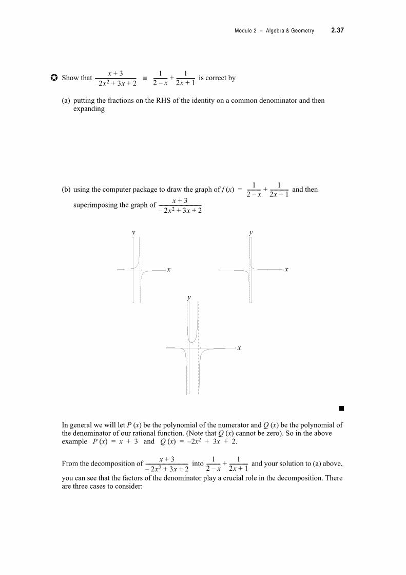
Show that is correct by
(a) putting the fractions on the RHS of the identity on a common denominator and then expanding
(b) using the computer package to draw the graph of f (x) = and then
superimposing the graph of
■
In general we will let P (x) be the polynomial of the numerator and Q (x) be the polynomial of the denominator of our rational function. (Note that Q (x) cannot be zero). So in the above example P (x) = x + 3 and Q (x) = –2x2 + 3x + 2.
From the decomposition of into and your solution to (a) above,
you can see that the factors of the denominator play a crucial role in the decomposition. There are three cases to consider:
x 3+
2x2 3x 2+ +–---------------------------------
1
2 x–-----------
1
2x 1+---------------+*
1
2 x–-----------
1
2x 1+---------------+
x 3+
2x2– 3x 2+ +----------------------------------
x
y
x
y
x
y
x 3+
2x2– 3x 2+ +----------------------------------
1
2 x–-----------
1
2x 1+---------------+

2.38 TPP7184 – Mathematics Tertiary Preparation Level D
1. If Q (x) can only be expressed as the product of linear factors then the partial fractions will have numerators that are numbers.
e.g.
If Q (x) can only be expressed as the product of a linear factor and an irreducible quadratic factor then the partial fraction with the linear factor of Q (x) as the denominator will have a number as the numerator, and the partial fraction with the irreducible quadratic factor of Q (x) as the denominator will have a numerator which is a polynomial of degree 1. See Note 1
e.g.
If Q (x) has repeated factors then we must include a partial fraction for each power of the repeated factor.
e.g.
e.g.
Notes
1. An irreducible quadratic is one which cannot be factorised into linear factors eg x2 + 1 = 0.
x 3+
2x2– 3x 2+ +----------------------------------
x 3+
2 x–$ % 2x 1+$ %-------------------------------------
1
2 x–-----------
1
2x 1+---------------+= =
numbers
two different linear factors
4x2 7x 3+–
x3 2x2 x– 2+ +----------------------------------------
4x2 7x– 3+
2 x–$ % 1 x2+$ %------------------------------------
1
2 x–-----------
1 3x–
1 x2+------------------+= =
+ , -
number
polynomial of degree 1
linear factor
irreducible quadratic factor
1
x3 2x2– x+----------------------------
1
x x 1–$ % x 1–$ %$ %-----------------------------------------
1
x---
1–
x 1–$ %------------------
1
x 1–$ %2------------------------------+ += =
. / / 0 / / 1 . 0 1 . / 0 / 1
(x – 1) is repeated twice and (x – 1) is linear
1st power of (x – 1)
2nd power of (x – 1)
x3 1–
x4 8x2 16+ +--------------------------------
x3 1–
x2 4+$ % x2 4+$ %------------------------------------------
x
x2 4+------------------
4x– 1–
x2 4+$ %2------------------------------+= =
. / / 0 / / 1
2. 0 1
+ / , / -
. / 0 / 1
(x2 + 4) is repeated twice and (x2 + 4) is an irreducible quadratic
1st power of (x2 + 4)
2nd power of (x2 + 4)
polynomials of degree 1

Module 2 – Algebra & Geometry 2.39
The procedure for the decomposition of rational functions into partial fractions is as follows.
Step 1: Factorise the denominator Q (x) into a product consisting of linear factors and/or quadratic factors.
Note if any factor is repeated.
Step 2: Write the numerators of the partial fractions in general terms and form an identity.
Step 3: Clear fractions from each side of the identity; expand brackets; simplify.
Step 4: Equate coefficients of each power of x on each side of the identity. (This is valid because the mathematical statement is an identity.)
Step 5: Solve for constants.
Step 6: Substitute for unknowns in original partial fractions.
Step 7: Check that the partial fractions when placed on a common denominator and ‘tidied-up’ yield the original rational function.
Example 2.9: Decompose into partial fractions.
Step 1: Check that P (x) and Q (x) are indeed polynomials and that P(x) does not have higher degree than Q (x)). As this is the case factorise the denominator. You can do this factorisation by inspection or by using the quadratic formula.
Q (x) = –2x2 + 3x + 2 = (2 – x) (2x + 1)
Therefore we have the product of two non-identical linear factors.
Step 2: where A and
B are the numbers to be determined.
Step 3:
Clear fractions on RHS by multiplying through by (2 – x) (2x + 1) (i.e. put rational functions on RHS on a common denominator)
x + 3 = A (2x + 1) + B (2 – x)
Expanding brackets on RHS
x + 3 = 2Ax + A + 2B – Bx
x 3+
2x2 3x 2+ +–---------------------------------
P x$ %Q x$ %------------
x 3+
2x2– 3x 2+ +----------------------------------
x 3+
2 x–$ % 2x 1+$ %-------------------------------------
A
2 x–$ %----------------
B
2x 1+$ %--------------------+*= =
x 3+
2 x–$ % 2x 1+$ %-------------------------------------
A
2 x–$ %----------------
B
2x 1+$ %--------------------+*
x 3+
2 x–$ % 2x 1+$ %------------------------------------- 2 x–$ % 2x 1+$ %"
A
2 x–$ %---------------- 2 x–$ % 2x 1+$ %"
B
2x 1+$ %--------------------+ 2 x–$ % 2x 1+$ %"=
2.40 TPP7184 – Mathematics Tertiary Preparation Level D
Gathering terms with same powers of x together
x + 3 =
x + 3 = (2A – B) x +
Step 4: Equating coefficients of each power of x on each side of the identity
Coefficient of x1 on LHS is 1; coefficient of x1 on RHS is (2A – B)
1 = 2A – B
Coefficient of x0 (i.e. the value of the constant) on LHS is 3; coefficient of x0 on RHS is (A + 2B)
3 = A + 2B
Step 5: Solving simultaneously for A and B in
1 = 2A – B3 = A + 2B
yields A = 1 and B = 1
Step 6:
Step 7: Check solution
=
=
=
=
= which is the original rational function ✓
This is not a very easy section of work but it is important later on for calculus. Work carefully through the next examples filling in the blanks and the boxes. As you gain confidence you will be able to omit some steps.
2Ax Bx–$ % A 2B+$ %+
A 2B+$ %
x 3+
2 x–$ % 2x 1+$ %-------------------------------------
A
2 x–-----------
B
2x 1+--------------- =+
1
2 x–-----------
1
2x 1+---------------+*
1
2 x–-----------
1
2x 1+---------------+
1 2x 1+$ % 1 2 x–$ %+
2 x–$ % 2x 1+$ %-------------------------------------------------
2x 1 2 x–+ +
2 x–$ % 2x 1+$ %-------------------------------------
x 3+
2 x–$ % 2x 1+$ %-------------------------------------
x 3+
4x 2 2x2– x–+--------------------------------------
x 3+
2x2– 3x 2+ +----------------------------------

Module 2 – Algebra & Geometry 2.41
Example 2.10: Complete the decomposition of into partial fractions
Solution:
Step 1: Denominator, Q(x) is See Note 1
Through trial and error and intelligent guessing I find (2 – x) is a factor of
–x3 + 2x2 – x + 2.
Use long division to find other factor.
Q (x) = –x3 + 2x2 – x + 2 = (2 – x) (...........................)
Note no repeated factors but second factor is an .................................... quadratic
Step 2:
where A, B and C are to be determined
Step 3: Multiply through by (2 – x) (1 + x2) to clear fractions
4x2 – 7x + 3 = A " ( ..................... ) + (Bx + C) ( ....................... )
Expanding brackets on RHS
4x2 – 7x + 3 = A + Ax2 + 2Bx – Bx2 + 2C – Cx
Gathering terms with same powers of x together
4x2 – 7x + 3 = ( ) x2 + ( ) x + (A + 2C)
Notes
1. A negative coefficient for x3 indicates that at least one factor as a –x term.
4x2 7x– 3+
x3– 2x2 x– 2+ +------------------------------------------
–x3 + 2x2 – x + 2
x3– 2x2 x– 2+ +2 – x
P x$ %Q x$ %------------
4x2 7x– 3+
x3– 2x2 x– 2+ +------------------------------------------
4x2 7x– 3+
2 x–$ % 1 x2+$ %------------------------------------
A
2 x–-----------
Bx C+
1 x2+------------------+*= =
+ , -
polynomial of degree 1
4x2 7x– 3+
2 x–$ % 1 x2+$ %------------------------------------ 2 x–$ % 1 x2+$ %"
A
2 x–$ %---------------- 2 x–$ % 1 x2+$ %"
Bx C+$ %1 x2+
--------------------- 2 x–$ % 1 x2+$ %"+=

2.42 TPP7184 – Mathematics Tertiary Preparation Level D
Step 4: Coefficient of x2 on LHS is ; coefficient of x2 on RHS is (A – B)
Coefficient of x1 on LHS is ; coefficient of x1 on RHS is (2B – C)
Coefficient of x0 on LHS is ; coefficient of x0 on RHS is (A + 2C)
Step 5: Equating coefficients of powers of x yields
4 = A – B–7 = 2B – C Solution of these three euqations is shown on page 2.45
3 = A + 2C
Solving simultaneously gives
A = ; B = ; C =
Step 6:
Step 7: Check solution
=
=
=
=
= ✓
Example 2.11: Complete the decomposition of into partial fractions
Solution:
Step 1: Q(x) = x3 – 2x2 + x = x ( ) ( )
Note (x – 1) is repeated ............................. and (x – 1) is a .......................... factor
Step 2:
4x2 7x– 3+
2 x–$ % 1 x2+$ %------------------------------------
A
2 x–-----------
Bx C+
1 x2+-----------------+*
1
2 x–$ %----------------
3x– 1+
1 x2+$ %-------------------+=
1
2 x–-----------
3x– 1+
1 x2+-------------------+
1$ % 3x– 1+$ %$ %+
2 x–$ % 1 x2+$ %------------------------------------------------------------------------------------
2 x–$ % 1 x2+$ %----------------------------------------------------------------------
4x2 7x– 3+
2 x–$ % 1 x2+$ %------------------------------------
4x2 7x– 3+----------------------------------------------------------------------
4x2 7x– 3+
x3– 2x2 x– 2+ +------------------------------------------
1
x3 2x2– x+----------------------------
1
x3 2x2 x+–----------------------------
1
x x 1–$ %2----------------------
A
x----
B
x 1–$ %----------------
C----------------+ +*=

Module 2 – Algebra & Geometry 2.43
Step 3:
1 = A(x – 1)2 + Bx(x – 1) + Cx= A(x2 – 2x + 1) + Bx(x – 1) + Cx= Ax2 – 2Ax + A + Bx2 – Bx + Cx
1 = ( ) x2 + ( ) x + (A)
Step 4: Coefficient of x2 on LHS is 0; coefficient of x2 on RHS is (A + B)
Coefficient of x1 on LHS is ; coefficient of x1 on RHS is
Coefficient of on LHS is ; coefficient of x0 on RHS is (A)
Step 5: 0 = A + B
0 = –2A – B + C
1 =
Solving simultaneously (not shown here) yields
A = ; B = ; C =
Step 6:
Step 7: Check solution
=
=
= ✓
1
x x 1–$ %2---------------------- x x 1–$ %2"
A
x---- x x 1–$ %2"
B
x 1–$ %---------------- x x 1–$ %2"
C
x 1–$ %2------------------- x x 1–$ %2"+ +=
1
x3 2x2 x+–----------------------------
A
x----
B
x 1–-----------
C
x 1–$ %2-------------------+ +*
x-------------------
1–-------------------
x 1–$ %2-------------------+ +=
1
x---
1–
x 1–$ %----------------
1
x 1–$ %2-------------------+ +
x x 1–$ %2-----------------------------------------------------------------------------------
x3 2x2 2x x2 x 1–+–+–-----------------------------------------------------------------------------------
1
x3 2x2 x+–----------------------------
2.44 TPP7184 – Mathematics Tertiary Preparation Level D
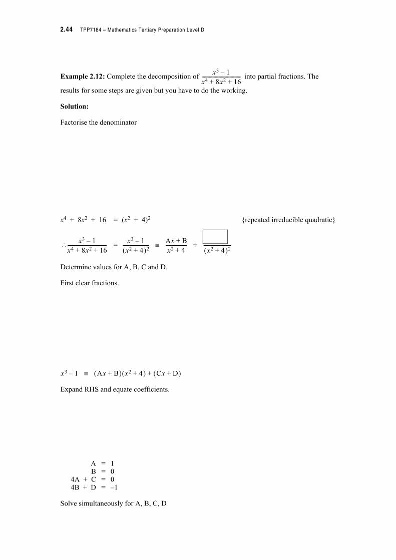
Example 2.12: Complete the decomposition of into partial fractions. The
results for some steps are given but you have to do the working.
Solution:
Factorise the denominator
x4 + 8x2 + 16 = (x2 + 4)2 {repeated irreducible quadratic}
=
Determine values for A, B, C and D.
First clear fractions.
Expand RHS and equate coefficients.
A = 1B = 0
4A + C = 04B + D = –1
Solve simultaneously for A, B, C, D
x3 1–
x4 8x2 16+ +--------------------------------
x3 1–
x4 8x2 16+ +--------------------------------
x3 1–
x2 4+$ %2---------------------
Ax B+
x2 4+-----------------
x2 4+$ %2-----------------------+*
x3 1 Ax B+$ % x2 4+$ % Cx D+$ %+*–

Module 2 – Algebra & Geometry 2.45
A = 1; B = 0; C = –4; D = –1
Check solution.
If you had difficulty with solving the little equations to obtain A, B, C etc. work through this next section otherwise if you now feel comfortable with the method for partial fractions try the following exercises.Solving several simultaneous equations involving more than two variables involves reducing the equations by various substitutions until two equations in the same two unknowns are obtained.
e.g. from Example 2.11
4 = A – B _________ !
–7 = 2B – C _________
3 = A+ 2C _________ !
From ", A = 4 + B
Substituting in ! for A yields
3 = 4 + B + 2C
–1 = B + 2C _________ #
Now and # are two equations in the same two unknowns.
From , C = 2B + 7
Substituting in # for C yields
–1 = B + 2 ! (2B + 7)
–15 = 5B B = –3
Substituting in C = 2B + 7 for B yields
C = 2 ! (–3) + 7 C = 1
Substituting in A = 4 + B for B yields
A = 4 + (–3) A = 1
x3 1–
x4 8x2 16+ +--------------------------------
1
x2 4+--------------
4x– 1–
x2 4+" #2---------------------+=

2.46 TPP7184 – Mathematics Tertiary Preparation Level D
Exercise Set 2.14
Express each of the following as partial fractions
• Take care that the numerator and denominator are both polynomials before attempting the decomposition.
• Also ensure that the numerator does not have a higher degree than the denominator. (If this is the case you will need to use long division to get the remainder as a proper rational function which you can then decompose into partial fractions.)
• Make sure you check your answers.
1.
2.
3.
4.
5.
6. (a)
(b) Using the result from 6(a) find and deduce the value of S$.
3 x–
2 x–" # 2x 1–" #------------------------------------
9x 72–
x3 3x2 18x––----------------------------------
x2 3x– 12+
2 x–" # 1 x2+" #------------------------------------
x3 2x2 x– 3+ +
x2 x– 6–--------------------------------------
9x
1 x+" # 1 2x–" #2---------------------------------------
1
r r 1+" #-------------------
Sn
r 1=
n
%1
r r 1+" #-------------------=
Module 2 – Algebra & Geometry 2.47
Other Important Non Linear Functions
In the last section of work you drew some graphs of rational functions. These make up one group of non linear functions that you need to be familiar with. (I’m assuming now you can draw polynomials easily.) In previous mathematics units you will have met many other non linear functions so here we will only briefly review the more important ones.
circles; and hyperbolas
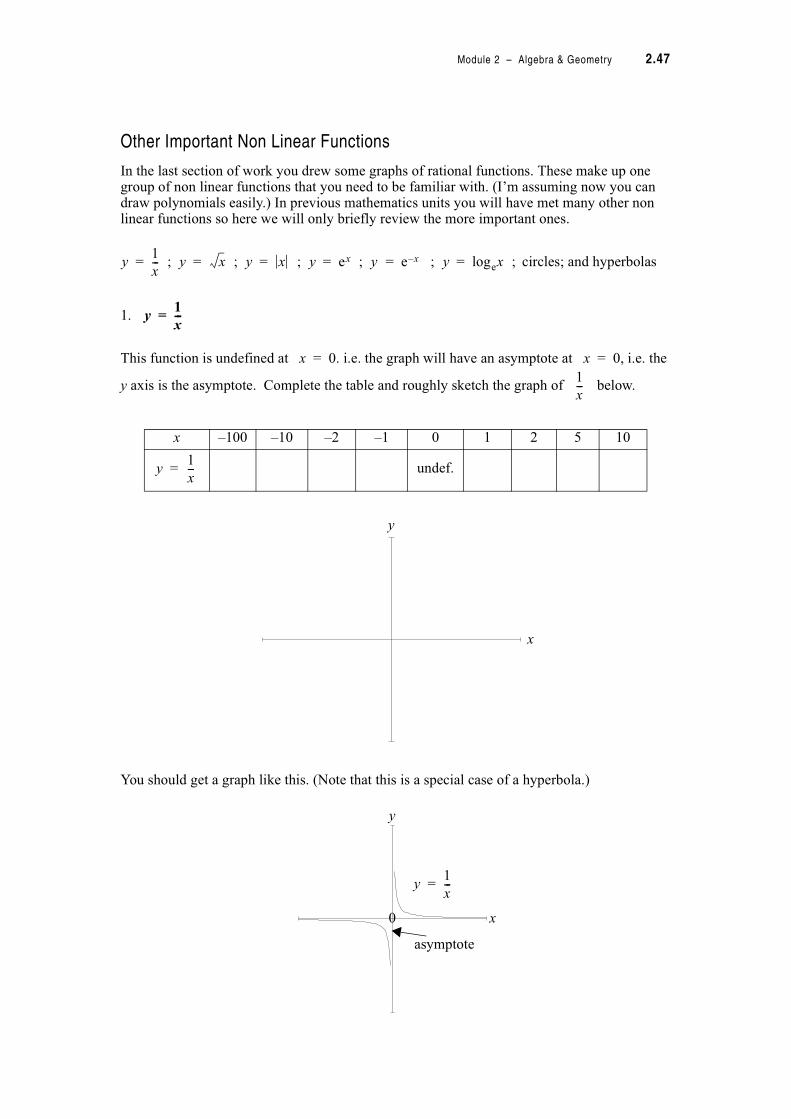
1.
This function is undefined at x = 0. i.e. the graph will have an asymptote at x = 0, i.e. the
y axis is the asymptote. Complete the table and roughly sketch the graph of below.
You should get a graph like this. (Note that this is a special case of a hyperbola.)
x –100 –10 –2 –1 0 1 2 5 10
y = undef.
y1
x--- ; y x ; y x ; y ex ; y = e x– ; y logex ;= = = = =
y1
x---=
1
x---
1
x---
y
x
y
x0
asymptote
y1
x---=
2.48 TPP7184 – Mathematics Tertiary Preparation Level D
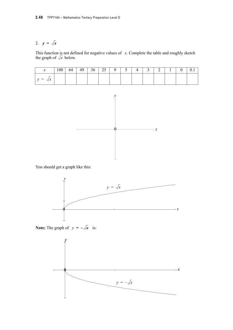
2.
This function is not defined for negative values of x. Complete the table and roughly sketch the graph of below.
You should get a graph like this:
Note: The graph of y = – is:
x 100 64 49 36 25 9 5 4 3 2 1 0 0.1
y =
y x=
x
x
y
x0
x
y
O0
y x=
y
x
x
x
y
O0y x–=
x
y

Module 2 – Algebra & Geometry 2.49
3.
This function is defined for all values of x. The output of the function is always positive because the symbol ‘ ’ means ‘absolute value’. Complete the table and roughly sketch the graph of below.
You should get a graph like this:
x –100 –50 –10 –5 –2 –1 0 1 2 5 10 50 100
y =
y x=
x
x
y
x0
xO
yy
x0
y x=

2.50 TPP7184 – Mathematics Tertiary Preparation Level D
4. y = ex
This is THE positive exponential function. i.e. the positive exponential function with base e. Complete the table and roughly sketch the graph of ex below. See Note 1
You should get a graph like this:
Notes
1. Exponential functions can have any base. The most common are e and 10.
x –100 –50 –10 –5 –2 –1 0 1 2 5 10 50 100
y = ex
y
x0
y
y = ex
1
0 x

Module 2 – Algebra & Geometry 2.51
5. y = e–x
This is THE negative exponential function. Complete the table and roughly sketch the graph of e–x below.
You should get a graph like this:
x –100 –50 –10 –5 –2 –1 0 1 2 5 10 50 100
y = e–x
y
x0
y
10 x
y ex–
=

2.52 TPP7184 – Mathematics Tertiary Preparation Level D
6. y = logex or ln x
This is the logarithmic function with base e. As for exponentials, logarithmic functions can have any base. The most common are e and 10. Use your calculator and roughly sketch the graph of y = ln x below.
You should get a graph like this:
Note: Do not confuse the graph of ln x and the graph of .
y
x0
y
01
x
y = ln x
x

Module 2 – Algebra & Geometry 2.53
7. Circles e.g.
i.e.
This circle is centred at (–1, 2) and has radius 2.
Note: The General Form of a circle is where (h, k) is the centre and r the radius.
The graph of (x + 1)2 + (y – 2)2 = 4 is:
8. Hyperbolas e.g. y = – 3
This hyperbola has vertical asymptote at x = 2; See Note 1
has horizontal asymptote at y = –3; See Note 2
cuts x-axis at ; and cuts y-axis at
Note: The General Form of an hyperbola is ,
where the vertical asymptote is at x = a;
horizontal asymptote is at y = b;
curve cuts x-axis at ;
Notes
1. When x & 2, y tends to +$ or –$ depending on whether x approaches 2 from the positive or negative
side. Under such conditions we say the function has a vertical asymptote at x = 2.
2. As x & +$ or –$, y tends to –3, thus the function has a horizontal asymptote at y = –3.
x 1+" #2 y 2–" #2+ 4=
x 1+" #2 y 2–" #2+ 22=
x h–" #2 y k–" #2+ r2=
1
x 2–-----------
7
3---, 0' () * 0,
7–
2------' (
) *
yc
x a–------------ b+=
ac
b---, 0–' (
) *

2.54 TPP7184 – Mathematics Tertiary Preparation Level D
curve cuts y-axis at
This is the form of the hyperbola that we will use in this unit. In your previous studies (e.g. in unit 11083) you may have met an alternative form of the hyperbola based on a geometric
construction of this type of function when it is centred at the origin. e.g. where
b2 = c2 – a2 and the hyperbola has foci at (–c, 0) and (c, 0).
Complete the table and draw the graph of y = – 3 below.
x –2 –1 0 1 2 3
0, bc
a--–' (
) *
x2
a2-----
y2
b2-----– 1=
1
x 2–-----------
y1
x 2–----------- 3–=
y
x0
Module 2 – Algebra & Geometry 2.55
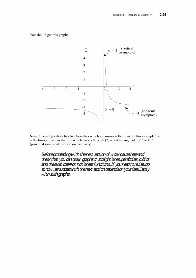
You should get this graph:
Note: Every hyperbola has two branches which are mirror reflections. In this example the reflections are across the line which passes through (2, –3) at an angle of 135+ or 45+ (provided same scale is used on each axis)
Before proceeding with the next section of work pause here and check that you can draw graphs of straight lines, parabolas, cubics and the most common non linear functions. If you need to revise, do so now, as success with the next section depends on your familiarity with such graphs.
–4 –3 –2 –1 2 3 4
yx = 2
(vertical asymptote)
x
(2, –3)y = –3
(horizontal asymptote)
4
3
2
1
–1
–2
–3
–4

2.56 TPP7184 – Mathematics Tertiary Preparation Level D
Solving Simultaneous Equations Algebraically and Graphically
Solving simple simultaneous algebraic equations is easy if the equations are linear.
Example 2.13: Solve y = 2x + 7y = –2x + 5
Solution:
This set of equations can be solved algebraically by
(i) equating the two Right Hand Sides; solving for x; substituting to get y, or
(ii) by adding the two equations (thus eliminating x) and solving for y; substituting to getx.
Method (i) Method (ii)
2x + 7 = –2x + 5 2y = 12
4x = –2 y = 6
x = – y = 2x + 7
y = 2x + 7 6 = 2x + 7
= 2 ! – + 7 x = – & Point (– , 6)
= 6 & Point (– , 6)
(– , 6) satisfies both equations and hence is the required solution.
The set of equations can also be solved graphically. Solving these equations graphically means we are looking for points where the graphs of the equations intersect.
1
2---
1
2---
1
2---
1
2---
1
2---
1
2---
y
y = 2x + 7
y = –2x + 5
(–1, 2, 6)
x
. 6
½–3½ 2½

Module 2 – Algebra & Geometry 2.57
Example 2.14: Solve y = 3x + 2 _________"x2 + y2 = 4 _________
Solution:
Algebraically:
From ", y = 3x + 2 substitute in for y
x2 + (3x + 2)2 = 4
x2 + 9x2 + 12x + 4 = 4
10x2 + 12x = 0
x(10x + 12) = 0
x = 0 or x = –
From ", when x = 0, y = 3 ! 0 + 2 = 2 & (0, 2) as one solution
From ", when x = – , y = 3 ! – + 2 = – & (– , – ) as the other solution
There are two solutions: when x = 0, y = 2 and
when x = – , y = –
Graphically:
To solve these equations graphically, examine the equations and determine the types of graphs involved.
y = 3x + 2 is a straight line with slope 3 and y-intercept of 2 ; and x2 + y2 = 4 is a circle with centre at (0, 0) and radius 2.
Drawing the graphs of these equations gives:
and zooming in on the points of intersection yields the required solutions of (0, 2) and (– , – )
Whenever possible we solve equations algebraically as then the solution is exact. If we cannot do this (or it is computationally difficult) graphical techniques are often used.
6
5---
6
5---
6
5---
8
5---
6
5---
8
5---
6
5---
8
5---
Check solutions by
substituting in both
original equations-./.0
6
5---
8
5---

2.58 TPP7184 – Mathematics Tertiary Preparation Level D
Example 2.15: Solve .
Solution:
We can write this equation as .
If we let and , then, when y1 = y2 (i.e. ) we have the solution of the original equation.
To solve this set of equations is quite messy but it is easy to do graphically.
y1 = x2 – 3 is a parabola, saucer shaped (i.e. with a minimum) which cuts the y-axis at
y = 3. Its axis of symmetry is x = . Following the work in the Revision Module or using
calculus (if you have studied course TPP7183 / 11083 or its equivalent) you can draw
y1 = x2 – 3.
y2 = is a non linear equation whose graph we also know and can therefore draw.
We are interested only in those parts of the graphs where the curves intersect. A rough sketch shows that the curves intersect once only, at about (2.1, 1.5). To obtain a better estimate you can redraw the curves for the domain say from x = 1 to x = 3 or zoom in on the point of intersection using your computer package.
Now you can use the graphical technique to solve simultaneous equations you have a tool for finding roots of and solving quite complicated equations. Here’s one more example before you try the exercise set.
x2 3– x– 0=
x2 3– x=
y1 x2 3–= y2 x= x2 3– x=
3
2---
x
−4 −2 0 2 4 6
−4
−2
0
2
4
6
−4 −2 0 2 4 6
−4
−2
0
2
4
6
y1 = x2 – 3
approx. (2.1, 1.5)
y2 x=
y
x

Module 2 – Algebra & Geometry 2.59
Example 2.16: Find the positive solution of x + 3 = e0.5x
Solution:
The solutions of x + 3 = e0.5x are the same values of x which satisfy the simultaneous equations,
y1 = x + 3y2 = e0.5x
Using the graphical approach seems sensible.
So the positive solution is x 3.8. We can check the validity of this solution by substituting in the original equation.
x + 3 = e0.5x
Consider LHS: when x = 3.8x + 3 = 3.8 + 3 = 6.8
Consider RHS: when x = 3.8e0.5x = e0.5 3.8 = e1.9 = 6.69 6.8
So x = 3.8 is a reasonable approximation to the solution.
Using your computer package you could zoom in on the point of interest and obtain a more accurate approximation.
−4 −2 0 2 4 6
−2
0
2
4
6
8
10
12
14
−4 −2 0 2 4 6
−2
0
2
4
6
8
10
12
14y
y2 = e0.5x
y1 = x + 3
x ! 3.8
We want the positive solution
negative solution
x
!
!

2.60 TPP7184 – Mathematics Tertiary Preparation Level D
Exercise Set 2.15
For Questions 1–8 find the solution of each of set of simultaneous equations. Use your graphing package where appropriate.
1. y = 2x + 4y = 8x – 2
2. y = 2x – 4y = 2x + 6
3. (x – 2)2 + (y – 4)2 = 16x = 3
4. x2 + y2 = 1(x – 3)2 + y2 = 4
5. x2 + y2 – 4x + 2y + 4 = 0 [Hint: Complete the square for x and for y to obtain y = –3x the standard form of a circle for the first equation.]
6. The equation of the circle passing through (0, 0), (0, 3) and (1, 0)y = ln x [Hint: Write three equations to the circle using each of the
coordinates given and then solve to get h, k and r]
7. y = e–x [Hint: Multiply numerator and denominator of by –1 to
y = + 2 for x < 1 get the second equation in standard form of a hyperbola.]
8. y =
y =
9. Obtain an approximate value for the positive solution of the equation(x + 1) (2 – x) = 5 ln (1 + x) [Hint: Find the solution of y1 = (x + 1) (2 – x)
y2 = 5 ln (1 + x)]
3
1 x–-----------
3
1 x–-----------
2x
2
x---

Module 2 – Algebra & Geometry 2.61
Inverse Functions
In the Revision Module we said that a function defines the relationship between two sets.
e.g. the function b = b (a) = 3a says that b depends on the chosen value of a , and the value of b is given by three times the value of a.
Some ordered pairs given by this function are (2, 6), (4, 12), (8, 24) (100, 300), (–14, –42),
(0.2, 0.6) (– , – ) etc.
We also said that
• if an element in the domain x, maps to more than one element in the range y, then the relationship between x and y is not a function e.g. and x2 + y2 = 1 are not functions Graphically this means that at least one vertical line intersects the graph of the set of ordered pairs (x, y) at more than one point.
• a one-to-one function occurs when each element in the domain is paired with only one unique element in the range. y = 3x and y = are both one-to-one functions Graphically this means that horizontal lines will intersect with the graph of the function once only.
• a many-to-one function is one where different elements in the domain yield the same element in the range e.g. y = x2 is a many-to-one function because, for example, when x = 2 and when x = –2, the corresponding y values are both 4. Graphically this means that at least one horizontal line will intersect with the graph of the function in more than one place.
In this section we will examine how to find the inverse functional relationship i.e. the relationship which maps from the range to the domain, given that we know the relationship that maps from the domain to the range.
A function will have an inverse if each element of the domain is related to a unique element in the range i.e. if there is a one-to-one mapping from Set X to Set Y.
We will use the one-to-one function y = f (x) = 3x for –2 " x " 2 to demonstrate.
See Note 1
Notes
1. Only the integer values are shown but all the real numbers between –2 and 2 are in the Set X and hence all the real
numbers between –6 and 6 are in the Set Y.
1
8---
3
8---
y x#=
x
2–
1–
0
1
2$ %& '& '& '& '& '& '( ) 6–
3–
0
3
6$ %& '& '& '& '& '& '( )
Set X Set Y
3 times

2.62 TPP7184 – Mathematics Tertiary Preparation Level D
If f is a one-to-one function and y = f (x), the inverse of f, denoted by f –1, is a unique function such that f –1 (f (x)) = x. See Note 1
So the inverse function has a domain which is the same as the range of the original function and a range which is the same as the domain of the original function.
For our example,
f (x) = 3x
So f –1 (x) has domain of –6 " x " 6 and range of –2 " y " 2.
What do you think is the functional relationship for f –1? [Hint: Examine the ordered pairs(x, y) with the order reversed.]
.....................................................................................................................................................
Answer:
You should have found that f –1 (x) = x.
The graphs of f (x) and f –1 (x) are shown here on the same set of axes.
Notes
1. f–1 (f(x)) is a composite function. In composite functions the output from the inner function becomes the input for the
outer function, e.g. if y = 2x and w = x2 + 1, (y(w(x)) is a composite function where the output from w(x) is the input
for y, e.g. if x = 3, y(w(x)) = 2(32 + 1) = 2 10 = 20.
2–
1–
0
1
2$ %& '& '& '& '& '& '( ) 6–
3–
0
3
6$ %& '& '& '& '& '& '( )
Domain of f Range of f
3 times
–2 " x " 2 –6 " y " 6
1
3---
−4 −2 0 2 4 6
−6
−4
−2
0
2
4
6
8
10
12
14
16
18
−4 −2 0 2 4 6
−6
−4
−2
0
2
4
6
8
10
12
14
16
18
y
f(x) = 3x
f 1– x* +1
3---x=
x

Module 2 – Algebra & Geometry 2.63
Now you can check that f –1 (f (x)) = x. Take any value for x, say x = 1.5, and read off the corresponding f (x) value. When x = 1.5, f (x) = f (1.5) = 4.5.
Now use that value of f (x) as the input value for f –1 (x).
When x = 4.5, f –1 (x) = f –1 (4.5) = 1.5, which was the original value chosen for x.
Try to show that f (f –1 (x)) = x also, by choosing a value of x, say x = 6, as the input for f –1 (x) first.
.....................................................................................................................................................
.....................................................................................................................................................
Answer:
From the graph when x = 6, reading from f –1 (x) we get, f –1 (6) = 2. Then when x= 2, reading from f(x) we get f(2) = 6
Redraw the graphs of f(x) = 3x and f –1(x) on the same axes with the same scale on each axis. Then draw a line at 45, to the x-axis on the axes (i.e. draw y = x). Can you see that f (x) and f –1 (x) are mirror images of each other across this line? (i.e. f and f –1 are symmetric about the line y = x)
Here’s another graphical example of a function and its inverse. (Drawing lines perpendicular to y = x and measuring each side of this line assists in getting the correct graph for the inverse.)
y = x
f(x)x
y f –1(x)

2.64 TPP7184 – Mathematics Tertiary Preparation Level D
Exercise Set 2.16
1. Examine the graphs below and determine which graphs represent functions.
Of the graphs that represent functions which are one-to-one?
Of the functions that are one-to-one which pairs of graphs represent functions and their inverses?
2. If f (x) = 3x + 2 and f –1 (x) = (x – 2)
(i) sketch f (x) and f –1 (x) on the same axes with the same scales on each axis.
(ii) choose two values of x and show graphically that f ( f –1 (x)) = x
(iii) choose two other values of x and show graphically that f –1(f (x)) = x.
(a) (b) (c) (d)
(e) (f) (g) (h)
(i) (j) (k) (l)
(q) (r) (s) (t)
(m) (n) (o) (p)
(u) (v)
1
3---

Module 2 – Algebra & Geometry 2.65
We need to be able to find the formula for inverse functions algebraically. We have a clue for the method from the graphical work just completed.
Example 2.17:
Find the inverse of f (x) = 5x + 3, if it exists.
Solution: First check by asking
• Is f (x) a one-to-one function? ‘Yes, it is a one-to-one function as it is a straight line and any horizontal line will intersect with it once only.’
• Is the domain of f (x) restricted? ‘No, f (x) is defined for all values of x as there are no restrictions given.’
f (x) = 5x + 3i.e. y = 5x + 3
Now in f –1 (x) the variables x and y have opposite to roles to those in f (x).
[Recall the change in order of the ordered pairs of the mappings of Set X and Set Y.]
So we interchange the variables x and y to get
x = 5y + 3
and solve for y which will now be given by f –1
If x = 5y + 3
5y = x – 3
- y = (x – 3)
i.e. f –1 (x) = (x – 3)
As we usually do, we now try to validate our answer. If we can show that f –1 (f (x)) = x or f (f –1 (x)) = x, then our inverse must be correct.
✓
1
5---
1
5---
f f 1– x* +* + f 1
5--- x 3–* +$ %
( ) 51
5--- x 3–* +$ %
( ) 3+ x 3– 3+ x= = = =
. / 0 / 1 . / 0 / 1
output from f –1
which becomesinput for f
input for f

2.66 TPP7184 – Mathematics Tertiary Preparation Level D
Exercise 2.18:
Find the inverse of y = x2 – 2, if it exists.
Solution: First check
• Is f (x) a one-to-one function? ‘No, f (x) = x2 – 2 is a parabola and thus at least one horizontal line will cut its graph in more than one place. This means f is not a one-to-one function - its inverse does not exist.’
Example 2.19:
Find the inverse of y = x2 + x – 6, where x > – , if it exists.
Solution: First check
• Is f (x) a one-to-one function? ‘No it is not as it is a parabola, but the domain is
restricted to x > – - need to check if for this restricted domain f is one-to-one.’
The easiest way to do this is to sketch the graph of y = x2 + x – 6
1
2---
1
2---
The part of the graph we are interested in
(i.e. for x > – ) is shown by the heavier
line and we note that for this restricted domain f is indeed one-to-one.
Domain of f is – < x < 2
and Range of f is –6 < y < 2
- Domain of f –1 is –6 < x < 2
and Range of f –1 is – < y < 2
1
2---
1
2---
1
4---
1
4---
1
2---
y
x21–3
–2
Graph of f (x) = x2 + x – 6
axis ofsymmetry
x = –1
2---
1
2
3
4
5
6
–4
–6
–1–2

Module 2 – Algebra & Geometry 2.67
Now we will find f –1(x) algebraically.
If f (x) = x2 + x – 6 for – < x < 2
i.e. y = x2 + x – 6 for – < x < 2
Let x = y2 + y – 6
- y2 + y = 6 + x
- (y + )2 – = 6 + x {Completing the square for y on LHS.}
- (y + )2 = x + 6
y + =
- y = –
i.e. f –1 (x) = –
Check solution
f –1 (f (x)) =
=
=
= {Positive root only because of restricted domain}
=
= x ✓
■
We will meet inverse trigonometric functions in a later module. Other important functions that you need to be able to find and use inverses for are the exponential and logarithmic functions.
If f (x) = ax, f –1 (x) = logax.
So f (f –1 (x)) = = x and f –1 (f (x)) = logaax = x
e.g. If f (x) = ex, f –1 (x) = logex or ln x
e.g. If f (x) = log2x, f –1 (x) = 2x
1
2---
1
2---
1
2---
1
4---
1
2---
1
4---
1
2--- x 6
1
4---++
x 61
4---+
1
2---
x 61
4---+
1
2---
f 1– x2 x 6–+* +
. / 0 / 1output from f to be used as input for f–1
x2 x 6–+* + 61
4---+
1
2---–
x2 x1
4---+ +
1
2---–
x1
2---+$ %
( )2 1
2---–
x1
2---
1
2---–+
alogax

2.68 TPP7184 – Mathematics Tertiary Preparation Level D
Exercise Set 2.17
1. If f(x) equals the height in centimetres of a person who weighs x kilograms what is the meaning of f –1(100) in practical terms?
2. Decide if the function f will have an inverse for each of the following scenarios
(i) f(d) is the number of litres of petrol in your car tank when the odometer reads d km.
(ii) f(t) is the number of customers in your local store at t minutes past noon on January 8, 1996.
(iii) f(x) is the volume in litres of x kilograms of ice at 4,C.(iv) f(n) is the number of first year students whose birthday is on the nth day of the
year.(v) f(w) is the cost in cents of mailing a letter that weighs w grams.
3. Consider the table of values below
(i) will f(x) have an inverse? Explain your answer.(ii) if the domain of f(x) is the integers from 1 to 7, what is the domain and range of
f –1(x)?
4. Consider the function f(x) = x2 + 3x
(i) why does this function not have an inverse?(ii) choose a domain for f(x) so that the inverse can be found.(iii) sketch f(x) for this restricted domain and f –1(x) on the same axes.
5. The cost, C of producing P articles is given by the function
C(P) = 100 + 2P
(i) should the domain of C(P) be restricted? If so, how?(ii) find the formula for the inverse function.(iii) explain in practical terms what the inverse function tells you.
6. Find the inverse function for each of the following. Prove your solutions are correct.
(i) f(x) = 2 + 3x (iv) f(x) = 2x3 – 4
(ii) f(x) = 1 – x2 for x 3 0 (v) f(x) = 2x2–1 for x 3 0
(iii) f(x) = 50e0.1x
x 1 2 3 4 5 6 7
f(x) 3 –7 19 4 178 2 1
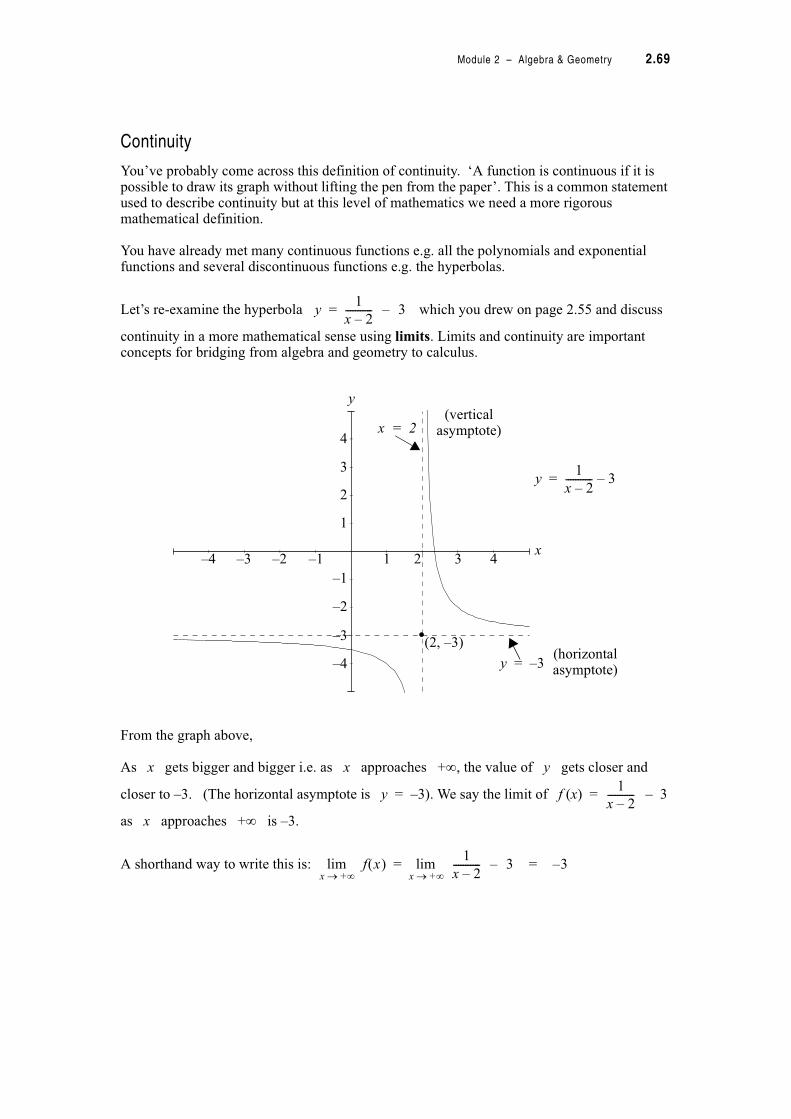
Module 2 – Algebra & Geometry 2.69
Continuity
You’ve probably come across this definition of continuity. ‘A function is continuous if it is possible to draw its graph without lifting the pen from the paper’. This is a common statement used to describe continuity but at this level of mathematics we need a more rigorous mathematical definition.
You have already met many continuous functions e.g. all the polynomials and exponential functions and several discontinuous functions e.g. the hyperbolas.
Let’s re-examine the hyperbola which you drew on page 2.55 and discuss
continuity in a more mathematical sense using limits. Limits and continuity are important concepts for bridging from algebra and geometry to calculus.
From the graph above,
As x gets bigger and bigger i.e. as x approaches +2, the value of y gets closer and
closer to –3. (The horizontal asymptote is y = –3). We say the limit of f (x) = – 3
as x approaches +2 is –3.
A shorthand way to write this is:
y1
x 2–----------- 3–=
–4 –3 –2 –1
–3
2 3 4x
y
x = 2(vertical
asymptote)
y1
x 2–----------- 3–=
(2, –3)
y = –3(horizontal asymptote)
1
4
3
2
1
–1
–2
–4
1
x 2–-----------
x +24lim f x !
x +"#lim
1
x 2–----------- 3– 3–= =
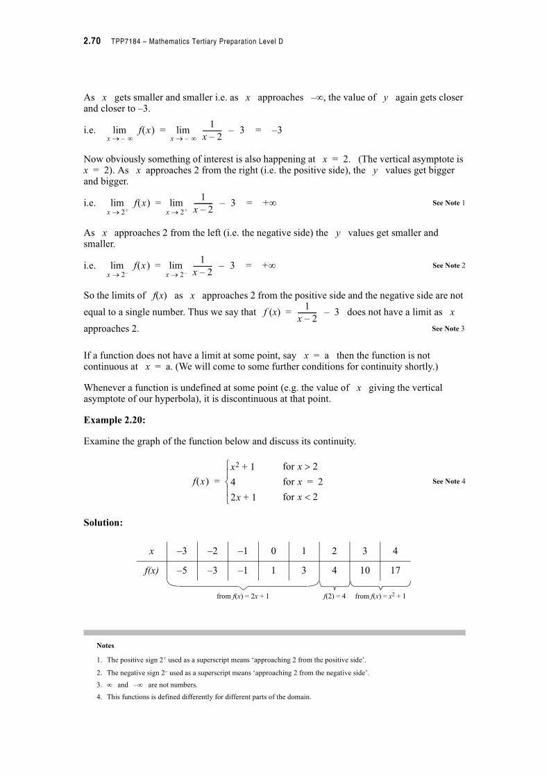
2.70 TPP7184 – Mathematics Tertiary Preparation Level D
As x gets smaller and smaller i.e. as x approaches –", the value of y again gets closer and closer to –3.
i.e.
Now obviously something of interest is also happening at x = 2. (The vertical asymptote is x = 2). As x approaches 2 from the right (i.e. the positive side), the y values get bigger and bigger.
i.e. See Note 1
As x approaches 2 from the left (i.e. the negative side) the y values get smaller and smaller.
i.e. See Note 2
So the limits of f(x) as x approaches 2 from the positive side and the negative side are not
equal to a single number. Thus we say that f (x) = – 3 does not have a limit as x
approaches 2. See Note 3
If a function does not have a limit at some point, say x = a then the function is not continuous at x = a. (We will come to some further conditions for continuity shortly.)
Whenever a function is undefined at some point (e.g. the value of x giving the vertical asymptote of our hyperbola), it is discontinuous at that point.
Example 2.20:
Examine the graph of the function below and discuss its continuity.
See Note 4
Solution:
Notes
1. The positive sign 2+ used as a superscript means ‘approaching 2 from the positive side’.
2. The negative sign 2– used as a superscript means ‘approaching 2 from the negative side’.
3. " and –" are not numbers.
4. This functions is defined differently for different parts of the domain.
x "–#lim f x !
x "–#lim
1
x 2–----------- 3– 3–= =
x 2+#lim f x !
x 2+#lim
1
x 2–----------- 3– +"= =
x 2–#lim f x !
x 2–#lim
1
x 2–----------- 3– +"= =
1
x 2–-----------
f x !
x2 1+
4
2x 1+$%&%'
=
for x 2(
for x 2=
for x 2)
x –3 –2 –1 0 1 2 3 4
f(x) –5 –3 –1 1 3 4 10 17
from f(x) = 2x + 1 f(2) = 4 from f(x) = x2 + 1

Module 2 – Algebra & Geometry 2.71
Something interesting is happening near x = 2. Let’s investigate the continuity of this function at x = 2
=
= 5
=
= 5
So as = , we can say that the exists and equals 5.
But is the graph continuous at x = 2?
Obviously no, because when x = 2 exactly, the value of the function is given as 4.
So the functional value at x = 2 does not equal the limit at x = 2.
So this provides us with the definition of continuity that you need to know for this level of mathematics.
−4 −2 0 2 4 6
−2
0
2
4
6
8
10
12
14
16
18
−4 −2 0 2 4 6
−2
0
2
4
6
8
10
12
14
16
18
−4 −2 0 2 4 6
−2
0
2
4
6
8
10
12
14
16
18
y
y = x2 + 1
open dot shows this point does not give the functional value when x = 2.
closed dot shows this point gives the functional value when x = 2.
(2, 4)
y = 2x + 1
x 2+#lim f x !
x 2+#lim x2 1+ (because x2 + 1 is the function for the
domain x greater than 2)
x 2–#lim f x !
x 2–#lim 2x 1+ (because 2x + 1 is the function for the
domain x less than 2)
x 2+#lim f x !
x 2–#lim f x ! 5=
x 2#lim f x !

2.72 TPP7184 – Mathematics Tertiary Preparation Level D
See Note 1
Make sure you understand these conditions.Example 2.21:
Discuss the limit and continuity of f (x) at x = 1 if
Solution:
= = 1
= = 1
* = 1
But the function is not defined at x = 1 * the function is not continuous at x = 1.See Note 2
A function f (x) is continuous at some point x = a iff these three conditions are met
1. = = single number
i.e. exists;
2. f (a) is defined; and
3. f (a) =
Notes
1. ‘Iff’ is read as ‘if and only if’.
2. Careful examination of the domain is required when several functions define f(x).
x a+#lim f x !
x a–#lim f x !
x a#lim f x !
x a#lim f x !
f x !1
x$&'
= for x 1(
for x 1)
x 1+#lim f x !
x 1+#lim 1
x 1–#lim f x !
x 1–#lim x
x 1#lim f x !

Module 2 – Algebra & Geometry 2.73
Exercise Set 2.18
1. Complete each table and use it to intuitively find the required limit.
(i)
(ii)
(iii)
(iv)
x –1.1 –1.01 –1.001 –0.999 –0.99 –0.9
f(x) = x2 – 2
x –0.2 –0.1 –0.01 0.01 0.1 0.2
x –2.5 –2.9 –2.99 –3.01 –3.1 –3.5
x (radian) –0.2 –0.1 –0.01 0.01 0.1 0.2
x – 1#lim x2 2– ! ?=
f x !x2 x+
x--------------=
x 0#lim
x2 x+
x-------------- ?=
f x !x2 9–
x 3+--------------=
x – 3#lim
x2 9–
x 3+-------------- ?=
f x !xtan
x--------------=
x 0#lim
xtan
x-------------- ?=
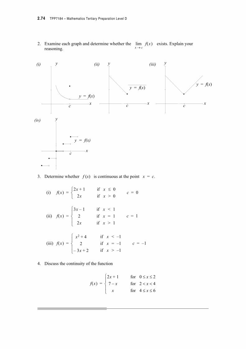
2.74 TPP7184 – Mathematics Tertiary Preparation Level D
2. Examine each graph and determine whether the exists. Explain your reasoning.
3. Determine whether f (x) is continuous at the point x = c.
(i)
(ii)
(iii)
4. Discuss the continuity of the function
x c#lim f x !
y
y = f(x)
xc
y
y = f(x)
cx
y
cx
y = f(x)
y
y = f(x)
x
(i) (ii) (iii)
(iv)
c
f x !2x 1+
2x$&'
=if x + 0
if x > 0c 0=
f x !
3x 1–
2
2x$%&%'
=
if x < 1
if x = 1
if x > 1
c 1=
f x !x2 4+
2
3x– 2+$%&%'
=
if x < –1
if x = –1
if x > –1
c 1–=
f x !
2x 1+
7 x–
x$%&%'
=
for 0 x 2+ +
for 2 x 4) )
for 4 x 6+ +

Module 2 – Algebra & Geometry 2.75
Solutions to Exercise Sets
Solutions Exercise Set 2.1 page 2.2
1. (a)
(b)
(c)
(d)
(e)
Solutions Exercise Set 2.2 page 2.4
1. x + 4 has the solution set ‘any real number less than or equal to 4’ or in intervalnotation, (–", 4]
e.g.
2. –2 < y has the solution set ‘any real number greater than –2’ or in interval notation(–2, ")
e.g.
3. + p + 3 has the solution set ‘any real number between and 3 and including
and 3’ or in interval notation
e.g.
1
4---– 0.25)
2– 3–(
,22
7------)
0.00012 1.2 10 4–-=
2.7 e)
180, 7, ,, 2, 2.41, ,, e, 10
3------, 2–––
1 000, 49.2, ,, e2, 2.111, 62
9---
1
2---–
1
2---–
1
2---–
1
2---– , 3
1
2---– , 0.499, 0.21,
1
5---– , 0, 1, 2, 2.48, 3––

2.76 TPP7184 – Mathematics Tertiary Preparation Level D
Solutions Exercise Set 2.3 page 2.7
1.
Check: Choose say See Note 1
and
✓
2.
*
* [Note the change in direction of the inequality]
* or
Check: Choose say
and
✓
3.
[Note the change in direction of the inequality]
Check: Choose say
and
✓
Notes
1. Choosing one particular value of x does not prove the solution is true but it does help in the checking process.
2x 4+ 8+
2x* 8 4–+
2x* 4+
* x 2 or ", 2]– +
x 1=
LHS 2x 4 2 1 4+-=+=* 6=
RHS 8 LHS RHS+*=
1
2---– p 2p 4+(
1
2---– p 2p 4(–
5
2---– p 4(
p 42–
5-------)
p8–
5------) ",
8–
5------–. /
0 1
x 3–=
LHS 1
2---– p
1
2---– 3–-=
3
2---= =*
RHS 2p 4 2 3– 4+- 2–= =+=
LHS RHS(*
2d 2+ 4d 3–+
2d 4d–* 3– 2–+
2d–* 5–+
d*5
2--- or
5
2---, "+ /
12
d 4=
LHS 2d 2 2 4 2 10=+-=+=*
RHS 4d 3 4 4 3 13=–-=–=
LHS RHS+*

Module 2 – Algebra & Geometry 2.77
Solutions Exercise Set 2.3 cont.
4. 3y – 2 2 4y + 6
* 3y – 4y 2 6 + 2
*
* [Note the change in direction of the inequality]
Check: Choose say
and
* ✓
5.
[Using the Distributive Law]
Check: Choose say
* ✓
6.
Absolute value of 2x + 4 is less than 3 means
2x + 4 < 3 and – (2x + 4) < 3
* 2x < –1 and * 2x – 4 < 3
* x < – and * –2x < 7
* x >
* < x < or
y 82–
y 8 or ", 8 3–– –+
y 10–=
LHS 3y 2– 3 10 2––-= = 32–=*
RHS 4y 6+ 4 10– 6+- 34–= = =
LHS RHS2
2y 3 y– ! 6 y– ! 3 2y+ !(
6y 2y2– 18 12y 3y– 2y2–+(
6y 2y2 12y– 3y 2y2+ +– 18(*
3y 18(–*
y 6–)* or ", 6–– !
y 7–=
LHS 2 7 3 7–– !–-=* 14 10-– 140–= =
RHS 6 7–– ! 3 2 7–-+ ! 13 11–- 143–= = =
LHS RHS(
2x 4+ 3)
1
2---
7–
2------
7
2---– '
1
2---–
7
2---
1
2---–4–. /
0 1
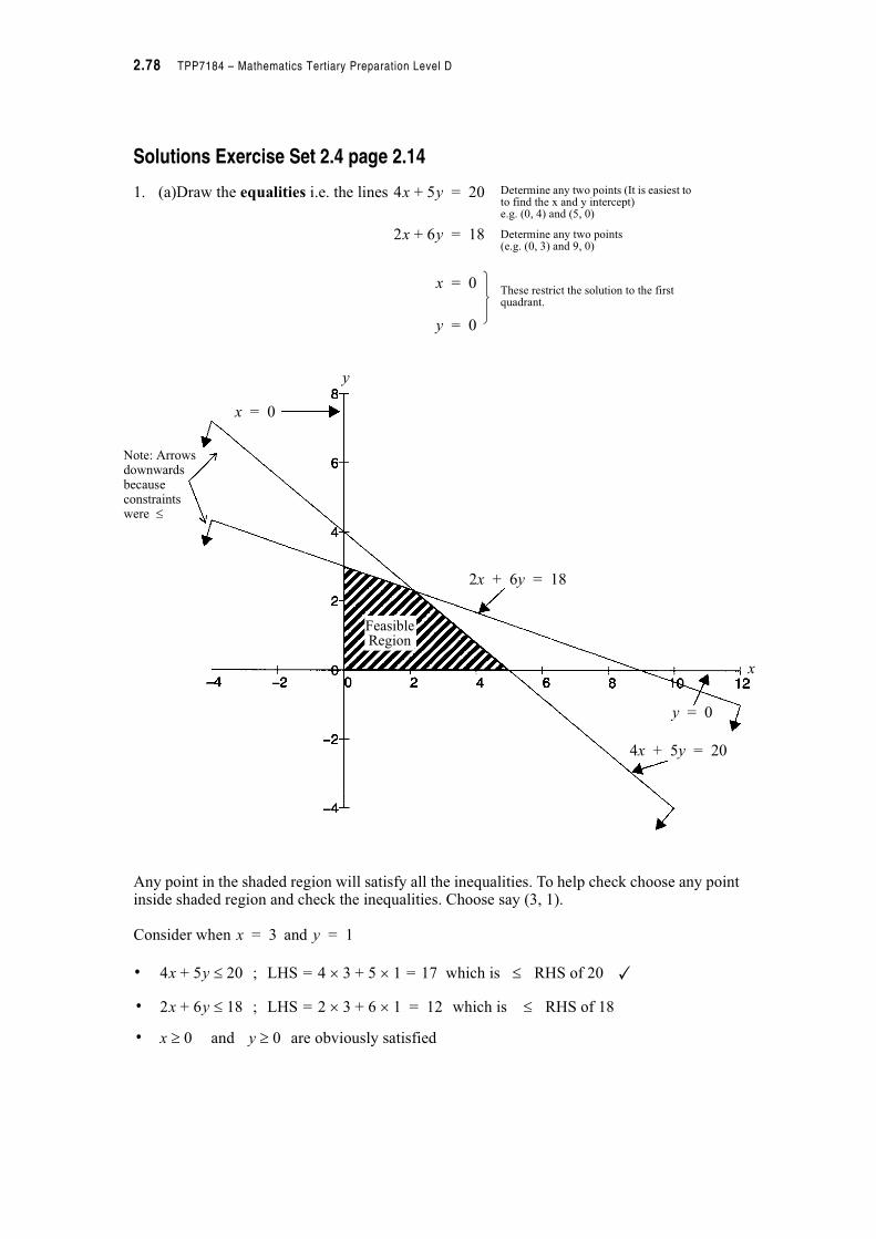
2.78 TPP7184 – Mathematics Tertiary Preparation Level D
Solutions Exercise Set 2.4 page 2.14
1. (a)Draw the equalities i.e. the lines
Any point in the shaded region will satisfy all the inequalities. To help check choose any point inside shaded region and check the inequalities. Choose say (3, 1).
Consider when and
• ✓
••
4x 5y+ 20=
2x 6y+ 18=
x 0=
y 0=
Determine any two points (It is easiest to to find the x and y intercept)e.g. (0, 4) and (5, 0)
Determine any two points(e.g. (0, 3) and 9, 0)
These restrict the solution to the first quadrant.
y
x
x = 0
2x + 6y = 18
y = 0
4x + 5y = 20
Feasible Region
Note: Arrowsdownwardsbecauseconstraintswere
x 3= y 1=
4x 5y 20 ; LHS 4 3 5 1!+! 17= =+ which is RHS of 20
2x 6y+ 18 ; LHS 2 3 6 1!+!= 12 which is RHS of 18 =
x 0 and y 0" are obviously satisfied"

Module 2 – Algebra & Geometry 2.79
Solutions Exercise Set 2.4 cont.
1. (b) The equalities are
Checking: Consider a point in the region, say (6, 4)
When and
• ✓
••
x y+ 6=
10x 2y+ 20=
y 2=
x 0=
Points for plotting: (0, 6), (6, 0)
(0, 10), (2, 0)
Care needs to be taken here# $
Note: Arrows upwards because constraints were "
y
x
FeasibleRegion
y = 2
x + y = 610x + 2y = 20
x = 0
x 6= y 4=
x y+ 6 ; LHS 6 4+ 10= =" which is RHS of 6"
10x 2y+ 20 ; LHS 10 6! 2 4 68=!+=" which is RHS of 20"
y 2 and x 0" are also satisfied"
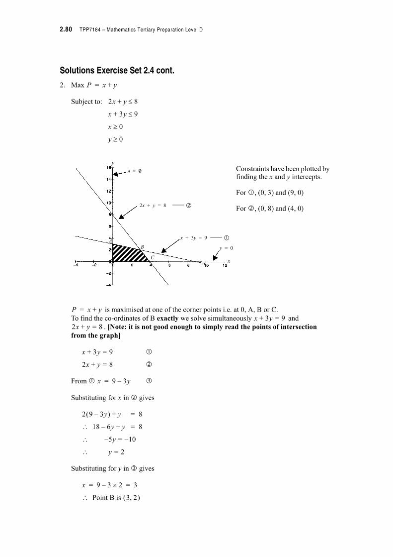
2.80 TPP7184 – Mathematics Tertiary Preparation Level D
Solutions Exercise Set 2.4 cont.
2. Max
Subject to:
is maximised at one of the corner points i.e. at 0, A, B or C.
To find the co-ordinates of B exactly we solve simultaneously and
. [Note: it is not good enough to simply read the points of intersection
from the graph]
!
From "
Substituting for x in ! gives
= 8
= 8
Substituting for y in " gives
P x y+=
2x y 8 +
x 3y 9 +
x 0"
y 0"
Constraints have been plotted by finding the x and y intercepts.
For , (0, 3) and (9, 0)
For !, (0, 8) and (4, 0)
x
y = 0
x + 3y = 9
C
BA
2x + y = 8 !
x = 0y
P x y+=
x 3y 9=+
2x y 8=+
x 3y 9=+
2x y 8=+
x 9 3y–=
2 9 3y–% & y+
18 6y–' y+
5y 10–=–'
y 2='
x 9 3 2!– 3= =
Point B is 3, 2% &'

Module 2 – Algebra & Geometry 2.81
Solutions Exercise Set 2.4 cont.
2. continued
Point Co Ord
0 (0, 0)
A (0, 3)
B (3, 2) * maximum
C (4, 0)
The function is maximised (under the given constraints) when and
.
3. Let x be the no. of kg of regular sausages made and
y be the no. of kg of deluxe sausages made.
We seek to maximise profit, P (in dollars)
i.e. Max P =
Subject to
P x y+=
0 0+ 0=
0 3+ 0=
3 2+ 5=
4 0+ 4=
P x y+= x 3=
y 2=
0.6x 0.8y+
0.2x 0.4y+ 60 beef availability( )
0.2x 0.2y+ 40 pork availability( )
x 0"y 0"
non-negativity constraints( )
– * (0, 150), (300, 0)
–! * (0, 200), 200, 0)
0.2x 0.4y+ 60=
0.2x 0.2y+ 40={Points for plotting equalities}
FeasibleRegion
A
B
Cx
!
y

2.82 TPP7184 – Mathematics Tertiary Preparation Level D
Solutions Exercise Set 2.4 cont.
3. continued
will be maximised at 0, A, B or C
Co Ords of B are given by solving simultaneously
!
From
"
Substituting for x in ! gives
Substituting for y in " gives
' Point B is (100, 100)
Point Co Ords
0 (0, 0)
A (0, 150)
B (100, 100) * maximum
C (200, 0)
' The butcher will maximise profit on sausages (given the amount of pork and beef
available) at $140, when 100 kg of regular sausages and 100 kg of deluxe sausages are
made.
P 0.6x 0.8y+=
0.2x 0.4y+ 60=
0.2x 0.2y+ 40=
0.2x 60 0.4y–=
x' 300 2y–=
0.2 300 2y–% & 0.2y+ 40=
60' 0.4y 0.2y+– 40=
0.2y– 20–=
y' 100=
x 300 2 100!–=
x' 100=
P 0.6x 0.8y+=
0.6 0! 0.8 0!+ 0=
0.6 0 0.8 150!+! 120=
0.6 100 0.8 100!+! 140=
0.6 200 0.8 0!+! 120=

Module 2 – Algebra & Geometry 2.83
Solutions Exercise Set 2.4 cont.
4. Let x be the number of thousands of dollars invested in stock A and y be the number of
thousands of dollars invested in stock B. We seek to maximise R, the return on the
investment (in thousands of dollars).
i.e. Max R =
Subject to
0.12x 0.15y+
x 80 no more than $80 000 in stock A( )
y 12" at least $12 000 in stock B( )
y1
3---x { at least three times as much in conservative stock
as in speculative stock)
x y+ 100 $100 000 total available for investment( )
x 0" non-negativity constraints( )
y 0"
_______
_______ !
_______ "
_______ #
line parallel with y-axis with x intercept (80, 0)
line parallel with x-axis with y intercept (0, 12)
* (0, 0) , (30, 10) {any other points will do}
* (0, 100) , (100, 0)
x 80=
y 12=
1
3---x– y+ 0=
x y+ 100=
y
x
#
!
"

2.84 TPP7184 – Mathematics Tertiary Preparation Level D
Solutions Exercise Set 2.4 cont.
4. continued
will be maximised at A, B, C or D
Co Ords of A are given by solving simultaneously
' Point A is (80, 12)
Co Ords of B are given by solving simultaneously
Substituting for x in # gives
' Point B is (80, 20)
Co Ords of C are given by solving simultaneously
Subtracting " from #
Substituting in # for x gives
' Point C is (75, 25)
Co Ords of D are given by solving simultaneously
Substituting in " for y gives
' Point D is (36, 12)
R 0.12x 0.15y+=
!
x 80=
y 12=
#
x 80=
x y+ 100=
80 y+ 100=
y' 20=
"
#
1
3---x– y+ 0=
x y+ 100=
4x
3------' 100=
x'300
4--------- = 75=
75 y+ 100=
y' 25=
!
"
y 12=
1
3---x– y+ 0=
1
3---x– 12+ 0=
x' 36=

Module 2 – Algebra & Geometry 2.85
Solutions Exercise Set 2.4 cont.
4. continued
Point Co Ords
A (80, 12)
B (80, 20)
C (75, 25) * maximum
D (36, 12)
The managers will receive the highest return of $12 750 per annum when $75 000 is
invested in stock A and $25 000 is invested in stock B.
Solutions Exercise Set 2.5 page 2.20
1. (a)
or Check by substituting each value of x into the original equation
(b)
or Always check solutions
(c) = 0
= 0
= 0 {Use the quadratic formula to solve if you can’t ‘see’ the factors.}
= 0
or Check solutions
(d)
Only one solution for x. Check its validity.
R 0.12x 0.15y+=
0.12 80! 0.15 12!+ 11.4=
0.12 80 0.15 20!+! 12.6=
0.12 75 0.15 25!+! 12.75=
0.12 36 0.15 12!+! 6.12=
x2 8x– 0=
x x 8–% &' 0=
x' 0= x 8=
x2 2x– 24– 0=
x 6–% & x 4+% &' 0=
x' 6= x 4–=
6x2 x– 12–
6 x2 1
6---x 2––+ ,
- .' Can factorise out 6 on the LHS because the RHS is zero( )
x2 1
6---x– 2–'
x4
3---++ ,
- .' x3
2---–+ ,
- .
x4–
3------=' x
3
2---=
9x2 6x 1+ + 0=
xb– b2 4ac–/
2a--------------------------------------=
6– 36 36–/18
------------------------------------=
x'6–
18------ =
1–
3------=

2.86 TPP7184 – Mathematics Tertiary Preparation Level D
Solutions Exercise Set 2.5 cont.
1. (e)
or Always remember the positive and negative root.
(f)
Negative under square root which is impossible
' No real solution for this equation
(g)
0.7808 or x –1.2808
2. (a) If and and these are the roots of
then
i.e.
i.e. or
Use the quadratic formula to check that the roots of this equation are and .
2x2 3– 0=
2x2' 3=
x2'3
2---=
x' +3
2---= x
3
2---–=
7x2 12x– 7+ 0=
x+12 144 196–/
14--------------------------------------------=
2x2– x– 2+ 0=
2x2' x 2–+ 0=
x1 1 16+/–
4------------------------------------=
1 17/–
4---------------------------=
x'1+ 17–
4-------------------- or x
1– 17–
4-----------------------==
x' 0 0
x2
3---–= x 5= ax2 bx c+ + 0=
x2
3---++ ,
- . x 5–+ ,- . 0=
x2 5x–2x
3------
10
3------–+ 0=
x2 13x
3---------
10
3------–– 0= 3x2 13x– 10– 0=
x2
3---–= x 5=

Module 2 – Algebra & Geometry 2.87
Solutions Exercise Set 2.5 cont.
2. (b) If is a repeated root of the equation
then
i.e.
i.e. or Compare this equation to Q1. (d).
(c) If and and these are the roots of
then
i.e.
i.e.
i.,e. or
Although I have not shown the checking for each of these problems you should ensure that you routinely do check.Solutions Exercise Set 2.6 page 2.20
1. (a) =
(b) =
(c) =
(d) =
(e) =
(f) =
x1
3---= ax2 bx c+ + 0=
x1
3---–+ ,
- . x1
3---–+ ,
- . 0=
x2 1
3---x–
1
3---x–
1
9---+ 0=
x2 2
3---x–
1
9---+ 0= 9x2 6x– 1+ 0=
x3 2––
4-----------------= x
3– 2+
4---------------------= ax2 bx c+ + 0=
x3 2––
4-----------------+ ,- .–
+ ,1 2- .
x3– 2+
4---------------------+ ,- .–
+ ,1 2- .
0=
x2 x3– 2+
4---------------------+ ,- .– x
3 2––
4-----------------+ ,- .–
3– 2+
4---------------------+ ,- .
3 2––
4-----------------+ ,- .+ 0=
x2 3x
4------
2x
4----------–
3x
4------
2x
4----------
9 2–
16------------+ + + + 0=
x2 3x
2------
7
6---+ + 0= 16x2 24x 7+ + 0=
x 3+% &2 x2 3x 3x 32+ + + x2 6x 9+ +=
x 4+% &2 x2 4x 4x 42+ + + x2 8x 16+ +=
x1
2---++ ,
- .2
x2 1
2---x
1
2---x
1
2---+ ,- .
2
+ + + x2 x1
4---+ +=
x 2–% &2 x2 2– x 2– x 2–% &2+ x2 4– x 4+=
x3
4---–+ ,
- .2
x2 3
4---x
3
4---–– x
3
4---–+ ,
- .2
+ x2 3x
2------–
9
16------+=
2x 1–% &2 2x% &2 2x– 2x– 1–% &2+ 4x2 4x– 1+=

2.88 TPP7184 – Mathematics Tertiary Preparation Level D
Solutions Exercise Set 2.7 page 2.21
1. (b) can come from Coefficient of x in x2 + 8x is 8 and half of 8 is 4.
Now
(c) can come from Coefficient of x in x2 + x is 1 and half of 1 is .
Now =
' =
(d) can come from Coefficient of x in x2 – 4x is –4 and half of –4 is –2.
Now =
=
(e) can come from Coefficient of x in x2 – x is – and half of – is – .
Now =
' =
(f) can come from Coefficient of x in 4x2 – 4x is –4 but the coefficient
of x2 is 4 ' constant in the perfect square must reflect this.
Now =
' =
2. comes from and =
Checking: = ✓
x2 8x+ x 4+% &2
x 4+% &2 x2 8x 16+ +=
x2 8x+' x 4+% &2 16–=
x2 x+ x1
2---++ ,
- .2
1
2---
x1
2---++ ,
- .2
x2 x1
4---+ +
x2 x+ x1
2---++ ,
- .2 1
4---–
x2 4x– x 2–% &2
x 2–% &2 x2 4x– 4+
x2 4x– x 2–% &2 4–
x2 3
2---x– x
3
4---–+ ,
- .2
3
2---
3
2---
3
2---
3
4---
x3
4---–+ ,
- .2
x2 3
2---x–
9
16------+
x2 3
2---x– x
3
4---–+ ,
- .2 9
16------–
4x2 4x– 2x 1–% &2
2x 1–% &2 4x2 4x– 1+
4x2 4x– 2x 1–% &2 1–
x2 7
8---x+ x
7
16------++ ,
- .2
x7
16------++ ,
- .2
x2 7
8---x
49
256---------+ +
x2'7
8---x+ x
7
16------++ ,
- .2
=49
256---------–
x7
16------++ ,
- .2 49
256---------– x2 7
8---x
49
256---------
49
256---------–+ += x2 7
8---x+

Module 2 – Algebra & Geometry 2.89
Solutions Exercise Set 2.8 cont.
3. comes from and
Checking: ✓
4. comes from and
Checking:
✓
5. comes from and
Checking:
6. comes from and
Checking: ✓
7. comes from and
Checking: ✓
2x2 x+ 2 x1
4---++ ,
- .2
3 45 67 8
2 x1
4---++ ,
- .2
3 45 67 8
2 x2 1
2---x
1
16------+ +
3 45 67 8
=
2x2' x+ 2 x1
4---++ ,
- .2 1
16------–
3 45 67 8
2 x1
4---++ ,
- .2
= =1
8---–
2 x1
4---++ ,
- .2 1
8---– 2 x2 1
2---x
1
16------+ ++ ,
- . 2x2 x1
8---
1
8---–+ + 2x2 x+= = =
kx2 x+ k x1
2k------++ ,
- .2
3 45 67 8
k x1
2k------++ ,
- .2
3 45 67 8
k x2 1
k---x
1
4k2--------+ +
3 45 67 8
=
kx2' x+ k x1
2k------++ ,
- .2 1
4k2--------–
3 45 67 8
k x1
2k------++ ,
- .2
= =1
4k------–
k x1
2k------++ ,
- .2 1
4k------– k x2 x
k--
1
4k2--------+ ++ ,
- . 1
4k------–=
kx2= x1
4k------
1
4k------–+ + kx2 x+=
x2 8x– x 4–% &2 x 4–% &2 x2 8x– 16+=
x2 8x–' x 4–% &2= 16–
x 4–% &2 16– x2 8x– 16 16–+ x2 8x–= =
x2 9x– x9
2---–+ ,
- .2
x9
2---–+ ,
- .2
x2 9x–81
4------+=
x2 9x–' x9
2---–+ ,
- .2
=81
4------–
x9
2---–+ ,
- .2 81
4------– x2 9x–
81
4------
81
4------–+ x2 9x–= =
x2 ax– xa
2---–+ ,
- .2
xa
2---–+ ,
- .2
x2 ax–a2
4-----+=
x2 ax–' xa
2---–+ ,
- .2
=a2
4-----–
xa
2---–+ ,
- .2 a2
4-----– x2 ax–
a2
4-----
a2
4-----–+ x2 ax–= =

2.90 TPP7184 – Mathematics Tertiary Preparation Level D
Solutions Exercise Set 2.9 page 2.28
1. (i)
(ii) Checking: ✓
(iii) If then
i.e.
or
i.e. or
i.e. x 0.4721 or x –8.4721 See Note 1
(iv) Checking: When , LHS = RHS ✓
2. (i)
(ii) Checking: ✓
(iii) If then
i.e. It is impossible for a square to give –5, so there is no solution to the
quadratic (Geometrically, this means the graph of
does not cut the x-axis.)
(iv) Checking can be done by graphing
3. (i)
(ii) Checking: ✓
Notes
1. You can check using the surd form or convert to decimals (a very small rounding error may occur).
x2 8x 4–+ x 4+% &2 16– 4– x 4+% &2 20–= =
x 4+% &2 20– x2 8x 16 20–+ + x2 8x 4–+= =
x2 8x 4–+ 0,= x 4+% &2 20– 0=
x 4+% &2 20=
x 4+' 20/=
x 4– 20+=' x 4 20––=
x 4– 2 5+= x 4 2 5––=
0 0
x 0.4721= x2 8x 4–+ 0.47212% &= 8 0.4721 4–!+ 0
x2 4x 9+ + x 2+% &2 4– 9+ x 2+% &2 5+= =
x 2+% &2 5+ x2 4x 4 5+ + + x2 4x 9+ += =
x2 4x 9+ + 0,= x 2+% &2 5+ 0=
x 2+% &2 5–=
x2 4x 9+ + 0.= y x2= 4x 9+ +
y x2= 4x 9+ +
8x2– 16x 4–+ 8 x2 2x–1
2---+
3 45 67 8
– 8 x 1–% &2 1–1
2---+
3 45 67 8
–= =
8 x 1–% &2 1
2---–
3 45 67 8
–= 8 x 1–% &2– 4+=
8 x 1–% &2– 4+ 8 x2 2x– 1+% & 4+– 8x2– 16x 8– 4+ + 8x2– 16x 4–+= = =

Module 2 – Algebra & Geometry 2.91
Solutions Exercise Set 2.9 cont.
3. (iii) If then
i.e.
or
i.e. x 1.7071 or x 0.2929
(iv) Checking: When , LHS =
0 = RHS ✓
When , LHS = 0 = RHS ✓
4. (i)
(ii) Checking: ✓
(iii) If , then
i.e.
or
i.e. x 2.5275 or x –0.5275
(iv) Checking: When , LHS =
0 = RHS ✓
When , LHS =
0 = RHS ✓
8x2– 16x 4–+ 0,= 8 x 1–% &2 4+– 0=
8 x 1–% &2– 4–=
x 1–% &2'1
2---=
x 1–'1
2---/=
x' 11
2---/=
x 11
2---+=' x 1
1
2---–=
0 0
x 1.7071= 8x2– 16x 4–+ 8 1.70712 16 1.7071 – 4!+!–=
0
x 0.2929= 8– 0.29292 16 0.2929 – 4!+! 0
3x2– 6x 4+ + 3 x2 2x–4
3---–
3 45 67 8
– 3 x 1–% &2 14
3---––
3 45 67 8
–= =
3 x 1–% &2 7
3---–+ ,
- .3 45 67 8
–= 3 x 1– 2% &– 7+=
3 x 1–% &2– 7+ 3 x2 2x– 1+% &–= 7+ 3x2– 6x 3– 7+ + 3x2– 6x 4+ += =
3x2– 6x 4+ + 0= 3 x 1–% &2– 7+ 0=
3 x 1–% &2– 7–=
x 1–% &2'7
3---=
x 1–'7
3---/=
x 17
3---+=' x 1
7
3---–=
0 0
x 2.5275= 3x2– 6x 4+ + 3 2.52752 6 2.5275 4+!+!–=
0
x 0.5275–= 3 0.5275–% &2!– 6 0.5275–! 4+ +
0

2.92 TPP7184 – Mathematics Tertiary Preparation Level D
Solutions Exercise Set 2.10 page 2.29
1.
2.
P1 x% & x 4+=
−5 −4 −3 −2 −1 0 1 2 3 4
−5
−3
−1
1
3
5
7
9
−5 −4 −3 −2 −1 0 1 2 3 4
−5
−3
−1
1
3
5
7
9
−5 −4 −3 −2 −1 0 1 2 3 4
−5
−3
−1
1
3
5
7
9
y
x
P2 x% & 8x2 2x 4+ +=
−5 −4 −3 −2 −1 0 1 2 3 4
y
x
200
180
160
140
120
100
80
60
40
20

Module 2 – Algebra & Geometry 2.93
Solutions Exercise Set 2.10 cont.
3.
4.
P3 x% & 2x3 x2 2x+ +=
−5 −4 −3 −2 −1 0 1 2 3 4
−50
−40
−30
−20
−10
0
10
20
30
40
50
y
x
P4 x% & x3 12x2– 3x 4+ +=
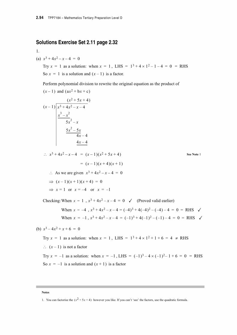
2.94 TPP7184 – Mathematics Tertiary Preparation Level D
Solutions Exercise Set 2.11 page 2.32
1.
(a)
Try as a solution: when , LHS = = RHS
So is a solution and is a factor.
Perform polynomial division to rewrite the original equation as the product of
and
= See Note 1
=
' As we are given
9
9 or x = –1
Checking:When , ✓ (Proved valid earlier)
When , ✓
When , ✓
(b)
Try as a solution: when , LHS = : RHS
' is not a factor
Try as a solution: when , LHS = = RHS
So is a solution and is a factor
Notes
1. You can factorise the however you like. If you can’t ‘see’ the factors, use the quadratic formula.
x3 4x2 x– 4–+ 0=
x 1= x 1= 13 4 12! 1– 4–+ 0=
x 1= x 1–% &
x 1–% & ax2 bx c+ +% &
x 1–% &
x2 5x 4+ +% &
x3 4x2 x– 4–+
x3
x2
–
5x2
x–-----------------
5x2
5x–
4x 4–--------------------
4x 4–---------------
' x3 4x2 x– 4–+ x 1–% & x2 5x 4+ +% &
x2 5x 4+ +% &
x 1–% & x 4+% & x 1+% &
x3 4x2 x– 4–+ 0=
x 1–% & x 1+% & x 4+% & 0=
x 1= or x 4–=
x 1= x3 4x2 x– 4–+ 0=
x 4–= x3 4x2 x– 4–+ 4–% &3= 4 4–% &2 4–% &– 4–+ 0 RHS= =
x 1–= x3 4x2 x– 4–+ 1–% &3 4 1–% &2 1–% &– 4–+ 0 RHS= = =
x3 4x2– x 6+ + 0=
x 1= x 1= 13 4 12! 1 6+ + + 4=
x 1–% &
x 1–= x 1–= 1–% &3 4 1–% &2! 1– 6+– 0=
x 1–= x 1+% &

Module 2 – Algebra & Geometry 2.95
Solutions Exercise Set 2.11 cont.
1. (b) continued
=
' As we are given
9
9
Checking: When has already been proved valid
When , ✓
When , ✓
(c)
Try as a solution: when , LHS = = RHS
So is a solution and is a factor
=
=
=
=
' As we are given
9
9
Checking:When has already been proved valid
When , ✓
When , ✓
x2 5– x 6+
x3 4– x2 x 6+ +
x3 x2+
5– x2 x+
5– x2 5x–
6x 6+-----------------------
------------------------
6x 6+---------------
(x + 1)
x3' 4x2– x 6+ + x 1+% & x2 5x– 6+% &=
x 1+% & x 3–% & x 2–% &
x3 4– x2 x 6+ + 0=
x 1+% & x 3–% & x 2–% & 0=
x 1–= , x 3 or x 2==
x 1–=
x 3= x3 4x2– x 6+ + 33 4 32! 3 6+ +– 0 RHS= = =
x 2= x3 4x2– x 6+ + 23 4 22! 2 6+ +– 0 RHS= = =
2x3 2x2– 8x– 8+ 0=
x 1= x 1= 2 13 2 12 8 1 8+!–!–! 0=
x 1= x 1–% &
2x2 8–
2x3 2x2– 8x– 8+
2x3 2x2–
8x– 8+
8x– 8+-------------------
-----------------------. .(x - 1)
2x3' 2x2– 8x– 8+ x 1–% & 2x2 8–% &
x 1–% & 2 x2 4–% &!
x 1–% & 2 x 2–% &! x 2+% &
x 1–% & 2x 4–% & x 2+% &
2x3 2– x2 8x– 8+ 0=
x 1–% & 2x 4–% & x 2+% & 0=
x 1= , x 2 or x 2–==
x 1=
x 2= 2x3 2x2– 8x– 8+ 2 23! 2 22! 8 2 8+!–– 0 RHS= = =
x 2–= 2x3 2x2– 8x– 8+ 2 2–% &3 2 2–% &2 8 2–% & 8+!–!–! 0 RHS= = =

2.96 TPP7184 – Mathematics Tertiary Preparation Level D
Solutions Exercise Set 2.11 cont.
(d)
Try as a solution: when , LHS = : RHS
' is not a factor
Try as a solution: when , LHS =
So is a solution and is a factor
=
=
' As we are given
9
9
Checking:When has already been proved valid
When , = 2 = RHS ✓See Note 1
When , ✓
Notes
1. Here I have checked by substituting in the original equation. This is a good idea in case an error has been made right back in the
beginning.
t3 3t2 6t– 6–+ 2=
t3 3t2 6t– 8–+' 0=
t 1= t 1= 13 3 12! 6 1 8–!–+ 14–=
t 1–% &
t 1–= t 1–= 1–% &3 3 1–% &2! 6 1–% &!– 8–+ 0 RHS= =
t 1–= t 1–% &
t2 2t 8–+
t3 3t2 6t– 8–+
t3 t2+
2t2 6t–------------------
2t2 2t+
8t– 8–------------------
8t– 8–------------------
(t + 1)
t3' 3t2 6t– 8–+ t 1+% & t2 2t 8–+% &
t 1+% & t 4+% & t 2–% &
t3 3t2 6t– 8–+ 0=
t 1+% & t 4+% & t 2–% & 0=
t 1–= , t 4–= or t 2=
t 1–=
t 4–= t3 3t2 6t– 6–+ 4–% &3 3 4–% &2 6 4–% &!– 6–!+=
t 2= t3 3t2 6t– 6–+ 23 3 22 6 2 6–!–!+ 2 RHS= = =

Module 2 – Algebra & Geometry 2.97
Solutions Exercise Set 2.11 cont.
(e)
Try as a solution: when , LHS = = RHS
So is a solution and is a factor
=
=
' As we are given
9
9
Checking:When has already been proved valid
When , LHS = and
RHS = = LHS ✓
When , LHS = and
RHS = = –2 = RHS ✓
y3 6+ 2y2= 5y+
y3 2y2– 5y– 6+' 0=
y 1= y 1= 13 2 12 5 1 6+!–!– 0=
y 1= y 1–% &
y2 y– 6–
y3 2y2– 5y– 6+
y3 y2–
y2– 5y–
y2– y+
6y– 6+-------------------
---------------------
6y– 6+-------------------
(y – 1)
y3 2y2 5y– 6+–' y 1–% & y2 y– 6–% &
y 1–% & y 3–% & y 2+% &
y3 2y2– 5y– 6+ 0=
y 1–% & y 3–% & y 2+% & 0=
y 1= , y 3= or y 2–=
y 1=
y 3= y3 6+ 33 6+ 33= =
2y2 5y+ 2 32!= 5 3!+ 33=
y 2–= y3 6+ 2–% &3 6+ 2–= =
2y2 5y+ 2 2–% &2 5 2–% &!+!=

2.98 TPP7184 – Mathematics Tertiary Preparation Level D
Solutions Exercise Set 2.11 cont.
2. (a)
(b)
P x% & x3 4x2 x– 4–+=
−5 −4 −3 −2 −1 0 1 2 3 4 5
−10
−6
−2
2
6
10
14
18
y
x
Roots arex = –4, –1 and 1
P x% & 2x3 2x2– 8x– 8+=
−5 −4 −3 −2 −1 0 1 2 3 4 5
−10
−6
−2
2
6
10
14
18
y
x
Roots arex = –2, 1 and 2

Module 2 – Algebra & Geometry 2.99
Solutions Exercise Set 2.11 cont.
(c)
(d)
P x% & 3x2 2x 1–+=
−5 −4 −3 −2 −1 0 1 2 3 4 5
−10
−6
−2
2
6
10
14
18
y
x
Roots arex = –1 and 1; 3
P x% & x3 2x2 x 2––+=
−5 −4 −3 −2 −1 0 1 2 3 4 5
−10
−6
−2
2
6
10
14
18
y
x
Roots arex = –2, –1 and 1

2.100 TPP7184 – Mathematics Tertiary Preparation Level D
Solutions Exercise Set 2.12 page 2.34
1.
Rational Fraction
Improper or proper
Not defined
(a) Yes Improper For x = 1
(b) No For x 0 and x = 1
(c) Yes Proper For x = 2 and x = 3
(d) Yes Proper For x = 0 and x = 1
(e) Yes Proper For x = –1, x = 0and x = 3
(f) Yes Improper For x = 2
(g) No
x2
x 1–-----------
x
x 1–-----------
x
x2 5x– 6+--------------------------
x
x 3+% & x 2–% &---------------------------------=
x2 1–
x x 1–% &2----------------------
7x 3+
x3 2x2– 3x–-------------------------------
7x 3+
x x 1+% & x 3–% &------------------------------------=
x3 3x 4–+
x 2–--------------------------
xcos
x2 x 1–+-----------------------

Module 2 – Algebra & Geometry 2.101
Solutions Exercise Set 2.13 page 2.36
1.
See Note 1
Checking: = = ✓
2.
Checking: = = ✓
3.
Checking:
= = ✓
Notes
1. The sums of proper rational functions are not unique. also equals .
x2 4x+
x2 2x+
2x-----------------
x2 4x+
x 2+-----------------' x
2x
x 2+------------+=
x2 4x+
x 2+----------------- x 2+% &=
x
x2 4x+
x 2+----------------- x 2
4
x 2+------------–+
x2x
x 2+------------+
x x 2+% & 2x+
x 2+--------------------------------
x2 2x 2x+ +
x 2+-----------------------------=
x2 4x+
x 2+-----------------
x3 2x– 1+
x2 4–--------------------------
x2 4–% & x3 2x– 1+
x3 4x–
2x 1+-----------------
=
x3 2x– 1+
x2 4–--------------------------' x
2x 1+
x2 4–---------------+=
x
x2x 1+
x2 4–---------------+
x x2 4–% & 2x 1+ +
x2 4–-------------------------------------------
x3 4x– 2x 1+ +
x2 4–--------------------------------------
x3 2x– 1+
x2 4–--------------------------=
x + 2
x3 3x–
x2 2x–----------------- =
x3 0x2 3x–+
x3 2x2–
2x2 3x–
2x2 4x–
x--------------------
--------------------
x3 3x–
x2 2x–-----------------' x 2
x
x2 2x–-----------------+ +=
(x2 – 2x)
x 2x
x2 2x–-----------------+ +
x x2 2x–% & 2 x2 2x–% & x++
x2 2x–-----------------------------------------------------------------=
x3 2x2 2x2 4x– x+ +–
x2 2x–-------------------------------------------------------
x3 3x–
x2 2x–-----------------
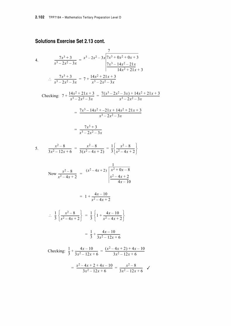
2.102 TPP7184 – Mathematics Tertiary Preparation Level D
Solutions Exercise Set 2.13 cont.
4.
Checking:
=
=
5. =
=
=
=
=
Checking:
= ✓
7x3 3+
x3 2x2– 3x–-------------------------------
7
x3 2x2– 3x– 7x3 0x2 0x 3+ + +
7x3 14x2 21x––
14x2 21x 3+ +-----------------------------------------
=
7x3 3+
x3 2x2– 3x–-------------------------------' 7
14x2 21x 3+ +
x3 2x2– 3x–------------------------------------+=
714x2 21x 3+ +
x3 2x2– 3x–------------------------------------+
7 x3 2x2– 3x–% & 14x2 21x 3+ + +
x3 2x2– 3x–----------------------------------------------------------------------------------=
7x3 14x2 21– x 14x2 21x 3+ + + +–
x3 2x2– 3x–---------------------------------------------------------------------------------------
7x3 3+
x3 2x2– 3x–-------------------------------
x2 8–
3x2 12x– 6+--------------------------------
x2 8–
3 x2 4x– 2+% &----------------------------------
1
3---
x2 8–
x2 4x– 2+--------------------------
3 45 67 8
=
Now x2 8–
x2 4x– 2+--------------------------
1
x2 0x 8–+
x2 4x– 2+
4x 10–--------------------------
x2 4x– 2+% &
14x 10–
x2 4x– 2+--------------------------+
1
3--- '
x2 8–
x2 4x– 2+--------------------------
3 45 67 8 1
3--- 1
4x 10–
x2 4x– 2+--------------------------+
3 45 67 8
1
3---
4x 10–
3x2 12x– 6+--------------------------------+
1
3---
4x 10–
3x2 12x– 6+--------------------------------+
x2 4x– 2+% & 4x 10–+
3x2 12x– 6+-------------------------------------------------------=
x2 4x– 2 4x 10–+ +
3x2 12x– 6+---------------------------------------------------
x2 8–
3x2 12x– 6+--------------------------------=

Module 2 – Algebra & Geometry 2.103
Solutions Exercise Set 2.14 page 2.46
1.
Step 1: {Product of two non-identical linear factors}
Step 2:
Step 3:
Step 5: From , A = 2B – 3 substituting in ! gives 2(2B – 3) – B = –1
' 4B – 6 – B = –1 ' 3B = 5 ' B =
Step 6:
Step 7: Checking:
Step 4: ' –A + 2B = 3 _______
and 2A – B = –1 ______!
3 x–
2 x– ! 2x 1– !------------------------------------
P x !Q x !------------=
Q x ! 2 x– ! 2x 1– !=
3 x–
2 x– ! 2x 1– !------------------------------------
A
2 x– !----------------
B
2x 1– !-------------------+=
3 x–
2 x– ! 2x 1– !------------------------------------
A 2x 1– ! B 2 x– !+
2 x– ! 2x 1– !---------------------------------------------------=
2Ax A– 2B Bx–+
2 x– ! 2x 1– !-----------------------------------------------=
2A B– !x A– 2B+ !+
2 x– ! 2x 1– !-----------------------------------------------------------=
Equating coefficients of power of x" #$ %& '
5
3--- A( 2
5
3--- 3
1
3---=–)=
3 x+
2 x– ! 2x 1– !------------------------------------*
A
2 x– !----------------
B
2x 1– !-------------------+=
1 3+2 x–-----------
5 3+2x 1–---------------+=
1
6 3x–---------------
5
6x 3–---------------+=
1
6 3x–---------------
5
6x 3–---------------+
1 6x 3– !) 5 6 3x– !)+
6 3x– ! 6x 3– !----------------------------------------------------------------=
6x 3– 30 15x–+
3 2 x– ! 3 2x 1– !)-------------------------------------------------=
9x– 27+
9 2 x– ! 2x 1– !----------------------------------------=
x– 3+
2 x– ! 2x 1– !------------------------------------= ✓

2.104 TPP7184 – Mathematics Tertiary Preparation Level D
Solutions Exercise Set 2.14 cont.
2.
Step 1: {Product of three non-identical linear factors}
Step 2:
Step 3:
Step 4: Equating coefficients of powers of x
* A + B + C = 0
–3A – 6B + 3C = 9
–18A = –72
Step 5: Solving (not shown here) yields A = 4 ; B = ; C =
Step 6:
9x 72–
x3 3x2– 18x–----------------------------------
P x !Q x !------------=
Q x ! x3 3x2– 18x–=
x x2 3x– 18– !=
x x 3+ ! x 6– !=
9x 72–
x3 3x2– 18x–----------------------------------
A
x !-------
B
x 3+ !----------------
C
x 6– !----------------+ +=
9x 72–
x3 3x2– 18x–----------------------------------
A x 3+ ! x 6– ! Bx x 6– ! Cx x 3+ !+ +
x ! x 3+ ! x 6– !---------------------------------------------------------------------------------------------------=
A x2 3x– 18– ! Bx2 6Bx– Cx2 3Cx+ + +
x ! x 3+ ! x 6– !-------------------------------------------------------------------------------------------------------=
Ax2 3Ax 18A Bx2 6Bx Cx2 3Cx+ +–+––
x ! x 3+ ! x 6– !------------------------------------------------------------------------------------------------------------=
A B C+ + !x2 3A 6B 3C+–– !x 18A– !++
x ! x 3+ ! x 6– !----------------------------------------------------------------------------------------------------------------=
11–
3---------
1–
3------
9x 72–
x3 3x2 18x––----------------------------------
4
x---
11– 3+x 3+
----------------1– 3+
x 6–-------------+ +
4
x---
11
3 x 3+ !--------------------
1
3 x 6– !-------------------––= =

Module 2 – Algebra & Geometry 2.105
Solutions Exercise Set 2.14 cont.
2. continued
Step 7: Checking:
3.
Step 1: {Product of one linear factor and one quadratic factor}
Step 2:
Step 3:
Step 4: Equating coefficients of powers of x
A – B = 1
2B – C = –3
A + 2C = 12
4
x---
11
3 x 3+ !--------------------–
1
3 x 6– !-------------------–
4 3 ! x 3+ ! 3 ! x 6– ! 11 x ! 3 ! x 6– ! 1 x !– 3 ! x 3+ !–
x.3. x 3+ !.3. x 6– !----------------------------------------------------------------------------------------------------------------------------------------=
(I have not found the L.C.D. here)
36 x 3+ ! x 6– ! 33x x 6– !– 3x x 3+ !–
9x x 3+ ! x 6– !-----------------------------------------------------------------------------------------------------=
36 x2 3x– 18– ! 33x2 198x+– 3x2 9x––
9x x 3+ ! x 6– !------------------------------------------------------------------------------------------------------=
36x2 108x– 648– 33x2 198x 3x2 9x––+–
9x x 3+ ! x 6– !-----------------------------------------------------------------------------------------------------------=
81x 648–
9x x 3+ ! x 6– !----------------------------------------=
9 9x 72– !9x x 3+ ! x 6– !----------------------------------------=
9x 72–
x x 3+ ! x 6– !------------------------------------= ✓
x2 3x 12+–
2 x– ! 1 x2+ !------------------------------------
P x !Q x !------------=
Q x ! 2 x– ! 1 x2+ !=
x 3x– 12+
2 x– ! 1 x2+ !------------------------------------
A
2 x– !----------------
Bx C+
1 x2+ !-------------------+,
x2 3x– 12+
2 x– ! 1 x2+ !------------------------------------
A 1 x2+ ! Bx C+ ! 2 x– !+
2 x– ! 1 x2+ !---------------------------------------------------------------------=
A Ax2 2Bx Bx2– 2C Cx–+ + +
2 x– ! 1 x2+ !-------------------------------------------------------------------------------=
A B– !x2 2B C– !x A 2C+ !+ +
2 x– ! 1 x2+ !-------------------------------------------------------------------------------------=
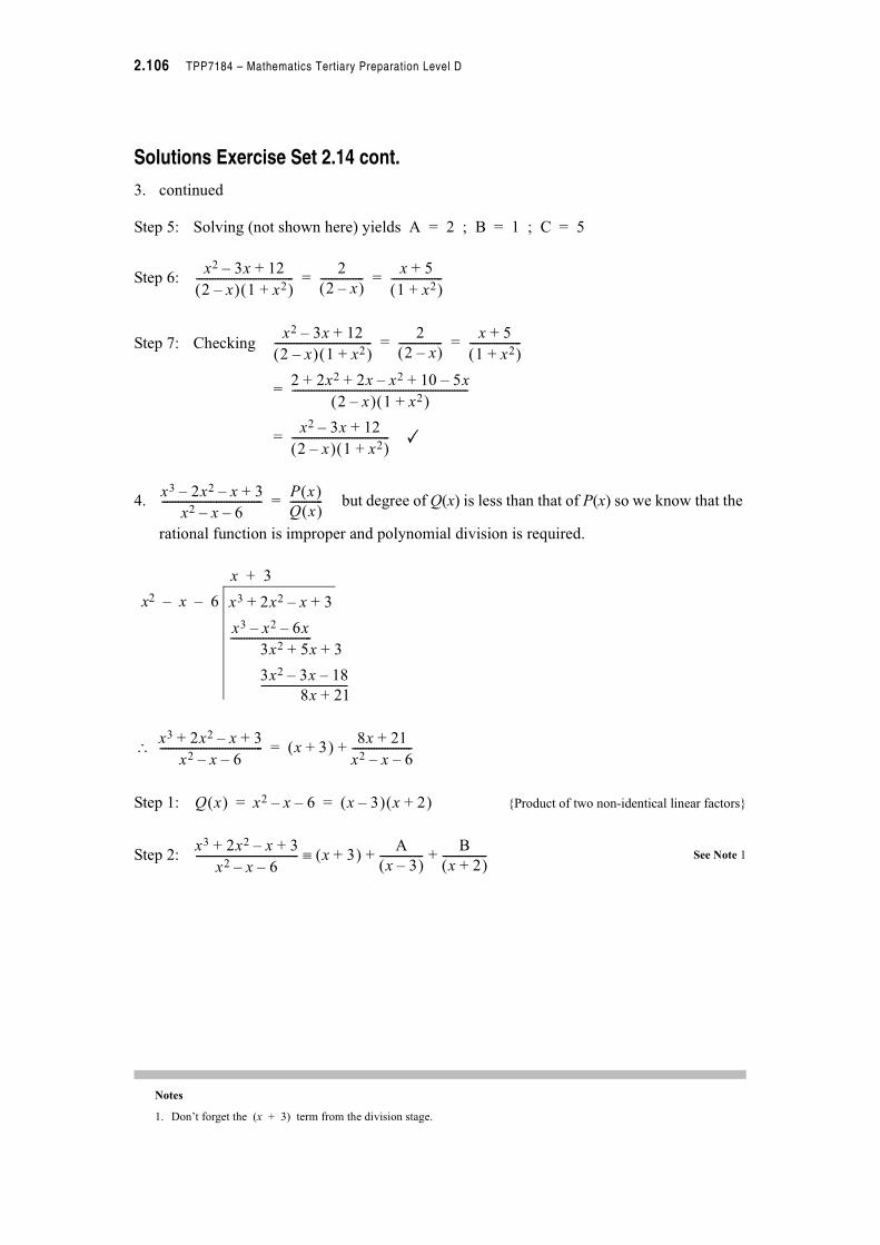
2.106 TPP7184 – Mathematics Tertiary Preparation Level D
Solutions Exercise Set 2.14 cont.
3. continued
Step 5: Solving (not shown here) yields A = 2 ; B = 1 ; C = 5
Step 6:
Step 7: Checking
4. but degree of Q(x) is less than that of P(x) so we know that the
rational function is improper and polynomial division is required.
Step 1: {Product of two non-identical linear factors}
Step 2: See Note 1
Notes
1. Don’t forget the (x + 3) term from the division stage.
x2 3x– 12+
2 x– ! 1 x2+ !------------------------------------
2
2 x– !----------------
x 5+
1 x2+ !-------------------= =
x2 3x– 12+
2 x– ! 1 x2+ !------------------------------------
2
2 x– !----------------
x 5+
1 x2+ !-------------------= =
2 2x2 2x x2 10 5x–+–+ +
2 x– ! 1 x2+ !-----------------------------------------------------------------=
x2 3x– 12+
2 x– ! 1 x2+ !------------------------------------= ✓
x3 2x2 x 3+––
x2 x– 6–-------------------------------------
P x !Q x !------------=
x3 2x2 x 3+–+
x3 x2– 6x–
3x2 5x 3+ +------------------------------
3x2 3x– 18–
8x 21+--------------------------------
x + 3
x2 – x – 6
x3 2x2 x 3+–+
x2 x– 6–--------------------------------------* x 3+ !
8x 21+
x2 x– 6–----------------------+=
Q x ! x2 x– 6– x 3– ! x 2+ != =
x3 2x2 x 3+–+
x2 x– 6–-------------------------------------- x 3+ !
A
x 3– !----------------
B
x 2+ !----------------+ +,

Module 2 – Algebra & Geometry 2.107
Solutions Exercise Set 2.14 cont.
4. continued
Step 3:
Step 4: Equating coefficients of powers of x from Step 3. See Note 1
A + B = 8
2A – 3B = 21
Step 5: Solving (not shown here) yields A = 9 ; B = –1
Step 6: See Note 2
Step 7: Checking
Notes
1. Remember that you are equating coefficients of powers of x from the remainder.
2. Remember the (x + 3) term.
8x 21+
x2 x– 6–----------------------
A x 2+ ! B x 3– !+
x 3– ! x 2+ !------------------------------------------------=
Ax 2A Bx 3B–+ +
x 3– ! x 2+ !------------------------------------------------=
A B+ !x 2A 3B– !+
x 3– ! x 2+ !------------------------------------------------------=
8x 21+
x2 x– 6–----------------------
9
x 3– !----------------
1–
x 2+ !----------------+=
x3 2x2 x 3+–+
x2 x– 6–--------------------------------------* x 3+ !
9
x 3– !----------------
1
x 2+ !----------------–+=
x 3+ !9
x 3– !----------------
1
x 2+ !----------------–+
x 3+ ! x 3– ! x 2+ ! 9 x 2+ !) 1 x 3– !)–+
x 3– ! x 2+ !-------------------------------------------------------------------------------------------------------------------=
x2 9– ! x 2+ ! 9x 18 x 3+–+ +
x 3– ! x 2+ !-------------------------------------------------------------------------------=
x3 2x2 9x 18 9x 18 x 3+–+ +––+
x 3– ! x 2+ !--------------------------------------------------------------------------------------=
x3 2x2 x 3+–+
x 3– ! x 2+ !--------------------------------------= ✓

2.108 TPP7184 – Mathematics Tertiary Preparation Level D
Solutions Exercise Set 2.14 cont.
5.
Step 1:
{Product of two identical linear factors and one other linear factor}
Step 2:
Step 3: See Note 1
Step 4: Equating coefficients of powers of x
4A – 2B = 0
–4A – B + C = 9
A + B + C = 0
Step 5: Solving (not shown here) yields A = –1 ; B = –2 ; C = 3
Step 6:
Step 7: Checking
Notes
1. Take care finding the lowest common denominator.
9x
1 x+ ! 1 2x– !2---------------------------------------
P x !Q x !------------=
Q x ! 1 x+ ! 1 2x– !2 1 x+ ! 1 2x– ! 1 2x– != =
9x
1 x+ ! 1 2x– !2---------------------------------------
A
1 x+ !----------------
B
1 2x– !-------------------
C
1 2x– !2----------------------+ +,
9x
1 x+ ! 1 2x– !2---------------------------------------
A 1 2x– !2 B 1 x+ ! 1 2x– ! C 1 x+ !+ +
1 x+ ! 1 2x– !2------------------------------------------------------------------------------------------------------=
A 1 4x 4x2+– ! B 1 2x x 2x2–+– ! C Cx+ + +
1 x+ ! 1 2x– !2---------------------------------------------------------------------------------------------------------------------=
A 4Ax 4Ax2 B Bx2 Bx2– C Cx+ +–+ +–
1 x+ ! 1 2x– !2----------------------------------------------------------------------------------------------------------=
4A 2B– !x2 4A– B C+– !x A B C+ + !+ +
1 x+ ! 1 2x– !2------------------------------------------------------------------------------------------------------------------=
9x
1 x+ ! 1 2x– !2---------------------------------------
1–
1 x+ !----------------
2–
1 2x– !-------------------
3
1 2x– !2----------------------+ +=
1–
1 x+ !----------------
2–
1 2x– !-------------------
3
1 2x– !2----------------------+ +
1– 1 2x– !2 2 1 x+ ! 1 2x– !) 3 1 x+ !)+–)1 x+ ! 1 2x– !2
-----------------------------------------------------------------------------------------------------------------------=
1– 4x 4x– 2 2 2x+ ! 1 2x– ! 3 3x+ +–+
1 x+ ! 1 2x– !2------------------------------------------------------------------------------------------------------=
1– 4x 4x– 2 2 4x 2x 4x2 3 3x+ + +–+–+
1 x+ ! 1 2x– !2--------------------------------------------------------------------------------------------------------=
9x
1 x+ ! 1 2x– !2---------------------------------------= ✓

Module 2 – Algebra & Geometry 2.109
Solutions Exercise Set 2.14 cont.
6. (a)
Step 1: {Product of two non-identical linear factors}
Step 2:
Step 3:
Step 4:
Step 5: Solving (not shown here) yields A = 1 ; B = –1
Step 6:
(b)
=
=
=
=
As
1
r r 1+ !-------------------
P r !Q r !-----------=
Q r ! r r 1+ !=
1
r r 1+ !-------------------
A
r----
B
r 1+-----------+,
1
r r 1+ !-------------------
A r 1+ ! Br+
r r 1+ !)----------------------------------,
Ar A Br+ +
r r 1+ !------------------------------=
r A B+ ! A+
r r 1+ !---------------------------------=
A B+ 0=
A 1=
1
r r 1+ !-------------------
1
r---
1
r 1+-----------–=
1
r r 1+ !-------------------
1
r---
1
r 1+-----------–=
Sn*1
r r 1+ !-------------------
r 1=
n
-=1
r---
1
r 1+-----------–
r 1=
n
-
1
r---
1
r 1+-----------
r 1=
n
-–
r 1=
n
-
1
1---
1
2---
1
3---
1
4--- .
1
n---+ + + + +
/ 01 23 4 1
2---
1
3---
1
4--- .
1
n---
1
n 1+------------+ + + + +
/ 01 23 4
–
Sn* 11
n 1+------------–
n 5, 1
n 1+------------ 0 Sn 16* 0–6 6
S5* 1=

2.110 TPP7184 – Mathematics Tertiary Preparation Level D
Solutions Exercise Set 2.15 page 2.60
Examine the graphs for each of these problems and make sure that the algebra and geometry ‘match’.1. y = 2x + 4 __________
y = 8x – 2 _________!
* 2x + 4 = 8x – 2
* –6x = –6
* x = 1
When x = 1, Equation gives y = 2 ) 1 + 4 = 6* x = 1, y = 6 is the solution
Checking: Equation RHS = 2 ) 1 + 4 = 6 = LHS ✓
Equation ! RHS = 8 ) 1 – 2 = 6 = LHS ✓
2. y = 2x – 4
y = 2x + 6
These lines have the same slope * they will not have a point of intersection (7no solution which satisfies both equations.
y
x
x
y

Module 2 – Algebra & Geometry 2.111
Solutions Exercise Set 2.15 cont.
3. (x – 2)2 + (y – 4)2 = 16__________
x = 3 ___________ !
Substituting in Equation for x gives
Checking: Equation when x = 3 and
LHS = (3 – 2)2 + = 12 + = 16 = RHS ✓
Equation ! when x = 3 and
LHS = (3 – 2)2 + = 12 + = 16 = RHS ✓
3 2– !2 y 4– !2+ 16=
1 y 4– !2 16=+*
y 4– !2 15=*
y 4– 158=*
y* 15 4 or y+ 15– 4+= =
x* 3, y 15 4 and x 3, y 15– 4 are the solutions+==+= =
y 15– 4+=
15 4 4–+ !2 15 !2
y 15– 4+=
15– 4 4–+ !215– !2
y
x

2.112 TPP7184 – Mathematics Tertiary Preparation Level D
Solutions Exercise Set 2.15 cont.
4. x2 + y2 = 1__________
(x – 3)2 + y2 = 4__________ !
Subtracting equation from equation ! gives
(x – 3)2 – x2 = 3
* x2 – 6x + 9 – x2 = 3
* –6x = –6
* x = 1
Substituting in Equation for x gives
12 + y2 = 1
y2 = 0
y = 0
There is only one solution, x = 1, y = 0
Checking: Equation , LHS = 12 9 02 = 1 = RHS ✓
Equation !, LHS = (1 – 3)2 + 02 = (–2)2 = 4 = RHS ✓
x
y
x2 + y2 = 1 (x – 3)2 + y2 = 4

Module 2 – Algebra & Geometry 2.113
Solutions Exercise Set 2.15 cont.
5. x2 + y2 – 4x + 2y + 4 = 0 __________ See Note 1
y = –3x ________!
Substituting for y in Equation using y = –3x from Equation !
x2 + (–3x)2 – 4x + 2(–3x) + 4 = 0
x2 + 9x2 – 4x – 6x + 4 = 0
* 10x2 – 10x + 4 = 0
* 5x2 – 5x + 2 = 0
*
This is impossible so there is no solution which satisfies both equations. The graph below shows that the line does not intersect with the circle.
Notes
1. It would be difficult to visualise the graph of this equation if you had not used the Hint given in the question. By
completing the square it becomes obvious that the circle is centred at (2, –1) and has radius of 1. Getting an equation
into a standard form that you can recognise is a very powerful tool.
x5– !– 5– !2 4 5 2))–8
2 5)-------------------------------------------------------------------=
2 15–810
----------------------=
y
x
x2 + y2 – 4x + 2y + 4 = 0
y = –3x

2.114 TPP7184 – Mathematics Tertiary Preparation Level D
Solutions Exercise Set 2.15 cont.
6. General form of a circle is
(x – h)2 + (y – k)2 = r2
As (0, 0) is on the circle
(0 – h)2 + (0 – k)2 = r2
i.e. h2 + k2 = r2
As (0, 3) is on the circle
(0 – h)2 + (3 – k)2 = r2
i.e. h2 + 9 – 6k + k2 = r2
As (1, 0) is on the circle
(1 – h)2 + (0 – k)2 = r2
i.e. 1 – 2h + h2 + k2 = r2
Now we have three equations in h, k and r to solve simultaneously
h2 + k2 = r2____________________________
h2 + 9 – 6k + k2 = r2 ________________!
h2 + 1 – 2h + k2 = r2________________"
From , k2 = r2 – h2 _____________________#
Substituting in " for k2 gives
h2 + 1 – 2h + r2 – h2 = r2
* 1 – 2h = 0
* h = ½
Substituting in ! for h gives
(½)2 + 9 – 6k + k2 = r2 _____________$
From #, k2 = r2 – (½)2
* k2 = r2 – (¼)
Substituting in $ for k2 gives
¼ + 9 – 6k + r2 – ¼ = r2
* 9 – 6k = 0
* k =
Substituting in for h and k gives
(½)2 + = r2
* r2 = ¼ + = =
* The circle has the equation
(x – ½)2 + (y – )2 =
32+
( 32+ )2
94+ 10
4+ 52+
32+ 5
2+
y
x

Module 2 – Algebra & Geometry 2.115
Solutions Exercise Set 2.15 cont.
6. continued
Solving (x – ½)2 + (y – )2 = and
y = ln x
looks complicated and indeed cannot be done algebraically. So the graphical method will be used. You could also do it numerically using guess and check.)
Zooming in on the points of intersection gives x = 1, y = 0 and x 1.8, y 0.6as the solutions.
Remember to check the solutions by substituting in each of the original equations.‘
32+ 5
2+
(1, 0)
(1.8, 0.6)
y
x
x1
2---–/ 0
3 42
y3
2---–/ 0
3 42
+5
2---=
: :

2.116 TPP7184 – Mathematics Tertiary Preparation Level D
Solutions Exercise Set 2.15 cont.
7. y = e–x_____________
y = _______ !
Using the Hint rewrite Equation ! as y = _______ "
which is the equation to a hyperbola. This hyperbola is shown below.
The graphical technique looks appropriate for solving the equations. Note that the hyperbola is restricted to the LH branch because it is defined for x < 1 only.
Zooming in on the point of intersection gives the solution x –1.2, y 3.3
Check this solution.
3
1 x–----------- 2+
3–
x 1–----------- 2+
x
y
x
y
: :

Module 2 – Algebra & Geometry 2.117
Solutions Exercise Set 2.15 cont.
8. y = ___________
y = _____________ !
Rewrite Equation to give the equations for each branch of the graph of y = .
• The LH branch has equationy1 = –2x for x ; 0• The RH branch has equationy2 = 2x for x < 0
Then solve Case (i) y1 = –2x and for x ; 0
and Case (ii) y2 = 2x and for x < 0
Case (i)
y1 = –2x for x ; 0
* –2x = * x2 = –1
This is impossible so there is no point of intersection of the hyperbola with the LH branch of y =
Case (ii)
y2 = 2x for x < 0
* 2x = * x2 = 1 * x = +1 or x = –1
But y2 = 2x is defined for x < 0, therefore there is only one solution and this occurs whenx = 1 and y = 2.
Check this result with the graphs of y = and
2x
2
x---
2x
y2
x---=
y2
x---=
y2
x---=
2
x---
2x
y2
x---=
2
x---
2x y2
x---=
y
x
y = 2x
y =2
x---

2.118 TPP7184 – Mathematics Tertiary Preparation Level D
Solutions Exercise Set 2.15 cont.
9. Rewriting (x + 1)(2 – x) = 5 ln (1 + x) as two functions
y1 = (x + 1)(2 – x) and
y2 = 5 ln (1 + x)
when y1 = y2 the solution to the original equation is found.
y1 = (x + 1)(2 – x) is a parabola cutting the x-axis at x – 1 and x = 2 with a maximum
turning point and axis of symmetry at x = .
y2 = 5 ln (1 + x) is a logarithmic curve.
The graphical solution method will be easiest.
One solution only for y1 and y2 at x = 0.6 and y = 2.35 * approximate solution to original equation is x = 0.6.
Checking: LHS of original equation = (x + 1)(2 – x) = (0.6 + 1) (2 – 0.6) = 2.24RHS of original equation = 5 ln (1 + x) = 5 ln (1 + 0.6) = 2.35
You can improve the accuracy of the solution by zooming in further on the intersection point of y1 and y2
1
2---
(0.6, 2.35)
x
y

Module 2 – Algebra & Geometry 2.119
Solutions Exercise Set 2.16 page 2.64
1. Graph Function One-to-one Graph Function One-to-one
(a)
(b)
(c)
(d)
(e)
(f)
(g)
(h)
(i)
(j)
(k)
Yes
Yes
Yes
Yes
Yes
Yes
Yes
Yes
Yes
Yes
Yes
Yes
Yes
Yes
No
Yes
No
Yes
No
Yes
Yes
Yes
(l)
(m)
(n)
(o)
(p)
(q)
(r)
(s)
(t)
(u)
(v)
Yes
Yes
Yes
Yes
Yes
Yes
Yes
Yes
No
Yes
Yes
Yes
Yes
Yes
Yes
Yes
No
Yes
Yes
Yes
No
Graph Inverse
(a)
(g)
(m)
(n)
(b)
(i)
(p)
(u)

2.120 TPP7184 – Mathematics Tertiary Preparation Level D
Solutions Exercise Set 2.16 cont.
2. (i)
(ii) Choose, say, x = 8, Step (1): f–1(8) = 2 (reading from graph)
Step (2): f(f–1(8)) = f(2) = 8 (reading from graph)
Choose, say, x = 14, Step (1): f–1(14) = 4 (reading from graph)
Step (2): f(f–1(14)) = f(4) = 14 (reading from graph)
For the two values chosen for x (and, in fact for any value of x)
f(f–1(x)) = x
(iii) Following the same procedure but doing Step 2 first and then Step 1 shows that
f(f–1(x)) = x
f(x) = 3x + 2
y
x
(2)
(2)
f–1(x) = 1/3(x – 2)
(1)
(1)

Module 2 – Algebra & Geometry 2.121
Solutions Exercise Set 2.17 page 2.68
1. If f(x) is the height of a person who weighs x kg,
f–1(x) is the weight of a person whose height is x cm See Note 1
So f–1(100) is the weight of a person who is 100 cm tall.
2. (i) f(d) will not have an inverse as many different odometer readings will have the same
number of litres in the tank depending on when it was last filled (i.e. f(d) is not a
one-to-one function).
(ii) The same number of people may be in the stores at say 12.10, 12.30, 12.50 etc. so
f(t) is not a one-to-one function and hence does not have an inverse.
(iii) There is a direct and unique relationship between the number of kilograms of ice and
the volume it occupies. So f(x) is a one-to-one function and its inverse exists.
(iv) Several first year students can have birthdays on the same day of the year. So f(n) is
not a one-to-one function and hence does not have an inverse.
(v) The heavier the letter the more it costs to post so f(w) is a one-to-one function and
its inverse exists. [An assumption has been made here about the pricing policy for the
mailing.]
If you had trouble with any of these questions try to work backwards e.g. in (iv). (f you were given a birthday could you uniquely identify the student? Obviously not! But in (iii) if you know the volume of ice you can determine exactly the mass of ice.3. (i) There is a unique value of f(x) for each x value i.e. there is a one-to-one mapping
from x to f(x) so f(x) will have an inverse.
(ii) Domain of f(x) is the Set D = {1, 2, 3, 4, 5, 6, 7} and the range of f(x) is the
Set R = {3, –7, 19, 4, 178, 2, 1}
The domain of f–1(x) will be the same as the range of f(x)
i.e. {3, –7, 19, 4, 178, 2, 1} and the range of f(x) is {1, 2, 3, 4, 5, 6, 7}
Notes
1. Technically f(x) is the mass of the person. (Weight is a force)
1
2
3
4
5
6
7/ 01 21 21 21 21 21 21 21 21 21 23 4 3
7–
19
4
178
2
1/ 01 21 21 21 21 21 21 21 21 21 23 4
x f(x)
f

2.122 TPP7184 – Mathematics Tertiary Preparation Level D
Solutions Exercise Set 2.17 cont.
4. f(x) = x2 + 3x
(i) This is the equation of a parabola so there will be two values of x that give the same
value of f(x). [Recall that a parabola is symmetric about its axis of symmetry which
in this case is at e.g. and both give
(ii) Any domain which does not include the turning point will allow the inverse to be
found. As the turning point will be on the axis of symmetry, this implies that any part
of the domain or any part of the domain will be satisfactory.
(iii) Choose say
x3–
2------= x
1–
2------= x
5–
2------= f x !
5–
4------=
x3–
2------< x
3–
2------;
3–
2------ x 2; ;
f(x) = x2 + 3x
x
y
f–1(x)3–
2------ 0=/ 0
3 4

Module 2 – Algebra & Geometry 2.123
Solutions Exercise Set 2.17 cont.
5. C(P) = 100 + 2P
(i) The domain should be restricted because making a negative number of articles is
nonsense. So P <70 is the domain. It also seems that there would be restrictions on
the amount of inventory that can be held, the number of items the current machinery
and labour can produce etc. thus there would be an upper limit also on P.
(ii) C = 100 + 2P
Reversing variables gives
P = 100 + 2C [Note: You are not rearranging the original equation]
* Solving for C gives
(iii) The number of articles that can be produced for a given amount of money.
6. (i) f(x) = 2 + 3x
i.e. y = 2 + 3x
Reversing variables: x = 2 + 3y
* x – 2 = 3y
* y =
i.e.
Checking f(f–1(x)) = f
= 2 + 3
= 2 + x – 2
= x ✓
(ii) f(x) = 1 – x2 for x <70i.e. y = 1 – x2
Checking f–1(f(x)) = f–1(1 – x2)
=
=
= x ✓
CP 100–
2------------------=
C 1– P !*1
2---P 50–=
x
3---
2
3---–
f 1– x !x
3---
2
3---–=
x
3---
2
3---–/ 0
3 4
x
3---
2
3---–/ 0
3 4
Reversing variables: x = 1 – y2
* y2 = 1 – x
* y =
i.e. f–1(x) =
1 x–
1 x–
{only concerned with positive root because of restriction on domain of f(x)}
1 1 x2– !–
1 1 x2+–

2.124 TPP7184 – Mathematics Tertiary Preparation Level D
Solutions Exercise Set 2.17 cont.
(iii) f(x) = 50e0.1x
i.e. y = 50e0.1x
Reversing variables: x = 50e0.1y
* ln = 0.1y
* y = 10 ln
i.e.
Checking f(f–1(x)) = f(10 ln )
= 50e0.1 ) 10 ln (x/50)
= 50eln (x/50)
= 50 )7
= x ✓
(iv) f(x) = 2x3 – 4 [Note: Need to be careful that the
i.e. y = 2x3 – 4 inverse exists – a rough sketch helps]
x
50------/ 0
3 4
x
50------
f 1– x ! 10lnx
50------/ 0
3 4=
x
50------
x
50------
Reversing variables: x = 2y3 – 4
* x + 4 = 2y3
* y =
i.e. f–1(x) =
Checking f–1(f(x)) = f–1(2x3 – 4)
=
=
= (x3)1/3
= x ✓
x 4+
2------------/ 0
3 41 3+
x 4+
2------------/ 0
3 41 3+
2x3 4 4+–
2--------------------------/ 0
3 41 3+
2x3
2--------/ 0
3 41 3+
y
x

Module 2 – Algebra & Geometry 2.125
Solutions Exercise Set 2.17 cont.
(v) f(x) = for x <70i.e. y =
Reversing variables: x =
* log2x = log2
= y2 – 1
* 1 + log2x = y2
* y =
Checking f(f–1(x)) =
=
=
=
= x ✓
2x2 1–
2x2 1–
2y2 1–
2y2 1–
1 log2x+
f 1 log2x+ !
21 log2x+/ 0
3 42
1–
21 log2x 1–+
2log2x
x
y
(only concerned with positive root)

2.126 TPP7184 – Mathematics Tertiary Preparation Level D
Solutions Exercise Set 2.18 page 2.73
1. (i)
* As exists and equals –1
(ii)
* As exists and equals 1
Note: This becomes obvious if is simplified before the limit as is found.
approaching x = –1from the negative side
approaching x = –1from the positive side
x –1.1 –1.01 –1.001 –0.999 –0.99 –0.9
f(x) = x3 – 2 –0.79 –0.9799 –0.997999 –1.001999 –1.0199 –1.19
approaching x = 0from the negative side
approaching x = 0from the positive side
x –0.2 –0.1 –0.001 0.01 0.1 0.2
f(x) = 0.8 0.9 0.999 1.01 1.1 1.2
limx 1––6
x2 2– ! 1–= ; limx 1+–6
x2 2– ! 1–=
limx 1––6
f x ! limx 1+–6
f x ! 1– limx 1–6
f x !(= =
x2 x+
x--------------
limx 0–6
x2 x+
x--------------/ 0
3 4 1= ; limx 0+6
x2 x+
x--------------/ 0
3 4 1=
limx 0–6
f x ! limx 0+6
f x ! 1 limx 06
f x !(= =
x2 x+
x-------------- x 06
x2 x+
x--------------
x2
x-----
x
x--+ x 1+= =
* limx 06
x 1+ 1=

Module 2 – Algebra & Geometry 2.127
Solutions Exercise Set 2.18 cont.
(iii)
* As exists and equals –6
Note: This becomes obvious if is simplified before the limit as is found.
(iv) See Note 1
* As exists and equals 1
This is an interesting and important example where the function is not defined at
x = 0 but the limit does exist at x = 0.
approaching x = –3from the positive side
approaching x = –3from the negative side
x –2.5 –2.9 –2.99 –3.01 –3.1 –3.5
f(x) = –5.5 –5.9 –5.99 –6.01 –6.1 –6.5
Notes
1. Because f(x) is a mixture of a trigonometric function and an algebraic function x must be in radians.
approaching x = 0from the negative side
approaching x = 0from the positive side
xSee Note 1
–0.2 –0.1 –0.01 0.01 0.1 0.2
f(x) = 1.0135502 1.0033467 1.0000333 1.0000333 1.0033467 1.0135502
x2 9–
x 3+--------------
limx 3– +
x2 9–
x 3+-------------- 6–= ; lim
x 3– –
x2 9–
x 3+-------------- 6–=
limx 3– +
f x! " limx 3– –
f x! " 6– limx 3–
f x! "#= =
x2 9–
x 3+-------------- x 3–
x2 9–
x 3+--------------
x 3–! " x 3+! "x 3+! "
--------------------------------- x 3–= =
$ limx 3–
x 3– 6–=
xtan
x------------
limx 0–
xtan
x------------% &' ( 1= ; lim
x 0+
xtan
x------------% &' ( 1=
limx 0–
f x! " limx 0+
f x! " 1 limx 0
f x! "#= =

2.128 TPP7184 – Mathematics Tertiary Preparation Level D
Solutions Exercise Set 2.18 cont.
2. (i) • exists as
• But f(x) is not continuous at because
(ii) • does not exist as
• Because the does not exist, f(x) is not continuous at
(iii) • exists as
• Because the exists and equals f(c), f(x) is continuous at
(iv) • does not exist as
• Because the does not exist, f(x) is not continuous at x = c
Note: This is the graph of the ‘greatest integer less than x’ function. The sumbol
used is [x].
So for y = [x] some coordinates are (3.2, 3), (3.7, 3), (–2.45, –3), (–4, –5)
3. (i)
and
$ As does not exist # f(x) is not continuous at x = 0
(ii)
and
$ As exists and equals 2
Now f(1) = 2 $ As is continuous as x = 1
limx c
f x! " limx c+
f x! " limx c–
f x! "=
x c= f c! " limx c
f x! ")
limx c
f x! " limx c+
f x! " limx c–
f x! ")
limx c
f x! " x c=
limx c
f x! " limx c+
f x! " limx c–
f x! "=
limx c
f x! " x c=
limx c
f x! " limx c+
f x! " limx c–
f x! ")
limx c
f x! "
f x! "2x 1+
2x*+,
=if x 0-
if x 0.c 0=
limx 0+
f x! " limx 0+
2x 0== limx 0–
f x! " limx 0–
2x 1+! " 1= limx 0
f x! ")=
limx 0
f x! "
f x! "
3x 1–
2
2x*/+/,
=
if x 10
if x = 1
if x 1.
c 1=
limx 1+
f x! " limx 1+
2x 2== limx 1–
f x! " limx 1–
3x 1–! " 2==
limx 1+
f x! " limx 1–
f x! " 2 limx 1
f x! "#==
limx 1
f x! " f 1! " 2 f x! "#==

Module 2 – Algebra & Geometry 2.129
Solutions Exercise Set 2.18 cont.
3. continued
(iii)
and
$ As exists and equals 5
Now f(–1) = 2 $ As is not continuous as x = –1
If you have trouble with any of these solutions draw the graphs so you can see clearly what is happening at x = c . You can also use the graphs to validate your answers.4.
The particular values of x where ‘something interesting’ is happening is where the different functions come together to define f(x) i.e. at x = 2 and x = 4.
Consider x = 2
and exists.
Now f(2) = 2x + 1 when x = 2 i.e. f(2) = 2 1 2 + 1 = 5
So f(x) is continuous at x = 2
Consider x = 4
and does not
exist $ f(x) is not continuous at x = 4
f x! "
x2 4+
2
3x– 2+*/+/,
=
if x 1–0
if x = 1–
if x 1–.
c 1–=
limx 1– +
f x! " limx 1– +
3– x 2+ 5== limx 1– –
f x! " limx 1– –
x2 4+ 5==
limx 1– +
f x! " limx 1– –
f x! " 5 limx 1–
f x! "#==
limx 1–
f x! " f 1–! " f x! "#)
f x! "
2x 1+
7 x–
x*/+/,
=
for 0 x 2- -
for 2 x 40 0
for 4 x 5- -
limx 2+
f x! " limx 2+
7 x– 5== limx 2–
f x! " limx 2–
2x 1+ 5= $ limx 2
f x! "=
limx 4+
f x! " limx 4+
x 4== limx 4–
f x! " limx 4–
7 x– 3= $ limx 4
f x! "=

2.130 TPP7184 – Mathematics Tertiary Preparation Level D
Solutions Exercise Set 2.18 cont.
In conclusion f(x) is defined for all values of 0 - x - 6 and is continuous for all such values except x = 4. The graph of f(x) verifies this conclusion.
x
y