Module 6 Transformations 20-08-2010scomp5063.wur.nl/courses/grs10306/Materials/Practical/1... · 2010-11-04 · 6. TRANSFORMATIONS 6-1 INTRODUCTION 6-1 ... The two most common resampling

Introduction Geo-Information Science

Practical Manual

Module 6

‘Transformations’

6. TRANSFORMATIONS 6-1

INTRODUCTION 6-1 PART 1: GEOREFERENCING AN IMAGE 6-2

Overall procedure.................................................................................................6-2 Georeferencing in ArcMap...................................................................................6-4

Geometric transformation and resampling ....………………………………...6-4 Image registration: obtaining control points .....................................................6-7

Validation .............................................................................................................6-9 PART 2: DATASET STRUCTURE TRANSFORMATION 6-10

Transforming datasets from vector to raster.......................................................6-10 Weight tables to determine the cell value after transformation ......................6-10 Vector-raster transformation in ArcMap.........................................................6-13

Transforming datasets from raster to vector.......................................................6-15 Raster-vector transformation in ArcMap ........................................................6-15

Changing the cell size of a raster dataset............................................................6-16

MODULE 6 TRANSFORMATIONS 6-1

6. TRANSFORMATIONS

Introduction

The second data handling class comprises Transformations. Transformations can be divided into three groups:

• Projection transformation: the mathematical conversion of a map from one projected coordinate system to another.

• Georeferencing: the geometric transformation from digitizer units or image coordinates to a projected coordinate system using a set of control points.

• Data structure transformation: conversion from one data structure into another, for example vector to raster.

The first transformation group was discussed in module 3 ‘Map projections’: you have projected and reprojected vector datasets. In this module the other two groups of transformations are treated. Part 1 of this module discusses georeferencing. You will perform an image-to-map transformation, which means that you reference image coordinates to map projected coordinates. The second part deals with data structure transformation: vector data to raster data or raster data to vector data conversions. In this module: � Image registration and geometric transformation of an image file. � Resampling raster values. � Assessing positional accuracy by RMS error: validation of the georeferenced raster. � Vector-raster transformations. � Raster-vector transformations Objectives After having completed this module you will be capable: � to interpret and explain the meaning of the terms: image registration, image rectification,

georeferencing, (ground) control points, validation, spatial resolution and spatial accuracy within the context of geometric transformation of raster data;

� to enumerate which actions and data are required to carry out an image rectification; � to argue your choices for methods of image rectification and resampling method; � to reason the spatial accuracy obtained. � to define decision-rules that determine which attribute is stored after data structure transformation; � to perform data structure transformations in ArcMap using ArcToolbox. ArcMap documents: Transformations part1.mxd Transformations part2.mxd Literature: Chang, 2010: Chapter 4: section 4.5 Data conversion and integration Chapter 6 Geometric transformations (except 6.1.4 and 6.3)


PART 1: Georeferencing an image

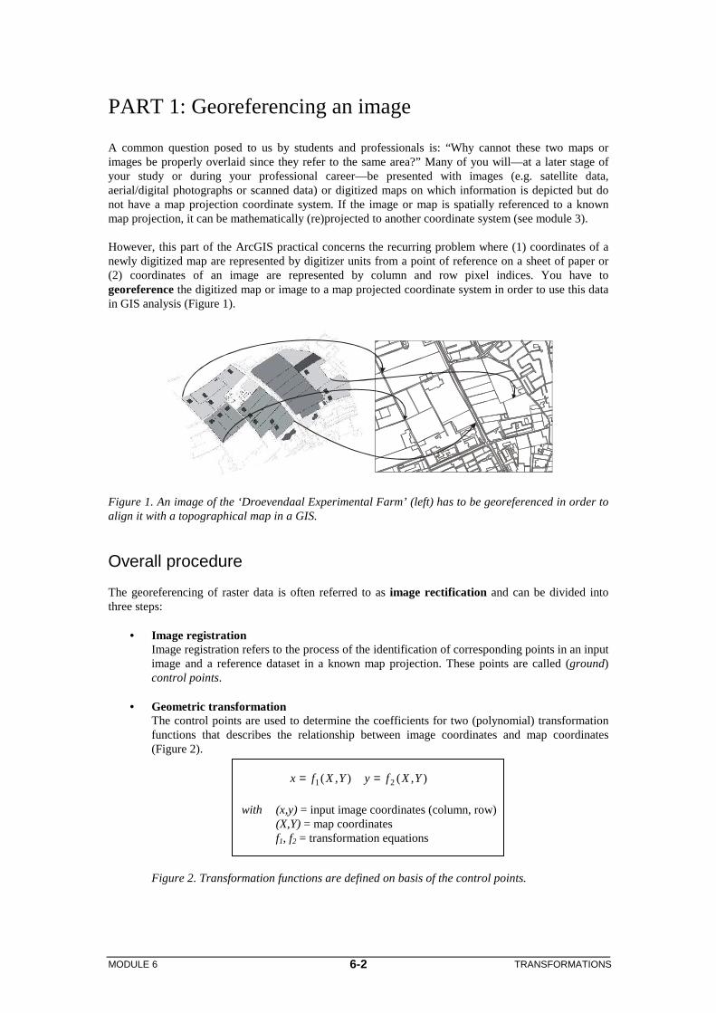
A common question posed to us by students and professionals is: “Why cannot these two maps or images be properly overlaid since they refer to the same area?” Many of you will—at a later stage of your study or during your professional career—be presented with images (e.g. satellite data, aerial/digital photographs or scanned data) or digitized maps on which information is depicted but do not have a map projection coordinate system. If the image or map is spatially referenced to a known map projection, it can be mathematically (re)projected to another coordinate system (see module 3). However, this part of the ArcGIS practical concerns the recurring problem where (1) coordinates of a newly digitized map are represented by digitizer units from a point of reference on a sheet of paper or (2) coordinates of an image are represented by column and row pixel indices. You have to georeference the digitized map or image to a map projected coordinate system in order to use this data in GIS analysis (Figure 1). Figure 1. An image of the ‘Droevendaal Experimental Farm’ (left) has to be georeferenced in order to align it with a topographical map in a GIS.

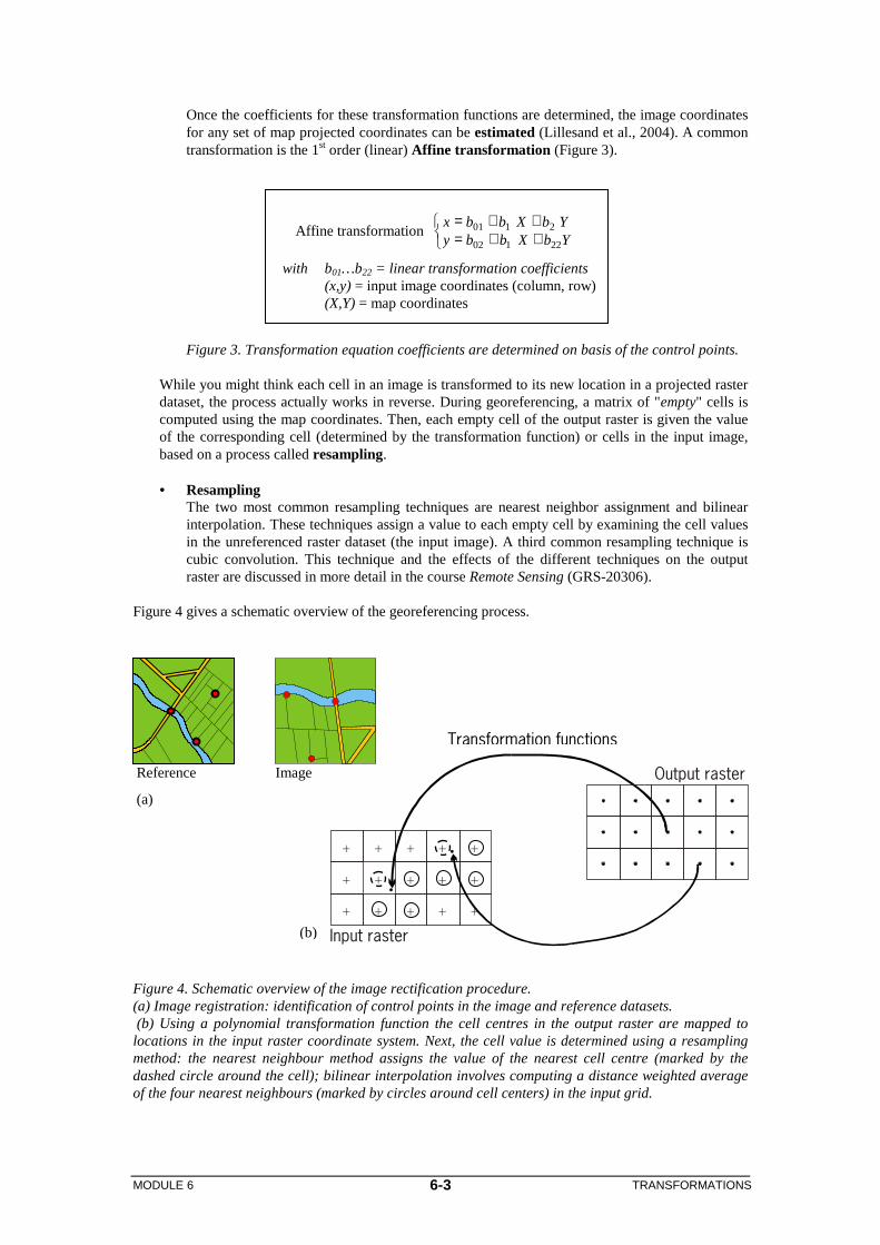
Overall procedure The georeferencing of raster data is often referred to as image rectification and can be divided into three steps:

• Image registration Image registration refers to the process of the identification of corresponding points in an input image and a reference dataset in a known map projection. These points are called (ground) control points.

• Geometric transformation

The control points are used to determine the coefficients for two (polynomial) transformation functions that describes the relationship between image coordinates and map coordinates (Figure 2).

Figure 2. Transformation functions are defined on basis of the control points.

),(),( 21 YXfyYXfx ==

with (x,y) = input image coordinates (column, row) (X,Y) = map coordinates f1, f2 = transformation equations


Once the coefficients for these transformation functions are determined, the image coordinates for any set of map projected coordinates can be estimated (Lillesand et al., 2004). A common transformation is the 1st order (linear) Affine transformation (Figure 3).

Figure 3. Transformation equation coefficients are determined on basis of the control points.

While you might think each cell in an image is transformed to its new location in a projected raster dataset, the process actually works in reverse. During georeferencing, a matrix of "empty" cells is computed using the map coordinates. Then, each empty cell of the output raster is given the value of the corresponding cell (determined by the transformation function) or cells in the input image, based on a process called resampling. • Resampling

The two most common resampling techniques are nearest neighbor assignment and bilinear interpolation. These techniques assign a value to each empty cell by examining the cell values in the unreferenced raster dataset (the input image). A third common resampling technique is cubic convolution. This technique and the effects of the different techniques on the output raster are discussed in more detail in the course Remote Sensing (GRS-20306).

Figure 4 gives a schematic overview of the georeferencing process.

Figure 4. Schematic overview of the image rectification procedure. (a) Image registration: identification of control points in the image and reference datasets. (b) Using a polynomial transformation function the cell centres in the output raster are mapped to locations in the input raster coordinate system. Next, the cell value is determined using a resampling method: the nearest neighbour method assigns the value of the nearest cell centre (marked by the dashed circle around the cell); bilinear interpolation involves computing a distance weighted average of the four nearest neighbours (marked by circles around cell centers) in the input grid.

+

+

+

+

+

+

+

+

+

+

+

+

+

+

+

Transformation functions

Output raster

Input raster

(a)

(b)

Reference Image

with b01…b22 = linear transformation coefficients (x,y) = input image coordinates (column, row) (X,Y) = map coordinates

+ + = + + =

Y b X b b y Y b X b b x

22 1

02 2

1

01 Affine transformation


Georeferencing in ArcMap In this module you will georeference an image of the ‘Droevendaal Experimental Farm’ from image coordinates to projected map coordinates. 1. Open ArcMap document ‘Transformations part1.mxd’. Activate data frame ‘Scanned image’. This data frame contains an image of the ‘Droevendaal Experimental Farm’. a. What is a nominal data scale? How do you know that the values of raster layer ‘Scanned map’ are on nominal scale? b. What is the unit of the coordinates of the scanned image coordinates (meters or pixels)? How many rows and columns does the image have? c. Add vector layer ‘Top10vct.lyr’ to the data frame. This layer can be found in the data folder. Image registration: obtaining control points You start the georeferencing by obtaining coordinates of control points. These are points where both image and map coordinates can be identified (Chang, 2006). INSTRUCTIONS:

1. Open the Georeferencing toolbar. Click View in the menu bar, point to Toolbars and click Georeferencing.

Figure 5. The Georeferencing toolbar.

2. In the table of contents, right-click the referenced dataset (in this case the ‘Top10vct’) and click Zoom to Layer.

3. Click the Georeferencing dropdown arrow in the Georeferencing toolbar, click Fit to display. Make sure the layer box is set to “scanmap”.

4. Now both layers are displayed in the view window.

1 2


5. Click the Control points tool (box 1, Figure 5). The pointer on the display changes into a

crosshair. 6. To add a control point, click the mouse pointer on a location in the raster dataset which can be

easily recognized in the reference dataset (e.g. a crossing of roads, Figure 6). You will need to zoom in considerably to obtain accurate x, y positions. When collecting control points, first click the source (unreferenced raster) dataset, then click the coinciding point in the referenced dataset.

Figure 6. Collecting control points. A detail of the image and reference datasets showing a control point that links an identical locations in image (top) and reference (bottom) datasets.

7. Collect sufficient control points to solve the transformation equations:

• 1st order polynomial (affine): minimal 3 control points; • 2nd order polynomial: minimal 6 control points; • 3rd order polynomial: minimal 10 control points. However, it is wise to collect more than the required minimum. With more control points coefficient estimations are improved which results in smaller measurement errors and a higher accuracy!!

8. The image and map coordinates of the control points are stored in the Link Table (Figure 7). Click the View Link Table button (box 2, Figure 5). The table shows the x and y coordinates of the control points and the residuals (errors). Make sure the Auto Adjust box is checked.

9. To delete a control point, select it and click the delete button on the upper right hand of the dialog box.

Figure 7. The Link Table with 12 control points. The RMS error is for these 12 points 2.78. The map shows the distribution of the control points.


2. a. What are control points and where do you need them for? b. What are residuals and how are they calculated? Start collecting control points. Answer exercises c and d when you have collected 2 and 4 points, respectively. Collect 12 control points in total. Note that during the collection, the scanned map is adjusted (based on the transformation function) to match the reference dataset after each collected point. Make sure your points are well distributed among the map. c. When you have collected 2 points, open the Link Table. Are there already any residuals calculated. Why (not)? d. Open the table again when you have collected 4 points. What is the Total RMS error (Figure 7)? e. What Total RMS error did you achieve after the collection of the 12 control points? A Total RMS error between 2 and 4 is acceptable. Save the set of control points (open the Link Table and click Save). Place the file in your workspace! f. Replace control points with high residuals if necessary. What happens with the Total RMS error if such control points are removed? g. What does a low RMS value indicate; does it imply an accurate registration and hence good rectification results? Why (not)?


Geometric transformation and resampling Until now you have registered the input image with the reference dataset by obtaining twelve control points. These points were used to fit a transformation function (i.e. determine the coefficients) to the coordinate values of the control points. For each point the residual was calculated which is the difference between fitted coordinate value and the ‘true’ coordinate value of that point. Now you will perform the geometric transformation and resampling of the input image. In ArcGIS these two steps are integrated into one operation! INSTRUCTIONS:

1. First select the transformation function. Click the Georeferencing dropdown arrow in the toolbar, point to Transformation and select a transformation polynomial.

2. Click the Georeferencing dropdown arrow and click Rectify. A dialog box opens (Figure 8). 3. Set the Cell Size for the output raster dataset. 4. Select a Resample Type. 5. And specify the name and location of the output raster. 6. Set format to GRID 7. Click Save.

Figure 8. Enter the rectification settings. 3. Rectify the input image of the experimental farm. Use a 1st order polynomial (Affine) transformation function. Use both the Nearest Neighbor and the Bilinear Interpolation resampling types. Name the output rasters ‘farm_1st_nn’ and ‘farm_1st_bl, respectively. Save the output rasters in your workspace. Change the cell size to 2 meters and set the format to GRID. a. What is the meaning of the Nearest Neighbor and Bilinear resampling type options? Activate data frame ‘Referenced image’ and add both output rasters to it. Change the symbology of the two raster datasets. Open the Symbology editor and import farm.lyr b. Which of the two is correct and why?


4. Add layer ‘top10vct.lyr’ to data frame ‘Referenced image’. a. What pattern in the displacements between the rectified images and the ‘top10vct’ layer can be observed? Hint: zoom in. 5. Activate data frame ‘Scanned image’. Repeat the rectification using a 2nd order transformation function. Name the output raster ‘farm_2nd’. Choose the appropriate resampling type. a. Open the Link Table. What Total RMS error have you achieved now? Activate data frame ‘Referenced image’ and add dataset ‘farm_2nd’. b. Did the spatial match between the rectified image and the reference layer ‘top10vct’ improve? c. How does this result relate to your answer to exercise 5a? Is there any reason to use a 2nd order (quadratic) transformation function?


Validation A low RMS error should not be confused with an accurate rectification. For example, using the minimum number of control points required by the used transformation function, zero RMS should be given. Nevertheless, the transformation may contain substantial errors due to a poorly entered control point. In fact, the RMS only indicates how well the transformation function could be calibrated to the control points. A validation with an independent set of reference points allows checking the positional accuracy obtained. Using a precision instrument (Real Time Kinematic GPS) the locations of corner points of specific experimental plots inside the farm were measured (with centimeter accuracy). These locations were subsequently projected to the Dutch Grid (RD reference system). Figure 9 identifies 15 of the measured locations (north-east corners). Their coordinates (Dutch Grid) are stored in the MS Excel file ‘Validate.xls’.

Figure 9. Fifteen validation locations, the north-east corners of experimental plots.

6. Validate the georeferenced images. Follow the following procedure: 1. Open the Excel workbook ‘Validate.xls’. This file can be found in folder

D:\IGI\...*…\ArcGIS\data\georeferencing (*morning or afternoon). 2. Measure the 15 coordinates of the northeast corner of the validation plots in the map “farm_2nd“.

Use the identify tool and make sure the correct layer (i.e. Farm_2nd) is selected in “the identify from” box. The coordinates are given in the “Location” box

3. Fill in the coordinates in the columns X_image and Y_image of the Excel sheet. 4. The RMS E(rror) of the residuals is automatically computed. 5. Repeat the measurements and calculations with the raster dataset ‘Farm_1st_nn’. a. What overall RMS error did you achieve for the 1st and 2nd order polynominal transformations (give unit)? b. How does this compare to your answer(s) to exercises 5a and if applicable 2d? c. Which factors contribute to the positional accuracy achieved?


Part 2: Dataset structure transformation

The second part of this module deals with the transformation of one dataset structure to another dataset structure: vector data to raster data conversion (called rasterization) and raster data to vector data conversion (called vectorization).

Transforming datasets from vector to raster In vector-vector and raster-raster transformations the geometric elements of the datasets remain the same. In a vector-raster transformation you are confronted with a change in geometric elements. Point, line or polygon features are converted into raster cells. Weight tables to determine the cell value after transformation Transforming vector geometric elements into raster cells force the user to formulate decision rules concerning the attribute value that has to be stored in a specific raster cell. For example, when two line elements intersect in the area of a raster cell which line value will be labeled to the cell? 7. a. Draw a situation showing that it is necessary to make decisions about the value labeling of raster

cells, when transforming: 1. point features to raster cells; 2. polygon features to raster cells. Sketch 1: Sketch 2: In most GIS systems, the user is able to influence the outcome of a decision in case of ambiguity (multiple vector features in one raster cell). A common used approach to define a decision rule is by means of a weight table. These weights are used to resolve cases when a single cell contains more than one vector element. In this case the vector elements with the highest value in the weight value will be assigned to this cell.


8.

The following wells are stored in a vector data-set (Figure 10): 1. wells with good drinking-water quality 2. wells with reasonable drinking-water quality; the water is suitable for livestock consumption 3. wells with poor drinking-water quality; this water will create illness but it is not fatal to humans or

livestock 4. wells with toxic chemicals; this water is fatal for humans and livestock As a remark, in this example it is important to know which the wells with toxic drinking water are. For further analysis, the point elements have to be converted to raster cells. a. Which data scale do the descriptions of the wells have? b. Write down the relation between the above mentioned descriptions about wells by giving it a value

and a weight. The weight value has to ensure that the worst water quality is represented in a raster cell after transformation.

c. During the vector-raster transformation, the coordinates which describe the position of a geometric

element disappear. Describe in your own words what the reason is that this happens. Use your lecture book to support your answer.

d. In the figure below, a raster is draped on the points of the wells described earlier. Fill in the empty

raster at the right with the code number of the well which is assigned to the raster cell according to your weight table given.

Figure 10. Wells described in a vector structure as point elements, with a raster along those points (left) and an empty raster (right).


9. In the next example line objects have to be transformed into a raster environment (Figure 11). The line objects represent different types of roads. The road with the highest traffic capacity is the most important for further analysis, so it has the highest weight value. a. Fill in the empty raster presented below with codes for the different road types according to their

traffic intensity.

Figure 11. Roads described in a vector structure as line elements, with a raster along those lines (left) and an empty raster (right).


10. In the next example polygon objects have to be transformed into a raster environment (Figure 12). More than one polygon object is able to share the area of a raster cell. Many GIS systems determine which partial area is the largest in the cell. The value of this area object will be stored in the raster cell. This means that very small polygons, which are situated completely within a raster cell, are lost. These areas could be very important to the user. Once again a weight table is used as a rule of decision to make sure that this information is not lost. In the example presented below, heather areas play the most important role for future analysis. a. Fill the empty raster with a code number, make sure that all heather areas maintain in the final result.

Figure 12. Land use described in a vector structure as polygon elements, with a raster draped on the polygons and an empty raster.

Vector-raster transformation in ArcMap In ArcMap, any type of feature dataset created from any type of source file can be converted to a raster dataset. Only the selected features in a vector dataset will be converted to raster. If the vector dataset does not contain a selected set, then all features will be converted to a raster dataset. All GIS programs have default decision rules settings. The most common rules are now discussed. When you convert polygons to raster cells, cells are given the value of the polygon with the largest area within the raster cell. During transformations of line features, cells are given the value of the line feature that is found within each cell. When more than one line feature intersects a raster cell, the first line feature value that is encountered during processing is given to the cell. Cells that are not intersected by a line feature are given the value of NoData. When you convert point features, cells are given the value of the point that is found within each cell. If more than point is found in a cell, then the cell is given the value of the point it first encounters when processing. Cells that do not contain a point feature are given the value of NoData. It is important to realize that all raster cells get a value after the transformation from vector. This can either be a value based on the vector feature or the NoData value if the raster cell does not intersect with a vector feature. There will be no empty cells in a raster.


INSTRUCTIONS:

1. Activate the data frame that contains the vector dataset you want to convert to raster 2. Open ArcToolbox; select Conversion Tools � to Raster � Feature to Raster 3. In the dialog box, define the input dataset, the field which will be used to assign the values to

the raster, the output dataset (select a proper location) and the cell size. Click OK. 11. Activate the data frame ‘Wag_south’ of ArcMap document ‘Transformations part2.mxd’. Convert the features of dataset ‘Soil_types’ into raster cells. The cell size of the new raster dataset ‘Soilraster1’ has to be 100 m. For cell values choose field ‘Soilcode’. Store dataset ‘Soilraster1’ in your workspace directory. a. Overlay ‘Soil_types’ with ‘Soilraster1’. Explain why some parts of the polygon features are not

given a cell value based on the soil code (e.g. along the borders of the river Rhine). b. Which value has the highest number of cells? What is the total number of raster cells?

c. Select the Identify tool and click in the Rhine. Are these cells as empty as they appear in the map? Or do they also have a value?

d. Give the cells with the value of NoData a color. Open the Layer properties (double-click the layer).

In the lower right corner of the Symbology tab there is the Display NoData as dropdown list. Click on the arrow and select a color. Explain what happens.

e. How is the raster extent (the raster borders) determined? f. The total number of raster cells you calculated earlier, is the number of raster cells that have a value

based on the attribute ‘Soil code’. Calculate the total number of raster cells again, taking into account the cells with value NoData. Hint: you can find the number of rows and columns of the raster in the Layer properties. Open the layer properties window and select the Source tab.

Convert the features of dataset ‘Soil_types’ to raster cells again, but now the cell size of the new raster dataset ‘Soilraster2’ has to be 10 m. g. Which value has the highest number of cells? What is its total number of raster cells (including the

NoData cells)? h. Which of the two vector-raster transformations gives the best results? Explain your answer.


Transforming datasets from raster to vector The procedure of a raster-vector transformation is the following: 1. Determine the raster cells that form a feature; 2. Determine the edges between the features when necessary. If point features are the final result, this

step is not needed. 12. Determine the individual features in Figure 13. Give each new feature a new identifier number in the empty raster. a. How many new area objects have you determined? Number of objects with value 1: Number of objects with value 2:

Raster-vector transformation in ArcMap If the raster dataset does not contain selected cells, then all the cells will be converted to a vector feature type. In this module only the raster to polygon feature transformation is discussed. The output polygon feature dataset will contain a field called ‘Gridcode’. This field will hold the value of the raster cells used to create the polygon. When the simplify polygons option is used, the polygons in the output feature dataset are smoothed using a cluster tolerance. The cluster tolerance is found in the ‘General Settings’ in the analysis ‘Environments’. If no value is given a program default cluster value is used. INSTRUCTIONS:

1. Activate the data frame that contains the raster dataset you want to convert to vector. 2. Open ArcToolbox; select Conversion Tools � From Raster � Raster to polygon. 3. In the dialog box, define the input dataset, the field which will be used to assign the values to

the vector dataset, the output dataset (select a proper location). Click OK.

Figure 13. Land use described in a raster structure (left) and an empty raster (right).


13. Convert raster dataset ‘Soilraster1’ into the polygon feature dataset ‘Soilvector1’. Dataset ‘Soilvector1’ has to be stored in your workspace directory. Choose the field ‘Soilcode’ to be used in the transformation. a. What are the field names of the attribute table ‘Soilvector1’? b. What are the differences between the attribute table of dataset ‘Soilvector1’ and the attribute

table of the original dataset ‘Soil_types’? c. Where are the biggest discrepancies located in comparison to the original dataset ‘Soil_types’? d. Write down, in your own words, the raster-vector conversion process. 14. Convert raster dataset ‘Soilraster2’ into the polygon feature dataset ‘Soilvector2’. Dataset ‘Soilvector2’ has to be stored in your workspace directory. a. What are the major differences between datasets ‘Soilvector1’ and ‘Soilvector2’, and between

datasets ‘Soilvector2’ and ‘Soil_types’? Explain these differences. b. Where are the biggest discrepancies between datasets ‘Soilvector2’ and ‘Soil_types’? Changing the cell size of a raster dataset If you want to compare rasters, they have to have the same cell size. However there are some pitfalls when changing the raster cell size.

1. If you decrease the cell size (e.g. from 30 m to 10 m) the spatial accuracy does not increase, since the source data had a cellsize of 30 x 30 m.(See Figure 14a)

2. If you increase the cell size you will encounter similar problems as in Part I of this module. You will have to use a resampling technique (nearest neighbor, bilinear interpolation). (See Figure 14b)

3. In both cases you can also encounter geometric shift of the data if your two cellsizes do not fit in each other. If you go from 30 x 30 m cells to 10x10 m cells, exactly 9 news cells with similar values will be created at the original postion of one 30x30 cell. However if you go from 30x30 cells to 20x20 cells your new cells boundaries won’t coincide with your old cell boundaries. In these cases the resampling method again is of importance. (See Figure 14c)


z

Figure 14. Different resampling options. (a) going to a smaller cell size, without changing the geometric meaning, (b) going to a larger cell size, (c) going to a smaller cell size and changing the geometric meaning.

1 2 2

1 1 2

1 2 1

?

1

2

2

1

1 1 1

1 1 1

1 1 1

2 2 2

2 2 2

2 2 2

2 2 2

2 2 2

2 2 2

1 1 1

1 1 1

1 1 1

a

b

1

2

2

1

c

1

?

2

?

?

?

2

?

1


INSTRUCTIONS

1. Open ArcToolbox, go to Data Management Tools�Raster�Raster Processing� Resample 2. Select your input raster 3. Define a name for the output raster 4. Define the new Cell Size 5. Select a resampling technique (default is nearest neighbour) 6. Click OK

15. a. Convert soilraster1 to a dataset soilraster3 this time with a cell size of 50m with the nearest

neighbor resampling technique. Is the new raster dataset geometrically different and more accurate? b. Convert soilraster1 to a dataset soilraster4, this time with a cell size of 30m with the nearest

neighbor resampling technique. Is the new raster dataset geometrically different and more accurate? c. Should you use the bilinear resampling technique for transforming the soilraster dataset? Explain

your answer. d. Suppose you have to compare to land use rasters, one from 1950 (with a cell size of 50m) and one

from 2000 (30m) which cell size and resampling technique will you use for your analysis?

Documents

Module 6 Transformations 20-08-2010scomp5063.wur.nl/courses/grs10306/Materials/Practical/1... · 2010-11-04 · 6. TRANSFORMATIONS 6-1 INTRODUCTION 6-1 ... The two most common resampling