Jisy Raju Asst.Professor, CSE

CE, Cherthala

Module 4 Relational Database Design: Different anomalies in designing a database, normalization, functional dependency (FD), Armstrong’s Axioms, closures, Equivalence of FDs, minimal Cover (proofs not required). Normalization using functional dependencies, INF, 2NF, 3NF and BCNF, lossless and dependency preserving decompositions

Relational Database Design Relational database design (RDD) models information and data into a set of tables with rows and columns. Each row of a relation/table represents a record, and each column represents an attribute of data. The Structured Query Language (SQL) is used to manipulate relational databases. The design of a relational database is composed of four stages, where the data are modeled into a set of related tables. The stages are:

● Define relations/attributes ● Define primary keys ● Define relationships ● Normalization

4.1 Different anomalies in designing a database Anomalies something that deviates from what is standard, normal, or expect. There are three types of anomalies,

● Insertion Anomalies ● Deletion ● Updation

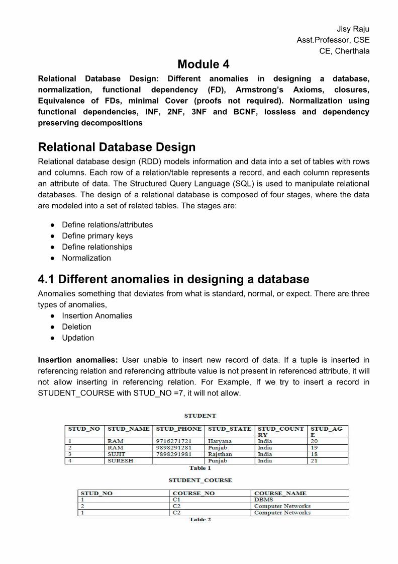
Insertion anomalies: User unable to insert new record of data. If a tuple is inserted in referencing relation and referencing attribute value is not present in referenced attribute, it will not allow inserting in referencing relation. For Example, If we try to insert a record in STUDENT_COURSE with STUD_NO =7, it will not allow.

Deletion Anomalies: Happen when the deletion of unwanted information causes desired information to be deleted as well. We can’t delete a row from REFERENCED RELATION if value of REFRENCED ATTRIBUTE is used in value of REFERENCING ATTRIBUTE.it can be handled by DELETE CASCADE: It will delete the tuples from REFERENCING RELATION if value used by REFERENCING ATTRIBUTE is deleted from REFERENCED RELATION. Updation Anomalies: when a record is updated, but the appearance of same record are not get update.We can’t update a row from REFERENCED RELATION if value of REFRENCED ATTRIBUTE is used in value of REFERENCING ATTRIBUTE. UPDATE CASCADE: It will update the REFERENCING ATTRIBUTE in REFERENCING RELATION if attribute value used by REFERENCING ATTRIBUTE is updated in REFERENCED RELATION.

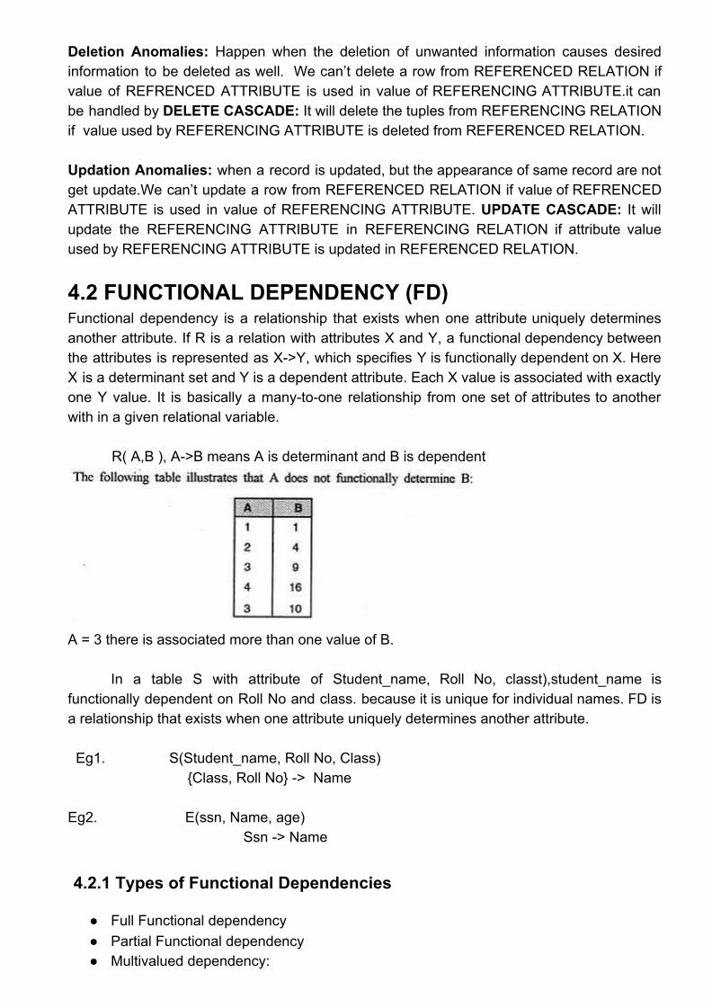
4.2 FUNCTIONAL DEPENDENCY (FD) Functional dependency is a relationship that exists when one attribute uniquely determines another attribute. If R is a relation with attributes X and Y, a functional dependency between the attributes is represented as X->Y, which specifies Y is functionally dependent on X. Here X is a determinant set and Y is a dependent attribute. Each X value is associated with exactly one Y value. It is basically a many-to-one relationship from one set of attributes to another with in a given relational variable. R( A,B ), A->B means A is determinant and B is dependent

A = 3 there is associated more than one value of B.

In a table S with attribute of Student_name, Roll No, classt),student_name is functionally dependent on Roll No and class. because it is unique for individual names. FD is a relationship that exists when one attribute uniquely determines another attribute.

Eg1. S(Student_name, Roll No, Class) {Class, Roll No} -> Name Eg2. E(ssn, Name, age) Ssn -> Name

4.2.1 Types of Functional Dependencies

● Full Functional dependency ● Partial Functional dependency ● Multivalued dependency:

● Trivial functional dependency: ● Non-trivial functional dependency: ● Transitive dependency

Full Functional dependency: A full functional dependency is a functional dependency where the left-hand side is a superkey. A functional dependency X → Y is a full functional dependency if removal of any attribute A from X means that the dependency does not hold any more; In R(A,B,C) if (A,B)->C holds and neither A->C nor B->C holds then it is fully functionally dependent on (A,B). A,B is known as Prime attribute and C is known as Non prime attribute.

Assume a relation S with attribute of Student_name, Roll No, class. The set of attributes Student_name are fully dependent on the attributes (Roll No, class). This means we need to get the information of both Roll No and class to get values of student_name.

Partial Functional dependency: A FD (functional dependency) that holds in a relation is partial when removing one of the determining attributes gives a FD that holds in the relation.

Eg if {A,B} → {C} but also {A} → {C} then {C} is partially functionally dependent on {A,B}.

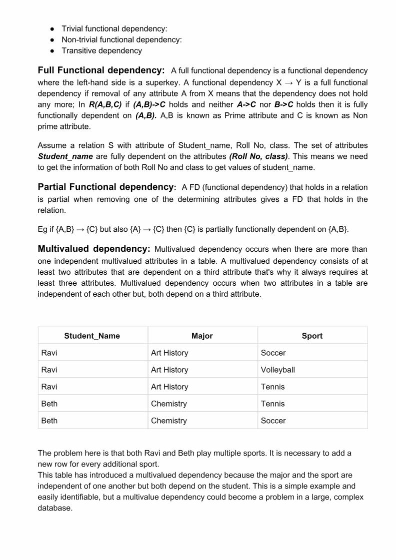
Multivalued dependency: Multivalued dependency occurs when there are more than one independent multivalued attributes in a table. A multivalued dependency consists of at least two attributes that are dependent on a third attribute that's why it always requires at least three attributes. Multivalued dependency occurs when two attributes in a table are independent of each other but, both depend on a third attribute.

Student_Name Major Sport

Ravi Art History Soccer

Ravi Art History Volleyball

Ravi Art History Tennis

Beth Chemistry Tennis

Beth Chemistry Soccer

The problem here is that both Ravi and Beth play multiple sports. It is necessary to add a new row for every additional sport. This table has introduced a multivalued dependency because the major and the sport are independent of one another but both depend on the student. This is a simple example and easily identifiable, but a multivalue dependency could become a problem in a large, complex database.

Trivial functional dependency: If a functional dependency (FD) X → Y holds, where Y is a subset of X, then it is called a trivial FD.

For example: Consider a table with two columns Student_id and Student_Name. {Student_Id, Student_Name} -> Student_Id is a trivial functional dependency as Student_Id is a subset of {Student_Id, Student_Name}.

Non-trivial functional dependency: If a functional dependency X->Y holds true where Y is not a subset of X then this dependency is called non trivial Functional dependency.

For example:An employee table with three attributes: emp_id, emp_name, emp_address.

The following functional dependencies are non-trivial:

emp_id -> emp_name (emp_name is not a subset of emp_id)

{emp_id, emp_name} -> emp_address (emp_address is not a subset of emp_id, emp_name)

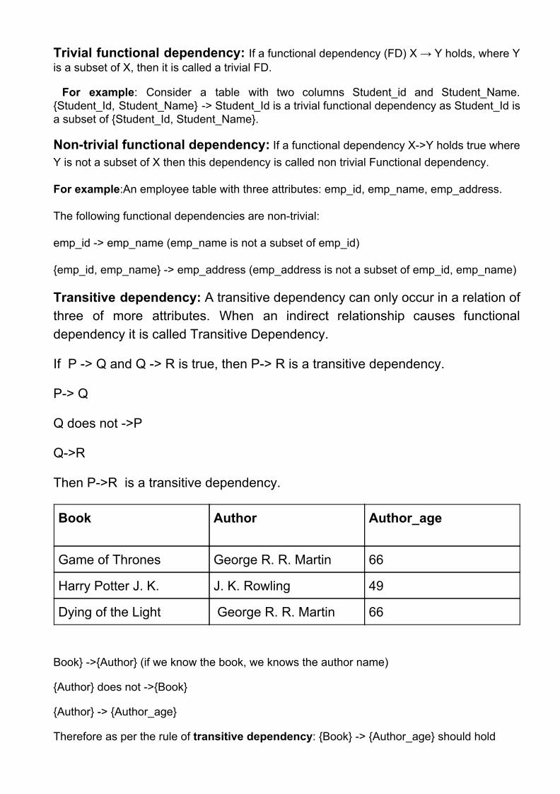
Transitive dependency: A transitive dependency can only occur in a relation of three of more attributes. When an indirect relationship causes functional dependency it is called Transitive Dependency.

If P -> Q and Q -> R is true, then P-> R is a transitive dependency.

P-> Q

Q does not ->P

Q->R

Then P->R is a transitive dependency.

Book Author

Author_age

Game of Thrones George R. R. Martin 66

Harry Potter J. K. J. K. Rowling 49

Dying of the Light George R. R. Martin 66

Book} ->{Author} (if we know the book, we knows the author name)

{Author} does not ->{Book}

{Author} -> {Author_age}

Therefore as per the rule of transitive dependency: {Book} -> {Author_age} should hold

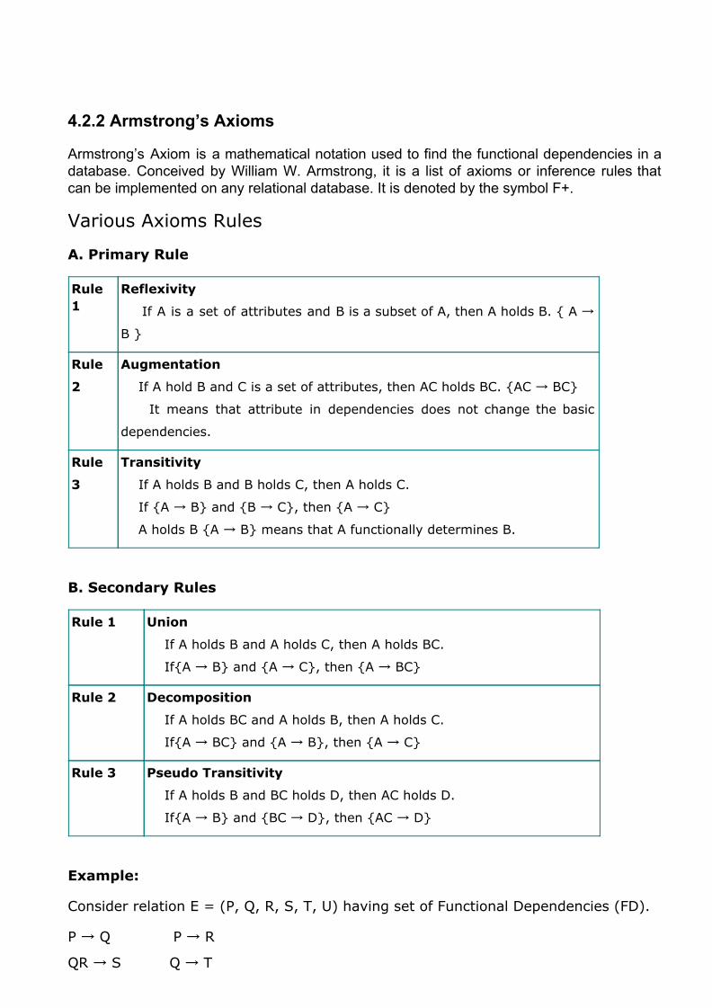
4.2.2 Armstrong’s Axioms

Armstrong’s Axiom is a mathematical notation used to find the functional dependencies in a database. Conceived by William W. Armstrong, it is a list of axioms or inference rules that can be implemented on any relational database. It is denoted by the symbol F+.

Various Axioms Rules

A. Primary Rule

Rule

1

Reflexivity

If A is a set of attributes and B is a subset of A, then A holds B. { A →

B }

Rule

2

Augmentation

If A hold B and C is a set of attributes, then AC holds BC. {AC → BC}

It means that attribute in dependencies does not change the basic

dependencies.

Rule

3

Transitivity

If A holds B and B holds C, then A holds C.

If {A → B} and {B → C}, then {A → C}

A holds B {A → B} means that A functionally determines B.

B. Secondary Rules

Rule 1 Union

If A holds B and A holds C, then A holds BC.

If{A → B} and {A → C}, then {A → BC}

Rule 2 Decomposition

If A holds BC and A holds B, then A holds C.

If{A → BC} and {A → B}, then {A → C}

Rule 3 Pseudo Transitivity

If A holds B and BC holds D, then AC holds D.

If{A → B} and {BC → D}, then {AC → D}

Example:

Consider relation E = (P, Q, R, S, T, U) having set of Functional Dependencies (FD).

P → Q P → R

QR → S Q → T

QR → U PR → U

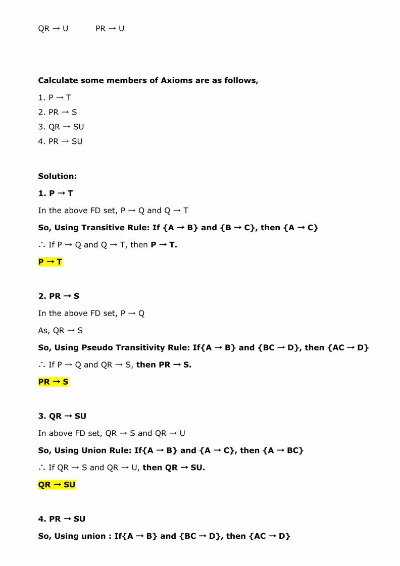
Calculate some members of Axioms are as follows,

1. P → T

2. PR → S

3. QR → SU

4. PR → SU

Solution:

1. P → T

In the above FD set, P → Q and Q → T

So, Using Transitive Rule: If {A → B} and {B → C}, then {A → C}

∴ If P → Q and Q → T, then P → T.

P → T

2. PR → S

In the above FD set, P → Q

As, QR → S

So, Using Pseudo Transitivity Rule: If{A → B} and {BC → D}, then {AC → D}

∴ If P → Q and QR → S, then PR → S.

PR → S

3. QR → SU

In above FD set, QR → S and QR → U

So, Using Union Rule: If{A → B} and {A → C}, then {A → BC}

∴ If QR → S and QR → U, then QR → SU.

QR → SU

4. PR → SU

So, Using union : If{A → B} and {BC → D}, then {AC → D}

∴ If PR → S and PR → U, then PR → SU.

PR → SU

4.2.3 Closure Of Functional Dependency

The Closure Of Functional Dependency means the complete set of all possible attributes that can be functionally derived from given functional dependency

● If “F” is a functional dependency then closure of functional dependency can be denoted using “{F}+”.

● There are three steps to calculate closure of functional dependency. These are:

Step-1 : Add the attributes which are present on Left Hand Side in the original functional dependency.

Step-2 : Now, add the attributes present on the Right Hand Side of the functional dependency.

Step-3 : With the help of attributes present on Right Hand Side, check the other attributes that can be derived from the other given functional dependencies. Repeat this process until all the possible attributes which can be derived are added in the closure.

Closure Of Functional Dependency : Examples

Example-1 : Consider the table student_details having (Roll_No, Name,Marks, Location) as the attributes and having two functional dependencies.

FD1 : Roll_No -> Name, Marks

FD2 : Name -> Marks, Location

Step-1: {Roll_no}+ = {Roll_No}

Step-2 : {Roll_no}+ = {Roll_No,Name, Marks}

Step-3 : {Roll_no}+ = {Roll_No, Marks, Name, Location}

Similarly, we can calculate closure for other attributes too i.e “Name”.

Step-1 : {Name}+ = {Name}

Step-2 : {Name}+ = {Name, Marks, Location}

Step-3 : Since, we don’t have any functional dependency where “Marks or Location”. So

{Name}+ = {Name, Marks, Location}

{Marks}+ = {Marks}

and

{Location}+ = { Location}

Example-2 : Consider a relation R(A,B,C,D,E) having below mentioned functional dependencies.

FD1 : A -> BC

FD2 : C -> B

FD3 : D -> E

FD4 : E -> D

Now, calculate the closure of attributes of the relation R. The closures will be:

{A}+ = {A, B, C}

{B}+ = {B}

{C}+ = {B, C}

{D}+ = {D, E}

{E}+ = {E, D}

Closure Of Functional Dependency : Calculating Candidate Key

A Candidate Key of a relation is an attribute or set of attributes that can determine the whole relation or contains all the attributes in its closure.

Example-1 : Consider the relation R(A,B,C) with given functional dependencies :

FD1 : A-> B

FD2 : B ->C

{A}+ = {A, B, C}

{B}+ = {B, C}

{C}+ = {C} Clearly, “A” is the candidate key as, its closure contains all the attributes present in the relation “R”.

Example-2 : Consider another relation R(A, B, C, D, E) having the Functional dependencies :

FD1 : A-> BC

FD2 : C-> B

FD3 : D ->E

FD4 : E ->D

{A}+ = {A, B, C}

{B}+ = {B}

{C}+ = {C, B}

{D}+ = {E, D}

{E}+ = {E, D} In this case, a single attribute does is unable to determine all the attribute on its own like in previous example. Here, we need to club two or more attributes to determine the candidate keys.

{A, D}+ = {A, B, C, D, E}

{A, E}+ = {A, B, C, D, E}

Hence, "AD" and "AE" are the two possible keys of the given relation “R”. Any other combination other than these two would have acted as extraneous attributes.

Closure Of Functional Dependency : Key Definitions

1. Prime Attributes : Attributes which are indispensable part of candidate keys. For example : “A, D, E” attributes are prime attributes in above example-2.

2. Non-Prime Attributes : Attributes other than prime attributes which does not take part in formation of candidate keys. For example.

3. Extraneous Attributes : Attributes which does not make any effect on removal from candidate key.

For example : Consider the relation R(A, B, C, D) with functional dependencies :

FD1 : A-> BC

FD2 : B ->C

FD3 : D ->C

Here, Candidate key can be “AD” only. Hence,

Prime Attributes : A, D.

Non-Prime Attributes : B, C

Extraneous Attributes : B, C(As if we add any of the to the candidate key, it will remain unaffected). Those attributes, which if removed does not affect closure of that set.

4.3 Equivalence of Functional Dependencies Two different sets of functional dependencies for a given relation may or may not be equivalent. If FD1 and FD2 are the two sets of functional dependencies following with below 3 cases are possible, then FD’s are equivalent.

● If FD1 can be derived from FD2, we can say that FD2 ⊃ FD1.

● If FD2 can be derived from FD1, we can say that FD1 ⊃ FD2.

● If above two cases are true, FD1=FD2.

Q. Let us take an example to show the relationship between two FD sets. A relation

R(A,B,C,D) having two FD sets FD1 = {A->B, B->C, AB->D} and FD2 = {A->B, B->C,

A->C, A->D}

Step 1. Checking whether all FDs of FD1 are present in FD2

● A->B in set FD1 is present in set FD2.

● B->C in set FD1 is also present in set FD2.

● AB->D in present in set FD1 but not directly in FD2 but we will check whether we

can derive it or not. For set FD2, (AB)+ = {A,B,C,D}. It means that AB can

functionally determine A, B, C and D. So AB->D will also hold in set FD2.

As all FDs in set FD1 also hold in set FD2, FD2 ⊃ FD1 is true.

Step 2. Checking whether all FDs of FD2 are present in FD1

● A->B in set FD2 is present in set FD1.

● B->C in set FD2 is also present in set FD1.

● A->C is present in FD2 but not directly in FD1 but we will check whether we can

derive it or not. For set FD1, (A)+ = {A,B,C,D}. It means that A can functionally

determine A, B, C and D. SO A->C will also hold in set FD1.

● A->D is present in FD2 but not directly in FD1 but we will check whether we can

derive it or not. For set FD1, (A)+ = {A,B,C,D}. It means that A can functionally

determine A, B, C and D. SO A->D will also hold in set FD1.

As all FDs in set FD2 also hold in set FD1, FD1 ⊃ FD2 is true.

Step 3. As FD2 ⊃ FD1 and FD1 ⊃ FD2 both are true FD2 =FD1 is true. These two FD sets

are semantically equivalent.

Q. Let us take another example to show the relationship between two FD sets. A

relation R2(A,B,C,D) having two FD sets FD1 = {A->B, B->C,A->C} and FD2 = {A->B,

B->C, A->D}

Step 1. Checking whether all FDs of FD1 are present in FD2

● A->B in set FD1 is present in set FD2. ● B->C in set FD1 is also present in set FD2. ● A->C is present in FD1 but not directly in FD2 but we will check whether we can

derive it or not. For set FD2, (A)+ = {A,B,C,D}. It means that A can functionally determine A, B, C and D. SO A->C will also hold in set FD2.

As all FDs in set FD1 also hold in set FD2, FD2 ⊃ FD1 is true.

Step 2. Checking whether all FDs of FD2 are present in FD1

● A->B in set FD2 is present in set FD1. ● B->C in set FD2 is also present in set FD1. ● A->D is present in FD2 but not directly in FD1 but we will check whether we can

derive it or not. For set FD1, (A)+ = {A,B,C}. It means that A can’t functionally determine D. SO A->D will not hold in FD1.

As all FDs in set FD2 do not hold in set FD1, FD2 ⊄ FD1.

Step 3. In this case, FD2 ⊃ FD1 and FD2 ⊄ FD1, these two FD sets are not semantically equivalent.

4.4 Minimal Cover

Whenever a user updates the database, the system must check whether any of the functional dependencies are getting violated in this process. If there is a violation of dependencies in the new database state, the system must roll back. Working with a huge set of functional dependencies can cause unnecessary added computational time. This is where the minimal cover comes into play.

There are 4 rules to find Minimal cover :

1. Break down the RHS of each functional dependency into a single attribute . 2. Find redundant fds 3. Minimize LHS. 4. Group the functional dependencies that have common LHS together into a Single FD .

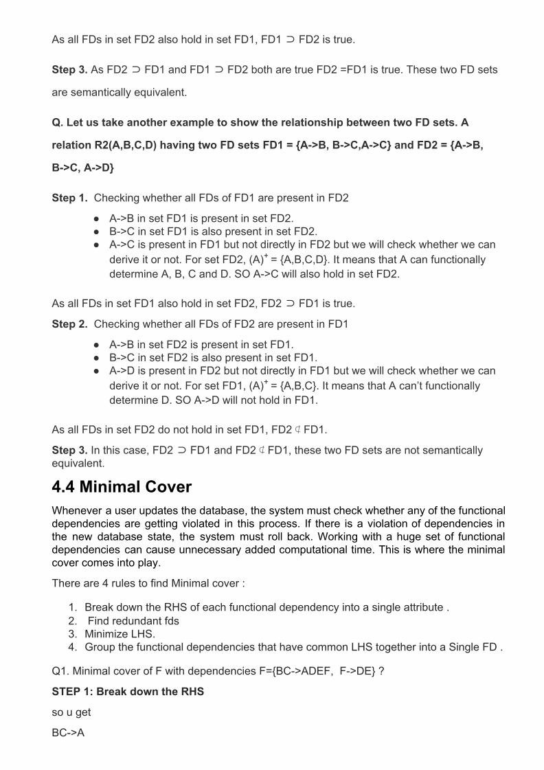
Q1. Minimal cover of F with dependencies F={BC->ADEF, F->DE} ?

STEP 1: Break down the RHS

so u get

BC->A

BC->D

BC->E

BC->F

F->D

F->E

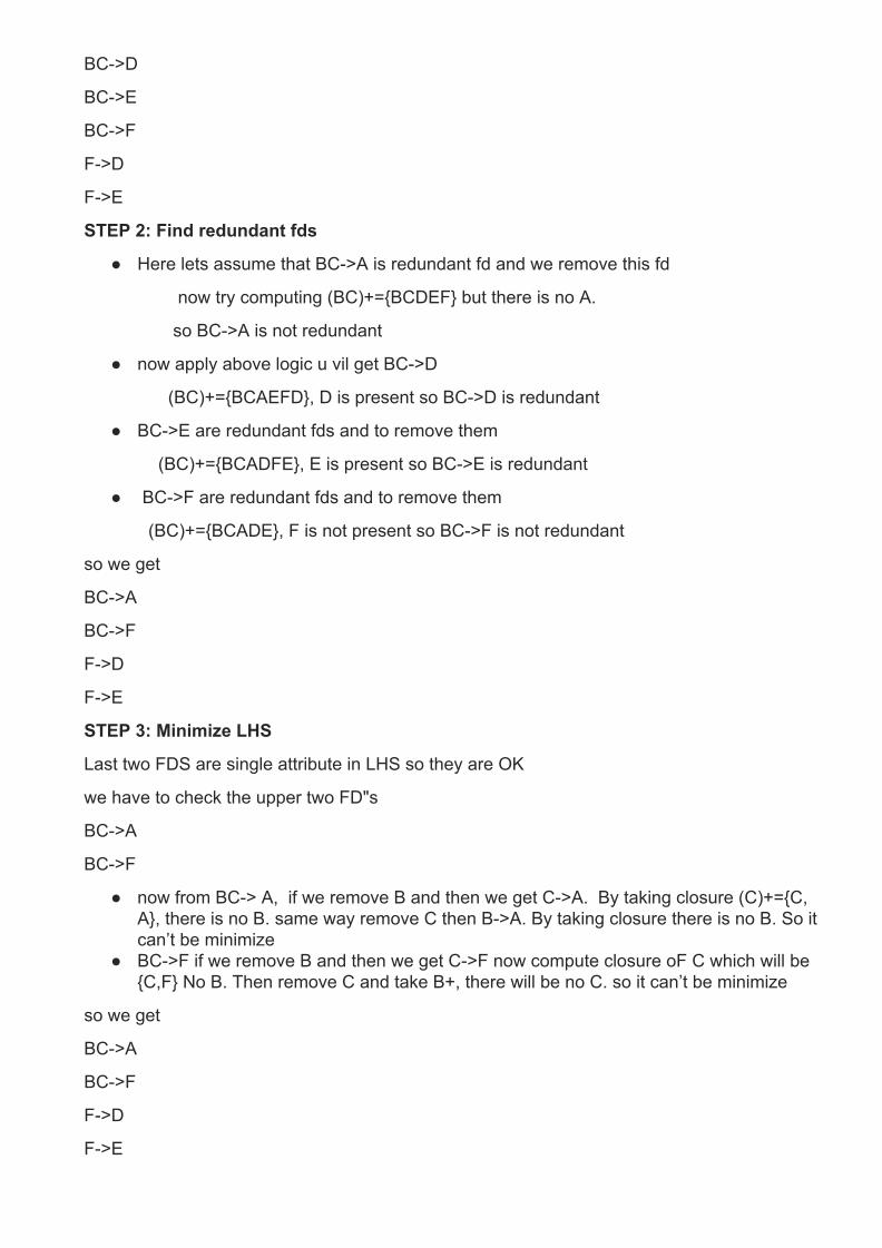
STEP 2: Find redundant fds

● Here lets assume that BC->A is redundant fd and we remove this fd

now try computing (BC)+={BCDEF} but there is no A.

so BC->A is not redundant

● now apply above logic u vil get BC->D

(BC)+={BCAEFD}, D is present so BC->D is redundant

● BC->E are redundant fds and to remove them

(BC)+={BCADFE}, E is present so BC->E is redundant

● BC->F are redundant fds and to remove them

(BC)+={BCADE}, F is not present so BC->F is not redundant

so we get

BC->A

BC->F

F->D

F->E

STEP 3: Minimize LHS

Last two FDS are single attribute in LHS so they are OK

we have to check the upper two FD"s

BC->A

BC->F

● now from BC-> A, if we remove B and then we get C->A. By taking closure (C)+={C, A}, there is no B. same way remove C then B->A. By taking closure there is no B. So it can’t be minimize

● BC->F if we remove B and then we get C->F now compute closure oF C which will be {C,F} No B. Then remove C and take B+, there will be no C. so it can’t be minimize

so we get

BC->A

BC->F

F->D

F->E

Step 4: Group the functional dependencies that have common LHS together into a Single FD .

so the minimal cover is

BC->A F

F->DE

4.5 Normalization Normalization is the process of organizing the data in the database. Normalization is used to

minimize the redundancy from a relation or set of relations. It is also used to eliminate the undesirable characteristics like Insertion, Update and Deletion Anomalies. Normalization divides the larger table into the smaller table and links them using relationship.

The most commonly used normal forms:

● First normal form(1NF)

● Second normal form(2NF)

● Third normal form(3NF)

● Boyce & Codd normal form (BCNF)

Additionally 4NF and 5NF are there,

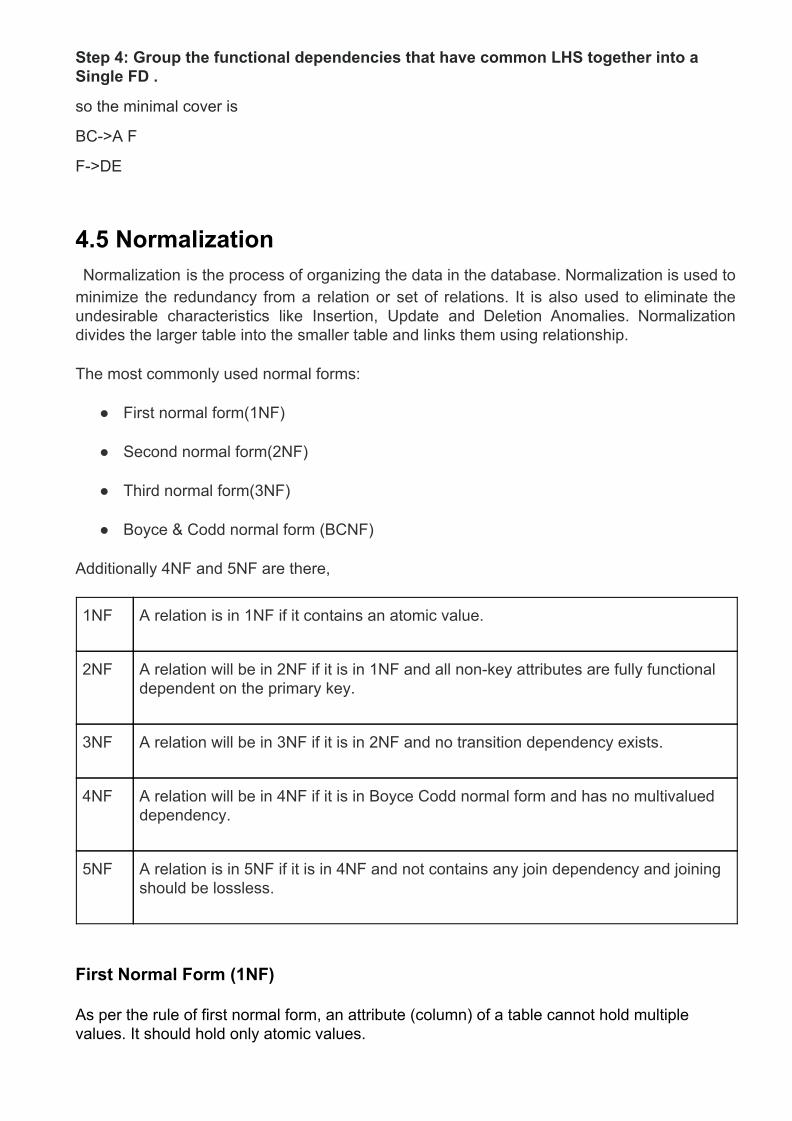
1NF A relation is in 1NF if it contains an atomic value.

2NF A relation will be in 2NF if it is in 1NF and all non-key attributes are fully functional dependent on the primary key.

3NF A relation will be in 3NF if it is in 2NF and no transition dependency exists.

4NF A relation will be in 4NF if it is in Boyce Codd normal form and has no multivalued dependency.

5NF A relation is in 5NF if it is in 4NF and not contains any join dependency and joining should be lossless.

First Normal Form (1NF)

As per the rule of first normal form, an attribute (column) of a table cannot hold multiple values. It should hold only atomic values.

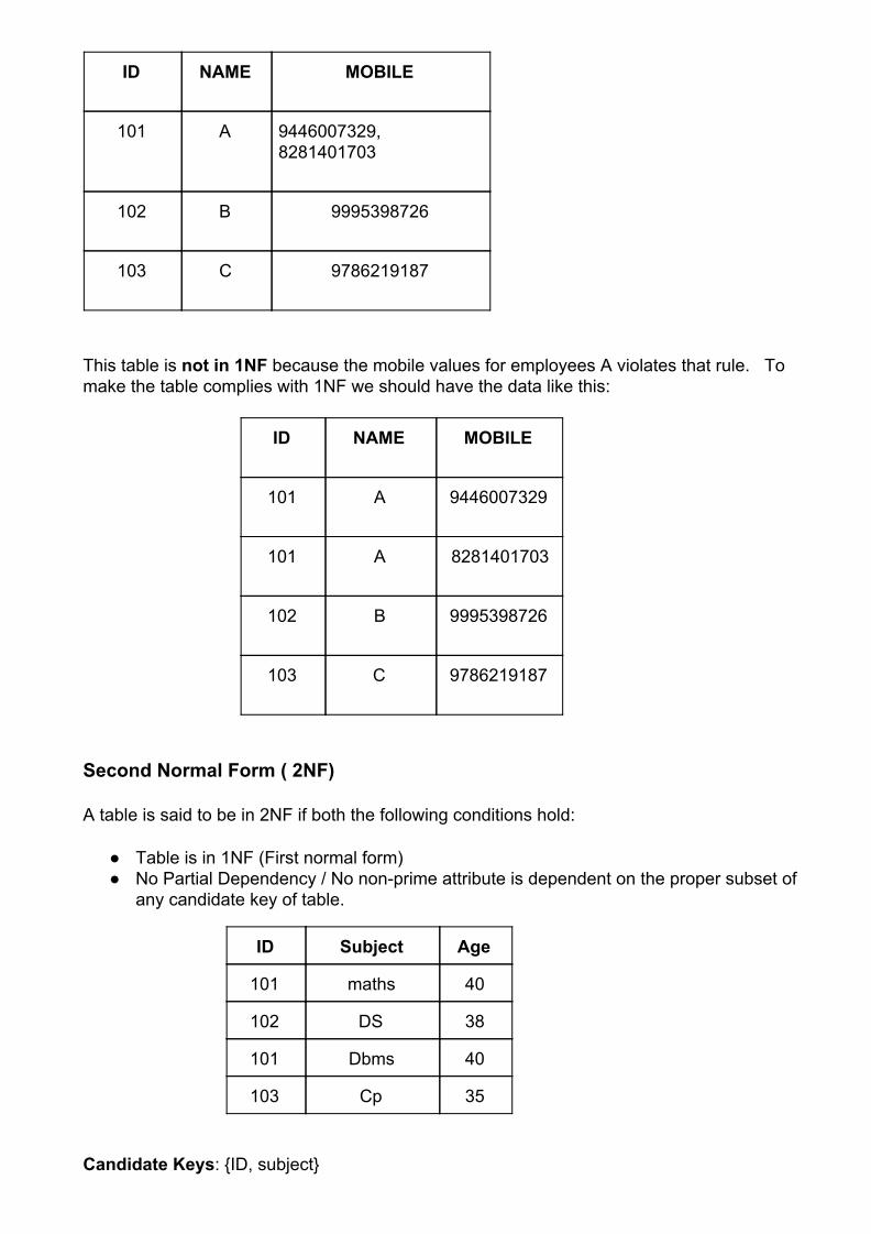
ID NAME MOBILE

101 A 9446007329, 8281401703

102 B 9995398726

103 C 9786219187

This table is not in 1NF because the mobile values for employees A violates that rule. To make the table complies with 1NF we should have the data like this:

ID NAME MOBILE

101 A 9446007329

101 A 8281401703

102 B 9995398726

103 C 9786219187

Second Normal Form ( 2NF)

A table is said to be in 2NF if both the following conditions hold:

● Table is in 1NF (First normal form) ● No Partial Dependency / No non-prime attribute is dependent on the proper subset of

any candidate key of table.

ID Subject Age

101 maths 40

102 DS 38

101 Dbms 40

103 Cp 35

Candidate Keys: {ID, subject}

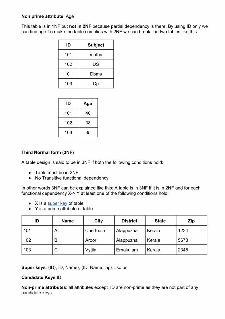
Non prime attribute: Age

This table is in 1NF but not in 2NF because partial dependency is there. By using ID only we can find age.To make the table complies with 2NF we can break it in two tables like this:

ID Subject

101 maths

102 DS

101 Dbms

103 Cp

ID Age

101 40

102 38

103 35

Third Normal form (3NF)

A table design is said to be in 3NF if both the following conditions hold:

● Table must be in 2NF ● No Transitive functional dependency

In other words 3NF can be explained like this: A table is in 3NF if it is in 2NF and for each functional dependency X-> Y at least one of the following conditions hold:

● X is a super key of table ● Y is a prime attribute of table

ID Name City District State Zip

101 A Cherthala Alappuzha Kerala 1234

102 B Aroor Alappuzha Kerala 5678

103 C Vytila Ernakulam Kerala 2345

Super keys: {ID}, ID, Name}, {ID, Name, zip}…so on

Candidate Keys:ID

Non-prime attributes: all attributes except ID are non-prime as they are not part of any candidate keys.

To make this table complies with 3NF we have to break the table into two tables to remove the transitive dependency:

ID Name City Zip

101 A Cherthala 1234

102 B Aroor 5678

103 C Vytila 2345

Zip District State

1234 Alappey Kerala

5678 Alappey Kerala

2345 Ernakulam Kerala

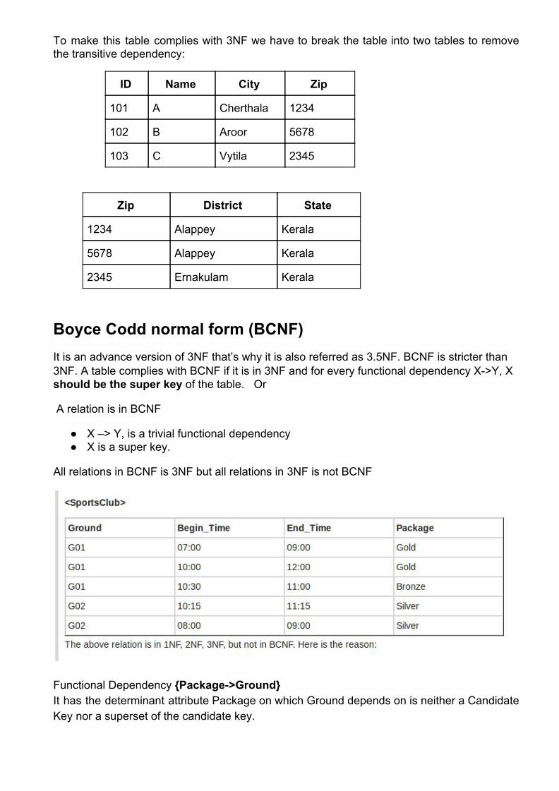
Boyce Codd normal form (BCNF) It is an advance version of 3NF that’s why it is also referred as 3.5NF. BCNF is stricter than 3NF. A table complies with BCNF if it is in 3NF and for every functional dependency X->Y, X should be the super key of the table. Or

A relation is in BCNF

● X –> Y, is a trivial functional dependency ● X is a super key.

All relations in BCNF is 3NF but all relations in 3NF is not BCNF

Functional Dependency {Package->Ground} It has the determinant attribute Package on which Ground depends on is neither a Candidate Key nor a superset of the candidate key.

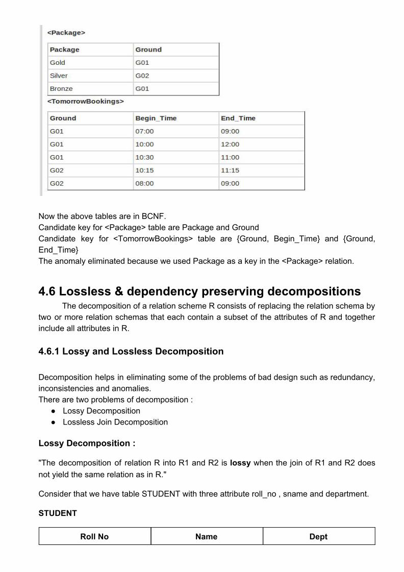
Now the above tables are in BCNF. Candidate key for <Package> table are Package and Ground Candidate key for <TomorrowBookings> table are {Ground, Begin_Time} and {Ground, End_Time} The anomaly eliminated because we used Package as a key in the <Package> relation.

4.6 Lossless & dependency preserving decompositions

The decomposition of a relation scheme R consists of replacing the relation schema by two or more relation schemas that each contain a subset of the attributes of R and together include all attributes in R. 4.6.1 Lossy and Lossless Decomposition Decomposition helps in eliminating some of the problems of bad design such as redundancy, inconsistencies and anomalies. There are two problems of decomposition :

● Lossy Decomposition ● Lossless Join Decomposition

Lossy Decomposition :

"The decomposition of relation R into R1 and R2 is lossy when the join of R1 and R2 does not yield the same relation as in R."

Consider that we have table STUDENT with three attribute roll_no , sname and department.

STUDENT

Roll No Name Dept

11 A CS

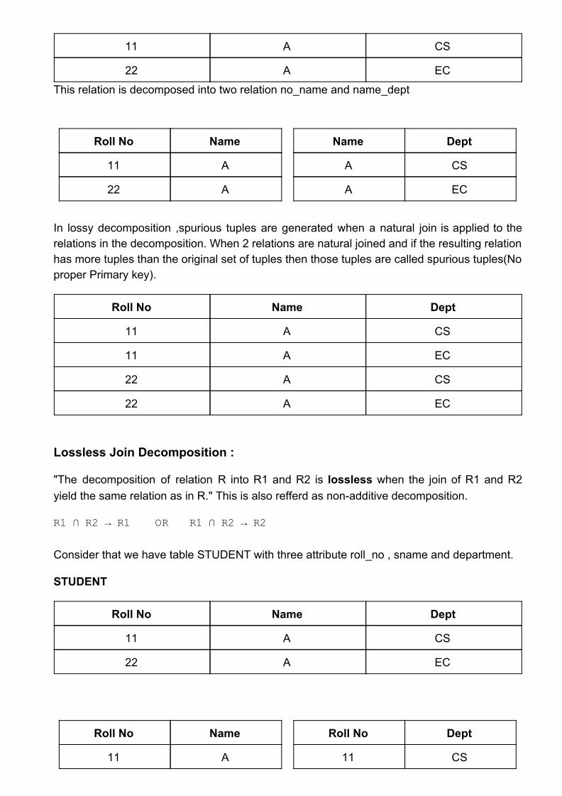
22 A EC This relation is decomposed into two relation no_name and name_dept

Roll No Name

11 A

22 A

Name Dept

A CS

A EC

In lossy decomposition ,spurious tuples are generated when a natural join is applied to the relations in the decomposition. When 2 relations are natural joined and if the resulting relation has more tuples than the original set of tuples then those tuples are called spurious tuples(No proper Primary key).

Roll No Name Dept

11 A CS

11 A EC

22 A CS

22 A EC

Lossless Join Decomposition :

"The decomposition of relation R into R1 and R2 is lossless when the join of R1 and R2 yield the same relation as in R." This is also refferd as non-additive decomposition.

R1 ∩ R2 → R1 OR R1 ∩ R2 → R2

Consider that we have table STUDENT with three attribute roll_no , sname and department.

STUDENT

Roll No Name Dept

11 A CS

22 A EC

Roll No Name

11 A

Roll No Dept

11 CS

22 A

22 EC

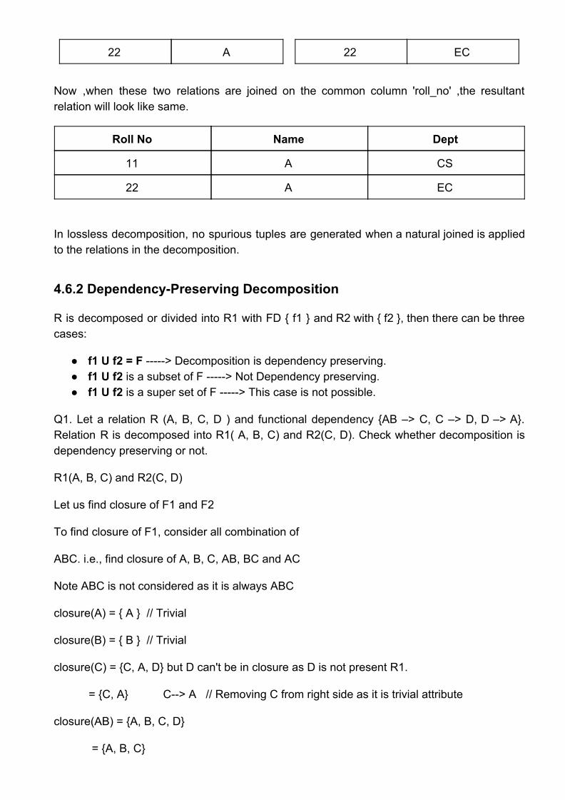
Now ,when these two relations are joined on the common column 'roll_no' ,the resultant relation will look like same.

Roll No Name Dept

11 A CS

22 A EC

In lossless decomposition, no spurious tuples are generated when a natural joined is applied to the relations in the decomposition.

4.6.2 Dependency-Preserving Decomposition

R is decomposed or divided into R1 with FD { f1 } and R2 with { f2 }, then there can be three cases:

● f1 U f2 = F -----> Decomposition is dependency preserving. ● f1 U f2 is a subset of F -----> Not Dependency preserving. ● f1 U f2 is a super set of F -----> This case is not possible.

Q1. Let a relation R (A, B, C, D ) and functional dependency {AB –> C, C –> D, D –> A}. Relation R is decomposed into R1( A, B, C) and R2(C, D). Check whether decomposition is dependency preserving or not.

R1(A, B, C) and R2(C, D)

Let us find closure of F1 and F2

To find closure of F1, consider all combination of

ABC. i.e., find closure of A, B, C, AB, BC and AC

Note ABC is not considered as it is always ABC

closure(A) = { A } // Trivial

closure(B) = { B } // Trivial

closure(C) = {C, A, D} but D can't be in closure as D is not present R1.

= {C, A} C--> A // Removing C from right side as it is trivial attribute

closure(AB) = {A, B, C, D}

= {A, B, C}

AB --> C // Removing AB from right side as these are trivial attributes

closure(BC) = {B, C, D, A}

= {A, B, C}

BC --> A // Removing BC from right side as these are trivial attributes

closure(AC) = {A, C, D}

AC --> D // Removing AC from right side as these are trivial attributes

F1 {C--> A, AB --> C, BC --> A}.

Similarly F2 { C--> D }

In the original Relation Dependency { AB --> C , C --> D , D --> A}.

AB --> C is present in F1.

C --> D is present in F2.

D --> A is not preserved.

F1 U F2 is a subset of F. So given decomposition is not dependency preservingg.