Embed Size (px)
Citation preview
CE -751, SLD, Class Notes, Fall 2006, IIT Bombay
18
Module 2
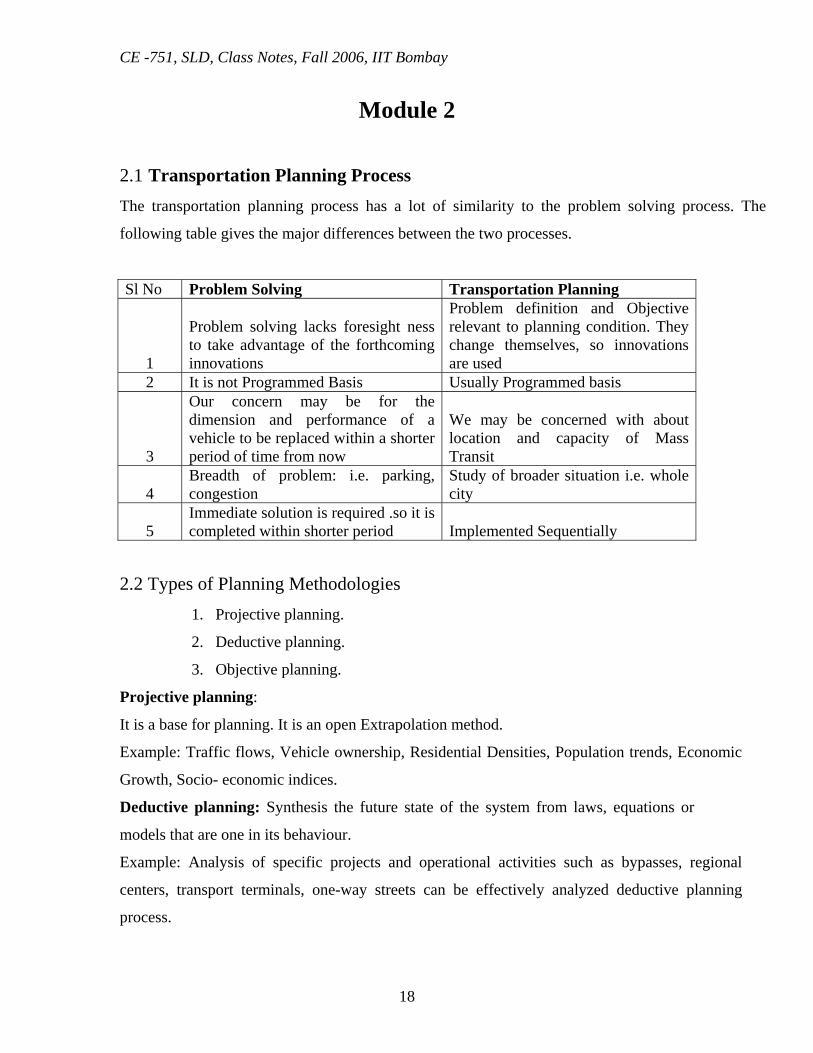
2.1 Transportation Planning Process The transportation planning process has a lot of similarity to the problem solving process. The
following table gives the major differences between the two processes.
Sl No Problem Solving Transportation Planning
1
Problem solving lacks foresight ness to take advantage of the forthcoming innovations
Problem definition and Objective relevant to planning condition. They change themselves, so innovations are used
2 It is not Programmed Basis Usually Programmed basis
3
Our concern may be for the dimension and performance of a vehicle to be replaced within a shorter period of time from now
We may be concerned with about location and capacity of Mass Transit
4 Breadth of problem: i.e. parking, congestion
Study of broader situation i.e. whole city
5 Immediate solution is required .so it is completed within shorter period Implemented Sequentially
2.2 Types of Planning Methodologies 1. Projective planning.
2. Deductive planning.
3. Objective planning.
Projective planning:
It is a base for planning. It is an open Extrapolation method.
Example: Traffic flows, Vehicle ownership, Residential Densities, Population trends, Economic
Growth, Socio- economic indices.
Deductive planning: Synthesis the future state of the system from laws, equations or
models that are one in its behaviour.
Example: Analysis of specific projects and operational activities such as bypasses, regional
centers, transport terminals, one-way streets can be effectively analyzed deductive planning
process.
CE -751, SLD, Class Notes, Fall 2006, IIT Bombay
19
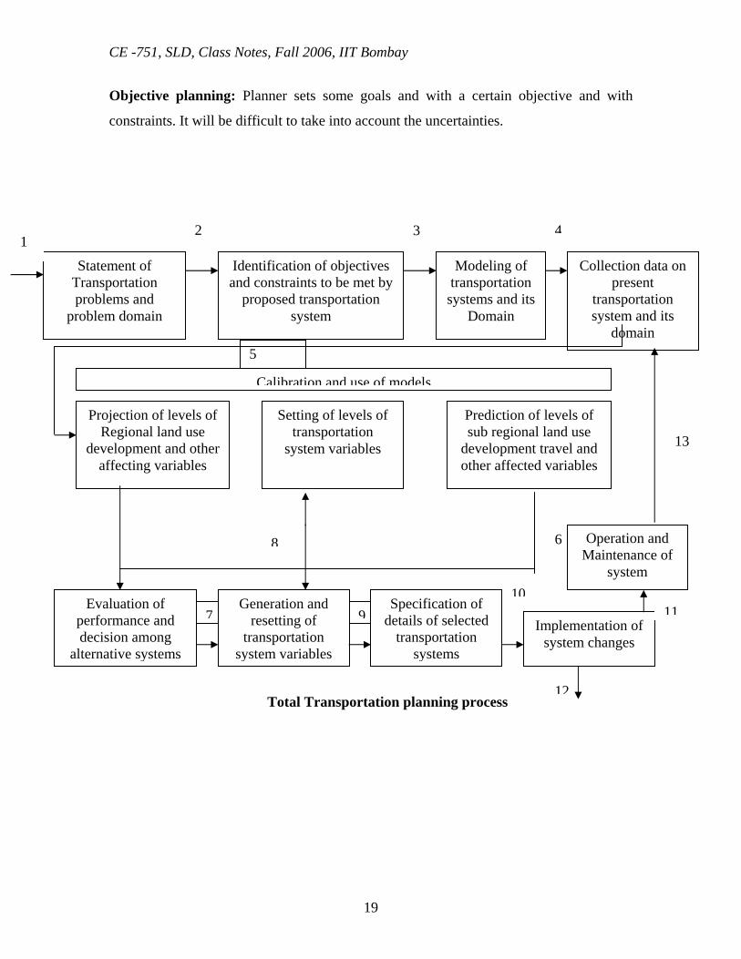
Objective planning: Planner sets some goals and with a certain objective and with
constraints. It will be difficult to take into account the uncertainties.
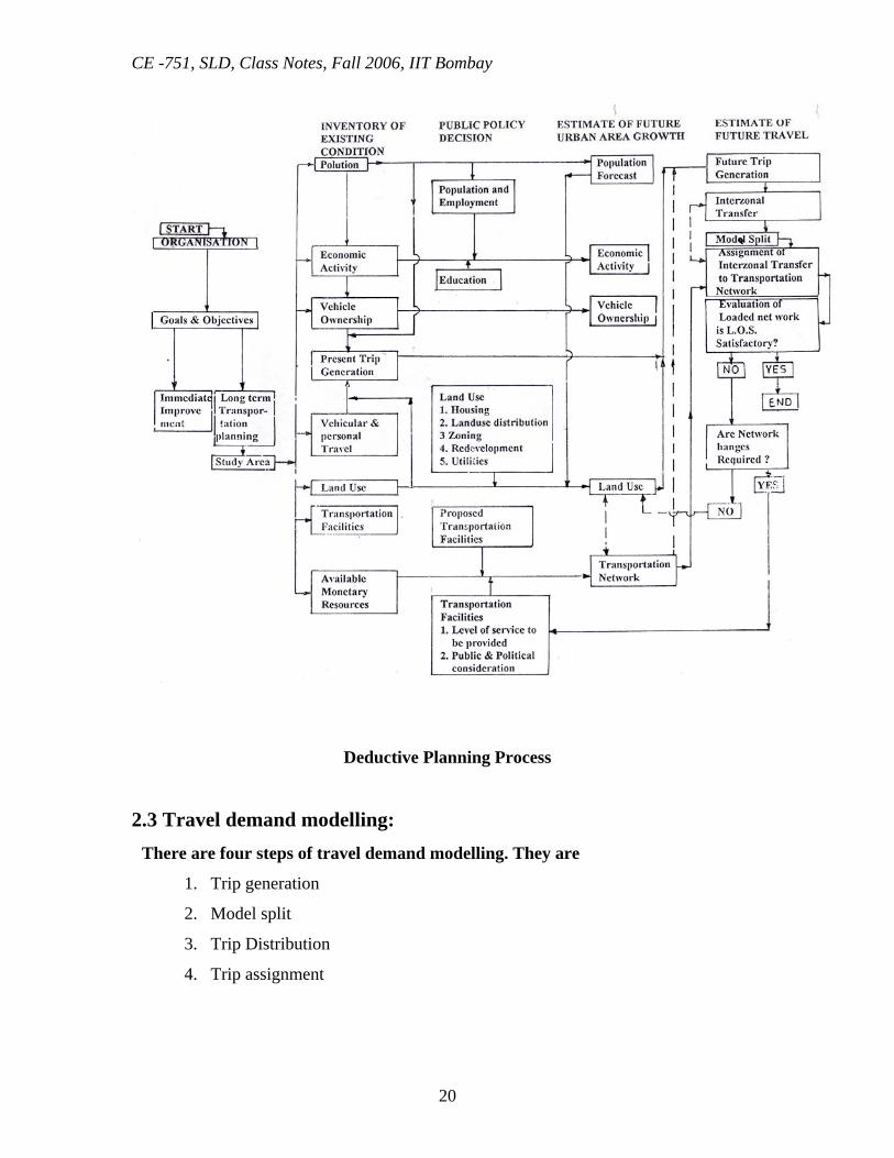
Total Transportation planning process
5
6
7 910
8
12
Statement of Transportation problems and
problem domain
Identification of objectives and constraints to be met by
proposed transportation system
Modeling of transportation systems and its
Domain
Collection data on present
transportation system and its
domain
Projection of levels of Regional land use
development and other affecting variables
Setting of levels of transportation
system variables
Prediction of levels of sub regional land use
development travel and other affected variables
Calibration and use of models
Evaluation of performance and decision among
alternative systems
Generation and resetting of
transportation system variables
Specification of details of selected
transportation systems
Implementation of system changes
Operation and Maintenance of
system
1 2 3 4
11
13
CE -751, SLD, Class Notes, Fall 2006, IIT Bombay
20
Deductive Planning Process
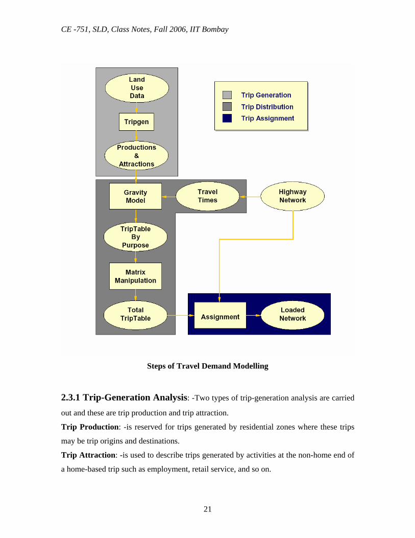
2.3 Travel demand modelling: There are four steps of travel demand modelling. They are
1. Trip generation
2. Model split
3. Trip Distribution
4. Trip assignment
CE -751, SLD, Class Notes, Fall 2006, IIT Bombay
21
Steps of Travel Demand Modelling
2.3.1 Trip-Generation Analysis: -Two types of trip-generation analysis are carried
out and these are trip production and trip attraction.
Trip Production: -is reserved for trips generated by residential zones where these trips
may be trip origins and destinations.
Trip Attraction: -is used to describe trips generated by activities at the non-home end of
a home-based trip such as employment, retail service, and so on.
CE -751, SLD, Class Notes, Fall 2006, IIT Bombay
22
The first activity in travel-demand forecasting is to identify the various trip types
important to a particular transport-planning study. The trip types studied in a particular
area depend on the types of transport-planning issues to be resolved. The first level of trip
classification used normally is a broad grouping into home-based and non-home-based
trips.
Home-based Trips: - are those trips that have one trip end at a household. Examples
journey to work, shop, school etc.
Non-home-based trips: -are trips between work and shop and business trips between two
places of employment.
Trip classification that have been used in the major transport-planning studies for
home-based trips are:
a. Work trips
b. School trips
c. Shopping trips
d. Personnel business trips, and
e. Social-recreational trips
Factors influencing Trip Production
Households may be characterized in many ways, but a large number of trip-production
studies have shown that the following variables are the most important characteristics
with respect to the major trip trips such as work and shopping trips:
1. The number of workers in a household, and
2. The household income or some proxy of income, such as the number of cars per
household.
Factors Influencing Trip Attraction
Depending on the floor areas, the trip attraction can be determined from retail floor area,
service and office floor area and manufacturing and wholesaling floor area.
Multiple Regression Analysis
The majority of trip-generation studies performed have used multiple regression analysis
to develop the prediction equations for the trips generated by various types of land use.
CE -751, SLD, Class Notes, Fall 2006, IIT Bombay
23
Most of these regression equations have been developed using a stepwise regression
analysis computer program. Stepwise regression –analysis programs allow the analyst to
develop and test a large number of potential regression equations using various
combinations and transformations of both the dependent and independent variables. The
planner may then select the most appropriate prediction equation using certain statistical
criteria. In formulating and testing various regression equations, the analyst must have a
thorough understanding of the theoretical basis of the regression analysis.
Review of Regression Analysis Concept
Some of the fundamental of regression analysis: - The principal assumptions of
regression analysis are:
1. The variance of the Y values about the regression line must be the same for all
magnitudes of the independent variables.
2. The deviations of the Y values about the regression line must be independent of
each other and normally distributed.
3. The X values are measured without error
4. The regression of the dependent variable Y on the independent variable X is
linear.
Assume that observation of the magnitude of a dependent variable Y have been obtained
for N magnitudes of an independent variable X and that on an equation of the form
bXaYe += is to be fitted to the data where eY is an estimated magnitude rather than an
observed value Y .
From the least-squares criterion, the magnitude of the parameters a and b may be
estimated.
∑∑= 2x
xyb
XbYa −=
where
XXx −= and YYy −=
CE -751, SLD, Class Notes, Fall 2006, IIT Bombay
24
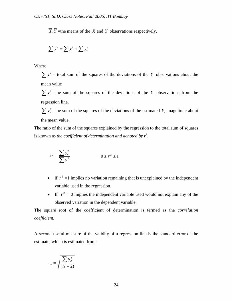
YX , =the means of the X and Y observations respectively.
∑∑∑ += 222ed yyy
Where
∑ 2y = total sum of the squares of the deviations of the Y observations about the
mean value
∑ 2dy =the sum of the squares of the deviations of the Y observations from the
regression line.
∑ 2ey =the sum of the squares of the deviations of the estimated eY magnitude about
the mean value.
The ratio of the sum of the squares explained by the regression to the total sum of squares
is known as the coefficient of determination and denoted by r2.
∑∑= 2
22
yy
r e 10 2 ≤≤ r
• if 2r =1 implies no variation remaining that is unexplained by the independent
variable used in the regression.
• If 2r = 0 implies the independent variable used would not explain any of the
observed variation in the dependent variable.
The square root of the coefficient of determination is termed as the correlation
coefficient.
A second useful measure of the validity of a regression line is the standard error of the
estimate, which is estimated from:
)2(
2
−= ∑
Ny
s de
CE -751, SLD, Class Notes, Fall 2006, IIT Bombay
25
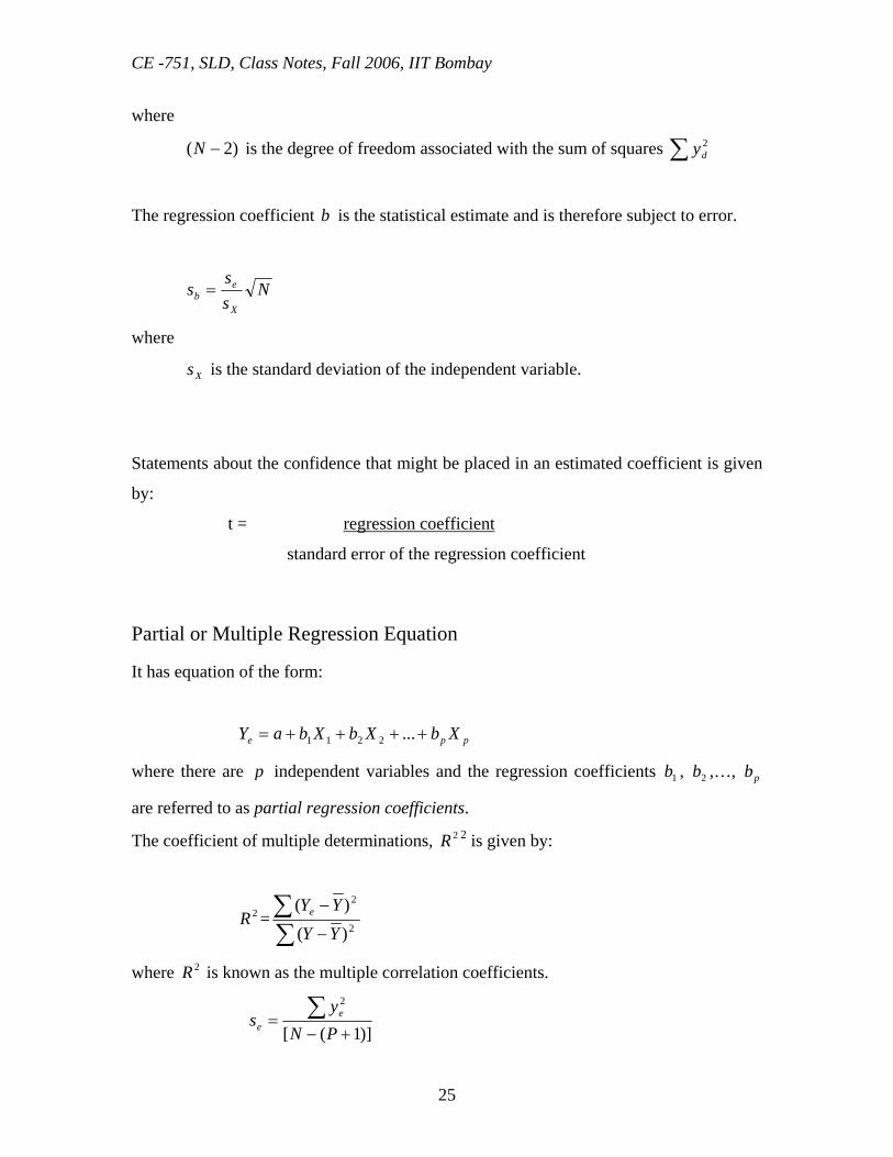
where
)2( −N is the degree of freedom associated with the sum of squares ∑ 2dy
The regression coefficient b is the statistical estimate and is therefore subject to error.
Nss
sX
eb =
where
Xs is the standard deviation of the independent variable.
Statements about the confidence that might be placed in an estimated coefficient is given
by:
t = regression coefficient
standard error of the regression coefficient
Partial or Multiple Regression Equation
It has equation of the form:
ppe XbXbXbaY ++++= ...2211
where there are p independent variables and the regression coefficients 1b , 2b ,…, pb
are referred to as partial regression coefficients.
The coefficient of multiple determinations, 2R 2 is given by:
2R =∑∑
−
−2
2
)()(
YYYYe
where 2R is known as the multiple correlation coefficients.
)]1([
2
+−= ∑
PNy
s ee
CE -751, SLD, Class Notes, Fall 2006, IIT Bombay
26
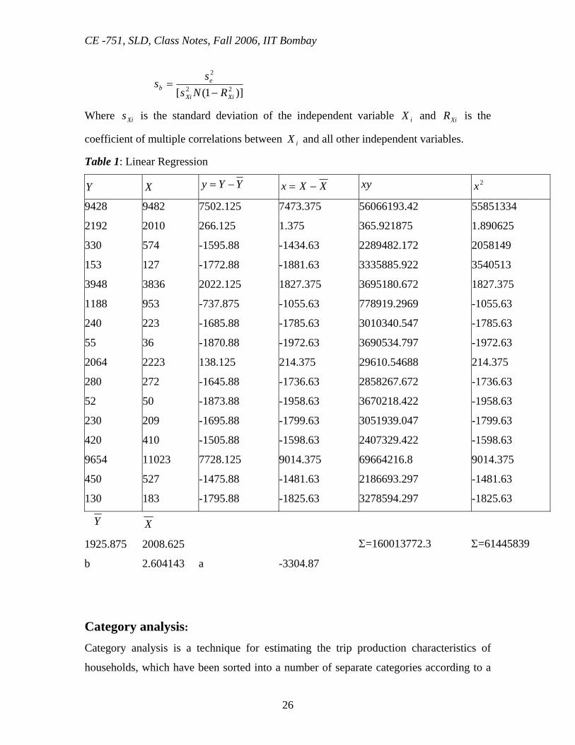
)]1([ 22
2
XiXi
eb RNs
ss
−=
Where Xis is the standard deviation of the independent variable iX and XiR is the
coefficient of multiple correlations between iX and all other independent variables.
Table 1: Linear Regression
Y X YYy −= XXx −= xy 2x
9428 9482 7502.125 7473.375 56066193.42 55851334
2192 2010 266.125 1.375 365.921875 1.890625
330 574 -1595.88 -1434.63 2289482.172 2058149
153 127 -1772.88 -1881.63 3335885.922 3540513
3948 3836 2022.125 1827.375 3695180.672 1827.375
1188 953 -737.875 -1055.63 778919.2969 -1055.63
240 223 -1685.88 -1785.63 3010340.547 -1785.63
55 36 -1870.88 -1972.63 3690534.797 -1972.63
2064 2223 138.125 214.375 29610.54688 214.375
280 272 -1645.88 -1736.63 2858267.672 -1736.63
52 50 -1873.88 -1958.63 3670218.422 -1958.63
230 209 -1695.88 -1799.63 3051939.047 -1799.63
420 410 -1505.88 -1598.63 2407329.422 -1598.63
9654 11023 7728.125 9014.375 69664216.8 9014.375
450 527 -1475.88 -1481.63 2186693.297 -1481.63
130 183 -1795.88 -1825.63 3278594.297 -1825.63
Y X
1925.875 2008.625 Σ=160013772.3 Σ=61445839
b 2.604143 a -3304.87
Category analysis:
Category analysis is a technique for estimating the trip production characteristics of
households, which have been sorted into a number of separate categories according to a
CE -751, SLD, Class Notes, Fall 2006, IIT Bombay
27
set of properties that characterize the household. Category analysis may also be used to
estimate trip attractions.
Zonal trip productions may be estimated as
)()( ctpchp iqi ∑=
Where,
qip = The number of trips produced by zone i by type q people.
hi(c)= number of households in zone i in category c
tp( c)= trip production rate of a household category c.
Zonal trip-attractions may be estimated as
)()( ctacba jj ∑=
Where,
aj = number of work trips attracted by zone j.
bj(c) = number of employment opportunities in category c.
ta(c) = trip attraction rate of employment category c
And the summation is over all employment types if work trip attractions are to be
estimated.
2.3.2 Modal Split The second stage of travel demand forecasting process has bee identified as captive
modal split analysis. The second stage of modal split analysis was identified as occurring
after the trip distribution analysis phase. Two submarkets for public transportation
services have been labelled as captive transit riders and choice transit riders. The aim of
captive modal split analysis is to establish relationships that allow the trip ends estimated
in the trip generation phase to be partitioned into captive transit riders and choice transit
riders. The purpose of choice modal split analysis phase is to estimate the probable split
CE -751, SLD, Class Notes, Fall 2006, IIT Bombay
28
of choice transit riders between public transport and car travel given measures of
generalized cost of travel by two modes.
The ratio of choice trip makers using a public transport system varies from 9 to 1 in
small cities with poorly developed public transport systems to as high as 3 to 1 in well
developed cities.
Major determinants of Public Patronage are
1. Socio economic characteristics of trip makers
2. Relative cost and service properties of the trip by car and that by public transport.
Variables used to identify the status at the household level are
1. Household income or car ownership directly
2. The number of persons per household.
3. The age and sex of household members.
4. The purpose of the trip.
The modal split models, which have been used before the trip distribution phase, are
usually referred to as trip end modal split models. Modal split that have followed the trip
distribution phase are normally termed trip interchange modal spit models. Trip end
modal split models are used today in medium and small sized cities. The basic
assumption of the trip end type models is that transport patronage is relatively insensitive
to the service characteristics to the transport modes. Modal patronages are determined
principally by the socio economic characteristics of the trip makers. Most of the trip
interchanges modal split models incorporate measures of relative service characteristics
of competing modes as well as measures of the socio economic characteristics of the trip
makers. The modal split model developed during the southeastern Wisconsin
transportation study is an example of trip end type model. The model-split model
developed in Toronto is an example of trip interchange modal split model.
Land Use
CE -751, SLD, Class Notes, Fall 2006, IIT Bombay
29
These factors, including time and cost, can be grouped into three broad categories.
• Characteristics of the traveler -- the trip maker;
• Characteristics of the trip; and
• Characteristics of the transportation system.
Southeastern Wisconsin Model: This Model consisted of seven estimating surfaces that related the percentage of the trip
ends that will use transit services from a particular traffic analysis zone to the following
variables: trip type, characteristics of trip maker and characteristics of the transport
system. The trips made by public transport services are classified as Home based work
trips, home based shopping trips, home based other trips and non-home based trips. The
Trip Generation equation
Modal split model Trip Distribution models
Trip ends by mode Origin-Destination Volumes
Trip Distribution model Modal split model
O-D Volumes by mode O-D Volumes by mode
Trip End Type Modal Split Model Trip Interchange Type Modal Split Model
CE -751, SLD, Class Notes, Fall 2006, IIT Bombay
30
socioeconomic characteristics of trip makers were defined on the zonal basis in terms of
average number of cars per household in a zone. The characteristics of a transport system
relative to given zone were defined by an accessibility index which is given by:
ij
n
jji faacc ∑
=
=1
Where
iacc = accessibility index for zone i
ja = No of attractions in zone j
ijf = Travel time factor for travel from zone I to zone j for a particular mode being
considered.
The transport service provided to a particular zone by two modes was characterized by
accessibility ratio.
Accessibility Ratio = Highway accessibility index / Transit accessibility index.
Toronto Model: Trip interchange modal split models allocate trips between public transport and private
transport after trip distribution stage. The split between two modes is assumed to be a
function of the following transportation variables between each pair of zones, as well as
the socioeconomic characteristics of the people who avail themselves of the alternatives
Relative Travel Time (TTR)
Relative Travel Cost
Economic status of the Trip maker
Relative travel service
876
54321
XXXXXXXX
TTR++
++++=

CE -751, SLD, Class Notes, Fall 2006, IIT Bombay
31
Where
X1 = Time spent in transit vehicle
X2 =Transfer time between transit vehicles
X3 = Time spent in waiting for a transit vehicle
X4 = Walking time to a transit vehicle
X5 = Walking time for transit vehicle
X6 = Auto driving time
X7 = Parking delay at destination
X8 = Walking time from parking place to destination
This represents the door to door travel time to train to that of automobiles
13
121110
9
X)X5.0X(X
X++
=CR
Where
X9 =Transit Fare
X10 =Cost of gasoline
X11 =Cost of oil charge and lubrication
X12 =Parking Cost at destination
X13 = Average Car Occupancy
The denominator indicates that auto cost must be put on a person per one way trip basis
in order to be comparable to the costs for transit.
The variable EC is defined in terms of medium income per worker in the zone of trip
production. The variable D is designed arbitrarily as
87
5432
XXXXXX
D+
+++=
MODAL SPLIT MODEL WITH A BEHAVIOURAL ANALYSIS

CE -751, SLD, Class Notes, Fall 2006, IIT Bombay
32
The focus of these models is on individual behavior rather than on zonally aggregated
modal choice behaviour. Central to these methods is the concept of trip disutility or the
generalized cost of using different modes of transport.
Generalized cost of travel:
The concept of generalized travel cost is derived from the notion that the trip making has
a number of characteristics which are unpleasant to trip makers and that the magnitudes
of this unpleasantness depend on the socioeconomic characteristics of the trip maker. The
generalized cost or disutility of a trip may be estimated from:
cubxaz wwmnijn
mij ++=
n=1,…………….n,
w=1,…………….w.
Where,
mijz = generalized cost of travel between zones I and j by mode m.
mnijx = the nth characteristic of mode m between zones I and j which gives rise to the cost
of travel by mode m.
wu = the wth socioeconomic characteristic of a tripmaker.
c = constant.
na , wb = coefficients that reflect the relative contribution that system and tripmaker
characteristics make to the generalized cost of travel.
For a binary modal choice situation the following generalized cost difference may be
calculated from the above equation.
cubxaz wwnijnij ++Δ=*
n=1,……………….n,
w=1,……………….w.
where, *ijz = the difference in generalized costs of travelling between zones i and j.
nijxΔ = the difference in the nth system characteristic between the two modes.
CE -751, SLD, Class Notes, Fall 2006, IIT Bombay
33
If trip makers are classified into a number of socioeconomic groups, then may be
expressed as
cxaz nijnij +Δ=*
n=1,……………,n
if *ijz is the difference in cost between transit and car travel then c may be regarded as a
mode penalty reflecting the inferior convenience and comfort of transit relative to car.
Wilson and his associates reported the following generalized cost relationship from
studies in England. mij
mij
mij
mij saedz 332.166.0 ++=
Where
mijz = The generalized cost of travelling between zones i and j by modes m
mijd = The in vehicle travel time in minutes by mode m between zones i and j.
mije = The excess travel time in minutes by mode m between zones i and j.
mijs = The distance in miles by mode m between zones i and j.
a3 = 2.0 for car travel
2.18 for train travel
3.06 for bus travel.
BINARY CHOICE STOCHASTIC MODAL SPLIT MODELS:
This is one of the models which deal with the generalized costs of travel for competing
modes. Three types of mathematical concepts have been used to construct stochastic
modal choice functions for the individual behaviour:
• Discriminant analysis
• Probit analysis
• Logit analysis.
CE -751, SLD, Class Notes, Fall 2006, IIT Bombay
34
Discriminant analysis
The basic premise is that the choice of tripmakers in an urban area may be classified into
two groups according to mode of transport used. The objective is to find a linear
combination of explanatory variables that possesses little overlap. The best discriminate
function is the one that minimizes the number of mis classifications of trip makers to the
observed transport modes.
Quarmby, has developed an equation for estimating car bus modal split for work trips to
central London:
)431.0(04.1
)431.0(04.1
26.2126.2)/( −
−
+= z
z
eezcpr
pr(c/z)= the probability of choosing the car mode- given that the travel disutility is z.
The disutility measure was developed as a function of differences in total travel time,
excess travel time, costs and income related variables.
Talvitie model:
)/ln(
)/ln(
1)/1( yxz
yxz
eeijmpr +
+
+==
)/ln(11)/2( yxze
ijmpr ++==
z is assumed to be normally distributed.
Where
Pr(m/ij) = the probability that an individual will use mode m given that the trip is
between zones i and j.
x, y = The a priori probabilities of membership in groups m=1 and m=2 respectively.
Probit Analysis
The basic premise is that as choice trip makers are subjected to changing magnitudes of
relative trip costs, the proportion of trip makers that respond by choosing a particular
mode of transport will follow a linear relation.
Lave has developed the following equation for estimating the probability of bus-car
modal patronage for Chicago area.
AIDCcTkWY c 0255.00254.00186.000759.008.2 +−Δ+Δ+−=
R2 = 0.379
CE -751, SLD, Class Notes, Fall 2006, IIT Bombay
35
Where
Y= binary variable with positive magnitudes denoting transit riders and negative
magnitudes denoting car riders.
TkWΔ = time difference between modes multiplied by the tripmaker’s wage rate
and his marginal preference for leisure time.
cIDC = a binary valued comfort variable multiplied by income and trip distance.
Logit Analysis:
Stopher model.
*
*
1)/1(
ij
ij
z
z
e
eijmpr+
==
*
1
1)/2(ijze
ijmpr+
==
where
zij* = some function of the generalized costs of travel by modes m=1 and m=2
Two Stage Modal Split Model Vandertol et al. have developed a simple two stage model which recognizes explicitly the
existence of both captive and of choice transit riders. The model first identifies both the
production and attraction trip ends of transit captives and choice transit riders separately.
The two groups of trip makers are then distributed from origin to destinations. The choice
transit riders are then split between transit and car according to a choice modal split
model, which reflects the relative characteristics of the trip by transit and the trip by car.
In most cities, the transit captive is severely restricted in the choice of both household and
employment locations. Studies in a number of cities have shown that the trip ends of the
transit captives tend to be clustered in zones that are well served by public transport. The
challenge is to develop is to formulate a technique that uses information normally
available in urban areas.
Zonal work trip productions disaggregated by the captive and the choice transit riders
may be estimated from
Pi q = hitpq
CE -751, SLD, Class Notes, Fall 2006, IIT Bombay
36
Where
Pi q = no of work trips produced in zone i by type q trip makers
hi = the no of households in zone i
tpq = work trip production rate for trip maker group q which is a function of
economic status of a zone and the average no of employees per household.
The work trips attracted to each zone j by trip maker type q may be estimated from
ajq= [prc
q] [rct] [etj]
Where
ajq= the no of work trips of type q trip maker attracted to zone j
[prcq] = A row vector of the probability of the trip maker type q being in occupation
category type c.
[rct] = A c*t matrix of the probabilities of an occupation category type c within an
industry type t.
[etj] = a t*j matrix of the no of jobs within each industry type t in each zone j.
2.4 TRIP DISTRIBUTION A trip distribution model produces a new origin-destination trip matrix to reflect new
trips in the future made by population, employment and other demographic changes so as
to reflect changes in people's choice of destination. They are used to forecast the origin-
destination pattern of travel into the future and produce a trip matrix, which can be
assigned in an assignment model of put into a mode choice model. The trip matrix can
change as a result of improvements in the transport system or as a result of new
developments, shops, offices etc and the distribution model seeks to model these effects
so as to produce a new trip matrix for the future travel situation.
Trip distribution models connect the trip origins and destination estimated by the trip
generation models to create estimated trips. Different trip distribution models are
developed for each of the trip purposes for which trip generation has been
estimated.Various techniques developed for trip distribution modeling are
• Growth Factor Models
• Synthetic Models
CE -751, SLD, Class Notes, Fall 2006, IIT Bombay
37
Growth Factor Models
• Uniform Factor Method
• Average Factor Method
• Detroit Method
• Fratar Method
• Furness Method
• Furness Time-function Iteration
Synthetic Models
• Gravity/Spatial Interaction Models
• Opportunity Models
• Regression/Econometric Models
• Optimization Models
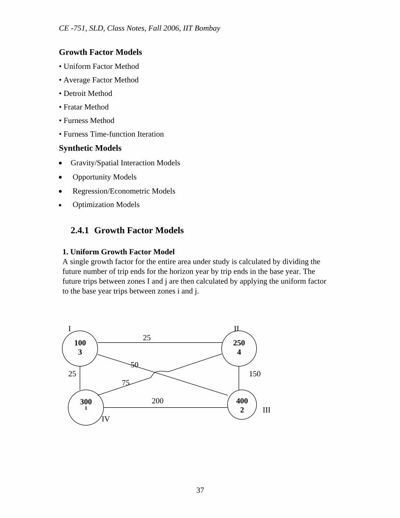
2.4.1 Growth Factor Models 1. Uniform Growth Factor Model A single growth factor for the entire area under study is calculated by dividing the future number of trip ends for the horizon year by trip ends in the base year. The future trips between zones I and j are then calculated by applying the uniform factor to the base year trips between zones i and j. I II 25 50 25 150 75 200 III IV
100 3
300 1
400 2
250 4
CE -751, SLD, Class Notes, Fall 2006, IIT Bombay
38
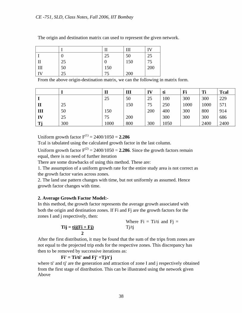
The origin and destination matrix can used to represent the given network. I II III IV I 0 25 50 25 II 25 0 150 75 III 50 150 200 IV 25 75 200 From the above origin-destination matrix, we can the following in matrix form. I II III IV ti Fi Ti Tcal I 25 50 25 100 300 300 229 II 25 150 75 250 1000 1000 571 III 50 150 200 400 300 800 914 IV 25 75 200 300 300 300 686 Tj 300 1000 800 300 1050 2400 2400 Uniform growth factor F(1) = 2400/1050 = 2.286 Tcal is tabulated using the calculated growth factor in the last column. Uniform growth factor F(2) = 2400/1050 = 2.286. Since the growth factors remain equal, there is no need of further iteration There are some drawbacks of using this method. These are: 1. The assumption of a uniform growth rate for the entire study area is not correct as the growth factor varies across zones. 2. The land use pattern changes with time, but not uniformly as assumed. Hence growth factor changes with time. 2. Average Growth Factor Model:- In this method, the growth factor represents the average growth associated with both the origin and destination zones. If Fi and Fj are the growth factors for the zones I and j respectively, then:
Tij = tij(Fi + Fj) Where Fi = Ti/ti and Fj = Tj/tj
2 After the first distribution, it may be found that the sum of the trips from zones are not equal to the projected trip ends for the respective zones. This discrepancy has then to be removed by successive iterations as: Fi' = Ti/ti' and Fj' =Tj/t'j where ti' and tj' are the generation and attraction of zone I and j respectively obtained from the first stage of distribution. This can be illustrated using the network given Above
CE -751, SLD, Class Notes, Fall 2006, IIT Bombay
39
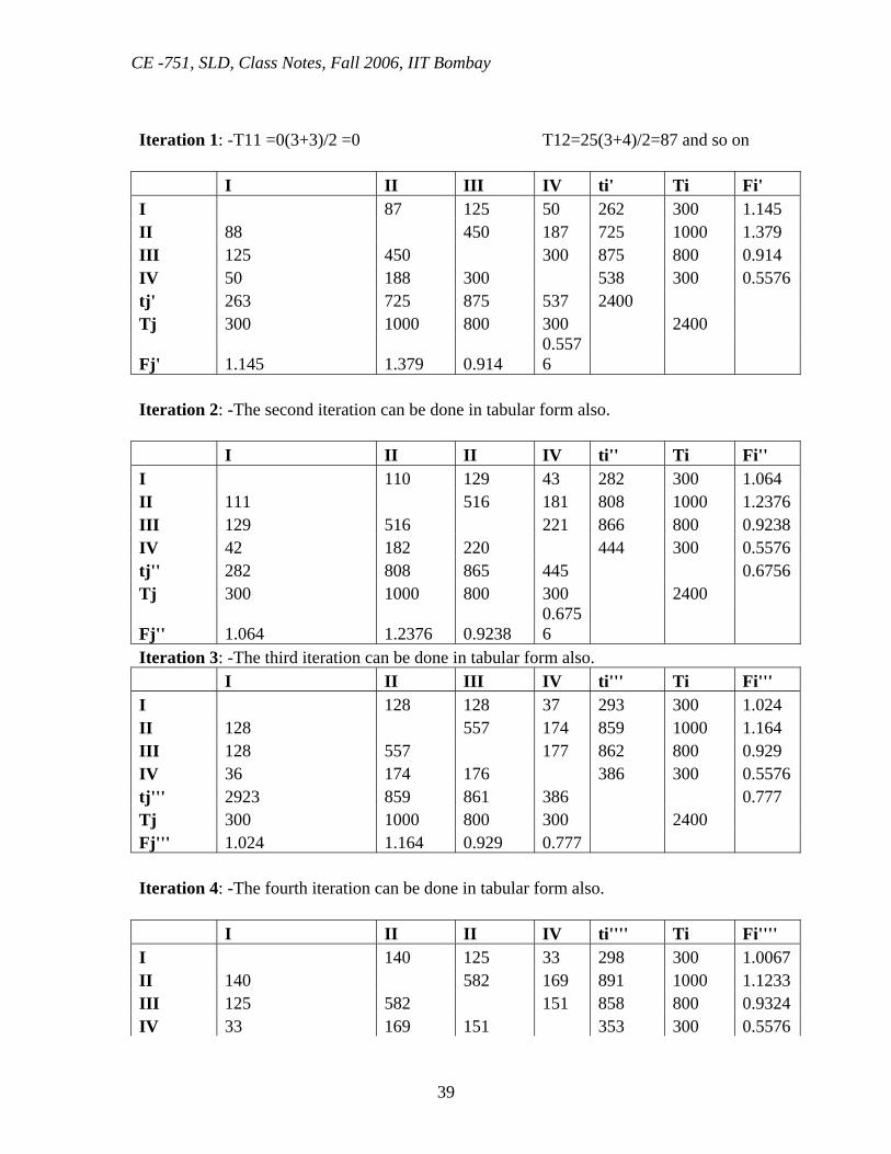
Iteration 1: -T11 =0(3+3)/2 =0 T12=25(3+4)/2=87 and so on I II III IV ti' Ti Fi' I 87 125 50 262 300 1.145 II 88 450 187 725 1000 1.379 III 125 450 300 875 800 0.914 IV 50 188 300 538 300 0.5576 tj' 263 725 875 537 2400 Tj 300 1000 800 300 2400
Fj' 1.145 1.379 0.914 0.5576
Iteration 2: -The second iteration can be done in tabular form also. I II II IV ti'' Ti Fi'' I 110 129 43 282 300 1.064 II 111 516 181 808 1000 1.2376 III 129 516 221 866 800 0.9238 IV 42 182 220 444 300 0.5576 tj'' 282 808 865 445 0.6756 Tj 300 1000 800 300 2400
Fj'' 1.064 1.2376 0.9238 0.6756
Iteration 3: -The third iteration can be done in tabular form also. I II III IV ti''' Ti Fi''' I 128 128 37 293 300 1.024 II 128 557 174 859 1000 1.164 III 128 557 177 862 800 0.929 IV 36 174 176 386 300 0.5576 tj''' 2923 859 861 386 0.777 Tj 300 1000 800 300 2400 Fj''' 1.024 1.164 0.929 0.777 Iteration 4: -The fourth iteration can be done in tabular form also. I II II IV ti'''' Ti Fi'''' I 140 125 33 298 300 1.0067 II 140 582 169 891 1000 1.1233 III 125 582 151 858 800 0.9324 IV 33 169 151 353 300 0.5576
CE -751, SLD, Class Notes, Fall 2006, IIT Bombay
40
tj'''' 298 891 858 353 0.8498 Tj 300 1000 800 300 2400
Fj'''' 1.0067 1.1233 0.9324 0.8498
Iteration 5: -The fifth iteration can be done in tabular form also. I II II IV ti''''' Ti Fi''''' I 149 121 31 301 300 0.99 II 149 599 166 914 1000 1.09
III 121 599 134 854 800 0.93677
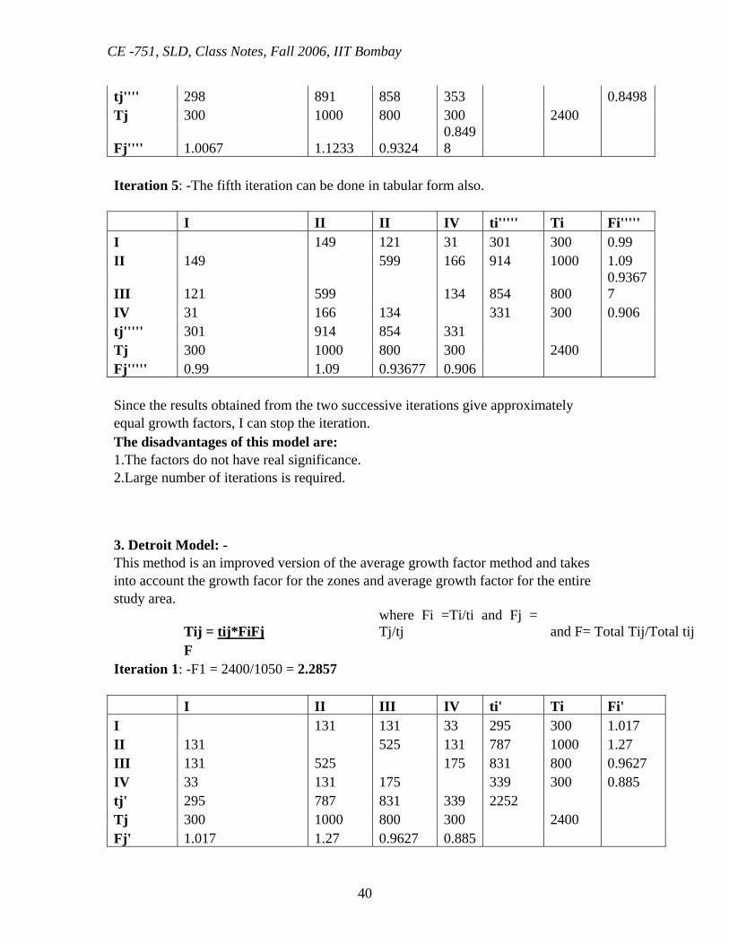
IV 31 166 134 331 300 0.906 tj''''' 301 914 854 331 Tj 300 1000 800 300 2400 Fj''''' 0.99 1.09 0.93677 0.906 Since the results obtained from the two successive iterations give approximately equal growth factors, I can stop the iteration. The disadvantages of this model are: 1.The factors do not have real significance. 2.Large number of iterations is required. 3. Detroit Model: - This method is an improved version of the average growth factor method and takes into account the growth facor for the zones and average growth factor for the entire study area.
Tij = tij*FiFj where Fi =Ti/ti and Fj = Tj/tj and F= Total Tij/Total tij
F Iteration 1: -F1 = 2400/1050 = 2.2857 I II III IV ti' Ti Fi' I 131 131 33 295 300 1.017 II 131 525 131 787 1000 1.27 III 131 525 175 831 800 0.9627 IV 33 131 175 339 300 0.885 tj' 295 787 831 339 2252 Tj 300 1000 800 300 2400 Fj' 1.017 1.27 0.9627 0.885
CE -751, SLD, Class Notes, Fall 2006, IIT Bombay
41
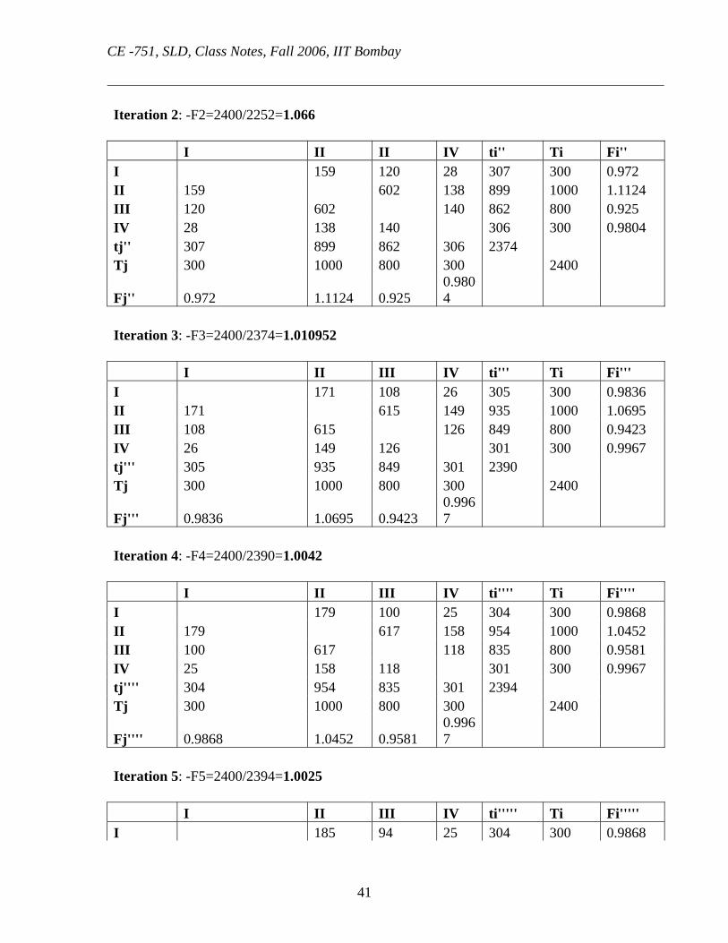
Iteration 2: -F2=2400/2252=1.066 I II II IV ti'' Ti Fi'' I 159 120 28 307 300 0.972 II 159 602 138 899 1000 1.1124 III 120 602 140 862 800 0.925 IV 28 138 140 306 300 0.9804 tj'' 307 899 862 306 2374 Tj 300 1000 800 300 2400
Fj'' 0.972 1.1124 0.925 0.9804
Iteration 3: -F3=2400/2374=1.010952 I II III IV ti''' Ti Fi''' I 171 108 26 305 300 0.9836 II 171 615 149 935 1000 1.0695 III 108 615 126 849 800 0.9423 IV 26 149 126 301 300 0.9967 tj''' 305 935 849 301 2390 Tj 300 1000 800 300 2400
Fj''' 0.9836 1.0695 0.9423 0.9967
Iteration 4: -F4=2400/2390=1.0042 I II III IV ti'''' Ti Fi'''' I 179 100 25 304 300 0.9868 II 179 617 158 954 1000 1.0452 III 100 617 118 835 800 0.9581 IV 25 158 118 301 300 0.9967 tj'''' 304 954 835 301 2394 Tj 300 1000 800 300 2400
Fj'''' 0.9868 1.0452 0.9581 0.9967
Iteration 5: -F5=2400/2394=1.0025 I II III IV ti''''' Ti Fi''''' I 185 94 25 304 300 0.9868
CE -751, SLD, Class Notes, Fall 2006, IIT Bombay
42
II 185 618 165 968 1000 1.03305 III 94 618 112 824 800 0.9709 IV 24 165 112 302 300 0.9934 tj''''' 304 968 824 302 2398 Tj 300 1000 800 300 2400
Fj''''' 0.9868 1.03305 0.9709 0.9934
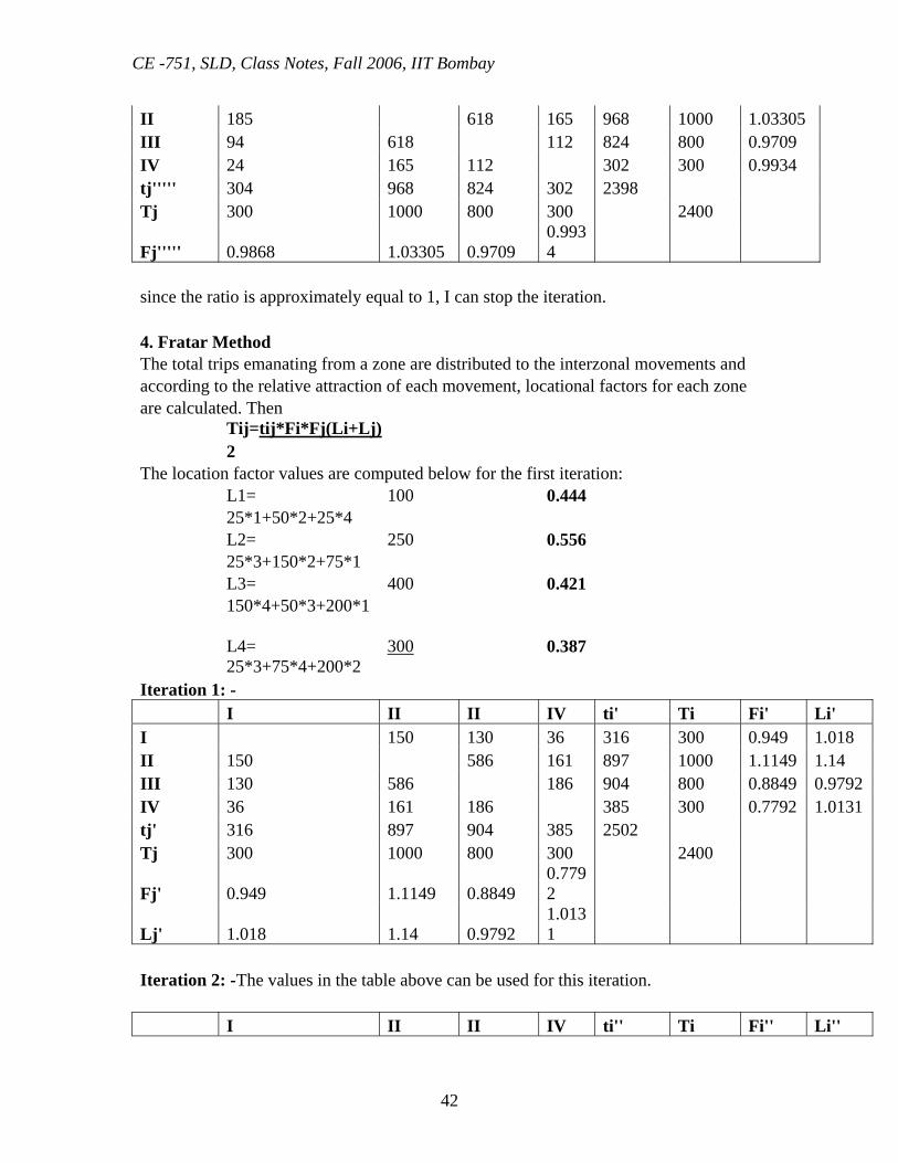
since the ratio is approximately equal to 1, I can stop the iteration. 4. Fratar Method The total trips emanating from a zone are distributed to the interzonal movements and according to the relative attraction of each movement, locational factors for each zone are calculated. Then Tij=tij*Fi*Fj(Li+Lj) 2 The location factor values are computed below for the first iteration: L1= 100 0.444 25*1+50*2+25*4 L2= 250 0.556 25*3+150*2+75*1 L3= 400 0.421 150*4+50*3+200*1
L4= 300 0.387
25*3+75*4+200*2 Iteration 1: - I II II IV ti' Ti Fi' Li' I 150 130 36 316 300 0.949 1.018 II 150 586 161 897 1000 1.1149 1.14 III 130 586 186 904 800 0.8849 0.9792 IV 36 161 186 385 300 0.7792 1.0131 tj' 316 897 904 385 2502 Tj 300 1000 800 300 2400
Fj' 0.949 1.1149 0.8849 0.7792
Lj' 1.018 1.14 0.9792 1.0131
Iteration 2: -The values in the table above can be used for this iteration. I II II IV ti'' Ti Fi'' Li''
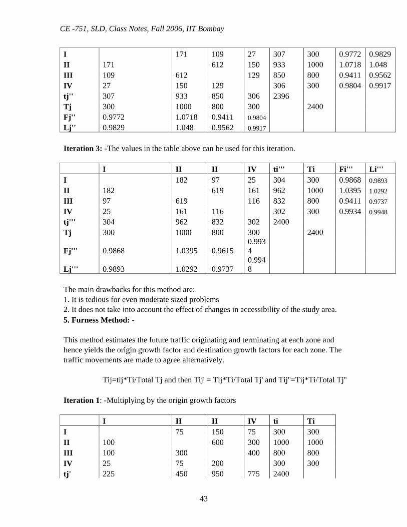
CE -751, SLD, Class Notes, Fall 2006, IIT Bombay
43
I 171 109 27 307 300 0.9772 0.9829 II 171 612 150 933 1000 1.0718 1.048 III 109 612 129 850 800 0.9411 0.9562 IV 27 150 129 306 300 0.9804 0.9917 tj'' 307 933 850 306 2396 Tj 300 1000 800 300 2400 Fj'' 0.9772 1.0718 0.9411 0.9804 Lj'' 0.9829 1.048 0.9562 0.9917 Iteration 3: -The values in the table above can be used for this iteration. I II II IV ti''' Ti Fi''' Li''' I 182 97 25 304 300 0.9868 0.9893 II 182 619 161 962 1000 1.0395 1.0292 III 97 619 116 832 800 0.9411 0.9737 IV 25 161 116 302 300 0.9934 0.9948 tj''' 304 962 832 302 2400 Tj 300 1000 800 300 2400
Fj''' 0.9868 1.0395 0.9615 0.9934
Lj''' 0.9893 1.0292 0.9737 0.9948
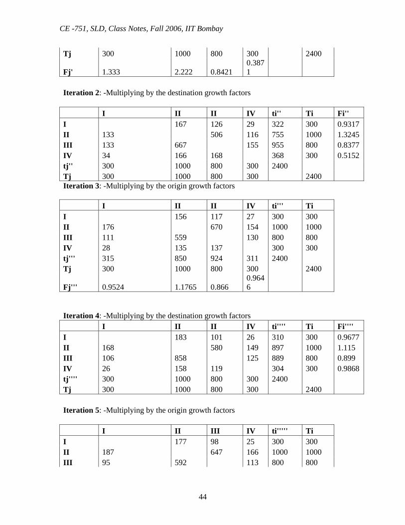
The main drawbacks for this method are: 1. It is tedious for even moderate sized problems 2. It does not take into account the effect of changes in accessibility of the study area. 5. Furness Method: - This method estimates the future traffic originating and terminating at each zone and hence yields the origin growth factor and destination growth factors for each zone. The traffic movements are made to agree alternatively. Tij=tij*Ti/Total Tj and then Tij' = Tij*Ti/Total Tj' and Tij''=Tij*Ti/Total Tj'' Iteration 1: -Multiplying by the origin growth factors I II II IV ti Ti I 75 150 75 300 300 II 100 600 300 1000 1000 III 100 300 400 800 800 IV 25 75 200 300 300 tj' 225 450 950 775 2400
CE -751, SLD, Class Notes, Fall 2006, IIT Bombay
44
Tj 300 1000 800 300 2400
Fj' 1.333 2.222 0.8421 0.3871
Iteration 2: -Multiplying by the destination growth factors I II II IV ti'' Ti Fi'' I 167 126 29 322 300 0.9317 II 133 506 116 755 1000 1.3245 III 133 667 155 955 800 0.8377 IV 34 166 168 368 300 0.5152 tj'' 300 1000 800 300 2400 Tj 300 1000 800 300 2400 Iteration 3: -Multiplying by the origin growth factors I II II IV ti''' Ti I 156 117 27 300 300 II 176 670 154 1000 1000 III 111 559 130 800 800 IV 28 135 137 300 300 tj''' 315 850 924 311 2400 Tj 300 1000 800 300 2400
Fj''' 0.9524 1.1765 0.866 0.9646
Iteration 4: -Multiplying by the destination growth factors I II II IV ti'''' Ti Fi'''' I 183 101 26 310 300 0.9677 II 168 580 149 897 1000 1.115 III 106 858 125 889 800 0.899 IV 26 158 119 304 300 0.9868 tj'''' 300 1000 800 300 2400 Tj 300 1000 800 300 2400 Iteration 5: -Multiplying by the origin growth factors I II III IV ti''''' Ti I 177 98 25 300 300 II 187 647 166 1000 1000 III 95 592 113 800 800
CE -751, SLD, Class Notes, Fall 2006, IIT Bombay
45
IV 26 157 117 300 300 tj''''' 308 926 862 304 2400 Tj 300 1000 800 300 2400
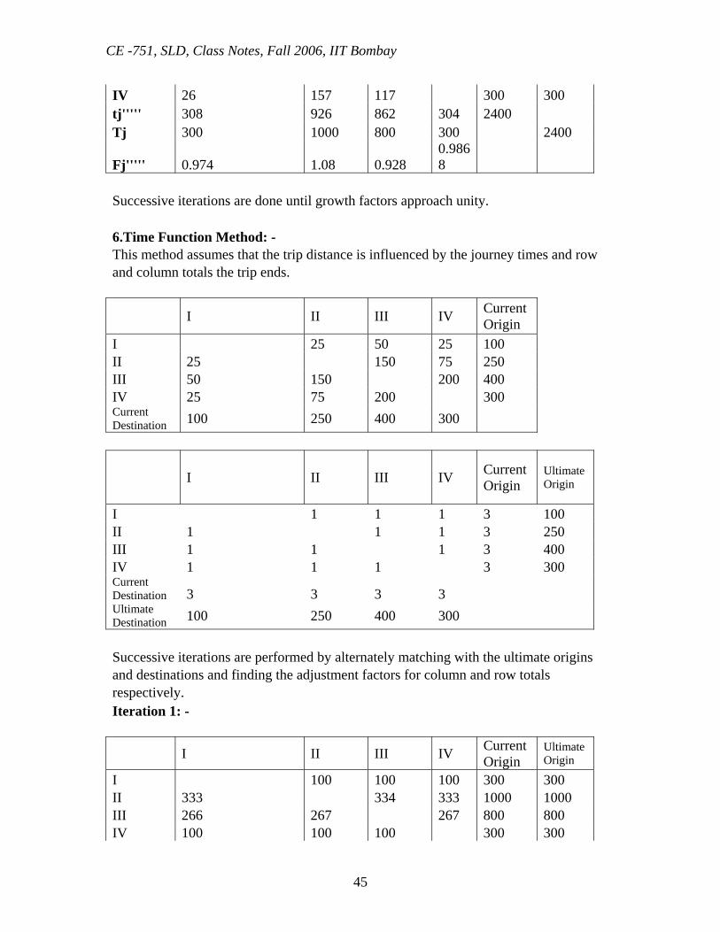
Fj''''' 0.974 1.08 0.928 0.9868
Successive iterations are done until growth factors approach unity. 6.Time Function Method: - This method assumes that the trip distance is influenced by the journey times and row and column totals the trip ends.
I II III IV Current Origin
I 25 50 25 100 II 25 150 75 250 III 50 150 200 400 IV 25 75 200 300 Current Destination 100 250 400 300
I II III IV Current Origin
UltimateOrigin
I 1 1 1 3 100 II 1 1 1 3 250 III 1 1 1 3 400 IV 1 1 1 3 300 Current Destination 3 3 3 3 Ultimate Destination 100 250 400 300 Successive iterations are performed by alternately matching with the ultimate origins and destinations and finding the adjustment factors for column and row totals respectively. Iteration 1: -
I II III IV Current Origin
UltimateOrigin
I 100 100 100 300 300 II 333 334 333 1000 1000 III 266 267 267 800 800 IV 100 100 100 300 300
CE -751, SLD, Class Notes, Fall 2006, IIT Bombay
46
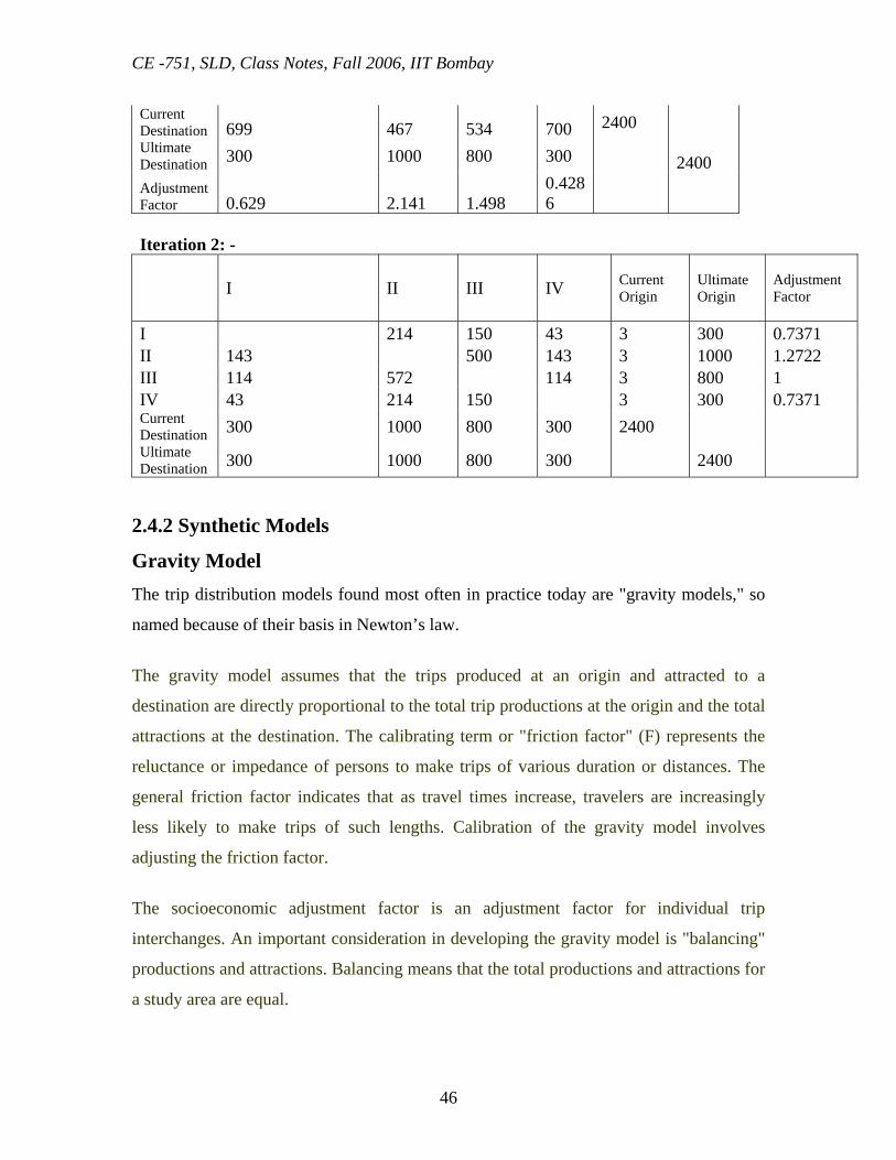
Current Destination 699 467 534 700 2400 Ultimate Destination 300 1000 800 300 2400 Adjustment Factor 0.629 2.141 1.498
0.4286
Iteration 2: -
I II III IV Current Origin
Ultimate Origin
Adjustment Factor
I 214 150 43 3 300 0.7371 II 143 500 143 3 1000 1.2722 III 114 572 114 3 800 1 IV 43 214 150 3 300 0.7371 Current Destination 300 1000 800 300 2400 Ultimate Destination 300 1000 800 300 2400
2.4.2 Synthetic Models
Gravity Model The trip distribution models found most often in practice today are "gravity models," so
named because of their basis in Newton’s law.
The gravity model assumes that the trips produced at an origin and attracted to a
destination are directly proportional to the total trip productions at the origin and the total
attractions at the destination. The calibrating term or "friction factor" (F) represents the
reluctance or impedance of persons to make trips of various duration or distances. The
general friction factor indicates that as travel times increase, travelers are increasingly
less likely to make trips of such lengths. Calibration of the gravity model involves
adjusting the friction factor.
The socioeconomic adjustment factor is an adjustment factor for individual trip
interchanges. An important consideration in developing the gravity model is "balancing"
productions and attractions. Balancing means that the total productions and attractions for
a study area are equal.

CE -751, SLD, Class Notes, Fall 2006, IIT Bombay
47
Standard form of gravity model
Where:
Tij=trips produced at I and attracted at j
Pi = total trip production at I
Aj = total trip attraction at j
F ij = a calibration term for interchange ij, (friction factor) or travel time factor ( F ij
=C/tijn)
C=calibration factor for the friction factor
Kij = a socioeconomic adjustment factor for interchange ij
I=origin zone
n = number of zones
Before the gravity model can be used for prediction of future travel demand, it must be
calibrated. Calibration is accomplished by adjusting the various factors within the gravity
model until the model can duplicate a known base year’s trip distribution. For example, if
you knew the trip distribution for the current year, you would adjust the gravity model so
that it resulted in the same trip distribution as was measured for the current year.
CALIBRATION OF GRAVITY MODEL
The most widely used technique for calibrating the form of the gravity model defined in
equation
Tij = Pi {(aijfij)/ ∑j
a jfij}
is that developed by Bureau of Public Roads. The purpose of the calibration procedure is
to establish the relationship between fij and zij for base year conditions. This function is
then used along with equation to develop a trip interchange matrix that satisfies the
constraint equations. The Bureau of Public Roads calibration procedure is directed
CE -751, SLD, Class Notes, Fall 2006, IIT Bombay
48
toward the development of a travel time factor function, which is assumed to be an area
wide polynomial function of interzonal travel times.
Figure below shows the sequence of activities involved in the calibration of the gravity
model .the first step involves the estimation if inter centroid travel time for each centroid
pair.
It is suggested that the gravity model simulated and observed trip-length –frequency
distributions should exhibit the following two characteristics:
(1) The shape and position of both curves should be relatively close to one another when
compared visually.
(2) The differences between the average trip lengths should be within ± 3 percent.
If the trip length frequency distribution produced by the gravity model does not meet
these criteria, then a new set of travel factors may be estimated from the following
expression:
f’ = f * (OD%)/(GM%)
Where
f’ = the travel time factor for a given travel time to be used in next iteration.
f = the travel factor used in the calibration just completed.
OD% = the percentage of total trips occurring for a given travel time observed in the
travel survey.
GM%= the percentage of total trips occurring for a given travel time observed in the
simulated by the gravity model.
CE -751, SLD, Class Notes, Fall 2006, IIT Bombay
49
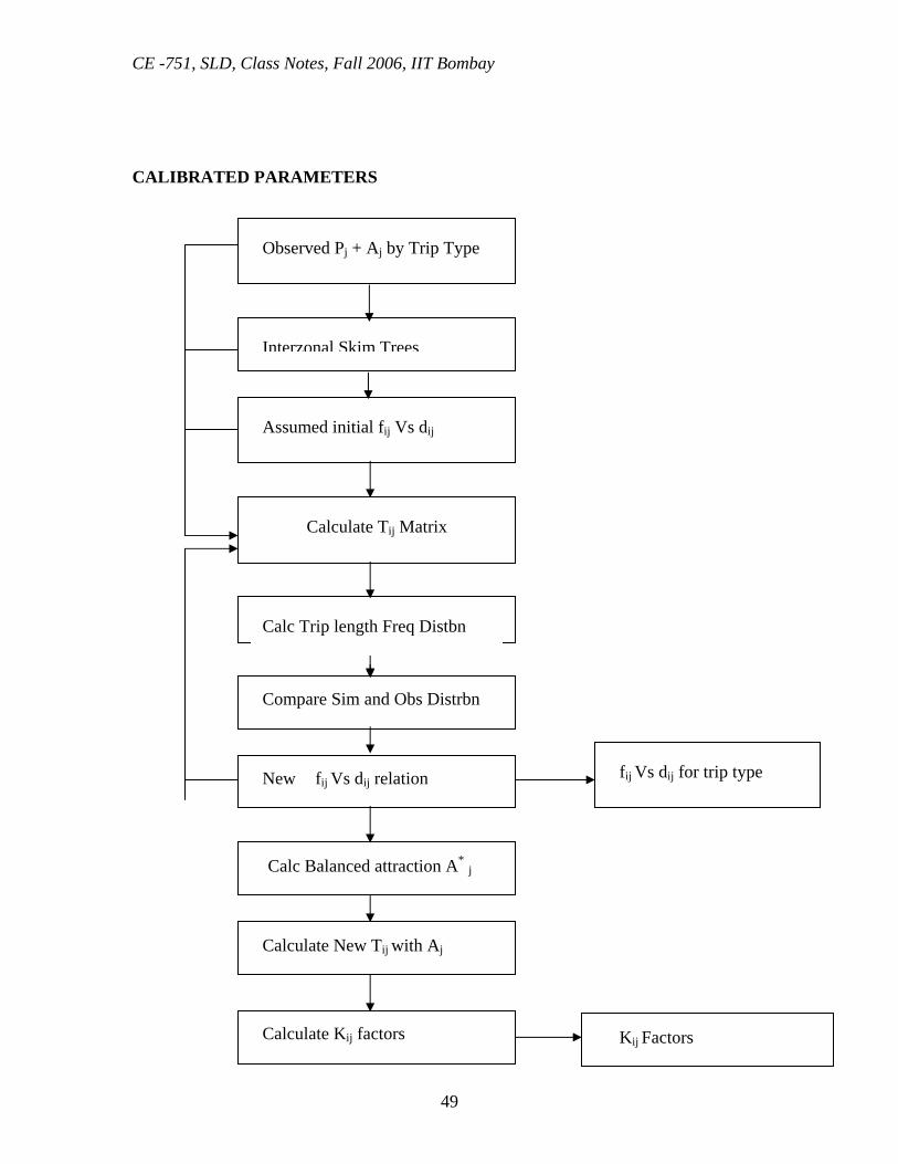
CALIBRATED PARAMETERS
Observed Pj + Aj by Trip Type
Interzonal Skim Trees
Assumed initial fij Vs dij
Calculate Tij Matrix
Calc Trip length Freq Distbn
Compare Sim and Obs Distrbn
New fij Vs dij relation
Calc Balanced attraction A* j
Calculate New Tij with Aj
Calculate Kij factors
fij Vs dij for trip type
Kij Factors
CE -751, SLD, Class Notes, Fall 2006, IIT Bombay
50
The final phase of BPR calibration is to calculate zone to zone adjustment factors
kij.These factors are calculated from the following expressions:
kij = rij [(1-xij)/(1-xirij)]
where kij = the adjustment factor to be applied to movements between zones I and j.
rij = the ratio tij (o-d survey)/tij (gravity model)
xij = the ratio tij (o-d survey)/pi
The final gravity model simulated trip interchange matrix is given by
tij = pi [ (aj*fijkij)/ ∑a j
*fijkij ]
An horizon year trip interchange matrix is calculated from the given equation with the
following inputs:
(1) The horizon year trip production and trip attraction rates,
(2) The horizon year intercentroids skim trees.
(3) The base year travel time function.
(4) The kij magnitudes that are expected to hold for the horizon year.
Limitation:
The limitation of procedure described is it requires that two criteria be satisfied by a base
year calibration. These two criteria are: agreement between observed and simulated trip
length constraint equation .A principal difficulty wit this calibration procedure is that the
travel time factor function and associated trip length frequency distribution are assumed
to be constant for each zone of a study area.
CE -751, SLD, Class Notes, Fall 2006, IIT Bombay
51
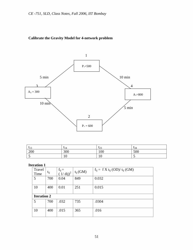
Calibrate the Gravity Model for 4-network problem 1 5 min 10 min
3 4
10 min 5 min 2 t13 t14 t23 t34 200 300 100 500 5 10 10 5 Iteration 1 Travel
Time tij fij = ( 1/ dij)2 tij (GM) fij = f X tij (OD)/ tij (GM)
5
700 0.04 849 0.032
10
400 0.01 251 0.015
Iteration 2 5
700 .032 735 .0304
10
400 .015 365 .016
A3 = 300
P1=500
A3=800
P2 = 600
CE -751, SLD, Class Notes, Fall 2006, IIT Bombay
52
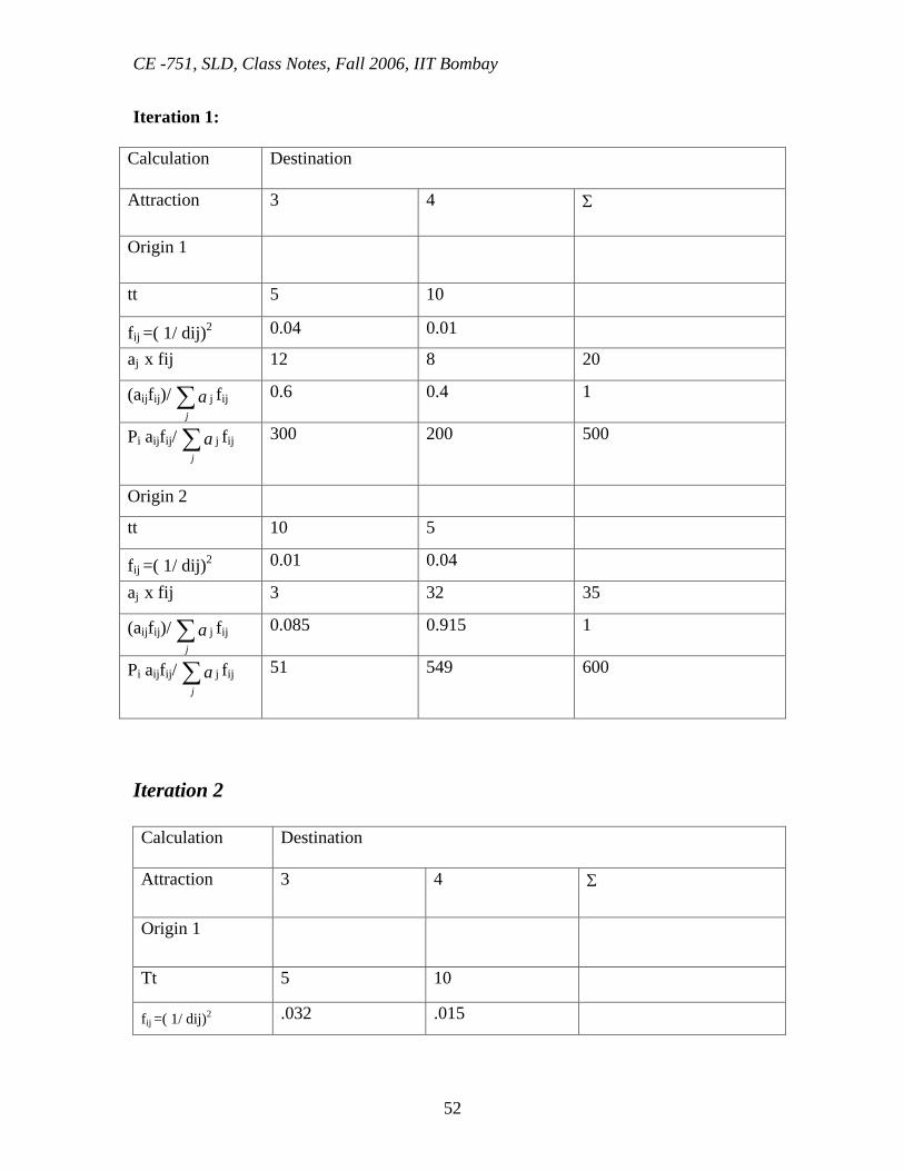
Iteration 1:
Calculation
Destination
Attraction 3 4 Σ
Origin 1
tt 5 10
fij =( 1/ dij)2 0.04 0.01
aj x fij 12 8 20
(aijfij)/ ∑j
a j fij 0.6 0.4 1
Pi aijfij/ ∑j
a j fij
300 200 500
Origin 2
tt 10 5
fij =( 1/ dij)2 0.01 0.04
aj x fij 3 32 35
(aijfij)/ ∑j
a j fij 0.085 0.915 1
Pi aijfij/ ∑j
a j fij
51 549 600
Iteration 2 Calculation
Destination
Attraction 3 4 Σ
Origin 1
Tt 5 10
fij =( 1/ dij)2 .032 .015
CE -751, SLD, Class Notes, Fall 2006, IIT Bombay
53
aj x fij 9.6 12 21.6
(aijfij)/ ∑j
a j fij 0.45 0.55 1
Pi aijfij/ ∑j
a j fij
225 275 500
Origin 2
tt 10 5
fij =( 1/ dij)2 0.015 0.032
aj x fij 4.5 25.6 30
(aijfij)/ ∑j
a j fij 0.15 0.85 1
Pi aijfij/ ∑j
a j fij
90 510 600
LOW’S METHOD Basic Concept: In this model volumes are determined one link at a time, primarily as a function of the
relative probability that trips would use one link in preference to another link. First trip
probabilities are determined for every combination of origin and destination zones in the
area.
The probability of a trip between zone I and zone j can be linked to the gravitational pull
of two masses and the distance separating them as
2
*
ij
ji
dmm
Considering home work trip if mass at home end as employment Ej ,then the trip
probability becomes mij
ji
tEP
Input Information
The Low’s model needs the following information
CE -751, SLD, Class Notes, Fall 2006, IIT Bombay
54
1. Pattern and intensities of land use development now and as anticipated in the future.
This should include population and employment by zone etc but there will be of no
values unless reasonable estimates of future patterns and intensities of land estimates
of future patterns and intensities of land use development can be made in similar
detail.
2. Transportation network characteristics including network configuration, link speeds
etc. 3. Representative traffic volumes from ground count throughout the network. 4. Volume and Patterns of trips with one or both ends outside area under study.
Formation and Use of the Model Current external volumes: Current external trip data gathered in the road side interview survey are first assigned to
the existing network to produce estimates of current external volumes throughout the
network.
Current Internal Volume: These volumes on links throughout the network are computed by subtracting the assigned external traffic volumes from the corresponding ground counts. Internal Volume Forecasting Model: Inter zonal trip opportunity matrices of the form Ai and Bj are developed Where A and B
are parameters that are logically related to trip productions and attractions. Using Travel
time as the measure of separation the friction factor can be expressed as 1/ tm ij
The product Fnij= Ai Bj / tm ij is called inter zonal trip probability matrix. The probability
matrices are then assigned separately to the current network just as if they were trips.
Multiple regression techniques are used to develop equation of the following form
nn FbFbFbFbaV +++++= ......3322111

CE -751, SLD, Class Notes, Fall 2006, IIT Bombay
55
Where V is the internal traffic volume on a link
a and b are constants
Fn is the trip probability factor volume as assigned to that link.
Future Internal Volume: Future zonal socioeconomic data are used to develop future trip opportunity matrices and
future friction factors from the future network to be tested are applied to the trip
opportunity matrices to produce future trips.
Advantages of Low’s Method
• They are easily understood and applied requiring only as inventory of present day
trip origins and destinations and estimations of simple growth factors.
• The simple process of iteration quickly produces a balance between postulated
and computed trip ends.
• They are flexible in application and can be used to distribute trips by different
modes for different purposes at different times of the day and can be applied to
directional flows.
• They have been well tested and have been found to be accurate when applied to
areas where the pattern and density of development is stable.
Disadvantages of Low’s Method
• They cannot be used to predict travel patterns in areas where significant changes
in land use are likely to come and the assumption that the present day travel
resistant factors will remain constant into the future is fundamentally weak.
• These models cannot satisfy the requirements modern urban transportation
studies, which are usually designed to cater for conditions of continual and rapid
changes in the pattern of development and the way of life of population generally.