Embed Size (px)
Citation preview
Modulations in the Leading Edges of Midlatitude Storm Tracks
R H Goodman A J Majda D W McLaughlin
SIAM Journal on Applied Mathematics Vol 62 No 3 (Dec 2001 - Feb 2002) pp 746-776
Stable URL
httplinksjstororgsicisici=0036-1399282001122F20020229623A33C7463AMITLEO3E20CO3B2-D
SIAM Journal on Applied Mathematics is currently published by Society for Industrial and Applied Mathematics
Your use of the JSTOR archive indicates your acceptance of JSTORs Terms and Conditions of Use available athttpwwwjstororgabouttermshtml JSTORs Terms and Conditions of Use provides in part that unless you have obtainedprior permission you may not download an entire issue of a journal or multiple copies of articles and you may use content inthe JSTOR archive only for your personal non-commercial use
Please contact the publisher regarding any further use of this work Publisher contact information may be obtained athttpwwwjstororgjournalssiamhtml
Each copy of any part of a JSTOR transmission must contain the same copyright notice that appears on the screen or printedpage of such transmission
The JSTOR Archive is a trusted digital repository providing for long-term preservation and access to leading academicjournals and scholarly literature from around the world The Archive is supported by libraries scholarly societies publishersand foundations It is an initiative of JSTOR a not-for-profit organization with a mission to help the scholarly community takeadvantage of advances in technology For more information regarding JSTOR please contact supportjstororg
httpwwwjstororgSun Jul 15 170510 2007
SIAhI J APPL XIATH 2001 Society for Industrial and Applied Xlathernatics Vol 62 Nu 3 pp 746-776
MODULATIONS IN THE LEADING EDGES OF MIDLATITUDE STORM TRACKS
R H G O O D L ~ A N ~A J ~ I A J D A ~AND D W LICLAUGHLIN~
Abstract Downstream development is a term encompassing a variety of effects relating to the propagation of storm systems at midlatitude We investigate a mechanism behind downstream development and study how wave propagation is affected by varying several physical parameters We then develop a multiple scales modulation theory based on processes in the leading edge of propagating fronts t o examine the effect of nonlinearity and weak variation in the background flow Detailed comparisons are made with numerical experiments for a simple model system
Key words atmospheric science asymptotics
AMS subject classifications 86A10 76C15
PII SO036139900382978
1 Introduction Observations [6 131 establish that midlatitude storrn tracks live longer and propagate farther and faster than traditional theories would predict The midlatitude (20-70) storm track is a disturbance in the atmosphere comprised of a group of eddies which move eastward as a wave packet gaining energy from strong shears which exist at middle latitudes and are responsible for much of the weather we experience A fuller understanding of the rnecha~lisrns responsible for the generation of these storms would be very useful for weather prediction perhaps leading to a significant increase in prediction times
The storrn track consists of a short wave packet containing roughly half a dozen eddies They are formed at the eastern edges of continents where diabatic heating leads to increased instability Sfaximum eddy activity is found downstream in regions of weaker instability This wave packet then travels through the region of weaker instability This is referred to as downstream development IVhile the storm track has a life cycle measured in weeks and may circle the entire globe it is cornposed of eddies whose i~ldividual lifetimes may be only 3-6 days
The mechanism behind the storrn track is the baroclinic instability Solar heat- ing causes a strong equator-to-pole temperature gradient This sets up a density gradient which competes at midlatitudes with the effect of the earths rotation and leads to the thermal wind balance -a vertical shearing of the predominant west- erlies that make up the jet stream The instability associated with this shear the baroclinic instability is responsible for the generation of storms in this region In the region where storm tracks form the underlying atmospheric flow is absolutely unstable which means that localized disturbances may grow zn place unbounded if
the growth is not arrested by nonlinear processes Downstream the atmosphere is
Received by the editors December 29 2000 accepted for publication (in revised form) July 12 2001 published electronically December 28 2001 This work is based on research toward RH Goodmans PhD at the Courant Institute
httpwwwsiamorgjournalssiap62-338297html +program in Applied and Computational hlathematics Princeton University Fine Hall Washing-
ton Rd Princeton NJ 08544 This author was supported during his graduate studies by an NDSEG fellowship from the AFOSR and a New York University 1IcCracken Fellowship Current address De- partment of Llathematical Sciences New Jersey Institute of Technology University Heights Newark NJ 07102 (goodmanDnjitedu)
i ~ o u r a n t Institute of Mathematical Sciences New York University 251 hlercer St New York NY 10012 (majdaGcimsnyuedu dmacOcimsnyuedu)
convectively unstable which means that localized gro~ving disturbances eventually move away and disturbances remain bounded at any point in space These definitions will be made precise in the text
Several phenomena related to storrn track propagation are generally referred to as downstream development including the following observations eddy activity achieves its rnaxirnum downstream of the region of absolute instability and the storm track propagates easily through the downstream region Storm tracks are observed to move faster than would be predicted by envelope equations based on modulations of unstable normal modes This is consistent with observations that dynamics at the leading edge have a dominant effect on the growth of the wave packet and that the group velocity of the propagating wave packet exceeds its phase velocity-so that the packet appears to propagate by forming new eddies at its leading edge
Downstream development has been observed in a number of observational and numerical studies For the southern hemisphere Held and Lee [13] study European Center for Medium-Range JYeather Forecasting (ECIIJYF) data and observe clear examples of downstream developing wave packets These wave packets correspond to storm systems made up of several eddies which rnay circle the globe several times They estimate phase speeds of individual crests and group speeds of entire wave packets The group velocity is approximately five tirnes the phase velocity implying downstrearn development For the northern hemisphere Chang [6] makes similar observations also based on ECSIJYF data Observing such structures is Inore difficult in the northern hemisphere where there are more land-sea interfaces and the storrn track is less stable
In a collection of 1993 papers [ 5 6 181 Chang and Orlanski observe downstrearn development in numerical experiments for a three-dimensional primitive equation model This model together with simpler models they also study consists of a steady flow containing a vertical shear and usually a jet structure in the meridional direction to model the jet stream They identify and quantify mechanisms by which energy flows toward the downstrearn end of the wave packet causing new eddies to develop They compute an energy budget and find the relative strengths of the various energy fluxes at different points of the wave packet At the leading edge the energy trans- fers are dominated by an ageostrophic flux term This energy flux is due to lznea7 terms in the perturbation equations which describe the evolutio~l of the storm track when the average state of the system is imposed externally They also note that in numerical experiments waves which are seeded in a region of absolute instability are able to propagate easily through a region of convective instability and that the only constraint on the distance of propagation is the size of the channel they study
Held and Lee [13] study a series of models of increasing simplicity an idealized global circulation model a two layer primitive equation model and a two layer system of coupled quasi-geostrophic equations In all cases they see the signs of downstream development Significantly they find that their simplest model the two layer quasi- geostrophic cha~l~lel with the earths rotation and curvature modeled by the 3-plane approximation produces downstream developing wave packets They show that their wave packets fail to satisfy a typical nonlinear Schrodinger description that might be derived from a normal-mode expansion and suggest that an envelope equation description of their wave packets might be very interest~ng
Swanson and Pierrehumbert [23] numerically study a similar two layer quasi- geostrophic system perturbed about a jet-like shear flow They initialize a wave packet centered on the linearly most unstable normal mode Initially this normal
748 R H GOODMAN A J hlAJDA AND D W MCLAUGHLIN
mode dominates the evolution but at longer times leading edge modes dominate the evolution propagating essentially decoupled from the ~ lo~l l i~ lear processes a t the rear
We will explore the interaction between the leading edges of storm tracks and a slowly varying shear flow Some other studies of the baroclinic instability in a variable environment have focused on local and global modes for baroclinically unstable media (Merkine and Shafranek [16]) These are basically eigenmode analyses which apply a linear theory throughout the domain As the studies by Held and Lee [13] and Swanson and Pierrehumbert [23] show that linear theory is dominant only at the leading edge we do not follow the global mode approach
We derive an envelope approximation of the type suggested by Held and Lee but centered on waves with complex wavenumber which dominate the linear leading edge behavior Others have constructed such a theory for unstable normal modes such as Pedlosky [19] and more recently Esler [9] The physical relevance of such a constructio~l is questionable because well behind the front the solution is large and thus no~lli~lear are large as well The only place where the solution i~lteractio~ls is small enough to apply weakly nonlinear theory is in the leading edge and thus it is in this restricted domain where an envelope approxirnation is rnost likely to apply Moreover it is in this very region where the mechanisms of downstrearn development are active Thus we design our asymptotic construction for this region We note that the wavenumbers which are dominant at the leading edge of a wave packet are not necessarily the same as those which dominate the wave packet toward the rear as seen in the numerical experiments of Swanson and Pierrehumbert [23] as well as in analytic studies i~lcludi~lg those of Briggs [2] and Dee and Langer [7]
This study addresses two issues First we examine the effects of varying several physical parameters notably the 0-plane effect and the width of the channel in which the wave propagates on the speed and wave~lurnber of the leading edge front solutions lye then derive a general set of envelope equations that describe the behavior of the leading edge front solutio~ls to PDEs with slowly variable media which we use to model the fact that the atmosphere is absolutely unstable where storm tracks develop but convectively unstable downstrearn We apply these methods to derive amplitude equations for the leading edge fronts of storm tracks in different physical parameter regimes when the shear flow is allowed to contain spatial variation lye also discuss the effects of varying the parameters on the solutio~ls obtained
In section 2 we introduce the model equations describing winds at midlatitudes We discuss mathematical methods used to obtain information about the leading edges of waves in unstable media and apply these methods to our model system examining the effect of the various physical parameters separately and together In section 3 we examine the effect of slowly varying media on the leading edges via a multiple scales expansion which results in modulation equations for the leading edges of storrn tracks under varying physical parameters Finally in section 4 we perform numerical experiments to verify the validity of the modulation equations on a simpler set of model equations
2 Linear leading edge theory for baroclinic systems
21 A mathematical model for midlatitude storm tracks lye begin with the simplest physical model shown by Held and Lee [13] to capture the phenome~lo~l of downstream development Although the Charney rnodel is the considered the least cornplex systern to accurately capture the full dispersion dynamics of the midlatitude baroclinic instability [lo]we choose to work with a simpler two layer rnodel in order to further develop the theory to handle weak variations in the rnedium in section 3
749 MODULATIONS OF AThlOSPHERIC WAVES
We consider a fluid idealized to two shallow immiscible layers of slightly different densities bounded above by a rigid lid at height D The system is in a rapidly rotating reference frame with a variable rate of rotation given by
where y is the (dimensional) distance in the meridional direction to model the cur- vature of the earth (This linear variation of the rotation rate along the meridional direction is derived as a first order approximation to the local normal component of the earths rotation in a small band centered at middle latitude) We include a drag term to model dissipation at the earths surface proportional to r1 times the lower layer velocity We choose the physical scales [LD LU U D U L ] for the horizon- tal coordinates the vertical coordinate time and horizontal and vertical velocities Then assuming the Rossby number Ro = U f o L to be small which indicates a bal- ance between gravitation and the effects the earths rotation we have the standard quasi-geostrophic potential vorticity equations
(+$ 2) =O- (AQl + F ( Q 2 - 8 1 ) + R y )
+ 2(1) ( - (AQ2+ F(Q1 - 8 2 ) + Ry) + r A 8 2 = 02) The nondimensional parameters which appear are
The functions Q1 and 9 2 are the upper and lower layer stream functions so the velocity in each layer is given by
For co~ls ta~l t uj = U j one has the exact solutio~l
a constant zonal flow in each layer A full derivation of these equations is given in [20] We will be concerned with this system in two idealized geometries in the first
the domain is unbounded in both dimensions In the second the fluid is confined to a channel of finite width in the meridional (y) direction and of infinite extent in the zonal (x) direction In this second case we have the boundary conditions
We write perturbation equations by letting
750 R H GOODhIAN A J MAJDA AND D W MCLAUGHLIN
and by letting
be the barotropic and baroclinic parts of the background flow respectively The perturbation equations are
Equations (3) are in dimensional variables with all parameters explicitly repre- sented in the equations We begin by rescaling the equations to reduce the number of parameters We make the scalings
and change variables to the moving reference frame
which makes the mean velocities in each layer u1= 1 and 0 2 = -1 and allows us to work with a system in only three parameters 3 r and the no~ldime~lsional channel width (Note that working in a reference frame moving at the mean velocity oT is equivalent to working in a system with zero mean flow)
lye drop the tildes and obtain the dimensionless equations dependent only on the parameters 3 and r
a1-+ -+ -- ---at a
ax a ayl
a x a y a
a)a y a x (Awl + (yz- W I ) ) + (3+2)-ax = 0
We may write this system as a general differential equation consisting of a linear and a quadratic part
LlODULATIONS O F AThlOSPHERIC WAVES
where in ( 5 )
For the asymptotic methods that follow we require that the linearized version of (6) be unstable in the sense we now describe in section 22
22 Derivation of marginal stabilityleading edge speed We describe a method for finding leading edge marginal stability velocities for linear waves-as put forward by Briggs in [2] and well summarized in Huerre and Monkewitz [14] This is based on linear processes in the leading edges noting that Orlanski and Chang [18] found lznear ageostrophic flux terms to be the dominant mode of energy transfer in simulations of downstream developing baroclinic systems and that Swanson and Pierrehumbert [23] found that propagation is controlled by leading edge dynamics
Consider a y-independent linearized form of our generalized equation (6)
where C is a matrix valued polynomial in two variables This has solutions of the form
for w and k satisfying the dispersion relation
(9) A(k w) = det C ( k w) = 0
The general solution to (7) is given by a space-time convolution with Greens function which satisfies
G(x t ) may be represented by a Fourier-Laplace integral
where r the Bromwich contour is a horizontal line in the complex plane lying above Imw = a Cj are the entries of the matrix Cand
This choice of r ensures causality by allowing the w-integral to be closed in the upper half plane for t gt 0The leading term of the asy~nptotics for t gtgt 1 will be given by
752 R H GOODMAN A J MAJDA AND D W MCLAUGHLIN
where the quantities k w and v are defined in the discussion below We will study the asymptotic behavior of solutions as t -+ along the ray
x = xo + ut We will first show how to find the local growth rate in the reference frame u = 0and then show how to extend this argument to a moving reference frame with velocity u 0We fix x = xo and study the behavior of solutions as t -+ x First we evaluate the k-integral For xo gt 0 the Fourier contour must be closed in the upper half k-plane For each on the Bromwich contour we define the pole loci as
The pole loci then determine the singularities of the integral (11) If A(w k) is N t h degree in k then for each w on the Bromwich contour the pole loci contain N roots the first N+ of which lie in the upper half plane The k-integral in (11) can then be evaluated by residues
To evaluate the remaining integral for large t the Bromwich contour r should be deformed downward as far as possible in the complex w-plane The asymptotics are then dominated by the singularity in the w-plane with the largest imaginary part Note however that the pole loci are defined in terms of the w-contour and shifting r also causes the pole loci to shift When r lies entirely above the line Imw = a then the pole loci do not intersect the real k-axis as a is the maximum imaginary part of w for any k on the real axis As r is shifted downward below this line however the pole loci may intersect the real k-axis on which the Fourier integral is performed Thus as r is deformed the k integration contour must be deformed to avoid the singularities of this integral As the k-contour is deformed the pole loci also deform For critical values of w two branches of the pole loci may coalesce This deformation process is shown in Figure 21
When two poles on the pole loci coalesce one of two things may happen If two pole loci from the same side of the k-contour coalesce they will not contribute to the integral as two coalescing first order poles form a pure second order pole which has zero residue If two poles from loci on opposite sides of the k-contour coalesce then the k-contour is pinched between the pole loci and r can not be lowered any further Let w be the uppermost point in the +plane for which two pole loci cross from opposite sides of the Fourier contour and let k be the point in the k-plane where they cross Clearly where two pole loci coalesce the dispersion relation (9) must have a double root so that
dA -(k w) = 0dk
Thus finding a saddle point of A(k w) is a necessary condition for finding the dominant term in the asymptotics but not a sufficient one as the double root must arise from a pinching of the Fourier contour between the pole loci
Note that as (k w) -+ (k w) the denominator in (13) goes to zero so that the integral is singular at this point To evaluate this integral asymptotically we expand
FIG 2 1 To asymptotzcally evaluate the double zntegral over the Bromampzch contour r and the Fourzer contour F zn ( a ) the contour r zs shzfted doampnward (b) amphzch requzres a shzft of F untzl a szngularzty zs met ( c ) and F becomes pznched between the zmages of r zn the k-plane Thzs figure zs reproduced from [14]
it in the neighborhood of the singularity (14) Repeated use of Taj-lors theorem yields
the sign of which will depend on the specific problem The denominator in (13) thus vanishes as (w- d ) and the leading term of the integral in (13) may be obtained from the expansion about this singularity
754 R H GOODMAN A J MAJDA AND D W MCLAUGHLIN
The exponential growth rate in the stationary frame is thus given by eIrnu5We may extend this analysis to find the growth rate in a reference frame moving at constant velocity v by considering the behavior as t -+ with x = xo + vt This is equivalent to a change of variables to ( 2 = x - vt f = t ) We repeat the preceding analysis in this frame with iZI = w -vk and = k The growth rate in the reference frame moving at constant velocity v is thus given by eImGs= elm(Ws-vks)The dispersion relation is independent of the moving reference frame while the saddle point condition can be written in the original variables (k w) as
Suppose that there exists a finite range of velocities (vt vl) such that the growth rate Imil(v) is positive for reference frame velocities in this interval and vanishes at the endpoints vt and vl These velocities define a wave packet which is both expanding in space and growing in amplitude The trazlzng edge speed will be given by vt and the leadzng edge speed will be given by vl These are referred to as marginal stability velocities because they mark the transition between reference frames in which the solution is growing to those in which it is decaying We will denote the leading edge marginal velocity by v and the associated wavenumber and frequency in that reference frame k and w The marginality condition can be written as
(17) ImG = Im (w - vk)= 0
An unstable system is deemed absolutely unstable if 0 E (vt vl) that is if the growth rate in the stationary frame of reference is positive In this case a localized disturbance will eventually grow to overtake the entire domain By contrast it is conuectiuely unstable if v = 0 is not contained in the region of instability In this case a growing disturbance will eventually move out of any compact region and the limiting solution is finite a t every point in space We will use the methods described here to discuss the absolute and convective stability properties of the background shear flow at midlatitude
To summarize the asymptotic properties of the leading edge wave will be de- scribed by the triplet (v k w) which satisfies
(18) A(w k) = 0 the dispersion relation
the saddle point condition
(20) Im(wf - vk)= 0 the marginality condition
in addition to the more stringent conditions that the saddle point arise as a true pinch point and that this be the largest v for which such a triplet exists
23 Numerical implementation of this method For a complicated system of PDEs the three preceding conditions will not be solvable in analytic closed form so a numerical scheme must be implemented to find the leading edge speed We accomplish this in two steps First with v as a parameter we find all ordered pairs (k w) which satisfy the dispersion relation and saddle point condition (18) and (19) and we determine which of these represent pinch points and thus contribute to Greens function The second step determines the growth rates associated with these wavenumbers and looks for the edges of the stability regions in velocity space to determine the leading edge speed
755 MODULATIONS OF ATMOSPHERIC WAVES
Our first step is to find all the saddle points of the system We may eliminate the d from the pair of equations by forming the resultant of the two polynomials (18) and (19) when considered as functions of d [3] This forms a higher order polynomial in k alone This is advantageous for two reasons First we may simply read from the degree of this polynomial how many common roots are shared by (18) and (19) Second we may use iterative eigenvalue methods to find the roots of a single poly- nomial This method was found to be much more stable and reliable than using a Newton method to jointly solve the system of two polynomials
To find the leading edge properties of the wave first the resultant is found sym- bolically using IIaple Then all the roots k of the resultant are found nunlerically as a function of the reference frame velocity z t For each of these k the accompany- ing frequency w and growth rate Im(d - r k ) are formed Each root k which gives a positive growth rate is then examined to see if it corresponds to a pinch point and contributes to the asymptotic solution Note that a double root is a pinch point if the two pole loci which join to form the double root are on opposite sides of the Fourier contour before the Broinwich contour is lowered Therefore we may simply examine where the two roots go if the imaginary part of d is increased to othe maximum growth rate for real wavenumbers If one root moves to the upper half k-plane and the other root irioves to the lower half then the double root corresponds to a pinch point
We then examine the growth rates Im(w - ck) of all the growing modes as a function of velocity and find a region of instability with respect to the reference frame velocity u The velocity at the right endpoint of the instability region is then taken to be the leading edge marginal stability velocity c
24 Application to downstream development R e now consider the scaled two layer midlatitude quasi-geostrophic equation (5) and we consider leading edge dynamics with or without $-plane and lower layer Eknlan drag effects We will look primarily at flows with no dependence on y the cross stream direction and then generalize to flows in channel geometries
241 The inviscid f-plane no channel R e first present the simplest possi- ble variant of the above system by setting the Coriolis parameter $ and the coefficient of Ekman damping r to zero and assuming a y-independent geometry IVe will be able to gain a complete understanding of this system and then may consider the fuller versions perturbatively We also discover some bifurcations as the parameters are varied which demonstrates the limitations of the perturbative approach
lye linearize the scaled perturbation equations (5) with 3 = 0 and r = 0yielding
If we look for sinusoidal normal-mode solutions of the form (8)then (wk ) must satisfy the dispersion relation
R H GOODMAN A J MAJDA AND D W LICLAUGHLIN
F I G 22 T h e selected wavenumbers as a function of reference frame veloczty There are eight waves selected i n each reference frame labeled 1-8
Thus the disturbances of wavenumber k 2 lt 2 are unstable The saddle point condi- tion (19) in the reference frame moving at velocity L is given by
Eliminating w between (22) and (23) yields
Thus implementing the procedure described in section 23 solving this final equation with z as a parameter gives us a set of eight candidate wavenumbers Figure 22 shows the selected wavenumbers as a function of the reference frame velocity 1Only those with Im k gt 0 are relevant in the leading edge of a disturbance as the solution must decay as x + +m
Figure 23 shows the growth rates for the four right-decaying wave solutions The two roots labeled 1 and 2 in Figure 22 which diverge to cc as 214 1 do not satisfy the pinch point condition so do not contribute to the integral
The point where the last curve crosses the axis is the marginal reference velocity and is marked with a star in Figure 23 For this system the leading edge speed may be found exactly The critical velocity is v = 4At this velocity the coefficients of k2 and k6 in (24) vanish so that (24) becomes
which may be solved by the quadratic formula The two roots k = i l + i represent the exact wavenumbers making up the leading edge of the wave The leading edge
757 MODULATIONS OF AThlOSPHERIC VAVES
FIG23 The growth rate of the waves which are right-decayzng as a function of reference frame velocity A star marks the speed v = 4at whzch the system is neutrally stable
properties are thus given by
We may use this analysis to clarify a point made by Merkine in [15]He finds that IUTI lt filUBI is a necessary and sufficient criterion for absolute instability Recall that we have chosen UT = 0 and UB = 1 If UT and UB are chosen generally then the leading and trailing edge velocities are c = UT ~ U B = - filt 0If 21- UT then the system is absolutely unstable which is Merkines condition
242 The addition of the P-plane effect Djext we investigate the effect of reintroducing the 3-plane terms into the equations IVe linearize the scaled perturba- tion equations ( 5 ) with 3 gt 0yielding
Again we substitute the ansatz (8) and find the dispersion relation
We may solve the dispersion relation for d with real k
R B GOODMAN A J MAJDA AND D W MCLAUGHLIN
F I G 24 The wavenumbers representing the six roots of the P-plane resultant which are not present i n the f-plane model Solid lines denote posztive imaginary parts dashed curves denote negatzve imagznary parts
and find that this may give growing normal modes if 3 lt 2 (It is more standard t o write the condition for instability in terms of a critical shear UB [19] which we have scaled to equal one) The f-plane system is unstable for any velocity so the 0-plane effect stabilizes the background shear flow
IVe find that k now satisfies a polynomial of degree 14 yielding 14 possible values of k for each 2) For the f-plane equations there were only 8 roots so 6 new roots arise when 0 is increased from zero The six new waves are shown in Figure 24 for the case 3 = 01 The structure remains very similar as 3 is increased Our initial expectation was that the leading edge speed for small 3 would be a small perturbation of the leading edge speed for of the f-plane equations The new roots instead change the behavior dramatically
For small values of the new roots and the old roots seem to behave indepen- dently of each other The roots relevant to the leading edges are labeled 9 and 14 in Figure 24 These are not simply perturbations of the roots which give the leading edge for the f-plane equations They display an interesting and unexpected behavior At a specific value of c to the right of the marginal point for the f-plane equations two pairs of conjugate roots coalesce at a finite 21crltlcal and for c gt ~ ~ ~ ~ ~ ~ lhave zero imaginary part This bifurcation point which corresponds to the largest marginal stability velocity is clearly visible in Figure 24 The Briggs procedure fails as the leading wave behavior is given by a nongeneric higher order saddle point correspond- ing to a quadruple root of the dispersion relation (27) Therefore Z1 ( k )= 0 Briggss asymptotic formula (12) does not directly apply
As 4 0 the resultant factors into the degree 8 f-plane resultant and a second
759 hlODULATIONS OF ATMOSPHERIC WAVES
polynomial of degree 6 From this second polynomial we may find a perturbative value of the leading edge wavenumber and find that the associated leading edge velocity
approaches t t = d s which is very close to the numerically obtained values for finite 3 and nearly three times the speed predicted for the f-plane This contrasts sharply with the results of studies that include realistic vertical structure for which the nonzero 3 causes a net decrease in the leading edge speed [ 2 2 ]
243 The addition of dissipation Kext we reintroduce dissipation in the form of lower layer Ekman damping which will remove the degeneracy discussed in the previous section The PDE is given by
The dispersion relation becomes complex and the resultant equation in k alone is a complex coefficient fourteenth degree polynomial and the roots no longer occur in conjugate pairs Dissipation has the expected result of breaking the degeneracy of the leading edge mode arid slowing down the leading edge speed slightly Recall that for the conservative equation a pair of conjugate roots bifurcates to a pair of real roots at the leading edge speed zl Figure 25 shows that when dissipation is added the bifurcation no longer takes place The structure of the bifurcation remains visible in the perturbed system The selected wavenumber however has an imaginary part of about 10W2 so that the basic shape of the leading wave remains sinusoidal when dissipation is added with only a very slow exponential decay Figure 26 shows the stabilization and the decrease in the speed of the leading edge resulting from the dissipation It also shows that the growth rate levels off after crossing the marginality point and does not continue to decav quicklv as was the case for the f-plane leading edge A more robust rnodification to the leading edge properties will be given by the addition of a channel geornetry For later reference we present a table of the values at the leading edge with J = 16 the value used by DelSole 181 under our nondimensionalization and r variable
(29)
244 The effect of the channel geometry The discussions above have all focused on y-independent geornetries which we a-ill use to exarnine how y-independent fronts are modulated in the presence of slowly varying media AIany other instability studies [89 15 191 foclis on channel geornetries where the fluid is bounded between hard walls a t y = 0 and y = L UTe examine the effect of the channel width both on the leading edge of the f-plane equations and the more interesting changes that take place in the high order rnultiple root which characterizes the leading edge for the equations
245 The f-plane equations The normal-mode solutions to the linearized equations are
(t) = () e z ( k x - d t ) sin y
R H GOODMAN A J MAJDA AND D W MCLAUGHLIN
No Dissipation Nonzero Dissipation
04
025 025
-0 1 2 3 4 5 0 1 2 3 4 5
v v
F I G 2 5 The breaking of the bifurcatzon for the leading edge wave
FIG26 The growth rate versus velocity for the dzssipative (solid line) and zero disszpation (dashed line)
MODULATIONS OF ATMOSPHERIC L W E S 761
FIG27 Marginal stabzlzty velocity vs y-wavenumber 1 showzng good agreement between the values computed vza the perturbatzon expansion (+) and vza the numerical procedure (0)
a-here 1 = FYe shall take N = 1as this mode is the most unstable The dispersion relation is
As before the formula for selected ivavenumbers is of fourth degree in k2 A wide channel gives rise to a srnall wavenumber 1 = t which admits the pertur-
bation expansion
The perturbation series gives excellent approximations to the values of the leading edge velocity as shown in Figure 27 Slerkine [15] finds bv a formal argument that the condition for absolute instability of this system is given by UB gt f i ( 1 - $) I2 which agrees with the perturbation series to leading order
246 The P-plane equations in a channel In this section tve investigate the effect of the channel geometry on the high order root tvhich determines the leading edge wave for the 3-plane system The effect is more dramatic than of simply adding
R H GOODLIAN A J MAJDA AND D W LICLAUGHLIN
F I G 2 8 Growth rate versus veloczty wzth 1 = 1 (solzd) 1 = 25 (dashed) and 1 = 4 (dash-dot)
dissipation DelSole in [8]studies the 3-plane equations in a channel and does not shot$ a high order root a t the leading edge This leads us to studv whether the channel geometry is sufficient to remove the degeneracy
We study the 3-plane equations with 7 = 0 and find that k satisfies a polynomial equation of degree 16 We fix 3 = 16 corresponding to the value used in [8]and decrease the channel width from xwhich is equivalent to increasing 1 from zero The system goes through three stages (i) When the channel is very wide the behavior is essentiallv the same as for a channel of infinite width (ii) As the channel is nar- rowed however a second high order root forms at a velocity greater than The1 1
two quadruple roots move together as the channel is narrowed further and at some critical channel width annihilate each other (iii) Beyond this value the multiple roots disappear and the svstem contains no degeneracy In Figure 28 the growth rate is shown as a function of velocity for values of 1 in the three above regimes (i) When 1 is small the behavior is the same as when 1 = 0The leading edge wave bifurcates a t some finite value of I beyond which there is no pinch point (ii) For intermediate 1 there exist two critical velocities separating two unstable wave packets (iii) For 1 sufficiently large these two critical velocities and hence the associated wave packets merge and the leading edge wave is determined by a double root as in the standard Briggs procedure Such an 1 corresponds to a channel whose width is two to three tirnes the tvavelength in the zonal direction
This shows that the multiple root which appeared to determine the leading edge behavior is an artifact of the one-dimensional geometry However even without this degeneracy the leading edge speed is significantly enhanced in the presence of nonzero 3
763 hIODULATIONS OF AThlOSPHERIC WAVES
3 Modulation by nonlinearity and weakly variable media With the description of the marginally stable linear wave front in hand we now examine the effects that nonlinearity and weak variation in the background shear flow have on downstream developing dynamics Recall that the atmosphere is absolutely unstable off the eastern shores of continents and convectively unstable over the oceans An easy way to model this is to allow the strength of the shear to vary slowly To create a variable medium we linearize (1) about the (nearly) exact solution
This is not an exact solution to (1)but we may think of it as arising due to a balance of unwritten damping and driving terms in the equation
JVe again consider the quasi-geostrophic potential vorticity equations as given in the abstract form (6) We further assume that the solutions depend only weakly on the transverse y direction through a scaled variable Y = ay We therefore write as a generalization of (6)
where for the quasi-geostrophic equations with shear flow as given in (33)
and
To study how the leading edge wave is slowly modulated by the additional terms in this equation we develop a multiple scales expansion centered around the y- independent leading edge mode e ( ~ - - ~ )b If we assume that the solution is in- dependent of y to leading order then the only y-dependence in the solution will be generated by the variable coefficient term M
JVe follow the standard procedure in deriving envelope equations with one major exception we center our asymptotic expansion on the linear fronts described in the previous section instead of on normal modes A normal-mode expansion requires a weak instability so that the leading order term in the expansion can be approximated by a neutrally stable mode By using the linear front we are able to carry out the expansion for strongly unstable systems by working in the reference frarne moving with the front A major side effect of centering our expansion on these fronts is that nonlinear terms will not enter our envelope equations even if nonlinearity is present in the system The form of the asynlptotics will show that this method is applicable only if the variable coefficient term M satisfies certain restrictions
11-e recall that a multiple scales expansion to a PDE consists of expanding both the solution and its derixatives in powers of small parameter 6 and solving a sequence of equations at increasing powers of 6 The nlodulation equations are then derived as the result of solvability conditions for these equations necessary to preserve the assumed ordering of the expansion Ye write
764 R H GOODMAN A J hlAJDA AND D W MCLAUGHLIN
where is the linear leading front slowly modulated in space and time + q ( l ) = A(ltYT2)ge(k-t)
and the first correction is given by
where X Y and Tl are C(E) slow space and time variables T2 is an 0 ( t 2 ) slow time variable and 6 is a slow space variable in the reference frame moving with the front The terms and $(22)arise due to the nonlinearity The result of the $ ( 2 1 1 )
asymptotics derived in section 31 may be summarized as follows Asymptotic result If $(lo and $(2) are defined as above then the correctaon
t e r m B zs of the form B = O ( X T I Y ) A ( J YT 2 ) and A and O satasfy
(36a) O T ~+ VOX= m ( X Y )
T h e coef icients m and p are given below in (45) and (46)
31 The leading edge perturbation expansion In this subsection we de- rive the results in (36) LYhen the solution is sufficiently small of order E or smaller then will approximately satisfy the linearized equation Since the front decays exponentially the solution will certainly be sufficiently small for sufficiently large x
We define slow time and space scales
X = E X Y = t y T I = t t and T2 = t 2 t
and expand the derivatives accordingly
d d d d d d d -+ -+t - and -+ - + ~ - + ~ 2 -d x ax ax dt a x dTl dT2
We assume that the solution depends on y only through the slow variable Y so that
The leading order equation is taken to be a slow modulation of the leading edge wave 4
(37) d ( l )= + CCA ( X YT I T2)ez (kx-wt )g
where CCdenotes complex conjugate Recall that we may form the matrix L ( k d )
from the relation
~ ~ ~ ( k x - w t ) gL (k w) e ~ ( k x - ~ t ) g=
The vector 6 must be in its null space so we may without loss of generality set
765 hlODULATIONS OF ATMOSPHERIC WAVES
We plug in the multiple scale ansatz and separate orders to derive a formal sequence of equations of the form
where the derivatives of are evaluated at the point (k d ) We see that (39) and (40) are of the form
Thus we must solve this class of linear equations First we define a resonance as a forcing term on the right-hand side which causes the solution to grow to violate the ordering (35) for large t (The solution (I) is meaningful in the reference frame moving at the leading edge velocity so it is in this reference frame we must evaluate the asymptotic ordering) By the Fredholrn alternative a resonance will occur if is in the adjoint null space of C
Nonresonance assumptzon We make the standard assumption that C is a dis- persive operator in that d l ( k ) 0 so that if a particular wavenumber and frequency satisfy the dispersion relation A ( k d ) = 0 then in general nlultiples of the ordered pair (nk n d ) will not also satisfy the dispersion relation ie A(nk nd ) 0 In fact we will make the slightly more general assunlption that terms on the right-hand side of (41) of the form = oeklx-lt) for (k l d l ) (kd) which arise in the course of this expansion satisfy A(kl d l ) 0 SO that (41) is solvable Fortunately for all the systems we anvestagate the nontianashzng condataon
is satisfied and there is no resonance due to nonlinear terms
311 0 ( e 2 ) The leading order ansatz (37) solves the O(s) equation so we may move to the next order The O(s2) equation then becomes
where we have let d = kx - d t It will be convenient to consider the effect of the linear and nonlinear forcing terms separately
Nonlinear terms The term a(() (I)) in (42) gives rise to terms on the right- hand side proportional to e2 e c 2Irn By the above nonresonance assun~ption these will give rise to terms of the same form in the expression for $(2) In the reference frame moving with the leading edge front these have zero growth rate so are not resonant
766 R H GOODMAN A J hlAJDA AND D W LICLAUGHLIN
Linear terms Given the nonresonance assumption we need consider only the linear portion of (42)
The tern1 on the right-hand side will give rise to resonances unless it is perpendicular to the adjoint null space of C Enforcing this nornlal condition gives the general solvability condition [l11 Changing independent variables to
the amplitude A is seen to depend only on the group velocity variable E
We define for the (E r ) reference frame the wavenumber and frequency
k = k and 2 = u -vk
A (nonunique) solution is given by 2= (ao ) ~ where
and primes denote derivatives with respect to k The condition that the solution decay as x + cc prevents us from including a constant terrn in the general solution We include in our full solution an additional solution to the homogeneous equation which will be used in eliminating resonances due to the variable medium Thus the full solution reads
4
(2) = ((i)+ O(X T1IAg) + ~ 2 2 ) ~ - 2 1 m ~ e t ~ + ~ ( 2 l ) ~ 2 z 0 + cc(43)
where the terms $(211) and $ ( 2 s 2 ) are generated by the nonlinear forcing term B
312 O ( e 3 ) Again we consider the linear and nonlinear terms separately Nonlinear terms The terms on the right-hand side of the forrn B(amp() g(2))
and B((~)$()) will lead to forcing terrns that look like e(kx-wt) and e z ( ( k ~ f 3 z k ~ ) x - ( d ~ f 3 z ~ ) t )as well as terms of the type discussed in the previous section on nonlinear terms By the nonresonance assumption these terms do not contribute to resonances
We note here the effect of centering our asyrnptotics on the leading edge front If the expansion had been performed for nornlal modes then the imaginary parts of k and d would be zero and there would be a forcing term proportional to ez(kx-wt) arising due to the nonlinearity This is precisely how the cubic nonlinearity arises when the nonlinear Schrodinger or Ginzburg-Landau equation is derived as an envelope approximation-a rnechanisrn lacking in this wave front situation
Linear terms As the nonlinear terms do not in general cause resonances the solvability condition for (40) cornes entirely frorn the linear terms and the ordering of the expansion is violated unless
- det [ 1 M (-kll)]A - det [ 1 AYY= 0Cy ( -ampCI2)]
MODULATIONS O F AThlOSPHERIC WAVES
Define
m = i det [ I M A()I We may split (44) in two by taking a derivative with respect to T recalling that A = L + vampAs AT 0 the remaining terms will be aT =
m(X Y)) = 0
This may be integrated once to obtain
with constant of integration F We may solve the O equation to obtain
This explicit formula for O shows that the asymptotic ordering could be violated if m(X Y) is not subject to rather stringent restrictions In general we rnay set F to be
which means this limit must exist for each Y in the donlain considered We then use (48) to eliminate O from (44) yielding
32 The two layer f -plane without dissipation The first rnodel for which we discuss the leading edge rnodulation equations is the inviscid f-plane The nondi- rnensionalization of this model and the determination of the properties of its leading edge linear front are discussed in section 2
The leading order linear operator is discussed in section 241 Recall that the linear part of the front is of the form
where the wavenumber frequency and velocity are given by
To form the coefficients of the two main modulation equations described in (36) we need to compute the following quantities
768 R H GOODMAN A J MAJDA AND D W hlCLAUGHLIN
as well as
det [ i M (-)I and det [ I CYI ()I Substituting the leading edge quantities (52) into the preceding expressions yields
ALL= 16i
A = 8amp(l + i)
det [ i 1 M (-)I = 8(-1 + i (1 + amp))(-V1 + i ( h -
where the coefficients are given in the following table for
Thus the final equations are given by
0 + ampOx = iampVB + (1 - i)VT
where VT and VB are the barotropic and baroclinic parts of the velocity respectively as defined in (2)
33 -plane equation with Ekman drag We are unable to perform this asymptotic expansion for the Bplane equations when I- = 0 due to the high order real root at the leading edge We can however derive amplitude equations when dissipation is included Using the values given in (29) we derive equations of the form
= 16 with r as given in the table
Note the interesting fact that as the dissipation increases in the full equation the diffusion actually decreases in the Y direction as it is enhanced in the 6 direction
4 Numerical experiments Next we confirm numerically the asymptotic pro- cedure described above That the wave moves at the selected speed and has the correct decay properties has been computed by others [7 211 The leading edge speed wavenumber and frequency have been well verified for systems such as we are studying but the challenge in confirming the asymptotics is in resolving the exponen- tially decaying leading edge over several orders of magnitude In addition the slow time scales and long spatial scales imposed by the asymptotic problem require that the numerics be carried out on a large domain for long times While second order methods would certainly be sufficient to verify the basic properties of the unmodu- lated system accurate representation of the modulations due to the weakly varying coefficients over a long domain requires a higher order method
769 hIODULATIONS OF AThIOSPHERIC WAVES
41 Description of numerical experiments To write a code that would implement the atmospheric wave equations to the accuracy needed would be an ex- tremely difficult task so we choose to validate the asymptotics on a simpler model problem-a variable coefficient complex Ginzburg-Landau equation
This equation is often used as a model for the evolution of systems with weak nonlinearities and weak instability [17] and has been derived as a model for the two layer quasi-geostrophic equations by Esler [9] The problem we solve is to set u= 1 at x = 0 with conlpactly supported initial conditions allowing a wave propagate to the right
Although our general derivation of modulation equations was performed for vector systems a similar derivation may be done for this scalar equation For later reference the selected wavenumber frequency and velocity are
42 Numerical difficulties In order to get meaningful results from this nu- merical experiment a code of higher-than-usual accuracy will be needed especially for the spatial discretization To see why recall that the important terms are A and 0where the full solution in the leading edge is of the form
where k and UJ are complex In order to compare theory with the numerical experi- ment we must know A to several decimal places but over the domain of computation u decays from order one down to ~ ( e - ~ ) If standard Fourier methods are used to compute the derivative then the solution can only be resolved down to size 10-l6 in double precision arithmetic We instead use high order methods which are more local in nature which are able to resolve the amplitude of a decaying exponential over greater distances [12]
For temporal discretization there are two competing difficulties which lead us to our numerical method First we have stiffness due to diffusive and dispersive terms in our PDE which would suggest that we use an implicit method Second we have nonlinear terms and we would like to avoid using implicit methods and needing to solve fully nonlinear equations at each step We would also like to be able to use a high order method so as not to squander the accuracy of the spatial discretization
43 Summary of method Briefly our method will consist of a method of lines First we impose a spatial discretization and specify a method of computing approximate spatial derivatives This reduces the PDE to a system of ODES for the vector 6(t)which is then solved by a suitable time stepping method
44 Spatial discretization The spatial discretization is performed by a mul- tidomain Chebyshev collocation due to Yang and Shizgal [24] Generally Chebyshev methods are much more adaptable to boundary conditions than are related Fourier methods lye begin by defining the standard Chebyshev collocation method and then explain the multidonlain version On the interval [-I 11 we define the Gauss- Lobatto-Chebyshev (GLC) points
770 R H GOODhIAN A J LlAJDA AND D Mr LICLAUGHLIN
Let f be a smooth function defined on [-I 11 and let f b e the vector f k = f (xk) of values at the GLC points Then we may compute an approxinlate derivative as
f 1 ( ~ k )= Dfkgt
where [4]
where c = 1 for 0 lt j lt N and co = cAi= 2 and x are as defined in (55) (This comes from representing f as a sum of the first n + 1 Chebyshev polynomials and such a derivative converges faster than any power of N as N + m)
It is not practical to implement this method over a large computational domain as D is a dense matrix and becomes extremely ill conditioned for large values of n Therefore we consider a piecewise method using overlapping subdomains as described by Yang and Shizgal in [24] In this method we partition the interval into overlapping subdomains of equal length so that the last two GLC points in one subdomain coincide with the first two points in the next subdomain If we choose to partition an interval of length L into J subintervals and want to use approximating polynomials of degree N then there will be
total collocation points and the length lSub of the subintervals will be given by
2L lsub = (J f 1) + ( J - l ) c o s
Such a partitioning is shown in Figure 41
The kth subdomain
X0 fi + x x
N-I N 2N-I
F I G 41 Partitioning of a n znterval znto J ouerlappzng subdomazns Ik
If we let D be the ( N + 1) x ( N + 1) collocation derivative operator for a single subdomain with the points in the subdomain labeled 0 through 1Y then the full operator 2) has a nearly block diagonal structure The resulting linear system is nearly block diagonal We may then use this approximate derivative to discretize a boundary value problem which is very efficiently solved by Gaussian elimination using a specially adapted partial pivoting scheme subject to the constraint that two rows may be interchanged only if they are in the same block Such a matrix may
h1
hIODULA4TIONS OF AThlOSPHERIC WAVES
FIG42 T h e vanable coeficzent p used zn one expenment
be factored in O(JN3) steps and the forward and backward substitutions may be performed in O ( J N 2 ) steps The elements of the matrix may be stored in a one- dimensional array consecutively by rows with all the arithmetic done in place with zero fill-in Thus with N fixed quite large systems may be solved very efficiently In practice lZr = 6 was found to be sufficient
45 Time stepping To solve this ODE the right-hand side is split into two pieces one containing all the terms responsible for stiffness and for instability and one containing all the convective and nonlinear terms The ODE may then be written in the form
and solved by a high order splitting algorithm described below The time stepping is done using the implicit-explicit multistep schemes due to
Ascher Ruuth and Wetton [I] These allow us to compute the nonstiff cubically nonlinear terms and advection terms explicitly needing only to solve implicitly for the terms due to the higher order spatial derivatives This may be thought of as a high order splitting method which allows us to avoid costly iterations of a nonlinear solver
46 Results of one-dimensional simulations Recall that the one-dimensional numerical experiments are performed for the model equation
For all experiments reported the parameters used were zt = 3 P = 1 and y = 2 which makes the equation convectively unstable The experiments were performed with sixth order piecewise collocation and a total of 1000 subdomains for 0 5 x 5 1000 A variety of variable coefficient functions p(tx) were used an example of which is plotted in Figure 42 with E = 2This function was generated by a random Fourier sine series Other functions we used for p included Gaussians sinusoids and sums of randomly placed Gaussians The quality of the results was fairly independent of the shape of the variable coefficient as long as the criterion was met that the mean of p was zero
Figure 33 shows a contour plot of the wave spreading to the right at constant velocity vwith the variable coefficient as shown in Figure 32
To postprocess these numerical results in the parallelogram region pictured in Figure 43 we form A(1+ EO) by dividing the full solution by ez(kx - t ) Th is region is defined by to lt t lt t l and xo - vto lt x - vt lt XI - zftl In this region the solution has an amplitude of about ul = 15 at the left edge and about (uJ= 10-l6 at the right edge due to the exponential decay of e Thus we remove this large variation and focus on A( l + euro0)
R H GOODhIAN A J LIAJDA AND D W LICLAUGHLIN
real (u)
F I G 4 3 Solutzon to the PDE spreadzng to the rzght The parallelogram regzon shous the regzon zn ( [ T 2 )varzables where the slowly Laryzng functzons A and O are defined
Next
is formed from p where recall TI = et lt = t ( z - z i t ) This allows A to be calculated from the solution to the full PDE Il-e rnay then cornpare its evolution with that of the envelope equation The initial and boundary values of A are used to nurnerically conlpute the evolution of A under the reduced equation (51) and the results are compared with the values of A obtained frorn the full sirnulation Results are shown in Figure 33 The relative error between the envelope A as cornputed from the full solution and from the asynlptotic reduction is shown in Figure 45 Each line in the contour plot represents a one percent increment in the relative error with a rnaxinlal relative error of about seven percent The relative error is clearly largest at the left of the moving interval where the solution to the PDE is largest and nonlinear effects are rnost important
To show the asynlptotic validity in a rnore quantitative manner we run the sim- ulation for two different values of t and show that the error norrn for A decreases by o(t) with p = s inX Formally the order of the asymptotic expansion is O(t3) In the case of scalar equatmns ((2) the O(e2) term in the asymptotic expansion ( 3 5 ) vanishes so that
773 hfODULATIONS OF ATMOSPHERIC WAVES
FIG44 T h e amplitude A computed from the full simulation (solid) and vza the reduced equatzon (dotted) T h e contour znterval for each is l
Therefore
The error in the computed value of A at large time t = 135 is plotted in Figure 46 Error(euro=a )
The empirical convergence rate given by log Erro t ( r=QI is 165 While not quite
O(E) it is at least o(E)
It would be useful to see if the error estimate improves as E is further decreased but it is difficult to run the numerical procedure with E much smaller than because we must run the code for times of O(E-) on intervals of length O(E-) in order to compare our theory with the numerics As the order is only exact in the limit as E 0we may only be able to verify O(E) convergence
In section 31 we showed that the inhomogeneitl- must additionally satisfy a finite mean condition (50) We now investigate the importance of this numerically To show that the asymptotic expansion breaks down when ydX grows large we now show an example where the order of the method begins to break down We choose y(x) to be a smoothed step function of height e2 and width 4016 and we allow the wave to propagate until it is about eighty percent of the way through the interval We then compute the value of A bl- the above procedure and compare the errors when E = with those when E = i The difference between the two computed values of A is
R H GOODMAN A J MAJDA AND D W MCLAUGHLIN
F I G 45 T h e relative error in A computed v ia t w o methods Con tour znterval 01m a x i m u m relative ewor 07 near left edge
F I G 4 6 T h e dzfference an the ampli tude A computed numerzcally and via the envelope equatzon for t = (solid) and t = $ (dashed) for inhomogenei ty p = sin(X)
shown in Figure 47 We compute the empirical convergence order a t the final time which is approximately 107 so that the convergence is approximately first order which is a significant drop off from the previous case This shows that the mean zero condition on the variable coefficient term (p for complex Ginzburg-Landau M for a general vector system) affects the convergence of the method and is not merely a formal breakdown in the ordering
FIG47 As zn (-16)uith shelf-like z~nnnble coejicient
5 Conclusion Ye have investigated a mechanism which may be respo~isible for downstream development in midlatitude storm tracks We have identified linear processes in the leading edge of developing storm tracks as a possible mecha~iisni for dowrlstream development and applied the predictiorls of this theory to a two layer system of quasi-geostrophic equations which is known to exhibit downstrearii development
In investigating the leading edges of unstable baroclinic waves we have made several observations most notably we find that the leading edge speed changes dis- continuously as the parameter 3 is increased from zero due to a change in the algebraic structure of the equations which determine the roots Another interesting feature a e have explored 1s the degenerate root in the leading edge mode of the 3-plane equa- tions and how this is regularized both by dissipation and more interestingl by the constraints of a finite-width channel Studies show that in models including realis- tic vertical structure the leading edge speed is actually reduced by the 3-effect li have also clarified some points made by Slerkine [15] about the absolute instability of constant shear flow sollitions of the two laler f-plane problem
NTe then investigated the interaction of leading edge modes with a weakly varying medium iVe generalized the standard [17] multiple scale procedure for wave pack- ets centered on unstable normal rriodes to the case of wave packets centered or1 thr wavenumber at the leading edge front Under the scaling ansatz studied the prc- dominant effects are captured by linear modulation equations and are applicable onlt ahead of a moving front where the solution and the nonlinear correction terms art quite small This method was applied to derive modulation equations for the leading edges of baroclirlic disturbances interacting with variable mean flows The validity of this asymptotic represerltatiorl wai verified ~iumerically on a model system of equa- tions and agreement was found ahead of the front though only in regions where the solutioli is very small Clearly 111 order for the asymptotic representatloll of the lead- ing edge to be useful one must connect this leading edge behavior with that slight11 behind the leading e d g ~ nhere rioliliriear effects become important
Acknowledgment R H Goodman wishes to thank Lucent Techliologies-Bell Laboratories where he was an NSF University-Industry postdoctoral fellow while thii paper was being conipl~ted
776 R H GOODLIAN A J LIAJDA AND D W LICLAUGHLIN
REFERENCES
[I] uhI ASCHER S J RUUTHAND B T R I-ETTON Implzczt-expliczt me thods for t ime-dependent partial dzfferentzal equatzons SIAhI J Numer Anal 32 (1995) pp 797-823
[2] R BRIGGS Electron S t ream Interact ion w i th Plasmas MIT Press Cambridge MA 1964 [3] W S BURNSIDE T h e Theory of Equat ions 8th ed Hodges Figgis and A N D A I- PANTON
Co Dublin 1924 [4] C CAYUTO Ll Y HUSSAINI A QUARTERONI T A ZANG Spectral Methods i n Fluzd AND
Dynamzcs Springer-Verlag New York 1988 [5] E K CHANGAND O n the dynamzcs of a s t o r m track J Atmospheric Sci 50 I ORLANSKI
(1993) pp 999-1015 [6] E K LI CHANG Downstream development of baroclznzc waves as znferred f rom regresszon
analyszs J Atmospheric Sci 50 (1993) pp 2038-2053 [7] G DEE A N D J LANGER Propagating pat tern selectzon Phys Rev Lett 50 (1983) pp 383-386 [8] T DELSOLEAbsolute instability induced by disszpatzon J Atmospheric Sci 54 (1997) pp
2586-2595 [9] J G ESLER W a v e packets zn szmple equilibrated baroclinic sys tems J Atmospheric Sci 54
(1997) pp 2820-2849 [lo] B F FARRELL Pulse asymptot ics of t he C h a n ~ e y baroclznzc instabzlzty problem J Atmospheric
Sci 39 (1982) pp 507-517 [ll] J D GIBBON A N D 11 J LICGUINNESS Amplztude equatzons at t he crztical poznts of unstable
dispersive physzcal sys tems Proc Roy Soc London Ser A 377 (1981) pp 185-219 [12] R H G O O D ~ I A N Asympto t i c s for the Leading Edges of Mzdlatztude S t o r m Tracks PhD thesis
New York University New York 1999 [13] I M HELDA N D S LEE Baroclinzc wave-packets zn models and observatzons J Atmospheric
Sci 50 (1993) pp 1413-1428 [14] P HUERRE A N D P A ~ ~ O N K E U I T Z Local and global znstabzlzties zn spatially developzng flows
in Ann Rev Fluid LIech 22 Annual Reviews Palo Alto CA 1990 pp 473-537 [15] L L~ERKINEConvect ive and absolute instability of baroclznzc eddies Geophys Astrophys Fluid
Dynam 9 (1977) pp 129-157 [16] L ~ I E R K I N EAND LI SHAFRANEK localizedT h e spatial and temporal evolut ion of unstable
baroclinic dzsturbances Geophys Astrophys Fluid Dynam 16 (1980) pp 175-206 [17] A C NELYELL Envelope equations in Nonlinear Wave klotion (Proceedings of the AhIS-SIALl
Summer Sem Clarkson Coll Tech Potsdam NY 1972) Lectures in Appl hlath 15 AhIS Providence RI 1974 pp 157-163
[18] I ORLANSKI E K hI CHANG Ageostrophic geopotential fluxes i n downstream and up- AND s tream development of baroclznic waves J Atmospheric Sci 50 (1993) pp 212-225
[19] J PEDLOSKYFznzte-amplitude baroclznic wave packets J Atmospheric Sci 29 (1972) pp 680-686
[20] J PEDLOSKYGeophysical Fluzd Dynamics 2nd ed Springer-Verlag New York 1987 [21] J A POLYELL A C NEWELL A N D C K R T JONESCompe t i t ion between generzc and
nongenerzc fronts zn envelope equatzons Phys Rev A (3) 44 (1991) pp 3636-3652 [22] A J ~Ihlhl0NS A N D B J HOSKINS T h e downstream and upstream development of unstable
baroclinzc waves J Atmospheric Sci 36 (1979) pp 1239-1254 [23] K L SWANSON Nonlinear wave packet evolution o n a baroclznically AND R T PIERREHU~IBERT
unstable jet J Atmospheric Sci 51 (1994) pp 384-396 [24] H H YANG A N D B SHIZGAL Chebyshev pseudospectral mu l t i -domain technzque for viscous
floul calculation Comput Llethods Appl LIech Engrg 118 (1994) pp 47-61
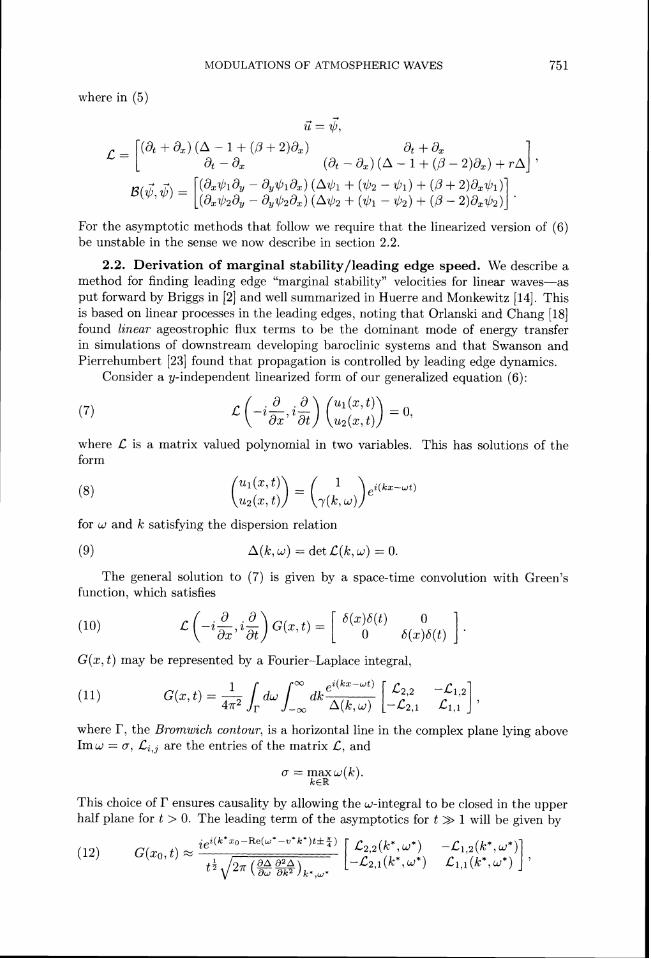
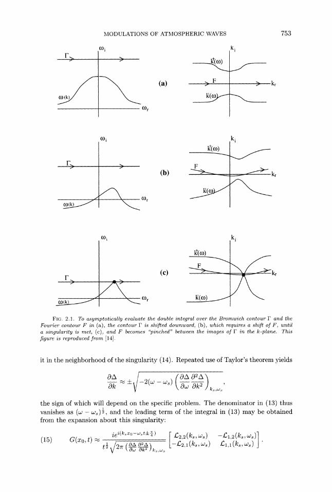
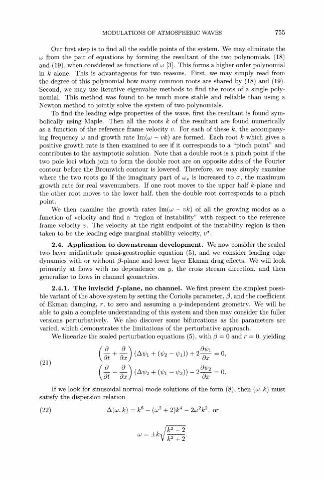
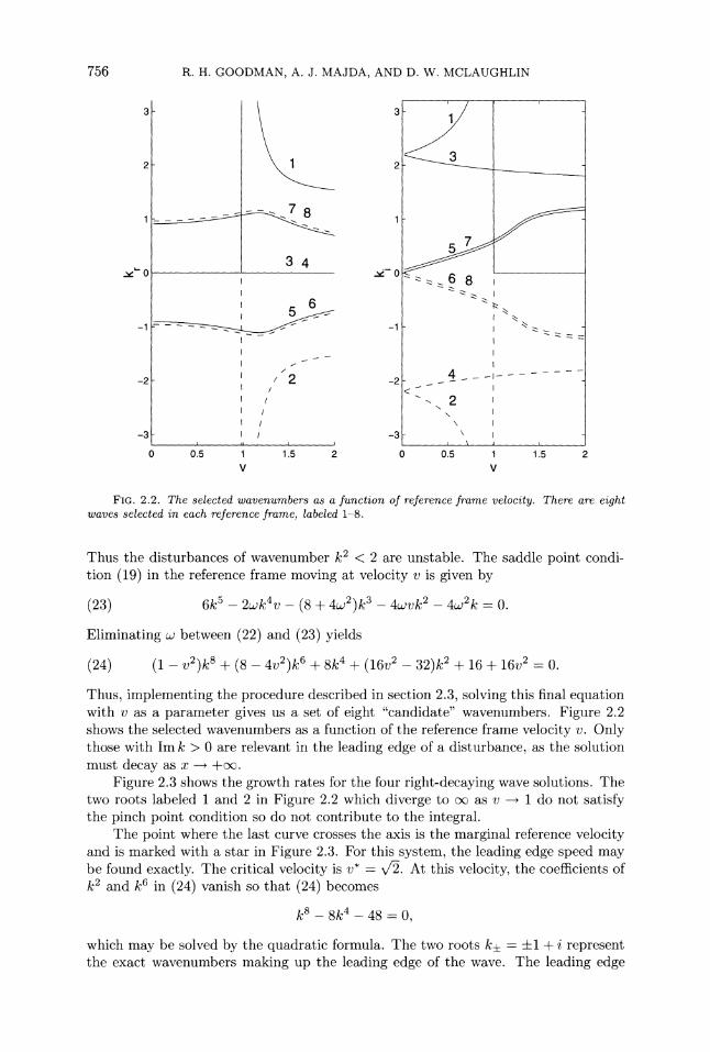
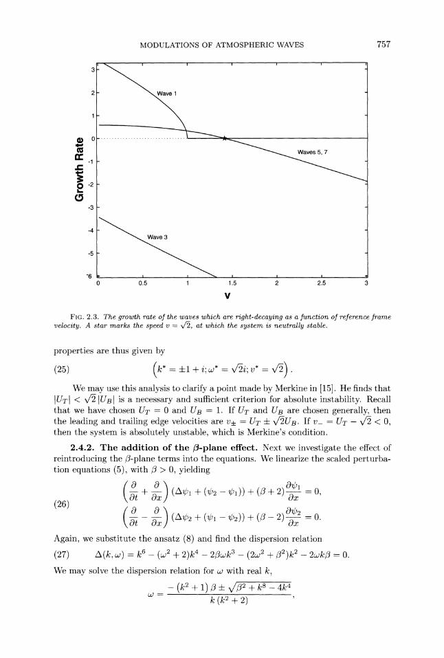
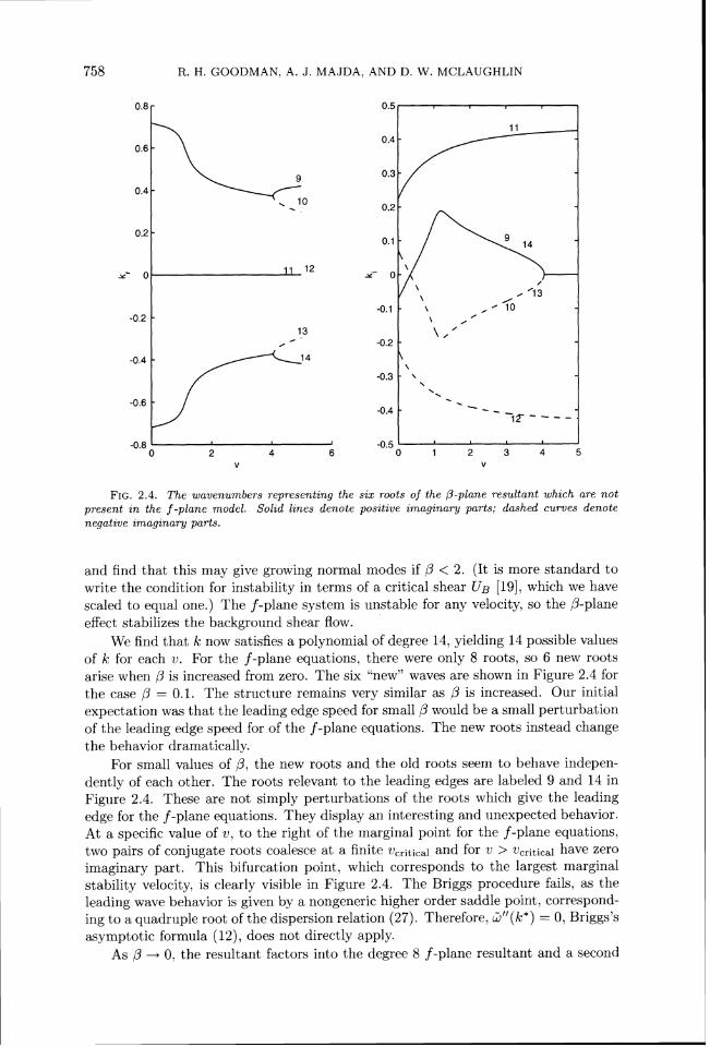
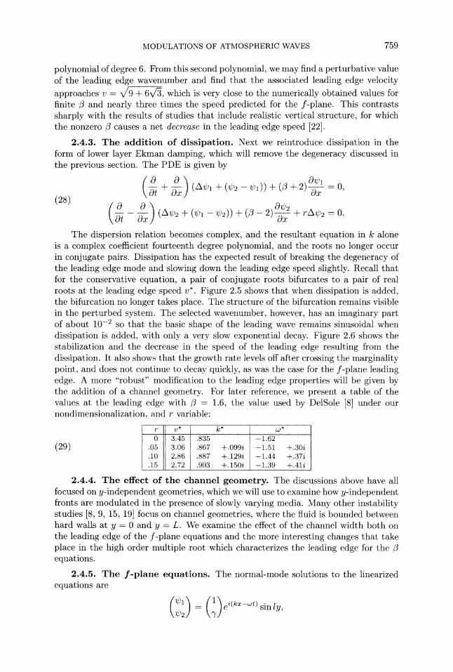
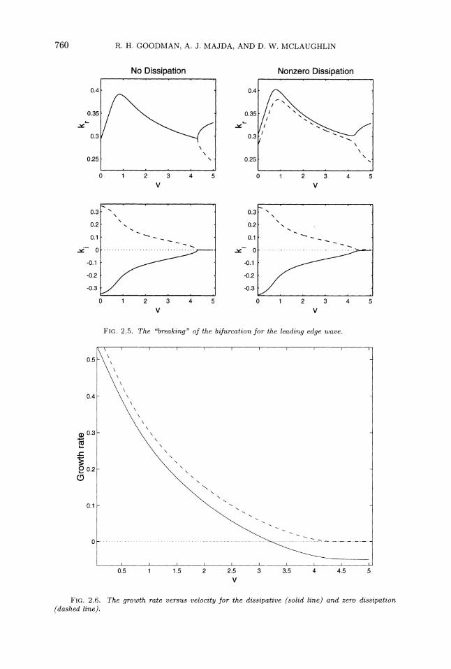
R H GOODMAN A J MAJDA AND D W MCLAUGHLIN
No Dissipation Nonzero Dissipation
04
025 025
-0 1 2 3 4 5 0 1 2 3 4 5
v v
F I G 2 5 The breaking of the bifurcatzon for the leading edge wave
FIG26 The growth rate versus velocity for the dzssipative (solid line) and zero disszpation (dashed line)
MODULATIONS OF ATMOSPHERIC L W E S 761
FIG27 Marginal stabzlzty velocity vs y-wavenumber 1 showzng good agreement between the values computed vza the perturbatzon expansion (+) and vza the numerical procedure (0)
a-here 1 = FYe shall take N = 1as this mode is the most unstable The dispersion relation is
As before the formula for selected ivavenumbers is of fourth degree in k2 A wide channel gives rise to a srnall wavenumber 1 = t which admits the pertur-
bation expansion
The perturbation series gives excellent approximations to the values of the leading edge velocity as shown in Figure 27 Slerkine [15] finds bv a formal argument that the condition for absolute instability of this system is given by UB gt f i ( 1 - $) I2 which agrees with the perturbation series to leading order
246 The P-plane equations in a channel In this section tve investigate the effect of the channel geometry on the high order root tvhich determines the leading edge wave for the 3-plane system The effect is more dramatic than of simply adding
R H GOODLIAN A J MAJDA AND D W LICLAUGHLIN
F I G 2 8 Growth rate versus veloczty wzth 1 = 1 (solzd) 1 = 25 (dashed) and 1 = 4 (dash-dot)
dissipation DelSole in [8]studies the 3-plane equations in a channel and does not shot$ a high order root a t the leading edge This leads us to studv whether the channel geometry is sufficient to remove the degeneracy
We study the 3-plane equations with 7 = 0 and find that k satisfies a polynomial equation of degree 16 We fix 3 = 16 corresponding to the value used in [8]and decrease the channel width from xwhich is equivalent to increasing 1 from zero The system goes through three stages (i) When the channel is very wide the behavior is essentiallv the same as for a channel of infinite width (ii) As the channel is nar- rowed however a second high order root forms at a velocity greater than The1 1
two quadruple roots move together as the channel is narrowed further and at some critical channel width annihilate each other (iii) Beyond this value the multiple roots disappear and the svstem contains no degeneracy In Figure 28 the growth rate is shown as a function of velocity for values of 1 in the three above regimes (i) When 1 is small the behavior is the same as when 1 = 0The leading edge wave bifurcates a t some finite value of I beyond which there is no pinch point (ii) For intermediate 1 there exist two critical velocities separating two unstable wave packets (iii) For 1 sufficiently large these two critical velocities and hence the associated wave packets merge and the leading edge wave is determined by a double root as in the standard Briggs procedure Such an 1 corresponds to a channel whose width is two to three tirnes the tvavelength in the zonal direction
This shows that the multiple root which appeared to determine the leading edge behavior is an artifact of the one-dimensional geometry However even without this degeneracy the leading edge speed is significantly enhanced in the presence of nonzero 3
763 hIODULATIONS OF AThlOSPHERIC WAVES
3 Modulation by nonlinearity and weakly variable media With the description of the marginally stable linear wave front in hand we now examine the effects that nonlinearity and weak variation in the background shear flow have on downstream developing dynamics Recall that the atmosphere is absolutely unstable off the eastern shores of continents and convectively unstable over the oceans An easy way to model this is to allow the strength of the shear to vary slowly To create a variable medium we linearize (1) about the (nearly) exact solution
This is not an exact solution to (1)but we may think of it as arising due to a balance of unwritten damping and driving terms in the equation
JVe again consider the quasi-geostrophic potential vorticity equations as given in the abstract form (6) We further assume that the solutions depend only weakly on the transverse y direction through a scaled variable Y = ay We therefore write as a generalization of (6)
where for the quasi-geostrophic equations with shear flow as given in (33)
and
To study how the leading edge wave is slowly modulated by the additional terms in this equation we develop a multiple scales expansion centered around the y- independent leading edge mode e ( ~ - - ~ )b If we assume that the solution is in- dependent of y to leading order then the only y-dependence in the solution will be generated by the variable coefficient term M
JVe follow the standard procedure in deriving envelope equations with one major exception we center our asymptotic expansion on the linear fronts described in the previous section instead of on normal modes A normal-mode expansion requires a weak instability so that the leading order term in the expansion can be approximated by a neutrally stable mode By using the linear front we are able to carry out the expansion for strongly unstable systems by working in the reference frarne moving with the front A major side effect of centering our expansion on these fronts is that nonlinear terms will not enter our envelope equations even if nonlinearity is present in the system The form of the asynlptotics will show that this method is applicable only if the variable coefficient term M satisfies certain restrictions
11-e recall that a multiple scales expansion to a PDE consists of expanding both the solution and its derixatives in powers of small parameter 6 and solving a sequence of equations at increasing powers of 6 The nlodulation equations are then derived as the result of solvability conditions for these equations necessary to preserve the assumed ordering of the expansion Ye write
764 R H GOODMAN A J hlAJDA AND D W MCLAUGHLIN
where is the linear leading front slowly modulated in space and time + q ( l ) = A(ltYT2)ge(k-t)
and the first correction is given by
where X Y and Tl are C(E) slow space and time variables T2 is an 0 ( t 2 ) slow time variable and 6 is a slow space variable in the reference frame moving with the front The terms and $(22)arise due to the nonlinearity The result of the $ ( 2 1 1 )
asymptotics derived in section 31 may be summarized as follows Asymptotic result If $(lo and $(2) are defined as above then the correctaon
t e r m B zs of the form B = O ( X T I Y ) A ( J YT 2 ) and A and O satasfy
(36a) O T ~+ VOX= m ( X Y )
T h e coef icients m and p are given below in (45) and (46)
31 The leading edge perturbation expansion In this subsection we de- rive the results in (36) LYhen the solution is sufficiently small of order E or smaller then will approximately satisfy the linearized equation Since the front decays exponentially the solution will certainly be sufficiently small for sufficiently large x
We define slow time and space scales
X = E X Y = t y T I = t t and T2 = t 2 t
and expand the derivatives accordingly
d d d d d d d -+ -+t - and -+ - + ~ - + ~ 2 -d x ax ax dt a x dTl dT2
We assume that the solution depends on y only through the slow variable Y so that
The leading order equation is taken to be a slow modulation of the leading edge wave 4
(37) d ( l )= + CCA ( X YT I T2)ez (kx-wt )g
where CCdenotes complex conjugate Recall that we may form the matrix L ( k d )
from the relation
~ ~ ~ ( k x - w t ) gL (k w) e ~ ( k x - ~ t ) g=
The vector 6 must be in its null space so we may without loss of generality set
765 hlODULATIONS OF ATMOSPHERIC WAVES
We plug in the multiple scale ansatz and separate orders to derive a formal sequence of equations of the form
where the derivatives of are evaluated at the point (k d ) We see that (39) and (40) are of the form
Thus we must solve this class of linear equations First we define a resonance as a forcing term on the right-hand side which causes the solution to grow to violate the ordering (35) for large t (The solution (I) is meaningful in the reference frame moving at the leading edge velocity so it is in this reference frame we must evaluate the asymptotic ordering) By the Fredholrn alternative a resonance will occur if is in the adjoint null space of C
Nonresonance assumptzon We make the standard assumption that C is a dis- persive operator in that d l ( k ) 0 so that if a particular wavenumber and frequency satisfy the dispersion relation A ( k d ) = 0 then in general nlultiples of the ordered pair (nk n d ) will not also satisfy the dispersion relation ie A(nk nd ) 0 In fact we will make the slightly more general assunlption that terms on the right-hand side of (41) of the form = oeklx-lt) for (k l d l ) (kd) which arise in the course of this expansion satisfy A(kl d l ) 0 SO that (41) is solvable Fortunately for all the systems we anvestagate the nontianashzng condataon
is satisfied and there is no resonance due to nonlinear terms
311 0 ( e 2 ) The leading order ansatz (37) solves the O(s) equation so we may move to the next order The O(s2) equation then becomes
where we have let d = kx - d t It will be convenient to consider the effect of the linear and nonlinear forcing terms separately
Nonlinear terms The term a(() (I)) in (42) gives rise to terms on the right- hand side proportional to e2 e c 2Irn By the above nonresonance assun~ption these will give rise to terms of the same form in the expression for $(2) In the reference frame moving with the leading edge front these have zero growth rate so are not resonant
766 R H GOODMAN A J hlAJDA AND D W LICLAUGHLIN
Linear terms Given the nonresonance assumption we need consider only the linear portion of (42)
The tern1 on the right-hand side will give rise to resonances unless it is perpendicular to the adjoint null space of C Enforcing this nornlal condition gives the general solvability condition [l11 Changing independent variables to
the amplitude A is seen to depend only on the group velocity variable E
We define for the (E r ) reference frame the wavenumber and frequency
k = k and 2 = u -vk
A (nonunique) solution is given by 2= (ao ) ~ where
and primes denote derivatives with respect to k The condition that the solution decay as x + cc prevents us from including a constant terrn in the general solution We include in our full solution an additional solution to the homogeneous equation which will be used in eliminating resonances due to the variable medium Thus the full solution reads
4
(2) = ((i)+ O(X T1IAg) + ~ 2 2 ) ~ - 2 1 m ~ e t ~ + ~ ( 2 l ) ~ 2 z 0 + cc(43)
where the terms $(211) and $ ( 2 s 2 ) are generated by the nonlinear forcing term B
312 O ( e 3 ) Again we consider the linear and nonlinear terms separately Nonlinear terms The terms on the right-hand side of the forrn B(amp() g(2))
and B((~)$()) will lead to forcing terrns that look like e(kx-wt) and e z ( ( k ~ f 3 z k ~ ) x - ( d ~ f 3 z ~ ) t )as well as terms of the type discussed in the previous section on nonlinear terms By the nonresonance assumption these terms do not contribute to resonances
We note here the effect of centering our asyrnptotics on the leading edge front If the expansion had been performed for nornlal modes then the imaginary parts of k and d would be zero and there would be a forcing term proportional to ez(kx-wt) arising due to the nonlinearity This is precisely how the cubic nonlinearity arises when the nonlinear Schrodinger or Ginzburg-Landau equation is derived as an envelope approximation-a rnechanisrn lacking in this wave front situation
Linear terms As the nonlinear terms do not in general cause resonances the solvability condition for (40) cornes entirely frorn the linear terms and the ordering of the expansion is violated unless
- det [ 1 M (-kll)]A - det [ 1 AYY= 0Cy ( -ampCI2)]
MODULATIONS O F AThlOSPHERIC WAVES
Define
m = i det [ I M A()I We may split (44) in two by taking a derivative with respect to T recalling that A = L + vampAs AT 0 the remaining terms will be aT =
m(X Y)) = 0
This may be integrated once to obtain
with constant of integration F We may solve the O equation to obtain
This explicit formula for O shows that the asymptotic ordering could be violated if m(X Y) is not subject to rather stringent restrictions In general we rnay set F to be
which means this limit must exist for each Y in the donlain considered We then use (48) to eliminate O from (44) yielding
32 The two layer f -plane without dissipation The first rnodel for which we discuss the leading edge rnodulation equations is the inviscid f-plane The nondi- rnensionalization of this model and the determination of the properties of its leading edge linear front are discussed in section 2
The leading order linear operator is discussed in section 241 Recall that the linear part of the front is of the form
where the wavenumber frequency and velocity are given by
To form the coefficients of the two main modulation equations described in (36) we need to compute the following quantities
768 R H GOODMAN A J MAJDA AND D W hlCLAUGHLIN
as well as
det [ i M (-)I and det [ I CYI ()I Substituting the leading edge quantities (52) into the preceding expressions yields
ALL= 16i
A = 8amp(l + i)
det [ i 1 M (-)I = 8(-1 + i (1 + amp))(-V1 + i ( h -
where the coefficients are given in the following table for
Thus the final equations are given by
0 + ampOx = iampVB + (1 - i)VT
where VT and VB are the barotropic and baroclinic parts of the velocity respectively as defined in (2)
33 -plane equation with Ekman drag We are unable to perform this asymptotic expansion for the Bplane equations when I- = 0 due to the high order real root at the leading edge We can however derive amplitude equations when dissipation is included Using the values given in (29) we derive equations of the form
= 16 with r as given in the table
Note the interesting fact that as the dissipation increases in the full equation the diffusion actually decreases in the Y direction as it is enhanced in the 6 direction
4 Numerical experiments Next we confirm numerically the asymptotic pro- cedure described above That the wave moves at the selected speed and has the correct decay properties has been computed by others [7 211 The leading edge speed wavenumber and frequency have been well verified for systems such as we are studying but the challenge in confirming the asymptotics is in resolving the exponen- tially decaying leading edge over several orders of magnitude In addition the slow time scales and long spatial scales imposed by the asymptotic problem require that the numerics be carried out on a large domain for long times While second order methods would certainly be sufficient to verify the basic properties of the unmodu- lated system accurate representation of the modulations due to the weakly varying coefficients over a long domain requires a higher order method
769 hIODULATIONS OF AThIOSPHERIC WAVES
41 Description of numerical experiments To write a code that would implement the atmospheric wave equations to the accuracy needed would be an ex- tremely difficult task so we choose to validate the asymptotics on a simpler model problem-a variable coefficient complex Ginzburg-Landau equation
This equation is often used as a model for the evolution of systems with weak nonlinearities and weak instability [17] and has been derived as a model for the two layer quasi-geostrophic equations by Esler [9] The problem we solve is to set u= 1 at x = 0 with conlpactly supported initial conditions allowing a wave propagate to the right
Although our general derivation of modulation equations was performed for vector systems a similar derivation may be done for this scalar equation For later reference the selected wavenumber frequency and velocity are
42 Numerical difficulties In order to get meaningful results from this nu- merical experiment a code of higher-than-usual accuracy will be needed especially for the spatial discretization To see why recall that the important terms are A and 0where the full solution in the leading edge is of the form
where k and UJ are complex In order to compare theory with the numerical experi- ment we must know A to several decimal places but over the domain of computation u decays from order one down to ~ ( e - ~ ) If standard Fourier methods are used to compute the derivative then the solution can only be resolved down to size 10-l6 in double precision arithmetic We instead use high order methods which are more local in nature which are able to resolve the amplitude of a decaying exponential over greater distances [12]
For temporal discretization there are two competing difficulties which lead us to our numerical method First we have stiffness due to diffusive and dispersive terms in our PDE which would suggest that we use an implicit method Second we have nonlinear terms and we would like to avoid using implicit methods and needing to solve fully nonlinear equations at each step We would also like to be able to use a high order method so as not to squander the accuracy of the spatial discretization
43 Summary of method Briefly our method will consist of a method of lines First we impose a spatial discretization and specify a method of computing approximate spatial derivatives This reduces the PDE to a system of ODES for the vector 6(t)which is then solved by a suitable time stepping method
44 Spatial discretization The spatial discretization is performed by a mul- tidomain Chebyshev collocation due to Yang and Shizgal [24] Generally Chebyshev methods are much more adaptable to boundary conditions than are related Fourier methods lye begin by defining the standard Chebyshev collocation method and then explain the multidonlain version On the interval [-I 11 we define the Gauss- Lobatto-Chebyshev (GLC) points
770 R H GOODhIAN A J LlAJDA AND D Mr LICLAUGHLIN
Let f be a smooth function defined on [-I 11 and let f b e the vector f k = f (xk) of values at the GLC points Then we may compute an approxinlate derivative as
f 1 ( ~ k )= Dfkgt
where [4]
where c = 1 for 0 lt j lt N and co = cAi= 2 and x are as defined in (55) (This comes from representing f as a sum of the first n + 1 Chebyshev polynomials and such a derivative converges faster than any power of N as N + m)
It is not practical to implement this method over a large computational domain as D is a dense matrix and becomes extremely ill conditioned for large values of n Therefore we consider a piecewise method using overlapping subdomains as described by Yang and Shizgal in [24] In this method we partition the interval into overlapping subdomains of equal length so that the last two GLC points in one subdomain coincide with the first two points in the next subdomain If we choose to partition an interval of length L into J subintervals and want to use approximating polynomials of degree N then there will be
total collocation points and the length lSub of the subintervals will be given by
2L lsub = (J f 1) + ( J - l ) c o s
Such a partitioning is shown in Figure 41
The kth subdomain
X0 fi + x x
N-I N 2N-I
F I G 41 Partitioning of a n znterval znto J ouerlappzng subdomazns Ik
If we let D be the ( N + 1) x ( N + 1) collocation derivative operator for a single subdomain with the points in the subdomain labeled 0 through 1Y then the full operator 2) has a nearly block diagonal structure The resulting linear system is nearly block diagonal We may then use this approximate derivative to discretize a boundary value problem which is very efficiently solved by Gaussian elimination using a specially adapted partial pivoting scheme subject to the constraint that two rows may be interchanged only if they are in the same block Such a matrix may
h1
hIODULA4TIONS OF AThlOSPHERIC WAVES
FIG42 T h e vanable coeficzent p used zn one expenment
be factored in O(JN3) steps and the forward and backward substitutions may be performed in O ( J N 2 ) steps The elements of the matrix may be stored in a one- dimensional array consecutively by rows with all the arithmetic done in place with zero fill-in Thus with N fixed quite large systems may be solved very efficiently In practice lZr = 6 was found to be sufficient
45 Time stepping To solve this ODE the right-hand side is split into two pieces one containing all the terms responsible for stiffness and for instability and one containing all the convective and nonlinear terms The ODE may then be written in the form
and solved by a high order splitting algorithm described below The time stepping is done using the implicit-explicit multistep schemes due to
Ascher Ruuth and Wetton [I] These allow us to compute the nonstiff cubically nonlinear terms and advection terms explicitly needing only to solve implicitly for the terms due to the higher order spatial derivatives This may be thought of as a high order splitting method which allows us to avoid costly iterations of a nonlinear solver
46 Results of one-dimensional simulations Recall that the one-dimensional numerical experiments are performed for the model equation
For all experiments reported the parameters used were zt = 3 P = 1 and y = 2 which makes the equation convectively unstable The experiments were performed with sixth order piecewise collocation and a total of 1000 subdomains for 0 5 x 5 1000 A variety of variable coefficient functions p(tx) were used an example of which is plotted in Figure 42 with E = 2This function was generated by a random Fourier sine series Other functions we used for p included Gaussians sinusoids and sums of randomly placed Gaussians The quality of the results was fairly independent of the shape of the variable coefficient as long as the criterion was met that the mean of p was zero
Figure 33 shows a contour plot of the wave spreading to the right at constant velocity vwith the variable coefficient as shown in Figure 32
To postprocess these numerical results in the parallelogram region pictured in Figure 43 we form A(1+ EO) by dividing the full solution by ez(kx - t ) Th is region is defined by to lt t lt t l and xo - vto lt x - vt lt XI - zftl In this region the solution has an amplitude of about ul = 15 at the left edge and about (uJ= 10-l6 at the right edge due to the exponential decay of e Thus we remove this large variation and focus on A( l + euro0)
R H GOODhIAN A J LIAJDA AND D W LICLAUGHLIN
real (u)
F I G 4 3 Solutzon to the PDE spreadzng to the rzght The parallelogram regzon shous the regzon zn ( [ T 2 )varzables where the slowly Laryzng functzons A and O are defined
Next
is formed from p where recall TI = et lt = t ( z - z i t ) This allows A to be calculated from the solution to the full PDE Il-e rnay then cornpare its evolution with that of the envelope equation The initial and boundary values of A are used to nurnerically conlpute the evolution of A under the reduced equation (51) and the results are compared with the values of A obtained frorn the full sirnulation Results are shown in Figure 33 The relative error between the envelope A as cornputed from the full solution and from the asynlptotic reduction is shown in Figure 45 Each line in the contour plot represents a one percent increment in the relative error with a rnaxinlal relative error of about seven percent The relative error is clearly largest at the left of the moving interval where the solution to the PDE is largest and nonlinear effects are rnost important
To show the asynlptotic validity in a rnore quantitative manner we run the sim- ulation for two different values of t and show that the error norrn for A decreases by o(t) with p = s inX Formally the order of the asymptotic expansion is O(t3) In the case of scalar equatmns ((2) the O(e2) term in the asymptotic expansion ( 3 5 ) vanishes so that
773 hfODULATIONS OF ATMOSPHERIC WAVES
FIG44 T h e amplitude A computed from the full simulation (solid) and vza the reduced equatzon (dotted) T h e contour znterval for each is l
Therefore
The error in the computed value of A at large time t = 135 is plotted in Figure 46 Error(euro=a )
The empirical convergence rate given by log Erro t ( r=QI is 165 While not quite
O(E) it is at least o(E)
It would be useful to see if the error estimate improves as E is further decreased but it is difficult to run the numerical procedure with E much smaller than because we must run the code for times of O(E-) on intervals of length O(E-) in order to compare our theory with the numerics As the order is only exact in the limit as E 0we may only be able to verify O(E) convergence
In section 31 we showed that the inhomogeneitl- must additionally satisfy a finite mean condition (50) We now investigate the importance of this numerically To show that the asymptotic expansion breaks down when ydX grows large we now show an example where the order of the method begins to break down We choose y(x) to be a smoothed step function of height e2 and width 4016 and we allow the wave to propagate until it is about eighty percent of the way through the interval We then compute the value of A bl- the above procedure and compare the errors when E = with those when E = i The difference between the two computed values of A is
R H GOODMAN A J MAJDA AND D W MCLAUGHLIN
F I G 45 T h e relative error in A computed v ia t w o methods Con tour znterval 01m a x i m u m relative ewor 07 near left edge
F I G 4 6 T h e dzfference an the ampli tude A computed numerzcally and via the envelope equatzon for t = (solid) and t = $ (dashed) for inhomogenei ty p = sin(X)
shown in Figure 47 We compute the empirical convergence order a t the final time which is approximately 107 so that the convergence is approximately first order which is a significant drop off from the previous case This shows that the mean zero condition on the variable coefficient term (p for complex Ginzburg-Landau M for a general vector system) affects the convergence of the method and is not merely a formal breakdown in the ordering
FIG47 As zn (-16)uith shelf-like z~nnnble coejicient
5 Conclusion Ye have investigated a mechanism which may be respo~isible for downstream development in midlatitude storm tracks We have identified linear processes in the leading edge of developing storm tracks as a possible mecha~iisni for dowrlstream development and applied the predictiorls of this theory to a two layer system of quasi-geostrophic equations which is known to exhibit downstrearii development
In investigating the leading edges of unstable baroclinic waves we have made several observations most notably we find that the leading edge speed changes dis- continuously as the parameter 3 is increased from zero due to a change in the algebraic structure of the equations which determine the roots Another interesting feature a e have explored 1s the degenerate root in the leading edge mode of the 3-plane equa- tions and how this is regularized both by dissipation and more interestingl by the constraints of a finite-width channel Studies show that in models including realis- tic vertical structure the leading edge speed is actually reduced by the 3-effect li have also clarified some points made by Slerkine [15] about the absolute instability of constant shear flow sollitions of the two laler f-plane problem
NTe then investigated the interaction of leading edge modes with a weakly varying medium iVe generalized the standard [17] multiple scale procedure for wave pack- ets centered on unstable normal rriodes to the case of wave packets centered or1 thr wavenumber at the leading edge front Under the scaling ansatz studied the prc- dominant effects are captured by linear modulation equations and are applicable onlt ahead of a moving front where the solution and the nonlinear correction terms art quite small This method was applied to derive modulation equations for the leading edges of baroclirlic disturbances interacting with variable mean flows The validity of this asymptotic represerltatiorl wai verified ~iumerically on a model system of equa- tions and agreement was found ahead of the front though only in regions where the solutioli is very small Clearly 111 order for the asymptotic representatloll of the lead- ing edge to be useful one must connect this leading edge behavior with that slight11 behind the leading e d g ~ nhere rioliliriear effects become important
Acknowledgment R H Goodman wishes to thank Lucent Techliologies-Bell Laboratories where he was an NSF University-Industry postdoctoral fellow while thii paper was being conipl~ted
776 R H GOODLIAN A J LIAJDA AND D W LICLAUGHLIN
REFERENCES
[I] uhI ASCHER S J RUUTHAND B T R I-ETTON Implzczt-expliczt me thods for t ime-dependent partial dzfferentzal equatzons SIAhI J Numer Anal 32 (1995) pp 797-823
[2] R BRIGGS Electron S t ream Interact ion w i th Plasmas MIT Press Cambridge MA 1964 [3] W S BURNSIDE T h e Theory of Equat ions 8th ed Hodges Figgis and A N D A I- PANTON
Co Dublin 1924 [4] C CAYUTO Ll Y HUSSAINI A QUARTERONI T A ZANG Spectral Methods i n Fluzd AND
Dynamzcs Springer-Verlag New York 1988 [5] E K CHANGAND O n the dynamzcs of a s t o r m track J Atmospheric Sci 50 I ORLANSKI
(1993) pp 999-1015 [6] E K LI CHANG Downstream development of baroclznzc waves as znferred f rom regresszon
analyszs J Atmospheric Sci 50 (1993) pp 2038-2053 [7] G DEE A N D J LANGER Propagating pat tern selectzon Phys Rev Lett 50 (1983) pp 383-386 [8] T DELSOLEAbsolute instability induced by disszpatzon J Atmospheric Sci 54 (1997) pp
2586-2595 [9] J G ESLER W a v e packets zn szmple equilibrated baroclinic sys tems J Atmospheric Sci 54
(1997) pp 2820-2849 [lo] B F FARRELL Pulse asymptot ics of t he C h a n ~ e y baroclznzc instabzlzty problem J Atmospheric
Sci 39 (1982) pp 507-517 [ll] J D GIBBON A N D 11 J LICGUINNESS Amplztude equatzons at t he crztical poznts of unstable
dispersive physzcal sys tems Proc Roy Soc London Ser A 377 (1981) pp 185-219 [12] R H G O O D ~ I A N Asympto t i c s for the Leading Edges of Mzdlatztude S t o r m Tracks PhD thesis
New York University New York 1999 [13] I M HELDA N D S LEE Baroclinzc wave-packets zn models and observatzons J Atmospheric
Sci 50 (1993) pp 1413-1428 [14] P HUERRE A N D P A ~ ~ O N K E U I T Z Local and global znstabzlzties zn spatially developzng flows
in Ann Rev Fluid LIech 22 Annual Reviews Palo Alto CA 1990 pp 473-537 [15] L L~ERKINEConvect ive and absolute instability of baroclznzc eddies Geophys Astrophys Fluid
Dynam 9 (1977) pp 129-157 [16] L ~ I E R K I N EAND LI SHAFRANEK localizedT h e spatial and temporal evolut ion of unstable
baroclinic dzsturbances Geophys Astrophys Fluid Dynam 16 (1980) pp 175-206 [17] A C NELYELL Envelope equations in Nonlinear Wave klotion (Proceedings of the AhIS-SIALl
Summer Sem Clarkson Coll Tech Potsdam NY 1972) Lectures in Appl hlath 15 AhIS Providence RI 1974 pp 157-163
[18] I ORLANSKI E K hI CHANG Ageostrophic geopotential fluxes i n downstream and up- AND s tream development of baroclznic waves J Atmospheric Sci 50 (1993) pp 212-225
[19] J PEDLOSKYFznzte-amplitude baroclznic wave packets J Atmospheric Sci 29 (1972) pp 680-686
[20] J PEDLOSKYGeophysical Fluzd Dynamics 2nd ed Springer-Verlag New York 1987 [21] J A POLYELL A C NEWELL A N D C K R T JONESCompe t i t ion between generzc and
nongenerzc fronts zn envelope equatzons Phys Rev A (3) 44 (1991) pp 3636-3652 [22] A J ~Ihlhl0NS A N D B J HOSKINS T h e downstream and upstream development of unstable
baroclinzc waves J Atmospheric Sci 36 (1979) pp 1239-1254 [23] K L SWANSON Nonlinear wave packet evolution o n a baroclznically AND R T PIERREHU~IBERT
unstable jet J Atmospheric Sci 51 (1994) pp 384-396 [24] H H YANG A N D B SHIZGAL Chebyshev pseudospectral mu l t i -domain technzque for viscous
floul calculation Comput Llethods Appl LIech Engrg 118 (1994) pp 47-61
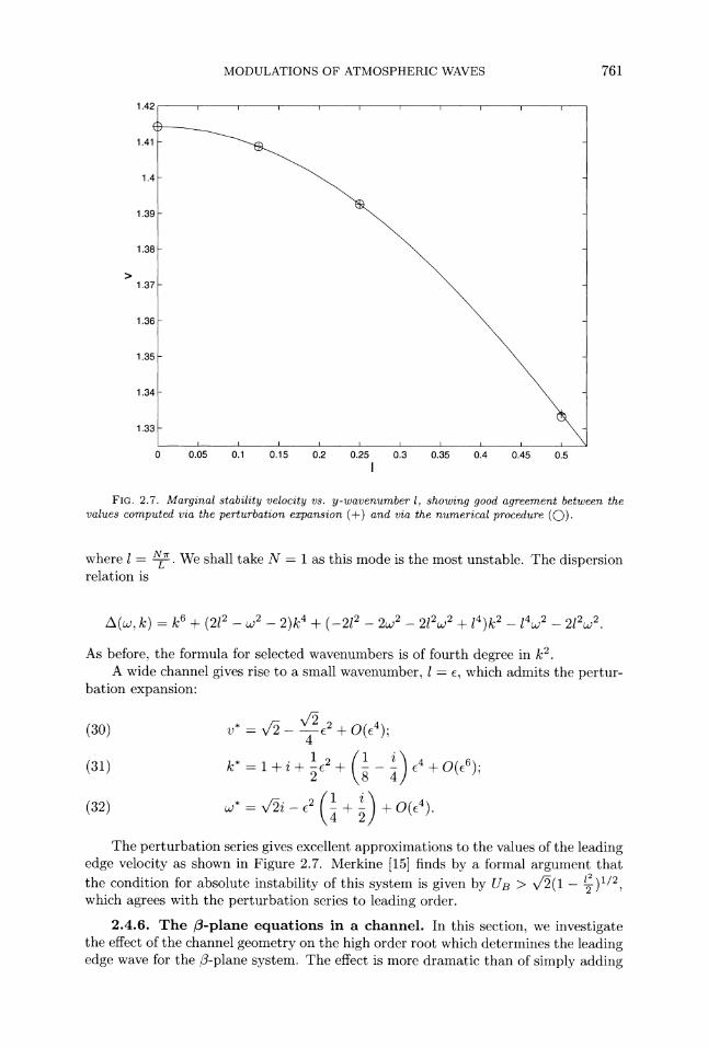
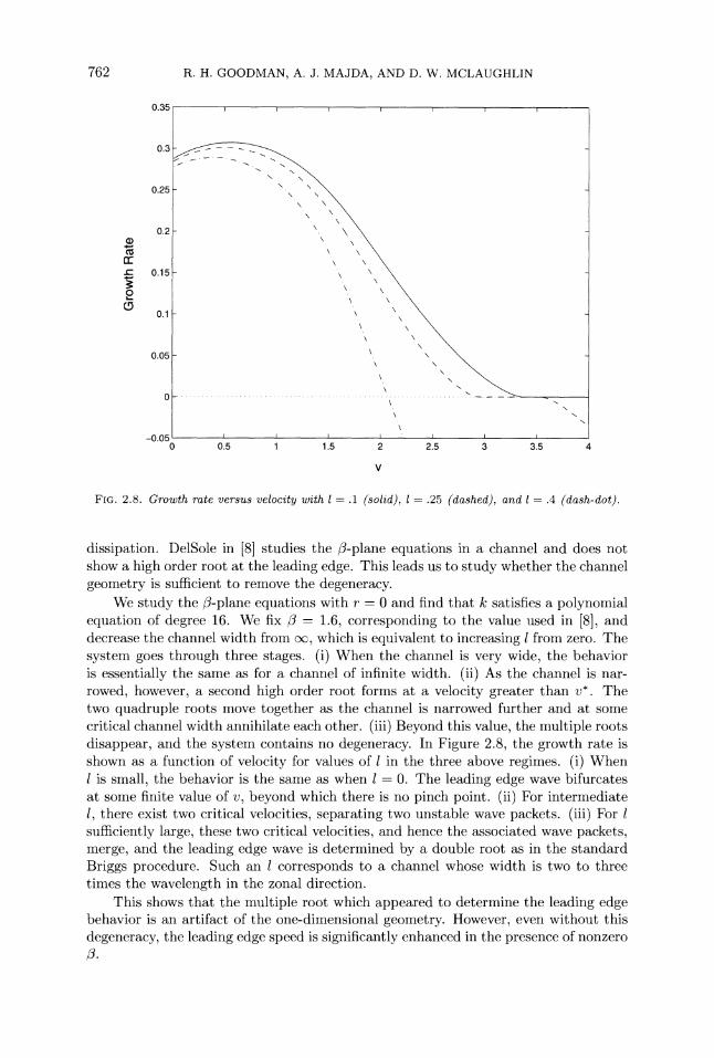
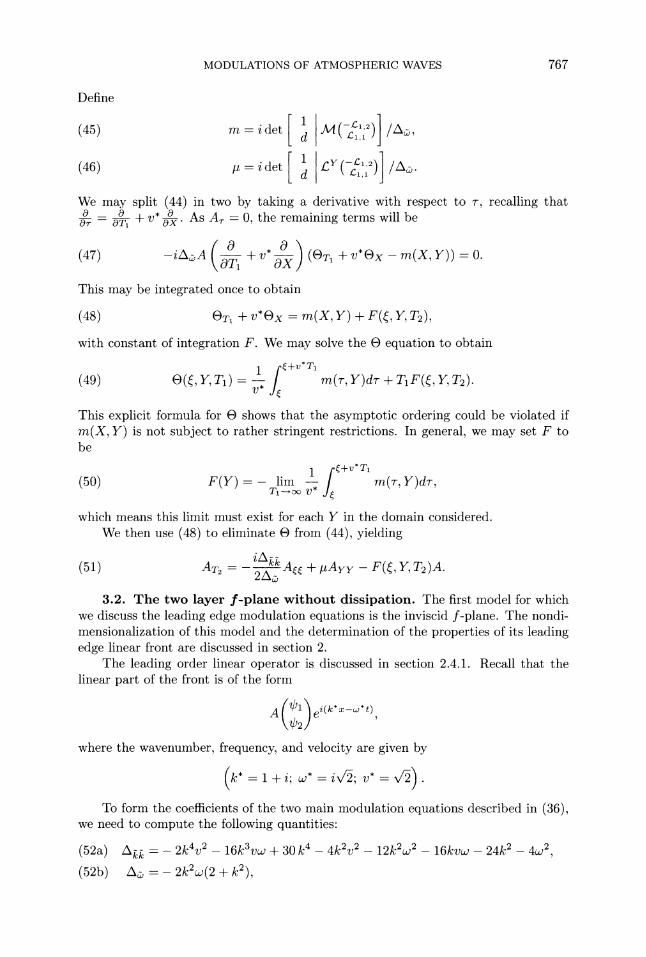
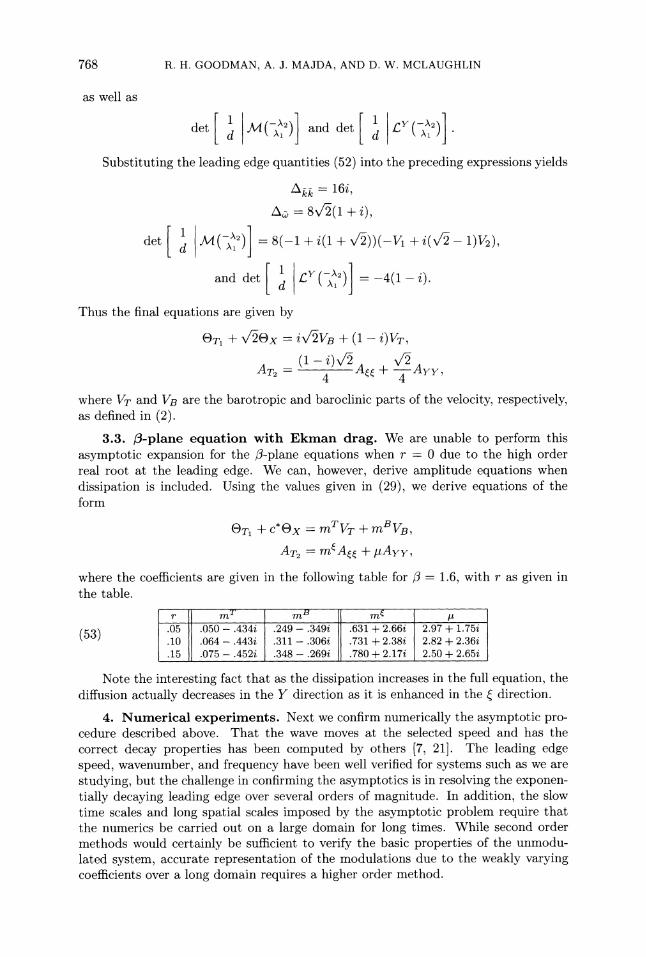
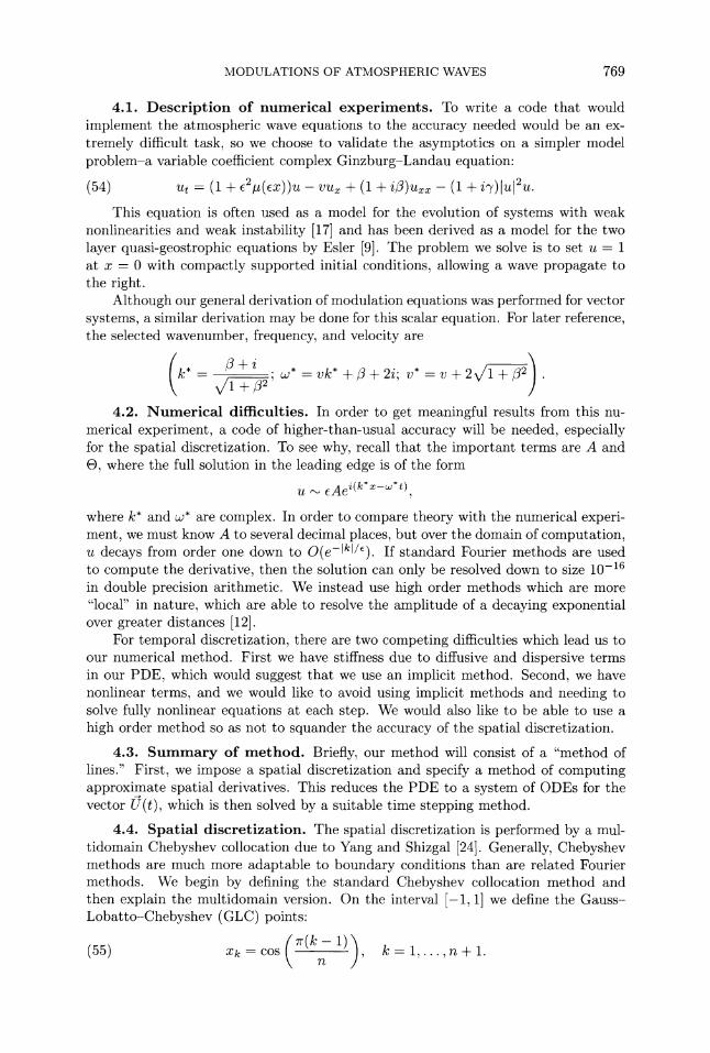
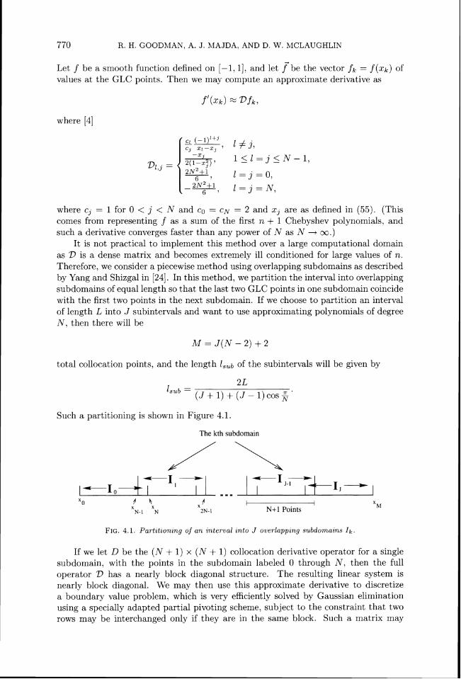
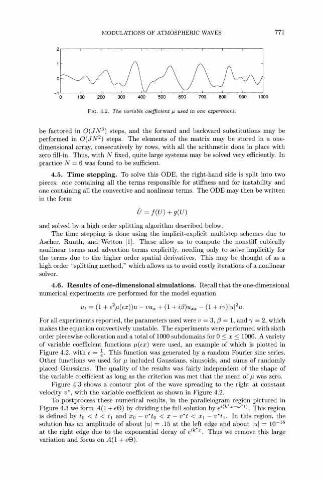
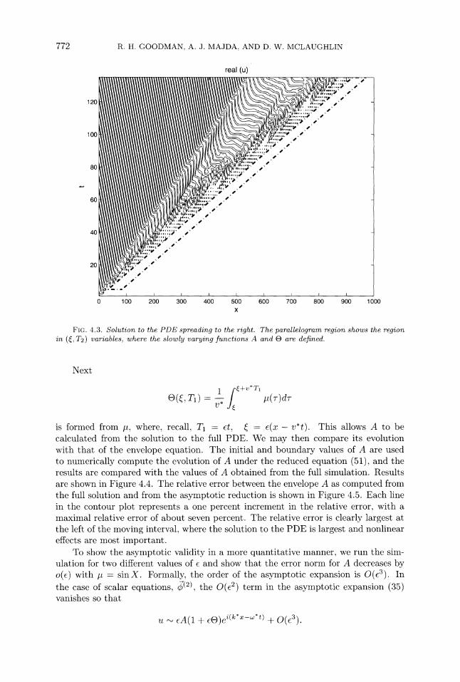
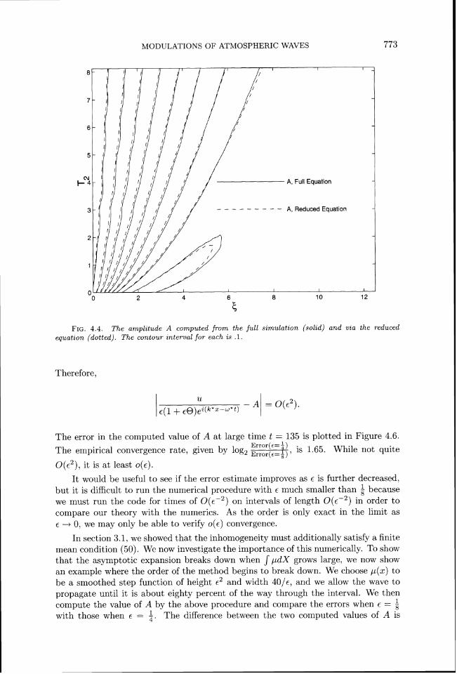
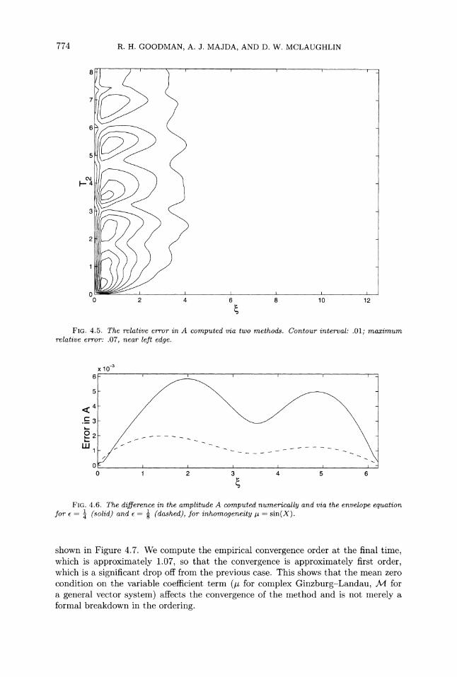
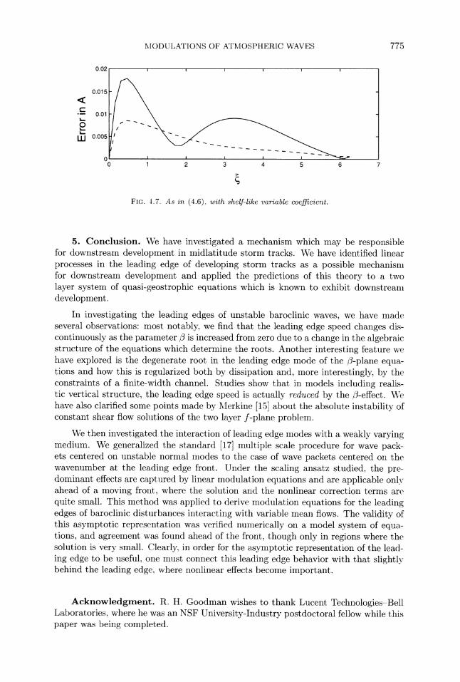

![Modulations Cover Score · modulations for percussion trio Full Score [2017] Christopher LaRosa Perusal](https://img.pdfslide.us/doc/110x75/5e88d76cc25a3d277f3b6748/modulations-cover-modulations-for-percussion-trio-full-score-2017-christopher.jpg)