Biogeosciences, 8, 841–850, 2011www.biogeosciences.net/8/841/2011/doi:10.5194/bg-8-841-2011© Author(s) 2011. CC Attribution 3.0 License.

Biogeosciences

MODIS observed phytoplankton dynamics in the Taiwan Strait:an absorption-based analysis

S. Shang1, Q. Dong1,2, Z. Lee2, Y. Li 1, Y. Xie1, and M. Behrenfeld3

1State Key Laboratory of Marine Environmental Science, Xiamen University, Xiamen 361005, Fujian, China2Geosystems Research Institute, Mississippi State University, MS 39529, USA3Department of Botany and Plant Pathology, Oregon State University, OR 97333, USA

Received: 25 September 2010 – Published in Biogeosciences Discuss.: 27 October 2010Revised: 20 March 2011 – Accepted: 29 March 2011 – Published: 6 April 2011

Abstract. This study used MODIS observed phytoplanktonabsorption coefficient at 443 nm (Aph) as a preferable indexto characterize phytoplankton variability in optically com-plex waters. Aph derived from remote sensing reflectance(Rrs, both in situ and MODIS measured) with the Quasi-Analytical Algorithm (QAA) were evaluated by comparingthem with match-up in situ measurements, collected in bothoceanic and nearshore waters in the Taiwan Strait (TWS). Forthe data with matching spatial and temporal window, it wasfound that the average percentage error (ε) between MODISderived Aph and field measured Aph was 33.8% (N = 30,Aph ranges from 0.012 to 0.537 m−1), with a root meansquare error in log space (RMSElog) of 0.226. By compari-son,ε was 28.0% (N = 88, RMSElog = 0.150) between Aphderived from ship-borneRrs and Aph measured from watersamples. However, values ofε as large as 135.6% (N = 30,RMSE log = 0.383) were found between MODIS derivedchlorophyll-a (Chl, OC3M algorithm) and field measuredChl. Based on these evaluation results, we applied QAA toMODIS Rrs data in the period of 2003–2009 to derive clima-tological monthly mean Aph for the TWS. Three distinct fea-tures of phytoplankton dynamics were identified. First, Aphis low and the least variable in the Penghu Channel, wherethe South China Sea water enters the TWS. This region main-tains slightly higher values in winter (∼17% higher than thatin the other seasons) due to surface nutrient entrainment un-der winter wind-driven vertical mixing. Second, Aph is highand varies the most in the mainland nearshore water, withvalues peaking in summer (June–August) when river plumesand coastal upwelling enhance surface nutrient loads. Inter-annual variation of bloom intensity in Hanjiang River estu-

Correspondence to:S. Shang(slshang@gmail.com)

ary in June is highly correlated with alongshore wind stressanomalies, as observed by QuikSCAT. The year of minimumand maximum bloom intensity is in the midst of an El Ninoand a La Nina event, respectively. Third, a high Aph patchappears between April and September in the middle of thesouthern TWS, corresponding to high thermal frontal proba-bilities, as observed by MODIS. Our results support the useof satellite derived Aph for time series analyses of phyto-plankton dynamics in coastal ocean regions, whereas satel-lite Chl products derived empirically using spectral ratio ofRrs suffer from artifacts associated with non-biotic opticallyactive materials.

1 Introduction

While the concentration of phytoplankton pigments in thesurface ocean reflect both variability in phytoplankton stand-ing stocks and physiological state (e.g. Behrenfeld et al.,2005; Westberry et al., 2008), it has a clear impact onthe optical properties of the water, allowing its relativelystraight-forward retrieval from remote sensing measurements(e.g. Sathyendranath et al., 1994). The most common pig-ment product retrieved from ocean color remote sensing ischlorophyll-a concentration (Chl, mg m−3; frequently usedsymbols throughout the manuscript are summarized in Ta-ble 1). However, because of the optical complexity innearshore waters (Carder et al., 1989; Zhang et al., 2006) andthe simple spectral ratio approach (O’Reilly et al., 2000) usedfor the derivation of Chl, Chl product can be problematic inoptically complex nearshore waters. Alternatively, analyticalapproaches (IOCCG, 2006) based on the radiative transfertheory have been developed to retrieve the spectral absorp-tion coefficient of phytoplankton (aph, m−1). Using phy-toplankton absorption, instead of Chl, as a superior metric

Published by Copernicus Publications on behalf of the European Geosciences Union.

842 S. Shang et al.: MODIS observed phytoplankton dynamics in the Taiwan Strait

Table 1. Symbols, abbreviations and description.

Symbol Description Unit

ABI Areal Bloom Index m−1

aph Absorption coefficient of phytoplank-ton;aph(412) meansaph at 412 nm;aph(443) meansaph at 443 nm

m−1

Aph aph(443) m−1

at-w Total absorption without pure watercontribution;at-w(443) meansat-wat 443 nm

m−1

Chl Chlorophyll-a concentration mg m−3

MEI Multivariate ENSO IndexQAA Quasi-analytical Algorithm

(Lee et al., 2002)RMSE Root mean square errorRrs Remote sensing reflectance sr−1

TWS Taiwan Strait

of phytoplankton pigmentation is becoming increasingly ac-cepted (e.g. Cullen, 1982; Marra et al., 2007), especiallyfrom the remote sensing point of view (Lee et al., 1996; Hi-rawake et al., 2011). This is because the direct controllerof ocean color is the spectral absorption and scattering prop-erties of the water media (e.g. Gordon et al., 1988) ratherthan pigment concentrations, although the variations of thelatter will change pigment absorption in a non-stable fashion(e.g. Bricaud et al., 1998; Stuart et al., 1998). However, fewstudies based on in situ measurements exist to test whetheraph can be derived from satellite ocean color data with lessuncertainty than Chl. Such evidence is vital in order to con-firm thataph can function as the preferable index for charac-terizing phytoplankton variability in the upper ocean. Herewe provide results conducted over the Taiwan Strait (TWS), ashallow shelf channel that connects the South China Sea withthe East China Sea (see Fig. 1), to demonstrate that (1) phy-toplankton absorption can be retrieved more accurately thanchlorophyll-a in this optically complex ocean region fromsatellite observed ocean color and (2) changes of phytoplank-ton absorption capture phytoplankton dynamics in a vibrantand changing environment.

The TWS has complex hydrographic conditions deter-mined by the relative influence of the South China Sea WarmCurrent (SCSWC) and the Kuroshio Branch Water (KBW),which are warm, saline, and oligotrophic, and the Zhe-MinCoastal Water (ZMCW), which is cold, fresh, and eutrophic,and varies seasonally in response to changes in the mon-soonal wind (e.g. Jan et al., 2002). Several medium-sizedrivers (e.g. Hanjiang and Jiulongjiang Rivers) are located onthe western coast (mainland China) of the strait. Also alongthis coast, upwelling develops in summer, driven by the pre-vailing southwest monsoon which runs parallel to the coast

116o E 118o E 120o E 12 o E221o N

23o N

25o N

27o N

ChinaMainland

Taiwan

South China Sea

East China SeaMinjiangRiver

HanjiangRiver

JiulongjiangRiver

Taiwan Bank

DongshanIsland

Zhangyun Ridge

Penghu Islands

PenghuChannel

KBWSCSWC

ZMCW

534 535

536

537

538

539

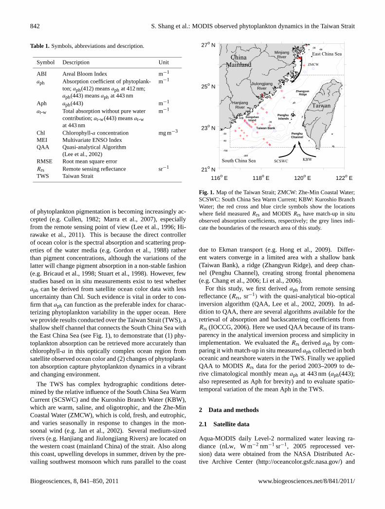
Fig. 1 Map of the Taiwan Strait; ZMCW: Zhe-Min Coastal Water; SCSWC: South China Sea

Warm Current; KBW: Kuroshio Branch Water; the red cross and blue circle symbols show the

locations where field measured Rrs and MODIS Rrs have match-up in situ observed absorption

coefficients, respectively; the grey lines indicate the boundaries of the research area of this study.

23

Fig. 1. Map of the Taiwan Strait; ZMCW: Zhe-Min Coastal Water;SCSWC: South China Sea Warm Current; KBW: Kuroshio BranchWater; the red cross and blue circle symbols show the locationswhere field measuredRrs and MODISRrs have match-up in situobserved absorption coefficients, respectively; the grey lines indi-cate the boundaries of the research area of this study.

due to Ekman transport (e.g. Hong et al., 2009). Differ-ent waters converge in a limited area with a shallow bank(Taiwan Bank), a ridge (Zhangyun Ridge), and deep chan-nel (Penghu Channel), creating strong frontal phenomena(e.g. Chang et al., 2006; Li et al., 2006).

For this study, we first derivedaph from remote sensingreflectance (Rrs, sr−1) with the quasi-analytical bio-opticalinversion algorithm (QAA, Lee et al., 2002, 2009). In ad-dition to QAA, there are several algorithms available for theretrieval of absorption and backscattering coefficients fromRrs (IOCCG, 2006). Here we used QAA because of its trans-parency in the analytical inversion process and simplicity inimplementation. We evaluated theRrs derivedaph by com-paring it with match-up in situ measuredaph collected in bothoceanic and nearshore waters in the TWS. Finally we appliedQAA to MODIS Rrs data for the period 2003–2009 to de-rive climatological monthly meanaph at 443 nm (aph(443);also represented as Aph for brevity) and to evaluate spatio-temporal variation of the mean Aph in the TWS.

2 Data and methods

2.1 Satellite data

Aqua-MODIS daily Level-2 normalized water leaving ra-diance (nLw, W m−2 nm−1 sr−1, 2005 reprocessed ver-sion) data were obtained from the NASA Distributed Ac-tive Archive Center (http://oceancolor.gsfc.nasa.gov/) and

Biogeosciences, 8, 841–850, 2011 www.biogeosciences.net/8/841/2011/

S. Shang et al.: MODIS observed phytoplankton dynamics in the Taiwan Strait 843

were subsequently converted toRrs via the ratio of nLwto extra-terrestrial solar irradiance,F0 (W m−2 nm−1) (Gor-don, 2005; also seehttp://oceancolor.gsfc.nasa.gov/DOCS/RSRtables.html). Aqua-MODIS Level-2 Chl daily data dur-ing 2003–2009, which were derived by using the OC3M em-pirical algorithm (O’Reilly et al., 2000), were also obtainedfrom the same source. These data were further processedinto Level-3 products by using Mercator projection, whichwas implemented on SeaDAS (http://seadas.gsfc.nasa.gov/doc/tutorial/sdstut2.html). The spatial resolution of thesedata was 1 km by 1 km.

Daily wind field data were obtained from QuikScatterom-eter (QuikSCAT) observations from 2003 to 2009 (http://podaac.jpl.nasa.gov), with a spatial resolution of 0.25◦ by0.25◦ (equivalent to∼25 km by∼25 km). Daily wind stress(T , N m−2) was calculated from (Stewart, 2008):

T = ρaCDU210 (1)

whereρa = 1.3 kg m−3 was the density of air,U10 (m s−1)was wind speed at 10 m above the sea surface (the QuiS-CAT measurement), andCD was the drag coefficient.CDwas calculated from Yelland and Taylor (1996) and Yellandet al. (1998). Wind stress vectors were further decomposedinto alongshore (southwesterly) and cross-shore (northwest-erly) components by applying a simple vector manipulation.

Aqua-MODIS sea surface temperature (SST,◦C) monthlymean data (4 km by 4 km resolution) during 2003–2009 weredownloaded fromhttp://oceandata.sci.gsfc.nasa.gov/. Basedon this SST data, we derived a thermal frontal probabilitymap for the TWS by following Wang et al. (2001). Briefly,we calculated the SST gradients in eight directions for eachclear pixel and chose the average over the three absolutemaxima as the horizontal gradient for this pixel. Only pixelswhose gradients were equal to or greater than the threshold of0.5◦C per 4 km were regarded as frontal pixels. The frontalprobability was then obtained by dividing the number of ob-servations the pixel was frontal, by the accumulative numberof observationsthe pixel had a valid SST value.

2.2 Calculation of mean and anomaly

To address spatio-temporal variations of properties derivedfrom satellite measurements, temporal and spatial means andanomalies were calculated for each property. These prop-erties included the non-water absorption at 443 nm (totalabsorption coefficient without contribution from pure wa-ter; at-w(443), m−1) and Aph from QAAv5, Chl fromOC3M, and QuikSCAT derived alongshore component ofwind stress.

For pixel i in month X year Y , the monthly mean of aproperty was obtained by adding up all the available dailyvalues in the month and then dividing them by the numberof days having valid values. The spatial mean of each prop-erty in monthX yearY (P X,Y ) was calculated by adding upall the available monthly mean values in the TWS area in

the month and dividing them by the number of pixels hav-ing valid retrievals. The TWS area was defined as the oceanarea between the China mainland coast or the 116.5◦ E lon-gitude and the 122◦ E, and between 22◦ N and 25.5◦ N (seeFig. 1, the area enclosed by the dashed grey lines, the main-land coastline and the 122◦ E).

For pixel i in monthX, the climatological monthly meanof a property (P i,X) was calculated by adding up all themonthly values for 2003–2009 and then dividing them bythe number of years (=7). The spatial mean of each propertyin monthX (P X) was then calculated based on this climato-logical monthly mean dataset following the above mentionedprocedure for calculation ofP X,Y .

The spatial anomaly of a property in pixeli monthX wasderived fromP i,X −P X. The temporal anomaly of a prop-erty in monthX yearY was calculated fromP X,Y −P X.

2.3 In situ data

2.3.1 Remote sensing reflectance

In stiu Rrs was derived from measured (1) upwelling radi-ance (Lu, W m−2 nm−1 sr−1), (2) downwelling sky radiance(Lsky, W m−2 nm−1 sr−1), and (3) radiance from a standardSpectralon reflectance plaque (Lplaque, W m−2 nm−1 sr−1).The instrument used was the GER 1500 spectroradiometer(Spectra Vista Corporation, USA), which covers a spectralrange of 350–1050 nm with a spectral resolution of 3 nm.From these three components,Rrs was calculated as:

Rrs= ρ(Lu−F ·Lsky)/(π ·Lplaque)−1 (2)

where ρ is the reflectance (0.5) of the spectralon plaquewith Lambertian characteristics andF is surface Fresnelreflectance (around 0.023 for the viewing geometry).1

(sr−1) accounts for the residual surface contribution (glint,etc.), which was determined either by assumingRrs(750) = 0(clear oceanic waters) or through iterative derivation accord-ing to optical models for coastal turbid waters as describedin Lee et al. (2010a).

2.3.2 Field-measured absorption coefficients andchlorophyll-a

Water samples for determination of absorption coefficientsand Chl were collected from surface waters during 2003–2007 in the TWS. Sampling station depths ranged from∼10 m to ∼400 m. Measurements of chromophoric dis-solved organic matter (CDOM) absorption coefficient,ag(m−1), and Chl were performed according to the Ocean Op-tics Protocols Version 2.0 (Mitchell et al., 2000), and weredetailed in Hong et al. (2005) and Du et al. (2010). Partic-ulate absorption coefficient (ap, m−1) was measured by thefilter-pad technique (Kiefer and SooHoo, 1982) with a dual-beam PE Lambda 950 spectrophotometer equipped with anintegrating sphere (150 mm in diameter) following a mod-ified Transmittance-Reflectance (T-R) method (Tassan and

www.biogeosciences.net/8/841/2011/ Biogeosciences, 8, 841–850, 2011

844 S. Shang et al.: MODIS observed phytoplankton dynamics in the Taiwan Strait

Ferrari, 2002; Dong et al., 2008). This approach was usedinstead of the T method recommended in the NASA pro-tocol (Mitchell et al., 2000) because some of the sampleswere collected nearshore. These samples were rich in highlyscattered non-pigmented particles. The standard T-methodwill thus cause an overestimate of sample absorption (Tassanand Ferrari, 1995). Detrital absorption (ad, m−1) was there-fore obtained by repeating the modified T-R measurementson samples after pigment extraction by methanol (Kishino etal., 1985).aph was then calculated by subtractingad from ap,and the combination ofap andag yields an estimate ofat-w.

Combining all the field studies, we collected 104 sets ofin situ data, with each set includingat-w, aph, ad, ag andChl. This in situ dataset covered a wide range of absorptionproperties, withat-w(443) ranging from 0.019 to 2.41 m−1,and the Aph/at-w(443) ratio varying between 9–86%.

Due to frequent cloud cover in the TWS, only 30 match-ing data pairs were achieved of in situ absorption and Chldata collected within±24 h of MODIS overpass (Fig. 1, cir-cle symbols). By comparison, there were 88 sets of in situabsorption and Chl data having match-up in situRrs mea-surements (Fig. 1, cross symbols).

3 Evaluation of Rrs derived absorption coefficients inthe Taiwan Strait

Rrs from field measurements and MODIS were fed toQAA v5 (Lee et al., 2009), respectively, to derive two setsof at-w andaph. In order to evaluate the quality ofRrs de-rived aph, we used the root mean square error both in linearscale (RMSE) and in log scale (RMSElog) and averagedpercentage error (ε) as a measure to describe the similar-ity/difference between the field measured (f ) and retrieveddata sets (r):

ε =

(1

n

n∑i=1

∣∣∣∣ ri −fi

fi

∣∣∣∣)

·100% (3)

RMSE=

√√√√1

n

n∑i=1

(ri−fi)2 (4)

RMSE log=

√√√√1

n

n∑i=1

(log(ri)−log(fi))2 (5)

Results are given in Table 2. Figure 2a and b compares thederived and measuredat-w andaph values at 443 nm for theMODIS (the yellow square symbols) and the in situ (the bluecircle symbols) data sets, respectively.

Averaged percentage error (ε) and RMSElog between insitu measuredaph(412) and MODISaph(412) were 36.1%and 0.252, respectively, for anaph(412) range of 0.009–0.539 m−1. Similarly, ε was 33.8% and RMSElog was0.226 for an Aph range of 0.012–0.537 m−1 (Table 2). These

Table 2. Statistics results between derived and in situ absorptioncoefficients and Chl data∗.

Band (nm) RMSE RMSElog ε (%) R2 n

Derived from field measuredRrs (N = 88)

at-w(λ)

412 0.269 0.155 26.1 0.80 88443 0.197 0.135 23.1 0.87 88488 0.079 0.117 22.4 0.93 88531 0.040 0.169 37.7 0.91 88

aph(λ)

412 0.086 0.145 26.9 0.86 88443 0.093 0.150 28.0 0.87 88488 0.066 0.189 43.0 0.90 88531 0.051 0.348 116.1 0.85 88

Chl 5.067 0.429 162.0 0.80 88

Derived from MODISRrs (N = 30)

at-w(λ)

412 0.076 0.150 25.9 0.76 30443 0.063 0.127 21.1 0.91 30488 0.021 0.109 20.2 0.91 30531 0.011 0.142 25.7 0.91 30

aph(λ)

412 0.078 0.252 36.1 0.87 25443 0.070 0.226 33.8 0.86 25488 0.019 0.265 34.8 0.87 28531 0.012 0.267 63.5 0.88 26

Chl 2.063 0.383 135.6 0.81 30

∗ N is the number of data tested, whilen is the number of valid retrievals.

errors decreased whenaph was derived from ship-borneRrs.For example, theε was 28.0% and the RMSElog was 0.150for 443 nm (Table 2). Such a difference was not surpris-ing since additional uncertainties were introduced in satel-lite match-ups that were associated with imperfections inatmospheric correction over coastal water for the MODISRrs (Dong, 2010) and the spatio-temporal mismatch betweensatellite and field data (1 km2 versus 1 m2, and the tempo-ral window of±24 h). Among the 88 ship-borne data, therewere 26 collected from waters close to river estuaries. TheRMSE log was 0.172 for Aph, suggesting that the retrievalsof Aph are robust and not impacted by CDOM and detri-tus in the waters having strong influence of riverine inputs.All these results were better than the evaluation results re-ported in the IOCCG Report No. 5 (IOCCG, 2006), whichused the earliest version of QAA (Lee et al., 2002). In that re-port, no satelliteRrs derivedaph data were evaluated and theRMSE log between in situRrs derived Aph and field mea-sured Aph was 0.321 (it was 0.150 in this study). A recentevaluation of SeaWiFSRrs derived Aph using QAA at an Eu-ropean coastal site produced a RMSElog of 0.21 (Melin etal., 2007), which was comparable to our results.

The difference between in situ measured Chl and match-up Rrs derived Chl (via OC3M) was much larger than foundfor Aph (Fig. 2c). Between in situ measured Chl and MODIS

Biogeosciences, 8, 841–850, 2011 www.biogeosciences.net/8/841/2011/

S. Shang et al.: MODIS observed phytoplankton dynamics in the Taiwan Strait 845

24

0.01 0.10 1.000.01

0.10

1.00

0.01 0.1 1 10 100

Der

ived

0.01

0.1

1

10

100

Measured0.01 0.10 1.00

0.01

0.10

1.00(c) Chl (mg/m3)(b) Aph (m-1)(a) at-w(443) (m-1)

543

Fig. 2 Scatter plot of Rrs (in situ: blue circles; MODIS: yellow squares) derived (a) at-w(443), 544

(b) Aph and (c) Chl versus field measured data.545

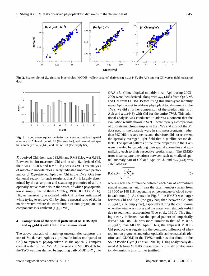
Fig. 2. Scatter plot ofRrs (in situ: blue circles; MODIS: yellow squares) derived(a) at-w(443),(b) Aph and(c) Chl versus field measureddata.

25

Month

1 2 3 4 5 6 7 8 9 10 11 12

RM

SD

0.0

0.4

0.8

1.2

1.6

546 Fig. 3 Root mean square deviation between normalized spatial anomaly of Aph and that of Chl 547

(the grey bar), and normalized spatial anomaly of at-w(443) and that of Chl (the empty bar). 548

549

Fig. 3. Root mean square deviation between normalized spatialanomaly of Aph and that of Chl (the grey bar), and normalized spa-tial anomaly ofat-w(443) and that of Chl (the empty bar).

Rrs derived Chl, theε was 135.6% and RMSElog was 0.383.Between in situ measured Chl and in situRrs derived Chl,the ε was 162.0% and RMSElog was 0.429. This analysisof match-up uncertainties clearly indicated improved perfor-mance ofRrs-retrieved Aph over Chl in the TWS. One fun-damental reason for such results is thatRrs is largely deter-mined by the absorption and scattering properties of all theoptically active materials in the water, of which phytoplank-ton is simply one of them (Mobley, 1994; IOCCG, 2006).Higher uncertainty associated with Chl is thus anticipatedwhile trying to retrieve Chl by simple spectral ratio ofRrs inmarine waters where the contribution of non-phytoplanktoncomponents is significant (e.g., TWS).

4 Comparison of the spatial patterns of MODIS Aphand at-w(443) with Chl in the Taiwan Strait

The above analysis of match-up uncertainties supports theuse ofRrs derived Aph as a preferable index (compared toChl) to represent phytoplankton in the optically complexcoastal water of the TWS. A time series of MODIS Aph forthe TWS was thus derived by inputting daily MODISRrs into

QAA v5. Climatological monthly mean Aph during 2003–2009 were then derived, along withat-w(443) from QAA v5and Chl from OC3M. Before using this multi-year monthlymean Aph dataset to address phytoplankton dynamics in theTWS, we did a further comparison of the spatial patterns ofAph andat-w(443) with Chl for the entire TWS. This addi-tional analysis was conducted to address a concern that theevaluation results shown in Sect. 3 were merely a comparisonof discrete match-up samples in the TWS and most of theRrsdata used in the analysis were in situ measurements, ratherthan MODIS measurements, and, therefore, did not representthe spatially averaged light field that a satellite sensor de-tects. The spatial patterns of the three properties in the TWSwere revealed by calculating their spatial anomalies and nor-malizing each to their respective spatial mean. The RMSD(root mean square deviation) between each normalized spa-tial anomaly pair of Chl and Aph or Chl andat-w(443) wascalculated as:

RMSD=

√√√√1

n

n∑i=1

δ2 (6)

whereδ was the difference between each pair of normalizedspatial anomalies, andn was the pixel number (varies from134 000 to 148 118, depending on percentage of cloud coverin each month). As shown in Fig. 3, the RMSD was largerbetween Chl and Aph (the grey bar) than between Chl andat-w(443) (the empty bar), especially during the cold seasonwhen the wind was strong and the water was relatively turbiddue to sediment resuspension (Guo et al., 1991). This find-ing clearly indicates that the spatial pattern of empiricallyderived MODIS Chl was more similar to that of MODISat-w(443) than MODIS Aph. Thus, the empirical MODISChl product was registering the combined influence of phy-toplankton pigments and other optically active materials (de-tritus and CDOM) in the TWS, similar as that found in theSouth Pacific Gyre (Lee et al., 2010b). Using analytically de-rived Aph from MODIS measurements to study phytoplank-ton dynamics is thus further justified.

www.biogeosciences.net/8/841/2011/ Biogeosciences, 8, 841–850, 2011

846 S. Shang et al.: MODIS observed phytoplankton dynamics in the Taiwan Strait

26

550

(a) 551

Month

1 2 3 4 5 6 7 8 9 10 11 12

a ph(4

43) (

m-1

)

0.00

0.02

0.04

0.06

0.08

0.10

Most variable: nearshore waterLeast variable: deep water

552

(b) 553

Fig. 4 (a) Annual mean standard deviation of Aph; (b) the annual cycle of Aph in the most 554

variable coastline (west of the white line alongshore on Fig. 4a) and least variable deep water(the 555

square at the right bottom of Fig. 4a) areas.556

116.5 117 117.5 118 118.5 119 119.5 120 120.5 121 121.5 12222

22.5

23

23.5

24

24.5

25

25.5

(a)

26

550

(a) 551

Month

1 2 3 4 5 6 7 8 9 10 11 12

a ph(4

43) (

m-1

)

0.00

0.02

0.04

0.06

0.08

0.10

Most variable: nearshore waterLeast variable: deep water

552

(b) 553

Fig. 4 (a) Annual mean standard deviation of Aph; (b) the annual cycle of Aph in the most 554

variable coastline (west of the white line alongshore on Fig. 4a) and least variable deep water(the 555

square at the right bottom of Fig. 4a) areas.556

116.5 117 117.5 118 118.5 119 119.5 120 120.5 121 121.5 12222

22.5

23

23.5

24

24.5

25

25.5

(b)

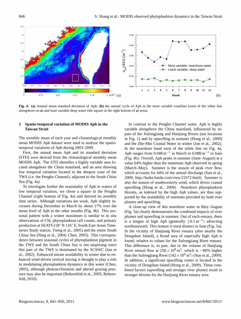
Fig. 4. (a) Annual mean standard deviation of Aph;(b) the annual cycle of Aph in the most variable coastline (west of the white linealongshore ona) and least variable deep water (the square at the right bottom ofa) areas.

5 Spatio-temporal variation of MODIS Aph in theTaiwan Strait

The monthly mean of each year and climatological monthlymean MODIS Aph dataset were used to analyze the spatio-temporal variations of Aph during 2003–2009.

First, the annual mean Aph and its standard deviation(STD) were derived from the climatological monthly meanMODIS Aph. The STD identifies a highly variable area lo-cated alongshore the China mainland, and an area showinglow temporal variation located in the deepest zone of theTWS (i.e. the Penghu Channel), adjacent to the South ChinaSea (Fig. 4a).

To investigate further the seasonality of Aph in waters oflow temporal variation, we chose a square in the PenghuChannel (right bottom of Fig. 4a) and derived its monthlytime series. Although variations are weak, Aph slightly in-creases during December to March by about 17% over themean level of Aph in the other months (Fig. 4b). This sea-sonal pattern with a winter maximum is similar to in situobservations of Chl, phytoplankton cell counts, and primaryproduction at SEATS (18◦ N 116◦ E, South East Asian Time-series Study station, Tseng et al., 2005) and the entire SouthChina Sea (Ning et al., 2004; Chen, 2005). This correspon-dence between seasonal cycles of phytoplankton pigment inthe TWS and the South China Sea is not surprising sincethis part of the TWS is dominated by the SCSWC (Jan etal., 2002). Enhanced nitrate availability in winter due to en-hanced wind-driven vertical mixing is thought to play a rolein modulating phytoplankton dynamics in this water (Chen,2005), although photoacclimation and altered grazing pres-sure may also be important (Behrenfeld et al., 2005; Behren-feld, 2010).

In contrast to the Penghu Channel water, Aph is highlyvariable alongshore the China mainland, influenced by in-puts of the Jiulongjiang and Hanjiang Rivers (see locationsin Fig. 1) and by upwelling in summer (Hong et al., 2009)and the Zhe-Min Coastal Water in winter (Jan et al., 2002).In the nearshore band west of the white line on Fig. 4a,Aph ranges from 0.048 m−1 in March to 0.088 m−1 in June(Fig. 4b). Overall, Aph peaks in summer (June–August) at avalue 64% higher than the minimum Aph observed in spring(March–May). Summer is the season of peak river flow,which accounts for 44% of the annual discharge (Sun et al.,2009;http://baike.baidu.com/view/23372.html). Summer isalso the season of southwesterly wind, which drives coastalupwelling (Hong et al., 2009). Nearshore phytoplanktonblooms, as indexed by the high Aph values, are thus sup-ported by the availability of nutrients provided by both riverplumes and upwelling.

A close-up view of this nearshore water in May–August(Fig. 5a) clearly demonstrates the combined impacts of riverplumes and upwelling in summer. Out of each estuary, thereis a tongue of high Aph (generally≥0.1 m−1) advectingnortheastward. This feature is most distinct in June (Fig. 5a).In the vicinity of Hanjiang River estuary (also nearby theDongshan Island), a broad area of especially high Aph isfound, relative to values for the Jiulongjiang River estuary.This difference is, in part, due to the volume of HanjiangRiver annual flow at 258× 109 m3, which is ∼80% higherthan the Jiulongjiang River (142×109 m3) (Sun et al., 2009).In addition, a significant upwelling center is located in thevicinity of Dongshan Island (Hong et al., 2009). These com-bined factors (upwelling and stronger river plume) result instronger blooms for the Hanjiang River estuary area.

Biogeosciences, 8, 841–850, 2011 www.biogeosciences.net/8/841/2011/

S. Shang et al.: MODIS observed phytoplankton dynamics in the Taiwan Strait 847

27

May

Jun

Jul

Aug

Hanjiang

557 (a) 558

MEI

0.5

1.5

-1.5

-0.5 AB

I (m

-1)

1500

1000

500

Year

Valid

dat

a pe

rcen

t (%

)

40

60

80

ABI

Win

d st

ress

ano

mal

y (N

/M2 )

-0.05

0.00

0.05

2003 2004 2005 2006 200920082007

559

(b) 560

Fig. 5 (a) close-up view of Aph in the nearshore water (west of the white line alongshore on 561

Fig. 4a) in May-August; (b) The interannual variation of Aph percentage of valid retrievals and 562

alongshore wind stress anomaly in the area of Hanjiang River estuary in June during 2003-2009 563

and the MEI. 564

565

566

(a)

27

May

Jun

Jul

Aug

Hanjiang

557 (a) 558

MEI

0.5

1.5

-1.5

-0.5 AB

I (m

-1)

1500

1000

500

Year

Valid

dat

a pe

rcen

t (%

)

40

60

80

ABI

Win

d st

ress

ano

mal

y (N

/M2 )

-0.05

0.00

0.05

2003 2004 2005 2006 200920082007

559

(b) 560

Fig. 5 (a) close-up view of Aph in the nearshore water (west of the white line alongshore on 561

Fig. 4a) in May-August; (b) The interannual variation of Aph percentage of valid retrievals and 562

alongshore wind stress anomaly in the area of Hanjiang River estuary in June during 2003-2009 563

and the MEI. 564

565

566

(b)

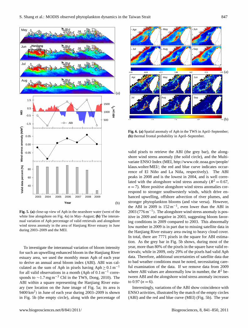
Fig. 5. (a)close-up view of Aph in the nearshore water (west of thewhite line alongshore on Fig. 4a) in May–August;(b) The interan-nual variation of Aph percentage of valid retrievals and alongshorewind stress anomaly in the area of Hanjiang River estuary in Juneduring 2003–2009 and the MEI.

To investigate the interannual variation of bloom intensityfor such an upwelling enhanced bloom in the Hanjiang Riverestuary area, we used the monthly mean Aph of each yearto derive an annual areal bloom index (ABI). ABI was cal-culated as the sum of Aph in pixels having Aph≥ 0.1 m−1

for all valid observations in a month (Aph of 0.1 m−1 corre-sponds to∼1.7 mg m−3 Chl in the TWS, Dong, 2010). TheABI within a square representing the Hanjiang River estu-ary (see location on the June image of Fig. 5a; its area is9400 km2) in June of each year during 2003–2009 is shownin Fig. 5b (the empty circle), along with the percentage of

28

Apr

Sep

May Jun

AugJul

567

(a)568

Apr

Sep

May Jun

AugJul

Apr

Sep

May Jun

AugJul

Apr

Sep

May Jun

AugJul

Apr

Sep

May Jun

AugJul

569

(b) 570

Fig. 6 (a) Spatial anomaly of Aph in the TWS in April-September; (b) thermal frontal 571

probability in April-September. 572

(a)

28

Apr

Sep

May Jun

AugJul

567

(a)568

Apr

Sep

May Jun

AugJul

Apr

Sep

May Jun

AugJul

Apr

Sep

May Jun

AugJul

Apr

Sep

May Jun

AugJul

569

(b) 570

Fig. 6 (a) Spatial anomaly of Aph in the TWS in April-September; (b) thermal frontal 571

probability in April-September. 572

(b)

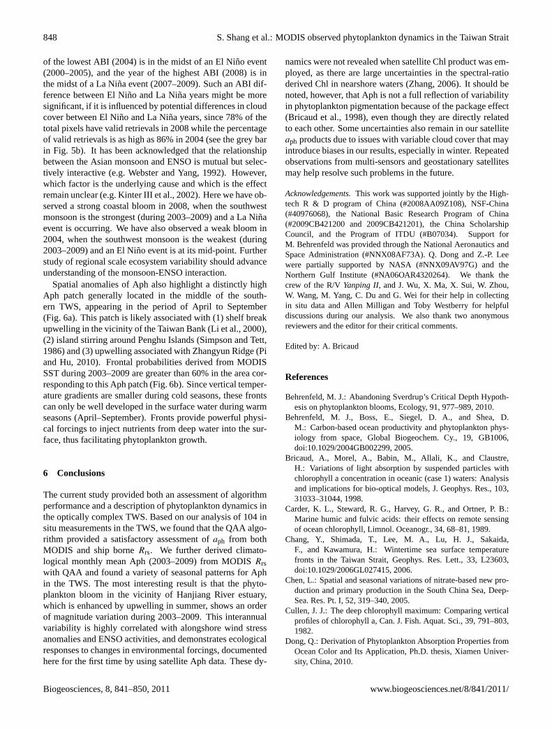
Fig. 6. (a)Spatial anomaly of Aph in the TWS in April–September;(b) thermal frontal probability in April–September.

valid pixels to retrieve the ABI (the grey bar), the along-shore wind stress anomaly (the solid circle), and the Multi-variate ENSO Index (MEI,http://www.cdc.noaa.gov/people/klaus.wolter/MEI/; the red and blue curve indicates occur-rence of El Nino and La Nina, respectively). The ABIpeaks in 2008 and is the lowest in 2004, and is well corre-lated with the alongshore wind stress anomaly (R2

= 0.67,n = 7). More positive alongshore wind stress anomalies cor-respond to stronger southwesterly winds, which drive en-hanced upwelling, offshore advection of river plumes, andstronger phytoplankton blooms (and vise versa). However,the ABI in 2009 is 152 m−1, even lower than the ABI in2003 (776 m−1). The alongshore wind stress anomaly is pos-itive in 2009 and negative in 2003, suggesting bloom favor-ing conditions in 2009 compared to 2003. This abnormallylow number in 2009 is in part due to missing satellite data inthe Hanjiang River estuary area owing to heavy cloud cover.In total, there are 7771 pixels in the square for ABI estima-tion. As the grey bar in Fig. 5b shows, during most of theyear, more than 80% of the pixels in the square have valid re-trievals; while in 2009, only 29% of the pixels had valid Aphdata. Therefore, additional uncertainties of satellite data dueto bad weather conditions must be noted, necessitating care-ful examination of the data. If we remove data from 2009where ABI values are abnormally low in number, theR2 be-tween ABI and the alongshore wind stress anomaly increasesto 0.97 (n = 6).

Interestingly, variations of the ABI show coincidence withENSO activities, illustrated by the match of the empty circles(ABI) and the red and blue curve (MEI) (Fig. 5b). The year

www.biogeosciences.net/8/841/2011/ Biogeosciences, 8, 841–850, 2011

848 S. Shang et al.: MODIS observed phytoplankton dynamics in the Taiwan Strait

of the lowest ABI (2004) is in the midst of an El Nino event(2000–2005), and the year of the highest ABI (2008) is inthe midst of a La Nina event (2007–2009). Such an ABI dif-ference between El Nino and La Nina years might be moresignificant, if it is influenced by potential differences in cloudcover between El Nino and La Nina years, since 78% of thetotal pixels have valid retrievals in 2008 while the percentageof valid retrievals is as high as 86% in 2004 (see the grey barin Fig. 5b). It has been acknowledged that the relationshipbetween the Asian monsoon and ENSO is mutual but selec-tively interactive (e.g. Webster and Yang, 1992). However,which factor is the underlying cause and which is the effectremain unclear (e.g. Kinter III et al., 2002). Here we have ob-served a strong coastal bloom in 2008, when the southwestmonsoon is the strongest (during 2003–2009) and a La Ninaevent is occurring. We have also observed a weak bloom in2004, when the southwest monsoon is the weakest (during2003–2009) and an El Nino event is at its mid-point. Furtherstudy of regional scale ecosystem variability should advanceunderstanding of the monsoon-ENSO interaction.

Spatial anomalies of Aph also highlight a distinctly highAph patch generally located in the middle of the south-ern TWS, appearing in the period of April to September(Fig. 6a). This patch is likely associated with (1) shelf breakupwelling in the vicinity of the Taiwan Bank (Li et al., 2000),(2) island stirring around Penghu Islands (Simpson and Tett,1986) and (3) upwelling associated with Zhangyun Ridge (Piand Hu, 2010). Frontal probabilities derived from MODISSST during 2003–2009 are greater than 60% in the area cor-responding to this Aph patch (Fig. 6b). Since vertical temper-ature gradients are smaller during cold seasons, these frontscan only be well developed in the surface water during warmseasons (April–September). Fronts provide powerful physi-cal forcings to inject nutrients from deep water into the sur-face, thus facilitating phytoplankton growth.

6 Conclusions

The current study provided both an assessment of algorithmperformance and a description of phytoplankton dynamics inthe optically complex TWS. Based on our analysis of 104 insitu measurements in the TWS, we found that the QAA algo-rithm provided a satisfactory assessment ofaph from bothMODIS and ship borneRrs. We further derived climato-logical monthly mean Aph (2003–2009) from MODISRrswith QAA and found a variety of seasonal patterns for Aphin the TWS. The most interesting result is that the phyto-plankton bloom in the vicinity of Hanjiang River estuary,which is enhanced by upwelling in summer, shows an orderof magnitude variation during 2003–2009. This interannualvariability is highly correlated with alongshore wind stressanomalies and ENSO activities, and demonstrates ecologicalresponses to changes in environmental forcings, documentedhere for the first time by using satellite Aph data. These dy-

namics were not revealed when satellite Chl product was em-ployed, as there are large uncertainties in the spectral-ratioderived Chl in nearshore waters (Zhang, 2006). It should benoted, however, that Aph is not a full reflection of variabilityin phytoplankton pigmentation because of the package effect(Bricaud et al., 1998), even though they are directly relatedto each other. Some uncertainties also remain in our satelliteaph products due to issues with variable cloud cover that mayintroduce biases in our results, especially in winter. Repeatedobservations from multi-sensors and geostationary satellitesmay help resolve such problems in the future.

Acknowledgements.This work was supported jointly by the High-tech R & D program of China (#2008AA09Z108), NSF-China(#40976068), the National Basic Research Program of China(#2009CB421200 and 2009CB421201), the China ScholarshipCouncil, and the Program of ITDU (#B07034). Support forM. Behrenfeld was provided through the National Aeronautics andSpace Administration (#NNX08AF73A). Q. Dong and Z.-P. Leewere partially supported by NASA (#NNX09AV97G) and theNorthern Gulf Institute (#NA06OAR4320264). We thank thecrew of the R/VYanping II, and J. Wu, X. Ma, X. Sui, W. Zhou,W. Wang, M. Yang, C. Du and G. Wei for their help in collectingin situ data and Allen Milligan and Toby Westberry for helpfuldiscussions during our analysis. We also thank two anonymousreviewers and the editor for their critical comments.

Edited by: A. Bricaud

References

Behrenfeld, M. J.: Abandoning Sverdrup’s Critical Depth Hypoth-esis on phytoplankton blooms, Ecology, 91, 977–989, 2010.

Behrenfeld, M. J., Boss, E., Siegel, D. A., and Shea, D.M.: Carbon-based ocean productivity and phytoplankton phys-iology from space, Global Biogeochem. Cy., 19, GB1006,doi:10.1029/2004GB002299, 2005.

Bricaud, A., Morel, A., Babin, M., Allali, K., and Claustre,H.: Variations of light absorption by suspended particles withchlorophyll a concentration in oceanic (case 1) waters: Analysisand implications for bio-optical models, J. Geophys. Res., 103,31033–31044, 1998.

Carder, K. L., Steward, R. G., Harvey, G. R., and Ortner, P. B.:Marine humic and fulvic acids: their effects on remote sensingof ocean chlorophyll, Limnol. Oceanogr., 34, 68–81, 1989.

Chang, Y., Shimada, T., Lee, M. A., Lu, H. J., Sakaida,F., and Kawamura, H.: Wintertime sea surface temperaturefronts in the Taiwan Strait, Geophys. Res. Lett., 33, L23603,doi:10.1029/2006GL027415, 2006.

Chen, L.: Spatial and seasonal variations of nitrate-based new pro-duction and primary production in the South China Sea, Deep-Sea. Res. Pt. I, 52, 319–340, 2005.

Cullen, J. J.: The deep chlorophyll maximum: Comparing verticalprofiles of chlorophyll a, Can. J. Fish. Aquat. Sci., 39, 791–803,1982.

Dong, Q.: Derivation of Phytoplankton Absorption Properties fromOcean Color and Its Application, Ph.D. thesis, Xiamen Univer-sity, China, 2010.

Biogeosciences, 8, 841–850, 2011 www.biogeosciences.net/8/841/2011/

S. Shang et al.: MODIS observed phytoplankton dynamics in the Taiwan Strait 849

Dong, Q., Hong, H., and Shang, S.: A new approach to correct forpathlength amplification in measurements of particulate spectralabsorption by the quantitative filter technique, Journal of Xia-men University (Natural Science), 47, 556–561, 2008 (in Chi-nese, with English abstract).

Du, C., Shang, S., Dong, Q., Hu, C., and Wu, J.: Characteristics ofChromophoric Dissolved Organic Matter in the nearshore watersof the western Taiwan Strait, Estuar. Coast. Shelf. S., 88, 350–356, 2010.

Gordon, H. R.: Normalized water-leaving radiance: revisiting theinfluence of surface roughness, Appl. Optics, 44, 241–248, 2005.

Gordon, H. R., Brown, O. B., Evans, R. H., Brown, J. W., Smith,R. C., Baker, K. S., and Clark, D. K.: A semianalytic radiancemodel of ocean color, J. Geophys. Res., 93, 10909–10924, 1988.

Guo, L., Hong, H., Chen, J., and Hong, L.: Distribution and vari-ation of suspended matter in the southern Taiwan Strait, in:Minnan-taiwan bank fishing ground upwelling ecosystem study,edited by: Hong, H., 273–281, 1991 (in Chinese, with Englishabstract).

Hirawake, T., Takao, S., Horimoto, N., Ishimaru, T., Yamaguchi,Y., and Fukuchi, M.: A phytoplankton absorption-based primaryproductivity model for remote sensing in the Southern Ocean,Polar Biol., 34, 291–302, 2011.

Hong, H., Wu, J., Shang, S., and Hu, C.: Absorption and fluo-rescence of chromophoric dissolved organic matter in the PearlRiver Estuary, South China, Mar. Chem., 97, 78–89, 2005.

Hong, H., Zhang, C., Shang, S., Huang, B., Li, Y., Li, X., andZhang, S.: Interannual variability of summer coastal upwellingin the Taiwan Strait, Cont. Shelf. Res., 29, 479–484, 2009.

International Ocean-Colour Coordinating Group (IOCCG): Remotesensing of inherent optical properties: Fundamentals, tests ofalgorithms, and applications, in: Reports of the InternationalOcean-Colour Coordinating Group, No. 5, edited by: Lee, Z.,Dartmouth, Canada, 2006.

Jan, S., Wang, J., Chern, C. S., and Chao, S. Y.: Seasonal variationof the circulation in the Taiwan Strait, J. Marine Syst., 35, 249–268, 2002.

Kiefer, D. A. and SooHoo, J. B.: Spectral absorption by marineparticles of coastal waters of Baja California, Limnol. Oceanogr.,27, 492–499, 1982.

Kinter III, J., Miyakoda, K., and Yang, S.: Recent change in theconnection from the Asian monsoon to ENSO, J. Climate, 15,1203–1215, 2002.

Kishino, M., Takahashi, M., Okami, N., and Ichimura, S.: Estima-tion of the spectral absorption coefficients of phytoplankton inthe sea, B. Mar. Sci., 37, 634–642, 1985.

Lee, Z., Carder, K. L., Marra, J., Steward, R. G., and Perry, M.J.: Estimating primary production at depth from remote sensing,Appl. Optics, 35(2), 463–474, 1996.

Lee, Z., Carder, K. L., and Arnone, R. A.: Deriving inherent opticalproperties from water color: a multiband quasi-analytical algo-rithm for optically deep waters, Appl. Optics, 41, 5755–5772,2002.

Lee, Z., Lubac, B., Werdell, J., and Arnone, R.: An update ofthe Quasi-Analytical Algorithm (QAAv5), available at:http://www.ioccg.org/groups/SoftwareOCA/QAA v5.pdf, 2009.

Lee, Z., Ahn, Y., Mobley, C., and Arnone, R.: Removal ofsurface-reflected light for the measurement of remote-sensing re-flectance from an above-surface platform, Opt. Express, 18(25),

26313–26342, 2010a.Lee, Z., Shang, S., Hu, C., Lewis, M., Arnone, R., Li, Y., and

Lubac, B.: Time series of bio-optical properties in a subtropi-cal gyre: Implications for the evaluation of inter-annual trendsof biogeochemical properties, J. Geophys. Res., 115, C09012,doi:10.1029/2009JC005865, 2010b.

Li, C., Hu, J., Jan, S., Wei, Z., Fang, G. H., and Zheng, Q.: Winter-spring fronts in Taiwan Strait, J. Geophys. Res., 111, C11S13,doi:10.1029/2005JC003203, 2006.

Li, L., Guo, X., and Wu, R.: Oceanic fronts in southern TaiwanStrait, Journal of Oceanography in Taiwan Strait, 19, 147–156,2000 (in Chinese, with English abstract).

Marra, J., Trees, C. C., and O’Reilly, J. E.: Phytoplankton pigmentabsorption: A strong predictor of primary productivity in the sur-face ocean, Deep-Sea. Res. Pt. I, 54, 155–163, 2007.

Melin, F., Zibordi, G., and Berthon, J. F.: Assessment of satelliteocean color products at a coastal site, Remote. Sens. Environ.,110, 192–215, 2007.

Mitchell, B. G., Bricaud, A., and Carder, K.: Determination ofspectral absorption coefficients of particles, dissolved materialand phytoplankton for discrete water samples, in: Ocean op-tics protocols for satellite ocean color sensor validation, revi-sion 2, edited by: Fargion, G. S. and Mueller, J. L., Greenbelt,Maryland: NASA Goddard Space Flight Space Center, 125–153,2000.

Mobley, C. D.: Light and water: Radiative Transfer in Natural Wa-ters, Academic, New York, 1994.

Ning, X., Chai, F., Xue, H., Cai, Y., Liu, C., and Shi, J.: Physical-biological oceanographic coupling influencing phytoplanktonand primary production in the South China Sea, J. Geophys. Res.,109, C10005,doi:10.1029/2004JC002365, 2004.

O’Reilly, J. E., Maritorena, S., Siegel, D., and O’Brien, M. C.:Ocean color chlorophyll a algorithms for SeaWiFS, OC2, andOC4: version 4, in: SeaWiFS postlaunch technical report se-ries, volume 11, SeaWiFS postlaunch calibration and validationanalyses, part 3, edited by: Hooker, S. B. and Firestone, E. R.,Greenbelt, Maryland: NASA Goddard Space Flight Center, 9–23, 2000.

Pi, Q. and Hu, J.: Analysis of sea surface temperature fronts in theTaiwan Strait and its adjacent area using an advanced edge de-tection method, Science China, Earth Sci., 53, 1008–1016, 2010.

Sathyendranath, S., Hoge, F. E., Platt, T., and Swift, R. N.: De-tection of phytoplankton pigments from ocean color: Improvedalgorithms, Appl. Optics, 33, 1081–1089, 1994.

Simpson, J. H. and Tett, P.: Island steering effects on phytoplanktongrowth, in: Lecture notes on coastal and estuarine studies, editedby: Bowman, J., Yentsch, M., and Peterson, W. T., Berlin, 41–76,1986.

Stewart, R. H.: Introduction to physical oceanography, Departmentof Oceanography, Texas A & M University, 2008.

Stuart, V., Sathyendranath, S., Platt, T., Maass, H., and Irwin, B.:Pigments and species composition of natural phytoplankton pop-ulations: effect on the absorption spectra, J. Plankton Res., 20,187–217, 1998.

Sun, B., Zhou, G., Wei, H., Liu, Z., and Zeng, D.: The flux of riveractive material flowing into the sea: Preliminary achievements,Earth Science Frontiers, 16, 361–368, 2009 (in Chinese, withEnglish abstract).

Tassan, S. and Ferrari, G. M.: An alternative approach to absorption

www.biogeosciences.net/8/841/2011/ Biogeosciences, 8, 841–850, 2011

850 S. Shang et al.: MODIS observed phytoplankton dynamics in the Taiwan Strait

measurements of aquatic particles retained on filters, Limnol.Oceanogr., 40, 1358–1368, 1995.

Tassan, S. and Ferrari, G. M.: A sensitivity analysis of the“Transmittance-Reflectance” method for measuring light absorp-tion by aquatic particles, J. Plankton. Res., 24, 757–774, 2002.

Tseng, C. M., Wong, G. T. F., Lin, I. I., Wu, C. R., and Liu, K. K.: Aunique seasonal pattern in phytoplankton biomass in low-latitudewaters in the South China Sea, Geophys. Res. Lett., 32, L08608,doi:10.1029/2004GL022111, 2005.

Wang, D. X., Liu, Y., Qi, Y. Q., and Shi, P.: Seasonal variabilityof thermal fronts in the northern South China Sea from satellitedata, Geophys. Res. Lett., 28, 3963–3966, 2001.

Webster, P. and Yang, S.: Monsoon and ENSO: Selectively interac-tive systems, Q. J. Roy. Meteor. Soc., 118, 877–926, 1992.

Westberry, T., Behrenfeld, M. J., Siegel, D. A., and Boss, E.:Carbon-based primary productivity modeling with vertically re-solved photoacclimation, Global. Biogeochem. Cy., 22, GB2024,doi:10.1029/2007GB003078, 2008.

Yelland, M. J. and Taylor, P. K.: Wind stress measurements fromthe open ocean, J. Phys. Oceanogr., 26, 541–558, 1996.

Yelland, M. J., Moat, B. I., Taylor, P. K., Pascal, R. W., Hutch-ings, J., and Cornell, V. C.: Wind stress measurements from theopen ocean corrected for airflow distortion by the ship, J. Phys.Oceanogr., 28, 1511–1526, 1998.

Zhang, C., Hu, C., Shang, S., Muller-Karger, F. E., Li, Y., Dai, M.,Huang, B., Ning, X., and Hong, H.: Bridging between SeaW-iFS and MODIS for continuity of chlorophyll-a concentration as-sessments off Southeastern China, Remote. Sens. Environ., 102,250–263, 2006.

Zhang, C. Y.: Response of chlorophyll a to marine environmentvariability on multiple time scales in the Taiwan Strait, Ph.D.dissertation, Xiamen University, China, 2006.

Biogeosciences, 8, 841–850, 2011 www.biogeosciences.net/8/841/2011/