Modifying coalChemistryFoam for dense gas-solid simulation

Cite as: Zhang, J.: Modifying coalChemistryFoam for dense gas-solid simulation. In Proceedings of CFD

with OpenSource Software, 2018, Edited by Nilsson. H., http://dx.doi.org/10.17196/OS_CFD#YEAR_2018

CFD with OpenSource software

A course at Chalmers University of TechnologyTaught by Hakan Nilsson

Modifying coalChemistryFoam for densegas-solid simulation

Developed for OpenFOAM-v1806Requires: coalChemistryFoam

Author:Jingyuan ZhangNorwegian University ofScience and [email protected]

Peer reviewed by:Ebrahim Ghahramani

Marcus Jansson

Licensed under CC-BY-NC-SA, https://creativecommons.org/licenses/

Disclaimer: This is a student project work, done as part of a course where OpenFOAM and someother OpenSource software are introduced to the students. Any reader should be aware that it

might not be free of errors. Still, it might be useful for someone who would like learn some detailssimilar to the ones presented in the report and in the accompanying files. The material has gone

through a review process. The role of the reviewer is to go through the tutorial and make sure thatit works, that it is possible to follow, and to some extent correct the writing. The reviewer has no

responsibility for the contents.

December 22, 2018

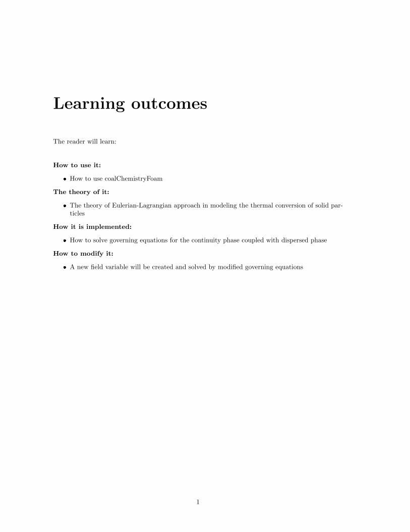
Learning outcomes

The reader will learn:

How to use it:

� How to use coalChemistryFoam

The theory of it:

� The theory of Eulerian-Lagrangian approach in modeling the thermal conversion of solid par-ticles

How it is implemented:

� How to solve governing equations for the continuity phase coupled with dispersed phase

How to modify it:

� A new field variable will be created and solved by modified governing equations

1

Prerequisites

The reader is expected to know the following in order to get maximum benefit out of this report:

� Fundamentals of Eulerian-Lagrangian approach in simulating gas-solid system

� How to run standard document tutorials like coalChemistryFoam tutorial

2

Preface

In OpenFOAM-v1806 the Lagrangian solvers are coalChemistryFoam, DPMFoam, simpleCoalParcelFoam, reactingParcelFoam, sprayFoam, icoUncoupledKinematicParcleFoam and UncoupledKine

maticParcleFoam. (solvers like DPMDyMFoam are not listed, because they are extensions of relevantsolvers. For example, DyM means dynamic mesh in DPMDyMFoam). Not only the particle modelsfor the Lagrangian tracking solid phase are different, but also the coupling methods between thecontinuous phase and the dispersed phase are distinguishable. The last two mentioned solvers, forcompressible and incompressible fluid, are not two-way coupling and require a pre-calculated veloc-ity field. The rest, except DPMFoam, are for compressible fluid. As for the coupling method, onlyDPMFoam considers the effects of the volume fraction of particles on the continuous phase. In addi-tion, simpleCoalParcel is a steady state solver.

In the simulation of the thermal conversion of solid particles, the porous media model is widely used.It requires averaging methods when modeling the solid phase, and it has difficulties in simulatingparticles individual behaviours and interactions. In order to include more physics, the Eulerian-Lagrangian approach could be a better option. In the situation that the solid phase is quite dense,such as in grate fire furnace, we prefer to take both compressibility and effects of volume fractionof particles into account. In this respective, we need to modify the existing Lagrangian solvers inOpenFOAM.

In this tutorial, a new solver coalChemistryAlphaFoam will be developed based on coalChemistryFo

am. The difference between the new solver and the original one is that the effects of the volumefraction of particles will be considered. The first section is theory and introduction, and then adetail understanding of the source code of coalChemistryFoam will be given. The third part is theimplementation of the new solver, as well as a tutorial about how to modify the solvers. At last asample test case will be conducted to show how to use the new solver.

3

Contents

1 Theoretical Background of Eulerian-Lagrangian Approach 5

2 coalChemistryFoam 72.1 Governing equations for the gas phase . . . . . . . . . . . . . . . . . . . . . . . . . . 72.2 Walkthrough of the source code . . . . . . . . . . . . . . . . . . . . . . . . . . . . . . 7

2.2.1 coalChemistryFoam.C . . . . . . . . . . . . . . . . . . . . . . . . . . . . . . . 82.3 How the equations are solved . . . . . . . . . . . . . . . . . . . . . . . . . . . . . . . 11

2.3.1 rhoEqn.H . . . . . . . . . . . . . . . . . . . . . . . . . . . . . . . . . . . . . . 112.3.2 UEqn.H . . . . . . . . . . . . . . . . . . . . . . . . . . . . . . . . . . . . . . . 122.3.3 YEqn.H . . . . . . . . . . . . . . . . . . . . . . . . . . . . . . . . . . . . . . . 132.3.4 EEqn.H . . . . . . . . . . . . . . . . . . . . . . . . . . . . . . . . . . . . . . . 14

2.4 Pressure correction . . . . . . . . . . . . . . . . . . . . . . . . . . . . . . . . . . . . . 152.4.1 PIMPLE algorithm . . . . . . . . . . . . . . . . . . . . . . . . . . . . . . . . . 152.4.2 pEqn.H . . . . . . . . . . . . . . . . . . . . . . . . . . . . . . . . . . . . . . . 16

2.5 Submodels . . . . . . . . . . . . . . . . . . . . . . . . . . . . . . . . . . . . . . . . . . 172.5.1 createFields.H . . . . . . . . . . . . . . . . . . . . . . . . . . . . . . . . . . . 18

3 coalChemistryAlphaFoam 193.1 New governing euqations . . . . . . . . . . . . . . . . . . . . . . . . . . . . . . . . . . 193.2 Implementation . . . . . . . . . . . . . . . . . . . . . . . . . . . . . . . . . . . . . . . 20

3.2.1 Alpha fields . . . . . . . . . . . . . . . . . . . . . . . . . . . . . . . . . . . . . 203.2.2 coalChemistryTurbulenceModel . . . . . . . . . . . . . . . . . . . . . . . . . . 223.2.3 Modification of the equations in the code . . . . . . . . . . . . . . . . . . . . 263.2.4 Completion of the solver . . . . . . . . . . . . . . . . . . . . . . . . . . . . . . 29

4 Sample case 314.1 Preparing the case . . . . . . . . . . . . . . . . . . . . . . . . . . . . . . . . . . . . . 314.2 Results . . . . . . . . . . . . . . . . . . . . . . . . . . . . . . . . . . . . . . . . . . . . 33

4

Chapter 1

Theoretical Background ofEulerian-Lagrangian Approach

In Eulerian-Lagrangian approach, the continuous phase is treated as a continuum by solving theNavier-Stokes equations and the conservation equations (strictly speaking, Navier-Stokes equationsare the momentum equation for viscous fluid, but in some papers we can also see that people useNavier-Stokes equations also including the mass and heat balance equations. Here we prefer the gen-eralized definition.), and the dispersed phase is calculated by tracking of a large number of particleswhich follow the Newton’s second law. In modeling granular flows, discrete element method (DEM)and Discrete Phase Model (DPM) are the models under Eulerian-Lagrangian framework. There isno strict distinction between DPM and DEM. DEM emphasize on the collision between individualparticles, while DPM stresses the particles behaviour as a group.

When deriving the governing equations for the continuous phase in multi-phase flow systems, howto deal with the averaging method and coupling between the different phases will result in differentformulations. According to the different ways of the decomposition of particle-fluid interaction forceterm in the governing equations for the continuous phase, the momentum equations are classifiedinto models A and B [1].

The equation set of model A is

∂αρcu

∂t+∇ · (αρcuu) = −α∇p− FA + α∇ · τ + αρcg (1.1)

where α is fluid volume phase fraction, ρc is fluid phase density, g is gravity, τ is deviatoric stresstensor and FA is the volumetric particle-fluid interaction force. In model A, the interaction forcecontains drag force fd,i and the rest particle-fluid interaction forces, i stands for the individualparticle label.

FA =1

∆V

n∑i=1

(fd,i + f′′

i ) (1.2)

The total particle-fluid interaction force on an individual particle f should include pressure gradientforce f∇p,i (which also includes buoyancy force) and viscous force f∇·τ,i, and can be written as

fA = fd,i + f∇p,i + f∇·τ,i + f′′

i (1.3)

Similar to model A,the equation set according to model B is

∂αρcu

∂t+∇ · (αρcuu) = −∇p− FB +∇ · τ + αρcg (1.4)

5

CHAPTER 1. THEORETICAL BACKGROUND OF EULERIAN-LAGRANGIAN APPROACH

FB =1

∆V

n∑i=1

(fd,i + f∇p,i + f∇·τ,i + f′′

i ) (1.5)

fB = fd,i + f∇p,i + f∇·τ,i + f′′

i (1.6)

Model B is most commonly used as another simplified equation set. The equation for the fluid isthe same as in original model B, except that the particle-fluid interaction force terms are different.The simplified one is

FB∗ =1

α∆V

n∑i=1

(fd,i + f′′

i ) +1

∆V

n∑i=1

(ρcVp,ig) (1.7)

fB∗ =(fd,i + f

′′

i )

α− ρcVp,ig (1.8)

where Vp,i is the particle volume, and this simplification is conditional [1]. It is valid when

αρc[∂u

∂t+∇ · (uu)] = 0 (1.9)

For all of the equation sets above, the ”rest particle-fluid interaction forces” usually includes virtualmass force fvm,i, Basset force fB,i and lift forces such as the Saffman force fSaff,i and Magnus forcefMag,i.

f′′

i = fvm,i + fB,i + fSaff,i + fMag,i (1.10)

While in this work, we are focusing on the gas-solid flow, as compared with drag force these forcecan be neglect.

Although model A and B have different equation forms, both of them are correct and mathe-matically equivalent[2]. The equations here are only the momentum equations without source term.If there are mass transfer between fluid and particles, it will usually rise a momentum source orsink term for the momentum equations. In this tutorial case, during the conversion of the solidparticle, product gas will be released which results a source term. Besides the momentum equation,the mass balance, heat transport, as well as the species transport equations need to be solved. Ifthe turbulence models are used, the governing equations should also include turbulence transportequations. These equations will be given with the certain problems in the following chapters.

6

Chapter 2

coalChemistryFoam

In this chapter, the implementation of coalChemistryFoam in OpenFOAM will be described.

2.1 Governing equations for the gas phase

In coalChemistryFoam the influence of the solid volume fraction is not included. The gas phase iscompressible fluid. The continuity equation in differential form is

∂(ρg)

∂t+∇ · (ρgUg) = Sm (2.1)

The momentum equation is given by

∂(ρgUg)

∂t+∇ · (ρgUgUg)−∇ · (τg)−∇ · (ρgRg) = −∇p+ ρgg + SU (2.2)

The energy transport equation is

∂(ρgh)

∂t+∂(ρgK)

∂t+∇ · (ρgUgh) +∇ · (ρgUgK)−∇ ·

(αeff∇(h)

)= ∇p+ ρgUg · g + Sh (2.3)

Species transport equation is

∂(ρgYi)

∂t+∇ · (ρgUgYi)−∇ ·

(Deff∇(ρgYi)

)= Si (2.4)

S are the source terms, Rg is Ronald stress term, h is the enthalpy, K is kinetic energy, Yi is themass fraction of the species. αeff and Deff are the effective thermal and mass diffusivity, and”effective” means it include turbulent diffusivity when turbulence model is used.

2.2 Walkthrough of the source code

The coalChemistryFoam solver files are located in :

$FOAM_SOLVERS/lagrangian/coalChemistryFoam

We are going to have a deep looking into all the files. The walkthrough of the code is a tutorialon how the equations are implemented into code. The solver will start with the main file, whichis coalChemistryFoam.C. All the other files in this folder are included in the main file. Then theequations files will be explained. We will try to find every terms from the equations in the code. Nextis the createFields.H, at the same time, the mechanism of runtime selection (RTS) will be brieflyintroduced. The rest of the files in the directory will be introduced in the coalChemistryFoam.C

and createFields.H section.

7

2.2. WALKTHROUGH OF THE SOURCE CODE CHAPTER 2. COALCHEMISTRYFOAM

coalChemistryFoam

|

|---Make

| |---files

| |---options

|

|---coalChemistryFoam.C

|---createClouds.H

|---createFieldRefs.H

|---createFields.H

|---EEqn.H

|---pEqn.H

|---rhoEqn.H

|---setDeltaT.H

|---UEqn.H

|---YEqn.H

2.2.1 coalChemistryFoam.C

We all know that OpenFOAM is just a C++ code package, and this C file is where the code starts.First, before the main function, there is a block of included the header files.

#include "fvCFD.H"

#include "turbulentFluidThermoModel.H"

#include "basicThermoCloud.H"

#include "coalCloud.H"

#include "psiReactionThermo.H"

#include "CombustionModel.H"

#include "fvOptions.H"

#include "radiationModel.H"

#include "SLGThermo.H"

#include "pimpleControl.H"

#include "pressureControl.H"

#include "localEulerDdtScheme.H"

#include "fvcSmooth.H"

These header files defines the classes and types needed by finite volume method, turbulent model,physical properties, combustion model, PIMPLE algorithm and so on. These are ”real” headerfiles, which are just declarations. It will be an endless work if we want to dig into every H file. Wecan go back to them to find the hierarchy relations of the classes, if we need to figure out the details.

Then we can go into main() function. The main function starts with including another blockof H files.

{

#include "postProcess.H"

#include "addCheckCaseOptions.H"

...

#include "initContinuityErrs.H"

These are certain code segment instead of ”real” header files. We will have a quick look on each fileand come back to them when we need details.

#include "postProcess.H"

Execute application functionObjects to post-process results.

8


#include "addCheckCaseOptions.H"

#include "setRootCase.H"

#include "createTime.H"

#include "createMesh.H"

These four files are located in $FOAM_SRC/OpenFOAM/include folder, and they are the basic initialsettings for starting a new case.

addCheckCaseOptions.H includes predefined arguments to check case set-up.

setRootCase.H will create an object from argList class to register and output informations ac-cording the case settings. argList is a very basic class defined in argList.H, and its function is toextract command arguments and options from the inputs.

createTime.H will create the object runtime from the Time class. This class is used to controltime loops during the calculation.

createMesh.H will create the object mesh from the fvMesh class. fvMesh is a multiple inheritenceclass, and it inherits from polyMesh class and other classes related to finite volume method.

#include "createControl.H"

createControl.H is located in $FOAM_SRC/finiteVolume/cfdTools/general/solutionControl.In createControl.H three different solver controllers are defined (SIMPLE, PISO and PIMPLE). IncoalChemistryFoam, PIMPLE algorithm is used. The three algorithm control classes are inheritedfrom the solutionControl class, while solutionControl is inherited from IOobject class. Thesealgorithm control class will supply convergence information checks for the calculation loop. Theimplementation of pressure correction algorithm is usually in the pEqn.H file.

#include "creatTimeControls.H"

creatTimeControls.H is located in $FOAM_SRC/finiteVolume/cfdTools/general/include Threevariables adjustTimeStep, maxCo and maxDeltaT will be created and initialized from the controlDict.

#include "createFields.H"

In this file, the variables are created as fields data object. It is worth to notice that it also includesnew H files, and defined two pointer variables which in OpenFOAM are from autoPrt templatetype. The two pointers are combustion for combustion model and turbulent for turbulence model.The pointer created by New function is using for the ”Run Time Selection(RTS)” method, it allowsto select the submodel class used in template after compiling of the source code. We will look intomore detail in this file in the following sections.

#include createFieldRefs.H"

This file will create a reference field, if the inertia species are defined.

#include initContinuityErrs.H

Declare and initialise the cumulative continuity error.

Now the object and variable declaration is almost done. Before the calculation, check the turbulentmodel by following code.

turbulence->validate();

Before entering the time loop, set initial time step and calculate Co number.

9


if (!LTS)

{

#include "compressibleCourantNo.H"

#include "setInitialDeltaT.H"

}

// * * * * * * * * * * * * * * * * * * * * * * * * * * //

Info<< "\nStarting time loop\n" << endl;

while (runTime.run())

{

#include "readTimeControls.H"

if (LTS)

{

#include "setRDeltaT.H"

}

else

{

#include "compressibleCourantNo.H"

#include "setDeltaT.H"

}

runTime++;

Info<< "Time = " << runTime.timeName() << nl << endl;

If the adjust time step model turns on, each time step during the time loop is determined by theCourant number. LTS is short for local time stepping. When the reactions and radiation model isactivated, LTS is usually used. It needs to be specified according to the solver itself, so we can findthe file ”setDeltaT.H” in the solver’s directory.

In fact a lot of such universal code segments are made into H files, and are located in $FOAM_SRC/fini

teVolume/ or $FOAM_SRC/OpenFOAM/ directories. However, in some solvers these files need to bemodified. Then the modified H files will be provided in the same folder as the C file, where thecompiler will look for firstly. It is good to check whether we need to modify such universal H files,when we doing changes to a solver.

Then, the solver calculates and updates particles’ parameter by calling the evolve() function inthe parcel class, the source terms from the particle to the gas phase equations will also be calcu-lated. rhoEffLagrangian and pDyn is not used in the calculation. They are only calculated forpost-process.

rhoEffLagrangian = coalParcels.rhoEff() + limestoneParcels.rhoEff();

pDyn = 0.5*rho*magSqr(U);

coalParcels.evolve();

limestoneParcels.evolve();

Next, solve the governing eqautions for the gas phase, and correct the pressure using PIMPLEalgorithm.

#include "rhoEqn.H"

// --- Pressure-velocity PIMPLE corrector loop

10

2.3. HOW THE EQUATIONS ARE SOLVED CHAPTER 2. COALCHEMISTRYFOAM

while (pimple.loop())

{

#include "UEqn.H"

#include "YEqn.H"

#include "EEqn.H"

// --- Pressure corrector loop

while (pimple.correct())

{

#include "pEqn.H"

}

Calculate the effective viscosity and diffusivity by calling the turbulence model’s correct function.The ”effective” includes turbulent contributions. The laminar viscosity and diffusivity will be cal-culated first. In OpenFOAM, the laminar model is also united into turbulence models. It meansthat we should choose the turbulence model as laminar if no turbulence models are used.

if (pimple.turbCorr())

{

turbulence->correct();

}

}

At last, the density of the gas phase is updated according to the ”equation of state” model, andwrite data before entering the next time step.

rho = thermo.rho();

runTime.write();

}

The main code ends here with return 0;. We know roughly how the solver is designed, now weneed to go into more details.

2.3 How the equations are solved

In OpenFOAM the finite volume method is used. We will go into the equation files to see how thegoverning equations are implemented in the code.

2.3.1 rhoEqn.H

In rhoEqn.H the continuity equation is defined as:

fvScalarMatrix rhoEqn

(

fvm::ddt(rho)

+ fvc::div(phi)

==

coalParcels.Srho(rho)

+ fvOptions(rho)

);

The variable phi in OpenFOAM is usually the flux, and it is a surfaceScalarField, which meansit is calculated by interpolation from cell centre values. In different solvers, it could be mass flux orvolumetric flux. In createFields.H, by including compressibleCreatePhi.H, phi is defined as:

11


linearInterpolate(rho*U) & mesh.Sf()

The code coalParcels.Srho(rho) will return the mass source term from the coal parcel, andfvOptions(rho) will operate user-defined calculation. If nothing add, this term can be neglect fromthe equation.

Doing integration of Eq. 2.1 by volume, we get∫V

[∂ρg∂t

+∇ · (ρgUg)

]dV =

∫V

[Sm] dV (2.5)

For term∫V∇ · (ρgUg)dV , we use Gauss theorem. For one cell, the integration of the surfaces is

calculated by the summation of all of the cell faces, we can get∫V

∇ · (ρgUg)dV =

∮∂V

(ρgUg) · dS =∑f

∫Sf

(ρgUg) · dSf =∑f

(ρgUg)f · Sf (2.6)

So the mass balance equation 2.1 for one cell with a volume of V becomes:

∂ρg∂t

V +∑f

(ρgUg)f · Sf = SmV (2.7)

Now we get every term in the code corresponding to Eq. 2.7. Calling the solve() function to solvethe equation, the density rho will be updated according to continuity.

rhoEqn.solve();

fvOptions.correct(rho);

2.3.2 UEqn.H

In UEqn.H The momentum equation is defined as:

fvVectorMatrix UEqn

(

fvm::ddt(rho, U) + fvm::div(phi, U)

+ MRF.DDt(rho, U)

+ turbulence->divDevRhoReff(U)

==

rho()*g

+ coalParcels.SU(U)

+ limestoneParcels.SU(U)

+ fvOptions(rho, U)

);

MRF is for rotating reference frame, MRF.DDt will return the contribution from the rotating referenceframe effects. divDevRhoReff(U) function is determined by the turbulence model. It will returnthe source term for the momentum equation. This source term only includes the viscosity term andReynolds stress term. For example, if a turbulence model except laminar model is used, the functiondefined in $FOAM_SRC/TurbulenceModels/turbulenceModels/ReynoldsStress/ReynoldsStress.C

will be called, and if the couplingFactor is 0 (in all the OpenFOAM tutorial cases, couplingFactoris 0. It will weight the explicit calculation of the Reynold stress term, and details could be found inthe definition), the return value of divDevRhoReff is defined as:

fvc::laplacian

(

this->alpha_*rho*this->nut(),

12


U,

"laplacian(nuEff,U)"

)

+ fvc::div(this->alpha_*rho*R_)

- fvc::div(this->alpha_*rho*this->nu()*dev2(T(fvc::grad(U))))

- fvm::laplacian(this->alpha_*rho*this->nuEff(), U)

alpha_ is the phase fraction. In coalChemistryFoam, it is not considered. Thereby its value is1. nut() is the turbulent viscosity calculated from turbulence model. nuEff() is the summationof laminar viscosity and turbulent viscosity. R is Reynold stress tensor and the calculation ofdev2(T(fvc::grad(U))) equals to

dev2((∇U)T ) = (∇U)T − 2

3tr((∇U)T )I = (∇U)T − 2

3(∇ ·U)I (2.8)

In OpenFOAM, the operation fvc will calculate the results as the source term, so we can regard thefvc term as explicit term. However, the fvm will return the discrete matrix coefficient, and it makethe fvm term as implicit term. We can interpret the code of the definition of divDevRhoReff intothe following equation

[∇ · (νtρ∇U) +∇ · (ρR)−∇ · (νρ(∇U)T − 2

3νρ(∇ ·U)I)]explicit − [∇ · ((ν + νt)ρ∇U)]implicit

= −[∇ · (νρ∇U)]implicit − [∇ · (νρ(∇U)T − 2

3νρ(∇ ·U)I)]explicit + [∇ · (ρR)]explicit

+ [∇ · (νtρ∇U)]explicit − [∇ · (νtρ∇U)]implicit (2.9)

here ν is laminar viscosity and νt is turbulent viscosity. The equation above is just the ∇ · (τg) +∇ · (ρgRg) term using Stokes assumption is the momentum equation 2.2. For the convection term∇ · (ρgUgUg), again use Gauss theorem like we did in the mass balance equation above, we get∫

V

∇ · (ρgUgUg)dV =

∮∂V

(ρgUgUg) · dS =∑f

∫Sf

(ρgUgUg) · dSf

=∑f

(ρgUgUg)f · Sf ≈∑f

Ug((ρgUg)f · Sf ) (2.10)

Now compared with Eq.2.2, we have found every term except the pressure term. How to couple themomentum equation with the pressure correction is always not a easy problem. In coalChemistryFoam

the PIMPLE algorithm is used. First we predict the velocity and use PIMPLE algorithm to correctthe pressure and velocity; it will be explained later. After applying relaxation factor and fvOptions,the velocity is predicted for PIMPLE loop.

if (pimple.momentumPredictor())

{

solve(UEqn == -fvc::grad(p));

fvOptions.correct(U);

K = 0.5*magSqr(U);

}

K, the (specific) kinetic energy is also calculated for the energy calculation.

2.3.3 YEqn.H

In the YEqn.H file, a convectionScheme, which is named mvConvection, is defined at the beginning.It is created on free store in random-access memory (RAM). When the number of gas species is large,it enhances the computational efficiency.

13


tmp<fv::convectionScheme<scalar>> mvConvection

(

fv::convectionScheme<scalar>::New

(

mesh,

fields,

alphaRhoPhic,

mesh.divScheme("div(alphaRhoPhi,Yi_h)")

)

);

Before calculate the species transport equation, the gas phase combustion is calculated and the heateffects of the reactions is stored in the parameter Qdot().

combustion->correct();

Qdot = combustion->Qdot();

A variable Yt is initialized and used in the calculation loop to make sure all the species mass fractiontogether is 1. The error is made up by the inert gas. The transport equation is defined as:

fvScalarMatrix YiEqn

(

fvm::ddt(rho, Yi)

+ mvConvection->fvmDiv(phi, Yi)

- fvm::laplacian(turbulence->muEff(), Yi)

==

coalParcels.SYi(i, Yi)

+ combustion->R(Yi)

+ fvOptions(rho, Yi)

);

With the analysis above, it is very strait forword the equation 2.4. It is important to update theboundary condition after solving the equation:

fvOptions.constrain(YiEqn);

2.3.4 EEqn.H

The energy equation solves for the enthalpy of the gas species (Eq. 2.3). The kinetic energy is alsoadded in the equation as explicit terms. The enthalpy h could also be internal energy e. The energytransport equation will be similar except for the pressure-volume work term, so there are two wayto solve the energy equation. The code of the equation is defined as:

fvScalarMatrix EEqn

(

fvm::ddt(rho, he) + mvConvection->fvmDiv(phi, he)

+ fvc::ddt(rho, K) + fvc::div(phi, K)

+ (

he.name() == "e"

? fvc::div

(

fvc::absolute(phi/fvc::interpolate(rho), U),

p,

"div(phiv,p)"

)

: -dpdt

)

14

2.4. PRESSURE CORRECTION CHAPTER 2. COALCHEMISTRYFOAM

- fvm::laplacian(turbulence->alphaEff(), he)

==

rho*(U&g)

+ Qdot

+ coalParcels.Sh(he)

+ limestoneParcels.Sh(he)

+ radiation->Sh(thermo, he)

+ fvOptions(rho, he)

);

alphaEff() returns the effective turbulent thermal diffusivity for enthalpy. The code is also quitedirect to be implemented from Eq. 2.3. After solving the energy equation, the thermal physicalproperties will be updated according to the new temperature, and the radiation will be calculated.

thermo.correct();

radiation->correct();

2.4 Pressure correction

In the velocity equation, the velocity needs to be solved together by the pressure correction. IncoalChemistryFoam PIMPLE algorithm is used. To have a better understanding of the solver, abrief review of PIMPLE algorithm will be given first, then the implementation in pEqn.H will beexplained.

2.4.1 PIMPLE algorithm

The PIMPLE Algorithm is a combination of PISO (Pressure Implicit with Splitting of Operator)and SIMPLE (Semi-Implicit Method for Pressure-Linked Equations). It is used for the transientcase. The calculation scheme in one time step of PIMPLE Algorithm is:

� From the momentum equation predict the velocity U .

� Discrete momentum equation without the pressure term.

APUP +∑

ANUN − E = 0, (2.11)

here subscript P is the current cell and N is the neighbour cells, and E includes the sourceterm. A new velocity can be calculated by adding the pressure gradient as:

U∗P =1

AP(∑

ANUN − E −∇p) = HbyA∗ − 1

AP∇p (2.12)

� U∗P should satisfy the continuity equation, and get pressure correction. For example if thecontinuity equation is ∇ · U = 0, then

∇ ·U∗P = ∇ · (HbyA∗ − 1

AP∇p) = 0 (2.13)

� Calculate pressure (for collocated mesh, Rhie-Chow interpolation may be used), and correctthe velocities with the new pressure field.

� Return to step 2, until velocity is converged.

15

2.4. PRESSURE CORRECTION CHAPTER 2. COALCHEMISTRYFOAM

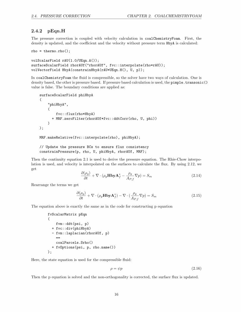
2.4.2 pEqn.H

The pressure correction is coupled with velocity calculation in coalChemistryFoam. First, thedensity is updated, and the coefficient and the velocity without pressure term HbyA is calculated:

rho = thermo.rho();

volScalarField rAU(1.0/UEqn.A());

surfaceScalarField rhorAUf("rhorAUf", fvc::interpolate(rho*rAU));

volVectorField HbyA(constrainHbyA(rAU*UEqn.H(), U, p));

In coalChemistryFoam the fluid is compressible, so the solver have two ways of calculation. One isdensity based, the other is pressure based. If pressure based calculation is used, the pimple.transonic()value is false. The boundary conditions are applied as:

surfaceScalarField phiHbyA

(

"phiHbyA",

(

fvc::flux(rho*HbyA)

+ MRF.zeroFilter(rhorAUf*fvc::ddtCorr(rho, U, phi))

)

);

MRF.makeRelative(fvc::interpolate(rho), phiHbyA);

// Update the pressure BCs to ensure flux consistency

constrainPressure(p, rho, U, phiHbyA, rhorAUf, MRF);

Then the continuity equation 2.1 is used to derive the pressure equation. The Rhie-Chow interpo-lation is used, and velocity is interpolated on the surfaces to calculate the flux. By using 2.12, weget

∂(ρg)

∂t+∇ · (ρgHbyA∗f −

ρgAP,f

∇p) = Sm (2.14)

Rearrange the terms we get

∂(ρg)

∂t+∇ · (ρgHbyA∗f )−∇ · ( ρg

AP,f∇p) = Sm (2.15)

The equation above is exactly the same as in the code for constructing p equation

fvScalarMatrix pEqn

(

fvm::ddt(psi, p)

+ fvc::div(phiHbyA)

- fvm::laplacian(rhorAUf, p)

==

coalParcels.Srho()

+ fvOptions(psi, p, rho.name())

);

Here, the state equation is used for the compressible fluid:

ρ = ψp (2.16)

Then the p equation is solved and the non-orthogonality is corrected, the surface flux is updated.

16

2.5. SUBMODELS CHAPTER 2. COALCHEMISTRYFOAM

pEqn.solve(mesh.solver(p.select(pimple.finalInnerIter())));

if (pimple.finalNonOrthogonalIter())

{

phi = phiHbyA + pEqn.flux();

}

Next, the continuity is constrained by calculating Eq. 2.1 again. The velocity is corrected accordingto the new calculated pressure, and at last, the kinetic energy and the energy term due to pressureare also updated for the energy calculation.

U = HbyA - rAU*fvc::grad(p);

U.correctBoundaryConditions();

fvOptions.correct(U);

K = 0.5*magSqr(U);

if (thermo.dpdt())

{

dpdt = fvc::ddt(p);

}

If the density based calculation is used, the density in the second term of the Eq. 2.15 should alsobe replaced by the state equation.

2.5 Submodels

We have seen how the equations are solved in coalChemistryFoam. To have a better understandingof the code, another important part is essential, which is how the submodels are coupled with thesolver. Noticing that in the solvers folder, there are only two files we haven’t look at, createClouds.Hand createFields.H. createClouds.H is included in createFields.H, and it includes the decla-ration of the particle classes. It is worth to mention that the particles are solved at different levels.The most basic is particle class, then particles with the same properties sharing the same calculationform parcels, and a cloud can include many parcels.

In the definition of submodels object, RTS mechanism is used. In fact, RTS is widely used inOpenFOAM. Here a brief introduction of RTS is described before we go into createFields.H file.

RTS makes it possible to construct a derived class using a base class as its interface. It is designedto have the function of ”virtual constructor function”, because in C++ the constructor function cannot be a virtual function. It will be too complicated to explain it in detail, which is also beyond thescope of this tutorial. Since we are trying to understand the code, so the basic step to implementRTS for a set of class is described as

� In the base class, use macro declareRunTimeSelectionTable to create a hash table as a staticmember. In this table, all the elements are pairs of key-value terms. The key is the name ofthe derived class which is generated by typeName function following the OpenFOAM namingrules, and the value is a pointer pointing to the constructor function of the derived class.

� Every time that a derived class is defined from the base class, the derived class will use macroaddToRunTimeSelectionTable to add a key-value of its name and constructor function pointerto the hash table.

� During compiling, the hashTable will be updated, and will contain all the derived class.

17

2.5. SUBMODELS CHAPTER 2. COALCHEMISTRYFOAM

� In the base class a New function is defined as a static member, and its type is also a pointerautoPtr. It can receive the augments and return the pointer to constructor of the selectedderived class from the hash table. Then the RTS is realized, an object of the derived class iscreated using a base class pointer.

2.5.1 createFields.H

In this H files, it includes several other H files.

#include "createRDeltaT.H"

#include "readGravitationalAcceleration.H"

#include "compressibleCreatePhi.H"

#include "createDpdt.H"

#include "createK.H"

#include "createMRF.H"

#include "createClouds.H"

#include "createRadiationModel.H"

#include "createFvOptions.H"

They are just code segments and by the name of the H files we can easily tell the function of thesefiles. For example, createRDeltaT.H is used to create reciprocal local face time-step field for LTSmodel, and compressibleCreatePhi.H is the flux times the density by interpolation method. Bothof them are already mention above.

The variables are defined, and some are defined with the argument IOobject. IOobject is moreconvenient to control the input and output of the variables. There are also three pointers that aredefined as autoPtr.

Info<< "Reading thermophysical properties\n" << endl;

autoPtr<psiReactionThermo> pThermo(psiReactionThermo::New(mesh));

...

Info<< "Creating turbulence model\n" << endl;

autoPtr<compressible::turbulenceModel> turbulence

(

compressible::turbulenceModel::New

(

rho,

U,

phi,

thermo

)

);

Info<< "Creating combustion model\n" << endl;

autoPtr<CombustionModel<psiReactionThermo>> combustion

(

CombustionModel<psiReactionThermo>::New(thermo, turbulence())

);

They are all initialized with a New functions. The RTS mention above is used here. The thermo-physical model, turbulence model and combustion model are then coupled into the solver.

18

Chapter 3

coalChemistryAlphaFoam

In this chapter a solver based on coalChemistryFoam is developed. The solid volume fraction isconsidered by adding the gas phase volume fraction α to the governing equations in the new solver.First, the new governing equations will be given, then the changes to the code will be made to solvethe new equations.

3.1 New governing euqations

According to the theory background in chapter 1, the equation for fluid-particle system have two dif-ferent model in formulation. The difference lies in the decomposition of the particle-fluid interactionforce. Please notice that the different drag force in OpenFOAM have different forms. Basically if theforce models are changed the modified solver may not be strictly valid in the governing equations.In this case, the governing equations for the gas phase need to be adjust. Here we use the settingsin the tutorial case for coalChemistryFoam, where the particle force is set as:

particleForces

{

sphereDrag;

gravity;

}

The source codes to calculate parcel force are in the $FOAM_SRC/lagrangian/intermediate/submodels/Kinematic/ParticleForces folder. The drag force is coupled to the Eulerian governing equa-tions while the gravity is uncoupled. The buoyancy force is also included in the gravity. ”Uncou-pled” means it does not have any contribution in the fluid momentum equation. It will be easierto use model A to implement. The f

′′

i term in 1.2 is neglected, which is acceptable. While for theparticle, the buoyancy force is part of f∇p,i, and the rest force is also neglected. It is also reasonable,because the drag force and gravity are dominating the particle motion. Then we can get the set ofthe new governing equations.

The continuity equation is∂(αρg)

∂t+∇ · (αρgUg) = Sm (3.1)

The momentum equation

∂(αρgUg)

∂t+∇ · (αρgUgUg)−∇ · (ατg)−∇ · (αρgRg) = −α∇p+ αρgg + SU (3.2)

The energy transport equation is

∂(αρg(h+K))

∂t+∇ · (αρgUg(h+K))−∇ ·

(ααeff∇(h)

)= α∇p+ αρgUg · g + Sh (3.3)

19

3.2. IMPLEMENTATION CHAPTER 3. COALCHEMISTRYALPHAFOAM

Species transport equation is

∂(αρgYi)

∂t+∇ · (αρgUgYi)−∇ ·

(αDeff∇(ρgYi)

)= Si (3.4)

From the chapter 2 we have seen how the equations are implemented into the code. For the newsolver, the surface flux needs to be modified by multiplying the phase volume fraction. There aretwo main tasks. The first one is the Laplace diffusion terms is calculated from the turbulence model,and it means a new turbulence models is required to take the volume fraction of the gas phase intoaccount. The second one is that the pressure correction needs to be specified according to the newequations.

3.2 Implementation

The new solver coalChemistryAlphaFoam is modified on coalChemistryFoam. The implementationfollows the step below:

� Create the new fields variables.

� Create the new turbulence model.

� Update the calculation of the equations

Before beginning, we should prepare the solver. Go to the user directory (or the directory preferred),copy coalChemistryFoam to the folder and rename it to coalChemistryAlphaFoam.

cp -r $FOAM_APP/solvers/lagrangian/coalChemistryFoam .

mv coalChemistryFoam/ coalChemistryAlphaFoam/

cd coalChemistryAlphaFoam/

Rename the C file, and redirect the compiling to user bin folder

mv coalChemistryFoam.C coalChemistryAlphaFoam.C

sed -i s/coalChemistryFoam/coalChemistryAlphaFoam/g Make/files

sed -i s/FOAM_APPBIN/FOAM_USER_APPBIN/g Make/files

3.2.1 Alpha fields

In the createFields.H file, replace the code #include "compressibleCreatePhi.H" with the fol-lowing code:

surfaceScalarField phi

(

IOobject

(

"phi",

runTime.timeName(),

mesh,

IOobject::READ_IF_PRESENT,

IOobject::AUTO_WRITE

),

linearInterpolate(U) & mesh.Sf()

);

The old H file will create the mass surface flux, but we need volumetric flux in the new solver. Thenadd the following code after #include "createClouds.H":

20


volScalarField alpha

(

IOobject

(

"alpha",

runTime.timeName(),

mesh,



),

mesh,

dimensionedScalar(dimless, Zero)

);

scalar alphaMin

(

1.0

- readScalar

(

coalParcels.particleProperties()

.subDict("constantProperties").lookup("alphaMax")

)

);

alpha = max(1.0 - coalParcels.theta() - limestoneParcels.theta(), alphaMin);

alpha.correctBoundaryConditions();

surfaceScalarField alphaf("alphaf", fvc::interpolate(alpha));

Info<<"alphaf: "<<alphacf<<endl;

surfaceScalarField rhoPhi

(

IOobject

(

"rhoPhi",

runTime.timeName(),

mesh,



),

fvc::interpolate(rho)*phi

);

surfaceScalarField alphaRhoPhi

(

IOobject

(

"alphaRhoPhi",

runTime.timeName(),

mesh,



),

alphaf*rhoPhi

21


);

The alpha fields is defined, as well as the phase fraction weighted surface flux is. Notes that aminimum value of alpha is needed. This value should be provided in the coalParcels dictionary,in the constantProperties subDict, by name of alphaMax, the value should be (1 - alphaMin).

3.2.2 coalChemistryTurbulenceModel

The turbulent model used in coalChemistryFoam is defined in the createClouds.H file:

autoPtr<compressible::turbulenceModel> turbulence

(

compressible::turbulenceModel::New

(

rho,

U,

phi,

thermo

)

)

The compressible::turbulenceModel is defined in the file $FOAM_SRC/TurbulenceModels/compressible/turbulentFluidThermoModels/turbulentFluidThermoModel.H

namespace compressible

{

typedef ThermalDiffusivity<CompressibleTurbulenceModel<fluidThermo>>

turbulenceModel;

...

This model is in the library libcompressibleTurbulenceModels.so. From the code we can see thatthe class fluidThermo is used as the type of transport model. The turbulence model is inherited fromCompressibleTurbulenceModel, while we prefer to use PhaseCompressibleTurbulenceModel. Theproblem is that there is no library that instantiated the template PhaseCompressibleTurbulenceModelwith class fluidThermo, so we need to compile a new library first. (To make such a library, thy wayto make similar libraries in multiphase solvers can be used as references).

First, at the new solver directory create a sub-directory for the library of turbulence Model. Interminal using the following command:

mkdir coalChemistryTurbulenceModels

Then create three files to use macro to instantiate the template class.

touch coalChemistryTurbulenceModels/coalChemistryTurbulenceModel.H

touch coalChemistryTurbulenceModels/coalChemistryTurbulenceModelFwd.H

touch coalChemistryTurbulenceModels/coalChemistryTurbulenceModels.C

Add the following code to coalChemistryTurbulenceModel.H file

#ifndef coalChemistryTurbulenceModel_H

#define coalChemistryTurbulenceModel_H

#include "coalChemistryTurbulenceModelFwd.H"

#include "PhaseCompressibleTurbulenceModel.H"

#include "ThermalDiffusivity.H"

#include "fluidThermo.H"

22


// * * * * * * * * * * * * * * * * * * * * * * * * * * * * * * * * * * * * * //

namespace Foam

{

typedef ThermalDiffusivity<PhaseCompressibleTurbulenceModel<fluidThermo>>

coalChemistryTurbulenceModel;

}

// * * * * * * * * * * * * * * * * * * * * * * * * * * * * * * * * * * * * * //

#endif

Add the following code to coalChemistryTurbulenceModelFwd.H file

#ifndef coalChemistryTurbulenceModelFwd_H

#define coalChemistryTurbulenceModelFwd_H

// * * * * * * * * * * * * * * * * * * * * * * * * * * * * * * * * * * * * * //

namespace Foam

{

class fluidThermo;

template<class TransportModel>

class PhaseCompressibleTurbulenceModel;

template<class BasicTurbulenceModel>

class ThermalDiffusivity;

typedef ThermalDiffusivity<PhaseCompressibleTurbulenceModel<fluidThermo>>

coalChemistryTurbulenceModel;

}

// * * * * * * * * * * * * * * * * * * * * * * * * * * * * * * * * * * * * * //

#endif

However, this file is not necessary, it is also OK to do not have this file. It just makes the codefollow the structure in OpenFOAM.

Add the following code to coalChemistryTurbulenceModels.C file

#include "PhaseCompressibleTurbulenceModel.H"

#include "fluidThermo.H"

#include "addToRunTimeSelectionTable.H"

#include "makeTurbulenceModel.H"

#include "ThermalDiffusivity.H"

#include "EddyDiffusivity.H"

#include "laminarModel.H"

#include "RASModel.H"

#include "LESModel.H"

// * * * * * * * * * * * * * * * * * * * * * * * * * * * * * * * * * * * * * //

23


makeTurbulenceModelTypes

(

volScalarField,

volScalarField,

compressibleTurbulenceModel,

PhaseCompressibleTurbulenceModel,

ThermalDiffusivity,

fluidThermo

);

makeBaseTurbulenceModel

(

volScalarField,

volScalarField,

compressibleTurbulenceModel,

PhaseCompressibleTurbulenceModel,

ThermalDiffusivity,

fluidThermo

);

#define makeLaminarModel(Type) \

makeTemplatedLaminarModel \

(fluidThermoPhaseCompressibleTurbulenceModel, laminar, Type)

#define makeRASModel(Type) \

makeTemplatedTurbulenceModel \

(fluidThermoPhaseCompressibleTurbulenceModel, RAS, Type)

#define makeLESModel(Type) \

makeTemplatedTurbulenceModel \

(fluidThermoPhaseCompressibleTurbulenceModel, LES, Type)

#include "Stokes.H"

makeLaminarModel(Stokes);

#include "kEpsilon.H"

makeRASModel(kEpsilon);

#include "kOmegaSST.H"

makeRASModel(kOmegaSST);

#include "Smagorinsky.H"

makeLESModel(Smagorinsky);

#include "kEqn.H"

makeLESModel(kEqn);

Only five turbulence models are added here. If other models are preferred, just add the new modelusing makeLaminar/RAS/LESModel macros.

Then make rules to compile the library. In terminal using command:

mkdir coalChemistryTurbulenceModels/Make

touch coalChemistryTurbulenceModels/Make/files

touch coalChemistryTurbulenceModels/Make/options

24


In files add:

coalChemistryTurbulenceModels.C

LIB = $(FOAM_USER_LIBBIN)/libcoalChemistryTurbulenceModels

In options add:

EXE_INC = \

-I$(LIB_SRC)/transportModels/compressible/lnInclude \

-I$(LIB_SRC)/thermophysicalModels/basic/lnInclude \

-I$(LIB_SRC)/transportModels/incompressible/transportModel \

-I$(LIB_SRC)/TurbulenceModels/compressible/lnInclude \

-I$(LIB_SRC)/TurbulenceModels/turbulenceModels/lnInclude \

-I$(LIB_SRC)/TurbulenceModels/phaseCompressible/lnInclude \

-I$(LIB_SRC)/finiteVolume/lnInclude \

-I$(LIB_SRC)/meshTools/lnInclude

LIB_LIBS = \

-lcompressibleTransportModels \

-lfluidThermophysicalModels \

-lspecie \

-lturbulenceModels \

-lcompressibleTurbulenceModels \

-lincompressibleTransportModels \

-lfiniteVolume \

-lfvOptions \

-lmeshTools

Since the new library will be used, we should add the new library into the options file of the newsolver. After EXE_INC = \, add:

-I../coalChemistryAlphaFoam/coalChemistryTurbulenceModels \

After -I$(LIB_SRC)/TurbulenceModels/compressible/lnInclude \, add:

-I$(LIB_SRC)/TurbulenceModels/phaseCompressible/lnInclude \

-I$(LIB_SRC)/transportModels \

After EXE_LIBS = \, add:

-L$(FOAM_USER_LIBBIN) \

After -lphaseCompressibleTurbulenceModels \, add:

-lcoalChemistryTurbulenceModels \

Now we can use the new turbulence model in the new solver. Again in the createClouds.H file,replace the declaration of the turbulence pointer with the following code:

autoPtr<coalChemistryTurbulenceModel> turbulence

(

coalChemistryTurbulenceModel::New

(

alpha,

rho,

U,

alphaRhoPhi,

phi,

thermo

)

);

25


Then the new turbulence model can take the phase volume fraction into account.

3.2.3 Modification of the equations in the code

The modification of the equations in the code is quite straightforward to the new governing equations.For the mass balance equation in the rhoEqn.H, the code should be changed into:

fvScalarMatrix rhoEqn

(

fvm::ddt(alpha, rho)

+ fvc::div(alphaRhoPhi)

==

coalParcels.Srho(rho)

+ fvOptions(rho)

);

For the UEqn.H, the code should be changed into:

fvVectorMatrix UEqn(U, rho.dimensions()*U.dimensions()*dimVol/dimTime);

UEqn =

(

fvm::ddt(alpha, rho, U) + fvm::div(alphaRhoPhi, U)

+ MRF.DDt(alpha*rho, U)

+ turbulence->divDevRhoReff(U)

==

alpha*rho()*g

+ coalParcels.SU(U)

+ limestoneParcels.SU(U)

+ fvOptions(rho, U)

);

While inside the momentumPredictor, the pressure should be multiply by the phase fraction

solve(UEqn == -alpha*fvc::grad(p));

For the YEqn.H, firstly, the surface mass flux should be corrected by the phase fraction:

tmp<fv::convectionScheme<scalar>> mvConvection

(

fv::convectionScheme<scalar>::New

(

mesh,

fields,

alphaRhoPhi,

mesh.divScheme("div(alphaRhoPhi,Yi_h)")

)

);

Then, according to Eq. 3.4, the governing equation should be modified as

const volScalarField muEff(turbulence->muEff());

forAll(Y, i)

{

if (i != inertIndex && composition.active(i))

{

volScalarField& Yi = Y[i];

26


fvScalarMatrix YiEqn

(

fvm::ddt(alpha, rho, Yi)

+ mvConvection->fvmDiv(alphaRhoPhi, Yi)

- fvm::laplacian

(

fvc::interpolate(alpha)

*fvc::interpolate(muEff),

Yi

)

==

coalParcels.SYi(i, Yi)

+ combustion->R(Yi)

+ fvOptions(rho, Yi)

);

...

The EEqn.H, according to Eq. 3.3, should be modified as

const volScalarField alphaEff(turbulence->alphaEff());

fvScalarMatrix EEqn

(

fvm::ddt(alpha, rho, he) + mvConvection->fvmDiv(alphaRhoPhi, he)

+ fvc::ddt(alpha, rho, K) + fvc::div(alphaRhoPhi, K)

+ (

he.name() == "e"

? fvc::div

(

fvc::absolute(alphaRhoPhi/fvc::interpolate(rho), U),

p,

"div(phiv,p)"

)

: -dpdt*alpha

)

- fvm::laplacian

(

fvc::interpolate(alpha)

*fvc::interpolate(alphaEff),

he

)

==

alpha*rhoc*(U&g)

+ Qdot

+ coalParcels.Sh(he)

+ limestoneParcels.Sh(he)

+ radiation->Sh(thermo, he)

+ fvOptions(rho, he)

);

As for pressure correction, the pressure equation is derived from the continuity equation 3.1. Forthe new solver the equation should be:

∂(αρg)

∂t+∇ · (αρgHbyA∗f )−∇ · ( αρg

AP,fα∇p) = Sm (3.5)

27


For the modified code, when pimple.transonic() value is false,the code should be like:

else

{

surfaceScalarField phiHbyA

(

"phiHbyA",

(

fvc::flux(rho*HbyA)

+ MRF.zeroFilter(alphaf*rhorAUf*fvc::ddtCorr(rho, U, rhoPhi))

)

);

if (p.needReference())

{

adjustPhi(phiHbyA, U, p);

}

MRF.makeRelative(fvc::interpolate(rho), phiHbyA);

// Update the pressure BCs to ensure flux consistency

constrainPressure(p, rho, U, phiHbyA, rhorAUf, MRF);

while (pimple.correctNonOrthogonal())

{

fvScalarMatrix pEqn

(

fvm::ddt(alpha, psi, p)

+ fvc::div(alphaf*phiHbyA)

- fvm::laplacian(alphaf*alphaf*rhorAUf, p)

==

coalParcels.Srho()


);



{

rhoPhi = phiHbyA + pEqn.flux()/alphaf;

phi = rhoPhi/fvc::interpolate(rho);

}

}

}

And when the case pimple.transonic() is true, which is very unlikely for coal combustion case,the code should be

surfaceScalarField phid

(

"phid",

fvc::interpolate(psi)

*(

fvc::flux(HbyA)

28


+ MRF.zeroFilter

(

rhorAUf*fvc::ddtCorr(rho, U, rhoPhi)/fvc::interpolate(rho)

)

)

);

MRF.makeRelative(fvc::interpolate(psi), phid);

while (pimple.correctNonOrthogonal())

{

fvScalarMatrix pEqn

(

fvm::ddt(alpha, psi, p)

+ fvm::div(alphaf*phid, p)

- fvm::laplacian(alphaf*alphaf*rhorAUf, p)

==

coalParcels.Srho()


);



{

rhoPhi = pEqn.flux()/alphaf;

phi = rhoPhi/fvc::interpolate(rho);

}

}

At the ending, the surface flux need to be updated, and the velocity is calculated from the correctedpressure.

alphaRhoPhi = alphaf*rhoPhi;

U = HbyA - rAU*alpha*fvc::grad(p);

3.2.4 Completion of the solver

Here are some final steps to complete the modification of the solver. The First is to include theturbulence model in the main file, and to update the phase fraction in every time step. After#include "turbulent FluidThermoModel.H" , add the H file

#include "coalChemistryTurbulenceModel.H"

After calculating the parcels ”limestoneParcels.evolve();”, add the following code before ”#include "rhoEqn.H"”to update the phase fraction

alpha = max(1.0 - coalParcel.theta(), alphaMin);

alpha.correctBoundaryConditions();

alphaf = fvc::interpolate(alpha);

alphaRhoPhi = alphaf*rhoPhi;

Because we changed the flux phi from mass flux into volume flux, we need to modify some of theH files included from general source code. For the existing setRDeltaT.H file, change the codecalculated with phi (line 61-65)into:

29


rDeltaT.ref() =

(

fvc::surfaceSum(mag(phi))()()

/((2*maxCo)*mesh.V())

);

Copy two files to the solver folder. In terminal using command:

cp $FOAM_SRC/finiteVolume/cfdTools/compressible/compressibleContinuityErrs.H .

cp $FOAM_SRC/finiteVolume/cfdTools/compressible/compressibleCourantNo.H .

In the file compressibleContinuityErrs.H , change line 33 as:

volScalarField contErr(fvc::ddt(alpha, rho) + fvc::div(alphaRhoPhi) -

coalParcels.Srho(rho)) ;↪→

And in file compressibleCourantNo.H, change the calculation of sumPhi into the following code:

scalarField sumPhi

(

fvc::surfaceSum(mag(rhoPhi))().primitiveField()/rho.primitiveField()

);

The code modification is finished. Compile the coalChemistryTurbulenceModels first, and thencompile the solver. Use the command coalChemistryAlphaFoam to run the solver.

30

Chapter 4

Sample case

The new solver just changed the coupling calculations between the particles and the gas phase, sothe tutorial case for coalChemistryFoam, simplifiedSiwek, could also be used as the sample case.However, some modification should be made for the settings.

4.1 Preparing the case

First go to the directory where is preferred to run the case, for example $FOAM_RUN. Copy thesimplifiedSiwek case to the current folder, and rename it to simplifiedAlphaSiwek , using thecommands

cp -r $FOAM_TUTORIALS/lagrangian/coalChemistryFoam/simplifiedSiwek .

mv simplifiedSiwek simplifiedAlphaSiwek

In the file constant/coalCloud1Properties, add the maximum solid phase fraction in the constant-Properties subDict, after "constantVolume true;":

alphaMax 0.99;

In the file system/controlDict, change the application name into coalChemistryAlphaFoam.

In the file system/fvSchemes, replace the divSchemes into the following code:

{

default none;

div(alphaRhoPhi,U) Gauss upwind;

div((alphaf*phid),p) Gauss upwind;

div(alphaRhoPhi,K) Gauss linear;

div(alphaRhoPhi,h) Gauss upwind;

div(alphaRhoPhi,k) Gauss upwind;

div(alphaRhoPhi,epsilon) Gauss upwind;

div(U) Gauss linear;

div((((alpha*rho)*nuEff)*dev2(T(grad(U))))) Gauss linear;

div(alphaRhoPhi,Yi_h) Gauss upwind;

}

In the original tutorial case, the solid volume fraction is too small. In order to have a more suitabletest case, the diameters of the limestone particles are increased by 10 times, and at the same timethe density is reduced by 100 times. It is of course not practical, and it is just used to test the solver.In the constant/limestoneCloud1Properties file, the code is modified as

31

4.1. PREPARING THE CASE CHAPTER 4. SAMPLE CASE

constantProperties

{

parcelTypeId 2;

rho0 25;

...

}

subModels

{

...

injectionModels

{

...

model1

{

...

sizeDistribution

{

type RosinRammler;

RosinRammlerDistribution

{

minValue 5e-05;

maxValue 0.00565;

d 4.8e-04;

n 0.5;

}

}

}

}

...

}

The number of injected limestone particles is also increased by 3 times by add more injecting position.Another 36 positions shown as follows are added to the constant/limestonePositions file.

(0.0075 0.50 0.05)

(0.0125 0.50 0.05)

(0.0175 0.50 0.05)

(0.0225 0.50 0.05)

(0.0275 0.50 0.05)

(0.0325 0.50 0.05)

(0.0375 0.50 0.05)

(0.0425 0.50 0.05)

(0.0475 0.50 0.05)

(0.0075 0.40 0.05)

(0.0125 0.40 0.05)

(0.0175 0.40 0.05)

(0.0225 0.40 0.05)

(0.0275 0.40 0.05)

(0.0325 0.40 0.05)

(0.0375 0.40 0.05)

(0.0425 0.40 0.05)

(0.0475 0.40 0.05)

32

4.2. RESULTS CHAPTER 4. SAMPLE CASE

(0.0075 0.52 0.05)

(0.0125 0.52 0.05)

(0.0175 0.52 0.05)

(0.0225 0.52 0.05)

(0.0275 0.52 0.05)

(0.0325 0.52 0.05)

(0.0375 0.52 0.05)

(0.0425 0.52 0.05)

(0.0475 0.52 0.05)

(0.0075 0.47 0.05)

(0.0125 0.47 0.05)

(0.0175 0.47 0.05)

(0.0225 0.47 0.05)

(0.0275 0.47 0.05)

(0.0325 0.47 0.05)

(0.0375 0.47 0.05)

(0.0425 0.47 0.05)

(0.0475 0.47 0.05)

4.2 Results

Run the script Allrun, in terminal using:

./Allrun

The same case is also run by the coalChemistryFoam solver as a comparison.

rhoEffLagrangian, which shows the particles concentration for the first written time step in figurebelow shows that the movement of the particle is already different at beginning. It shows thatvelocity fields predicted by the two solvers have notable difference.

33


(a) coalChemistryFoam (b) coalChemistryAlphaFoam

Figure 4.1: rhoEffLagrangian at first written time step

Compared together with the gas phase volume fraction distribution and the pressure profile, itshows that coalChemistryAlphaFoam is more likely to predict a relatively higher pressure gradientat high solid volume fraction region. It is as expected that the local pressure field around theparticles will be more uneven when considering the phase volume fraction effects.

34


(a) coalChemistryFoam (b) coalChemistryAlphaFoam

Figure 4.2: Pressure at 0.5s

Figure 4.3: Gas phase volume fraction

35

References

[1] Zhou, Z. Y., Kuang, S. B., Chu, K. W., & Yu, A. B. (2010). Discrete particle simulation ofparticle–fluid flow: model formulations and their applicability. Journal of Fluid Mechanics, 661,482-510.

[2] Leboreiro, J. (2008). Influence of drag laws on segregation and bubbling behavior in gas-fluidizedbeds (Doctoral dissertation, Ph. D. Thesis, University of Colorado, Boulder, USA).

36

Study questions

� 1. How does the solver get the physical properties like the viscosity of the fluid?

� 2. Why we have to set a minimum fluid volume fraction?

� 3. In one time step, where is the velocity calculated?

� 4. Why should we make a library when we want to use PhaseCompressibleTurbulenceModel?

37

Documents

Modifying coalChemistryFoam for dense gas-solid simulation