Embed Size (px)
Citation preview

UPU.S. Geolo
MtPCSB
T UU
Prepared i
MODFthe SuPackaChapter 23 oSect ion ABook 6, M
Technique
U.S. DepartU.S. Geolog
gical Survn cooperat
FLOW ubsideage (Sof A, Ground W
odeling Te
s and Met
ment of the ical Survey
vey Groundtion with t
Grouence a
SUB-W
Water, of echniques
hods 6–A2
Interior
d-Water Rethe Central
nd-Waand Aq
WT) for
s
3
esources Pl Arizona W
ater Mquiferr Wate
rogram Water Cons
Model—r-Systeer-Tab
servation D
—Useem Cole Aqu
District
r Guidompacuifers
de to ction
Cover illustration: The pressure diagram is figure 3 of the classic paper “Land subsidence due to withdrawal of fluids,” by J.F. Poland and G.H. Davis, Reviews in Engineering Geology II, 1969. For their work on this paper, the authors were given the 1972 O.E. Meinzer Award of the Geological Society of America.

U.S. Geological Survey Ground-Water Resources Program Prepared in cooperation with the Central Arizona Water Conservation District
MODFLOW Ground-Water Model—User Guide to the Subsidence and Aquifer-System Compaction Package (SUB-WT) for Water-Table Aquifers
By S.A. Leake and D.L. Galloway
Techniques and Methods 6–A23
U.S. Department of the Interior U.S. Geological Survey

ii
U.S. Department of the Interior DIRK KEMPTHORNE, Secretary
U.S. Geological Survey Mark D. Myers, Director
U.S. Geological Survey, Reston, Virginia: 2007
For product and ordering information: World Wide Web: http://www.usgs.gov/pubprod Telephone: 1-888-ASK-USGS
For more information on the USGS—the Federal source for science about the Earth, its natural and living resources, natural hazards, and the environment: World Wide Web: http://www.usgs.gov Telephone: 1-888-ASK-USGS
Suggested citation: Leake, S.A., and Galloway, D.L., 2007, MODFLOW ground-water model—User guide to the Subsidence and Aquifer-System Compaction Package (SUB-WT) for water-table aquifers: U.S. Geological Survey, Techniques and Methods 6–A23, 42 p.
Any use of trade, firm, or product names is for descriptive purposes only and does not imply endorsement by the U.S. Government

iii
Contents
Abstract ................................................................................................................................................................................ 1 Introduction ......................................................................................................................................................................... 2 Acknowledgments .............................................................................................................................................................. 3 Theory ................................................................................................................................................................................... 4 Incorporating Interbed Storage into the Ground-Water Flow Equations ................................................................ 9
Thickness of Interbeds ................................................................................................................................................ 10 Average Elevation of Interbeds .................................................................................................................................. 11 Geostatic Stress ............................................................................................................................................................ 11 Effective Stress ............................................................................................................................................................. 12 Preconsolidation Stress .............................................................................................................................................. 12 Storage Properties ....................................................................................................................................................... 13 Void Ratio ....................................................................................................................................................................... 13
Package Output ................................................................................................................................................................ 14 Input Instructions ............................................................................................................................................................. 19
Explanation of Variables Read by the SUB-WT Package .............................................................................. 20 Practical Considerations for Using the SUB-WT Package ....................................................................................... 29
Compatibility of the SUB-WT Package with Versions of MODFLOW.................................................................. 29 Simulation of Flow in and Compaction of Confining Units .................................................................................... 29 Use of Steady-State Stress Periods in MODFLOW ................................................................................................ 30
Sample Simulation ............................................................................................................................................................ 31 Applicability, Assumptions and Limitations ................................................................................................................. 36 References Cited .............................................................................................................................................................. 36 Appendix: Input Data for Sample Simulation .............................................................................................................. 38
MODFLOW Name File .................................................................................................................................................. 38 Basic Package, Version 6 (BA6) Input Data Set ..................................................................................................... 38 Discretization File (DIS) Input Data Set .................................................................................................................... 39 Layer Property-Property Flow Package (LPF) Input Data Set .............................................................................. 40 Well Package (WEL) Input Data Set .......................................................................................................................... 40 Strongly Implicit Procedure Package (SIP) Input Data Set .................................................................................. 41 Output Control Option (OC) Input Data Set ............................................................................................................... 41 Subsidence and Aquifer-System Compaction Package (SUB-WT) for Water-Table Aquifers Input Data Set .................................................................................................................................................................................... 42

iv
Figures Figure 1. Vertical section of a two-aquifer system with potential for compaction of fine-grained sediments. A, Hydrogeology of the system. B, Representation of the system with three model layers. ................................ 2 Figure 2. Stress diagrams for water-table decline with a stable underlying confined aquifer, and for stable water table with head decline in an underlying confined aquifer. ............................................................................ 5 Figure 3. Series of three records needed to specify output for an example simulation using the SUB-WT Package. ............................................................................................................................................................................. 17 Figure 4. Plan view of model domain showing active and inactive areas, and locations of recharge cells, constant-head cells, and wells. ..................................................................................................................................... 32 Figure 5. Generalized section along model row 9 showing types of fine-grained sediments, model layering, and properties and conditions used in the example simulation.Aquifer-system properties and other conditions are listed in figure 5. For simplicity, all material and hydraulic properties and conditions are constant within each model layer or interbed system. ............................................................................................. 33 Figure 6. Computed stresses for row 9, column 10 in example simulation. A, Effective and preconsolidation stress in layer 1, B, geostatic stress in layer 1, C, effective and preconsolidation stress in layer 2, and D, geostatic stress in layer 2. .............................................................................................................................................. 34 Figure 7.. Computed downward vertical displacement for tops of model layers 1-4 at A, location of row 10, column 9, and B, location of row 12, column 7. ........................................................................................................... 35
Tables Table 1. Properties used to compute stresses shown in figure 2 and table 2. ....................................................... 6 Table 2. Computed stresses at two depth horizons (a and b) shown in figure 2. .................................................. 7 Table 3. Information optionally printed or saved by the SUB-WT Package and associated variable names, numbers of arrays, and array names. ........................................................................................................................... 16

v
Conversion Factors Multiply By To obtain
Length
meter (m) 3.281 foot (ft)
kilometer (km) 0.6214 mile (mi)
Volume
cubic meter (m3) 35.31 cubic foot (ft3)
Flow rate
cubic meter per day (m3/d) 35.31 cubic foot per day (ft3/d)
Hydraulic conductivity
meter per day (m/d) 3.281 foot per day (ft/d)
Unit Weight
newton per cubic meter (N/m3) 0.006365 pound per cubic foot (lb/ft3)
Specific Storage
per meter (m-1) 0.3048 per foot (ft-1) Elevation, as used in this report, refers to distance above the vertical datum.

vi
This page left intentionally blank

MODFLOW Ground-Water Model—User Guide to the Subsidence and Aquifer-System Compaction Package (SUB-WT) for Water-Table Aquifers
By S.A. Leake and D.L. Galloway
Abstract A new computer program was developed to simulate vertical compaction in
models of regional ground-water flow. The program simulates ground-water storage changes and compaction in discontinuous interbeds or in extensive confining units, accounting for stress-dependent changes in storage properties. The new program is a package for MODFLOW, the U.S. Geological Survey modular finite-difference ground-water flow model. Several features of the program make it useful for application in shallow, unconfined flow systems. Geostatic stress can be treated as a function of water-table elevation, and compaction is a function of computed changes in effective stress at the bottom of a model layer. Thickness of compressible sediments in an unconfined model layer can vary in proportion to saturated thickness.
1

User Guide to the Subsidence and Aquifer-System Compaction Package (SUB-WT) for Water-Table Aquifers
Introduction Digital models of ground-water flow are widely used to study the response of regional aquifer
systems to pumping stress. For aquifer systems that include compressible fine-grained interbeds (fig. 1), existing model programs have been modified to account for release of water from compacting interbeds and to compute resulting compaction1 and land subsidence (Meyer and Carr, 1979; Williamson and others, 1989; Leake and Prudic, 1991; Hoffmann and others, 2003). These computer programs keep track of head at which preconsolidation stress will be exceeded (preconsolidation head). Values of elastic or inelastic storage coefficients are selected on the basis of a relation between head in a model cell and the preconsolidation head. The programs are based on the assumption that elastic and inelastic skeletal specific-storage values are constant and that a unit decline in head results in a unit increase in effective stress.
Fine-grained interbeds
Confined aquifer
Unconfined aquifer
Unsaturated zone
Water table
Fine-grained confining unit
Land surface
md
1sd
2sd
3sd
A. B.Modellayer
1
2
3
Figure 1. Vertical section of a two-aquifer system with potential for compaction of fine-grained sediments. A, Hydrogeology of the system. B, Representation of the system with three model layers. 1 In this report, the term ”compaction” refers to a decrease in thickness of sediments as a result of increase in
vertical compressive stress. The identical physical process is referred to as ”consolidation” by soils engineers.
2

Introduction
3
Such assumptions may be appropriate for analyses of compaction in deep, confined aquifer systems but do not account for effects of moving water tables on effective stress and stress-dependent storage properties. These effects are likely to be most important in shallow unconfined aquifers. This paper extends previous models by presenting a method for simulating aquifer-system compaction in models that include unconfined ground-water flow. A computer program developed to implement this approach expands on the earlier work by Leake and Prudic (1991). The program works as a part of the U.S. Geological Survey (USGS) modular finite-difference ground-water flow model, MODFLOW-2000 and MODFLOW-2005 (Harbaugh and others, 2000; Harbaugh, 2005).
Several previous programs have incorporated stress-dependent storage properties. One of the programs is COMPAC1 (Helm, 1975, 1976, 1984), which simulates compaction in compressible units with specified stress changes at the boundaries. Another program, FLUMPS, (Neuman and others, 1982) calculates compaction of confining beds between model layers.
Acknowledgments Development of SUB-WT was supported by the Central Arizona Water Conservation District,
and the USGS Cooperative Water and Ground-Water Resources Programs. Barry Lester, Rick Waddell, and Guy Roemer of GeoTrans, Inc., provided valuable suggestions for code development and testing. Steve Brooks of Brown and Caldwell was instrumental in the initial development of a field test for SUB-WT. Michelle Sneed and David Pollock (both USGS) provided helpful technical reviews of the manuscript. The authors are solely responsible for any errors of commission or omission.
User Guide to the Subsidence and Aquifer-System Compaction Package (SUB-WT) for Water-Table Aquifers
Theory To incorporate calculations of compaction into ground-water flow models, a relation between
compaction and change in effective stress must be established. The relation presented in this report is based on the Terzaghi theory of effective stress (Terzaghi, 1925). Compaction (consolidation) occurs when effective (intergranular) stress increases. According to the Terzaghi relation,
ij ij ijuσ σ δ′ = − , (1a) where
ijσ ′ is a component of the effective stress tensor,
ijσ is a component of the geostatic (total) stress tensor,
ijδ is the Kronecker delta function, and u is the fluid pore pressure or hydrostatic stress.
Equation 1a shows that changes in effective stress can result from changes in geostatic stress or changes in pore pressure. The geostatic stress is the load of the overlying saturated and unsaturated sediments and tectonic stresses. If the interbeds are assumed to be horizontal and laterally extensive with respect to their thickness, changes in pore-pressure gradients within the interbeds will be primarily vertical. Assuming that the resulting strains also are primarily vertical and ignoring tectonic stresses, a one-dimensional form of equation 1a can be expressed as
uσ σ′ = − , (1b) where σ and σ are the vertical components of effective and geostatic stress, respectively. ′ The geostatic and hydrostatic stresses can be expressed as (Poland and Davis, 1969) , (1c) m m s sd dσ γ= + γ
w
where , and (1 )m g wn nγ γ γ= − + ( )s g gnγ γ γ γ= − − w ; and s wu d γ= , (1d) where
mγ is the unit weight of moist sediments above the water table,
gγ is the unit weight of sediment grains,
sγ is the unit weight of saturated sediments below the water table,
wγ is the unit weight of water, n is the porosity,
wn is the moisture content of sediments in the unsaturated zone, as a fraction of total volume, md is the depth below land surface in the unsaturated-zone interval, land surface ( ) to the
water table ( ), and 0z =
wtz z=sd is the depth of interest in the saturated zone.
These stresses and pressures commonly are expressed in terms of force per unit area, but may be expressed in terms of hydraulic head by dividing the quantities by the unit weight of water, . In this wγ
4
Theory
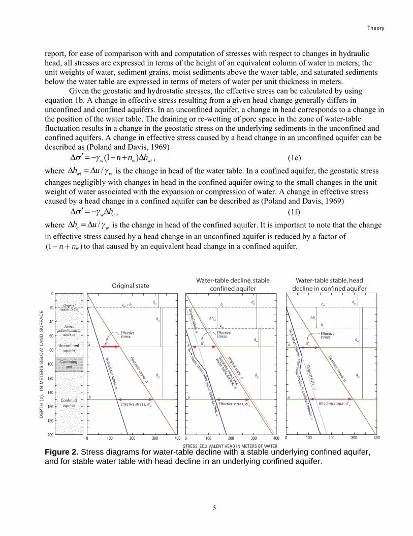
report, for ease of comparison with and computation of stresses with respect to changes in hydraulic head, all stresses are expressed in terms of the height of an equivalent column of water in meters; the unit weights of water, sediment grains, moist sediments above the water table, and saturated sediments below the water table are expressed in terms of meters of water per unit thickness in meters. Given the geostatic and hydrostatic stresses, the effective stress can be calculated by using equation 1b. A change in effective stress resulting from a given head change generally differs in unconfined and confined aquifers. In an unconfined aquifer, a change in head corresponds to a change in the position of the water table. The draining or re-wetting of pore space in the zone of water-table fluctuation results in a change in the geostatic stress on the underlying sediments in the unconfined and confined aquifers. A change in effective stress caused by a head change in an unconfined aquifer can be described as (Poland and Davis, 1969) , (1e) (1 )w wn n hσ γ′Δ = − − + Δ wt
w
Figure 2. Stress diagrams for water-table decline with a stable underlying confined aquifer, nd for stable water table with head decline in an underlying confined aquifer.
where is the change in head of the water table. In a confined aquifer, the geostatic stress changes negligibly with changes in head in the confined aquifer owing to the small changes in the unit weight of water associated with the expansion or compression of water. A change in effective stress caused by a head change in a confined aquifer can be described as (Poland and Davis, 1969)
/wt wh u γΔ = Δ
, (1f) w chσ γ′Δ = − Δwhere is the change in head of the confined aquifer. It is important to note that the change in effective stress caused by a head change in an unconfined aquifer is reduced by a factor of
to that caused by an equivalent head change in a confined aquifer.
/ch u γΔ = Δ
)wn n− +(1
a
’a
4000 300200
STRESS, EQUIVALENT HEAD IN METERS OF WATER
DEPTH
(z)
, IN
METER
S B
ELO
W L
AN
D S
UR
FAC
E
100200
180
160
140
120
100
80
60
40
20
0
Confiningunit
Confinedaquifer
Unconfinedaquifer
Originalwater table
Activepotentiometric
surface
Hydrostatic stress, u
Geostatic stress,
Effectivestress
Effective stress, ’b
dm dmzwt = hc
dsa
dsb
’a
4000 300200100
Hydrostatic stress after water-table
decline, u
Effectivestress
Effective stress, ’b Effective stress, ’b
hc
hc
dm
zwt
dsa
dsb
dsa
dsb
hwt
Original stateWater-table decline, stable
confined aquiferWater-table stable, head
decline in confined aquifer
a
b b
a
b
a
4000 300200100
Geostatic stress,
Effectivestress
zwt
Original state, u Hydrostatic stressafterhead
decline inconfined aquifer, u
’a
hc
Geostatic stress after
water-table decline,
Original state, u
Original state,
5
User Guide to the Subsidence and Aquifer-System Compaction Package (SUB-WT) for Water-Table Aquifers
changes in these stresses caused by the lowering of hydraulic heads in an idealized unconfined aquiferThe stresses for the idealized aquifer system are computed by using the specified value
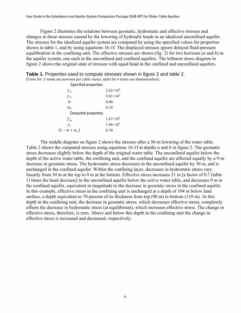
Figure 2 illustrates the relations between geostatic, hydrostatic and effective stresses and .
s for properties ure
shown in table 1, and by using equations 1b-1f. The displayed stresses ignore delayed fluid-pressequilibration in the confining unit. The effective stresses are shown (fig. 2) for two horizons (a and b) inthe aquifer system, one each in the unconfined and confined aquifers. The leftmost stress diagram in figure 2 shows the original state of stresses with equal head in the confined and unconfined aquifers.
Table 1. Properties used to compute stresses shown in figure 2 and table 2. [Units for γ terms are newtons per cubic meter; units for n terms are dimensionless]
Specified properties
gγ 2.62×10⁴ 3
wγ 9.81×10n 0.40
puted properties10
wnCom
0.10
mγ 1.67× 4
sγ 1.96×10⁴
0.70
The middle diagram on figure 2 shows the stresses after a 30-m lowering of the water table. Table 2 shows the computed stresses using equations 1b-1f at depths a and b in figure 2. The geostatic
ress decreases slightly below the depth of the original water table. The unconfined aquifer below the epth o 9-m
(1 )wn+ n−
std f the active water table, the confining unit, and the confined aquifer are affected equally by a decrease in geostatic stress. The hydrostatic stress decreases in the unconfined aquifer by 30 m, and is unchanged in the confined aquifer. Within the confining layer, decreases in hydrostatic stress vary linearly from 30 m at the top to 0 m at the bottom. Effective stress increases 21 m [a factor of 0.7 (table 1) times the head decrease] in the unconfined aquifer below the active water table, and decreases 9 m in the confined aquifer, equivalent in magnitude to the decrease in geostatic stress in the confined aquifer.In this example, effective stress in the confining unit is unchanged at a depth of 104 m below land surface, a depth equivalent to 70 percent of its thickness from top (90 m) to bottom (110 m). At this depth in the confining unit, the decrease in geostatic stress, which decreases effective stress, completely offsets the decrease in hydrostatic stress (at equilibrium), which increases effective stress. The change in effective stress, therefore, is zero. Above and below this depth in the confining unit the change in effective stress is increased and decreased, respectively.
6
Theory
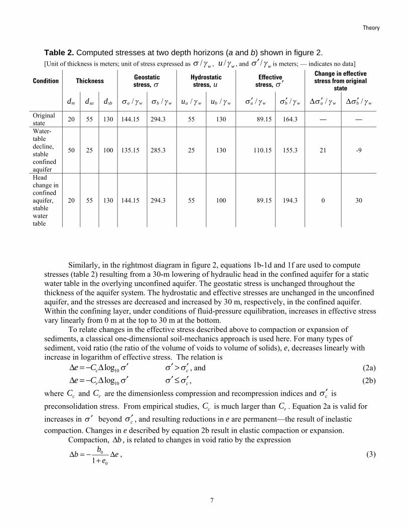
Table 2. Computed stresses at two depth horizons (a and b) shown in figure 2. [Unit of thickness is meters; unit of stress expressed as , , and is meters; — indicates no data] / wσ γ / wu γ / wσ γ′
Condition Thickness Geostatic stress, σ
Hydrostatic stress, u
Effective stress, σ ′
Change in effective stress from original
state
md sad sbd /a wσ γ /b wσ γ /a wu γ /b wu γ /a wσ γ′ /b wσ γ′ /a wσ γ′Δ /b wσ γ′Δ
Original state 20 55 130 144.15 294.3 55 130 89.15 164.3 — —
Water-table decline, stable confined aquifer
50 25 100 135.15 285.3 25 130 110.15 155.3 21 -9
Head change in confined aquifer, stable water table
20 55 130 144.15 294.3 55 100 89.15 194.3 0 30
Similarly, in the rightmost diagram in figure 2, equations 1b-1d and 1f are used to compute stresses (table 2) resulting from a 30-m lowering of hydraulic head in the confined aquifer for a static water table in the overlying unconfined aquifer. The geostatic stress is unchanged throughout the thickness of the aquifer system. The hydrostatic and effective stresses are unchanged in the unconfined aquifer, and the stresses are decreased and increased by 30 m, respectively, in the confined aquifer. Within the confining layer, under conditions of fluid-pressure equilibration, increases in effective stress vary linearly from 0 m at the top to 30 m at the bottom.
To relate changes in the effective stress described above to compaction or expansion of sediments, a classical one-dimensional soil-mechanics approach is used here. For many types of sediment, void ratio (the ratio of the volume of voids to volume of solids), e, decreases linearly with increase in logarithm of effective stress. The relation is
10logce CΔ = − Δ
10logre C σ ′Δ = − Δσ ′ σ σ′ ′
′σ ′
′
bΔ
, and (2a) c>
cσ σ′ ≤ , (2b) where and are the dimensionless compression and recompression indices and is preconsolidation stress. From empirical studies, is much larger than . Equation 2a is valid for increases in σ beyond σ , and resulting reductions in e are permanent—the result of inelastic compaction. Changes in e described by equation 2b result in elastic compaction or expansion.
cC rC c
cC rC′ c
Compaction, , is related to changes in void ratio by the expression 0
01b
eΔ = − b e
+Δ , (3)
7

User Guide to the Subsidence and Aquifer-System Compaction Package (SUB-WT) for Water-Table Aquifers
8
σ′ ′
where is initial thickness and is initial void ratio. The sign convention for , as used in this report is positive for compaction and negative for expansion. Inelastic compaction, , and elastic compaction, , can be computed by combining equations 2 and 3 and using the relation
. Those expressions are
0b
10
0e bΔ
ibΔ
ebΔ0.434σ ′log /σΔ = Δ
( )0
0
0.4341
ci
b Cbe
σσ
′ΔΔ =′+
, and (4a)
( )0
0
0.4341
re
b Cbe
σσ
′ΔΔ =′+
. (4b)
According to Leake and Prudic (1991), and are related to by ibΔ ebΔ σ ′Δ
0skvi
w
S bb σγ
′Δ = Δ , and (5a)
0skee
w
S bb σγ
′Δ = Δ , (5b)
where skvS and skeS are inelastic (virgin) and elastic skeletal specific-storage values, respectively. Equations 4 and 5 imply that skvS and skeS can be expressed as
( )0
0.4341
c wskv
CSeγ
σ=
′ +, and (6a)
( )0
0.4341
r wske
CSeγ
σ=
′ +. (6b)
Equation 6a is consistent with expressions given by Helm (1976), Jorgensen (1980), and Neuman and others (1982). Note that skeletal specific storage is inversely related to effective stress. For deep sediments, σ will be large, and reductions in u resulting from ground-water pumping are not likely to make large percentage changes in σ . For that case,
′′ skvS and skeS can be treated as constants with little
resulting error. On the other hand, for shallow sediments where σ is relatively small, changes in u could result in relatively large percentage changes in σ .
′′
Equations 4a and 4b can be combined into a general expression for compaction or expansion of sediments, , between times and as follows: bΔ 1nt − nt
( ) ( ) (0, 1 , 1 1
0
0.4341 n n c n r c n n
bb C Ce
σ σ σ σσ − −⎡ )−′ ′ ′ ′Δ = − + −⎣′+
1
⎤⎦, 1
, 1
,,
c n c nn
r n c n
CC
Cσ σσ σ
−
−
′ ′>⎧= ⎨ ′ ′≤⎩
, (7)
where and are effective-stress values at times and , respectively, and is the
preconsolidation-stress value at time . Note that the relation of to is used to determine
whether the value of is or . The expression gives correct results for overly consolidated sediments, for normally consolidated sediments, and for sediments in transition from overconsolidation to normal consolidation.
1nσ −′ nσ ′ 1nt − nt ,c nσ −′
1nt −
r
nσ ′ , 1c nσ −′
nC cC C

Incorporating Interbed Storage into the Ground-Water Flow Equations
Incorporating Interbed Storage into the Ground-Water Flow Equations
The ground-water flow model (MODFLOW) by Harbaugh and others (2000) and Harbaugh (2005) is a modular computer program designed to allow addition of simulation capabilities without extensive modification of the existing program. Hoffmann and others (2003) documented the SUB Package for MODFLOW for simulating aquifer-system compaction and land subsidence. A fundamental assumption of the SUB Package is that a decrease in head in an aquifer results in an equal increase in effective stress, σ . In water-table (unconfined) aquifers, a change in head changes both pore pressure, , and geostatic stress, σ , and a change in head does not produce an equal but opposite change in effective stress. Leake (1991, 1992) developed the Interbed Storage Package version 3 (IBS3) for MODFLOW to better simulate aquifer-system compaction in aquifers in which geostatic stress can vary. For this study, the IBS3 Package has been modified and updated as the Subsidence and Aquifer-System Package (SUB-WT) for water tables for use with MODFLOW-2000 (Harbaugh and others, 2000) and MODFLOW-2005 (Harbaugh, 2005).
′u
The MODFLOW program solves a form of the three-dimensional ground-water flow equation
xx yy zz sh h hK K K W hS
x x y y z z⎛ ⎞∂ ∂ ∂ ∂ ∂ ∂⎛ ⎞ ⎛ ⎞+ + − =⎜ ⎟⎜ ⎟ ⎜ ⎟∂ ∂ ∂ ∂ ∂ ∂⎝ ⎠ ⎝ ⎠ t
∂∂⎝ ⎠
, (8)
where x, y, and z are cartesian coordinates, aligned along the major axes of the hydraulic-conductivity tensor;
xxK , , and are principal components of the hydraulic-conductivity tensor; yyK zzKh is hydraulic head; W is volumetric flux per unit volume of sources and (or) sinks of water;
sS is specific storage of the aquifer; and t is time.
To treat sS as a scalar implicitly requires skeletal compressibility to be isotropic (Helm, 1987). In MODFLOW, equation 8 is approximated with finite differences. The finite-difference equations are written in terms of volumetric flow rather than flow per unit volume. For model cells with a water table, values of horizontal hydraulic conductivity are multiplied by head so that the product, transmissivity, is a function of saturated thickness. Also for water-table cells, the specific yield of the aquifer is used in the storage term on the right side. As such, the storage term in the finite-difference equation approximates the rate of flow to or from storage at the water table.
To simulate compaction and storage changes in MODFLOW, an expression is added to the finite-difference equations to account for the resulting rate of flow into or out of the compressible interbeds. The expression to be added to MODFLOW is derived from equation 7; however, because MODFLOW uses hydraulic head as a dependent variable, equation 7 must be rewritten. This is accomplished by using the Terzaghi relation (eq. 1b) . For cell , pore pressure, , can be expressed as
, where is total head and is elevation head. Substituting these two relations into equation 7 yields
n nu( )n n nu h z γ= − w nh nz
( ), 1 , 10 1
0 1
0.4341
c n c nw n nn n r
n w w w w
bb C h z Ce
σ σγ σ σσ γ γ γ γ
− − −
−
′ ′⎡ ⎤⎛ ⎞ ⎛ ′Δ = − + − + −⎢ ⎜ ⎟ ⎜′+ ⎝ ⎠ ⎝⎣ ⎦
⎞⎥⎟
⎠. (9)
9

User Guide to the Subsidence and Aquifer-System Compaction Package (SUB-WT) for Water-Table Aquifers
Note that geostatic stress, , is a variable in this equation. In an unconfined aquifer, varies as a function of the position of the water table, which commonly is assumed to equal the head. Equation 9 is further modified to express the rate of flow into or out of interbeds. This modification is accomplished by multiplying by the area of the finite-difference cell,
nσ nσ
A ; dividing by the model time step, ; and rearranging the resulting expression as follows:
ntΔ
, 1 , 1 1c n c nn n ni sk n n ske
n w w w w
AbQ S h z St
σ σσ σγ
⎤⎞′⎥⎟
⎠
, 1
, 1
,,γ γ γ
− − −′ ′⎡ ⎛ ⎞ ⎛′
= − + − + −⎢ ⎜ ⎟ ⎜Δ ⎝ ⎠ ⎝⎣ ⎦ skv n c n
skske n c n
SS
Sσ σσ σ
−
−
′ ′>⎧= ⎨ ′ ′≤⎩
, (10a)
( )1 0
0.4341
c wskv
n
CSeγ
σ −
=′ +
, and (10b)
( )1 0
0.4341
r wske
n
CSeγ
σ −
=′ +
, (10c)
where
iQ is the volumetric rate of flow to or from compressible interbeds,
ntΔ is , and 1n nt t −−
nz is the average elevation of interbeds in the layer at time . ntNote that all stress quantities in equations 9 and 10 are divided by . This operation has the effect of converting stress to an equivalent height of a column of water—head. For simplicity, the SUB-WT Package makes all calculations by using stress values expressed as head. Simulation of storage changes using equation 10 assumes that head changes in the coarse-grained aquifer material propagate through the fine-grained interbeds within each model time step. This assumption means that the method will work best for relatively thin, compressible interbeds. For relatively thick, extensive confining units, the method can be applied by simulating each confining unit as one or more separate model layers. For further discussion of the effects of delay in release of water from compressible interbeds, see Leake (1990) and Hoffmann and others (2003).
wγ
Thickness of Interbeds
In equation 10, the thickness term, , represents the total thickness of interbeds in a finite-difference cell at time nt . In an unconfined aquifer, thickness of compressible interbeds can change because of (1) compaction or expansion of individual interbeds and (2) changes in the position of the water table. Thickness changes from the first mechanism need not be considered because the ratio
remains constant even though and vary as sediments compact or expand. The values of and for interbeds in the saturated flow system can be held constant.
nb
/(1 )b +b e
e b e
Thickness changes from the second mechanism are addressed in the SUB-WT Package with an option that varies the thickness of interbeds in proportion to changes in saturated thickness of an unconfined model layer. This treatment of thickness is analogous to varying transmissivity in response to changes in saturated thickness. If this option is selected, the thickness used in the calculations is limited to the proportion of the total interbed thickness in the saturated interval. The values of thickness read into the SUB-WT Package, therefore, should be total thicknesses of compressible interbeds
10

Incorporating Interbed Storage into the Ground-Water Flow Equations
between the top and bottom of the model layer to which the system is assigned. For example, the total thickness for the upper aquifer shown in figure 1A would include interbeds in the saturated zone as was in the unsaturated zone. Because the thickness at time nt is used, the term in the finite-difference equations that includes thickness must be updated for each iteration. An assumption of this optiinterbeds are distributed uniformly throughout the thickness of the model layer so that a given percentage change in saturated thickness results in an equivalent percentage change in thickness of interbeds in the saturated interval. Another assumption is that interbeds above the water table do nsupply any water to the saturated flow system. Helm (1984) presented an approach to simulating continued compaction of fine-grained interbeds left behind by a declining water table. If the option vary thickness in proportion to saturated thickness is not used, the
ell
on is that
ot
to package uses the entire interbed
ickness specified to compute storage changes and compaction.
Avera
e
be the
require update of the layer elevations in MODFLOW, which are used by many different packages.
GeostIn calculating geostatic s of head), the SUB-WT Package uses the relation
th
ge Elevation of Interbeds The average elevation of interbeds in a model layer is used in the calculation of effective stress,
1nσ −′ , in the denominator of equation 9. For this value, the SUB-WT Package computes effective stressfrom geostatic and hydrostatic stress at the center of the saturated thickness in a layer. This use of the center of the saturated thickness assumes that the interbeds are uniformly distributed across the entire thickness of the model layer, as defined by the top and bottom elevations read in the Discretization Fil(DIS) input of MODFLOW. Layer center (the center of the saturated interval in a layer) is computed from computed head and layer bottom elevations read into the DIS input. For layers that do not containa water table, the layer center is a fixed reference point. For layers that contain a water table, the layer center changes by half the amount of any change in the water table. The datum for elevation mustsame as that used in the model. The average elevation of interbeds is not adjusted for changes in elevation from compaction of sediments because such adjustments would
atic Stress stress (in term
0m m s s
wγ w
G d G dσσγ
= + + , (11)
here
t sediments over the distance, , between the top of layer
w 0σ / wγ is the geostatic stress above the top of layer 1;
mG is average specific gravity of mois md 1 and the water table (fig. 1); and sG is average specific gravity of saturated sediments over the distance, sd , between the water
is tion 11 can rived from
table and the bottom of the layer. If the top of layer 1 is land surface, then the term 0 / wσ γ will be zero. For the case in which 0 /σ γzero, equa be de equation 1c by dividing each term by wγ and by using the relations /m m wG γ γ= and /
w
s s wG γ γ= . Calculations of effective stress in the numerator of equation 10are for the bottom of the model layer, as discussed in the following section; therefore, geostatic stress used to compute these effective stress quantities also must be taken at the bottom of the model layer.
a
The calculation of geostatic stress used in calculation of effective stress in the denominator of equations
11

User Guide to the Subsidence and Aquifer-System Compaction Package (SUB-WT) for Water-Table Aquifers
10b and 10c, , is taken at the center of each layer. For these calculations of geostatic stress, 1nσ −′ sd in equation 11 extends from the water table to the layer center.
As the model iterates to compute head, the SUB-WT Package recomputes and md sd so that the final values are consistent with the water-table elevation at the end of the time step. At a fixed point in the saturated flow system, a unit decline in the water table results in a change in geostatic stress of
. m sG G−Arrays of geostatic stress above layer 1, specific gravity of moist sediments, and specific gravity
of saturated sediments must be read in. A single two-dimensional array is read for each of these three data sets. This approach assumes that values of specific gravity of saturated and moist sediments do not vary significantly in the vertical dimension.
Effective Stress Effective stress is not read in, but rather is computed for each active cell in the model grid,
whether or not that cell includes systems of interbeds. Effective stress and other stress quantities in the numerator of equation 10 are taken at the bottom of the layer, using values of head from the most current iteration. The value of effective stress in the denominator of equation 10, however, is taken at time and at the level of the center of the saturated thickness in a cell. This approach has the effect of explicitly selecting storage properties on the basis of conditions at the end of the previous time step. At the end of a time step, the SUB-WT Package uses the Terzaghi relation to update effective stress with currently calculated geostatic stress, head, and layer-center elevations.
1nt −
A change in position of a water table results in changes in effective-stress in all underlying model layers. For example, suppose that the head change in the upper unconfined layer is and the head change in a lower confined layer is . The corresponding changes in effective stress are and . The relations between change in head and change in effective stress are
wthΔ
chΔ a′σΔ
bσ ′Δ1
2a = − s
m wtw
GG hσγ
′Δ −⎛ ⎞− Δ⎜ ⎟⎝ ⎠, and (12a)
( )bm s wt
w
G G h hσγ
′Δc− Δ − Δ . (12b) = −
For typical values of mG and sG , equation 12a computes an effective-stress change larger than the head change, reflecting the changing position of the layer center. For the lower aquifer, the change in effective stress is dependent on head change in the upper and lower layers. For typical values of and
mG
sG with the same head changes in both layers, equation 12b computes an effective-stress change less than the head change.
Preconsolidation Stress Previous computer programs by Meyer and Carr (1979), Williamson and others (1989), Leake
and Prudic (1991), and Hoffmann and others (2003) assume preconsolidation stress is related to a preconsolidation head. The preconsolidation head is used to switch between elastic and inelastic storage properties— specific storage changes to inelastic values whenever the hydraulic head falls below the preconsolidation head. In contrast, the SUB-WT Package uses preconsolidation stress as an effective
12

Incorporating Interbed Storage into the Ground-Water Flow Equations
13
stress. T
tion stress is below the initial effective stress. The preconsolidation stress is changed to the effective stress at the end
el cells where the preconsolidation stress has been exceeded.
option is availabl ad in either (A) inmpressio sed to compute the
ultiplied to ed for equation 10.
s in the lues are read in for each cell in each system of
interbeds at the start of a simulation. As outlined in the previous section, the values are used in computing constant parts of coefficients in equation 10.
his approach is taken because for some model layers, a single head-change value is notsufficient to specify an effective-stress value (see equation 12b).
Initial preconsolidation stress can be defined in one of two ways. First, arrays of initial preconsolidation stress can be read into the SUB-WT Package for each model cell. Definition of an internally consistent distribution of initial preconsolidation stress over an entire model domain can bedifficult. For this reason, a second method of defining the distribution is provided. This method allows initial preconsolidation stress to be defined as an increment above initial effective stress at each cell. The computation is made by using an array of offset values for each cell and computed effective stressat each cell. Because preconsolidation stress is always greater than or equal to effective stress, initial values are changed to equal the initial effective stress for cells at which the preconsolida
of each time step for mod
Storage Properties An e to re elastic and elastic skeletal specific storage, or (B)
reco n and compression index. For either option, the values read are uquantities and , which are saved. These constants are m00.434 /(1 )rAC e+
t each iteration00.434 /(1 )cAC e+
obtain coefficients needby 1/n w nb γ σ −′ a
Void Ratio As was previously stated, the ratio /(1 )b e+ is constant; therefore, b and e for interbed
saturated flow system can be held constant. Void-ratio va

User Guide to the Subsidence and Aquifer-System Compaction Package (SUB-WT) for Water-Table Aquifers
Package Output
Flow quantities into and out of interbeds computed in the SUB-WT Package are added to the overall volumetric budget printed by MODFLOW. This printed budget includes flow rates and total volumes of water for all flow-component and stress packages used in a simulation. A single component, “INTERBED STORAGE,” is added for the SUB-WT Package. This component describes the changes in storage in all systems of interbeds. This component is equivalent to the storage terms calculated in the SUB Package (Hoffmann and others, 2003). The sign convention for storage changes in interbeds is the same as that used in other MODFLOW packages, with positive numbers for flow into the aquifer system and negative numbers for flow out of the aquifer system. Release of water from the interbeds is considered inflow to the aquifer system; uptake of water by the interbeds from the surrounding aquifers is considered outflow from the aquifer system.
During the execution of MODFLOW, the SUB-WT Package generates information related to interbeds, including information on subsidence, compaction, vertical displacement, system stresses, and other information. The package allows control of printing and saving this information. The SUB-WT Package Output Control should not be confused with the MODFLOW Output Control. These are two separate sets of instructions controlling different types of model output.
Thirteen types of arrays can be printed or saved for specified sets of time steps. Variable names for formats, unit numbers, and flags, and array identifiers for these output items are given in table 3. Specific definitions for these output items are as follows: 1. Subsidence: This quantity is the sum of the compaction from all interbed systems. In the printout or
header record of the saved array, the layer number for subsidence is set to 1. The sign convention for subsidence is positive for lowering and negative for uplift.
2. Compaction by model layer: The output option of compaction by model layer is the sum of compaction of all interbed systems within each model layer. The sign convention for compaction is positive for compression or shortening and negative for expansion. Arrays for model layers that do not contain any compressible interbeds are not printed or saved. The model-layer number is included in the printout or header records of the saved arrays.
3. Compaction by interbed system: This output option saves compaction for each interbed system. The sign convention for compaction is positive for compression or shortening and negative for expansion. The SUB-WT Package computes compaction for each system of interbeds. The model-layer numbers to which each system belongs are specified in array LNWT. Each model layer can include more than one system of interbeds. For printed arrays, the standard MODFLOW header indicates the model-layer number that includes the system and a line of text indicating the sequence number of the system preceding that record. For saved arrays, the header record includes the sequence number of the system in the field normally used for the layer number. The sequence number is derived from the order in which systems of interbeds are specified in the input data set.
4. Vertical displacement by model layer: Vertical displacement for a model layer is defined as the sum of the compaction in the layer and in all underlying layers. This displacement corresponds to movement of the upper surface of the model layer. The sign convention for vertical displacement is positive for lowering and negative for uplift. The vertical displacement for layer 1 is equal to the subsidence. Any layers below the lowest system of compressible interbeds will have zero vertical displacement. The model-layer number is included in the printout or header records of the saved arrays.
14
Package Output
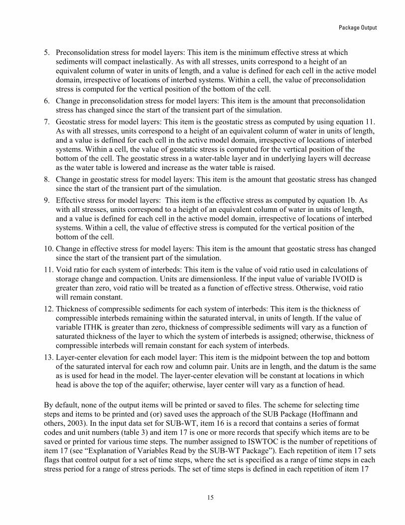
5. Preconsolidation stress for model layers: This item is the minimum effective stress at which sediments will compact inelastically. As with all stresses, units correspond to a height of an equivalent column of water in units of length, and a value is defined for each cell in the active model domain, irrespective of locations of interbed systems. Within a cell, the value of preconsolidation stress is computed for the vertical position of the bottom of the cell.
6. Change in preconsolidation stress for model layers: This item is the amount that preconsolidation stress has changed since the start of the transient part of the simulation.
7. Geostatic stress for model layers: This item is the geostatic stress as computed by using equation 11. As with all stresses, units correspond to a height of an equivalent column of water in units of length, and a value is defined for each cell in the active model domain, irrespective of locations of interbed systems. Within a cell, the value of geostatic stress is computed for the vertical position of the bottom of the cell. The geostatic stress in a water-table layer and in underlying layers will decrease as the water table is lowered and increase as the water table is raised.
8. Change in geostatic stress for model layers: This item is the amount that geostatic stress has changed since the start of the transient part of the simulation.
9. Effective stress for model layers: This item is the effective stress as computed by equation 1b. As with all stresses, units correspond to a height of an equivalent column of water in units of length, and a value is defined for each cell in the active model domain, irrespective of locations of interbed systems. Within a cell, the value of effective stress is computed for the vertical position of the bottom of the cell.
10. Change in effective stress for model layers: This item is the amount that geostatic stress has changed since the start of the transient part of the simulation.
11. Void ratio for each system of interbeds: This item is the value of void ratio used in calculations of storage change and compaction. Units are dimensionless. If the input value of variable IVOID is greater than zero, void ratio will be treated as a function of effective stress. Otherwise, void ratio will remain constant.
12. Thickness of compressible sediments for each system of interbeds: This item is the thickness of compressible interbeds remaining within the saturated interval, in units of length. If the value of variable ITHK is greater than zero, thickness of compressible sediments will vary as a function of saturated thickness of the layer to which the system of interbeds is assigned; otherwise, thickness of compressible interbeds will remain constant for each system of interbeds.
13. Layer-center elevation for each model layer: This item is the midpoint between the top and bottom of the saturated interval for each row and column pair. Units are in length, and the datum is the same as is used for head in the model. The layer-center elevation will be constant at locations in which head is above the top of the aquifer; otherwise, layer center will vary as a function of head.
By default, none of the output items will be printed or saved to files. The scheme for selecting time steps and items to be printed and (or) saved uses the approach of the SUB Package (Hoffmann and others, 2003). In the input data set for SUB-WT, item 16 is a record that contains a series of format codes and unit numbers (table 3) and item 17 is one or more records that specify which items are to be saved or printed for various time steps. The number assigned to ISWTOC is the number of repetitions of item 17 (see “Explanation of Variables Read by the SUB-WT Package”). Each repetition of item 17 sets flags that control output for a set of time steps, where the set is specified as a range of time steps in each stress period for a range of stress periods. The set of time steps is defined in each repetition of item 17
15
User Guide to the Subsidence and Aquifer-System Compaction Package (SUB-WT) for Water-Table Aquifers
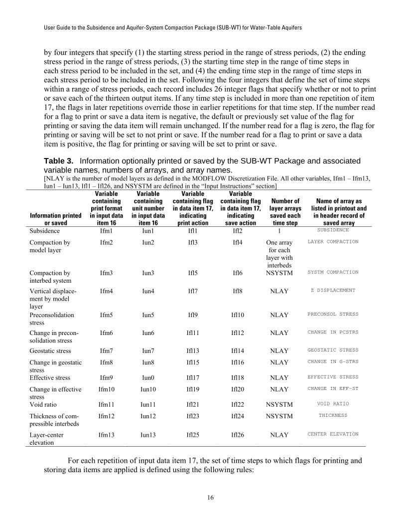
by four integers that specify (1) the starting stress period in the range of stress periods, (2) the ending stress period in the range of stress periods, (3) the starting time step in the range of time steps in each stress period to be included in the set, and (4) the ending time step in the range of time steps in each stress period to be included in the set. Following the four integers that define the set of time steps within a range of stress periods, each record includes 26 integer flags that specify whether or not to print or save each of the thirteen output items. If any time step is included in more than one repetition of item 17, the flags in later repetitions override those in earlier repetitions for that time step. If the number read for a flag to print or save a data item is negative, the default or previously set value of the flag for printing or saving the data item will remain unchanged. If the number read for a flag is zero, the flag for printing or saving will be set to not print or save. If the number read for a flag to print or save a data item is positive, the flag for printing or saving will be set to print or save.
Table 3. Information optionally printed or saved by the SUB-WT Package and associated variable names, numbers of arrays, and array names. [NLAY is the number of model layers as defined in the MODFLOW Discretization File. All other variables, Ifm1 – Ifm13, Iun1 – Iun13, Ifl1 – Ifl26, and NSYSTM are defined in the “Input Instructions” section]
Information printed or saved
Variable containing print format in input data
item 16
Variable containing
unit number in input data
item 16
Variable containing flag in data item 17,
indicating print action
Variable containing flag in data item 17,
indicating save action
Number of layer arrays saved each
time step
Name of array as listed in printout and in header record of
saved arraySubsidence Ifm1 Iun1 Ifl1 Ifl2 1 SUBSIDENCE
Compaction by model layer
Ifm2 Iun2 Ifl3 Ifl4 One array for each
layer with interbeds
LAYER COMPACTION
Compaction by interbed system
Ifm3 Iun3 Ifl5 Ifl6 NSYSTM SYSTM COMPACTION
Vertical displace- ment by model layer
Ifm4 Iun4 Ifl7 Ifl8 NLAY Z DISPLACEMENT
Preconsolidation stress
Ifm5 Iun5 Ifl9 Ifl10 NLAY PRECONSOL STRESS
Change in precon- solidation stress
Ifm6 Iun6 Ifl11 Ifl12 NLAY CHANGE IN PCSTRS
Geostatic stress Ifm7 Iun7 Ifl13 Ifl14 NLAY GEOSTATIC STRESS
Change in geostatic stress
Ifm8 Iun8 Ifl15 Ifl16 NLAY CHANGE IN G-STRS
Effective stress Ifm9 Iun0 Ifl17 Ifl18 NLAY EFFECTIVE STRESS
Change in effective stress
Ifm10 Iun10 Ifl19 Ifl20 NLAY CHANGE IN EFF-ST
Void ratio Ifm11 Iun11 Ifl21 Ifl22 NSYSTM VOID RATIO
Thickness of com-pressible interbeds
Ifm12 Iun12 Ifl23 Ifl24 NSYSTM THICKNESS
Layer-center elevation
Ifm13 Iun13 Ifl25 Ifl26 NLAY CENTER ELEVATION
For each repetition of input data item 17, the set of time steps to which flags for printing and
storing data items are applied is defined using the following rules:
16

Package Output
1. Any starting or ending stress period or time step that is specified to be less than 1 will be reset to 1.
2. Any starting or ending stress period that is specified to be greater than the total number of stress periods in the simulation (NPER) will be reset to NPER.
3. Any starting or ending time step that is specified to be greater than the total number of time steps in a particular stress period [NSTP(N) for stress period N] will be reset to NSTP(N).
4. Any ending stress period that is specified to be less than the corresponding starting stress period will be reset to the starting stress period.
5. Any ending time step that is specified to be less than the corresponding starting time step will be reset to the starting time step.
6. For the resulting range of stress periods, each time step within the resulting range of time steps will have the flags for printing or saving set as specified. The following example, described in more detail later in the section “Example simulation,” will
help in understanding this system. The simulation includes one steady-state stress period with one time step followed by two transient stress periods, each with 60 time steps. The desired output is (A) print subsidence, compaction by layer, preconsolidation stress, change in preconsolidation stress, geostatic stress, change in geostatic stress, effective stress, and change in effective stress for the last time step in stress period 2 and the last time step in stress period 3; and (B) save subsidence, compaction by layer, preconsolidation stress, geostatic stress, and effective stress to files. This output can be accomplished with the three records shown in figure 3. The first record (item 16 in input instructions) is an alternating series of formats for printing, and unit numbers for saving data items. The second record is a repetition of data item 17 that accomplishes the output listed in (A) and the second item is another repetition of data item 17 that accomplishes the output listed in (B).
Figure 3. Series of three records needed to specify output for an example simulation using the SUB-WT Package.
Note that the range of time steps in record 2 for stress periods 2 and 3 will be reset to go from 60 to 60 because the number read in, 100, is greater than the maximum number of time steps in each stress
17

User Guide to the Subsidence and Aquifer-System Compaction Package (SUB-WT) for Water-Table Aquifers
18
period. This accomplishes the action desired for the last time step in each period. Similarly, the range in time steps in the last record will be reset to go from 1 to 60, thereby resulting in the desired output for each time step in stress periods 2 and 3.
In addition to the output items specified above, the SUB-WT Package can save cell-by-cell flow terms to files in the manner that similar terms are saved for other flow-related packages. Terms are written to a file associated with the unit number specified by variable ISWTCB (see “Explanation of Variables Read by the SUB-WT Package”) for time steps when “SAVE BUDGET” or a non-zero value of variable ICBCFL (flag for writing cell-by-cell flow data) is specified in the MODFLOW Output Control file (for example, Harbaugh and others, 2000, p. 52). Cell-by-cell terms for rates of storage change will be written using the name “INTERBED STORAGE” in the header record.

Input Instructions
Input Instructions Input for the SUB-WT Package is read from the file that has the type “SWT” in the name file. Optional variables are shown in brackets. All single-valued variables in data items 1, 3, 16, and 17, and layer assignments for systems of interbeds in data item 2 are read in free format. Data items 1, 2, 3, and 16 consist of, at most, one record. Two-dimensional arrays in data items 4–15 are read with MODFLOW utility array readers U2DREL. For instructions on use of array readers, refer to Harbaugh and others (2000) or Harbaugh (2005). FOR EACH SIMULATION 1. Data: ISWTCB ISWTOC NSYSTM ITHK IVOID ISTPCS ICRCC 2. LNWT(NSYSTM) (Enter NSYSTM integers separated by one or more spaces or by commas.) 3. IZCFL IZCFM IGLFL IGLFM IESTFL IESTFM IPCSFL IPCSFM ISTFL ISTFM 4. GL0(NCOL,NROW) U2DREL 5. SGM(NCOL,NROW) U2DREL 6. SGS(NCOL,NROW) U2DREL The arrays in data items 7–13 are read for each of NSYSTM systems of interbeds. Read all arrays for system 1 first, then all arrays for system 2, and so on for each system. 7. THICK(NCOL,NROW) U2DREL 8. Sse(NCOL,NROW) U2DREL if ICRCC≠0 9. Ssv(NCOL,NROW) U2DREL if ICRCC≠0 10. Cr(NCOL,NROW) U2DREL if ICRCC=0 11. Cc(NCOL,NROW) U2DREL if ICRCC=0 12. VOID(NCOL,NROW) U2DREL 13. SUB(NCOL,NROW) U2DREL Module: U2DREL The arrays in data items 14 and 15 are read for each of NLAY model layers. Depending on the value of ISTPCS, read item 14 or item 15 sequentially from layer 1 to layer NLAY. 14. [PCSOFF(NCOL,NROW)] U2DREL if ISTPCS ≠ 0 15. [PCS(NCOL,NROW)] U2DREL if ISTPCS = 0
19

User Guide to the Subsidence and Aquifer-System Compaction Package (SUB-WT) for Water-Table Aquifers
16. [Ifm1 Iun1 Ifm2 Iun2 Ifm3 Iun3 … Ifm13 Iun13] if ISWTOC > 0 (Data item 16 consists of one record with 26 integers separated by one or more spaces or by commas.) 17. [ISP1 ISP2 ITS1 ITS2 Ifl1 Ifl2 Ifl3 … Ifl26] if ISWTOC > 0 (Data item 17 consists of ISWTOC records with 30 integers separated by one or more spaces or by commas. See the section entitled “Package Output” for a detailed explanation of the use of data item 17.)
Explanation of Variables Read by the SUB-WT Package
ISWTCB is a flag and unit number.
If ISWTCB > 0, it is the unit number to which cell-by-cell flow terms will be written when “SAVE BUDGET” or a non-zero value for ICBCFL is specified in MODFLOW Output Control (for example, Harbaugh and others, 2000, p. 52–55).
If ISWTCB ≤ 0, cell-by-cell flow terms will not be recorded. ISWTOC is a flag and unit number.
If ISWTOC > 0, it is the number of repetitions of item 17 to be read, each repetition of which defines a set of times steps and associated flags for printing and saving subsidence, compaction by layer, compaction by interbed system, vertical displacement, preconsolidation stress, change in preconsolidation stress, geostatic stress, change in geostatic stress, effective stress, change in effective stress, void ratio, thickness of interbeds, and layer-center elevation.
If ISWTOC ≤ 0, subsidence, compaction, vertical displacement, preconsolidation stress, change in preconsolidation stress, geostatic stress, change in geostatic stress, effective stress, change in effective stress, void ratio, thickness of interbeds, and layer-center elevation will not be printed or saved.
NSYSTM is the number of systems of interbeds. ITHK is a flag to determine how thicknesses of compressible sediments vary in response to
changes in saturated thickness.
If ITHK ≤ 0, thickness of compressible sediments is constant.
If ITHK > 0, thickness of compressible sediments varies in response to changes in saturated thickness.
IVOID is a flag to determine how void ratios of compressible sediments vary in response to
changes in saturated thickness. 20

Input Instructions
If IVOID ≤ 0, void ratio will be treated as a constant.
If IVOID > 0, void ratio will be treated as a variable.
ISTPCS is a flag to determine how initial preconsolidation stress will be obtained.
If ISTPCS ≠ 0, an array of offset values will be read in for each model layer. The offset values will be added to the initial effective stress to get initial preconsolidation stress.
If ISTPCS = 0, an array with initial preconsolidation stress values will be read in.
ICRCC is a flag to determine how recompression and compression indices will be obtained.
If ICRCC ≠ 0, arrays of elastic specific storage and inelastic skeletal specific storage will be read for each system of interbeds. The recompression index and compression index will not be read.
If ICRCC = 0, arrays of recompression index and compression index will be read for
each system of interbeds. Elastic skeletal specific storage and inelastic skeletal specific storage will not be read.
LNWT is a one-dimensional array specifying the model-layer assignments for each system of
interbeds. The array has NSYSTM values. IZCFL is a flag to specify whether or not initial calculated values of layer-center elevation will
be printed.
If IZCFL > 0, array will be printed using format code specified by variable IZCFM.
If IZCFL ≤ 0, array will not be printed.
IZCFM is a code for the format in which layer-center elevation will be printed. Format codes for IZCFM, IGLFM, IESTFM, IPCSFM, ISTFM, Ifm1, Ifm2, Ifm3, … Ifm13 are as follows:
0 - (10G11.4) 7 - (20F5.0) 1 - (11G10.3) 8 - (20F5.1) 2 - (9G13.6) 9 - (20F5.2) 3 - (15F7.1) 10 - (20F5.3) 4 - (15F7.2) 11 - (20F5.4) 5 - (15F7.3) 12 - (10G11.4) 6 - (15F7.4)
IGLFL is a flag to specify whether or not initial calculated values of geostatic stress will be
printed.
If IGLFL > 0, array will be printed using format specified by variable IGLFM.
21

User Guide to the Subsidence and Aquifer-System Compaction Package (SUB-WT) for Water-Table Aquifers
If IGLFL ≤ 0, array will not be printed.
IGLFM is a code for the format in which geostatic stress will be printed. IESTFL is a flag to specify whether or not initial calculated values of effective stress will be
printed.
If IESTFL > 0, array will be printed using format specified by variable IESTFM.
If IESTFL ≤ 0, array will not be printed.
IESTFM is a code for the format in which effective stress will be printed. IPCSFL is a flag to specify whether or not initial calculated values of preconsolidation stress will
be printed.
If IPCSFL > 0, array will be printed using format specified by variable IPCSFM.
If IPCSFL ≤ 0, array will not be printed.
IPCSFM is a code for the format in which preconsolidation stress will be printed. ISTFL is a flag to specify whether or not initial equivalent storage properties will be printed for
each system of interbeds. If ICRCC≠0, the equivalent storage properties that can be printed are recompression and compression indices (Cr and Cc), which are calculated from elastic and inelastic skeletal specific storage (Sske and Sskv). If ICRCC=0, equivalent storage properties that can be printed are elastic and inelastic skeletal specific storage, which are calculated from the recompression and compression indices.
If ISTFL > 0, array will be printed using format specified by variable ISTFM.
If ISTFL ≤ 0, array will not be printed.
ISTFM is a code for the format in which equivalent storage properties will be printed. GL0 is an array specifying the geostatic stress above model layer 1. If the top of model layer 1
is the land surface, enter values of zero for this array. SGM is an array specifying the specific gravity of moist or unsaturated sediments. SGS is an array specifying the specific gravity of saturated sediments. THICK is an array specifying the thickness of compressible sediments. Sse is an array specifying the initial elastic skeletal specific storage of compressible beds. Ssv is an array specifying the initial inelastic skeletal specific storage of compressible beds.
22

Input Instructions
Cr is an array specifying the recompression index of compressible beds. Cc is an array specifying the compression index of compressible beds. VOID is an array specifying the initial void ratio of compressible beds. SUB is an array specifying the initial compaction in each system of interbeds. Compaction
values computed by the package are added to values in this array so that printed or stored values of compaction and land subsidence may include previous components. Values in this array do not affect calculations of storage changes or resulting compaction. For simulations in which output values will reflect compaction and subsidence since the start of the simulation, enter zero values for all elements of this array.
PCSOFF is an array specifying the offset from initial effective stress to initial preconsolidation
stress at the bottom of the model layer in units of height of a column of water. PCS is an array specifying the initial preconsolidation stress, in units of height of a column of
water, at the bottom of the model layer. Ifm1 is a code for the format in which subsidence will be printed. Format codes for variables
Ifm1, Ifm2, Ifm3, … Ifm13 are the same as those listed under variable IZCFM. Iun1 is the unit number to which subsidence will be written if it is saved on disk. Ifm2 is a code for the format in which compaction by layer will be printed. Iun2 is the unit number to which compaction by layer will be written if it is saved on disk. Ifm3 is a code for the format in which compaction by system will be printed. Iun3 is the unit number to which compaction by system will be written if it is saved on disk. Ifm4 is a code for the format in which vertical displacement will be printed. Iun4 is the unit number to which vertical displacement will be written if it is saved on disk. Ifm5 is a code for the format in which preconsolidation stress will be printed. Iun5 is the unit number to which preconsolidation stress will be written if it is saved on disk. Ifm6 is a code for the format in which change in preconsolidation stress will be printed. Iun6 is the unit number to which change in preconsolidation stress will be written if it is saved
on disk. Ifm7 is a code for the format in which geostatic stress will be printed.
23

User Guide to the Subsidence and Aquifer-System Compaction Package (SUB-WT) for Water-Table Aquifers
Iun7 is the unit number to which geostatic stress will be written if it is saved on disk. Ifm8 is a code for the format in which change in geostatic stress will be printed. Iun8 is the unit number to which change in geostatic stress will be written if it is saved on
disk. Ifm9 is a code for the format in which effective stress will be printed. Iun9 is the unit number to which effective stress will be written if it is saved on disk. Ifm10 is a code for the format in which change in effective stress will be printed. Iun10 is the unit number to which change in effective stress will be written if it is saved on
disk. Ifm11 is a code for the format in which void ratio will be printed. Iun11 is the unit number to which void ratio will be written if it is saved on disk. Ifm12 is a code for the format in which thickness of compressible sediments will be printed. Iun12 is the unit number to which thickness of compressible sediments will be written if it is
saved on disk. Ifm13 is a code for the format in which layer-center elevation will be printed. Iun13 is the unit number to which layer-center elevation will be written if it is saved on disk. The variables ISP1, ISP2, ITS1, ITS2, and Ifl1–Ifl26 are used to control printing and saving of information generated by the SUB-WT Package during program execution. The use of some of these variables is explained in more detail in the “Package Output” section. The default condition for flags Ifl1 through Ifl13 is to not print or save the indicated information. ISP1 is the starting stress period in the range of stress periods to which output flags Ifl1---Ifl26
apply. If the value of ISP1 is less than 1, the SUB-WT Package will change the number to 1.
ISP2 is the ending stress period in the range of stress periods and time steps to which output flags Ifl1---Ifl26 apply. If the value of ISP2 is greater than NPER (the number of stress periods in the simulation), the SUB-WT Package will change the number to NPER.
ITS1 is the starting time step in the range of time steps in each of the stress periods ISP1 through ISP2 to which output flags Ifl1 through Ifl26 apply. If the value of ITS1 is less than 1, the SUB-WT Package will change the number to 1.
ITS2 is the ending time step in the range of time steps in each of stress periods ISP1---ISP2 to which output flags Ifl1 through Ifl26 apply. If the value of ITS2 is greater than the
24

Input Instructions
number of time steps in a given stress period, the SUB-WT Package will change the number to the number of time steps in that stress period.
Ifl1 is the output flag for printing subsidence for the set of time steps specified by ISP1, ISP2,
ITS1, and ITS2. If Ifl1 < 0, use default or previously defined settings of Ifl1 for printing
subsidence. If Ifl1 = 0, do not print subsidence. If Ifl1 > 0, print subsidence.
Ifl2 is the output flag for saving subsidence to an unformatted disk file for the set of time
steps specified by ISP1, ISP2, ITS1, and ITS2. If Ifl2 < 0, use default or previously defined settings of Ifl2 for saving
subsidence. If Ifl2 = 0, do not save subsidence. If Ifl2 > 0, save subsidence.
Ifl3 is the output flag for printing compaction by layer for the set of time steps specified by
ISP1, ISP2, ITS1, and ITS2. If Ifl3 < 0, use default or previously defined settings of Ifl3 for printing
compaction by layer. If Ifl3 = 0, do not print compaction by layer. If Ifl3 > 0, print compaction by layer.
Ifl4 is the output flag for saving compaction by layer to an unformatted disk file for the set of
time steps specified by ISP1, ISP2, ITS1, and ITS2. If Ifl4 < 0, use default or previously defined settings of Ifl4 for saving
compaction by layer. If Ifl4 = 0, do not save compaction by layer. If Ifl4 > 0, save compaction by layer.
Ifl5 is the output flag for printing compaction by interbed system for the set of time steps
specified by ISP1, ISP2, ITS1, and ITS2. If Ifl5 < 0, use default or previously defined settings of Ifl5 for printing
compaction by interbed system. If Ifl5 = 0, do not print compaction by interbed system. If Ifl5 > 0, print compaction by interbed system.
Ifl6 is the output flag for saving compaction by interbed system to an unformatted disk file
for the set of time steps specified by ISP1, ISP2, ITS1, and ITS2. If Ifl6 < 0, use default or previously defined settings of Ifl6 for saving
compaction by interbed system. If Ifl6 = 0, do not save compaction by interbed system. If Ifl6 > 0, save compaction by interbed system.
Ifl7 is the output flag for printing vertical displacement for the set of time steps specified by
ISP1, ISP2, ITS1, and ITS2. If Ifl7 < 0, use default or previously defined settings of Ifl7 for printing vertical
displacement.
25

User Guide to the Subsidence and Aquifer-System Compaction Package (SUB-WT) for Water-Table Aquifers
If Ifl7 = 0, do not print vertical displacement. If Ifl7 > 0, print vertical displacement.
Ifl8 is the output flag for saving vertical displacement to an unformatted disk file for the set
of time steps specified by ISP1, ISP2, ITS1, and ITS2. If Ifl8 < 0, use default or previously defined settings of Ifl8 for saving vertical
displacement. If Ifl8 = 0, do not save vertical displacement. If Ifl8 > 0, save vertical displacement.
Ifl9 is the output flag for printing preconsolidation stress for the set of time steps specified by
ISP1, ISP2, ITS1, and ITS2. If Ifl9 < 0, use default or previously defined settings of Ifl9 for printing
preconsolidation stress. If Ifl9 = 0, do not print preconsolidation stress. If Ifl9 > 0, print preconsolidation stress.
Ifl10 is the output flag for saving preconsolidation stress to an unformatted disk file for the set
of time steps specified by ISP1, ISP2, ITS1, and ITS2. If Ifl10 < 0, use default or previously defined settings of Ifl10 for saving
preconsolidation stress. If Ifl10 = 0, do not save preconsolidation stress. If Ifl10 > 0, save preconsolidation stress.
Ifl11 is the output flag for printing change in preconsolidation stress for the set of time steps
specified by ISP1, ISP2, ITS1, and ITS2. If Ifl11 < 0, use default or previously defined settings of Ifl11 for printing change
in preconsolidation stress. If Ifl11 = 0, do not print change in preconsolidation stress. If Ifl11 > 0, print change in preconsolidation stress.
Ifl12 is the output flag for saving change in preconsolidation stress to an unformatted disk file
for the set of time steps specified by ISP1, ISP2, ITS1, and ITS2. If Ifl12 < 0, use default or previously defined settings of Ifl12 for saving change in
preconsolidation stress. If Ifl12 = 0, do not save change in preconsolidation stress. If Ifl12 > 0, save change in preconsolidation stress.
Ifl13 is the output flag for printing geostatic stress for the set of time steps specified by ISP1,
ISP2, ITS1, and ITS2. If Ifl13 < 0, use default or previously defined settings of Ifl13 for printing
geostatic stress. If Ifl13 = 0, do not print geostatic stress. If Ifl13 > 0, print geostatic stress.
Ifl14 is the output flag for saving geostatic stress to an unformatted disk file for the set of time
steps specified by ISP1, ISP2, ITS1, and ITS2. If Ifl14 < 0, use default or previously defined settings of Ifl14 for saving geostatic
stress.
26
Input Instructions
If Ifl14 = 0, do not save geostatic stress. If Ifl14 > 0, save geostatic stress.
Ifl15 is the output flag for printing change in geostatic stress for the set of time steps specified
by ISP1, ISP2, ITS1, and ITS2. If Ifl15 < 0, use default or previously defined settings of Ifl15 for printing change
in geostatic stress. If Ifl15 = 0, do not print change in geostatic stress. If Ifl15 > 0, print change in geostatic stress.
Ifl16 is the output flag for saving change in geostatic stress to an unformatted disk file for the
set of time steps specified by ISP1, ISP2, ITS1, and ITS2. If Ifl16 < 0, use default or previously defined settings of Ifl16 for saving change in
geostatic stress. If Ifl16 = 0, do not save change in geostatic stress. If Ifl16 > 0, save change in geostatic stress.
Ifl17 is the output flag for printing effective stress for the set of time steps specified by ISP1,
ISP2, ITS1, and ITS2. If Ifl17 < 0, use default or previously defined settings of Ifl17 for printing effective
stress. If Ifl17 = 0, do not print effective stress. If Ifl17 > 0, print effective stress.
Ifl18 is the output flag for saving effective stress to an unformatted disk file for the set of time
steps specified by ISP1, ISP2, ITS1, and ITS2. If Ifl18 < 0, use default or previously defined settings of Ifl18 for saving effective
stress. If Ifl18 = 0, do not save effective stress. If Ifl18 > 0, save effective stress.
Ifl19 is the output flag for printing change in effective stress for the set of time steps specified
by ISP1, ISP2, ITS1, and ITS2. If Ifl19 < 0, use default or previously defined settings of Ifl19 for printing change
in effective stress. If Ifl19 = 0, do not print change in effective stress. If Ifl19 > 0, print change in effective stress.
Ifl20 is the output flag for saving change in effective stress to an unformatted disk file for the
set of time steps specified by ISP1, ISP2, ITS1, and ITS2. If Ifl20 < 0, use default or previously defined settings of Ifl20 for saving change in
effective stress. If Ifl20 = 0, do not save change in effective stress. If Ifl20 > 0, save change in effective stress.
Ifl21 is the output flag for printing void ratio for the set of time steps specified by ISP1, ISP2,
ITS1, and ITS2. If Ifl21 < 0, use default or previously defined settings of Ifl21 for printing void
ratio.
27

User Guide to the Subsidence and Aquifer-System Compaction Package (SUB-WT) for Water-Table Aquifers
28
If Ifl21 = 0, do not print void ratio. If Ifl21 > 0, print void ratio.
Ifl22 is the output flag for saving void ratio to an unformatted disk file for the set of time steps
specified by ISP1, ISP2, ITS1, and ITS2. If Ifl22 < 0, use default or previously defined settings of Ifl22 for saving void
ratio. If Ifl22 = 0, do not save void ratio. If Ifl22 > 0, save void ratio.
Ifl23 is the output flag for printing compressible bed thickness for the set of time steps
specified by ISP1, ISP2, ITS1, and ITS2. If Ifl23 < 0, use default or previously defined settings of Ifl23 for printing
compressible bed thickness. If Ifl23 = 0, do not print compressible bed thickness. If Ifl23 > 0, print compressible bed thickness.
Ifl24 is the output flag for saving compressible bed thickness to an unformatted disk file for
the set of time steps specified by ISP1, ISP2, ITS1, and ITS2. If Ifl24 < 0, use default or previously defined settings of Ifl24 for saving
compressible bed thickness. If Ifl24 = 0, do not save compressible bed thickness. If Ifl24 > 0, save compressible bed thickness.
Ifl25 is the output flag for printing layer-center elevation for the set of time steps specified by
ISP1, ISP2, ITS1, and ITS2. If Ifl25 < 0, use default or previously defined settings of Ifl25 for printing layer-
center elevation. If Ifl25 = 0, do not print layer-center elevation. If Ifl25 > 0, print layer-center elevation.
Ifl26 is the output flag for saving layer-center elevation to an unformatted disk file for the set
of time steps specified by ISP1, ISP2, ITS1, and ITS2. If Ifl26 < 0, use default or previously defined settings of Ifl26 for saving layer-
center elevation. If Ifl26 = 0, do not save layer-center elevation. If Ifl26 > 0, save layer-center elevation.

Practical Considerations for Using the SUB-WT Package
Practical Considerations for Using the SUB-WT Package Users applying the SUB-WT Package may benefit from consideration of certain aspects of the
design of the package and MODFLOW. Some of the suggestions in the following sections are taken from the report documenting the SUB Package (Hoffmann and others, 2003), but also are applicable for simulations using the SUB-WT Package.
Compatibility of the SUB-WT Package with Versions of MODFLOW Several updated versions of the original MODFLOW (McDonald and Harbaugh, 1984) have
been released. These are referred to as MODFLOW-88 (McDonald and Harbaugh, 1988), MODFLOW-96 (Harbaugh and McDonald, 1996), MODFLOW-2000 (Harbaugh and others, 2000), and MODFLOW-2005 (Harbaugh, 2005). As of the release of this report, the SUB-WT Package is compatible only with MODFLOW-2000, and MODFLOW-2005, as is the SUB Package. Users of older versions of MODFLOW may use the Interbed Storage Package (Leake and Prudic, 1991) to simulate aquifer-system compaction.
Simulation of Flow in and Compaction of Confining Units Compressible sediments in aquifer systems may occur as discontinuous interbeds within
aquifers, or as extensive confining units adjacent to aquifers (fig. 1). In basin-scale ground-water models, simulation of flow and storage changes in individual discontinuous interbeds within aquifers is impractical because of difficulties in mapping the interbeds, and also because high-resolution finite-difference grids would be required to represent small geologic features. As was presented by Hoffmann and others (2003) this report documents an approach to simulating flow and storage changes in groups or systems of interbeds. Flow and storage changes in individual confining units, however, can be simulated in basin-scale flow models. To simulate flow and storage changes in confining units, one model layer (fig. 1B) or a number of model layers (Hoffmann and others, 2003, fig. 5C) must be used to represent each confining unit. Increasing the number of model layers increases the accuracy in simulating flow and storage changes but also increases computation and computer storage requirements (Leake and others, 1994). One system of interbeds should be used for each layer in a confining unit. For cells entirely within a confining unit, the corresponding value of the THICK array should be set to the layer thickness. If the simulation uses the Block-Centered Flow Package (Harbaugh and others, 2000), vertical leakance values that reflect confining-unit properties must be entered into the VCONT array for the model layer above the confining unit and for all layers within the confining unit. A general expression for the equivalent vertical leakance between layers and , , is k 1k + 1/ 2( / )v kK b +
1/ 21 1
2( / )/( ) /( )v k
k v k k v k
K bb K b K+
+ +
=+
, (13)
where is the thickness of model layer , and kb k ( )v kK is the vertical hydraulic conductivity of model layer . VCONT values for the layer above and layers within a confining unit should be computed by using equation 13. If the simulation uses the Layer-Property Flow Package (Harbaugh and others, 2000), vertical conductance terms are computed automatically using thickness values from layer-bottom elevations in the discretization file and vertical hydraulic conductivity values. Users should make sure that values of the LAYCBD array in the discretization file are set to 0 for layers in the vertical interval over which a confining unit is explicitly represented with model layers. (LAYCBD is a flag, with one value for each model layer that indicates whether or not a layer has a Quasi-3D confining unit below it.)
k
29

User Guide to the Subsidence and Aquifer-System Compaction Package (SUB-WT) for Water-Table Aquifers
30
Use of Steady-State Stress Periods in MODFLOW In MODFLOW-2000 and MODFLOW-2005, each stress period may be either steady-state or
transient. The ability to mix steady-state and transient stress periods in a single simulation allows users to set up an initial steady-state stress period that simulates predevelopment conditions and subsequent stress periods that simulate transient post-development conditions (see sample problem). The SUB-WT Package need not make any calculations in steady-state stress periods, but the heads calculated by the model for a steady-state stress period are relevant to calculations made by the package for subsequent transient stress periods. When steady-state and transient stress periods are mixed in a simulation, the SUB-WT Package operates in the following manner: 1. If any stress periods other than the first are steady-state, the SUB-WT Package prints a message in
the listing file and aborts the simulation. Simulations are allowed in which the first stress period is steady-state and subsequent stress periods are transient, or in which all stress periods are transient.
2. At the end of the steady-state stress period, SUB-WT calculates or recalculates layer-center elevations, geostatic stress, and effective stress, and resets preconsolidation stress at locations for which the calculated effective stress is greater than the initial preconsolidation stress, specified or calculated at the start of the simulation.
3. The calculated values of effective, preconsolidation, and geostatic stresses are saved in arrays for possible later use in determining changes in these quantities.
4. Calculated arrays including layer-center elevation, geostatic stress, effective stress, preconsolidation stress, and equivalent storage properties are printed in the listing file if flags are set.
5. Equivalent storage properties (recompression and compression indices or elastic and inelastic skeletal specific storages) are computed and printed if a flag is set.
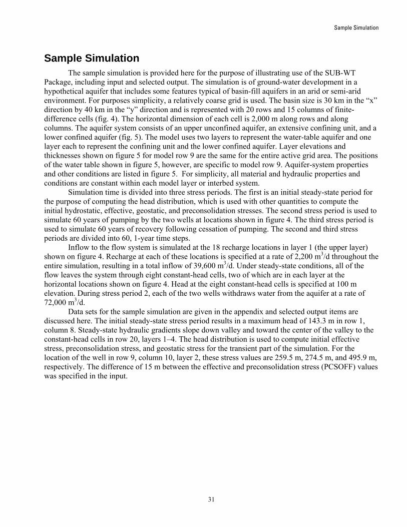
Sample Simulation
Sample Simulation The sample simulation is provided here for the purpose of illustrating use of the SUB-WT
Package, including input and selected output. The simulation is of ground-water development in a hypothetical aquifer that includes some features typical of basin-fill aquifers in an arid or semi-arid environment. For purposes simplicity, a relatively coarse grid is used. The basin size is 30 km in the “x” direction by 40 km in the “y” direction and is represented with 20 rows and 15 columns of finite-difference cells (fig. 4). The horizontal dimension of each cell is 2,000 m along rows and along columns. The aquifer system consists of an upper unconfined aquifer, an extensive confining unit, and a lower confined aquifer (fig. 5). The model uses two layers to represent the water-table aquifer and one layer each to represent the confining unit and the lower confined aquifer. Layer elevations and thicknesses shown on figure 5 for model row 9 are the same for the entire active grid area. The positions of the water table shown in figure 5, however, are specific to model row 9. Aquifer-system properties and other conditions are listed in figure 5. For simplicity, all material and hydraulic properties and conditions are constant within each model layer or interbed system.
Simulation time is divided into three stress periods. The first is an initial steady-state period for the purpose of computing the head distribution, which is used with other quantities to compute the initial hydrostatic, effective, geostatic, and preconsolidation stresses. The second stress period is used to simulate 60 years of pumping by the two wells at locations shown in figure 4. The third stress period is used to simulate 60 years of recovery following cessation of pumping. The second and third stress periods are divided into 60, 1-year time steps.
Inflow to the flow system is simulated at the 18 recharge locations in layer 1 (the upper layer) shown on figure 4. Recharge at each of these locations is specified at a rate of 2,200 m3/d throughout the entire simulation, resulting in a total inflow of 39,600 m3/d. Under steady-state conditions, all of the flow leaves the system through eight constant-head cells, two of which are in each layer at the horizontal locations shown on figure 4. Head at the eight constant-head cells is specified at 100 m elevation. During stress period 2, each of the two wells withdraws water from the aquifer at a rate of 72,000 m3/d.
Data sets for the sample simulation are given in the appendix and selected output items are discussed here. The initial steady-state stress period results in a maximum head of 143.3 m in row 1, column 8. Steady-state hydraulic gradients slope down valley and toward the center of the valley to the constant-head cells in row 20, layers 1–4. The head distribution is used to compute initial effective stress, preconsolidation stress, and geostatic stress for the transient part of the simulation. For the location of the well in row 9, column 10, layer 2, these stress values are 259.5 m, 274.5 m, and 495.9 m, respectively. The difference of 15 m between the effective and preconsolidation stress (PCSOFF) values was specified in the input.
31

User Guide to the Subsidence and Aquifer-System Compaction Package (SUB-WT) for Water-Table Aquifers
1
2
3
4
5
6
7
8
9
10
11
12
13
14
15
16
17
18
19
20
1 2 3 4 5 6 7 8 9 10 11 12 13 14 15MODEL COLUMN
MO
DE
L R
OW
Constant-head cells, layers 1-4Head is set to 100 meters above datum
Inactive area,layers 1-4
Inactive area,layers 1-4
Inactive area,layers 1-4
Inactive area,layers 1-4
Well, layer 2
Well, layer 4
Recharge cells, layer 1Inflow rate is 2,200cubic meters per day ateach recharge cell
Active area,layers 1-4
0 4 8 KILOMETERS
0 2 4 MILES1 3
2 6
Figure 4. Plan view of model domain showing active and inactive areas, and locations of recharge cells, constant-head cells, and wells.
32

Sample Simulation
Well
-350
-300
-250
-200
-150
-100
-50
0
50
100
150
0 5,000 10,000 15,000 20,000 25,000 30,000DISTANCE ALONG MODEL ROW 9, IN METERS
ELE
VA
TIO
N,I
NM
ETE
RS
Land surface (top of model and top of layer 1)
Layer 1— Upper part of water-table aquifer including fine-grained interbeds
Layer 4— Confined aquiferincluding fine-grainedinterbeds
Layer 3—Compressible fine-grained confining unit,
Properties and conditions represented in the SUB-WT Package:1. Interbed systems 1–4 are in layers 1–4 respectively2. Specific gravity of moist sediments is 1.7 and of saturated sediments is 2.03. Thicknesses of compressible sediments in systems 1–4 is 45, 70, 50, and 90 meters, respectively4. Recompression index for all systems of interbeds is 0.015. Compression index for all systems of interbeds is 0.256. Void ratio for all systems of interbeds is 0.827. Starting preconsolidation stress is 15 meters above starting effective stress for all active cellsProperties and conditions represented in the Layer-Property Flow Package:8. Horizontal hydraulic conductivity for layers 1–4 is 4, 4, 0.01, and 4 meters per day, respectively9. Vertical hydraulic conductivity for layers 1–4 is 0.4, 0.4, 0.01, and 0.4 meters per day, respectively10. Specific yield for layer 1 is 0.311. Specific storage from compressibility of water for layers 1–4 is 1×10⁻⁶ per meter
Initial water tableWater table after stress period 2
Layer 2— Lower part of water-table aquifer including fine-grained interbeds
z
x
Figure 5. Generalized section along model row 9 showing types of fine-grained sediments, model layering, and properties and conditions used in the example simulation. Aquifer-system properties and other conditions are listed in figure 5. For simplicity, all material and hydraulic properties and conditions are constant within each model layer or interbed system.
As specified in the input, equivalent skeletal specific storage values were calculated from recompression and compression indices and the initial effective stress distribution. Computed values of
33
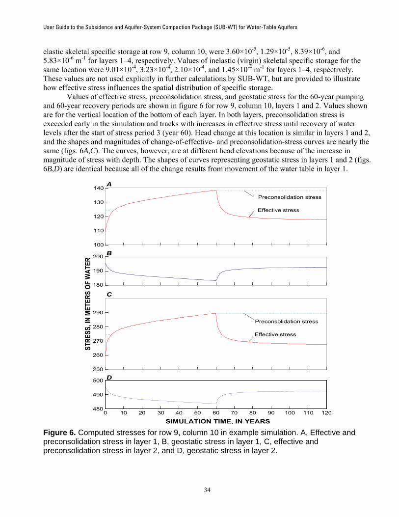
User Guide to the Subsidence and Aquifer-System Compaction Package (SUB-WT) for Water-Table Aquifers
elastic skeletal specific storage at row 9, column 10, were 3.60×10⁻⁵, 1.29×10⁻⁵, 8.39×10⁻⁶, and 5.83×10⁻⁶ m-1 for layers 1–4, respectively. Values of inelastic (virgin) skeletal specific storage for the same location were 9.01×10⁻⁴, 3.23×10⁻⁴, 2.10×10⁻⁴, and 1.45×10⁻⁴ m-1 for layers 1–4, respectively. These values are not used explicitly in further calculations by SUB-WT, but are provided to illustrate how effective stress influences the spatial distribution of specific storage.
Values of effective stress, preconsolidation stress, and geostatic stress for the 60-year pumping and 60-year recovery periods are shown in figure 6 for row 9, column 10, layers 1 and 2. Values shown are for the vertical location of the bottom of each layer. In both layers, preconsolidation stress is exceeded early in the simulation and tracks with increases in effective stress until recovery of water levels after the start of stress period 3 (year 60). Head change at this location is similar in layers 1 and 2, and the shapes and magnitudes of change-of-effective- and preconsolidation-stress curves are nearly the same (figs. 6A,C). The curves, however, are at different head elevations because of the increase in magnitude of stress with depth. The shapes of curves representing geostatic stress in layers 1 and 2 (figs. 6B,D) are identical because all of the change results from movement of the water table in layer 1.
Figure 6. Computed stresses for row 9, column 10 in example simulation. A, Effective and preconsolidation stress in layer 1, B, geostatic stress in layer 1, C, effective and preconsolidation stress in layer 2, and D, geostatic stress in layer 2.
34

Sample Simulation
35
The computed vertical displacements for tops of layers 1–4 at the locations of the two pumping wells are shown in figure 7. The vertical displacements at the top of layer 1 represent the time series of land subsidence for the two locations. Similarly, differences between displacement curves for adjacent layers are the time distributions of compaction in the layer designated by the upper curve. At both locations, compaction in greatest in the layer in which pumping takes place.
Figure 7. Computed downward vertical displacement for tops of model layers 1 – 4 at A, location of row 10, column 9, and B, location of row 12, column 7.

User Guide to the Subsidence and Aquifer-System Compaction Package (SUB-WT) for Water-Table Aquifers
Applicability, Assumptions and Limitations The package documented in the report is designed for simulation of basin-scale aquifer-system
compaction coupled with ground-water flow. Calculations are of vertical displacement and use of the package, therefore, is not recommended for applications in which significant horizontal components of displacement might exist. Inappropriate applications include small-scale deformation in the vicinity of a pumping well and deformation in areas around geologic discontinuities that cause abrupt lateral variations in thickness of compressible sediments.
As previously described, SUB-WT can account for changing geostatic stress and does not treat elastic and inelastic storage properties as constants. This package, however, does not have the ability to account for delay in release of water from compressible interbeds as can be done with the SUB Package (Hoffman and others, 2003); head changes within a model time step are assumed to propagate through the entire thickness of each system of interbeds.
Another assumption is that interbeds are distributed uniformly in the vertical dimension within each model layer. In this way, computed stress changes made at the layer center are representative of average conditions for the entire layer thickness. If interbeds are distributed non-uniformly in the vertical, additional model layers may be needed to characterize the vertical bedding.
References Cited Harbaugh, A.W., 2005, MODFLOW-2005, the U.S. Geological Survey modular ground-water model—
The ground-water flow process: U.S. Geological Survey Techniques and Methods 6-A16, variously paged.
Harbaugh, A.W., Banta, E.R., Hill, M.C., and McDonald, M.G., 2000, MODFLOW-2000, the U.S. Geological Survey modular ground-water model—User guide to modularization concepts and the ground-water flow process: U.S. Geological Survey Open-File Report 00–0092, 121 p.
Harbaugh, A.W., and McDonald, M.G., 1996, User’s documentation for MODFLOW-96, an update to the U.S. Geological Survey modular finite-difference ground-water flow model: U.S. Geological Survey Open-File Report 96–485, 56 p.
Helm, D.C., 1975, One-dimensional simulation of aquifer system compaction near Pixley, California, 1, constant parameters: Water Resources Research, v. 11, no. 3, p. 465–478.
Helm, D.C., 1976, One-dimensional simulation of aquifer system compaction near Pixley, California, 2, stress-dependent parameters: Water Resources Research, v. 12, no. 3, p. 375−391.
Helm, D.C., 1984, Latrobe Valley subsidence predictions—The modeling of time-dependent ground movement due to groundwater withdrawal: State Electricity Commission of Victoria, Australia, 2 vols.
Helm, D.C., 1987, Three-dimensional consolidation theory in terms of the velocity of solids: Géotechnique, v. 37, no. 3, p. 369–392.
Hoffmann, J., Leake, S.A., Galloway, D.L., and Wilson, A.M, 2003, MODFLOW-2000 ground-water model—User guide to the Subsidence and Aquifer-System Compaction (SUB) Package: U.S. Geological Survey Open-File Report 03–233, 46 p.
Jorgensen, D.G., 1980, Relationships between basic soils-engineering equations and basic ground-water flow equations: U.S. Geological Survey Water-Supply Paper 2064, 40 p.
Leake, S.A., 1990, Interbed storage changes and compaction in models of regional ground-water flow: Water Resources Research, v. 26, no. 9, p. 1939–1950.
36

References Cited
37
Leake, S.A., 1991, Simulation of vertical compaction in models of regional ground-water flow, in Johnson, A.I., ed., Land subsidence—Proceedings of the 4th International Symposium on Land Subsidence, May 12–17, 1991: Houston, Texas, International Association of Hydrological Sciences Publication 200, p. 565–574.
Leake, S.A., 1992, Computer simulation of land subsidence from groundwater withdrawal in unconfined aquifers: Proceedings of the International Workshop on Groundwater and Environment, August 16–18, Beijing, China, p. 286–292.
Leake, S.A., Leahy, P.P., and Navoy, A.S., 1994, Documentation of a computer program to simulate transient leakage from confining units using the modular finite-difference ground-water flow model: U.S. Geological Survey Open-File Report 94–59, 70 p.
Leake, S.A., and Prudic, D.E., 1991, Documentation of a computer program to simulate aquifer-system compaction using the modular finite-difference ground-water flow model: U.S. Geological Survey Techniques of Water-Resources Investigations, book 6, chap. A2, 68 p.
McDonald, M.G., and Harbaugh, A.W., 1984, A modular three-dimensional finite-difference ground-water flow model: U.S. Geological Survey Open-file Report 83–875, 528 p.
McDonald, M. G., and Harbaugh, A. W., 1988, A modular three-dimensional finite-difference ground-water flow model: U.S. Geological Survey Techniques of Water-Resources Investigations, book 6, chap. A1, 586 p.
Meyer, W. R., and Carr, J. E., 1979, A digital model for simulation of ground-water hydrology in the Houston area, Texas: U.S. Geological Survey Open-File Report 79–677, 143 p. [duplicated as Texas Department of Water Resources Report LP-103, 27 p. (Appendix 107 p.)]
Neuman, S.P., Preller, C., and Narasimhan, T.N., 1982, Adaptive explicit-implicit quasi three-dimensional finite element model of flow and subsidence in multiaquifer systems: Water Resources Research, v. 18, no. 5, p. 1551–1561.
Poland, J.F., and Davis, G.H., 1969, Land subsidence due to withdrawals of fluids, in Varnes, D.J., and Kiersch, G., eds.: Geological Society of America Reviews in Engineering Geology, v. 2, p. 187−269.
Terzaghi, K., 1925, Erdbaumechanik auf bodenphysikalisher Grundlage: Vienna, Austria, Deuticke, 399 p.
Williamson, A.K., Prudic, D.E., and Swain, L.A., 1989, Ground-water flow in the Central Valley, California: U.S. Geological Survey Professional Paper 1401-D, 127 p.

User Guide to the Subsidence and Aquifer-System Compaction Package (SUB-WT) for Water-Table Aquifers
Appendix: Input Data for Sample Simulation The sample simulation is provided to illustrate select features and the input and output structure
of the SUB-WT Package. The basic setup is described in the “Sample Simulation” section. In addition to the input data sets shown here, users can better understand the package by running the sample simulation and studying parts of the output listing file that are created by the SUB-WT Package.
MODFLOW Name File LIST 92 SWTEX4.LST BAS6 4 SWTEX4.BA6 DIS 10 SWTEX4.DIS LPF 11 SWTEX4.LPF WEL 12 SWTEX4.WEL SIP 19 SWTEX4.SIP OC 22 SWTEX4.OC SWT 24 SWTEX4.SWT DATA(BINARY) 34 SWTEX4.BUD DATA(BINARY) 35 SWTEX4.HED DATA(BINARY) 71 SWTEX4.cmp DATA(BINARY) 72 SWTEX4.srs DATA(BINARY) 76 SWTEX4.gst DATA(BINARY) 70 SWTEX4.sb
Basic Package, Version 6 (BA6) Input Data Set # Test simulation 1A for the SWT Package in MODFLOW-2000 # FREE INTERNAL 1 (15I3) 2 IBOUND layer 1 0 0 0 0 0 1 1 1 1 1 0 0 0 0 0 0 0 0 0 1 1 1 1 1 1 1 1 0 0 0 0 0 0 1 1 1 1 1 1 1 1 1 0 0 0 0 0 0 1 1 1 1 1 1 1 1 1 0 0 0 0 0 1 1 1 1 1 1 1 1 1 1 1 0 0 0 0 1 1 1 1 1 1 1 1 1 1 1 1 0 0 1 1 1 1 1 1 1 1 1 1 1 1 1 0 0 1 1 1 1 1 1 1 1 1 1 1 1 1 0 1 1 1 1 1 1 1 1 1 1 1 1 1 1 1 1 1 1 1 1 1 1 1 1 1 1 1 1 1 1 1 1 1 1 1 1 1 1 1 1 1 1 1 1 1 0 1 1 1 1 1 1 1 1 1 1 1 1 1 1 0 1 1 1 1 1 1 1 1 1 1 1 1 1 0 0 1 1 1 1 1 1 1 1 1 1 1 1 1 0 0 0 1 1 1 1 1 1 1 1 1 1 1 0 0 0 0 1 1 1 1 1 1 1 1 1 1 1 0 0 0 0 0 1 1 1 1 1 1 1 1 1 1 0 0 0 0 0 1 1 1 1 1 1 1 1 1 0 0 0 0 0 0 0 0 0 1 1 1 1 0 0 0 0 0 0 0 0 0 0 0 0 -1 -1 0 0 0 0 0 0 INTERNAL 1 (15I3) 2 IBOUND layer 2 0 0 0 0 0 1 1 1 1 1 0 0 0 0 0 0 0 0 0 1 1 1 1 1 1 1 1 0 0 0 0 0 0 1 1 1 1 1 1 1 1 1 0 0 0 0 0 0 1 1 1 1 1 1 1 1 1 0 0 0 0 0 1 1 1 1 1 1 1 1 1 1 1 0 0 0 0 1 1 1 1 1 1 1 1 1 1 1 1 0 0 1 1 1 1 1 1 1 1 1 1 1 1 1 0 0 1 1 1 1 1 1 1 1 1 1 1 1 1 0 1 1 1 1 1 1 1 1 1 1 1 1 1 1 1
38

Appendix: Input Data for Sample Simulation
1 1 1 1 1 1 1 1 1 1 1 1 1 1 1 1 1 1 1 1 1 1 1 1 1 1 1 1 1 1 0 1 1 1 1 1 1 1 1 1 1 1 1 1 1 0 1 1 1 1 1 1 1 1 1 1 1 1 1 0 0 1 1 1 1 1 1 1 1 1 1 1 1 1 0 0 0 1 1 1 1 1 1 1 1 1 1 1 0 0 0 0 1 1 1 1 1 1 1 1 1 1 1 0 0 0 0 0 1 1 1 1 1 1 1 1 1 1 0 0 0 0 0 1 1 1 1 1 1 1 1 1 0 0 0 0 0 0 0 0 0 1 1 1 1 0 0 0 0 0 0 0 0 0 0 0 0 -1 -1 0 0 0 0 0 0 INTERNAL 1 (15I3) 2 IBOUND layer 3 0 0 0 0 0 1 1 1 1 1 0 0 0 0 0 0 0 0 0 1 1 1 1 1 1 1 1 0 0 0 0 0 0 1 1 1 1 1 1 1 1 1 0 0 0 0 0 0 1 1 1 1 1 1 1 1 1 0 0 0 0 0 1 1 1 1 1 1 1 1 1 1 1 0 0 0 0 1 1 1 1 1 1 1 1 1 1 1 1 0 0 1 1 1 1 1 1 1 1 1 1 1 1 1 0 0 1 1 1 1 1 1 1 1 1 1 1 1 1 0 1 1 1 1 1 1 1 1 1 1 1 1 1 1 1 1 1 1 1 1 1 1 1 1 1 1 1 1 1 1 1 1 1 1 1 1 1 1 1 1 1 1 1 1 1 0 1 1 1 1 1 1 1 1 1 1 1 1 1 1 0 1 1 1 1 1 1 1 1 1 1 1 1 1 0 0 1 1 1 1 1 1 1 1 1 1 1 1 1 0 0 0 1 1 1 1 1 1 1 1 1 1 1 0 0 0 0 1 1 1 1 1 1 1 1 1 1 1 0 0 0 0 0 1 1 1 1 1 1 1 1 1 1 0 0 0 0 0 1 1 1 1 1 1 1 1 1 0 0 0 0 0 0 0 0 0 1 1 1 1 0 0 0 0 0 0 0 0 0 0 0 0 -1 -1 0 0 0 0 0 0 INTERNAL 1 (15I3) 2 IBOUND layer 4 0 0 0 0 0 1 1 1 1 1 0 0 0 0 0 0 0 0 0 1 1 1 1 1 1 1 1 0 0 0 0 0 0 1 1 1 1 1 1 1 1 1 0 0 0 0 0 0 1 1 1 1 1 1 1 1 1 0 0 0 0 0 1 1 1 1 1 1 1 1 1 1 1 0 0 0 0 1 1 1 1 1 1 1 1 1 1 1 1 0 0 1 1 1 1 1 1 1 1 1 1 1 1 1 0 0 1 1 1 1 1 1 1 1 1 1 1 1 1 0 1 1 1 1 1 1 1 1 1 1 1 1 1 1 1 1 1 1 1 1 1 1 1 1 1 1 1 1 1 1 1 1 1 1 1 1 1 1 1 1 1 1 1 1 1 0 1 1 1 1 1 1 1 1 1 1 1 1 1 1 0 1 1 1 1 1 1 1 1 1 1 1 1 1 0 0 1 1 1 1 1 1 1 1 1 1 1 1 1 0 0 0 1 1 1 1 1 1 1 1 1 1 1 0 0 0 0 1 1 1 1 1 1 1 1 1 1 1 0 0 0 0 0 1 1 1 1 1 1 1 1 1 1 0 0 0 0 0 1 1 1 1 1 1 1 1 1 0 0 0 0 0 0 0 0 0 1 1 1 1 0 0 0 0 0 0 0 0 0 0 0 0 -1 -1 0 0 0 0 0 0 0.000E+00 HNOFLO CONSTANT 100. SHEAD layer 1 CONSTANT 100. SHEAD layer 2 CONSTANT 100. SHEAD layer 3 CONSTANT 100. SHEAD layer 4
Discretization File (DIS) Input Data Set 4 20 15 3 4 2 NLAY,NROW,NCOL,NPER,ITMUNI,LENUNI 0 0 0 0
39

User Guide to the Subsidence and Aquifer-System Compaction Package (SUB-WT) for Water-Table Aquifers
CONSTANT 2.000E+03 DELR CONSTANT 2.000E+03 DELC CONSTANT 1.500000E+02 TOP CONSTANT 5.000000E+01 BOT layer 1 CONSTANT -1.000000E+02 BOT layer 2 CONSTANT -1.500000E+02 BOT layer 3 CONSTANT -3.500000E+02 BOT layer 4 1.0 1 1.000E00 SS PERLEN,NSTP,TSMULT,Ss/tr 2.191500E+04 60 1.000E+00 TR PERLEN,NSTP,TSMULT,Ss/tr 2.191500E+04 60 1.000E+00 TR PERLEN,NSTP,TSMULT,Ss/tr
Layer Property-Property Flow Package (LPF) Input Data Set 34 1.00E+30 0 ISS,IBCFCB,HDRY,IWDFLG,WETFCT,IWETIT,IHDWET 1 1 1 1 0 0 0 0 1. 1. 1. 1. 0 0 0 0 0 0 0 0 CONSTANT 4.000E+00 HK layer 1 CONSTANT 4.000E-01 VK layer 1 CONSTANT 1.400E-06 Ss layer 1 CONSTANT 3.000E-01 Sy layer 1 CONSTANT 4.000E+00 HK layer 2 CONSTANT 4.000E-01 VK layer 2 CONSTANT 1.400E-06 Ss layer 2 CONSTANT 3.000E-01 Sy layer 2 CONSTANT 1.000E-02 HK layer 3 CONSTANT 1.000E-02 VK layer 3 CONSTANT 1.400E-06 Ss layer 3 CONSTANT 3.000E-01 Sy layer 3 CONSTANT 4.000E+00 HK layer 4 CONSTANT 4.000E-01 VK layer 4 CONSTANT 1.400E-06 Ss layer 4 CONSTANT 3.000E-01 Sy layer 4
Well Package (WEL) Input Data Set 20 34 AUXILIARY IFACE MXACTW IWELCB 18 0 ITMP NP -- Stress Period 1 1 1 8 2.200E+03 6 1 2 5 2.200E+03 6 1 2 8 2.200E+03 6 1 2 12 2.200E+03 6 1 3 4 2.200E+03 6 1 4 12 2.200E+03 6 1 5 3 2.200E+03 6 1 5 13 2.200E+03 6 1 6 14 2.200E+03 6 1 7 2 2.200E+03 6 1 14 2 2.200E+03 6 1 14 14 2.200E+03 6 1 16 3 2.200E+03 6 1 16 13 2.200E+03 6 1 17 13 2.200E+03 6 1 18 4 2.200E+03 6 1 18 12 2.200E+03 6 1 19 7 2.200E+03 6 20 0 ITMP NP -- Stress Period 2 1 1 8 2.200E+03 6 1 2 5 2.200E+03 6 1 2 8 2.200E+03 6 1 2 12 2.200E+03 6
40

Appendix: Input Data for Sample Simulation
1 3 4 2.200E+03 6 1 4 12 2.200E+03 6 1 5 3 2.200E+03 6 1 5 13 2.200E+03 6 1 6 14 2.200E+03 6 1 7 2 2.200E+03 6 1 14 2 2.200E+03 6 1 14 14 2.200E+03 6 1 16 3 2.200E+03 6 1 16 13 2.200E+03 6 1 17 13 2.200E+03 6 1 18 4 2.200E+03 6 1 18 12 2.200E+03 6 1 19 7 2.200E+03 6 2 9 10 -7.200E+4 0 4 12 7 -7.200E+4 0 18 0 ITMP NP -- Stress Period 3 1 1 8 2.200E+03 6 1 2 5 2.200E+03 6 1 2 8 2.200E+03 6 1 2 12 2.200E+03 6 1 3 4 2.200E+03 6 1 4 12 2.200E+03 6 1 5 3 2.200E+03 6 1 5 13 2.200E+03 6 1 6 14 2.200E+03 6 1 7 2 2.200E+03 6 1 14 2 2.200E+03 6 1 14 14 2.200E+03 6 1 16 3 2.200E+03 6 1 16 13 2.200E+03 6 1 17 13 2.200E+03 6 1 18 4 2.200E+03 6 1 18 12 2.200E+03 6 1 19 7 2.200E+03 6
Strongly Implicit Procedure Package (SIP) Input Data Set 400 5 MXITER NPARM 1.00E+00 1.00E-04 1 0.00E+00 1
Output Control Option (OC) Input Data Set HEAD PRINT FORMAT 5 DRAWDOWN PRINT FORMAT 5 HEAD SAVE UNIT 35 PERIOD 1 STEP 1 SAVE BUDGET SAVE HEAD PRINT HEAD PERIOD 2 STEP 1 SAVE BUDGET SAVE HEAD (repeat the above three records for period 2, step 2, through period 2 step 59) PERIOD 2 STEP 60 PRINT BUDGET SAVE BUDGET PRINT HEAD SAVE HEAD PERIOD 3 STEP 1 SAVE BUDGET SAVE HEAD (repeat the above three records for period 3, step 2, through period 3 step 59)
41

User Guide to the Subsidence and Aquifer-System Compaction Package (SUB-WT) for Water-Table Aquifers
42
PERIOD 3 STEP 60 PRINT BUDGET SAVE BUDGET PRINT HEAD SAVE HEAD
Subsidence and Aquifer-System Compaction Package (SUB-WT) for Water-Table Aquifers Input Data Set 0 2 4 1 1 1 0 1 2 3 4 -1 0 1 3 1 3 1 3 1 0 CONSTANT 0. GL above layer 1 CONSTANT 1.700 SGM CONSTANT 2.000 SGS CONSTANT 45. THICK layer 1 CONSTANT 0.01 Cr layer 1 CONSTANT 0.25 Cc layer 1 CONSTANT 0.82 VOID layer 1 CONSTANT 0.0 SUB Layer 1 CONSTANT 70. THICK layer 2 CONSTANT 0.01 Cr layer 2 CONSTANT 0.25 Cc layer 2 CONSTANT 0.82 VOID layer 2 CONSTANT 0.0 SUB Layer 2 CONSTANT 50. THICK layer 3 CONSTANT 0.01 Cr layer 3 CONSTANT 0.25 Cc layer 3 CONSTANT 0.82 VOID layer 3 CONSTANT 0.0 SUB Layer 3 CONSTANT 90. THICK layer 4 CONSTANT 0.01 Cr layer 4 CONSTANT 0.25 Cc layer 4 CONSTANT 0.82 VOID layer 4 CONSTANT 0.0 SUB Layer 4 CONSTANT 15.0 PCSOFF layer 1 CONSTANT 15.0 PCSOFF layer 2 CONSTANT 15.0 PCSOFF layer 3 CONSTANT 15.0 PCSOFF layer 4 10 70 11 71 11 71 11 71 3 72 9 74 3 76 4 76 3 72 9 78 3 79 3 80 3 81 2 3 100 100 1 0 1 0 0 0 0 0 1 0 1 0 1 0 1 0 1 0 1 0 0 0 0 0 0 0 2 3 1 100 -1 1 -1 1 0 0 0 0 -1 1 -1 0 -1 1 -1 0 -1 1 -1 0 0 0 0 0 0 0


Leake and Galloway—
MO
DFLO
W G
round-Water M
odel—U
ser Guide to the Subsidence and A
quifer-System Com
paction Package (SUB
-WT) for
Water-Table A
quifers—Techniques and M
ethods Series 6–A23 – 2 007