1

Protein Science, in press

Modern Analytical Ultracentrifugation In Protein Science - A Tutorial Review

Jacob Lebowitz*, Marc S. Lewis, and Peter Schuck

Molecular Interactions Resource, Division of Bioengineering and Physical Science, ORS, OD,

National Institutes of Health, Bethesda, MD 20892

Running title: A Tutorial Review In Analytical Ultracentrifugation

Keywords: sedimentation velocity, sedimentation equilibrium, protein

interactions, reversible association, hydrodynamic shape, membrane proteins

*corresponding author:

Jacob LebowitzNational Institutes of Health13 South Drive, Bldg. 13, Rm. 3N17Bethesda, MD 20892

Phone: (301) 435-1955Fax: (301) 480-1242Email: lebowitz@helix.nih.gov

2

Abstract

Analytical ultracentrifugation (AU) is re-emerging as a versatile tool for the study of proteins.

Monitoring the sedimentation of macromolecules in the centrifugal field allows their hydrodynamic

and thermodynamic characterization in solution, without any interaction with any matrix or surface.

The combination of new instrumentation and powerful computational software for data analysis has

led to major advances in the characterization of proteins and protein complexes. The pace of new

advancements makes it difficult for protein scientists to gain sufficient expertise to apply modern

AU to their research problems. To address this problem, this review builds from the basic concepts

to advanced approaches for the characterization of protein systems, and key computational and

internet resources are provided. We will first explore the characterization of proteins by

sedimentation velocity (SV). Determination of sedimentation coefficients allows for the modeling

of the hydrodynamic shape of proteins and protein complexes. The computational treatment of SV

data to resolve sedimenting components has been achieved. Hence, SV can be very useful in the

identification of the oligomeric state and the stoichiometry of heterogeneous interactions. The

second major part of the review covers sedimentation equilibrium (SE) of proteins, including

membrane proteins and glycoproteins. This is the method of choice for molar mass determinations

and the study of self-association and heterogeneous interactions, such as protein-protein, protein-

nucleic acid, and protein-small molecule binding.

3

Introduction

Although analytical ultracentrifugation (AU) played a notable role in the history of the

characterization of proteins and protein complexes (Schachman 1992) this methodology suffered a

decline in use for many years, in considerable part because of a lack of new instrumentation capable

of digital data acquisition. Fortunately, the capabilities of AU have been transformed by the

combination of new instrumentation and major developments in computational software for data

analysis. Very important new approaches for the determination of sedimentation coefficients and

the deconvolution of sedimenting species have been introduced with respect to the analysis of

boundary sedimentation velocity (SV) data. With regard to sedimentation equilibrium (SE)

analysis, investigators now have the ability to determine association constants for many

homogeneous and heterogeneous interacting systems from such measurements. Although there is an

abundant literature using these new developments for characterizing protein systems, numerous

investigators and particularly young investigators are unfamiliar with AU methodologies. The

objective of this review is to assist protein scientists to gain a greater understanding of AU and the

power of SV and SE for the characterization of proteins and protein complexes. This seems timely

as the interest in methodology for characterizing the proteome and the interactome are increasingly

important. Although AU is typically not conducted with high throughput, it is firmly based on

equilibrium and non-equilibrium thermodynamics and does represent the gold standard for

characterizing the hydrodynamic properties of proteins and protein complexes, as well as molar

mass and binding constant determinations.

The limitations of a short tutorial review require a high degree of selectivity of the topics

that can be covered. The basic principles will be treated only briefly, but we will refer to appropriate

textbooks and other literature that will allow the reader to gain sufficient knowledge for the

successful application of AU. We give considerable attention to software resources for AU data

4

analysis, because this is of great importance when attempting to apply AU. As investigators of the

Molecular Interactions Resource of NIH we have focused considerable attention on both SV and SE

methodologies. With respect to the former, we will emphasize our approach to modeling boundary

SV and size-distribution analysis of sedimenting proteins and compare our new developments with

past contributions of other investigators that have focused on this issue. In addition to boundary SV

we will also review the principles and methodology for band SV analysis. The second part of this

review will focus on SE analysis of proteins and protein complexes.

Instrumentation For Analytical Ultracentrifugation

Beckman-Coulter Instruments has introduced two analytical ultracentrifuges, the XLA and the XLI.

The former has UV and visible absorption optics for the detection of biopolymers and the latter has

integrated absorbance and interference optics. The enhanced features of interference optics are as

follows: 1. all biological macromolecules can be detected through refractive index changes and

consequently non-absorbing biopolymers, such as polysaccharides, can be investigated; 2. ligand or

drug induced changes in protein conformation or association (e.g. ATP or GTP binding proteins)

can be analyzed without concern that the UV absorbance of the ligand/drug will obscure the protein

absorbance; 3. macromolecular solute concentrations can be increased well beyond the range of the

absorbance system thereby allowing a much greater concentration range for SE; 4. since

interference patterns are recorded from the entire cell at once, large data sets can be rapidly

accumulated for SV experiments, significantly improving the computational analysis for the

detection of sedimenting species. The disadvantage of interference optics is that more care has to

be taken in matching the volume and chemical composition of the sample and reference columns

and insuring that the optics are correctly adjusted. The choice of the appropriate optical detection,

if one has an XLI, is dependent on the experimental system under investigation (Schuck and

5

Braswell 2000).

Sedimentation Velocity Characterization of Proteins and Protein Complexes

Principles of Sedimentation Velocity and Basic Hydrodynamics

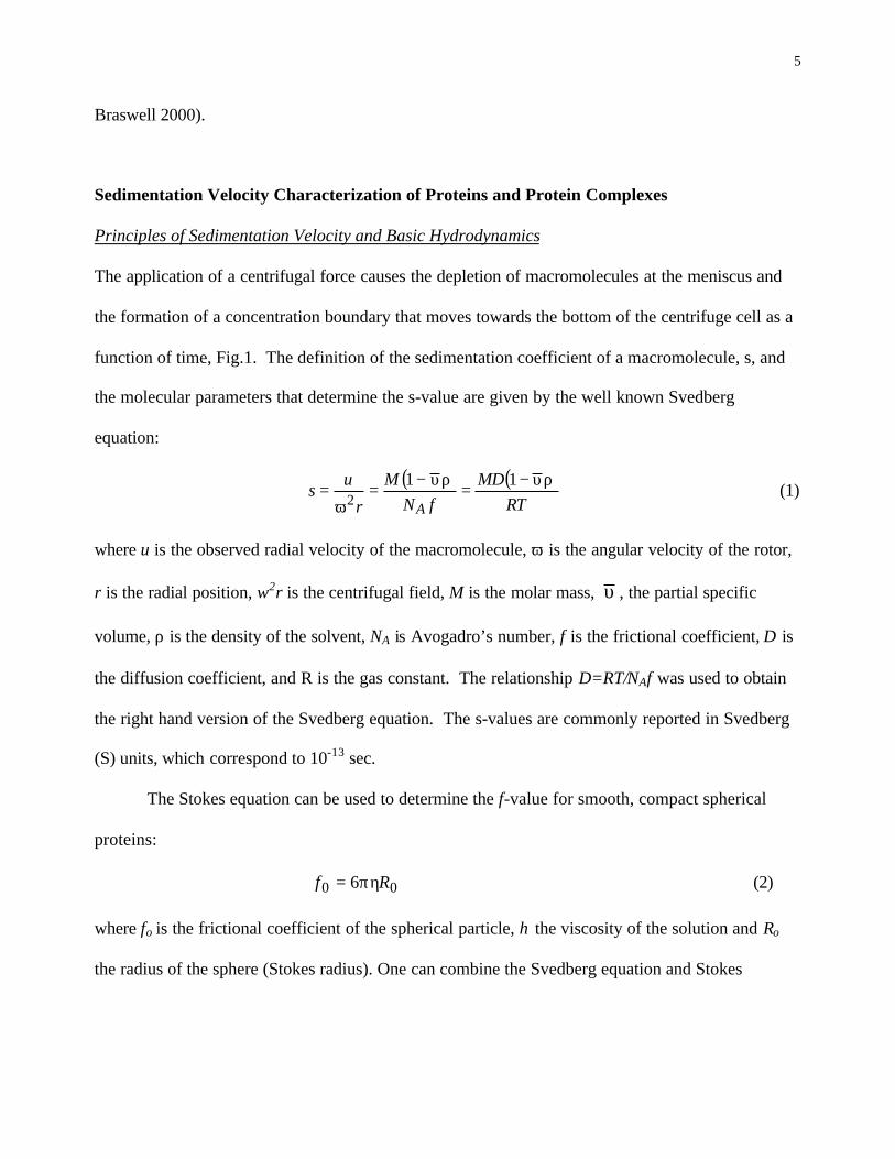
The application of a centrifugal force causes the depletion of macromolecules at the meniscus and

the formation of a concentration boundary that moves towards the bottom of the centrifuge cell as a

function of time, Fig.1. The definition of the sedimentation coefficient of a macromolecule, s, and

the molecular parameters that determine the s-value are given by the well known Svedberg

equation:

( ) ( )RT

MDfN

M

r

us

A

ρυ−=

ρυ−=

ω=

112 (1)

where u is the observed radial velocity of the macromolecule, ω is the angular velocity of the rotor,

r is the radial position, ω2r is the centrifugal field, M is the molar mass, υ , the partial specific

volume, ρ is the density of the solvent, NA is Avogadro’s number, f is the frictional coefficient, D is

the diffusion coefficient, and R is the gas constant. The relationship D=RT/NAf was used to obtain

the right hand version of the Svedberg equation. The s-values are commonly reported in Svedberg

(S) units, which correspond to 10-13 sec.

The Stokes equation can be used to determine the f-value for smooth, compact spherical

proteins:

00 6 Rf πη= (2)

where fo is the frictional coefficient of the spherical particle, η the viscosity of the solution and Ro

the radius of the sphere (Stokes radius). One can combine the Svedberg equation and Stokes

6

equation (Teller et al. 1979; van Holde et al. 1998), in which the Ro of the sphere is expressed as

3/1

43

π

υ

ANM

, to obtain

( )3/1

43

6

1

π

υπη

ρυ−=

AA

sphere

NM

N

Ms (3)

Substituting the values for all the constants (η for water at 20oC) yields Eq.4, the s value for a

sphere in terms of M, υ and ρ only (where M is in units of Da, s in S units, υ in ml/g and ρ in

g/ml ).

( )

-1 0.012 3/1

3/2

υ

ρυ=

Mssphere (4)

Using Eq. 4 one can predict the sedimentation velocity coefficients for smooth compact spherical

proteins in water at 20oC. This ssphere-value is the maximum s-value that can be obtained for a protein of

a given mass, since a compact sphere has the minimum surface area in contact with solvent and

consequently the protein would have a minimum frictional coefficient, fo. A correction of the

experimental s-value to a standard state of water at 20oC is necessary for comparative purposes of data

obtained from different laboratories as well as under different experimental conditions. The standard

correction equation is given below:

( )

( ) BT

BTBTw ss

,

20

20

,,,20 1

1ρυ−ρυ−

η

η= (5)

where T and B designate the values at the temperature and under the buffer conditions of the

experiment, and the index 20,w indicates standard conditions. The ratio of the maximum s-value to the

observed s-value, ssphere./s20,w , is equal to the ratio of the experimental frictional coefficient to the

minimum frictional coefficient, (f/fo), which measures the maximum shape asymmetry from a sphere.

7

The frictional ratio can also be determined from s-values under experimental conditions as the ratio of

the ssphere from eq.3 (substituting appropriate constants) divided by the experimental s value.

Characterization of Proteins Using Boundary Sedimentation Velocity

For the sake of simplicity, let us first consider a single component system. The motion of the boundary

as a function of time determines the s-value. Depending on the optical system chosen, this experiment

typically requires 0.05 to 0.5 mg of material. The software for the determination of s-values will be

described below. The evaluation of s20,w from the experimental s-value via Eq. 5 can be rapidly

accomplished using the public domain software program Sednterp (http://www.rasmb.bbri.org/)

developed by Hayes, Laue and Philo. Sednterp also provides rapid determination of the η and ρ for a

large variety of solutions. In addition, Sednterp calculates υ from the amino acid composition of the

protein. The latter can be imported from a data bank in either the one letter or 3 letter code for amino

acids. If one has access to an Anton-Paar DMA 5000 density meter or comparable precise density

measuring instrumentation, then υ values can be determined experimentally (Kratky et al. 1973)

(although this requires ~ 5mg, which may not be available). Once s20,w has been determined one can ask

the following question. Is the s20,w consistent with the sequence molar mass of a monomer? Eq. 4 can

be used to estimate the maximum s20,w -value for a monomer. If the experimental s20,w is significantly

higher, one can conclude that the quaternary state is not monomeric, while a lower value would indicate

an extended shape of the monomer due to a larger frictional coefficient. For example, let us assume

that you have a protein with a molar mass of 50 kDa and a υ of 0.730 ml/g and you perform a

boundary SV experiment in phosphate buffered saline and obtain an experimental s-value of 5.67 S.

This corrects to a s20,w of 5.87 S. Using Eq. 4, you would predict a maximal s-value of 4.93 S based on

the monomeric molar mass. Clearly the experimental s20,w is much higher than the predicted value for a

spherical monomer, pointing to self-association. A dimer would have a theoretical s20,w value of 7.77 S.

8

As indicated above, ssphere/s20,w measures the maximum shape asymmetry of the protein, f/f0, and for the

above example f/f0 would be 1.33 which supports the formation of a dimer with a moderately extended

shape.

We are now in position to do some basic hydrodynamic modeling of the putative dimer. The

total shape asymmetry f/f0 can be separated into two factors, a geometrical shape asymmetry and a

hydration expansion:

3/1

2

12

shape0

υ

υδ+υ=

ff

ff

(6)

The symbol δ denotes the hydration of the protein in grams of water per gram of protein, for which

a consensus value is commonly taken to be 0.3 g/g (Perkins 2001). The partial specific volume

subscripts 1 and 2 denote solvent and protein, respectively. The right-hand term in parenthesis is

the volume asymmetry due to hydration, or a hydration frictional ratio f/fhyd. In our example, since

f/f0 is 1.33, we obtain, with δ of 0.3 g/g, frictional ratios f/fhyd of 1.12 and f/fshape of 1.19. The

simplest hydrodynamic shape analysis consists in the approximation of the protein shape by a

prolate or oblate ellipsoid. Sednterp can determine f/fshape and the axial ratio of the respective

ellipsoid model. Our hypothetical protein dimer would be hydrodynamically equivalent to a prolate

ellipsoid with an axial ratio of 4, with axial dimensions of 17.3 nm (2a) and 4.3 nm (2b).

It is evident from the above example that we have gained considerable information from a

boundary SV experiment. It is also evident that the Sednterp software greatly facilitates the ability

to determine all the experimental parameters relevant in SV and performs basic hydrodynamic

calculations. Sednterp has a companion paper covering many of the points discussed above in

greater depth. (Laue et al. 1992). The help menu of Sednterp tersely covers hydrodynamic concepts

with references. For more advanced hydrodynamic concepts, the reader is referred to the reviews of

Teller et al. (Teller et al. 1979) and Garcia de la Torre (Garcia de la Torre 1992).

9

The above discussion of basic hydrodynamic principles opens for consideration the

questions of how the experimental s-value is extracted from the measured data, possible

deconvolution of multiple sedimenting components, and other advanced topics. These will be

discussed below.

Determination of Sedimentation Coefficients and Interpretation of Sedimentation Velocity

Experiments

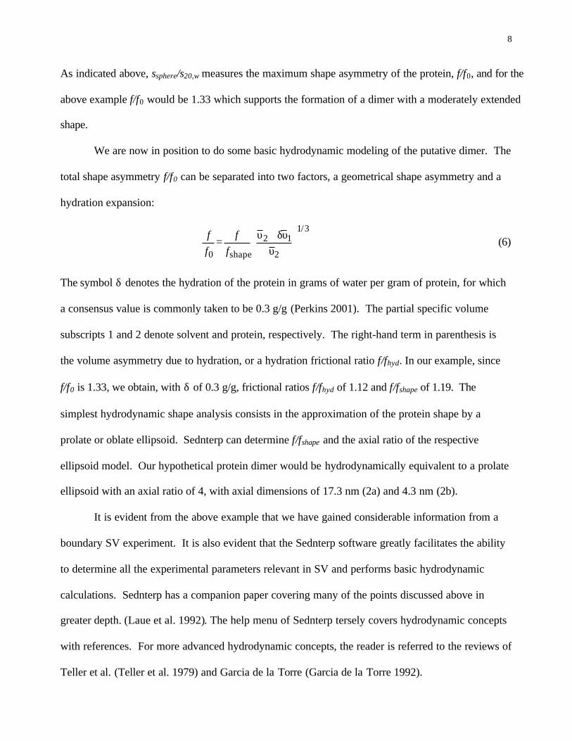
The data measured in AU are concentration profiles in the radial direction as a function of time

(Fig. 1). Hence, conceptually the simplest determination of a macromolecular sedimentation

coefficient is based on the formation of a sedimentation boundary in a high centrifugal field, where

the s-value might be determined, for example, by the displacement of the boundary midpoint (Fig.

1) (Svedberg and Pedersen 1940). However, this method is mainly of historical relevance, as

modern computational techniques have enabled much more powerful approaches, such as modeling

the data directly with the underlying transport equation (the Lamm equation):

χω−

∂χ∂

∂∂

=∂

χ∂),(

),(1),( 22 trrsr

trrD

rrttr

(7)

Eq. 7 describes the evolution of the concentration distribution of macromolecular species s as a

function of time and radial position under the influence of sedimentation and diffusion in the sector-

shaped ultracentrifugal sample cell (Lamm 1929).

Modeling the sedimentation data with the Lamm equation Eq. 7 takes full advantage of the

rich data basis of the full sedimentation process (Fig. 1), which can typically consist of 105 data

points with a signal-to-noise ratio between 100 and 1000. The precision of the sedimentation

coefficients increases with rotor speed, and typically is between 0.1 – 1%. Nonlinear least-squares

regression can be performed with several software packages operating on the Windows platform,

10

including LAMM (authored by J. Behkle and O. Ristau see ftp://ftp.rasmb.bbri.org/rasmb/spin/,

SVEDBERG (by J. Philo, http://www.jphilo.mailway.com/svedberg.htm) , and SEDFIT (by P. Schuck

http://www.analyticalultracentrifugation.com), or for the Unix environment ULTRASCAN (by B.

Demeler see http://www.ultrascan.uthscsa.edu/ ). LAMM and SVEDBERG use approximate analytical

solutions to Eq. 6 (Behlke and Ristau 1997; Philo 1997), while ULTRASCAN and SEDFIT use

different numerical finite element solutions (Demeler and Saber 1998; Schuck 1998). An advantage

of the latter approach is its generality, which allows sedimentation coefficients to be determined

even where no clearly visible boundary is formed, theoretically only requiring any molecular

redistribution as a result of the applied centrifugal force. In practice, SEDFIT can be used to model a

wide range of sedimentation processes, from the redistribution of salts (typically < 0.1 S) or the

sedimentation of small molecules, peptides, proteins and protein complexes, to large particles such

as virus capsids or dispersion particles (> 1000 S). Further, it allows determination of both

sedimentation and flotation coefficients (e.g. for detergents or lipoproteins with υ > 1/ρsol), and

modeling of experimental configurations generated with synthetic boundaries where the initial

distribution is not uniform (such as analytical zone centrifugation (Lebowitz et al. 1998), see

below). SEDFIT also has a comprehensive set of tools adjusting the analysis for the special noise

structure of interference optical data (Schuck and Demeler 1999). A detailed online help system

and several introductory tutorials are available. Recently, a version of SEDFIT for global modeling

of multiple experiments (including sedimentation equilibrium and dynamic light scattering) has

been introduced, SEDPHAT, and applied for the simultaneous fit of sedimentation velocity

experiments at different rotor speeds, with improved resolution of different species.

As usual when modeling experimental data, the analysis results in measures of goodness-of-

fit (e.g. the rms error of the fit and the distribution of the residuals), which allow assessment if the

model satisfactorily describes the sedimentation process. If a solution to the Lamm equation Eq. 7

11

(or a superposition of a small number of Lamm equation solutions) is not a good model, it is

possible that either a larger number of different sedimenting species are present, and/or that

chemical reactions are present (reversible interactions) on the time-scale of the sedimentation

experiment. Both cases can be distinguished from the details of the time-course of sedimentation,

and from the concentration dependent sedimentation behavior exhibited by interacting proteins.

Analysis of Size-Distributions

The analysis of multi-component protein mixtures or protein samples with possible

contamination by peptides or aggregates can be of considerable importance for a complete

characterization of a protein system under investigation. Such systems may have resolvable

sedimentation species and one would observe two or more boundaries as a function of time.

However, diffusional spreading of components often leads to only a single observable boundary

composed of non-resolved multiple sedimenting components. Fig. 1 shows a single boundary for a

BSA sample that was composed of a partial proteolytic break down product, non-resolved

monomers and oligomeric species based on size exclusion chromatography. We will use this

sedimentation boundary data to illustrate the analysis of size distributions by different

computational treatments.

For the past decade two approaches have been used extensively for unraveling sedimenting

components: the integral sedimentation coefficient distribution G(s) (van Holde and Weischet

1978); and the dc/dt method for calculating a differential apparent sedimentation coefficient

distribution g(s*) (Stafford 1992). The G(s) method is based on a geometric division of the

sedimentation boundary and attempts to resolve sedimenting species by extrapolating each

boundary division to infinite time in order to eliminate the effect of diffusion on sedimentation. The

extrapolated s-values for each boundary fraction produce an integral sedimentation coefficient

12

distribution G(s) (for review see (Hansen et al. 1994)). An adaptation of this methodology to the

noise structure of interference optical data has been described (Schuck et al. 2002). It is

implemented in the software ULTRASCAN and SEDFIT. The G(s) method has great diagnostic value

for the presence of heterogeneity and of attractive or repulsive interactions (Hansen et al. 1994;

Demeler et al. 1997). Characterization of the lipid free form of the apolipoprotein A-1 used the van

Holde-Weischet G(s) method to show the conformational plasticity of the protein and how amino

terminal deletions reduced conformational transitions significantly (Rodgers et al. 1998a; Rodgers

et al. 1998b).

Stafford’s dc/dt approach subtracts closely spaced boundary scans to approximate a set of

time derivative dc/dt vs. radius profiles. Based on the equation for sedimentation of an ideal non-

diffusing species, the radial coordinate is transformed into an s-value, designated s*, and the time

derivative dc/dt is transformed into dc/ds, which is a differential sedimentation coefficient

distribution, designated g(s*). g(s*) distributions can be computed with the software DCDT+

developed by J. Philo (http://www.jphilo.mailway.com/dcdt+.htm). This method has been very

successful, in part because of the invariance of dc/dt with respect to the systematic noise structure of

interference optical ultracentrifuge data. However, no correction for diffusion is made, which limits

the resolution (see below). Further, the approximation of dc/dt with finite differences of sequential

scans causes constraints in the rotor speed and the number of scans that can be analyzed (Philo

2000a). More recently, a least-squares variant of the apparent sedimentation coefficient distribution

from direct boundary modeling (with Eq. 7 and taking D = 0) has been introduced, termed ls-g*(s)

and implemented in SEDFIT, which eliminates some of these constraints and can be applied equally

to absorbance and interference data (Schuck and Rossmanith 2000). The g*(s) method has been

reviewed by Laue (Laue 2001). An example from our work is the use of the g*(s) analysis to

monitor the binding of the SmtB repressor to different DNA target sequences and the hydrodynamic

13

characterization of the binding data. These results were coupled with SE for determining the

protein-DNA stoichiometry, which provided a working model for the formation of the repression

complex (Kar et al. 2001).

More recently, a differential sedimentation coefficient distribution that deconvolutes

diffusion effects, based on direct boundary modeling with a distribution of Lamm equation

solutions, has been implemented. In brief, a sedimentation coefficient distribution c(s) can be

defined as

ε+χ= ∫ dstrsDssctra ),),(,()(),( (8)

with a(r,t) denoting the observed sedimentation data, c(s) the concentration of species with

sedimentation coefficient between s and s+ds, and χ(s,D(s),r,t) the Lamm equation solution

described above. Recently, mathematical methods for solving Eq. 8 have been described, using

maximum entropy regularization and implemented in SEDFIT (Schuck 2000). Different variants for

estimating the relationship of s and D for mixtures of globular proteins are available, with the most

general one based on a weight-average shape factor f/f0 that can also be extracted from the

experimental data. Conversion of the c(s) distribution into a molar mass distribution c(M) is

possible. Because of the assumption of a weight-average shape factor f/f0, it may not lead to

correct molar mass values for all species. In contrast, the approximation of diffusion by a weight-

average shape factor f/f0 has virtually no effect on the peak value of the sedimentation coefficient

distribution. For cases where the molar mass of the main species is known, this can be used as a

prior knowledge in the calculation of c(s). More details are described in Schuck (Schuck 2000;

Schuck et al. 2002).

The result of a c(s) sedimentation coefficient distribution for the data from Fig. 1 is shown in

Fig. 2. It is apparent that the sedimentation coefficient distribution that has been deconvoluted is

14

conceptually similar to a chromatogram from gel-filtration. However, it should be noted that the

separation is achieved without resorting to interactions with a matrix, that it is based on differences

in mass and friction, with the former more strongly size-dependent (~M2/3) than the Stokes radius

(~M1/3), and that sedimentation coefficient distributions have a much wider dynamic range.

Although the diffusional broadening in the raw data is less in gel-filtration, the database in

sedimentation is very large and its solid foundation on first-principles allows for diffusional

deconvolution. The s-value of each peak can be interpreted as described above. It is apparent from

the c(s) curve in Fig. 2 that the BSA monomer, dimer, and trimer are baseline separated (and

resolved from a small degradation product at 2.7 S). Fig. 2 also compares results from using the

G(s) and g*(s) approaches. Although both indicate the presence of different BSA oligomers,

neither technique is successful in resolving them. It has been argued that the results from g(s*) are

conceptually similar to those of c(s) (Laue 2001) but a very clear qualitative difference in the

resolution is apparent when comparing a g(s*) analysis on our BSA data (dotted line) with the c(s)

curve (solid). A detailed analysis and comparison of the different size-distribution methods in

theory and practice can be found in (Schuck et al. 2002).

In our laboratory, the determination of the number of species present by c(s) usually

precedes the modeling with a discrete number of Lamm equation solutions described above. Many

examples for the use of c(s) in the study of protein oligomeric state, self-association and

conformational changes have been published (Perugini et al. 2000; Schuck et al. 2000; Cole and

Garsky 2001; Hatters et al. 2001a; Lacroix et al. 2001; Arthos et al. 2002; Chang et al. 2002).

Analysis of Interacting Systems Using Sedimentation Velocity

For the study of the thermodynamic aspects of self-association or hetero-association, SE is

usually the method of choice (see below). However, SV can be applied when the proteins do not

15

exhibit sufficient stability for the extended time required in SE, and in many cases it gives a wealth

of complementary information beyond the thermodynamics of molecular interactions. The study of

self-associating systems by SV can give information about the association scheme, sedimentation

coefficients and hydrodynamic shape of the reversibly formed oligomers in solution, which can be

used to build simple geometric models for assembly of the oligomers (among recent examples are

(Rivas 2000; Schuck et al. 2000; Correia 2001; Kar et al. 2001). Further, the comparison of the

equilibrium constant obtained in SV and SE shows the pressure dependence of the association, and

can indicate volume changes associated with the interaction.

A traditional strategy for the sedimentation analysis of self-associating and hetero-

associating systems is the determination of the weight-average sedimentation coefficient sw(c) as a

function of concentration (sw can be derived, for example, via integration of any of the differential

sedimentation coefficient distributions c(s), g(s*) or ls-g*(s), see above). If the experiments are

conducted at sufficiently high rotor speeds to generate a solution plateau, sw is only a function of the

chemical composition at the plateau concentration, and the concentration dependence of sw(c) can

be analyzed by fitting the binding isotherm with mass action law models (Rivas et al. 1999; Correia

2000) .

For slow self-associations, all the size-distribution methods described above can still be

used, with c(s) usually resolving sedimentation coefficients of monomers, dimers, and higher

oligomers (Perugini et al. 2000), while separating possible degradation products and aggregates.

However, if there are any molecular interactions on the time-scale of sedimentation, the

sedimentation behavior will be dependent on concentration and rotor speed, and the

sedimentation/reaction/diffusion process becomes significantly more complex. In this case, the

application of the size-distribution methods involving diffusional deconvolution (c(s) and G(s)) can

only give qualitative and diagnostic information. In particular, the modeling of the sedimentation

16

boundary as a superposition of Lamm equation solutions for non-interacting species, c(s), can lead

to misleading or artifactual details on the size-distribution. However, the weight-average

sedimentation coefficient, as obtained by integration of the differential sedimentation coefficient

distributions is a correct representation of the system.

Another approach for rapid interactions, which has only recently become generally

available, is based on the direct modeling of the sedimentation profiles (similar to Fig. 1) with Eq.

7, modified to allow concentration-dependent sedimentation and diffusion coefficients (Cox 1969).

For self-associating proteins with unknown oligomeric states, this allows taking advantage of the

distinct sedimentation patterns generated by different self-association schemes. SEDFIT has several

models for proteins in rapid reversible self-association equilibrium (Schuck 1998). A strategy for

the treatment of hetero-associations has been reported (Stafford 2000). One difficulty can be that

the number of free parameters required for the complete characterization of protein self-association

can exceed the information content of a single SV experiment. Therefore, prior knowledge can be

inserted in the form of the monomer molar mass from amino acid sequence, monomer or oligomer

sedimentation coefficient from SV under very dilute or highly concentrated conditions, or

association constants known from SE (if there is no pressure-dependence of the association).

However, global modeling techniques (for example in SEDPHAT) allow one to reduce the need for

additional prior knowledge. Another form of interaction that can be globally modeled in this way is

caused by thermodynamic and hydrodynamic non-ideal solutions, which has been used to measure

the second virial coefficient in the study of crystallization conditions (Solovyova et al. 2001). Since

the direct modeling approach has more stringent requirements for sample purity than an analysis of

sw(c), but can require fewer experiments, the choice of method may be dictated by practical

considerations.

17

Boundary Shape Analysis for the Determination of Molar Mass

As pointed out above, the Svedberg equation Eq. 1 relates the sedimentation and diffusion

coefficients with the buoyant molar mass, and it is therefore possible to determine the molar mass

from the boundary shape of SV profiles. (Or conversely, knowledge of the buoyant molar mass of

the protein from amino acid composition or from SE can be used as prior knowledge to improve the

resolution of the data analysis.) In contrast to the sedimentation coefficients, the precision of the

molar mass determination increases with lower rotor speed, converging to the approach to SE (see

below). While the molar mass from the boundary shape is more susceptible to artifacts arising from

the sedimentation process, it has the important practical advantage of its relative rapidity.

When determining the molar mass from the boundary shape, one difficulty is that

heterogeneous populations of macromolecules with slightly different s-values can cause boundary

spreading. For the latter case the uncritical application of Eq. 1 using an average s-value and the

apparent diffusion coefficient will lead to an apparent molar mass significantly smaller than true

(average) molar mass. This problem can be diagnosed by a sedimentation coefficient exceeding the

maximum s-value for the apparent molar mass using Eq. 3. Conversely, repulsive macromolecular

interactions decrease s but can also reduce boundary spreading, leading to an erroneous apparent

molar mass. When working with globular proteins, these repulsive interactions can usually be

avoided at concentrations below 1 mg/ml and sufficient supporting electrolyte (for most proteins

50-100 mM). If the s-value decreases with increasing concentration, in the absence of charge

effects, then hydrodynamic interactions are affecting the sedimentation process, which are governed

by the frictional asymmetry of the particle (Rowe 1992). Both of these factors lead to

sedimentation profiles distinctly different from those shown in Fig. 1, and can be detected by

critical inspection of the residuals of a direct boundary model. A detailed description of

sedimentation under non-ideal conditions can be found in (Solovyova et al. 2001) where

18

sedimentation boundary profiles were modeled with modified transport equations for the purpose of

exploring protein crystallization conditions.

In practice, the most reliable determination of the molar mass is obtained by direct boundary

modeling with a small number of discrete (preferably a single) Lamm equation solutions (Eq. 7).

This analysis can be accomplished, for example using LAMM, SVEDBERG, and SEDFIT, or the

modeling of the time-derivative dc/dt with the approximate Lamm equation solutions with DCDT+

(as recently introduced by Philo (Philo 2000a)). An older technique of modeling of the apparent

sedimentation coefficient distributions g*(s) with Gaussians also gives a molar mass estimate, but

this is considerably less precise and requires more constrained experimental conditions (Schuck and

Rossmanith 2000). As indicated above, size-distribution methods for molar mass distributions have

been recently described and are implemented in SEDFIT (Schuck 2000), but these are inherently

more difficult to determine than the sedimentation coefficient distributions. An example for its

application to small nucleic acid complexes has been reported by Hatters et al. (Hatters et al.

2001b). Microheterogeneity due to compositional variation such as glycosylation (see below) or

differing conformations will present difficulties determining molar mass by sedimentation velocity

methodologies.

Analytical Zone Centrifugation or Band Centrifugation

An alternative SV methodology was developed by Vinograd et al. (Vinograd et al. 1963) thirty-

nine years ago (originally designated band centrifugation), and recently reexamined (Lebowitz et al.

1998). Instead of starting the experiment with a uniform loading of the sample solution, in this

method, upon initiation of the centrifugal field, the macromolecules are transferred from a small

well containing 20-30 µl on top of a column of solvent of greater density (e.g. by a difference in

NaCl concentration or the presence of D2O) than the macromolecular solution. A self-generating

19

density gradient occurs by diffusion of small molecules from the main liquid column into the

transferred macromolecular lamella. Although this diffusional density gradient is very small (and

distinctly different from the more commonly used density gradients that are preformed or formed by

sedimentation) it is sufficient to prevent convection and stabilizes the sedimenting zone or band of

macromolecules. Very recent results from this laboratory have shown that AZC data can be

modeled with the transport equations (Eqs. 6 and 7) implemented in SEDFIT (manuscript in

preparation). More details and applications can be found in (Lebowitz 1994; Lebowitz et al. 1994;

Lebowitz et al. 1998; Kar et al. 2001).

Analytical zone centrifugation (AZC) can represent an attractive approach to conventional

boundary SV of proteins and protein complexes with the major advantages of employing

approximately 1/20th as much material as conventional boundary analysis, and the potential for

physical separation of sedimenting species. Hence, sedimentation coefficients are easily obtained

with only µg quantities of protein. Since the protein zones rapidly sediment into the bulk column

solution, AZC also allows for either ion or pH exchanges. Consequently, investigators can study

the effects of environmental changes on proteins or protein complexes with small amounts of

material. For the case of DNA, the AZC characterization of pH induced conformational transitions

of polyoma DNA played a key role towards the discovery of supercoiled DNA (Vinograd et al.

1965). Also, the economy in sample volumes of AZC can be advantageous when studying the

effects of temperature. For example, the thermal stability of the human immuno-deficiency virus-1

reverse transcriptase heterodimer was monitored using AZC (Lebowitz et al. 1994).

Sedimentation Equilibrium Measurements

At centrifugal fields lower than those generally used for SV, sedimentation is balanced by

20

diffusional transport, and SE is achieved when the net transport vanishes throughout the solution. It

can be easily established by running the centrifuge until the concentration distribution appears to be

invariant with time. In equilibrium, the concentration distribution generally approaches an

exponential (for derivations see van Holde et al. (van Holde et al. 1998)), and for a mixture of non-

interacting ideally sedimenting solutes, the measured signal as a function of radial position, a(r),

takes the following form:

( ) )(

21

exp)( 20

22

0, δ+

−

ωρυ−ε= ∑

n

nnnn rr

RTM

dcra (9)

where the summation is over all species n; cn,0 denotes the molar concentration of species n at a

reference position r0. Mn , nυ and εn denote the molar mass, partial specific volume, and the molar

extinction coefficient, respectively. d is the optical path length (usually 1.2 cm), and δ is a base line

offset, which compensates for differences in non-sedimenting absorbing solutes between sample

and reference compartments and small non-idealities in the cell assemblies and data acquisition.

Similar to SV, repulsive interactions between proteins will lead to non-ideal sedimentation

equilibrium, which can usually be avoided at concentrations below 1 mg/ml and with supporting

electrolyte of 100 mM. When using the interference optics, the extinction coefficient in Eq. 9

should be replaced by a specific signal increment, and the baseline offset is usually radial

dependent, requiring separate experimental determination (Ansevin et al. 1970). For a detailed

description of practical aspects of planning, conducting, and analyzing a SE experiment, such as

choice of optical system, buffer conditions, rotor speeds, experimental time, sample purity, sample

volume, etc., see (Schuck and Braswell 2000).

Eq. 9 states that the exponential distribution at SE is the sum of the exponentials of the

macromolecular species present in solution. The concentration of each component varies

21

exponentially with r2/2 as a function of ( ) RTM nn 21 2ωρυ− . The term ( )ρυ−1M is the buoyant

or reduced molar mass, i.e., following Archimedes principle, the mass of a macromolecule acted on

in solution by the centrifugal field is reduced by the mass of the displaced solvent. For a single

protein only one exponential distribution will be present which readily allows for the determination

of the buoyant molar mass of this molecule, and with knowledge of the υ of the protein the molar

mass is readily evaluated. Classically, Eq. 9 was converted to a linear form and the weight-average

molar mass determined from the slope. Currently, computational software can readily fit an

exponential model to determine the molar mass. In fact, the power of global non-linear regression

fitting of multiple data sets has enormously extended the applications of SE to complex systems. A

number of these applications will be discussed below.

Self-Associating Systems

As indicated above, interacting systems are of particular interest to protein scientists. With some

modifications to introduce equilibrium constants and mass action law, Eq. 9 also describes the SE of

reversibly formed protein complexes. For self-associating systems, we can relate the molar

concentration at the reference point of all oligomeric species via cn,0=Kn(c1,0)n (with the subscript 1

denoting the monomer). In addition, for Mn we substitute nM1 in each exponential term. If no

change in the volume of the protomers accompanies the self-association ( υ is constant) we obtain

( )

1 )(21

exp)()( 12

02

21

1,01 =δ+

−

ωρυ−ε= ∑ Kwithrr

RTnM

cdKnran

nn (10)

It should be noted that association constants are defined from the monomer to the n-mer.

Intermediate association constants are readily calculated once the Kn values have been determined.

Using Eq. 10 we are in position to perform global non-linear regression fitting of multiple SE data

22

sets at different loading concentrations and rotor speeds to determine the monomer molar mass, Kn -

values, and stoichiometries for selected association models that best fit the data. An excellent

Beckman-Coulter Instruments monograph on the analysis of self-associating systems has been

prepared by McRorie and Voelker (McRorie and Voelker 1993). It offers the reader very practical

steps for self-association modeling, including error analysis. As pointed out above, SV

measurements provide a good basis for selecting the association model.

Sedimentation Equilibrium With Glycoproteins

Many eukaryotic and viral proteins are heavily glycosylated with a heterogeneous

distribution of carbohydrates. This situation often leads to anomalous behavior on size exclusion

chromatography and SDS PAGE. In contrast, AU offers a more rigorous methodology for the

determination of the molar mass and the oligomeric state in solution. A complication is the partial

specific volume of a glycoprotein, which leads to a buoyancy that is different from non-

glycosylated proteins, and is strictly dependent on the carbohydrate composition. Ideally, one could

measure the υ of the glycoprotein using a density meter, however material limitations often

preclude this approach. For determination of the extent of glycosylation, ultracentrifugal methods

have been described (Shire 1992; Lewis and Junghans 2000). Alternatively, it is frequently possible

to determine the extent of glycosylation for a monomer by mass spectrometry (MS), if combined

with the molar mass of the protein from the amino acid composition (Fairman et al. 1999). This

allows the use of ultracentrifugal data to determine the oligomeric state in solution. In this case, the

partial-specific volume can be expressed in terms of weight fractions for the protein and

carbohydrate moiety, wp and wc, and the protein and carbohydrate partial-specific volumes υ p and

υ c, respectively (Shire 1992). If carbohydrate composition data are available the υ c can be

determined for different N-linked oligosaccharides (Shire 1992; Fairman et al. 1999; Lewis and

23

Junghans 2000). However, if the carbohydrate composition is unknown, one can use estimates for

average υ c of carbohydrates, which translates to uncertainties in the value of molar mass of the

glycoprotein of usually only a few percent (Lewis and Junghans 2000).

This approach was used by Center et al. (Center et al. 2000) for the analysis of the HIV-1

recombinant gp120. Obviously, for a monomeric glycoprotein there should be good agreement

between the weight-average molar mass determined by MS and SE, and this was the case for gp120

cited above. For self-associating proteins, the SE results can reveal the oligomeric state and

association constants. (Fairman et al. 1999) applied the above principles to the characterization of T

cell and B cell receptors using SE and electrospray MS analysis to obtain cυ .

Characterization of Membrane Proteins Using Sedimentation Equilibrium

Due to their hydrophobic nature integral membrane proteins require non-ionic detergents for

solubilization in a functional state. The solubilization process involves the formation of protein-

detergent micelle complexes. Consequently, a molar mass determination by SE would yield the

sum of the protein mass and the mass of bound detergent. Although this is, in principle, not a

problem for the study of hetero-associations of membrane proteins, it provides a significant

complication for measuring the molar mass and the self-association properties. Reynolds and

Tanford (Reynolds and Tanford 1976) developed an ingenious methodology for the determination

of the protein molar mass in protein-detergent complexes without direct knowledge of detergent

binding. The buoyant molar mass of a protein-detergent complex can be decomposed into a term

for the protein and term for the detergent respectively:

( ) ( ) ( )ρυ−+ρυ−=ρυ− DDpPcc MMM 111 (11)

The subscripts p, D, and c denote protein, detergent, and protein-detergent complex, respectively. If

24

the density of the solution is adjusted with an appropriate solute to match the density of the

detergent ( Dυ=ρ /1 ) then the detergent becomes ‘graviationally transparent’ and the term

( )ρυ− DDM 1 will vanish. Hence, the SE concentration distribution only reflects the molar mass of

the protein.

A review of the interaction of membrane proteins and lipids with solubilizing detergents has

recently been published (le Maire et al. 2000). It lists the properties of detergents commonly used

for the solubilization of membrane proteins, such as the critical micelle concentration and Dυ .

Past SE work has relied almost exclusively on using H2O:D2O mixtures for density matching with

considerable success (Reynolds and Tanford 1976; Tanford and Reynolds 1976; Reynolds and

McCaslin 1985; Schubert and Schuck 1991). Recently sucrose, glycerol and Nycodenz solutions

have been employed successively for density matching (Mayer et al. 1999; Lustig et al. 2000).

Preferential hydration of the micelles (and also the protein) can occur in these solutions, which can

significantly decrease the matching density in sucrose, glycerol and Nycodenz solutions compared

to H2O:D2O mixtures. Therefore, these solute additives can provide greater experimental versatility

for detergent selection and the solution preparation. In addition, sucrose and glycerol are known to

stabilize proteins which is advantageous for membrane proteins that may be labile. For a

description of methods for determining the density of the detergent, see (Mayer et al. 1999; Lustig

et al. 2000). In these studies, the density additives discussed above did not introduce non-ideal

sedimentation behavior nor significant changes in the partial specific volume of the membrane

protein (Mayer et al. 1999; Lustig et al. 2000). The effects of different sugars on ( )ρυ-1 of muscle

adolase have been recently explored in order to probe protein-sugar interactions (Ebel et al. 2000).

This study allows an estimate of the error in the molar mass due to the change in υ of the protein

by the addition of sucrose. At a sucrose density of 1.04 (9.7%) the error in molar mass would be

25

approximately 4%. Although this error estimate may vary with different proteins and in the

presence of detergents, it supports the evaluation of the stoichiometry of a membrane protein or

complex using sugar additives. If density matching of a detergent requires large concentrations of

an additive significant errors may result due to large changes in the partial specific volume, non-

ideal behavior and density gradient formation of the additive ((Mayer et al. 1999)). An alternative

to direct density matching for high additive concentrations is to perform a series of sedimentation

equilibrium experiments at different solvent densities and to extrapolate the results to the matching

density of the detergent ((Tanford and Reynolds 1976; Schubert and Schuck 1991; Lustig et al.

2000) ) .

Very recently we have measured the molar mass of SIV-1 envelope complex purified

directly from the virus. After cross-linking of the surface exposed membrane proteins gp120 and

gp41, hydrogenated triton X-100 was used for solubilization of the complex from virion membranes

and the molar mass measured using density matching with sucrose. The stoichiometry of the env

complex was found to be trimeric and this could be visualized in the electron microscope (Center et

al. 2001). The mass measurements from SE were in very good agreement with mass measurements

from scanning transmission electron microscopy (Center et al. 2001). The density matching

methodology allows for the characterization of membrane protein self association (Schubert and

Schuck 1991; Fleming et al. 1997; Fleming and Engelman 2001). It should be pointed out that

association may be dependent upon the type of solubilizing detergent (Musatov et al. 2000). For

cases where membrane proteins are unstable it is possible to do global analysis of SV data under

density matching conditions to determine molar mass (Robinson et al. 1998). Density matching has

also been extended to the analysis of the oligomeric state of the erythrocyte band 3 protein

reconstituted in small unilamellar lipid vesicles (Lindenthal and Schubert 1991). For a review of

the quaternary structure and function of transport proteins with numerous citations to analytical

26

ultracentrifugation characterization see (Veenhoff et al. 2002).

Heterogeneous Interactions

For purposes of this discussion, heterogeneous interactions are defined as interactions where two (or

more) reactants reversibly form a complex with a specific stoichiometry. Such interactions would

follow association schemes as, for example, A + B ⇔ AB; A + 2B ⇔ AB2; AB + B ⇔ AB2; etc.

Equilibrium constants over the range of 104 to 108 are readily measured and under certain

circumstances, both lower and higher equilibrium constants can be obtained. Additionally, the

stoichiometry of the interaction can usually be determined. For the present purpose, let us consider

the SE characterization of the simple reaction A + B ⇔ AB. This requires the study of the

components A and B alone, as well as mixtures of A and B at different molar ratios (including

equimolar). As above, it is convenient to introduce the buoyant molar mass as M*=M(1- υ ρ), and

SE experiments of solutions containing the separate components will allow us to determine the

values of M*A and M*B. These values may include contributions from glycosylation or detergent

micelles, which do not need to be known or further specified for the study of hetero-associations.

For the AB complex, we make the reasonable assumption that the partial specific volume of the AB

complex can be calculated from the respective weight fractions of the partial specific volume of

components A and B, hence M*AB = M*A + M*B. For the A + B ⇔AB reaction we have three

species in solution, free A and B and the AB complex, which in chemical equilibrium obey the mass

action law cAB= cAcBKAB. At equilibrium in the centrifugal field, the radial distribution is

(analogous to Eq. 10):

27

( ) )(

2exp)(

)(2

exp )(2

exp)(

222**

,.,.

222*

,.22

2*

,.

δ+

−

ω+ε+ε

−

ωε+

−

ωε=

oBA

BAABoBoA

oB

BoBoA

AoA

rrRTMM

dKcc

rrRT

Mdcrr

RTM

dcra

(12)

The major difficulty for fitting the parameters of this heterogeneous interaction model is the ability

to evaluate the contribution of the complex formed and the uncomplexed reactants to the total

signal. This usually requires global modeling of data acquired at different loading concentrations

and rotor speeds. However, one of the great advantages of the absorption optical system is that the

ability to scan at a variety of wavelengths, which greatly simplifies the analysis for spectrally

distinct proteins, and makes it possible to study heterogeneous interactions that would otherwise be

impossible.

The characterization of protein-DNA interactions represents an important area where multi-

wavelength absorbance analysis of SE data has been successfully applied. A target oligonucleotide

and DNA binding protein have significantly different absorption spectra and one can select a range

of wavelengths such that the resulting scans vary from the signal being dominated by the

oligonucleotide to the signal being dominated by the protein. This can be combined with global

analysis using independently determined extinction coefficients (Kim et al. 1994; Bailey et al. 1996;

Cole et al. 1997)(Cole et al. 1997); (Lee 2001) . It should be pointed out that the above multiple

wavelength analysis assumes that there is no change in the extinction coefficients of the reactants

upon binding, i.e., no hypo or hyperchromic shift at the scanned wavelengths and εAB = εA + εB.

This can be experimentally examined by measuring the sum of the absorbance of each component

using a dual compartment cuvette in comparison to the absorbance of the mixture of reactants under

conditions where substantial complex formation occurs (Bailey et al. 1996). For the situation where

there is a substantial extinction coefficient change upon complex formation a methodology has been

28

developed that combines absorption spectra scanned at multiple radii and radial profiles scanned at

multiple wavelengths (Schuck 1994) . This provides a two-dimensional data surface that can be

analyzed to achieve a simultaneous detection of the components extinction spectra and the other

variables in the SE model.

Another example of multiple wavelength SE is the study of the association of small peptides

with much larger proteins. The problem here is that the mass of the peptide-protein complex differs

so little from that of the protein alone that it is difficult to discriminate between them from the radial

distribution alone. However, if the peptide can be synthesized with 5-hydroxy tryptophan

incorporated into the molecule (Laue et al. 1993), it is spectrally distinguishable from the protein.

The extinction coefficients at the different wavelengths can be calculated from the ratios of the

observed scans of the reactants and the equilibrium constant can be obtained by globally fitting

appropriate models to the scans (Yoo and Lewis 2000).

SE analysis of both self-associating and hetero-associating proteins can be greatly facilitated

if the total amount of soluble protein remains constant during the time-course of the experiment

(see, for example, (Becerra 1991)). This approach has been recently reviewed by Philo (Philo

2000b). Binding constants of small absorbing molecules to proteins have very recently been

determined using the multi-wavelength strategy coupled with conservation of mass methodology

(Arkin and Lear 2001).

Software for Sedimentation Equilibrium Analyses

Non-linear least-squares parameter estimation is the major numerical method for SE data analysis.

An examination of the biophysical/biochemical literature will reveal the use of diverse software.

Since computational skills vary considerably, we believe that investigators should evaluate the

software outlined below based on their particular research applications and individual

29

computational data analysis expertise. With respect to commercial mathematical modeling

programs we cannot endorse one program over another.

For molar mass analysis and self-associating systems, the program NONLIN, developed by

Yphantis and Johnson at the National Analytical Ultracentrifuge Facility (NAUF) of the University

of Connecticut Biotechnology Center, has been applied extensively. Beckman-Coulter Instruments

supplies with each XLA and XLI purchased a data acquisition and analysis software package, which

includes a version of the NONLIN, program based upon the OriginTM software by MicroCal Inc. It

also includes a subtraction of data utility to allow for the determination of when SE has been

reached. (A more advanced software for testing attainment of equilibrium is WINMATCH,

developed at NAUF.) There are additional useful utilities including a data simulator. Investigators

can obtain from NAUF the most current program WINNONLIN and other programs for editing and

examining the SE data from single component and self-associating systems. There is an

organization entitled Reversible Associations in Structural and Molecular Biology (RASMB)

http://www.bbri.org/RASMB/rasmb.html that has an archive of AU software. Very recently the SE

data analysis software ULTRASPIN has been developed by the Center for Protein Engineering,

Medical Research Council, University of Cambridge (available from the Web site http://www.mrc-

cpe.cam.ac.uk/ultraspin/ free to academic/non-profit laboratories and for a small charge to

commercial investigators). ULTRASPIN can fit twenty different models. Multi-wavelength fitting is

provided for several protein-DNA interaction models and for several heterogeneous protein

interactions. For the Unix or Linux environment, SE analysis can be performed with the software

ULTRASCAN from Borries Demeler at http://www.ultrascan.uthscsa.edu./.

Curve fitting tools of commercial software such as SigmaPlot, IgorPro or KaleidaGraph

have been used. The MLAB software (Civilized Software) is a command line advanced

mathematical and statistical modeling system that has been used by this laboratory for many years.

30

There are many other commercial programs for non-linear regression modeling that can be found on

the Web.

Conclusions

As mentioned above, the scope of this short review did not allow descriptions of many topics and

applications of AU. Other reviews cited above should be consulted as well as SV and SE

methodological treatments that have been published in Methods in Enzymology. For example see

(Laue and Stafford 1999) and (Rivas et al. 1999). We have provided a tutorial review building from

the basic concepts to advanced AU approaches for the characterization of protein systems. We have

focused on what can be learned about proteins and their interactions using AU, and have given

sufficient information to allow protein scientists to take the practical steps towards reaching these

goals. Investigators should be encouraged to use both SV and SE to characterize their systems to

gain the maximum information possible. It should be noted that Beckman-Coulter Instruments

offers customers a 3-day course on the operation of the XLA/XLI. This course is intended for

beginner operators with minimal background in AU. For more advanced training, the NAUF of the

University of Connecticut Biotechnology Center offers a workshop in SV and SE data analysis.

Finally, there is a discussion group in the RASMB network of investigators who are interested in

the reversible interactions of macromolecules, to which one can readily subscribe

http://www.rasmb.bbri.org/.

31

REFERENCES

Ansevin, A.T., Roark, D.E., and Yphantis, D.A. 1970. Improved ultracentrifuge cells for high-speedsedimentation equilibrium studies with interference optics. Anal. Biochem. 34: 237-261.

Arkin, M., and Lear, J.D. 2001. A New Data Analysis Method to Determine Binding Constants ofSmall Molecules Using Equilibrium Analytical Ultracentrifugation with AbsorptionOptics.Anal. Biochem. 299: 98-107.

Arthos, J., Cicala, C., Steenbeke, T.D., VanRyk, D., Dela Cruz, C., Khazanie, P., Selig,S.M.,Hanback, D.B., Nam, D., Schuck, P., et al. 2002. Efficient inhibition of HIV-1 viralreplication by a novel modification of sCD4. J.Biol.Chem. 277: 11456-11464.

Bailey, M.F., Davidson, B.E., Minton, A.P., Sawyer, W.H., and Howlett, G.J. 1996. The effect ofself-association on the interaction of the Escherichia coli reulatory protein TyrR with DNA.J. Mol.Biol. 263: 671-684.

Becerra, S.P. 1991. Protein-protein interactions of HIV-1 reverse transcriptase: implication ofcentral and C-terminal regions in subunit binding. Biochemistry 30: 11707-11719.

Behlke, J., and Ristau, O. 1997. Molecular mass determination by sedimentation velocityexperiments and direct fitting of the concentration profiles. Biophys. J. 72: 428-434.

Center, R.J., Earl, P.L., Lebowitz, J., Schuck, P., and Moss, B. 2000. The human immunodeficiencyvirus type 1 gp120 V2 domain mediates gp41-independent intersubunit contacts. J Virol 74:4448-4455.

Center, R.J., Schuck, P., Leapman, R.D., Arthur, L.O., Earl, P.L., Moss, B., and Lebowitz, J. 2001.Oligomeric Structure of Virion-Associated and Soluble Forms of the SimianImmunodeficiency Virus Envelope Protein in the Pre-Fusion Activated Conformation. Proc.Natl. Acad. Sci. U S A 98:14877-14882.

Chang, H.-C., Chou, W.-Y., and Chang, G.-G. 2002. Effect of metal binding on the structuralstability of pigeon liver malic enzyme. J.Biol.Chem 277:4663-4671.

Cole, J.L., Carroll, S.S., Blue, E.S., Viscount, T., and Kuo, L. 1997. Activation of Rnase by 2',5'-oligoadenylates. Biophysical characterization. J. Biol. Chem. 272: 19187-19192.

Cole, J.L., and Garsky, V.M. 2001. Thermodynamics of peptide inhibitor binding to HIV-1 gp41.Biochemistry 40: 5633-5641.

Correia, J.J. 2000. Analysis of weight average sedimentation velocity data. Methods in Enzymology321: 81-100.

Correia, J.J. 2001. Sedimentation studies reveal a direct role of phosphorylation in Smad3:Smad4homo- and hetero-trimerization. Biochemistry 40: 1473-1482.

Cox, D.J. 1969. Computer simulation of sedimentation in the ultracentrifuge. IV. Velocitysedimentation of self-associating solutes. Arch. Biochem. Biophys. 129: 106-123.

Demeler, B., and Saber, H. 1998. Determination of molecular parameters by fitting sedimentationdata to finite element solutions of the Lamm equation. Biophys. J. 74: 444-454.

Demeler, B., Saber, H., and Hansen, J.C. 1997. Identification and interpretation of complexity insedimentation velocity boundaries. Biophys J 72: 397-407.

Ebel, C., Eisenberg, H., and Ghirlando, R. 2000. Probing Protein-Sugar Interactions. Biophys. J. 78:385-393.

Fairman, R., Fenderson, W., Hail, M.E., Wu, Y., and Shaw, S.-Y. 1999. Molecular weights ofCTLA-4 and CD80 by sedimentation equilibrium ultracentrifugation. Anal. Biochem. 270:286-295.

Fleming, K.G., Ackerman, A.L., and Engelman, D.M. 1997. The effect of point mutations on thefree energy of transmembrane alpha-helix dimerization. J. Mol. Biol. 272: 266-275.

32

Fleming, K.G., and Engelman, D.M. 2001. Specificity in transmembrane helix-helix interactionscan define a hierarchy of stability for sequence variants. Proc. Natl. Acad. Sci. U S A 98:14340-14344.

Garcia de la Torre, J.G. 1992. Sedimentation coefficients of complex biological particles. InAnalytical Ultracentrifugation in Biochemistry and Polymer Science. (eds. S.E. Harding,A.J. Rowe, and J.C. Horton), pp. 333-358. Royal Society of Chemistry, Cambridge, U.K.

Hansen, J.C., Lebowitz, J., and Demeler, B. 1994. Analytical ultracentrifugation of complexmacromolecular systems. Biochemistry 33: 13155-13163.

Hatters, D.M., Lindner, R.A., Carver, J.A., and Howlett, G.J. 2001a. The molecular chaperone, a-crystallin, inhibits amyloid formation by apolipoprotein C-II. J.Biol.Chem 276: 24212-24222.

Hatters, D.M., Wilson, L., Atcliffe, B.W., Mulhern, T.D., Guzzo-Pernell, N., and Howlett, G.J.2001b. Sedimentation analysis of novel DNA structures formed by homo-oligonucleotides.Biophys. J. 81: 371-381.

Kar, S.R., Lebowitz, J., Blume, S., Taylor, K.B., and Hall, L.M. 2001. SmtB-DNA and Protein-Protein Interactions in the Formation of the Cyanobacterial Metallothionein RepressionComplex: Zn2+ Does not Dissociate the Protein-DNA Complex in Vitro. Biochemistry 40:13378-13389.

Kim, J.K., Tsen, M.F., Ghetie, V., and Ward, E.S. 1994. Localization of the site of the murine IgG1molecule that is involved in binding to the murine intestinal Fc receptor. Eur. J. Immunol.24: 2429-2434.

Kratky, O., Leopold, H., and Stabinger, H. 1973. The determination of the partial-specific volumeof proteins by the mechanical oscillator technique. In Methods in Enzymology, pp. 98-110.

Lacroix, M., Ebel, C., Kardos, J., Dobo, J., Gal, P., Zavodszky, P., Arlaud, G.J., and Thielens, N.M.2001. Assembly and enzymatic properties of the catalytic domain of human complementprotease C1r. J.Biol.Chem 276: 36233-36240.

Lamm, O. 1929. Die Differentialgleichung der Ultrazentrifugierung. Ark. Mat. Astr. Fys. 21B(2): 1-4.

Laue, T. 2001. Biophysical Studies by ultracentrifugation. Current Opinion in Structural Biology11: 579-583.

Laue, T.M., Senear, D.F., Eaton, S., and Ross, J.B. 1993. 5-hydroxytryptophan as a new intrinsicprobe for investigating protein- DNA interactions by analytical ultracentrifugation. Study ofthe effect of DNA on self-assembly of the bacteriophage lambda cI repressor. Biochemistry32: 2469-2472.

Laue, T.M., Shah, B.D., Ridgeway, T.M., and Pelletier, S.L. 1992. Computer-aided interpretation ofanalytical sedimentation data for proteins. In Analytical Ultracentrifugation in Biochemistryand Polymer Science. (eds. S.E. Harding, A.J. Rowe, and J.C. Horton), pp. 90-125. TheRoyal Society of Chemistry, Cambridge.

Laue, T.M., and Stafford, W.F. 1999. Modern Applications of Analytical Ultracentrifugation. Anal.Rev.Biophys.Biomol.Structure 28: 75-100.

le Maire, M., Champeil, P., and Moller, J.V. 2000. Interaction of membrane proteins and lipids withsolubilizing detergents. B iochim. Biophys. Acta 1508: 86-111.

Lebowitz, J. 1994. Stability of Human Immunodeficiency Virus-1 Reverse TranscriptaseHeterodimer. In Application Information A-1807A Solution Interaction Analysis, pp. 1-8.Beckman Instruments, Palo Alto, http://www.beckman-coulter.com/Literature/BioResearch/a_1807a.pdf.

33

Lebowitz, J., Kar, S.R., Braswell, E., McPherson, S., and Richard, D.L. 1994. HumanImmunodeficiency Virus-1 Reverse Transcriptase Heterodimer Stability. Protein Science 3:1374-1382.

Lebowitz, J., Teale, M., and Schuck, P. 1998. Analytical band centrifugation of proteins and proteincomplexes. Biochem. Soc. Transact. 26: 745-749.

Lee, S.P. 2001. Analytical ultracentrifugation studies of translin: analysis of protein-DNAinteractions using a single-stranded fluorogenic oligonucleotide. Biochemistry 40: 14081-14088.

Lewis, M.S., and Junghans, R.P. 2000. Ultracentrifugal analysis of the molecular mass ofglycoproteins of unknown or ill-defined carbohydrate composition. Methods in Enzymol.321: 136-149.

Lindenthal, S., and Schubert, D. 1991. Monomeric erythrocyte band 3 protein transports anions.Proc. Natl. Acad. Sci. USA 88: 6540-6544.

Lustig, A., Engel, A., Tsiotis, G., Landau, E.M., and Baschong, W. 2000. Molecular weightdetermination of membrane proteins by sedimentation equilibrium at the sucrose orNycodenz-adjusted density of the hydrated detergent micelle. Biochim.Biophys.Acta 1464:199-206.

Mayer, G., Ludwig, B., Muller, H.W., van den Broek, J.A., Friesen, R.H.E., and Schubert, D. 1999.Studying membrane proteins in detergent solution by analytical ultracentrifugation:differentmethods for density matching. Prog.Colloid Polymer Sci 113: 176-181.

McRorie, D.K., and Voelker, P.J. 1993. Self-Associating Systems in the Analytical Ultracentrifuge.Beckman Instruments, Fullerton.

Musatov, A., Ortega-Lopez, J., and Robinson, N.C. 2000. Detergent-Solubilized BovineCytochrome c Oxidase: Dimerization Depends on the Amphilic Environment. Biochemistry39: 12996-13004.

Perkins, S.J. 2001. X-ray and neutron scattering analyses of hydration shells: a molecularinterpretation based on sequence predictions and modelling fits. Biophysical Chemistry 93:129-139.

Perugini, M.A., Schuck, P., and Howlett, G.J. 2000. Self-association of human apolipoprotein E3and E4 in the presence and absence of phopholipid. Journal of Biological Chemistry 275:36758-36765.

Philo, J.S. 1997. An improved function for fitting sedimentation velocity data for low molecularweight solutes. Biophys. J. 72: 435-444.

Philo, J.S. 2000a. A method for directly fitting the time derivative of sedimentation velocity dataand an alternative algorithm for calculating sedimentation coefficient distribution functions.Anal. Biochem. 279: 151-163.

Philo, J.S. 2000b. Sedimentation equilibrium analysis of mixed associations using numericalconstraints to impose mass or signal conservation. Methods in Enzymology 321: 100-120.

Reynolds, J.A., and McCaslin, D.R. 1985. Determination of protein molecular weight in complexeswith detergent without knowledge of binding. Methods Enzymology 117: 41-53.

Reynolds, J.A., and Tanford, C. 1976. Determination of molecular weight of protein moiety inprotein-detergent complexes without prior knowledge of detergent binding. Proc. Nat. Acad.Sci. 73: 4467-4470.

Rivas, G. 2000. Magnesium-induced linear self-association of the FtsZ bacterial cell divisionprotein monomer. The primary steps for FtsZ assembly. Journal of Biological Chemistry275: 11740-11749.

34

Rivas, G., Stafford, W., and Minton, A.P. 1999. Characterization of heterologous protein-proteininteractions via analytical ultracentrifugation. Methods: A Companion to Methods inEnzymology 19: 194-212.

Robinson, N.C., Gomez, B., Musatov, A., and Ortega-Lopez, J. 1998. Analysis of Detergent-Solubilized Membrane Proteins in the Analytical Ultracentrifuge. ChemTracts-Biochemistryand Molecular Biology 11: 960-968.

Rodgers, D.P., Roberts, L.M., Lebowitz, J., Datta, G., Anantharamaiah, G.M., Engler, J.A., andBrouillette, C.G. 1998a. The Lipid Free Structure of Apolipoprotein A-1: Effects of Amino-Terminal Deletions. Biochemistry 37: 11714-11725.

Rodgers, D.P., Roberts, L.M., Lebowitz, J., Engler, J.A., and Brouillette, C.G. 1998b. StructuralAnalysis of Apolipoprotein A-1: Effects of Amino-and Carboxy-Terminal Deletions on theLipid Free Structure. Biochemistry 37: 945-955.

Rowe, A.J. 1992. The Concentration Dependence of Sedimentation. In AnalyticalUltracentrifugation in Biochemistry and Polymer Science. (eds. S.E. Harding, A.J. Rowe,and J.C. Horton), pp. 394-406. Royal Society of Chemistry, Cambridge.

Schachman, H.K. 1992. Is There a Future for the Ultracentrifuge? In Analytical Ultracentrifugationin Biochemistry and Polymer Science. (eds. S.E. Harding, A.J. Rowe, and J.C. Horton), pp.3-15. Royal Society of Chemistry, Cambridge.

Schubert, D., and Schuck, P. 1991. Analytical ultracentrifugation as a tool for studying membraneproteins. Progr. Colloid Polym. Sci. 86: 12-22.

Schuck, P. 1994. Simultaneous radial and wavelength analysis with the Optima XL-A analyticalultracentrifuge. Progr. Colloid. Polym. Sci. 94: 1-13.

Schuck, P. 1998. Sedimentation analysis of noninteracting and self-associating solutes usingnumerical solutions to the Lamm equation. Biophys. J. 75: 1503-1512.

Schuck, P. 2000. Size distribution analysis of macromolecules by sedimentation velocityultracentrifugation and Lamm equation modeling. Biophys. J. 78: 1606-1619.

Schuck, P., and Braswell, E.H. 2000. Measurement of protein interactions by equilibriumultracentrifugation. In Current Protocols in Immunology. (eds. J.E. Coligan, A.M.Kruisbeek, D.H. Margulies, E.M. Shevach, and W. Strober), pp. 18.18.11-18.18.22. JohnWiley & Sons, New York.

Schuck, P., and Demeler, B. 1999. Direct sedimentation analysis of interference optical data inanalytical ultracentrifugation. Biophys. J. 76: 2288-2296.

Schuck, P., Perugini, M.A., Gonzales, N.R., Howlett, G.J., and Schubert, D. 2002. Size-distributionanalysis of proteins by analytical ultracentrifugation: Strategies and application to modelsystems. Biophys. J. 82: 1096-1111.

Schuck, P., and Rossmanith, P. 2000. Determination of the sedimentation coefficient distribution byleast-squares boundary modeling. Biopolymers 54: 328-341.

Schuck, P., Taraporewala, Z., McPhie, P., and Patton, J.T. 2000. Rotavirus nonstructural proteinNSP2 self-assembles into octamers that undergo ligand-induced conformational changes. JBiol Chem.

Shire, S. 1992. Determination of molecular weight of glycoproteins by analyticalultracentrifugation. Beckman Instruments, Palo Alto, CA.

Solovyova, A., Schuck, P., Constenaro, L., and Ebel, C. 2001. Non-ideality by sedimentationvelocity of halophilic malate dehydrogenase in complex solvents. Biophysical Journal 81:1868-1880.

35

Stafford, W.F. 1992. Boundary analysis in sedimentation transport experiments: a procedure forobtaining sedimentation coefficient distributions using the time derivative of theconcentration profile. Anal. Biochem. 203: 295-301.

Stafford, W.F. 2000. Analysis of reversibly interacting macromolecular systems by time derivativesedimentation velocity. In Methods Enzymol. (eds. M.L. Johnson, J.N. Abelson, and M.I.Simon), pp. 302-325. Academic Press, New York.

Svedberg, T., and Pedersen, K.O. 1940. The ultracentrifuge. Oxford University Press, London.Tanford, C., and Reynolds, J.A. 1976. Characterization of membrane proteins in detergent

solutions. Biochim. Biophys. Acta 457: 133-170.Teller, D.C., Swanson, E., and DeHaen, C. 1979. The Translation Frictional Coefficient of Proteins.

In Methods in Enzymology. (eds. C.H.W. Hirs, and S.N. Timasheff). Academic Press, NewYork.

van Holde, K.E., Johnson, W.C., and Ho, P.S. 1998. Principles of Physical Biochemistry. PrenticeHall, Upper Saddle River.

van Holde, K.E., and Weischet, W.O. 1978. Boundary analysis of sedimentation velocityexperiments with monodisperse and paucidisperse solutes. Biopolymers 17: 1387-1403.

Veenhoff, L.M., Heuberger, E.H.M.L., and Poolman, B. 2002. Quaternary structure and function oftransport proteins. Trends in Biochem. Sci 27: 242-249.

Vinograd, J., Bruner, R., Kent, R., and Weigle, J. 1963. Band centrifugation of macromolecules andviruses in self-generating density gradients. Proc. Nat. Acad. Sci. USA 49.

Vinograd, J., Lebowitz, J., Radloff, R., Watson, R., and Laipis, P. 1965. The twisted circular formof polyoma viral DNA. Proc. Nat. Acad. Sci. 53: 1104-1111.

Yoo, S.H., and Lewis, M.S. 2000. Interaction of chromogranin B and the near N-terminal region ofchromogranin B with an intraluminal loop peptide of the inositol 1,4,5-trisphosphatereceptor. J.Biol.Chem 275: 30293-30300.

36

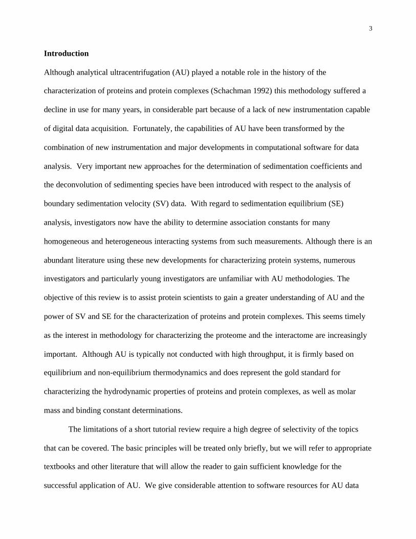
Legends for the Figures

Figure 1: SV data of a bovine serum albumin sample. Shown are the concentration versus radius

distributions at different times after start of the sedimentation at 50,000 rpm. Concentration are in

units of fringe displacement in the interference optical system, with corresponds to approximately

0.3 mg/ml per fringe.

Figure 2: Sedimentation coefficient distributions calculated from the data in Figure 1. Shown are

the distribution of Lamm equation solution c(s) (solid line), the apparent sedimentation coefficient

distribution g(s*) (dotted line), and the integral sedimentation coefficient distribution G(s), scaled to

the loading concentration. The differential distributions c(s) and g(s*) are in units of fringes/S, the

integral distribution G(s) is in units of fractional loading concentration. The inset shows a

chromatogram of BSA in size-exclusion HPLC (Toso Haas, TSK-gel Super SW3000, 4.6 mm × 30

cm).

20004000

6000

6.3 6.4 6.5 6.6 6.7 6.8 6.9 7 7.1

0

0.5

1

1.5

2

radius (cm)time (sec)

conc

entr

atio

n

time (sec)radius (cm)

conc

entra

tion

Lebowitz et al., Figure 1

2 4 6 8 10 12 140

2

4

6

8

c(s)

, g*(

s), a

nd G

(s)

s-value (S)

6 8 10 120.0

0.2

0.4

0.6

0.8

1.0

Lebowitz et al., Figure 2

abs

orba

nce

(OD 28

0)

volume (ml)