Embed Size (px)
DESCRIPTION
A step by step procedure to model rf parabolic reflector.
Citation preview
Solved with COMSOL Multiphysics 5.0
Pa r abo l i c R e f l e c t o r An t e nna
Introduction
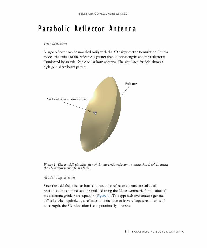
A large reflector can be modeled easily with the 2D axisymmetric formulation. In this model, the radius of the reflector is greater than 20 wavelengths and the reflector is illuminated by an axial feed circular horn antenna. The simulated far-field shows a high-gain sharp beam pattern.
Reflector
Axial feed circular horn antenna
Figure 1: This is a 3D visualization of the parabolic reflector antenna that is solved using the 2D axisymmetric formulation.
Model Definition
Since the axial feed circular horn and parabolic reflector antenna are solids of revolution, the antenna can be simulated using the 2D axisymmetric formulation of the electromagnetic wave equation (Figure 1). This approach overcomes a general difficulty when optimizing a reflector antenna: due to its very large size in terms of wavelength, the 3D calculation is computationally intensive.
1 | P A R A B O L I C R E F L E C T O R A N T E N N A
Solved with COMSOL Multiphysics 5.0
2 | P A R A
In this example, all metal surfaces are modeled as perfect electric conductors (PECs) and all domains are filled with air.
The radius of the circular horn feed waveguide is 0.01 m and the cutoff frequency of the TE11 mode is approximately 8.8 GHz. The operating frequency of the antenna should be higher than the cutoff frequency. The horn aperture radius is 0.03 m and the overall horn length is 0.06 m. A slit-conditioned circular port is assigned on the end of the waveguide to excite the antenna with the TE1m mode. The azimuthal mode number, m, is defined from the physics interface Electromagnetic Waves, Frequency Domain. In this model, m = 1.
The reflector is built using a 53 degree sector of a circle with a radius of 0.85 m. The reflector body is removed from the model domain and, consequently, the PEC is automatically applied to its boundary. The model domain is enclosed by perfectly matched layers (PMLs). The PMLs are thicker than that of other antenna examples in the Model Library since high gain and stronger propagation are expected from the reflector.
A Free Triangular mesh is used for the antenna and air domains. The maximum element size is one-fifth of the wavelength at the simulation frequency. A mapped mesh with 10 layers is used for the PMLs.
Results and Discussion
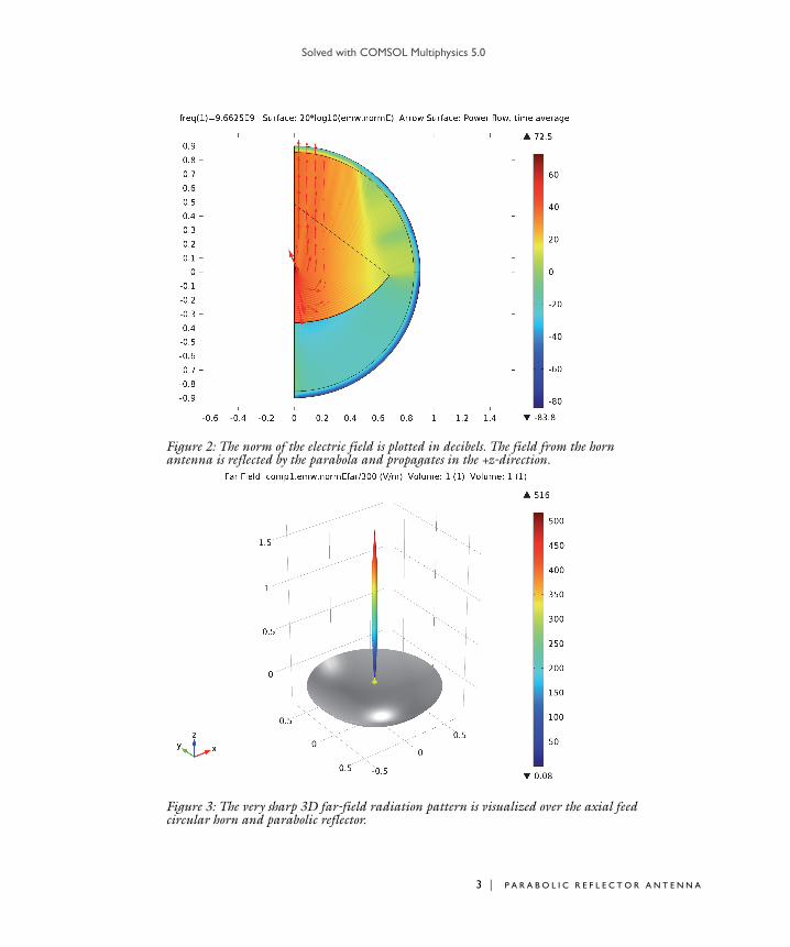
In Figure 2, the norm of the electric field is plotted in decibels with arrows indicating the direction and relative magnitude of power flow. The field from the horn antenna is reflected by the parabola and propagates in the +z-direction, confined near the axis of rotation.
The 3D far-field radiation pattern is plotted with a visualization of the antenna body in Figure 3. The low gain radiation from the axial feed horn results in a very high gain pattern created by the reflector.
B O L I C R E F L E C T O R A N T E N N A
Solved with COMSOL Multiphysics 5.0
Figure 2: The norm of the electric field is plotted in decibels. The field from the horn antenna is reflected by the parabola and propagates in the +z-direction.
Figure 3: The very sharp 3D far-field radiation pattern is visualized over the axial feed circular horn and parabolic reflector.
3 | P A R A B O L I C R E F L E C T O R A N T E N N A

Solved with COMSOL Multiphysics 5.0
4 | P A R
Model Library path: RF_Module/Antennas/parabolic_reflector
Modeling Instructions
From the File menu, choose New.
N E W
1 In the New window, click Model Wizard.
M O D E L W I Z A R D
1 In the Model Wizard window, click 2D Axisymmetric.
2 In the Select physics tree, select Radio Frequency>Electromagnetic Waves, Frequency
Domain (emw).
3 Click Add.
4 Click Study.
5 In the Select study tree, select Preset Studies>Frequency Domain.
6 Click Done.
D E F I N I T I O N S
Parameters1 On the Model toolbar, click Parameters.
2 In the Settings window for Parameters, locate the Parameters section.
A B O L I C R E F L E C T O R A N T E N N A
Solved with COMSOL Multiphysics 5.0
3 In the table, enter the following settings:
Here, c_const is a predefined COMSOL constant for the speed of light in vacuum.
G E O M E T R Y 1
Rectangle 1 (r1)1 On the Geometry toolbar, click Primitives and choose Rectangle.
2 In the Settings window for Rectangle, locate the Size section.
3 In the Width text field, type r1.
4 In the Height text field, type 0.06.
Rectangle 2 (r2)1 On the Geometry toolbar, click Primitives and choose Rectangle.
2 In the Settings window for Rectangle, locate the Size section.
3 In the Width text field, type r1*3.
4 In the Height text field, type l_horn.
Polygon 1 (pol1)1 On the Geometry toolbar, click Primitives and choose Polygon.
2 In the Settings window for Polygon, locate the Coordinates section.
3 In the r text field, type 0.01, 0.03.
4 In the z text field, type l_horn, 0.
5 Click the Build Selected button.
Circle 1 (c1)1 On the Geometry toolbar, click Primitives and choose Circle.
2 In the Settings window for Circle, locate the Size and Shape section.
NAME EXPRESSION VALUE DESCRIPTION
r0 0.85[m] 0.85000 m Reflector, radius
r1 0.01[m] 0.010000 m Feed horn waveguide, radius
fc (1.841*c_const/2/pi/r1)
8.7840E9 1/s Feed horn waveguide, cutoff frequency
f0 fc*1.1 9.6625E9 1/s Frequency
lda0 c_const/f0 0.031027 m Wavelength
l_horn 0.028[m] 0.028000 m Horn length
5 | P A R A B O L I C R E F L E C T O R A N T E N N A

Solved with COMSOL Multiphysics 5.0
6 | P A R
3 In the Radius text field, type 0.9.
4 In the Sector angle text field, type 180.
5 Locate the Rotation Angle section. In the Rotation text field, type 270.
6 Click to expand the Layers section. In the table, enter the following settings:
7 Click the Build Selected button.
8 Click the Zoom Extents button on the Graphics toolbar.
Circle 2 (c2)1 On the Geometry toolbar, click Primitives and choose Circle.
2 In the Settings window for Circle, locate the Size and Shape section.
3 In the Radius text field, type r0.
4 In the Sector angle text field, type 53.
5 Locate the Position section. In the r text field, type 0.
6 In the z text field, type r0-0.365.
7 Locate the Rotation Angle section. In the Rotation text field, type 270.
8 Locate the Layers section. In the table, enter the following settings:
LAYER NAME THICKNESS (M)
Layer 1 1.5*lda0
LAYER NAME THICKNESS (M)
Layer 1 0.002
A B O L I C R E F L E C T O R A N T E N N A
Solved with COMSOL Multiphysics 5.0
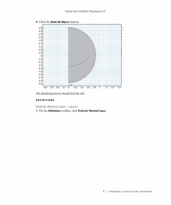
9 Click the Build All Objects button.
The finished geometry should look like this.
D E F I N I T I O N S
Perfectly Matched Layer 1 (pml1)1 On the Definitions toolbar, click Perfectly Matched Layer.
7 | P A R A B O L I C R E F L E C T O R A N T E N N A
Solved with COMSOL Multiphysics 5.0
8 | P A R
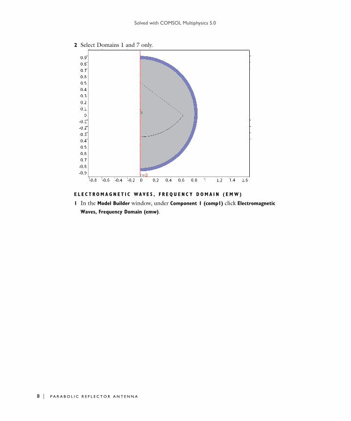
2 Select Domains 1 and 7 only.
E L E C T R O M A G N E T I C WA V E S , F R E Q U E N C Y D O M A I N ( E M W )
1 In the Model Builder window, under Component 1 (comp1) click Electromagnetic
Waves, Frequency Domain (emw).
A B O L I C R E F L E C T O R A N T E N N A
Solved with COMSOL Multiphysics 5.0
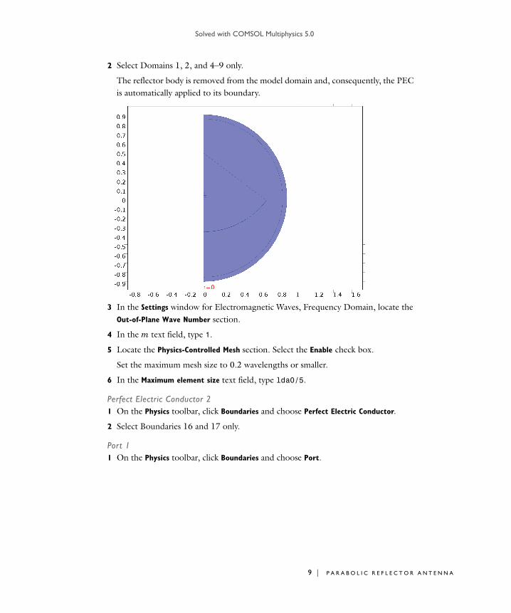
2 Select Domains 1, 2, and 4–9 only.
The reflector body is removed from the model domain and, consequently, the PEC is automatically applied to its boundary.
3 In the Settings window for Electromagnetic Waves, Frequency Domain, locate the Out-of-Plane Wave Number section.
4 In the m text field, type 1.
5 Locate the Physics-Controlled Mesh section. Select the Enable check box.
Set the maximum mesh size to 0.2 wavelengths or smaller.
6 In the Maximum element size text field, type lda0/5.
Perfect Electric Conductor 21 On the Physics toolbar, click Boundaries and choose Perfect Electric Conductor.
2 Select Boundaries 16 and 17 only.
Port 11 On the Physics toolbar, click Boundaries and choose Port.
9 | P A R A B O L I C R E F L E C T O R A N T E N N A
Solved with COMSOL Multiphysics 5.0
10 | P A
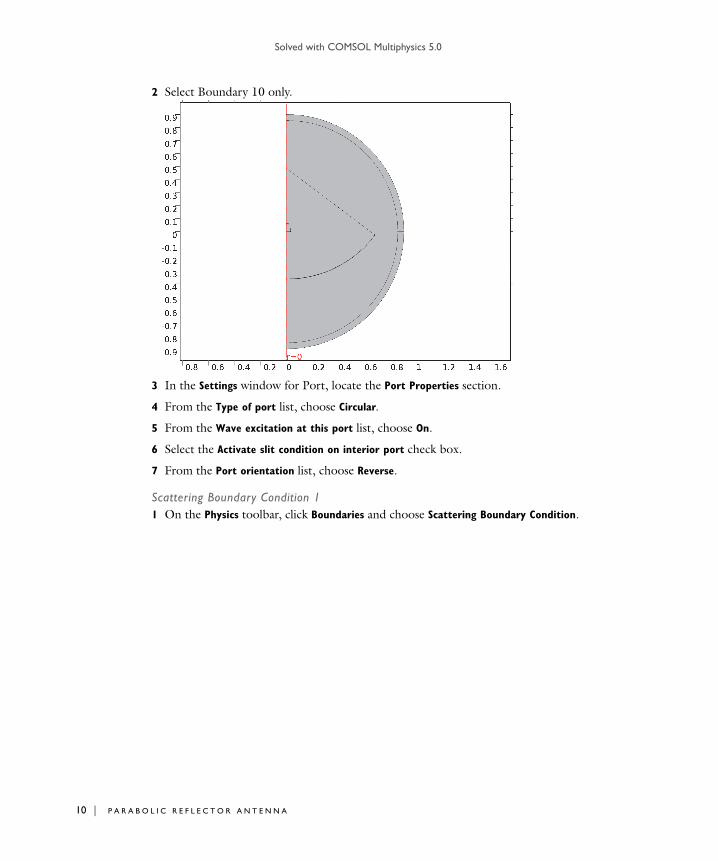
2 Select Boundary 10 only.
3 In the Settings window for Port, locate the Port Properties section.
4 From the Type of port list, choose Circular.
5 From the Wave excitation at this port list, choose On.
6 Select the Activate slit condition on interior port check box.
7 From the Port orientation list, choose Reverse.
Scattering Boundary Condition 11 On the Physics toolbar, click Boundaries and choose Scattering Boundary Condition.
R A B O L I C R E F L E C T O R A N T E N N A
Solved with COMSOL Multiphysics 5.0
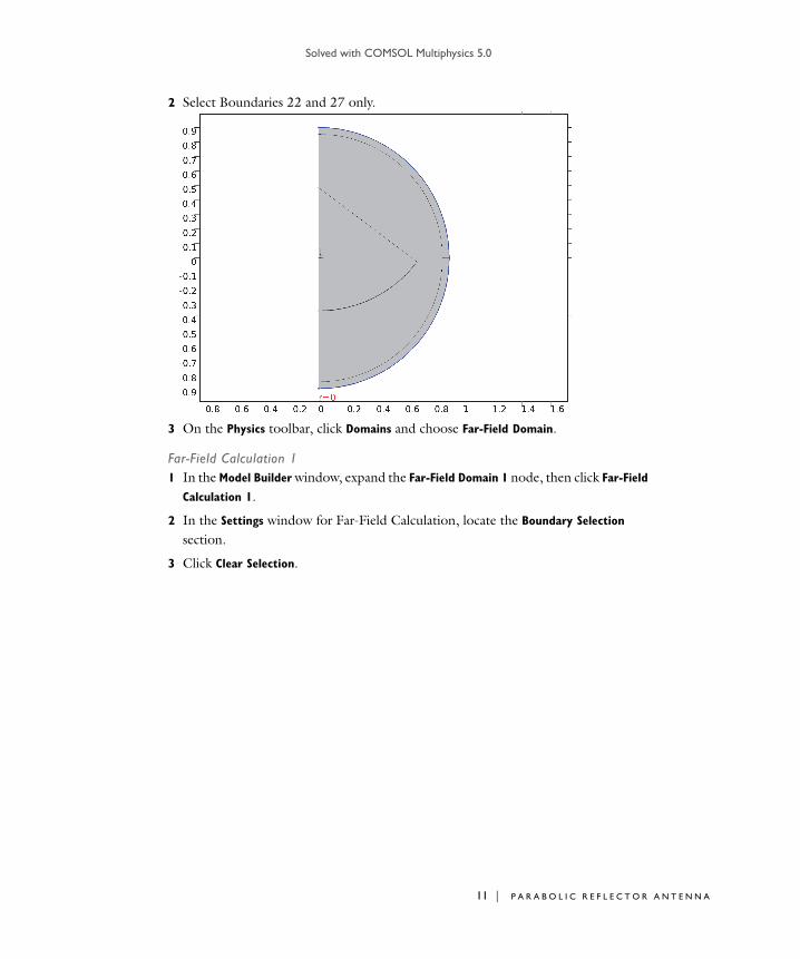
2 Select Boundaries 22 and 27 only.
3 On the Physics toolbar, click Domains and choose Far-Field Domain.
Far-Field Calculation 11 In the Model Builder window, expand the Far-Field Domain 1 node, then click Far-Field
Calculation 1.
2 In the Settings window for Far-Field Calculation, locate the Boundary Selection section.
3 Click Clear Selection.
11 | P A R A B O L I C R E F L E C T O R A N T E N N A
Solved with COMSOL Multiphysics 5.0
12 | P A
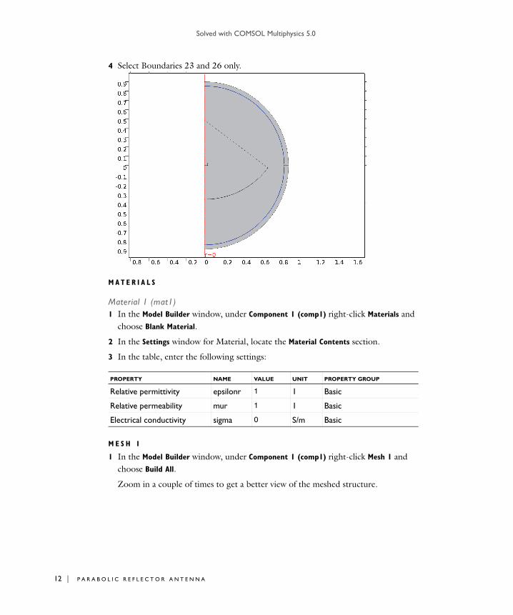
4 Select Boundaries 23 and 26 only.
M A T E R I A L S
Material 1 (mat1)1 In the Model Builder window, under Component 1 (comp1) right-click Materials and
choose Blank Material.
2 In the Settings window for Material, locate the Material Contents section.
3 In the table, enter the following settings:
M E S H 1
1 In the Model Builder window, under Component 1 (comp1) right-click Mesh 1 and choose Build All.
Zoom in a couple of times to get a better view of the meshed structure.
PROPERTY NAME VALUE UNIT PROPERTY GROUP
Relative permittivity epsilonr 1 1 Basic
Relative permeability mur 1 1 Basic
Electrical conductivity sigma 0 S/m Basic
R A B O L I C R E F L E C T O R A N T E N N A
Solved with COMSOL Multiphysics 5.0
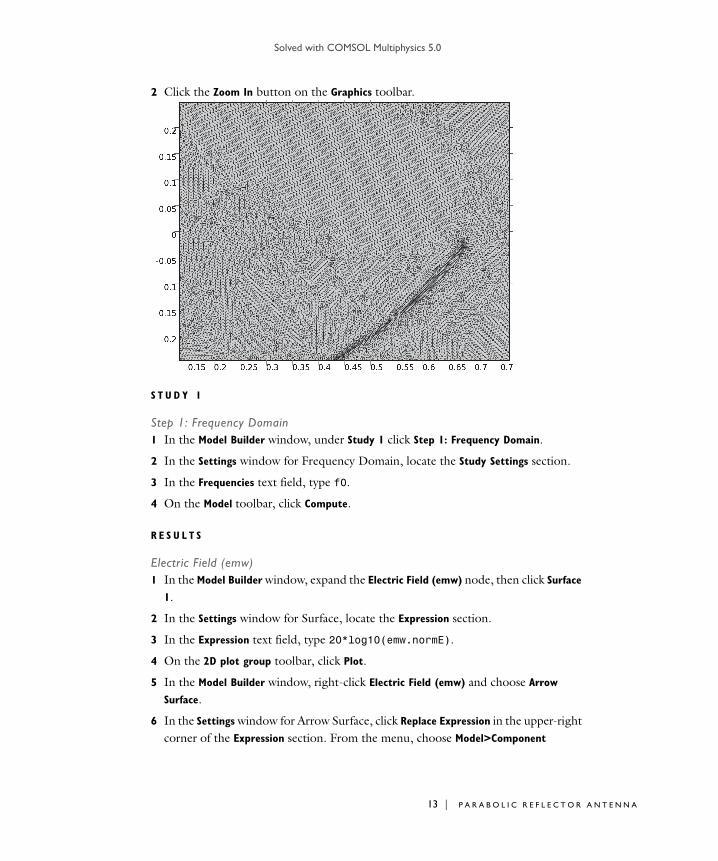
2 Click the Zoom In button on the Graphics toolbar.
S T U D Y 1
Step 1: Frequency Domain1 In the Model Builder window, under Study 1 click Step 1: Frequency Domain.
2 In the Settings window for Frequency Domain, locate the Study Settings section.
3 In the Frequencies text field, type f0.
4 On the Model toolbar, click Compute.
R E S U L T S
Electric Field (emw)1 In the Model Builder window, expand the Electric Field (emw) node, then click Surface
1.
2 In the Settings window for Surface, locate the Expression section.
3 In the Expression text field, type 20*log10(emw.normE).
4 On the 2D plot group toolbar, click Plot.
5 In the Model Builder window, right-click Electric Field (emw) and choose Arrow
Surface.
6 In the Settings window for Arrow Surface, click Replace Expression in the upper-right corner of the Expression section. From the menu, choose Model>Component
13 | P A R A B O L I C R E F L E C T O R A N T E N N A
Solved with COMSOL Multiphysics 5.0
14 | P A
1>Electromagnetic Waves, Frequency Domain>Energy and
power>emw.Poavr,emw.Poavz - Power flow, time average.
7 Locate the Coloring and Style section. From the Arrow length list, choose Logarithmic.
8 Select the Scale factor check box.
9 In the associated text field, type 0.004.
10 On the 2D plot group toolbar, click Plot.
11 Click the Zoom Extents button on the Graphics toolbar.
Compare with the plot in Figure 2.
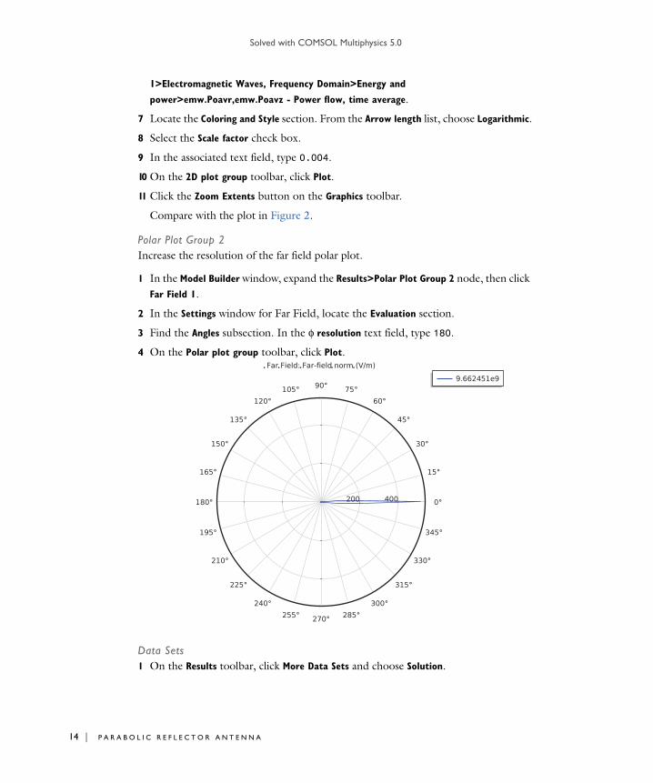
Polar Plot Group 2Increase the resolution of the far field polar plot.
1 In the Model Builder window, expand the Results>Polar Plot Group 2 node, then click Far Field 1.
2 In the Settings window for Far Field, locate the Evaluation section.
3 Find the Angles subsection. In the φ resolution text field, type 180.
4 On the Polar plot group toolbar, click Plot.
Data Sets1 On the Results toolbar, click More Data Sets and choose Solution.
R A B O L I C R E F L E C T O R A N T E N N A

Solved with COMSOL Multiphysics 5.0
2 On the Results toolbar, click Selection.
3 In the Settings window for Selection, locate the Geometric Entity Selection section.
4 From the Geometric entity level list, choose Domain.
5 Select Domains 5, 6, and 8 only.
6 On the Results toolbar, click More Data Sets and choose Revolution 2D.
7 In the Settings window for Revolution 2D, locate the Data section.
8 From the Data set list, choose Study 1/Solution 1 (2).
9 Right-click Results>Data Sets>Revolution 2D 2 and choose Rename.
10 In the Rename Revolution 2D dialog box, type Revolution 2D Feed horn in the New label text field.
11 Click OK.
12 On the Results toolbar, click More Data Sets and choose Solution.
13 On the Results toolbar, click Selection.
14 In the Settings window for Selection, locate the Geometric Entity Selection section.
15 From the Geometric entity level list, choose Domain.
16 Select Domain 3 only.
17 On the Results toolbar, click More Data Sets and choose Revolution 2D.
18 In the Settings window for Revolution 2D, locate the Data section.
19 From the Data set list, choose Study 1/Solution 1 (3).
20 Right-click Results>Data Sets>Revolution 2D 3 and choose Rename.
21 In the Rename Revolution 2D dialog box, type Revolution 2D Reflector in the New label text field.
22 Click OK.
3D Plot Group 31 In the Model Builder window, under Results right-click 3D Plot Group 3 and choose
Surface.
2 In the Settings window for Volume, locate the Data section.
3 From the Data set list, choose Revolution 2D Feed horn.
4 Locate the Expression section. In the Expression text field, type 1.
5 Locate the Coloring and Style section. From the Coloring list, choose Uniform.
6 From the Color list, choose Yellow.
7 In the Model Builder window, right-click 3D Plot Group 3 and choose Surface.
15 | P A R A B O L I C R E F L E C T O R A N T E N N A

Solved with COMSOL Multiphysics 5.0
16 | P A
8 In the Settings window for Volume, locate the Data section.
9 From the Data set list, choose Revolution 2D Reflector.
10 Locate the Expression section. In the Expression text field, type 1.
11 Locate the Coloring and Style section. From the Coloring list, choose Uniform.
12 From the Color list, choose Gray.
13 In the Model Builder window, under Results>3D Plot Group 3 click Far Field 1.
14 In the Settings window for Far Field, locate the Expression section.
15 In the Expression text field, type comp1.emw.normEfar/300.
16 On the 3D plot group toolbar, click Plot.
17 Click the Zoom Extents button on the Graphics toolbar.
The plotted figure describes the axial feed circular horn and parabolic reflector as well as the 3D far-field pattern as shown in Figure 3.
R A B O L I C R E F L E C T O R A N T E N N A