Embed Size (px)
DESCRIPTION
Models.heat.Friction Stir Welding
Citation preview
Solved with COMSOL Multiphysics 4.3b
© 2 0 1 3 C O
F r i c t i o n S t i r We l d i n g
Introduction
Manufacturers use a modern welding method called friction stir welding to join aluminum plates. This model analyzes the heat transfer in this welding process. The model is based on a paper by M. Song and R. Kovacevic (Ref. 1).
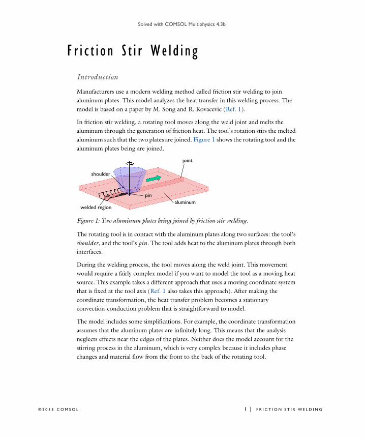
In friction stir welding, a rotating tool moves along the weld joint and melts the aluminum through the generation of friction heat. The tool’s rotation stirs the melted aluminum such that the two plates are joined. Figure 1 shows the rotating tool and the aluminum plates being are joined.
aluminum
shoulder
pin
welded region
joint
Figure 1: Two aluminum plates being joined by friction stir welding.
The rotating tool is in contact with the aluminum plates along two surfaces: the tool’s shoulder, and the tool’s pin. The tool adds heat to the aluminum plates through both interfaces.
During the welding process, the tool moves along the weld joint. This movement would require a fairly complex model if you want to model the tool as a moving heat source. This example takes a different approach that uses a moving coordinate system that is fixed at the tool axis (Ref. 1 also takes this approach). After making the coordinate transformation, the heat transfer problem becomes a stationary convection-conduction problem that is straightforward to model.
The model includes some simplifications. For example, the coordinate transformation assumes that the aluminum plates are infinitely long. This means that the analysis neglects effects near the edges of the plates. Neither does the model account for the stirring process in the aluminum, which is very complex because it includes phase changes and material flow from the front to the back of the rotating tool.
M S O L 1 | F R I C T I O N S T I R W E L D I N G
Solved with COMSOL Multiphysics 4.3b
2 | F R I C
Model Definition
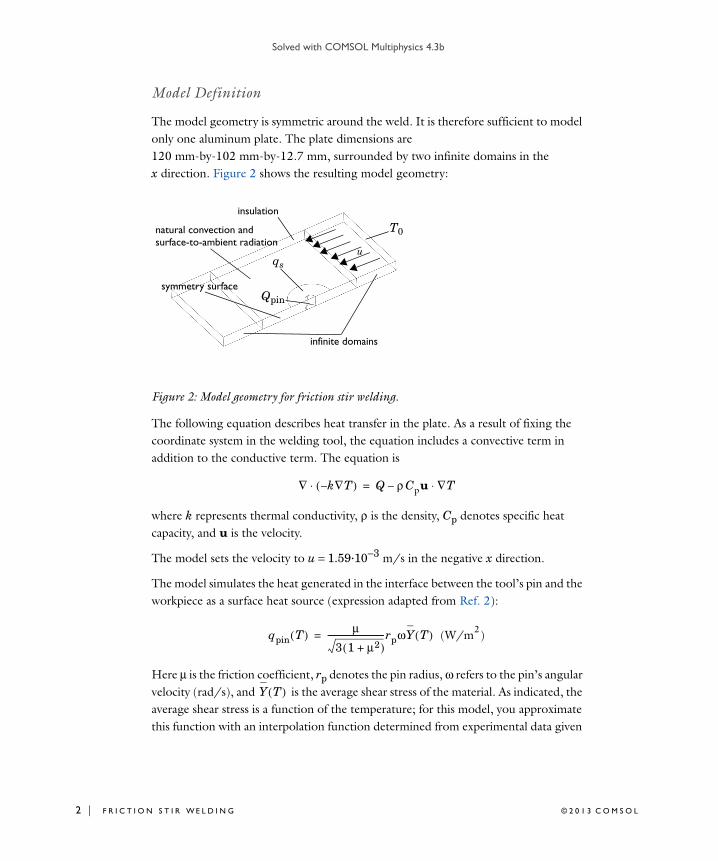
The model geometry is symmetric around the weld. It is therefore sufficient to model only one aluminum plate. The plate dimensions are 120 mm-by-102 mm-by-12.7 mm, surrounded by two infinite domains in the x direction. Figure 2 shows the resulting model geometry:
qs
Qpin
u
T0
insulation
symmetry surface
natural convection and surface-to-ambient radiation
infinite domains
Figure 2: Model geometry for friction stir welding.
The following equation describes heat transfer in the plate. As a result of fixing the coordinate system in the welding tool, the equation includes a convective term in addition to the conductive term. The equation is
where k represents thermal conductivity, ρ is the density, Cp denotes specific heat capacity, and u is the velocity.
The model sets the velocity to u = 1.59·10−3 m/s in the negative x direction.
The model simulates the heat generated in the interface between the tool’s pin and the workpiece as a surface heat source (expression adapted from Ref. 2):
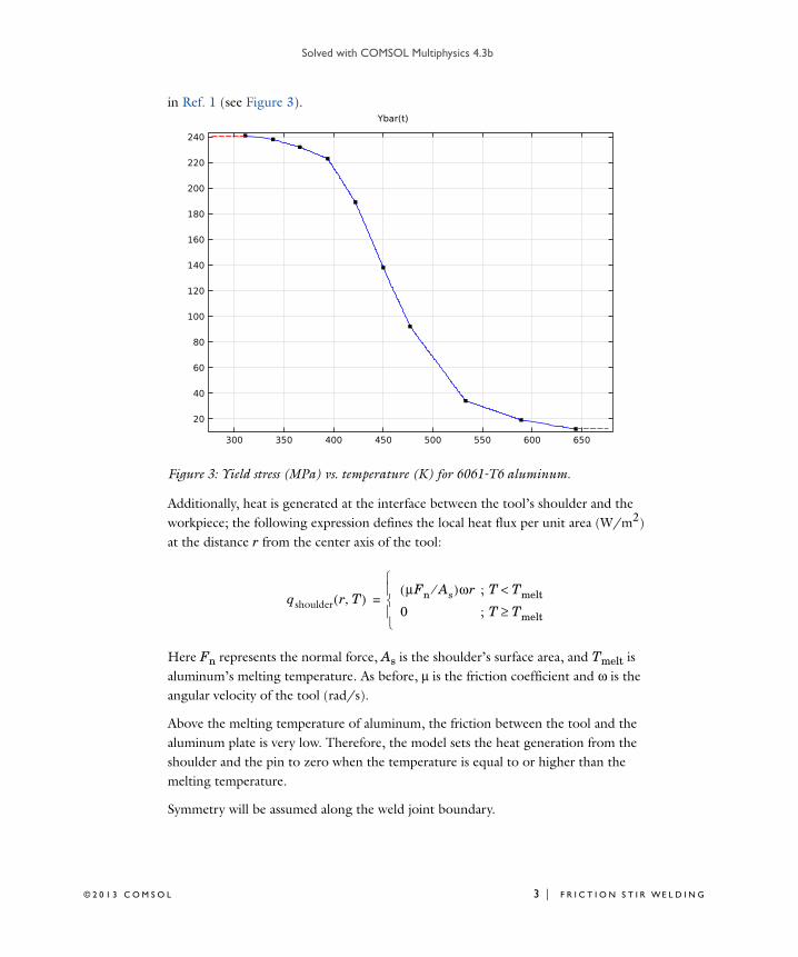
Here μ is the friction coefficient, rp denotes the pin radius, ω refers to the pin’s angular velocity (rad/s), and Y T( ) is the average shear stress of the material. As indicated, the average shear stress is a function of the temperature; for this model, you approximate this function with an interpolation function determined from experimental data given
∇ k∇T–( )⋅ Q ρ Cpu ∇T⋅–=
qpin T( ) μ3 1 μ2+( )----------------------------rpωY T( ) (W/m2)=
T I O N S T I R W E L D I N G © 2 0 1 3 C O M S O L
Solved with COMSOL Multiphysics 4.3b
© 2 0 1 3 C O
in Ref. 1 (see Figure 3).
Figure 3: Yield stress (MPa) vs. temperature (K) for 6061-T6 aluminum.
Additionally, heat is generated at the interface between the tool’s shoulder and the workpiece; the following expression defines the local heat flux per unit area (W/m2) at the distance r from the center axis of the tool:
Here Fn represents the normal force, As is the shoulder’s surface area, and Tmelt is aluminum’s melting temperature. As before, μ is the friction coefficient and ω is the angular velocity of the tool (rad/s).
Above the melting temperature of aluminum, the friction between the tool and the aluminum plate is very low. Therefore, the model sets the heat generation from the shoulder and the pin to zero when the temperature is equal to or higher than the melting temperature.
Symmetry will be assumed along the weld joint boundary.
qshoulder r T,( )μFn As⁄( )ωr ; T Tmelt<
0 ; T Tmelt≥
=
M S O L 3 | F R I C T I O N S T I R W E L D I N G
Solved with COMSOL Multiphysics 4.3b
4 | F R I C
The upper and lower surfaces of the aluminum plates lose heat due to natural convection and surface-to-ambient radiation. The corresponding heat flux expressions for these surfaces are
where hup and hdown are heat transfer coefficients for natural convection, T0 is an associated reference temperature, ε is the surface emissivity, σ is the Stefan-Boltzmann constant, and Tamb is the ambient air temperature.
The modeling of an infinite domain on the left-hand side, where the aluminum leaves the computational domain, makes sure that the temperature is in equilibrium with the temperature at infinity through natural convection and surface-to-ambient radiation. You therefore set the boundary condition to insulation at that location.
You can compute values for the heat transfer coefficients using empirical expressions available in the heat-transfer literature, for example, Ref. 3. In this model, use the values hup = 12.25 W/(m2·K) and hdown = 6.25 W/(m2·K)
qup hup T0 T–( ) εσ Tamb4 T4
–( )+=
qdown hdown T0 T–( ) εσ Tamb4 T4
–( )+=
T I O N S T I R W E L D I N G © 2 0 1 3 C O M S O L
Solved with COMSOL Multiphysics 4.3b
© 2 0 1 3 C O
Results and Discussion
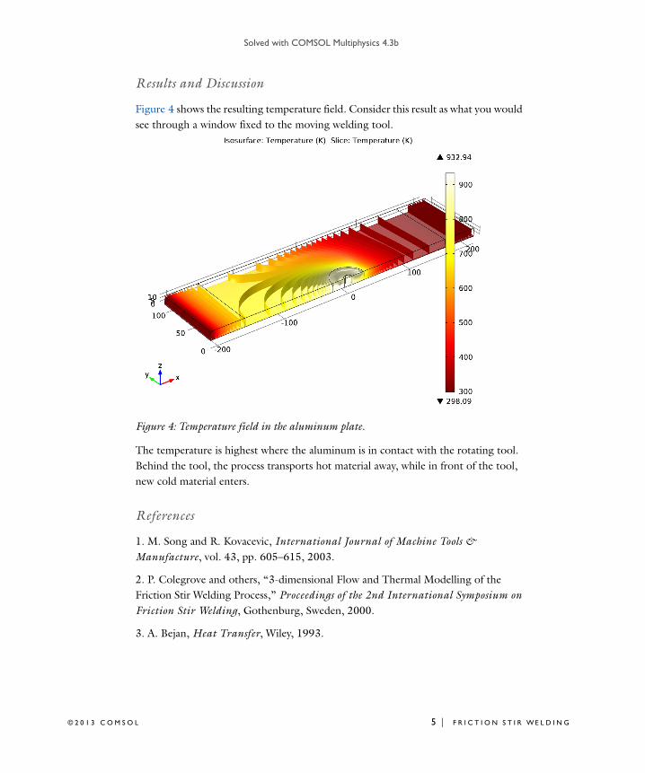
Figure 4 shows the resulting temperature field. Consider this result as what you would see through a window fixed to the moving welding tool.
Figure 4: Temperature field in the aluminum plate.
The temperature is highest where the aluminum is in contact with the rotating tool. Behind the tool, the process transports hot material away, while in front of the tool, new cold material enters.
References
1. M. Song and R. Kovacevic, International Journal of Machine Tools & Manufacture, vol. 43, pp. 605–615, 2003.
2. P. Colegrove and others, “3-dimensional Flow and Thermal Modelling of the Friction Stir Welding Process,” Proceedings of the 2nd International Symposium on Friction Stir Welding, Gothenburg, Sweden, 2000.
3. A. Bejan, Heat Transfer, Wiley, 1993.
M S O L 5 | F R I C T I O N S T I R W E L D I N G
Solved with COMSOL Multiphysics 4.3b
6 | F R I C
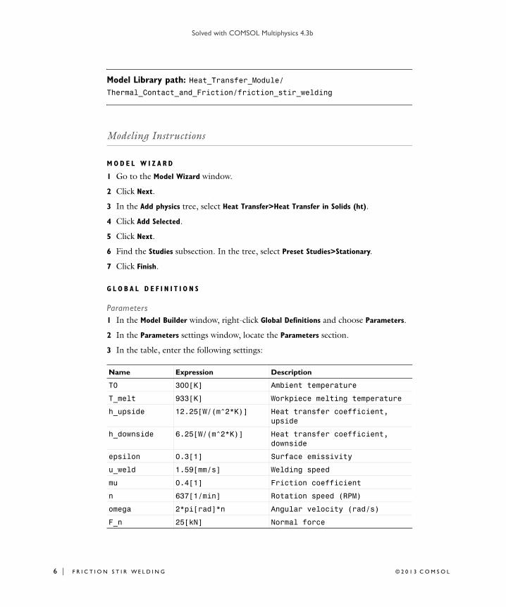
Model Library path: Heat_Transfer_Module/Thermal_Contact_and_Friction/friction_stir_welding
Modeling Instructions
M O D E L W I Z A R D
1 Go to the Model Wizard window.
2 Click Next.
3 In the Add physics tree, select Heat Transfer>Heat Transfer in Solids (ht).
4 Click Add Selected.
5 Click Next.
6 Find the Studies subsection. In the tree, select Preset Studies>Stationary.
7 Click Finish.
G L O B A L D E F I N I T I O N S
Parameters1 In the Model Builder window, right-click Global Definitions and choose Parameters.
2 In the Parameters settings window, locate the Parameters section.
3 In the table, enter the following settings:
Name Expression Description
T0 300[K] Ambient temperature
T_melt 933[K] Workpiece melting temperature
h_upside 12.25[W/(m^2*K)] Heat transfer coefficient, upside
h_downside 6.25[W/(m^2*K)] Heat transfer coefficient, downside
epsilon 0.3[1] Surface emissivity
u_weld 1.59[mm/s] Welding speed
mu 0.4[1] Friction coefficient
n 637[1/min] Rotation speed (RPM)
omega 2*pi[rad]*n Angular velocity (rad/s)
F_n 25[kN] Normal force
T I O N S T I R W E L D I N G © 2 0 1 3 C O M S O L

Solved with COMSOL Multiphysics 4.3b
© 2 0 1 3 C O
Interpolation 11 Right-click Global Definitions and choose Functions>Interpolation.
2 In the Interpolation settings window, locate the Definition section.
3 In the Function name edit field, type Ybar.
4 In the table, enter the following settings:
5 Click the Plot button.
If you have entered the numbers correctly, the curve should look like that in Figure 3.
Step 11 Right-click Global Definitions and choose Functions>Step.
2 In the Step settings window, click to expand the Smoothing section.
3 In the Size of transition zone edit field, type 5.
G E O M E T R Y 1
1 In the Model Builder window, under Model 1 click Geometry 1.
2 In the Geometry settings window, locate the Units section.
3 From the Length unit list, choose mm.
r_pin 6[mm] Pin radius
r_shoulder 25[mm] Shoulder radius
A_s pi*(r_shoulder^2-r_pin^2)
Shoulder surface area
t f(t)
311 241
339 238
366 232
394 223
422 189
450 138
477 92
533 34
589 19
644 12
Name Expression Description
M S O L 7 | F R I C T I O N S T I R W E L D I N G

Solved with COMSOL Multiphysics 4.3b
8 | F R I C
Block 11 Right-click Model 1>Geometry 1 and choose Block.
2 In the Block settings window, locate the Size and Shape section.
3 In the Width edit field, type 320.
4 In the Depth edit field, type 102.
5 In the Height edit field, type 12.7.
6 Locate the Position section. In the x edit field, type -160.
7 Click the Build Selected button.
Block 21 In the Model Builder window, right-click Geometry 1 and choose Block.
2 In the Block settings window, locate the Size and Shape section.
3 In the Width edit field, type 420.
4 In the Depth edit field, type 102.
5 In the Height edit field, type 12.7.
6 Locate the Position section. In the x edit field, type -210.
7 Click the Build Selected button.
Cylinder 11 Right-click Geometry 1 and choose Cylinder.
2 In the Cylinder settings window, locate the Size and Shape section.
3 In the Radius edit field, type r_shoulder.
4 In the Height edit field, type 12.7.
5 Click the Build Selected button.
Cylinder 21 Right-click Geometry 1 and choose Cylinder.
2 In the Cylinder settings window, locate the Size and Shape section.
3 In the Radius edit field, type r_pin.
4 In the Height edit field, type 12.7.
5 Click the Build Selected button.
Block 31 Right-click Geometry 1 and choose Block.
2 In the Block settings window, locate the Size and Shape section.
T I O N S T I R W E L D I N G © 2 0 1 3 C O M S O L

Solved with COMSOL Multiphysics 4.3b
© 2 0 1 3 C O
3 In the Width edit field, type 2*r_shoulder.
4 In the Depth edit field, type r_shoulder.
5 In the Height edit field, type 12.7.
6 Locate the Position section. In the x edit field, type -r_shoulder.
7 In the y edit field, type -r_shoulder.
8 Click the Build Selected button.
Difference 11 Right-click Geometry 1 and choose Boolean Operations>Difference.
2 In the Difference settings window, locate the Difference section.
3 Under Objects to add, click Activate Selection.
4 Select the objects cyl1 and cyl2 only.
5 Under Objects to subtract, click Activate Selection.
6 Select the object blk3 only.
7 Click the Build Selected button.
Form Union1 In the Model Builder window, under Model 1>Geometry 1 right-click Form Union and
choose Build Selected.
The model geometry is now complete.
M S O L 9 | F R I C T I O N S T I R W E L D I N G
Solved with COMSOL Multiphysics 4.3b
10 | F R I
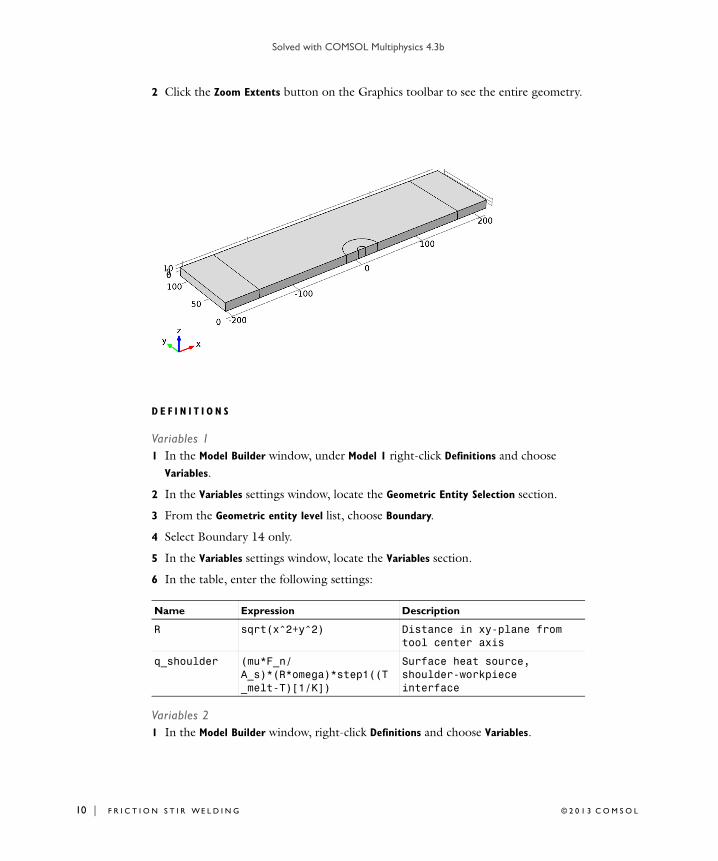
2 Click the Zoom Extents button on the Graphics toolbar to see the entire geometry.
D E F I N I T I O N S
Variables 11 In the Model Builder window, under Model 1 right-click Definitions and choose
Variables.
2 In the Variables settings window, locate the Geometric Entity Selection section.
3 From the Geometric entity level list, choose Boundary.
4 Select Boundary 14 only.
5 In the Variables settings window, locate the Variables section.
6 In the table, enter the following settings:
Variables 21 In the Model Builder window, right-click Definitions and choose Variables.
Name Expression Description
R sqrt(x^2+y^2) Distance in xy-plane from tool center axis
q_shoulder (mu*F_n/A_s)*(R*omega)*step1((T_melt-T)[1/K])
Surface heat source, shoulder-workpiece interface
C T I O N S T I R W E L D I N G © 2 0 1 3 C O M S O L
Solved with COMSOL Multiphysics 4.3b
© 2 0 1 3 C O
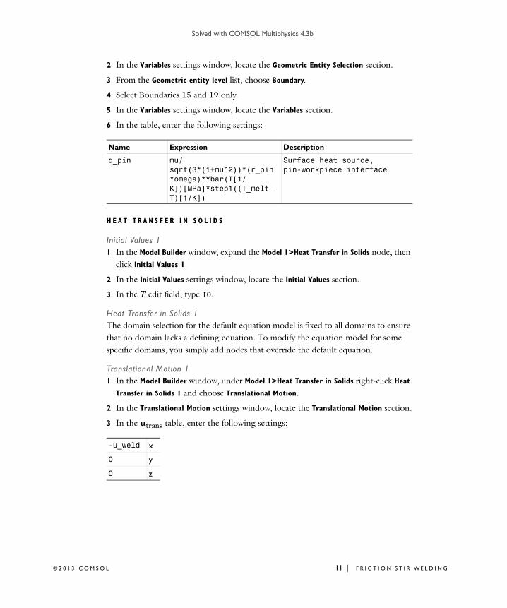
2 In the Variables settings window, locate the Geometric Entity Selection section.
3 From the Geometric entity level list, choose Boundary.
4 Select Boundaries 15 and 19 only.
5 In the Variables settings window, locate the Variables section.
6 In the table, enter the following settings:
H E A T TR A N S F E R I N S O L I D S
Initial Values 11 In the Model Builder window, expand the Model 1>Heat Transfer in Solids node, then
click Initial Values 1.
2 In the Initial Values settings window, locate the Initial Values section.
3 In the T edit field, type T0.
Heat Transfer in Solids 1The domain selection for the default equation model is fixed to all domains to ensure that no domain lacks a defining equation. To modify the equation model for some specific domains, you simply add nodes that override the default equation.
Translational Motion 11 In the Model Builder window, under Model 1>Heat Transfer in Solids right-click Heat
Transfer in Solids 1 and choose Translational Motion.
2 In the Translational Motion settings window, locate the Translational Motion section.
3 In the utrans table, enter the following settings:
Name Expression Description
q_pin mu/sqrt(3*(1+mu^2))*(r_pin*omega)*Ybar(T[1/K])[MPa]*step1((T_melt-T)[1/K])
Surface heat source, pin-workpiece interface
-u_weld x
0 y
0 z
M S O L 11 | F R I C T I O N S T I R W E L D I N G
Solved with COMSOL Multiphysics 4.3b
12 | F R I
D E F I N I T I O N S
Infinite Element Domain 11 In the Model Builder window, under Model 1 right-click Definitions and choose Infinite
Element Domain.
2 Select Domains 1 and 5 only.
H E A T TR A N S F E R I N S O L I D S
Surface-to-Ambient Radiation 11 In the Model Builder window, under Model 1 right-click Heat Transfer in Solids and
choose Surface-to-Ambient Radiation.
2 Select Boundaries 3, 4, 8, 9, 13, 25, and 26 only.
Together, these boundaries form the top and bottom surfaces of the geometry.
3 In the Surface-to-Ambient Radiation settings window, locate the Surface-to-Ambient
Radiation section.
4 From the ε list, choose User defined. In the associated edit field, type epsilon.
5 In the Tamb edit field, type T0.
Outflow 11 In the Model Builder window, right-click Heat Transfer in Solids and choose Outflow.
2 Select Boundary 1 only.
Heat Flux 11 Right-click Heat Transfer in Solids and choose Heat Flux.
2 Select Boundaries 3, 8, 13, and 25 only.
3 In the Heat Flux settings window, locate the Heat Flux section.
4 Click the Inward heat flux button.
5 In the h edit field, type h_downside.
6 In the Text edit field, type T0.
Heat Flux 21 Right-click Heat Transfer in Solids and choose Heat Flux.
2 Select Boundaries 4, 9, and 26 only.
3 In the Heat Flux settings window, locate the Heat Flux section.
4 Click the Inward heat flux button.
5 In the h edit field, type h_upside.
C T I O N S T I R W E L D I N G © 2 0 1 3 C O M S O L

Solved with COMSOL Multiphysics 4.3b
© 2 0 1 3 C O
6 In the Text edit field, type T0.
Heat Flux 31 Right-click Heat Transfer in Solids and choose Heat Flux.
2 Select Boundary 14 only.
3 In the Heat Flux settings window, locate the Heat Flux section.
4 In the q0 edit field, type q_shoulder.
Boundary Heat Source 11 Right-click Heat Transfer in Solids and choose Boundary Heat Source.
2 Select Boundaries 15 and 19 only.
3 In the Boundary Heat Source settings window, locate the Boundary Heat Source section.
4 In the Qb edit field, type q_pin.
Temperature 11 Right-click Heat Transfer in Solids and choose Temperature.
2 Select Boundary 28 only.
3 In the Temperature settings window, locate the Temperature section.
4 In the T0 edit field, type T0.
M A T E R I A L S
Now specify the materials. By default, the first material you add applies to all domains. To specify a different material in some domains you simply add another material for those domains.
Material Browser1 In the Model Builder window, under Model 1 right-click Materials and choose Open
Material Browser.
2 In the Material Browser settings window, In the tree, select Built-In>Aluminum.
3 Click Add Material to Model.
Add a material for the pin and specify the required properties.
Material 21 In the Model Builder window, right-click Materials and choose Material.
2 Right-click Material 2 and choose Rename.
3 Go to the Rename Material dialog box and type Pin in the New name edit field.
M S O L 13 | F R I C T I O N S T I R W E L D I N G
Solved with COMSOL Multiphysics 4.3b
14 | F R I
4 Click OK.
5 Select Domain 4 only.
6 In the Material settings window, locate the Material Contents section.
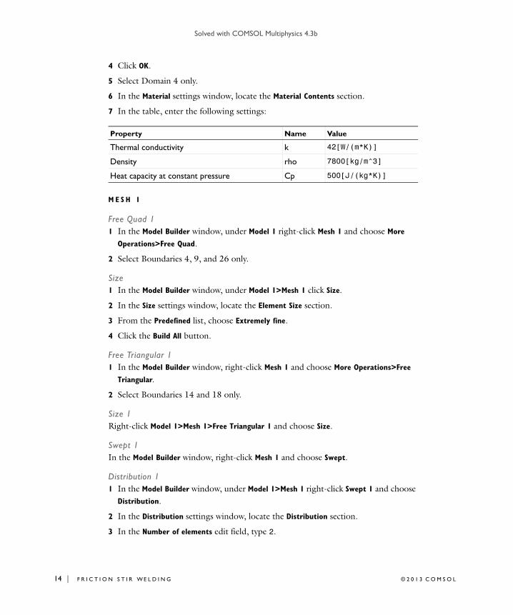
7 In the table, enter the following settings:
M E S H 1
Free Quad 11 In the Model Builder window, under Model 1 right-click Mesh 1 and choose More
Operations>Free Quad.
2 Select Boundaries 4, 9, and 26 only.
Size1 In the Model Builder window, under Model 1>Mesh 1 click Size.
2 In the Size settings window, locate the Element Size section.
3 From the Predefined list, choose Extremely fine.
4 Click the Build All button.
Free Triangular 11 In the Model Builder window, right-click Mesh 1 and choose More Operations>Free
Triangular.
2 Select Boundaries 14 and 18 only.
Size 1Right-click Model 1>Mesh 1>Free Triangular 1 and choose Size.
Swept 1In the Model Builder window, right-click Mesh 1 and choose Swept.
Distribution 11 In the Model Builder window, under Model 1>Mesh 1 right-click Swept 1 and choose
Distribution.
2 In the Distribution settings window, locate the Distribution section.
3 In the Number of elements edit field, type 2.
Property Name Value
Thermal conductivity k 42[W/(m*K)]
Density rho 7800[kg/m^3]
Heat capacity at constant pressure Cp 500[J/(kg*K)]
C T I O N S T I R W E L D I N G © 2 0 1 3 C O M S O L
Solved with COMSOL Multiphysics 4.3b
© 2 0 1 3 C O
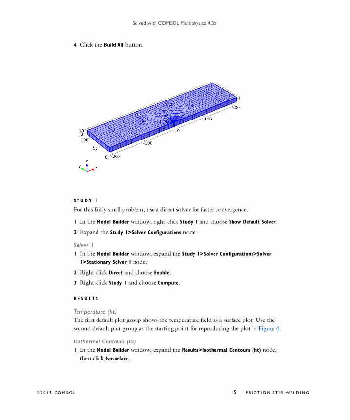
4 Click the Build All button.
S T U D Y 1
For this fairly small problem, use a direct solver for faster convergence.
1 In the Model Builder window, right-click Study 1 and choose Show Default Solver.
2 Expand the Study 1>Solver Configurations node.
Solver 11 In the Model Builder window, expand the Study 1>Solver Configurations>Solver
1>Stationary Solver 1 node.
2 Right-click Direct and choose Enable.
3 Right-click Study 1 and choose Compute.
R E S U L T S
Temperature (ht)The first default plot group shows the temperature field as a surface plot. Use the second default plot group as the starting point for reproducing the plot in Figure 4.
Isothermal Contours (ht)1 In the Model Builder window, expand the Results>Isothermal Contours (ht) node,
then click Isosurface.
M S O L 15 | F R I C T I O N S T I R W E L D I N G

Solved with COMSOL Multiphysics 4.3b
16 | F R I
2 In the Isosurface settings window, locate the Levels section.
3 From the Entry method list, choose Levels.
4 In the Levels edit field, type range(300,20,980).
5 Locate the Coloring and Style section. Clear the Color legend check box.
6 In the Model Builder window, under Results>Isothermal Contours (ht) right-click Arrow volume and choose Disable.
7 Right-click Isothermal Contours (ht) and choose Slice.
8 In the Slice settings window, locate the Plane Data section.
9 From the Plane list, choose xy-planes.
10 From the Entry method list, choose Coordinates.
11 In the z-coordinates edit field, type 1.
12 Locate the Coloring and Style section. From the Color table list, choose ThermalLight.
13 Click the Plot button.
C T I O N S T I R W E L D I N G © 2 0 1 3 C O M S O L