1

Models of the Solar Wind Interaction with Local Interstellar Cloud

V. V. Izmodenova

aDivision of Aeromechanics and Gas Dynamics, Department of Mechanics andMathematics, Lomonosov Moscow State University, Moscow, 119899, Russia

This paper reviews the theoretical approaches and existing models of the solar windinteraction with the Local Interstellar Cloud (LIC). Models discussed take into accountthe multi-component nature of the solar wind and local interstellar medium. Basic resultsof the modeling and their possible applications to interpretation of space experiments aresummarized. Open questions of global modeling of the solar wind/LIC interaction andfuture perspectives are discussed.

1. INTRODUCTION

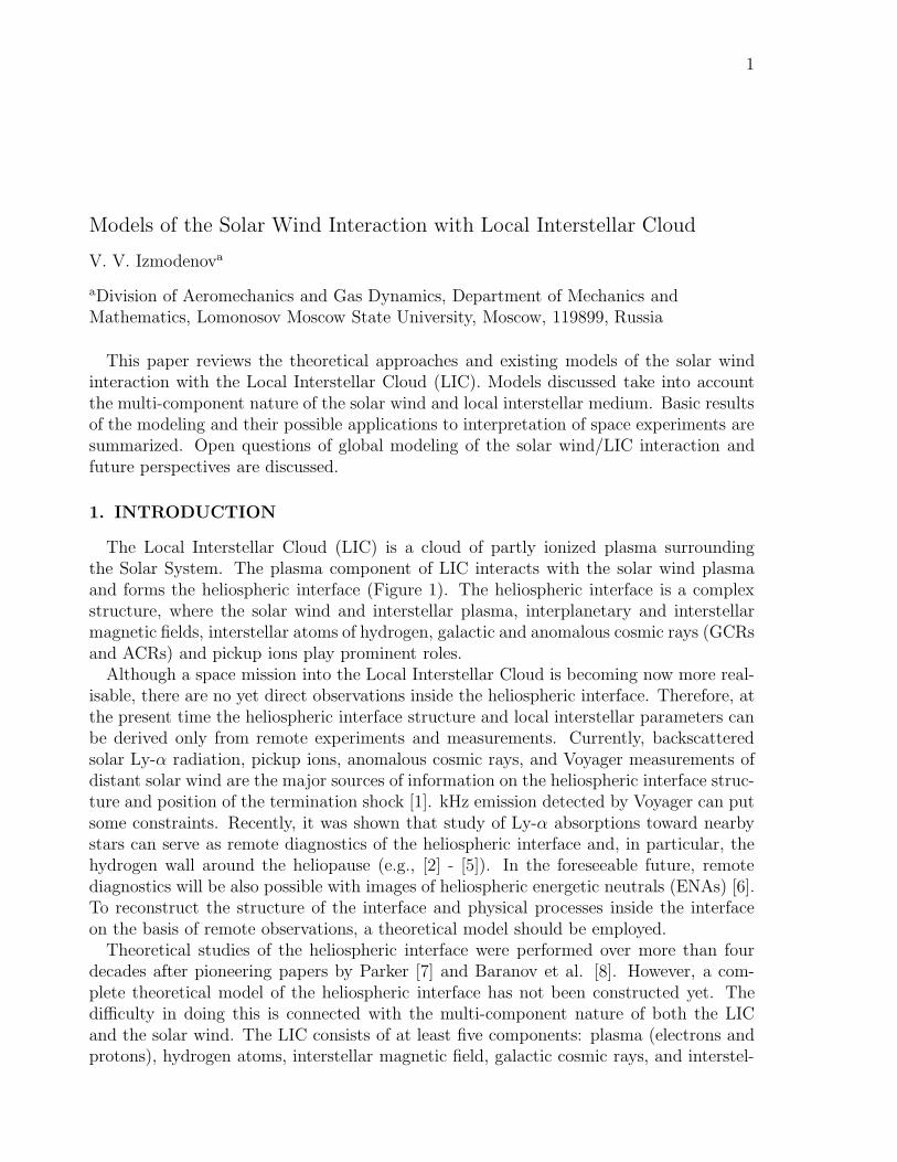
The Local Interstellar Cloud (LIC) is a cloud of partly ionized plasma surroundingthe Solar System. The plasma component of LIC interacts with the solar wind plasmaand forms the heliospheric interface (Figure 1). The heliospheric interface is a complexstructure, where the solar wind and interstellar plasma, interplanetary and interstellarmagnetic fields, interstellar atoms of hydrogen, galactic and anomalous cosmic rays (GCRsand ACRs) and pickup ions play prominent roles.

Although a space mission into the Local Interstellar Cloud is becoming now more real-isable, there are no yet direct observations inside the heliospheric interface. Therefore, atthe present time the heliospheric interface structure and local interstellar parameters canbe derived only from remote experiments and measurements. Currently, backscatteredsolar Ly-α radiation, pickup ions, anomalous cosmic rays, and Voyager measurements ofdistant solar wind are the major sources of information on the heliospheric interface struc-ture and position of the termination shock [1]. kHz emission detected by Voyager can putsome constraints. Recently, it was shown that study of Ly-α absorptions toward nearbystars can serve as remote diagnostics of the heliospheric interface and, in particular, thehydrogen wall around the heliopause (e.g., [2] - [5]). In the foreseeable future, remotediagnostics will be also possible with images of heliospheric energetic neutrals (ENAs) [6].To reconstruct the structure of the interface and physical processes inside the interfaceon the basis of remote observations, a theoretical model should be employed.

Theoretical studies of the heliospheric interface were performed over more than fourdecades after pioneering papers by Parker [7] and Baranov et al. [8]. However, a com-plete theoretical model of the heliospheric interface has not been constructed yet. Thedifficulty in doing this is connected with the multi-component nature of both the LICand the solar wind. The LIC consists of at least five components: plasma (electrons andprotons), hydrogen atoms, interstellar magnetic field, galactic cosmic rays, and interstel-

2

e, pH

LISM

SW

Termination

shock

Bow

shoc

k

Heliopause

Region 4Region 3

Region 2

Region 1

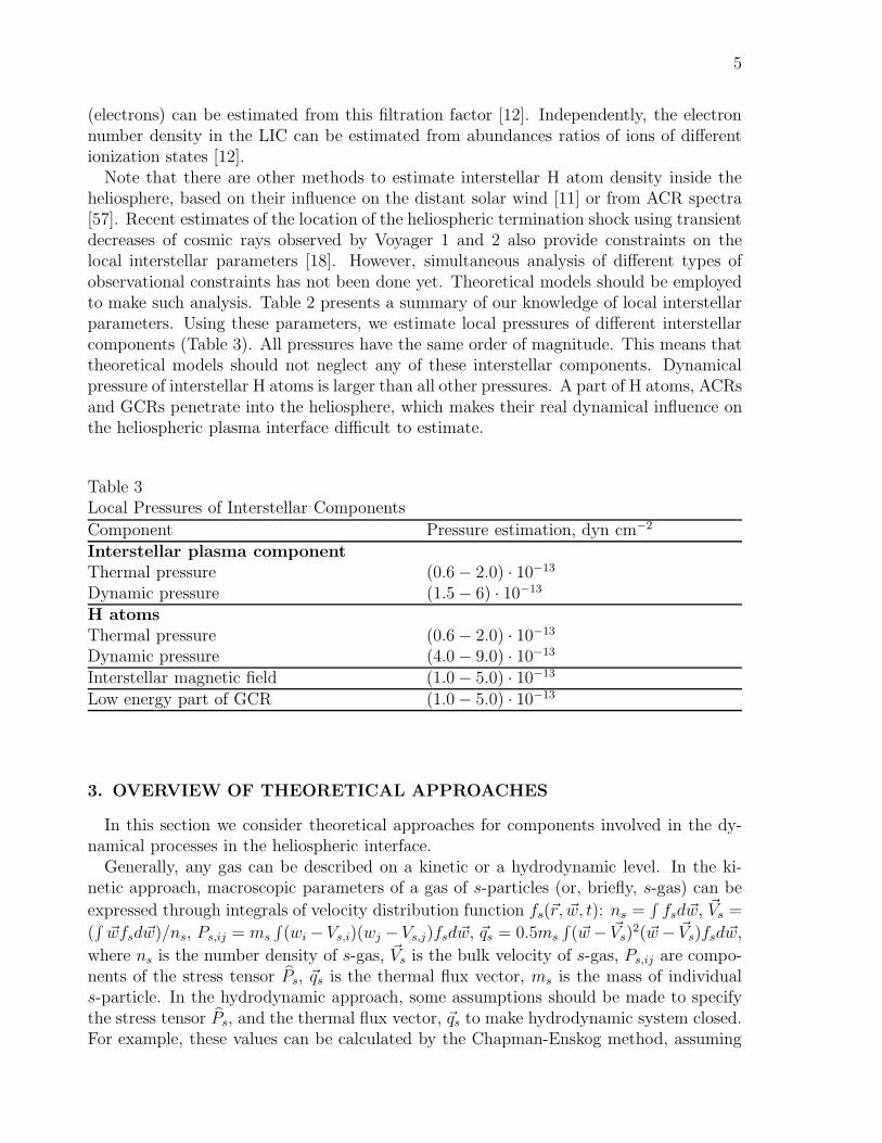
Figure 1. The heliospheric interface is the region of the solar wind interaction withLIC. The heliopause is a contact discontinuity, which separates the plasma wind frominterstellar plasmas. The termination shock decelerates the supersonic solar wind. Thebow shock may also exist in the interstellar medium. The heliospheric interface can bedivided into four regions with significantly different plasma properties: 1) supersonic solarwind; 2) subsonic solar wind in the region between the heliopause and termination shock;3) disturbed interstellar plasma region (or ”pile-up” region) around the heliopause; 4)undisturbed interstellar medium.

lar dust. The heliospheric plasma consists of original solar particles (protons, electrons,alpha particles, etc.), pickup ions and the anomalous cosmic ray component. The pickupion component is a result of ionization of those interstellar H atoms that penetrate intothe heliosphere through the heliospheric interface. A part of the pickup ions is acceleratedto high energies of ACRs. ACRs may also modify the plasma flow upstream of the ter-mination shock and in the heliosheath. Spectra of ACRs can serve as remote diagnosticsof the termination shock. For a recent review on ACRs see [9].

To construct a theoretical model of the heliospheric interface, one needs to choose a spe-cific approach for each interstellar and solar wind component. Interstellar and solar windprotons and electrons can probably be described as fluids. At the same time interstellarH atom flow requires kinetic description. For pickup ion and cosmic ray components,the kinetic approach is also required. However, for interpretations that are not directlyconnected to pickup ions and ACRs, a cruder model can be used.

3

Table 1Number Densities and Pressures of Solar Wind Components

Component 4-5 AU 80 AUNumber Density Pressure Number Density Pressure

cm−3 eV/cm−3 cm−3 eV/cm−3

Original solar 0.2-0.4 2.-4. (thermal) (7− 14) · 10−4 10−3 - 10−4

wind protons ∼ 200 (dynamic) ∼ 0.5− 1. (dynamic)Pickup ions 5.1 · 10−4 0.5 ∼ 2 · 10−4 ∼ 0.15Anomalouscosmic rays 0.01 - 0.1

This paper focuses on the models of the global heliospheric interface structure. Underglobal models I understand those models that study the whole interaction region, includingthe termination shock, the heliopause and possible bow shock. In this sense, this papershould not be considered as a complete review of progress in the field. Many differentapproaches were used to look into different aspects of the solar wind interaction withLIC connecting with pickup ion transport and acceleration, with the termination shockstructure under influence of ACRs and pickup ions. For more complete overview see recentreviews [10],[9].

The structure of the paper is the following: The next section briefly describes ourcurrent knowledge of the local interstellar and solar wind parameters. Section 3 discussestheoretical approaches to be used for the interstellar and solar wind components. Section4 gives an overview of heliospheric interface models. Section 5 describes basic resultsof the Baranov-Malama model of the heliospheric interface and its future developments.In section 6 we demonstrate possible analyses of space experiments on the basis of atheoretical model of the heliospheric interface. Section 7 underlines current problems inthe modeling of the global heliosphere and discusses future perspectives.

2. BRIEF SUMMARY OF OBSERVATIONAL KNOWLEDGE

Choice of an adequate theoretical model of the heliospheric interface depends on bound-ary conditions, i.e. on undisturbed solar wind and interstellar parameters.

2.1. Solar wind observationsAt the Earth’s orbit the flux of interstellar atoms is quite small, and the solar wind

can be considered undisturbed. Measurements of pickup ions and ACRs also show thatthese components do not have dynamical influences on the original solar wind particlesat the Earth’s orbit. Therefore, solar wind parameters at the Earth’s orbit can be takenas inner boundary conditions.

It has been shown by many authors that pickup and ACR components dynamicallyinfluence the solar wind at large heliocentric distances. Observable evidence of suchinfluence is, for example, deceleration of the solar wind detected by Voyager [11]. Table 1presents estimates of dynamic importance of the heliospheric plasma components at smalland large heliocentric distances. The table shows that pickup ion thermal pressure canbe up to 30-50 % of the dynamic pressure of solar wind.

4

Table 2Local Interstellar ParametersParameter Direct measurements/estimationsSun/LIC relative velocity 25.3 ± 0.4 km s−1 (direct He atoms 1)

25.7 km s−1 (Doppler-shiftedabsorption lines 2)

Local interstellar temperature 7000 ± 600 K (direct He atoms 1)6700 K (absorption lines 2)

LIC H atoms number density 0.2 ± 0.05 cm−3 (estimate based onpickup ion observations 3)

LIC proton number density 0.03 - 0.1 cm−3 (estimate based onpickup ion observations 3)

Local Interstellar magnetic field Magnitude: 2-4 µGDirection: unknown

Pressure of low energetic part of cosmic rays ∼0.2 eV cm−3

1[13]; 2 [12]; 3 [19]

2.2. Interstellar parametersLocal interstellar temperature and velocity can be inferred from direct measurements of

interstellar atoms of helium by Ulysses/GAS instrument [13]. Atoms of interstellar heliumpenetrate the heliospheric interface undisturbed, because of the small strength of theircoupling with interstellar and solar wind protons. Indeed, due to small cross sections ofelastic collisions and charge exchange with protons, the mean free path of these atoms islarger than the heliospheric interface. Independently, the velocity and temperature in theLocal Interstellar Cloud can be deduced from analysis of absorption features in the stellarspectra [12]. However, this method provides mean values along the line of sight in theLIC. A comparison of local interstellar temperatures and velocities derived from stellarabsorption with those derived from direct measurements of interstellar helium shows quitegood agreement (see Table 2).

Other local parameters of the interstellar medium, such as interstellar H atom and elec-tron number densities, and strength and direction of the interstellar magnetic field, are notwell known. In the models they can be considered as free parameters. However, measure-ments of interstellar H atoms and their derivatives as pickup ions and ACRs provide im-portant constraints on local interstellar densities and total pressure. The neutral H densityin the inner heliosphere depends on filtration the neutral H atoms in the heliospheric inter-face due to charge exchange. Since interstellar He is not perturbed in the interface, localinterstellar number density of H atoms can be estimated from the neutral hydrogen to theneutral helium ratio in the LIC, R(HI/HeI)LIC: nLIC(HI) = R(HI/HeI)LICnLIC(HeI).The neutral He number density in the heliosphere has been recently determined to be verylikely around 0.013 − 0.018 cm−3 ([13] - [15]). Interstellar ratio HI/HeI is likely in therange of 10-14. Therefore, expected interstellar H atom number densities are in the rangeof 0.13− 0.25 cm−3. It was shown by modeling [16], [17] that the filtration factor, whichis the ratio of neutral H density inside and outside the heliosphere, is a function of in-terstellar plasma number density. Therefore, the number density of interstellar protons

5

(electrons) can be estimated from this filtration factor [12]. Independently, the electronnumber density in the LIC can be estimated from abundances ratios of ions of differentionization states [12].

Note that there are other methods to estimate interstellar H atom density inside theheliosphere, based on their influence on the distant solar wind [11] or from ACR spectra[57]. Recent estimates of the location of the heliospheric termination shock using transientdecreases of cosmic rays observed by Voyager 1 and 2 also provide constraints on thelocal interstellar parameters [18]. However, simultaneous analysis of different types ofobservational constraints has not been done yet. Theoretical models should be employedto make such analysis. Table 2 presents a summary of our knowledge of local interstellarparameters. Using these parameters, we estimate local pressures of different interstellarcomponents (Table 3). All pressures have the same order of magnitude. This means thattheoretical models should not neglect any of these interstellar components. Dynamicalpressure of interstellar H atoms is larger than all other pressures. A part of H atoms, ACRsand GCRs penetrate into the heliosphere, which makes their real dynamical influence onthe heliospheric plasma interface difficult to estimate.

Table 3Local Pressures of Interstellar Components

Component Pressure estimation, dyn cm−2

Interstellar plasma componentThermal pressure (0.6− 2.0) · 10−13

Dynamic pressure (1.5− 6) · 10−13

H atomsThermal pressure (0.6− 2.0) · 10−13

Dynamic pressure (4.0− 9.0) · 10−13

Interstellar magnetic field (1.0− 5.0) · 10−13

Low energy part of GCR (1.0− 5.0) · 10−13

3. OVERVIEW OF THEORETICAL APPROACHES

In this section we consider theoretical approaches for components involved in the dy-namical processes in the heliospheric interface.

Generally, any gas can be described on a kinetic or a hydrodynamic level. In the ki-netic approach, macroscopic parameters of a gas of s-particles (or, briefly, s-gas) can be

expressed through integrals of velocity distribution function fs(~r, ~w, t): ns =∫

fsd~w, ~Vs =

(∫

~wfsd~w)/ns, Ps,ij = ms

∫(wi− Vs,i)(wj − Vs,j)fsd~w, ~qs = 0.5ms

∫(~w− ~Vs)

2(~w− ~Vs)fsd~w,

where ns is the number density of s-gas, ~Vs is the bulk velocity of s-gas, Ps,ij are compo-nents of the stress tensor P̂s, ~qs is the thermal flux vector, ms is the mass of individuals-particle. In the hydrodynamic approach, some assumptions should be made to specifythe stress tensor P̂s, and the thermal flux vector, ~qs to make hydrodynamic system closed.For example, these values can be calculated by the Chapman-Enskog method, assuming

6

Kn = l/L << 1, where l and L are the mean free path of the particles and character-istic size of the problem, respectively. The zero approximation of the Chapman-Enskogmethod gives local Maxwellian distribution, and the gas can be considered as an idealgas, where the stress tensor reduces to scalar pressure P and ~q = 0.

3.1. H atomsInterstellar atoms of hydrogen form the most abundant component in the circumsolar

local interstellar medium (see, Table 2). These atoms penetrate deep into the heliosphereand interact with interstellar and solar wind plasma protons. The cross sections of elasticH-H, H-p collisions are negligible as compared with the charge exchange cross section[20]. Charge exchange with solar wind/interstellar protons determines the properties ofthe H atom gas in the interface. Atoms, newly created by charge exchange, have thelocal properties of protons. Since plasma properties are different in the four regionsof the heliospheric interface shown in Figure 1, the H atoms can be separated into fourpopulations, each having significantly different properties. The strength of H atom-protoncoupling can be estimated through the calculation of mean free path of H atoms in plasma.Generally, the mean free path (with respect to the momentum transfer) of s-particle int-gas can be calculated by the formula: l = msw

2s/(δMst/δt). Here, ws is the individual

velocity of s-particle, and δMst/δt is individual s-particle momentum transfer rate in t-gas.Table 4 shows the mean free paths of H atoms with respect to charge exchange with

protons. The mean free paths are calculated for typical atoms of different populations atdifferent regions of the interface in the upwind direction. For every population of H atoms,there is at least one region in the interface where the Knudsen number Kn ≈ 0.5 − 1.0.Therefore, the kinetic Boltzmann approach must be used to describe interstellar atoms inthe heliospheric interface.

Table 4Mean free paths of H-atoms in the heliospheric interface with respect to charge exchangewith protons, in AU.

Population At TS At HP Between HP and BS LISM4 (primary interstellar) 150 100 110 8703 (secondary interstellar) 66 40 58 1902 (atoms originating in the heliosheath) 830 200 110 2001 (neutralized solar wind) 16000 510 240 490

The velocity distribution of H atoms fH(~r, ~wH, t) may be calculated from the linearkinetic equation introduced in [51]:

∂fH

∂t+ ~wH · ∂fH

∂~r+

~F

mH

· ∂fH

∂ ~wH

= −fH

∫|~wH − ~wp|σHP

ex fp(~r, ~wp)d~wp (1)

+fp(~r, ~wH)∫|~w∗H − ~wH|σHP

ex fH(~r, ~w∗H)d~w∗H − (νph + νimpact)fH(~r, ~wH).

Here fH(~r, ~wH) is the distribution function of H atoms; fp(~r, ~wp) is the local distributionfunction of protons; ~wp and ~wH are the individual proton and H atom velocities, respec-

7

tively; σHPex is the charge exchange cross section of an H atom with a proton; νph is the

photoionization rate; mH is the atomic mass; νimpact is the electron impact ionization

rate; and ~F is the sum of the solar gravitational force and the solar radiation pressureforce. The plasma and neutral components interact mainly by charge exchange. However,photoionization, solar gravitation, and radiation pressure, which are taken into accountin equation (1), are important at small heliocentric distances. Electron impact ionizationmay be important in the heliosheath (region 2). The interaction of the plasma and Hatom components leads to the mutual exchanges of mass, momentum and energy. Theseexchanges should be taken into account in the plasma equations through source terms,which are integrals of fH(~r, ~w, t).

3.2. Solar wind and interstellar electron and proton componentsBasic assumptions necessary to employ a hydrodynamic approach for space plasmas

were reviewed in [21]. In particular, it was concluded in the paper that interstellar andsolar wind plasmas can be treated hydrodynamically. Indeed, the mean free path of thecharged particles in the local interstellar plasma is less than 1 AU, which is much smallerthan the size of the heliospheric interface itself. Therefore, the local interstellar plasma iscollisional plasma, and a hydrodynamic approach can be used to describe it. Solar windplasma is collisionless, because the mean free path of the solar wind particles is muchlarger than the size of the heliopause. Therefore, the heliospheric termination shock (TS)is a collisionless shock. A hydrodynamic approach can be justified for collisionless plasmaswhen scattering of charged particles on plasma fluctuations is efficient (”collective plasmaprocesses”). In this case, the mean free path l with respect to collisions is replaced by lcoll,the mean free path of collective processes, which is assumed to be less than the character-istic length of the problem L: lcoll << L. However, the integral of ”collective collisions” istoo complicated to be used to calculate the transport coefficient for collisionless plasmas.

One-fluid description of heliospheric and interstellar plasmas is commonly used in theglobal models of the heliospheric interface. However, since measurements of the solar windshow different electron and proton temperatures, two-fluid approach is more appropriate.The temperatures may remain different up to the termination shock and beyond due tothe weak energy exchange between protons and electrons.

Hydrodynamic Euler equations for proton and electron components, which take intoaccount the influence of other components such as interstellar H atoms, pickup ions,cosmic rays, electric and magnetic fields, are written below. Mass balance or continuityequations are

∂ns

∂t+∇ · (ns

~Vs) = q1,s, (s = e, p) (2)

Index e denotes electrons, index p denotes solar wind protons. q1,e = nH ·(νph +νimpact),q1,p = − ∫ uσHP

ex (u)fp(~w)fH(~wH)d~wd~wH are sources and sinks due to charge exchange, pho-toionization and electron impact ionization. Here, u = |~wH−~w| is the relative atom-protonvelocity, and ~wH and ~w are individual velocities of H atoms and protons, respectively. Mo-mentum balance equations are

∂(nsms~Vs)

∂t+∇Ps + ms∇ · (ns

~Vs ⊗ ~Vs)− nses( ~E +1

c[~Vs × ~B]) +

∑r

~Rsr = ms~q2,s (3)

8

where ~q2,e =∫(νph+νimpact)~wHfH(~wH)d~wH , ~q2,p = − ∫ ∫ uσHP

ex (u)~wpfH(~wH)fp(~wp)d~wHd~wp

and ~Rsr is the rate of momentum transfer from the r-gas component to the s-gas com-ponent. The symbol ⊗ represents the dyadic product. The momentum transfer term ~Rsr

can be expressed in a general form through the collision integral Ssr of kinetic equationof the s-gas component: ~Rsr = − ∫ ms~csSsrdcs, where ~cs = ~ws − ~Vs. That ~Rsr + ~Rrs = 0is a consequence of this definition of ~Rsr.

Heat balance equations have the following form:

∂

∂t

(3

2Ps

)+∇

(3

2Ps

~Vs

)+ Ps∇ · ~Vs =

∑r

Qsr + msq3,s −ms~q2,s · ~Vs (4)

with q3,e =∫

(νph + νimpact)~w2

H

2fH(~wH)d~wH ,

q3,p = − ∫ ∫ uσHPex (u)

~w2p

2fH(~wH)fp(~wp)d~wpd~vH . Qsr is the heat source due to interactions

between between particles of s and r components. Those terms can be expressed in a

general form through the collision term Ssr of the kinetic equation Qsr = − ∫ msc2s2

Sprdcs.As a result of this interaction, we have a relation connecting Qsr and Qrs: Qsr + Qrs =−~Rsr · (~Vs − ~Vr)(∀s 6= r).

System (2)-(4) should be added by the state equations: Pα = nαkTα (α = e, p), wherek is Boltzman constant, and Maxwell equations:

∇× ~E = −1

c

∂ ~B

∂t;∇ · ~E = 4πρe;∇× ~B =

4π

c~j;∇ · ~B = 0 (5)

where ρe is the charge density, e is the charge of electron, and ~j is current density.The displacement current has been dropped. Note, that charge and current densitiesof all charged populations should be taken into account in (5). Neglecting cosmic ray

charges and currents we have ρe = e(np + npui − ne) and ~j = e(np~Vp − ne

~Ve + npui~Vpui).

The number density of pickup ions, npui, and the bulk velocity of pickup ions, ~Vpui are

integrals of pickup proton velocity distribution function: npui =∫

fpui(~w)d~w, ~Vpui =(∫

~wfpui(~w)d~w)/npui.Note that in equations (2)-(4) we assume that pickup electrons are indistinguishable

from original solar wind electrons, while pickup protons are considered as a separatepopulation.

The expressions for various interaction terms ~Rsr, Qs (s = e, p)must be specified.Electron-proton collision terms can be taken in the form given by Braginski [22]:

~Rep = −mene

τe~ue (6)

Qpe = Qep − Rep~ue =3ne

τe

me

mp

k(Te − Tp) (7)

Here, ne is the electron number density; Te and Tp are electron and proton densities,respectively; me and mp are the electron and proton masses; ~ue is the electron velocityrelative to the proton rest frame. Parameter τe characterizes the coupling between elec-trons and protons and corresponds to the electron collision time for collisional plasma[22]. In collisionless heliospheric plasma, additional assumptions are needed to determineτe; otherwise, it can be considered as free parameter.

9

3.3. Pickup ionsTo study pickup ion dynamical influence on the distant solar wind, the termination

shock structure and, finally, on the global heliospheric interface structure, details of theprocess of charged particle assimilation into the magnetized plasma are needed. A newlycreated ion under the influence of the steady solar wind electric and magnetic fieldsexecutes a cycloidal trajectory with the guiding center, which is drifting at the bulkvelocity of the solar wind. Assuming that the gyroradius is much smaller than the typicalscale length, one can average velocity distribution function over the gyratory motion.Initial ring-beam distribution of pickup ions is unstable. Basic processes that determineevolution of pickup ion distribution are pitch-angle scattering, energy diffusion in thewave field generated by both pickup ions and the solar wind waves, convection, adiabaticcooling in the expanding solar wind, and injection of newly ionized particles. The mostgeneral form of the relevant transport equation to describe the evolution of gyrotropicvelocity distribution function fpui = fpui(t, ~r, v, µ) of pickup ions in a background plasma

moving at a velocity ~Vsw were written in [23], [24]. fpui is a function of the modulus ofvelocity in the solar wind rest frame, and µ is the cosine of pitch angle.

Complete assimilation of pickup ions into the solar wind would result in a great in-crease in the temperature with increasing heliocentric distance, which is not observed.Therefore, the solar wind and pickup protons represent two distinct proton populations.Nevertheless, the radial temperature profile of protons measured by Voyager 2 shows asmaller decrease as compared with the adiabatic cooling. A fraction of heating of so-lar wind protons may be connected with pickup generated waves [25]. Many aspects ofpickup ion evolution were studied ( e.g., [24]; for review, see [10], [9]). However, today itstill seems to be impossible to take into account all details of the assimilation process ofpickup ions into the solar wind in the global models of the heliospheric interface structure.Instead, one may try to use the hydrodynamic approach. In this approach, equations (2)-(4) written for pickup ions represent the balance of their mass, momentum and energy.The right sides of the equations include sources of pickup ions due to ionization processes:

q1,pui = nHνph +∫

uσHPex (u)fH(~wH)fp(~w)d~wd~vH

~q2,pui =∫

(νph + νimpact)~vHfH(~vH)d~vH +∫ ∫

uσHPex (u)~wHfH(~wH)fp(~wp)d~wHd~wp+

∫ ∫uσHP

ex (u)(~wH − ~wi)fH(~wH)fpui(~wi)d~wHd~wi

q3,pui =∫

(νph + νimpact)~w2

H

2fH(~wH)fp(~wp)d~wpd~wH

+∫ ∫

uσHPex (u)

~w2H − ~w2

i

2fH(~wH)fpui(~wi)d~wid~wH

To complete the model, one should also specify interaction terms ~Rpui,r, Qpui,r (r 6= pui).The specification of these terms for pickup ion-proton interactions requires analysis of thepickup process in detail at the kinetic level. Global models usually assume immediateassimilation of pickup ions into the solar wind (one-fluid model) or perfect co-moving of

10

these populations Vp = Vpui and no exchange of energy Qpui,p = 0 (two- or three-fluidmodels). Energy exchange term of pickup with ACRs, Qpui,acr = −Qacr,pui, is specified innext subsection.

3.4. Cosmic raysThe cosmic rays are coupled to background flow via scattering with plasma waves. The

net effect is that the cosmic rays tend to be convected along with the background plasmaas they diffuse through the magnetic irregularities carried by the background plasma.Both galactic and anomalous cosmic rays can be treated as populations with negligiblemass density and sufficient energy density. At a hydrodynamical level, the cosmic raysmay modify the wind flow via their pressure gradient ∇Pc with the net energy transferrate from fluid to the cosmic rays given by ~V · ∇Pc. Pc(~r, t) = 4π

3

∫∞0 fc(~r, p, t)wp3dp is a

cosmic ray pressure; fc(~r, p, t) is the isotropic velocity distribution of cosmic rays.The transport equation of these particles has the following form [9]:

∂fc

∂t=

1

p2

∂

∂p

(p2D

∂fc

∂p

)+∇(k̂∇fc)− ~V · ∇fc +

1

3(∇ · ~V )

∂fc

∂lnp+ S(~r, p, t) (8)

Here p is the modulus of the momentum of the particle; D is the diffusion coefficientin momentum space, often assumed to be zero; k̂ is the tensor of spatial diffusion; ~V =~U + ~Vdrift is the convection velocity; ~U is the plasma bulk velocity; ~Vdrift is a drift velocityin the heliospheric or interstellar magnetic field; and S(~r, p, t) is the source term.

At the hydrodynamic level, the transport equation of the cosmic rays in the heliosphericinterface is:

∂Pc

∂t= ∇[k̂∇Pc − γc(~U + Udr)Pc] + (γc − 1)~U · ∇Pc + Qacr,pui(~r, t) (9)

Here we assume that D = 0; Udr is momentum-averaged drift velocity; γ is the polytropicindex; and Qacr,pui is the energy injection rate describing energy gains of the ACRs from

pickup ions. Chalov and Fahr ([26], [27]) suggested that Qacr,pui = −αppuidiv~U , where αis a constant injection efficiency defined by the specific plasma properties [27]. α is set tozero for GCRs since no injection occurs into the GCR component.

4. OVERVIEW OF HELIOSPHERIC INTERFACE MODELS

Together with Maxwellian equations (5) the Boltzman equation (1) for interstellar Hatoms; sets of hydrodynamic equations (2)-(4) written for solar protons, electrons andpickup ions; and equation (9) written for anomalous and cosmic ray components form

a closed system of equations, when interaction terms ~Rsr, Qsr are specified. Possiblespecification of the interaction terms is given in equations (6), (7). We have to note here,that such a complete model has yet to be developed. However, in recent years, severalgroups have focused their efforts on theory and modeling in order to understand someeffects separately from others. In particular, the influence of the interstellar magnetic fieldon the interface structure was studied in [28]- [31] for the two-dimensional case and in[32] and [33] for the three-dimensional case. Both interstellar and interplanetary magneticfields were considered in [34] and [35]. A comparison of these MHD models was givenrecently in [36]. Latitudinal variations of the solar wind have been considered in [37]. The

11

influence of the solar cycle variations on the heliospheric interface was studied in the 2Dcase in [38] - [42] and in [35] for the 3D case. In spite of many interesting findings in thepapers cited above, these theoretical studies did not take into account the interstellar Hatoms, or took them into account but under greatly simplified assumptions, as it was donein [34], where velocity and temperature of interstellar H atoms were assumed as constantsin the entire interface.

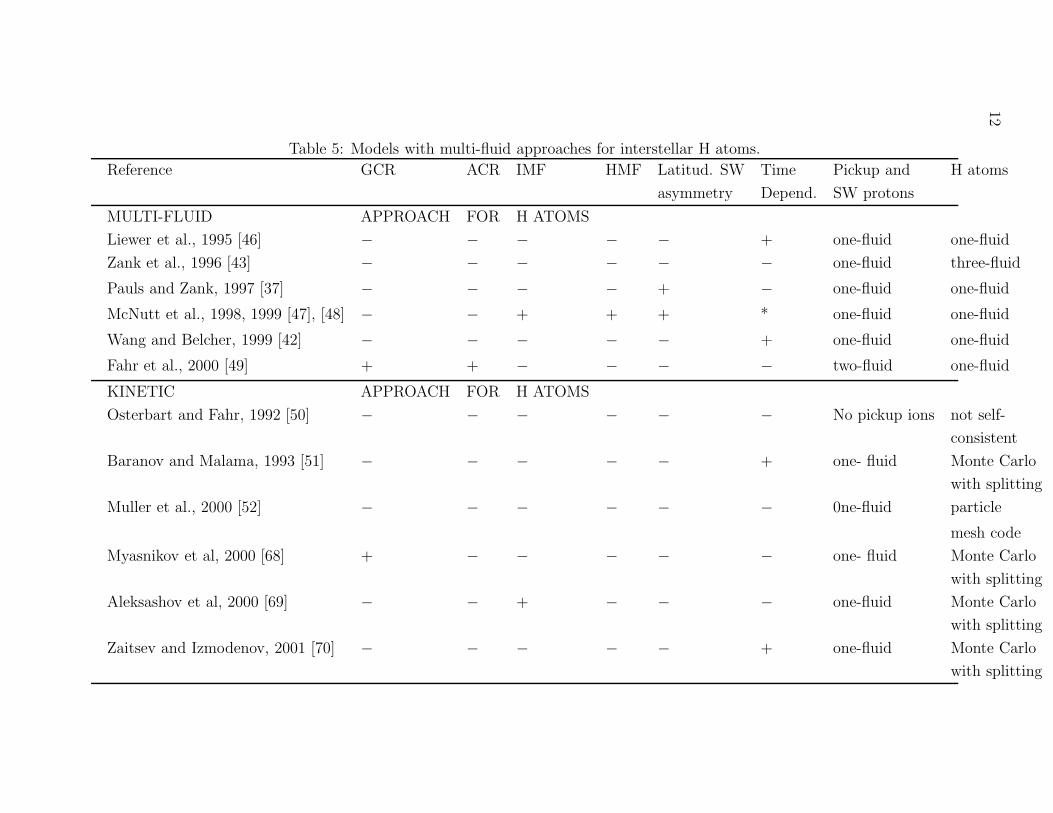
Since most of the observational information on the heliospheric interface is connectedwith interstellar neutrals and their derivatives as pickup ions and ACRs, we will focus onthe models, which include interstellar neutrals in a more appropriate way. These modelscan be separated into two types. Models of the first type (Table 5) use a simplified fluid(or multi-fluid) approach for interstellar H atoms. A kinetic approach was used in themodels of the second type. Development of the fluid (or multi-fluid) models of H atomswas connected with the fact that fluid (or multi-fluid) approach is simpler for numericalrealization. At the same time such an approach can lead to nonphysical results. Resultsof one of the most sophisticated multi-fluid models [43] were compared with the kineticBaranov-Malama model in [44]. The comparison shows qualitative and quantitative dis-agreements in distributions of H atoms. At the same time, it was concluded in [45] thatthe two models agreed on the distances to the termination shock, heliopause and bowshock in upwind, but not in positions of the termination shock in downwind.

4.1. One-fluid plasma modelsOne of the common features in the models [42], [43], [46] - [48], [51], [52], [67]-[69]

is that proton, electron and pickup ion components were considered as one fluid. Thegreat advantage of this approach is that its equations are considerably simpler than thethree- and two-fluid approaches (see next subsection). A key assumption of this approachis immediate assimilation of pickup protons into the original solar protons. In otherwords, it is assumed that immediately after ionization one cannot distinguish betweenoriginal solar protons and pickup protons. Another important assumption is that electronand proton components have equal temperatures, Te = Tp. For quasineutral plasma(np + npui = ne + o(ne)) this means that the pressure of the electrons is equal to half oftotal pressure (P = nekTe + (np + npui)kTp ≈ 2nekTe = 2Pe). Let us denote total density

ρ = mene + mp(np + npui), bulk velocity ~V = (∑

s msns~Vs)/ρ (s = e, p, pui).

Governing equations for the one-fluid approach can be obtained by summarizing equa-tions (2)-(4) for indexes s = e, p, pui. Introducing solar wind protons and pickup ionsas co-moving and taking into account that me << mp yield one-fluid equations in theirgeneral form:

∂ρ

∂t+∇ · (ρ~V ) = q1, q1 = mpnH(νph + νimpact) (10)

∂(ρ~V )

∂t+∇P +∇ · (ρ~V ⊗ ~V )− ρe

~E − 1

c[~j × ~B] = ~q2 −∇ · neme~ue~ue (11)

Here ~j =∑

α nαeα~Vα, ρe =

∑α nαeα; ~q2 =

∑s ms~q2,s; ~us = ~Vs − ~V .

∂

∂t

(3

2P)

+∇ ·(

5

2P ~V

)− ~V · ∇P = −∇

(5

2Pe~ue

)+ q3 − ~q2 · ~V + (12)

12

Table 5: Models with multi-fluid approaches for interstellar H atoms.

Reference GCR ACR IMF HMF Latitud. SW Time Pickup and H atoms

asymmetry Depend. SW protons

MULTI-FLUID APPROACH FOR H ATOMS

Liewer et al., 1995 [46] − − − − − + one-fluid one-fluid

Zank et al., 1996 [43] − − − − − − one-fluid three-fluid

Pauls and Zank, 1997 [37] − − − − + − one-fluid one-fluid

McNutt et al., 1998, 1999 [47], [48] − − + + + * one-fluid one-fluid

Wang and Belcher, 1999 [42] − − − − − + one-fluid one-fluid

Fahr et al., 2000 [49] + + − − − − two-fluid one-fluid

KINETIC APPROACH FOR H ATOMS

Osterbart and Fahr, 1992 [50] − − − − − − No pickup ions not self-

consistent

Baranov and Malama, 1993 [51] − − − − − + one- fluid Monte Carlo

with splitting

Muller et al., 2000 [52] − − − − − − 0ne-fluid particle

mesh code

Myasnikov et al, 2000 [68] + − − − − − one- fluid Monte Carlo

with splitting

Aleksashov et al, 2000 [69] − − + − − − one-fluid Monte Carlo

with splitting

Zaitsev and Izmodenov, 2001 [70] − − − − − + one-fluid Monte Carlo

with splitting

13

(~j − ρe~V ) ·

(~E +

1

c~Ve × ~B +

me

ene

(~q2,p + ~q2,pui))

where q3 =∑

s msq3,s. The relative electron velocity is connected with vector ~j as follows:~j = ρe

~V − ene~ue. Note that to derive (12) we use a generalized form of Ohm’s law andneglect the terms proportional me/mp in it:

nee(

~E +1

c~Ve × ~B

)= −∇Pe + ~Rep + me(~q2,p + ~q2,pui − ~q2,e)

If we assume momentum transfer term ~Rep as in (6) and neglect the term ρe~V in quasineu-

tral plasma, Ohm’s law may be rewritten:

~E = −1

c[~V × ~B] +

me

τenee2~j +

1

ene

(1

c~j × ~B −∇Pe

)+

me

ene(~q2,p + ~q2,pui − ~q2,e) (13)

To derive the classical system of hydrodynamic equations applied for heliospheric in-terface in one-fluid models, one needs to ignore terms containing magnetic and electricfields in equations (11) and (12). If we also disregard the second-order term ∇neme~ue~ue

in (11) and ∇(5pe~ue/2) in (12), equations (10)-(12) together with kinetic equation (1) forH atoms form a closed system of equations.

To get from (10)-(13) a system of ideally conducting MHD equations with a magneticfield frozen in plasma, one obviously needs to make other assumptions in addition to thatof high conductivity, when Rm >> 1. Rm = 4πσV L/c2 is magnetic Reynolds number,with the electrical conductivity σ = nee

2τe/me, and V and L characteristic velocity and

length, respectively. Vanishing electron pressure gradients, the Hall term, ~j × ~B andlast term of (13) connected with the charge-exchange effect, corresponding terms in thegeneralized Ohm’s law (13) also must be ignored. Under these conditions, the Ohm’s law

has its classical form ~E = −1c[~V × ~B], and last term of heat flux equation (12) is equal

to j2/σ and can be neglected. Ideal MHD equations with source terms q1, ~q2, q3, on theright-hand sides were considered in [34], [47], [48], [69].

4.2. Three- and two-fluid plasma modelsFor solar wind, the one-fluid model assumes essentially that wave-particle interactions

are sufficient for pickup ions to assimilate quickly into the solar wind, becoming indistin-guishable from solar wind protons. However, as discussed above, Voyager observationshave shown that this is probably not the case. Pickup ions are unlikely to be assimi-lated completely. Instead, two co-moving thermal populations can be expected. A modelthat distinguishes the pickup ions from the solar wind ions was suggested by Isenbergin [71]. Electrons were considered as a third fluid. The key assumption in the model isthat pickup ions and solar wind protons are co-moving (Vp = Vpui). It was also assumedthat there is no exchange of thermal energy between solar wind protons and pickup ions.Isenberg’s approach consists of two continuity equations (2) for solar protons and pickupions; one momentum equation (11) and three energy equations (4) for solar wind protons,

electrons and pickup ions. In (11) Isenberg neglect term ρe~E, the last term and assumes

that ~j = c∇× ~B/(4π). In energy equations he disregards the energy exchange terms Qsr.Note that Isenberg used the simplified form of source terms suggested in [72] and appliedthese equations to the spherically symmetric solar wind upstream the termination shock.

14

Another two-fluid approach to model solar wind protons and pickup protons was de-veloped recently in [49]. This model also assumes that convection speed of pickup ionsis identical to that of solar wind protons. The pressure of pickup ions is calculated byassuming a rectangular shape of the pickup ion isotropic distribution function. In thiscase, the pressure can be expressed through pickup ion density ρi and solar wind bulkvelocity Vsw as

Ppui = ρpuiV2sw/5. (14)

Therefore, governing plasma equations are i) one-fluid equations for the mixture of solarprotons, pickup ions and electrons; ii) continuity equation for pickup ions; iii) two trans-port equations for ACRs and GCRs. The influence of cosmic ray components was takenas terms −∇(PACR + PGCR) and −~V · ∇(PACR + PGCR)− αPpuidiv(~V ) in the right-handside of the momentum and energy equations, respectively.

5. BARANOV-MALAMA MODEL OF THE HELIOSPHERIC INTERFACE

The first self-consistent model of the two-component (plasma and H atoms) LIC inter-action with the solar wind was developed by Baranov and Malama [51]. The interstellarwind is assumed to have uniform parallel flow in the model. The solar wind is assumed tobe spherically symmetric at the Earth’s orbit. Under these assumptions, the heliosphericinterface has axisymmetric structure.

Plasma and neutral components interact mainly by charge exchange. However, pho-toionization, solar gravity and solar radiation pressure, which are especially important inthe vicinity of the Sun, are also taken into account.

Kinetic and hydrodynamic approaches were used for the neutral and plasma compo-nents, respectively. The kinetic equation (1 for neutrals is solved together with the Eulerequations for one-fluid plasma (10) - (12). The influence of the interstellar neutrals istaken into account in the right-hand side of the Euler equations that contain source termsq1, ~q2, q3, which are integrals of the H atom distribution function fH(~VH) and can be cal-culated directly by the Monte Carlo method [56]. The set of kinetic and Euler equationsis solved by iterative procedure, as suggested in [55]. Supersonic boundary conditionswere used for the unperturbed interstellar plasma and for the solar wind plasma at theEarth’s orbit. The velocity distribution of interstellar atoms is assumed to be Maxwellianin the unperturbed LIC. The model results are discussed below in this section.

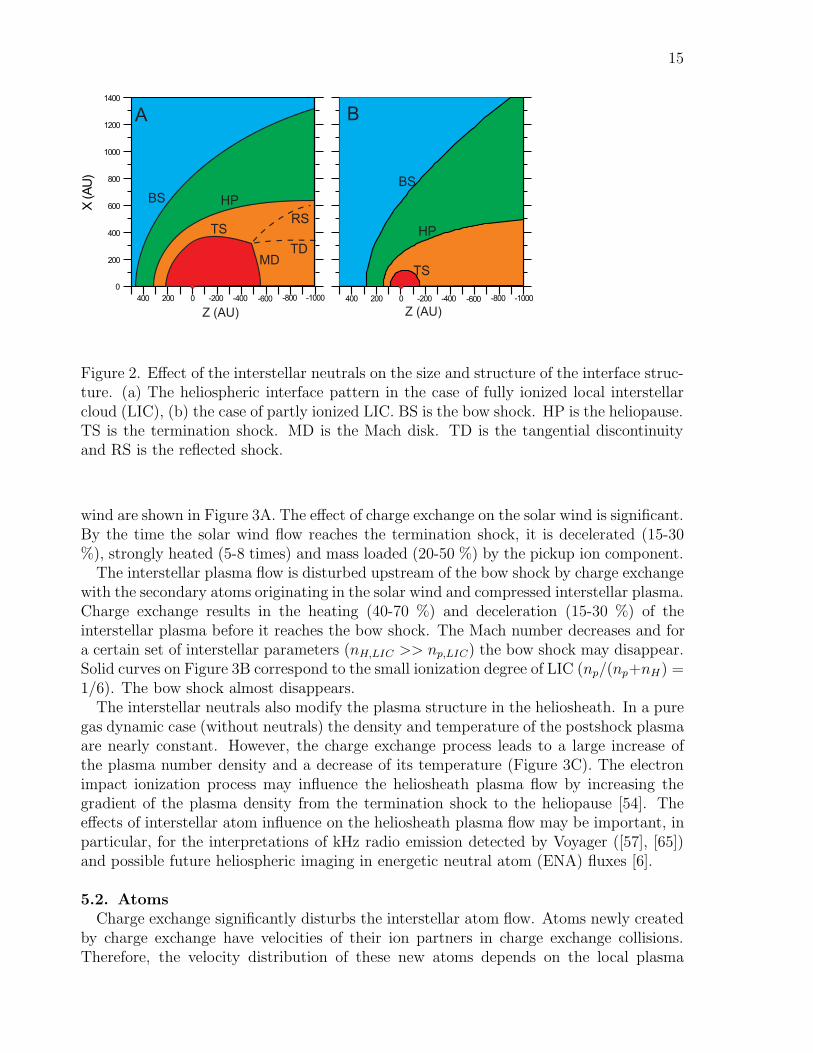
5.1. PlasmaInterstellar atoms strongly influence the heliospheric interface structure. In the presence

of interstellar neutrals, the heliospheric interface is much closer to the Sun than in a puregas dynamical case (Figure 2). The termination shock becomes more spherical. The Machdisk and the complicated shock structure in the tail disappear.

The supersonic plasma flows upstream of the bow and termination shocks are disturbed.The supersonic solar wind is disturbed by charge exchange with the interstellar neutrals.The new ions created by charge exchange are picked up by the solar wind magnetic field.The Baranov-Malama model assumes immediate assimilation of pickup ions into the solarwind plasma. The solar wind protons and pickup ions are treated as one-fluid, called thesolar wind. The number density, velocity, temperature, and Mach number of the solar

15

-1000-800-600-400-2000200400

BS HP

TS

MD

RS

TD

0

200

400

600

800

1000

1200

1400X

(AU

)

BS HP

TS

BS

HP

TS

-1000-800-600-400-2000200400

Z (AU)Z (AU)

A B

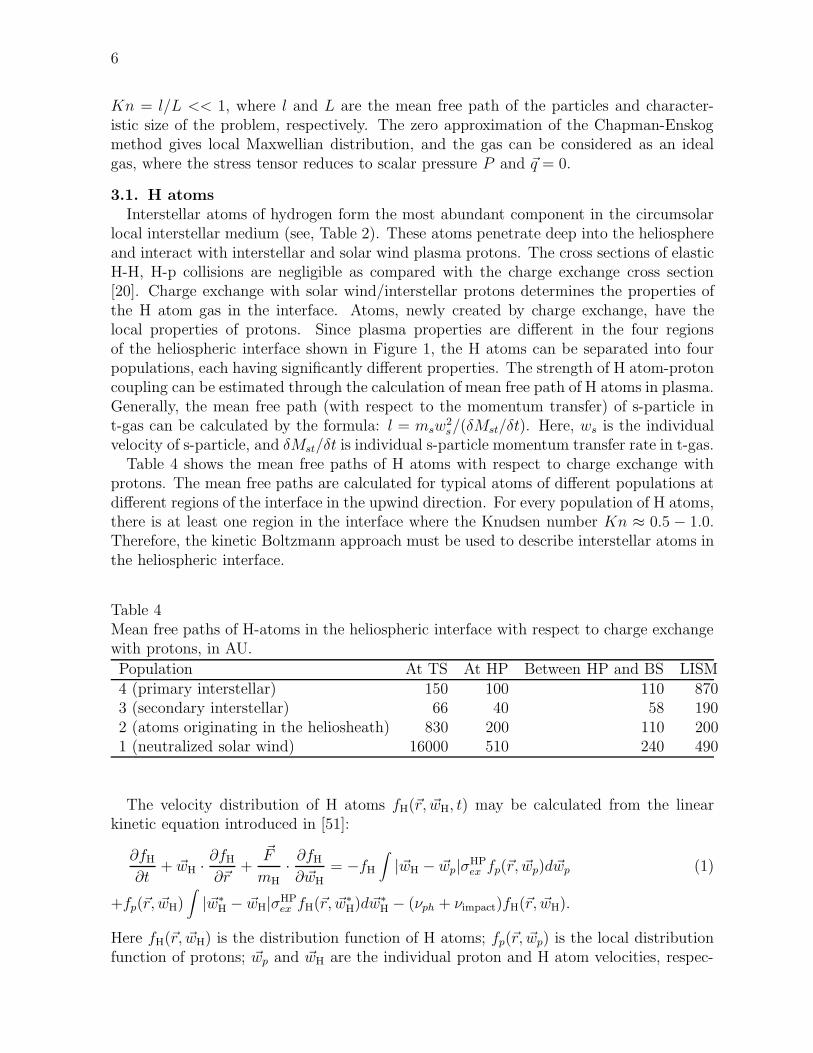
Figure 2. Effect of the interstellar neutrals on the size and structure of the interface struc-ture. (a) The heliospheric interface pattern in the case of fully ionized local interstellarcloud (LIC), (b) the case of partly ionized LIC. BS is the bow shock. HP is the heliopause.TS is the termination shock. MD is the Mach disk. TD is the tangential discontinuityand RS is the reflected shock.

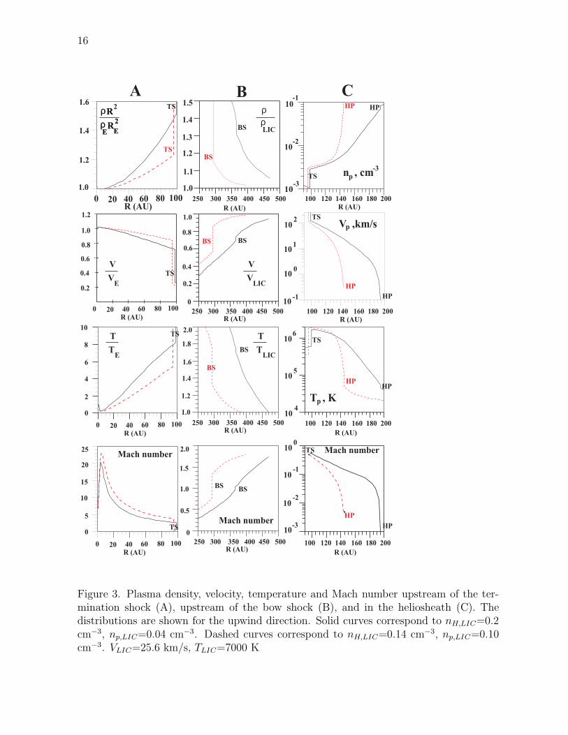
wind are shown in Figure 3A. The effect of charge exchange on the solar wind is significant.By the time the solar wind flow reaches the termination shock, it is decelerated (15-30%), strongly heated (5-8 times) and mass loaded (20-50 %) by the pickup ion component.

The interstellar plasma flow is disturbed upstream of the bow shock by charge exchangewith the secondary atoms originating in the solar wind and compressed interstellar plasma.Charge exchange results in the heating (40-70 %) and deceleration (15-30 %) of theinterstellar plasma before it reaches the bow shock. The Mach number decreases and fora certain set of interstellar parameters (nH,LIC >> np,LIC) the bow shock may disappear.Solid curves on Figure 3B correspond to the small ionization degree of LIC (np/(np+nH) =1/6). The bow shock almost disappears.

The interstellar neutrals also modify the plasma structure in the heliosheath. In a puregas dynamic case (without neutrals) the density and temperature of the postshock plasmaare nearly constant. However, the charge exchange process leads to a large increase ofthe plasma number density and a decrease of its temperature (Figure 3C). The electronimpact ionization process may influence the heliosheath plasma flow by increasing thegradient of the plasma density from the termination shock to the heliopause [54]. Theeffects of interstellar atom influence on the heliosheath plasma flow may be important, inparticular, for the interpretations of kHz radio emission detected by Voyager ([57], [65])and possible future heliospheric imaging in energetic neutral atom (ENA) fluxes [6].

5.2. AtomsCharge exchange significantly disturbs the interstellar atom flow. Atoms newly created

by charge exchange have velocities of their ion partners in charge exchange collisions.Therefore, the velocity distribution of these new atoms depends on the local plasma

16

1.0

1.2

1.4

1.6

Rρ 2

ρ R2

E E

0 20 40 60 80 100R (AU)

0 20 40 60 80 100

R (AU)

0

5

10

15

20

25Mach number

Mach number

250 300 350 400 450 500R (AU)

250 300 350 400 450 500

R (AU)

1.0

1.1

1.2

1.3

1.4

1.5TS

TS

BS

BS

ρρLIC

n , cm-3

pTS

HP HP

100 120 140 160 180 200

R (AU)

10

10

10

-1

-2

-3

1.2

1.0

0.8

0.6

0.4

0.2

10

8

6

4

2

0

0

0.5

1.0

1.5

2.0 Mach number

10

10

10

10

-3

-2

-1

0

10

10

10

10

10

10

10

2

1

0

-1

TS

HP

HP

HPHP

TS

4

5

6

V ,km/sp

T , Kp

A B C

BSBS

TS

TS

BS

BS

HP

HP

TS

BSBS

TS

Rρρ R

2

E E

V

VLIC

V

VE

1.0

0.8

0.6

0.4

0.2

0

T

TE

T

TLIC

2.0

1.0

1.2

1.4

1.6

1.8

100 120 140 160 180 200R (AU)

100 120 140 160 180 200R (AU)

250 300 350 400 450 500R (AU)

250 300 350 400 450 500R (AU)

100 120 140 160 180 200

R (AU)

0 20 40 60 80 100

R (AU)

0 20 40 60 80 100

R (AU)

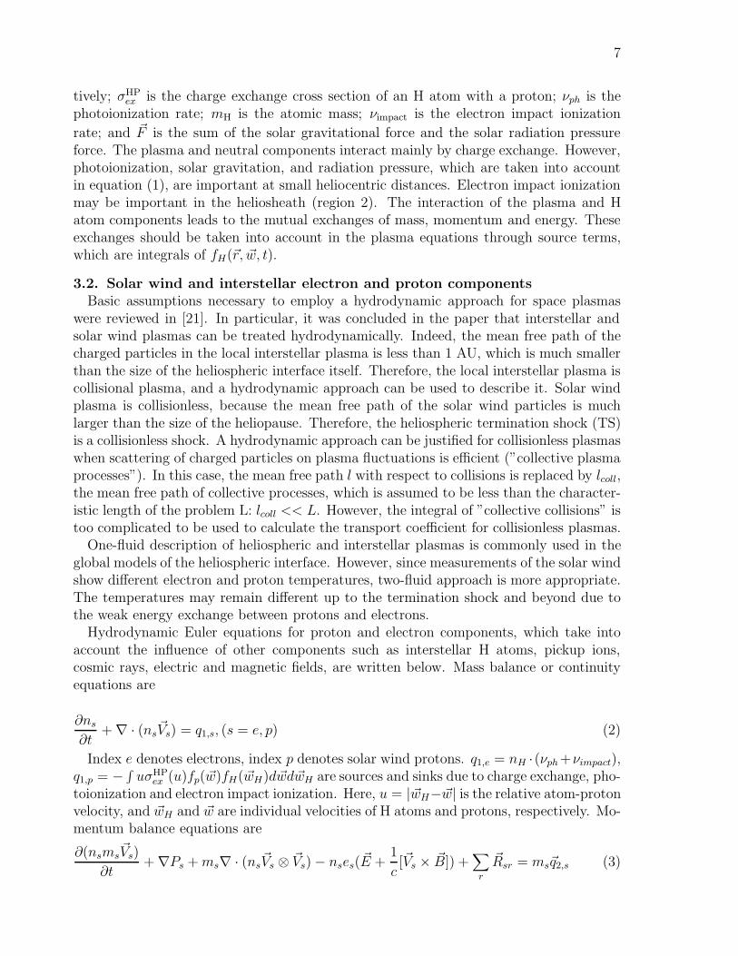
Figure 3. Plasma density, velocity, temperature and Mach number upstream of the ter-mination shock (A), upstream of the bow shock (B), and in the heliosheath (C). Thedistributions are shown for the upwind direction. Solid curves correspond to nH,LIC=0.2cm−3, np,LIC=0.04 cm−3. Dashed curves correspond to nH,LIC=0.14 cm−3, np,LIC=0.10cm−3. VLIC=25.6 km/s, TLIC=7000 K

17

0 100 200 300 400 500

0.0

0.5

1.0

0 100 200 300 400 500

-1.4

-1.2

-1.0

-0.8

-0.6

-0.4

-0.2

0.0

0 100 200 300 400 500 0 100 200 300 400 500

0

5

10

15

20

4

34

3

1

21

2

n

nH

H,LIC

n

nH

H,LIC

V

VH

H,LIC

V

VH

H,LIC

A

B

C

D

R (AU) R (AU)

10

10

10

10

10

-1

-2

-3

-4

-5

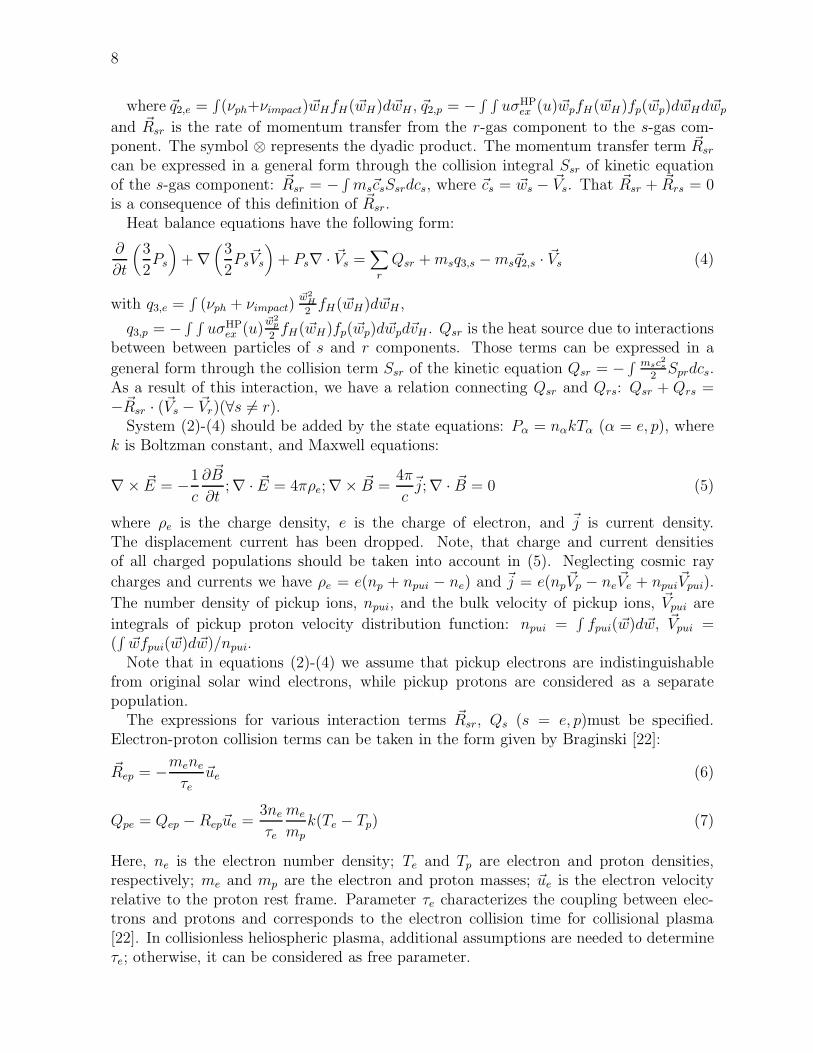
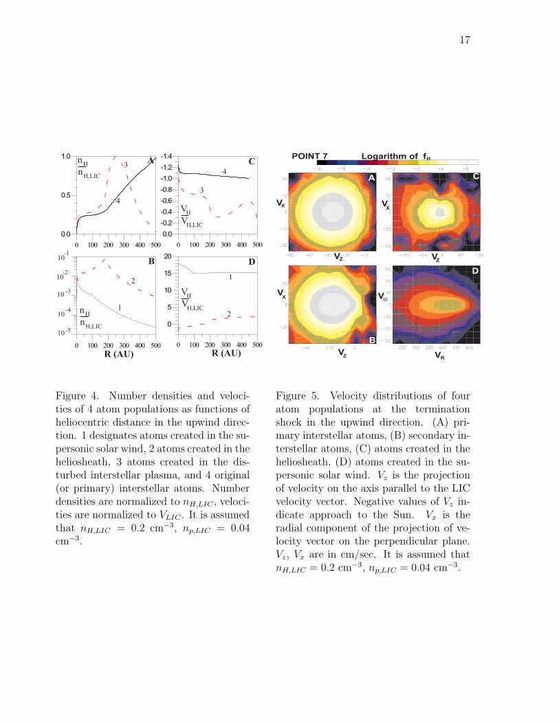
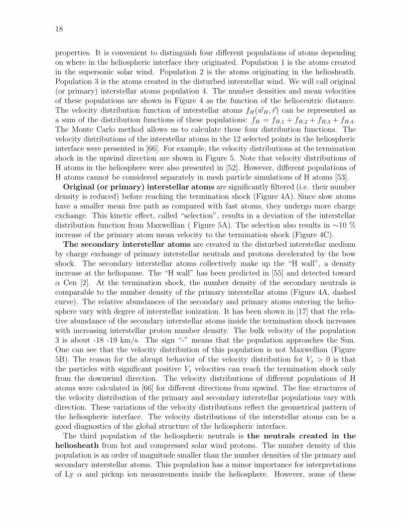
Figure 4. Number densities and veloci-ties of 4 atom populations as functions ofheliocentric distance in the upwind direc-tion. 1 designates atoms created in the su-personic solar wind, 2 atoms created in theheliosheath, 3 atoms created in the dis-turbed interstellar plasma, and 4 original(or primary) interstellar atoms. Numberdensities are normalized to nH,LIC , veloci-ties are normalized to VLIC . It is assumedthat nH,LIC = 0.2 cm−3, np,LIC = 0.04cm−3.

VV

V V

V V

V V

XX

X

Z Z

Z R

Θ

POINT 7 Logarithm of fH

A C

D

B

Figure 5. Velocity distributions of fouratom populations at the terminationshock in the upwind direction. (A) pri-mary interstellar atoms, (B) secondary in-terstellar atoms, (C) atoms created in theheliosheath, (D) atoms created in the su-personic solar wind. Vz is the projectionof velocity on the axis parallel to the LICvelocity vector. Negative values of Vz in-dicate approach to the Sun. Vx is theradial component of the projection of ve-locity vector on the perpendicular plane.Vz, Vx are in cm/sec. It is assumed thatnH,LIC = 0.2 cm−3, np,LIC = 0.04 cm−3.

18

properties. It is convenient to distinguish four different populations of atoms dependingon where in the heliospheric interface they originated. Population 1 is the atoms createdin the supersonic solar wind. Population 2 is the atoms originating in the heliosheath.Population 3 is the atoms created in the disturbed interstellar wind. We will call original(or primary) interstellar atoms population 4. The number densities and mean velocitiesof these populations are shown in Figure 4 as the function of the heliocentric distance.The velocity distribution function of interstellar atoms fH(~wH , ~r) can be represented asa sum of the distribution functions of these populations: fH = fH,1 + fH,2 + fH,3 + fH,4.The Monte Carlo method allows us to calculate these four distribution functions. Thevelocity distributions of the interstellar atoms in the 12 selected points in the heliosphericinterface were presented in [66]. For example, the velocity distributions at the terminationshock in the upwind direction are shown in Figure 5. Note that velocity distributions ofH atoms in the heliosphere were also presented in [52]. However, different populations ofH atoms cannot be considered separately in mesh particle simulations of H atoms [53].

Original (or primary) interstellar atoms are significantly filtered (i.e. their numberdensity is reduced) before reaching the termination shock (Figure 4A). Since slow atomshave a smaller mean free path as compared with fast atoms, they undergo more chargeexchange. This kinetic effect, called “selection”, results in a deviation of the interstellardistribution function from Maxwellian ( Figure 5A). The selection also results in ∼10 %increase of the primary atom mean velocity to the termination shock (Figure 4C).

The secondary interstellar atoms are created in the disturbed interstellar mediumby charge exchange of primary interstellar neutrals and protons decelerated by the bowshock. The secondary interstellar atoms collectively make up the “H wall”, a densityincrease at the heliopause. The “H wall” has been predicted in [55] and detected towardα Cen [2]. At the termination shock, the number density of the secondary neutrals iscomparable to the number density of the primary interstellar atoms (Figure 4A, dashedcurve). The relative abundances of the secondary and primary atoms entering the helio-sphere vary with degree of interstellar ionization. It has been shown in [17] that the rela-tive abundance of the secondary interstellar atoms inside the termination shock increaseswith increasing interstellar proton number density. The bulk velocity of the population3 is about -18 -19 km/s. The sign “-” means that the population approaches the Sun.One can see that the velocity distribution of this population is not Maxwellian (Figure5B). The reason for the abrupt behavior of the velocity distribution for Vz > 0 is thatthe particles with significant positive Vz velocities can reach the termination shock onlyfrom the downwind direction. The velocity distributions of different populations of Hatoms were calculated in [66] for different directions from upwind. The fine structures ofthe velocity distribution of the primary and secondary interstellar populations vary withdirection. These variations of the velocity distributions reflect the geometrical pattern ofthe heliospheric interface. The velocity distributions of the interstellar atoms can be agood diagnostics of the global structure of the heliospheric interface.

The third population of the heliospheric neutrals is the neutrals created in theheliosheath from hot and compressed solar wind protons. The number density of thispopulation is an order of magnitude smaller than the number densities of the primary andsecondary interstellar atoms. This population has a minor importance for interpretationsof Ly α and pickup ion measurements inside the heliosphere. However, some of these

19

atoms may probably be detected by Ly α hydrogen cell experiments due to their largeDoppler shifts. Due to their high energies, the particles influence the plasma distributionsin the LIC. Inside the termination shock the atoms propagate freely. Thus, these atomscan be the source of information on the plasma properties in the place of their birth, i.e.the heliosheath [6].

The last population of heliospheric atoms is the atoms created in the supersonicsolar wind. The number density of this atom population has a maximum at ∼5 AU.At this distance, the number density of population 1 is about two orders of magnitudesmaller than the number density of the interstellar atoms. Outside the termination shockthe density decreases faster than 1/r2 where r is the heliocentric distance (curve 1, Figure4B). The mean velocity of population 1 is about 450 km/sec, which corresponds to thebulk velocity of the supersonic solar wind. The velocity distribution of this populationis not Maxwellian either (Figure 5D). The extended “tail” in the distribution function iscaused by the solar wind plasma deceleration upstream of the termination shock. The“supersonic” atom population results in the plasma heating and deceleration upstream ofthe bow shock. This leads to the decrease of the Mach number ahead of the bow shock.

5.3. Recent developments in the Baranov-Malama modelThe Baranov-Malama model, the basic results of which were discussed above, takes into

account essentially two interstellar components: H atoms and charged particles. To applythis model to space experiments, one needs to evaluate how other possible componentsof the interstellar medium influence the results of this two-component model. Recently,several effects were taken into account in the frame of this axisymmetric model.

The influence of the galactic cosmic rays on the heliospheric interface structure wasstudied recently in [67], [68]. The study was done in the frame of two-component (plasmaand GCRs) and three-component (plasma, H atoms and GCRs) models. For the two-component case it was found that cosmic rays could considerably modify the shape andstructure of the solar wind termination shock and the bow shock and change the positionsof the heliopause and the bow shock. At the same time, for the three-component modelit was shown [68] that the GCR influence on the plasma flows is negligible as comparedwith the influence of H atoms. The exception is the bow shock, a structure that canbe strongly modified by the cosmic rays. It was also found ([49]; Alexashov, privatecommunication) that an anomalous component does not have a significant effect on theposition of the termination shock. However, ACRs may significantly reduce compressionat the termination shock [49].

Effects of the interstellar magnetic field on the plasma flow and on distribution of Hatoms in the interface were studied in [69] in the case of magnetic field parallel to therelative Sun/LIC velocity vector. In this case, the model remains axisymmetric. It wasshown that effects of the the interstellar magnetic field on the positions of the terminationand bow shocks and the heliopause are significantly smaller as compared to model withno atoms [29]. The calculations were performed with various Alfven Mach numbers in theundisturbed LIC. It was found that the bow shock straightens out with decreasing AlfvenMach number (increasing magnetic field strength in LIC). It approaches the Sun near thesymmetry axis, but recedes from it on the flanks. By contrast, the nose of the heliopauserecedes from the Sun due to tension of magnetic field lines, while the heliopause in its

20

wings approaches the Sun under magnetic pressure. As a result, the region of compressedinterstellar medium around the heliopause (or ”pileup region”) decreases by almost 30%, as the magnetic field increases from zero to 3.5 ×10−6 Gauss. It was also shownin [69] that H atom filtration and heliospheric distributions of primary and secondaryinterstellar atoms are virtually unchanged over the entire assumed range of the interstellarmagnetic field (0 - 3.5 ·10−6 Gauss). The magnetic field has the strongest effect on densitydistribution of population 2 of H atoms, which increases by a factor of almost 1.5 as theinterstellar magnetic field increases from zero to 3.5 · 10−6 Gauss.

Very recently a new non-stationary model of the solar wind interaction with two-component (H atoms and plasma) LIC was proposed in [70]. In this model the primaryand secondary interstellar atoms (populations 3 and 4) were treated as quasi-stationarykinetic gases. Population 1 of atoms originating in the supersonic solar wind was con-sidered as zero-pressure fluid. The calculations show that the qualitative features of thenon-stationary SW/LIC interaction established in [41] remain, but the effect of the solaractivity cycle is quantitatively stronger because the interface is closer to the Sun than inthe model with no atoms. The motion of the termination shock during the solar cycle onthe axis of symmetry is about 30 AU. Due to the solar cycle variations of the neutralizedsolar wind (i.e. atoms of population 1) the region between the heliopause and the bowshock widens and the mean plasma density in the region becomes smaller than for thestationary problem.

6. INTERPRETATIONS OF SPACECRAFT EXPERIMENTS ON THE BA-SIS OF THE BARANOV-MALAMA MODEL

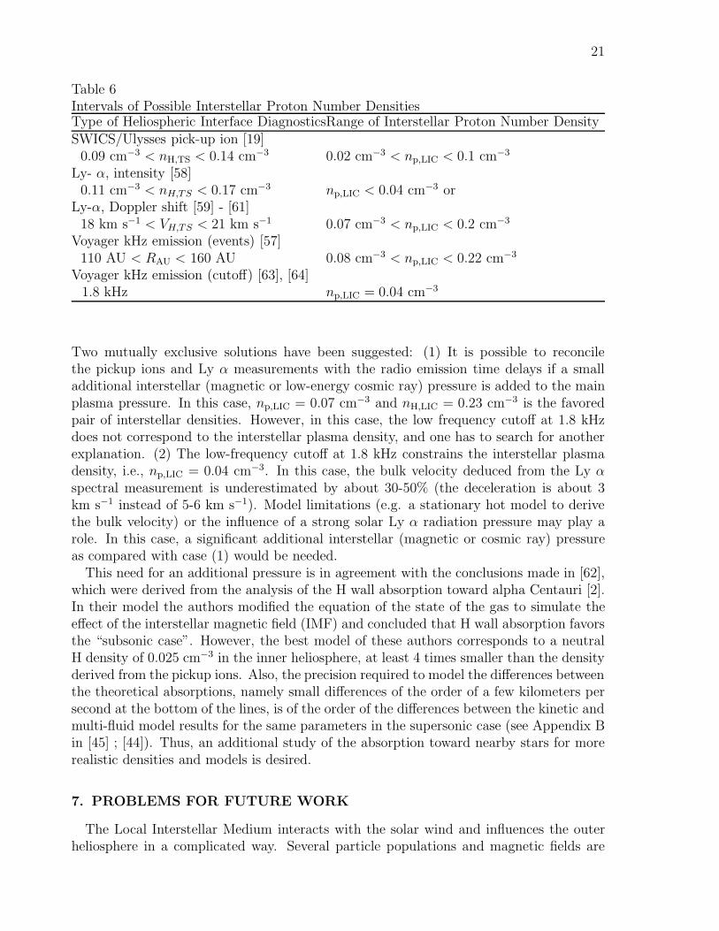
The Sun/LIC relative velocity and the LIC temperature are now well constrained ([13],[73]-[75]). Using the SWICS pickup He results and an interstellar HI/HeI ratio of 13± 1 (the average value of the ratio toward the nearby white dwarfs), Gloeckler et al.[19]concluded that nLIC(HI) = 0.2±0.03 cm −3. This estimation of nLIC(HI) is independentof the heliospheric interface model but model-dependent for determination of the numberdensity of H atoms from pickup fluxes. Estimates of interstellar electron number densityrequire a theoretical model of the heliospheric interface. The Baranov-Malama model wasused in [17] to study the sensitivity of the various types of indirect diagnostics of localinterstellar plasma density. The diagnostics are the degree of filtration, the temperatureand the velocity of the interstellar H atoms in the outer heliosphere (at the terminationshock), the distances to the termination shock, the heliopause, and the bow shock, andthe plasma frequencies in the LIC, at the bow shock and in the maximum compressionregion around the heliopause, which constitutes the “barrier” for radio waves formedin the interstellar medium. We also searched [17] for a number density of interstellarprotons compatible with SWICS/Ulysses pickup ion observations, backscattered solar Lyα observed by SOHO, Voyager and HST, and kHz radiations observed by Voyager. Table1 presents the ranges of np,LIC obtained on the basis of the Baranov-Malama model andcomparable to these observations.

From analysis of the ranges, it was concluded in [17] that it is difficult in the frame of themodel to reconcile the results obtained from all types of data as they stand now. Thereis a need for some modifications of the interpretations or of the confidence intervals.

21

Table 6Intervals of Possible Interstellar Proton Number DensitiesType of Heliospheric Interface DiagnosticsRange of Interstellar Proton Number DensitySWICS/Ulysses pick-up ion [19]

0.09 cm−3 < nH,TS < 0.14 cm−3 0.02 cm−3 < np,LIC < 0.1 cm−3

Ly- α, intensity [58]0.11 cm−3 < nH,TS < 0.17 cm−3 np,LIC < 0.04 cm−3 or

Ly-α, Doppler shift [59] - [61]18 km s−1 < VH,TS < 21 km s−1 0.07 cm−3 < np,LIC < 0.2 cm−3

Voyager kHz emission (events) [57]110 AU < RAU < 160 AU 0.08 cm−3 < np,LIC < 0.22 cm−3

Voyager kHz emission (cutoff) [63], [64]1.8 kHz np,LIC = 0.04 cm−3

Two mutually exclusive solutions have been suggested: (1) It is possible to reconcilethe pickup ions and Ly α measurements with the radio emission time delays if a smalladditional interstellar (magnetic or low-energy cosmic ray) pressure is added to the mainplasma pressure. In this case, np,LIC = 0.07 cm−3 and nH,LIC = 0.23 cm−3 is the favoredpair of interstellar densities. However, in this case, the low frequency cutoff at 1.8 kHzdoes not correspond to the interstellar plasma density, and one has to search for anotherexplanation. (2) The low-frequency cutoff at 1.8 kHz constrains the interstellar plasmadensity, i.e., np,LIC = 0.04 cm−3. In this case, the bulk velocity deduced from the Ly αspectral measurement is underestimated by about 30-50% (the deceleration is about 3km s−1 instead of 5-6 km s−1). Model limitations (e.g. a stationary hot model to derivethe bulk velocity) or the influence of a strong solar Ly α radiation pressure may play arole. In this case, a significant additional interstellar (magnetic or cosmic ray) pressureas compared with case (1) would be needed.

This need for an additional pressure is in agreement with the conclusions made in [62],which were derived from the analysis of the H wall absorption toward alpha Centauri [2].In their model the authors modified the equation of the state of the gas to simulate theeffect of the interstellar magnetic field (IMF) and concluded that H wall absorption favorsthe “subsonic case”. However, the best model of these authors corresponds to a neutralH density of 0.025 cm−3 in the inner heliosphere, at least 4 times smaller than the densityderived from the pickup ions. Also, the precision required to model the differences betweenthe theoretical absorptions, namely small differences of the order of a few kilometers persecond at the bottom of the lines, is of the order of the differences between the kinetic andmulti-fluid model results for the same parameters in the supersonic case (see Appendix Bin [45] ; [44]). Thus, an additional study of the absorption toward nearby stars for morerealistic densities and models is desired.

7. PROBLEMS FOR FUTURE WORK

The Local Interstellar Medium interacts with the solar wind and influences the outerheliosphere in a complicated way. Several particle populations and magnetic fields are

22

involved in this interaction. From the interstellar side, the interacting populations are theplasma (electron and proton) component, H atom component, interstellar magnetic field,and galactic cosmic rays. Heliospheric plasma consists of original solar wind protons,electrons, pickup protons, and the anomalous component of cosmic rays. A large efforthas been done to study the theoretical physics of the interaction region. However, acomplete, self-consistent model of the heliospheric interface has not yet been constructed,because of the difficulty connecting both the multi-fluid nature of the heliosphere andthe requirements of the different theoretical approaches for different components of theinteraction. Many aspects were studied and reported here in previous sections. However,some aspects require additional theoretical explorations. Most theoretical models employthe one-fluid approach for solar wind and interstellar plasmas. It has been shown that, toderive one-fluid approach equations, several assumptions are needed. A key assumptionthat looks reasonable is co-moving character of all components. Another assumption fora one-fluid plasma model is the immediate assimilation of the pickup ion component intothe solar wind. As demonstrated by space experiments, this is not the case and it wouldbe more natural to consider solar protons and pickup protons separately as co-movingpopulations. The electron component should also be treated as a distinct population.However, since the assumption of the co-moving character of these three heliosphericplasma populations looks reasonable, the one-fluid approach gives us a reasonably accuratepicture of the flow pattern (positions of the shocks and heliopause) and plasma velocitydistributions. Theoretical models of pickup ion acceleration and diffusion can be employedto determine the distribution of thermal energy between solar wind and pickup protoncomponents. A similar study should be done for electrons.

Another important aspect of the solar/wind interaction is a study of the tail regionof the solar wind and interstellar medium interaction. Although some studies were done([76], [77]) it is still not clear at which heliocentric distances the gas (plasma and H atoms)parameters become indistinguishable from local interstellar parameters, or in other words,how far signatures of the solar system are noticeable in the interstellar medium. It is stillnot clear which of the two competiting processes is the most important in the tail region- charge exchange or plasma transport across the heliopause due to different instabilities.Studies of Saturn’s and Earth’s magnetic tails show that such tails can be very extended[78], [79].

Finally, growing interest in heliospheric interface studies is connected with expectationsthat Voyager 1 will cross the termination shock soon. Many predictions of the time of thetermination shock crossing by Voyager appeared in the literature. However, it seems thatmuch more work should be done to explain and reconcile all available indirect observationsof the heliospheric interface based on the unique model of the heliospheric interface. Thiswork should be done especially because NASA plans to send a spacecraft to a heliocentricdistance of at least 200 AU with a flight-time of only 10 or 15 years. Intensive theoreticalstudy will help to optimize goals, instrumentation, and, finally, the scientific profit of this”interstellar” mission.

Acknowledgements. This work was supported in part by CRDF Award RP1-2248,INTAS Award 2001-0270, YSF 00-163, RFBR grants 01-02-17551, 02-02-06011, 01-01-00759, and the International Space Science Institute in Bern. I thank V. B. Baranov andS. V. Chalov for useful discussions.

23

REFERENCES

1. R. von Steiger, R. Lallement, and M. A. Lee (eds.), The Heliosphere in the LocalInterstellar Medium, Hardbound, 1996.

2. Linsky, J., Wood, B., Astrophys. J. 463 (1996), 254.3. Wood, B. E., Muller, H.; Zank, G. P., Astrophys. J. 542 (2000), 493-503.4. Izmodenov, V., Lallement, R., Malama, Y., Astron. Astrophys. 342 (1999), L13-L16.5. Izmodenov, V., Wood, B., Lallement, R., J. Geophys. Res., in press, 2002.6. Gruntman et al., J. Geophys. Res. 106, 15767-15782 (2001).7. Parker, E. N., Astrophys. J. 134 (1961), 20-27.8. Baranov, V.B., Krasnobaev, K.V., Kulikovksy, A.G., Sov. Phys. Dokl. 15 (1971), 791.9. Fichtner, H., Space Sci. Rev. 95 (2001), 639-754.10. Zank, G., Space Sci. Rev. 89 (1999), 413-688.11. Richardson, J.D., The Outer Heliosphere: The Next Frontiers, Edited by K. Scherer,

H. Fichtner, H. Fahr, and E. Marsch, COSPAR Colloquiua Series, 11. Amsterdam:Pergamon Press (2001), 301-310.

12. Lallement, R., Space Sci. Rev. 78 (1996), 361-374.13. Witte, M., Banaszkiewicz, M.; Rosenbauer, H., Space Sci. Rev. 78 (1996), 289-296.14. Gloeckler, Space Sci. Rev. 78 (1996), 335-346.15. Moebius, E., Space Sci. Rev. 78 (1996), 375-386.16. Baranov, V. B., Malama, Y. G., J. Geophys. Res. 100 (1995), 14,755-14,762.17. Izmodenov V., Geiss, J., Lallement, R., et al., J. Geophys. Res. (1999), 4731-4742.18. Webber, W.R., Lockwood, J., McDonald, F., Heikkila, B., J. Geophys. Res. 106

(2001), 253-260.19. Gloeckler, Nature 386 (1997), 374-377.20. Izmodenov, V., Malama, Y., Kalinin, A.,et al., Astrophys. Space Sci. 274 (2000),

71-76.21. Baranov, V. B., Astrophys. Space Sci. 274 (2000), 3-16.22. Braginski, S.I., Voprosy teorii plasmy, v.1, Atomizdat, Moscow, 1963 (in russian).23. Isenberg, P., J. Geophys. Res. 102 (1997), 4719-4724.24. Chalov, S. V., Fahr, H., Astron. Astrophys., 335 (1998), 746-756.25. Williams, L., Zank, G., Matthaeus, W., J. Geophys. Res. 100 (1995), 17059-17068.26. Chalov, S. V., Fahr, H., Astron. Astrophys. 311 (1996), 317-328.27. Chalov, S. V., Fahr, H., Astron. Astrophys. 326 (1997), 860-869.28. Fujimoto Y., Matsuda, T., Preprint No. KUGD91-2, Kobe Univ., Japan, 1991.29. Baranov, V.B., Zaitsev, N.A., Astron. Astrophys. 304 (1995), 631.30. Pogorelov, N., Semenov, A., Astron. Astrophys. 321 (1997), 330.31. Myasnikov, A., Preprint No. 585, Institute for Problems in Mechanics, Russian

Academy of Sciences, 1997.32. Ratkiewicz, R., Barnes, A, et al., Astron. Astrophys. 335 (1998), 363.33. Pogorelov, N., Matsuda, T., J. Geophys. Res. 103 (1998), 237-245.34. Linde, T., Gombosi, T., Roe, P., J. Geophys. Res. 103 (1998), 1889-1904.35. Tanaka, T., Washimi, H., J. Geophys. Res. 104 (1999), 12605.36. Ratkiewicz, R., Barnes, A., J. Spreiter, J. Geophys. Res. 105 (2000), 25,021-25,031.37. Pauls, H. and G. Zank, J. Geophys. Res. 102 (1997), 19779-19788.

24

38. Steinolfson, R.S., J. Geophys. Res. 99 (1994), 13,307-13,314.39. Pogorelov, N., Astron. Astrophys. 297 (1995), 835.40. Karmesin, S., Liewer, P, Brackbill, J., Geophys. Res. Let. 22 (1995), 1153-1163.41. Baranov, V., Zaitsev, N., Geophys. Res. Let. 25 (1998), 4051.42. Wang, C., Belcher, J, J. Geophys. Res. 104 (1999), 549-556.43. Zank, G., Pauls, H., Williams, L., Hall, D., J. Geophys. Res. 101 (1996), 21639-21656.44. Baranov, V. B., Izmodenov, V., Malama, Y., J. Geophys. Res. 103 (1998), 9575-9586.45. Williams, L., Hall, D. T., Pauls, H. L., Zank, G. P., Astrophys. J. 476 (1997), 366.46. Liewer, P., Brackbill, J., Karmesin, S., International Solar Wind 8 Conference, p.33,

1995.47. McNutt, R., Lyon, J., Goodrich, C., J. Geophys. Res. 103 (1998), 1905.48. McNutt, R., Lyon, J., Goodrich, C., J. Geophys. Res. 104 (1999), 14803.49. Fahr, H., Kausch, T., Scherer, H., Astron. Astrophys. 357 (2000), 268-282.50. Osterbart, R., and H. Fahr, Astron. Astrophys. 264 (1992), 260-269.51. Baranov, V., Malama, Y., J. Geophys. Res. 98 (1993), 15157.52. Muller et al., J. Geophys. Res., 27,419-27,438 (2000)53. Lipatov et al., J. Geophys Res., 1998.54. Baranov, V. B., and Y. G. Malama, Space Sci. Rev. 78 (1996), 305-316.55. Baranov, V. B., Lebedev, M.,Malama Y., Astrophys. J. 375 (1991), 347-351.56. Malama, Y. G., Astrophys. Space Sci., 176 (1991), 21-46.57. Gurnett, D.,Kurth,W.,Space Sci. Rev. 78 (1996), 53-66.58. Quemerais, E., Bertaux, J.-L., Sandel, B., Lallement, R., Astron. Astrophys. 290

(1994), 941-955.59. Bertaux, J.-L., Lallement, R., Kurt, V., Mironova,E. N., Astron. Astrophys. 150

(1985), 1-20.60. Lallement, R., Linsky, J., Lequeux, J., Baranov, V., Space Sci. Rev. 78 (1996), 299-

304.61. Clarke, J., Lallement, R., Quemerais, E., Bertaux, J.-L., Scherer, H., Astron. Astro-

phys. 499 (1998), 482.62. Gayley, K., Zank G. P., et al., Astron. Astrophys. 487 (1997), 259.63. Gurnett, D. A., Kurth, W., Allendorf, S., Poynter, R., Science 262 (1993), 199-202.64. Grzedzielski, S., Lallement, R., Space Sci. Rev. 78 (1996), 247-258.65. Treumann, R., Macek, W., Izmodenov, V, Astron. Astrophys. 336 (1998), L45.66. Izmodenov, V., Gruntman, M., Malama, Y., J. Geophys. Res. 106 (2001), 10681.67. Myasnikov, Izmodenov, V., Alexashov, D., Chalov, S., J. Geophys. Res. 105 (2000),

5179.68. Myasnikov, Alexashov, D., Izmodenov, V., Chalov, S., J. Geophys. Res. 105 (2000),

5167.69. Aleksashov, D., Baranov, V., Barsky, E., Myasnikov, A., Astronomy Letters 26 (2000),

743-749.70. Zaitsev, N., Izmodenov V., in The Outer Heliosphere: The Next Frontiers, Edited

by K. Scherer, H. Fichtner, H. Fahr, and E. Marsch, COSPAR Colloquiua Series, 11.Amsterdam: Pergamon Press (2001), 65-69.

71. Isenberg, P., J. Geophys. Res. 91 (1986), 9965.72. Holzer, J. Geophys. Res. 77 (1972), 5407.

25

73. Lallement R., Bertin, Astron. Astrophys. 266 (1992), 479-485.74. Linsky, J., Brown A., Gayley, K., et al., Astron. J. 402 (1993), 694-709.75. Lallement, R., Ferlet, A., et al., Astron. Astrophys. 304 (1995), 461-474.76. Jaeger, Fahr, H., Solar Physics, 178 (1998),631-656.77. Fahr, H., Neutsch, W., Grzedzielski, S., et al., Space Sci. Rev 43 (1986) 329-381.78. Grzedzielski, S., Macek, W., Obrec, P., Nature, 292 (1981) 615-616.79. Grzedzielski, S., Macek, W., J. Geophys. Res. 93 (1988), 1795-1808.