Models of effective connectivity & Dynamic Causal Modelling (DCM) Klaas Enno Stephan Laboratory for Social & Neural Systems Research Institute for Empirical

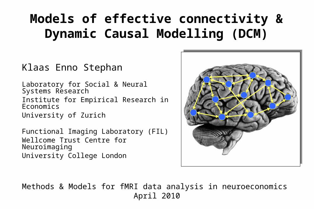
Models of effective connectivity &Dynamic Causal Modelling (DCM)

Klaas Enno Stephan

Laboratory for Social & Neural Systems Research Institute for Empirical Research in EconomicsUniversity of Zurich

Functional Imaging Laboratory (FIL)Wellcome Trust Centre for NeuroimagingUniversity College London

Methods & Models for fMRI data analysis in neuroeconomics April 2010

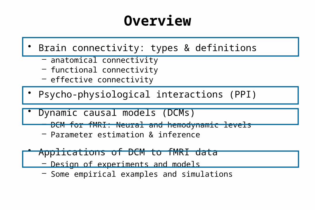
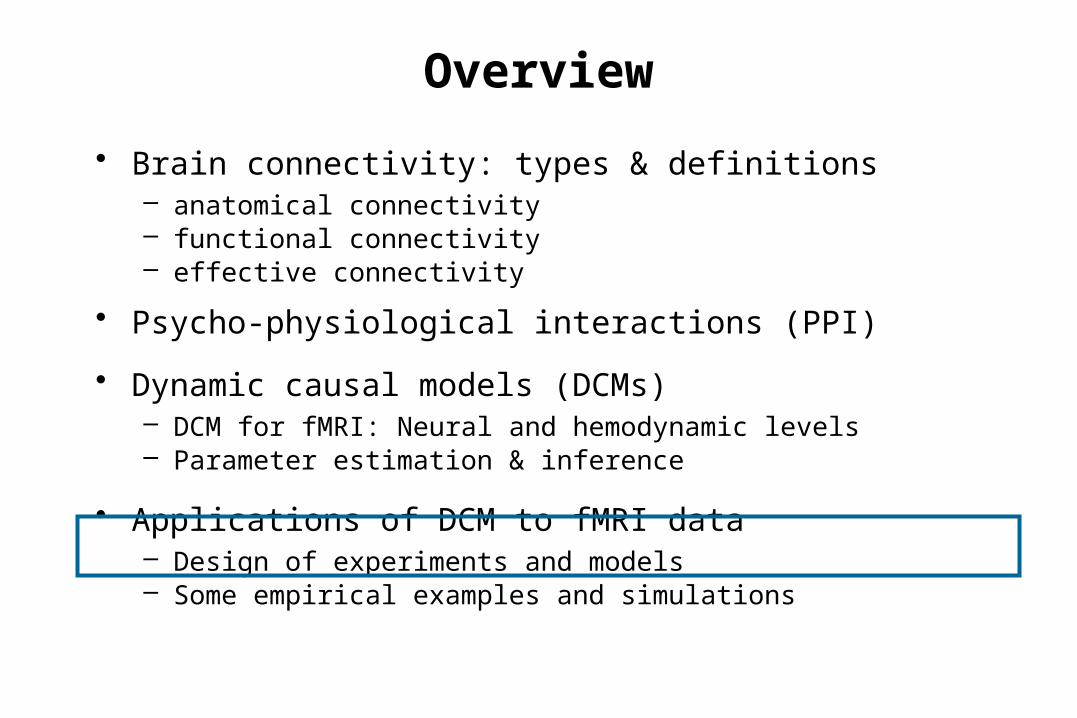
Overview

• Brain connectivity: types & definitions– anatomical connectivity– functional connectivity– effective connectivity

• Psycho-physiological interactions (PPI)

• Dynamic causal models (DCMs)– DCM for fMRI: Neural and hemodynamic levels– Parameter estimation & inference

• Applications of DCM to fMRI data– Design of experiments and models– Some empirical examples and simulations

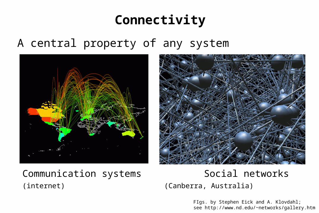
Connectivity

A central property of any system

Communication systems Social networks(internet) (Canberra, Australia)

FIgs. by Stephen Eick and A. Klovdahl;see http://www.nd.edu/~networks/gallery.htm

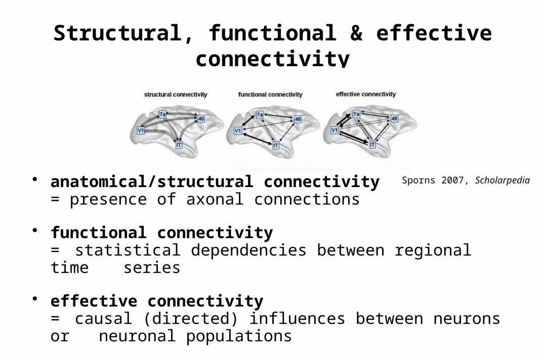
Structural, functional & effective connectivity

• anatomical/structural connectivity= presence of axonal connections

• functional connectivity = statistical dependencies between regional time series

• effective connectivity = causal (directed) influences between neurons or neuronal populations

Sporns 2007, Scholarpedia

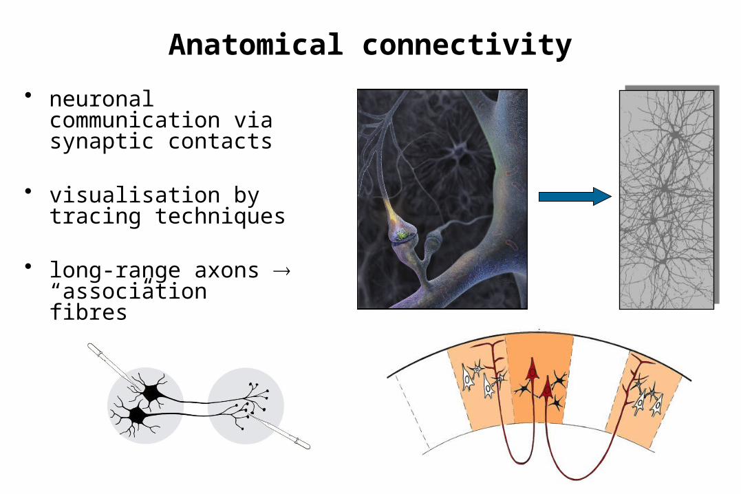
Anatomical connectivity

• neuronal communication via synaptic contacts

• visualisation by tracing techniques

• long-range axons “association fibres”

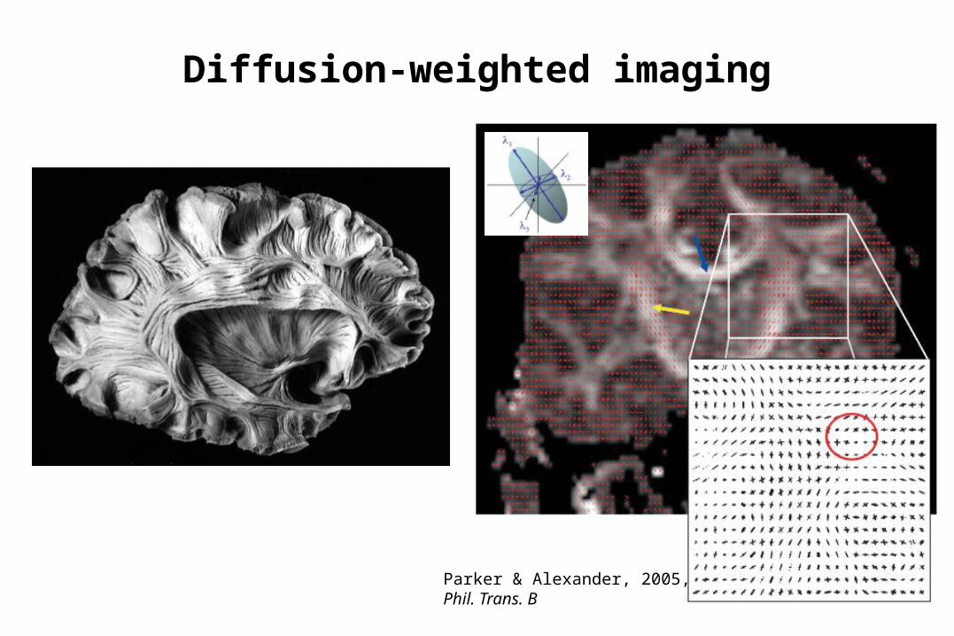
Diffusion-weighted imaging

Parker & Alexander, 2005, Phil. Trans. B

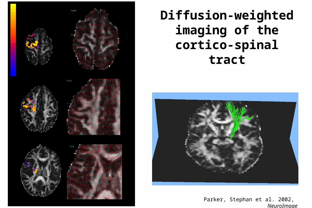
Parker, Stephan et al. 2002, NeuroImage

Diffusion-weighted imaging of the

cortico-spinal tract

Why would complete knowledge of anatomical connectivity not be enough

to understand how the brain works?

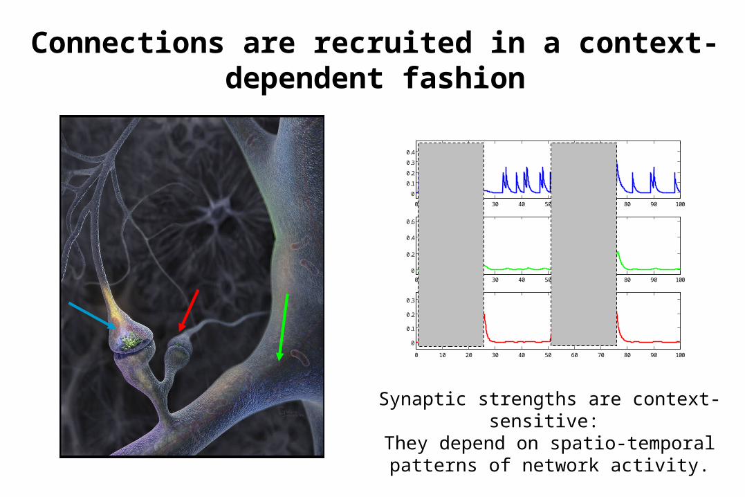
Connections are recruited in a context-dependent fashion

0 10 20 30 40 50 60 70 80 90 100

0

0.1

0.2

0.3

0.4

0 10 20 30 40 50 60 70 80 90 100

0

0.2

0.4

0.6

0 10 20 30 40 50 60 70 80 90 100

0

0.1

0.2

0.3

Synaptic strengths are context-sensitive: They depend on spatio-temporal patterns

of network activity.

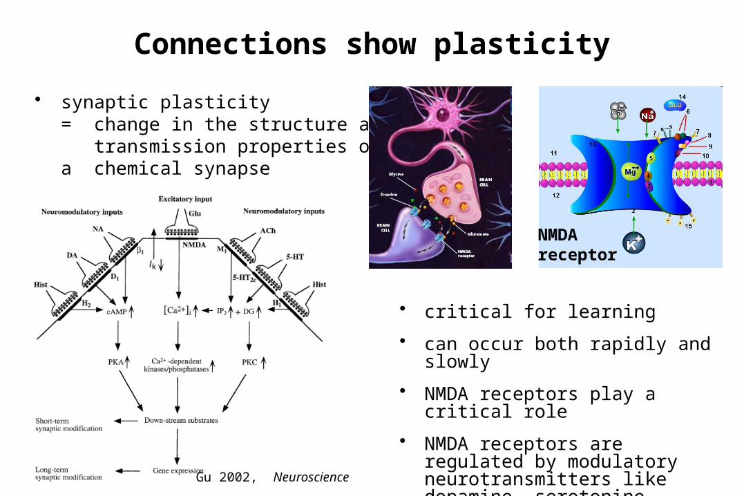
Connections show plasticity

• critical for learning

• can occur both rapidly and slowly

• NMDA receptors play a critical role

• NMDA receptors are regulated by modulatory neurotransmitters like dopamine, serotonine, acetylcholine

• synaptic plasticity = change in the structure and transmission properties of a chemical synapse

Gu 2002, Neuroscience

NMDAreceptor

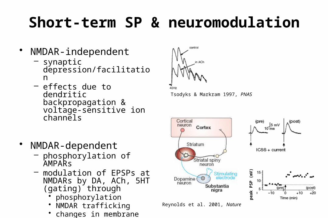
Short-term SP & neuromodulation

• NMDAR-independent– synaptic

depression/facilitation– effects due to dendritic

backpropagation & voltage-sensitive ion channels

• NMDAR-dependent– phosphorylation of AMPARs– modulation of EPSPs at

NMDARs by DA, ACh, 5HT (gating) through• phosphorylation• NMDAR trafficking• changes in membrane

potential

Reynolds et al. 2001, Nature

Tsodyks & Markram 1997, PNAS

pea

k P

SP

(m

V)

Different approaches to analysing functional connectivity

• Seed voxel correlation analysis

• Eigen-decomposition (PCA, SVD)

• Independent component analysis (ICA)

• any other technique describing statistical dependencies amongst regional time series

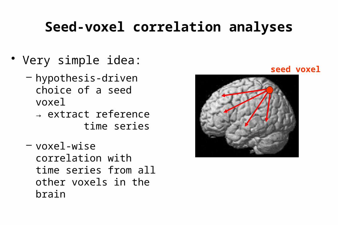
Seed-voxel correlation analyses

• Very simple idea:– hypothesis-driven choice of

a seed voxel → extract reference

time series

– voxel-wise correlation with time series from all other voxels in the brain

seed voxel

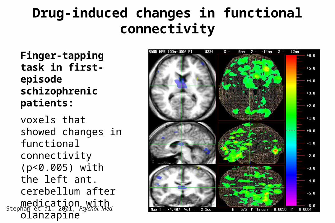
Drug-induced changes in functional connectivity

Finger-tapping task in first-episode schizophrenic patients:

voxels that showed changes in functional connectivity (p<0.005) with the left ant. cerebellum after medication with olanzapineStephan et al. 2001, Psychol. Med.

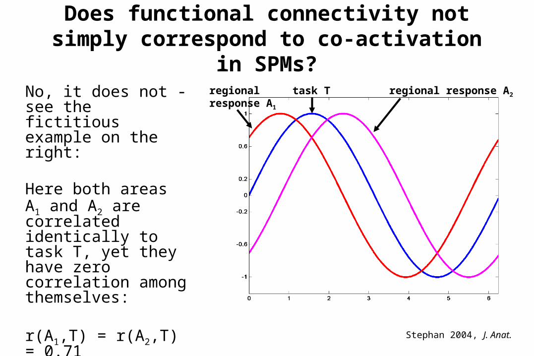
Does functional connectivity not simply correspond to co-activation in

SPMs?No, it does not - see the fictitious example on the right:

Here both areas A1 and A2 are correlated identically to task T, yet they have zero correlation among themselves:

r(A1,T) = r(A2,T) = 0.71butr(A1,A2) = 0 !

task T regional response A2regional response A1

Stephan 2004, J. Anat.

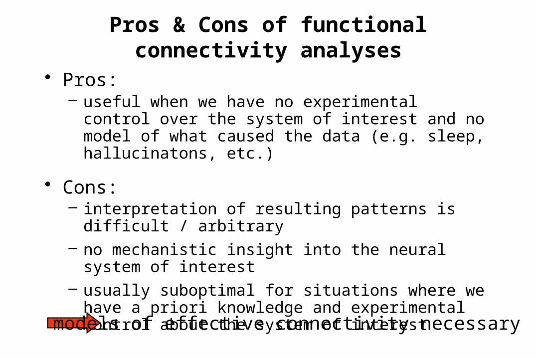
Pros & Cons of functional connectivity analyses

• Pros:– useful when we have no experimental control over

the system of interest and no model of what caused the data (e.g. sleep, hallucinatons, etc.)

• Cons:– interpretation of resulting patterns is difficult /

arbitrary – no mechanistic insight into the neural system of

interest– usually suboptimal for situations where we have a

priori knowledge and experimental control about the system of interestmodels of effective connectivity necessary

For understanding brain function mechanistically, we need models of effective connectivity, i.e.

models of causal interactions among neuronal populations.

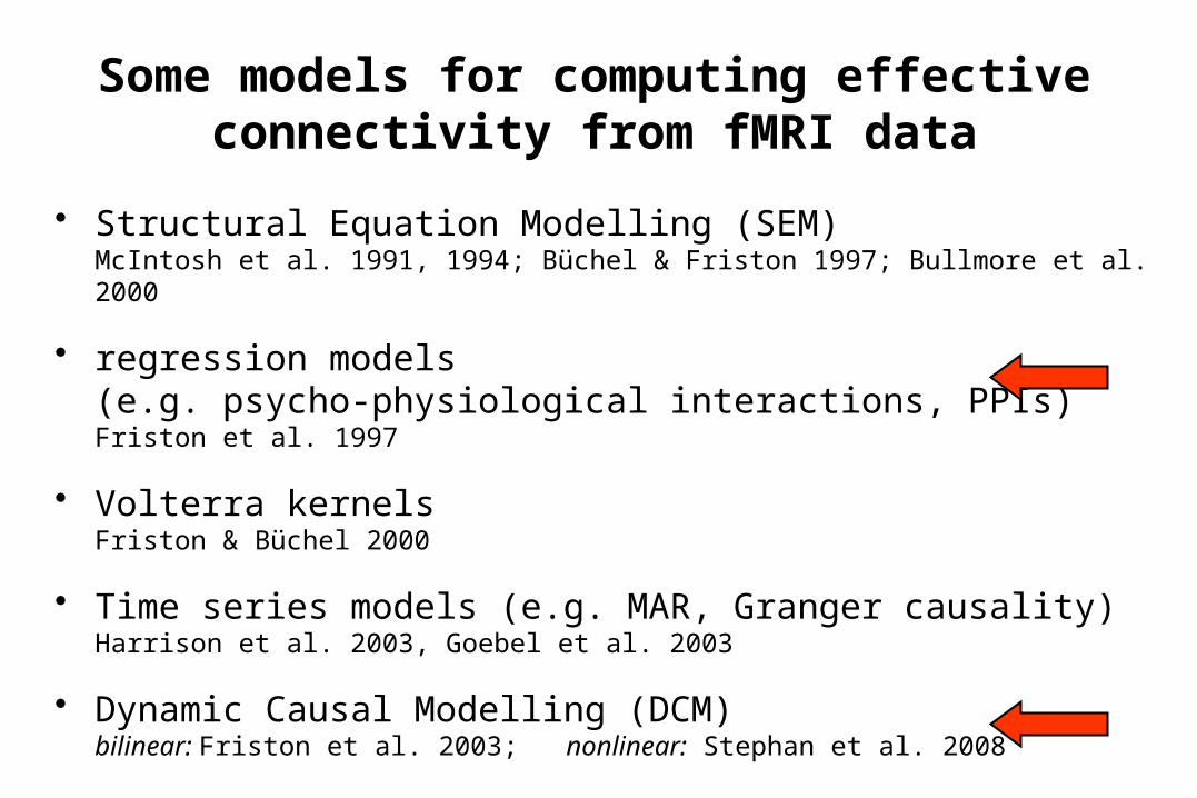
Some models for computing effective connectivity from fMRI data

• Structural Equation Modelling (SEM) McIntosh et al. 1991, 1994; Büchel & Friston 1997; Bullmore et al. 2000

• regression models (e.g. psycho-physiological interactions, PPIs)Friston et al. 1997

• Volterra kernels Friston & Büchel 2000

• Time series models (e.g. MAR, Granger causality)Harrison et al. 2003, Goebel et al. 2003

• Dynamic Causal Modelling (DCM)bilinear: Friston et al. 2003; nonlinear: Stephan et al. 2008

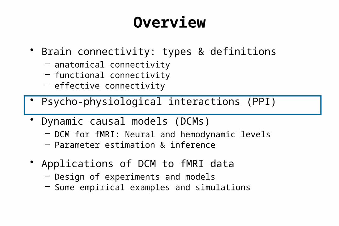
Overview





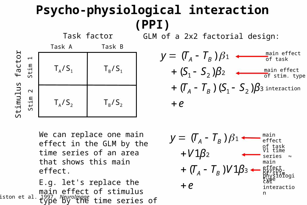
Psycho-physiological interaction (PPI)

We can replace one main effect in the GLM by the time series of an area that shows this main effect.

E.g. let's replace the main effect of stimulus type by the time series of area V1:

Task factorTask A Task B

Sti

m 1

Sti

m 2

Sti

mu

lus

fact

or

TA/S1 TB/S1

TA/S2 TB/S2

e

βVTT

βV

TT y

BA

BA

3

2

1

1 )(

1

)(

e

βSSTT

βSS

TT y

BA

BA

321

221

1

)( )(

)(

)(

GLM of a 2x2 factorial design:

main effectof task

main effectof stim. type

interaction

main effectof taskV1 time series main effectof stim. typepsycho-physiologicalinteraction

Friston et al. 1997, NeuroImage

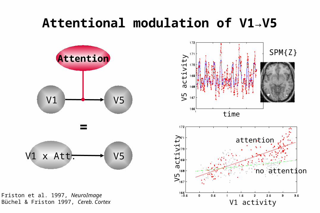
V1

attention

no attention

V1 activity

V5 a

ctiv

ity

SPM{Z}

time

V5 a

ctiv

ity

Friston et al. 1997, NeuroImageBüchel & Friston 1997, Cereb. Cortex

V1 x Att.

=

V5

V5

Attention

Attentional modulation of V1→V5

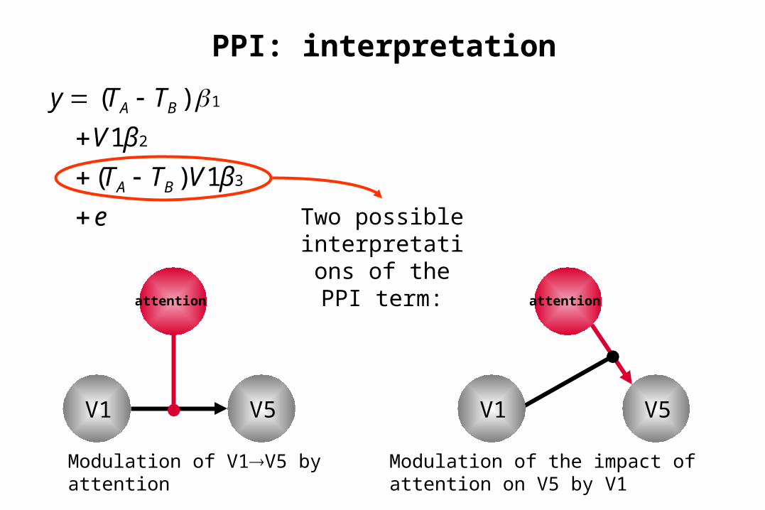
PPI: interpretation

Two possible interpretations

of the PPI term:

V1

Modulation of V1V5 by attention

Modulation of the impact of attention on V5 by V1

V1 V5 V1

V5

attention

V1

attention

e

βVTT

βV

TT y

BA

BA

3

2

1

1 )(

1

)(

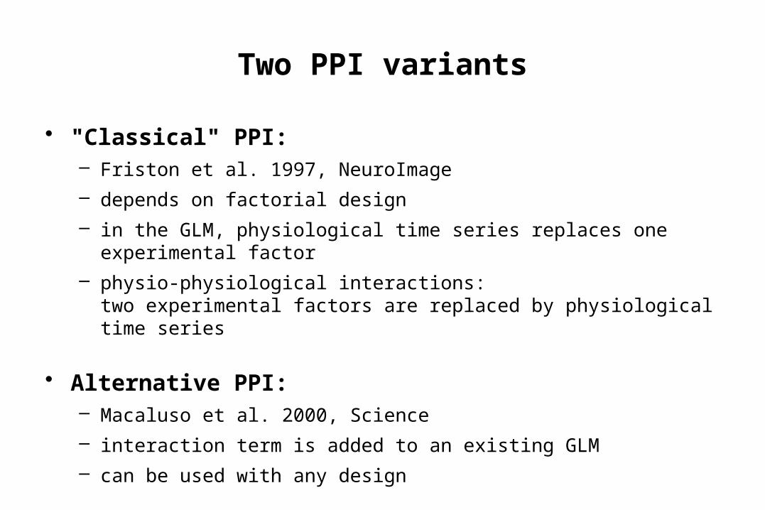
Two PPI variants

• "Classical" PPI: – Friston et al. 1997, NeuroImage

– depends on factorial design

– in the GLM, physiological time series replaces one experimental factor

– physio-physiological interactions: two experimental factors are replaced by physiological time series

• Alternative PPI:– Macaluso et al. 2000, Science

– interaction term is added to an existing GLM

– can be used with any design

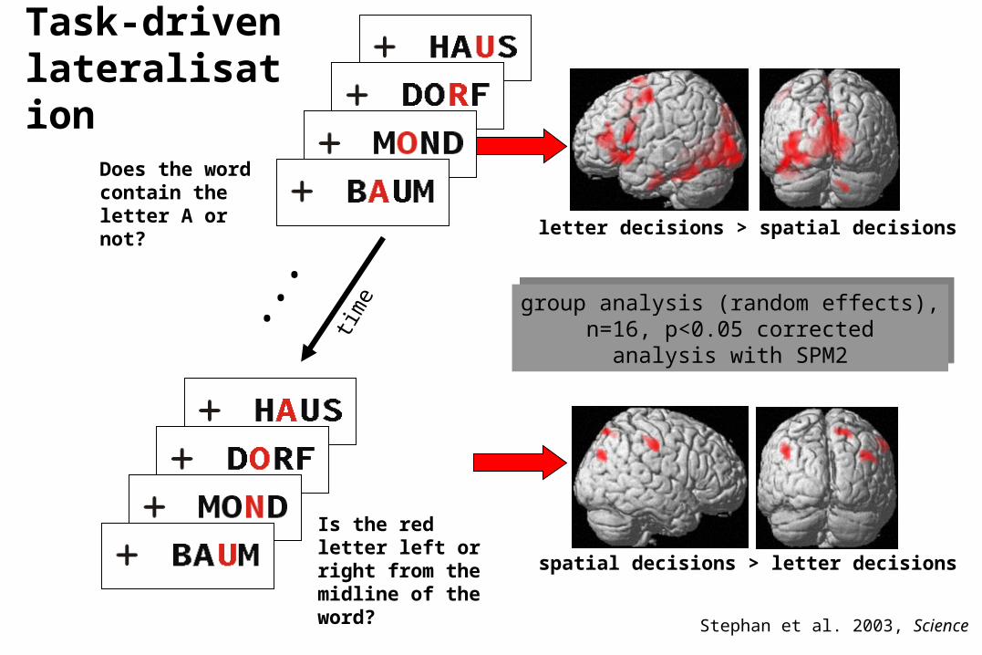
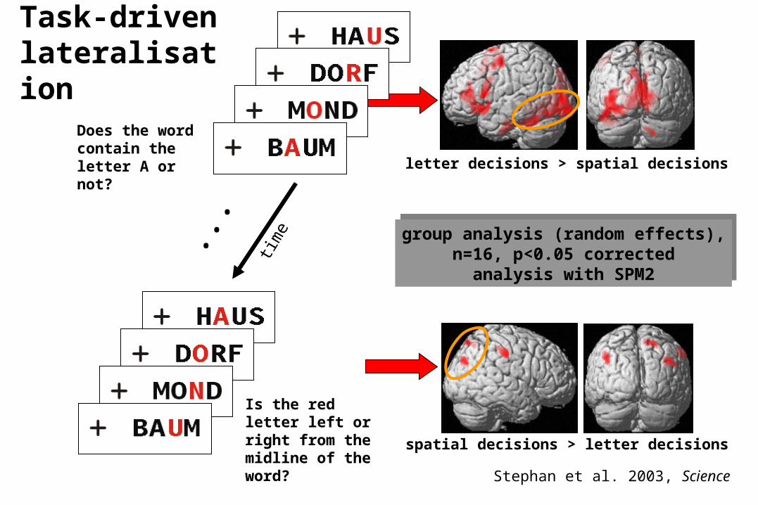
Is the red letter left or right from the midline of the word?

group analysis (random effects),n=16, p<0.05 corrected

analysis with SPM2


analysis with SPM2

Task-driven lateralisation

letter decisions > spatial decisions

time

•••

Does the word contain the letter A or not?

spatial decisions > letter decisions

Stephan et al. 2003, Science

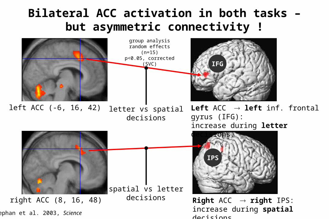
Bilateral ACC activation in both tasks –but asymmetric connectivity !

IPS

IFG

Left ACC left inf. frontal gyrus (IFG):increase during letter decisions.

Right ACC right IPS:increase during spatial decisions.

left ACC (-6, 16, 42)

right ACC (8, 16, 48)

spatial vs letterdecisions

letter vs spatialdecisions

group analysisrandom effects (n=15)

p<0.05, corrected (SVC)


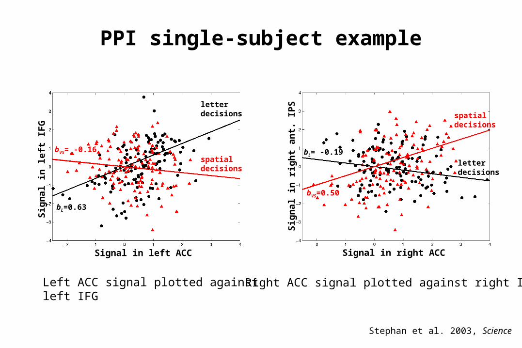
PPI single-subject example

bVS= -0.16

bL=0.63

Signal in left ACC

Sig

nal

in

lef

t IF

G

bL= -0.19

Sig

nal

in

rig

ht

ant.

IP

S

Signal in right ACC

bVS=0.50

Left ACC signal plotted against left IFG

spatialdecisions

letterdecisions

letterdecisions

spatialdecisions

Right ACC signal plotted against right IPS


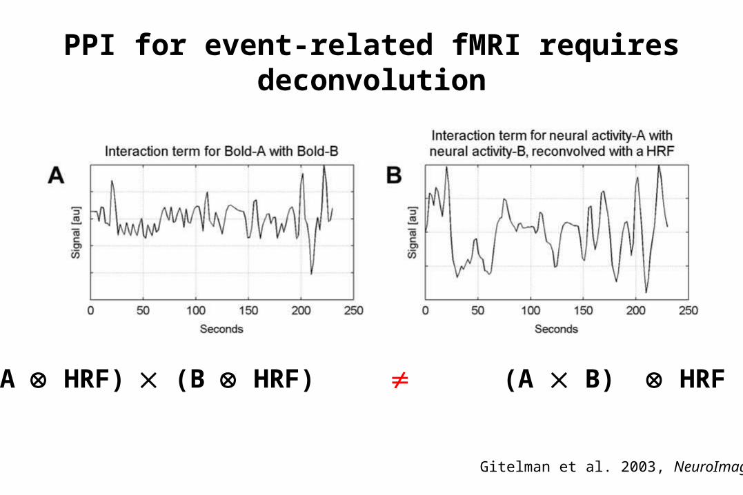
PPI for event-related fMRI requires deconvolution

Gitelman et al. 2003, NeuroImage

(A HRF) (B HRF) (A B) HRF

Pros & Cons of PPIs• Pros:

– given a single source region, we can test for its context-dependent connectivity across the entire brain

– easy to implement

• Cons:– very simplistic model:

only allows to model contributions from a single area

– ignores time-series properties of data

– application to event-related data relies deconvolution procedure (Gitelman et al. 2003, NeuroImage)

– operates at the level of BOLD time series

sometimes very useful, but limited causal interpretability;in most cases, we need more powerful models

Overview





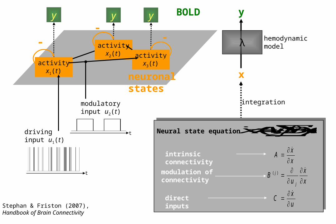
Dynamic causal modelling (DCM)

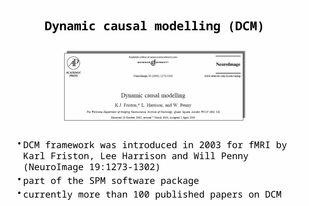
• DCM framework was introduced in 2003 for fMRI by Karl Friston, Lee Harrison and Will Penny (NeuroImage 19:1273-1302)• part of the SPM software package• currently more than 100 published papers on DCM

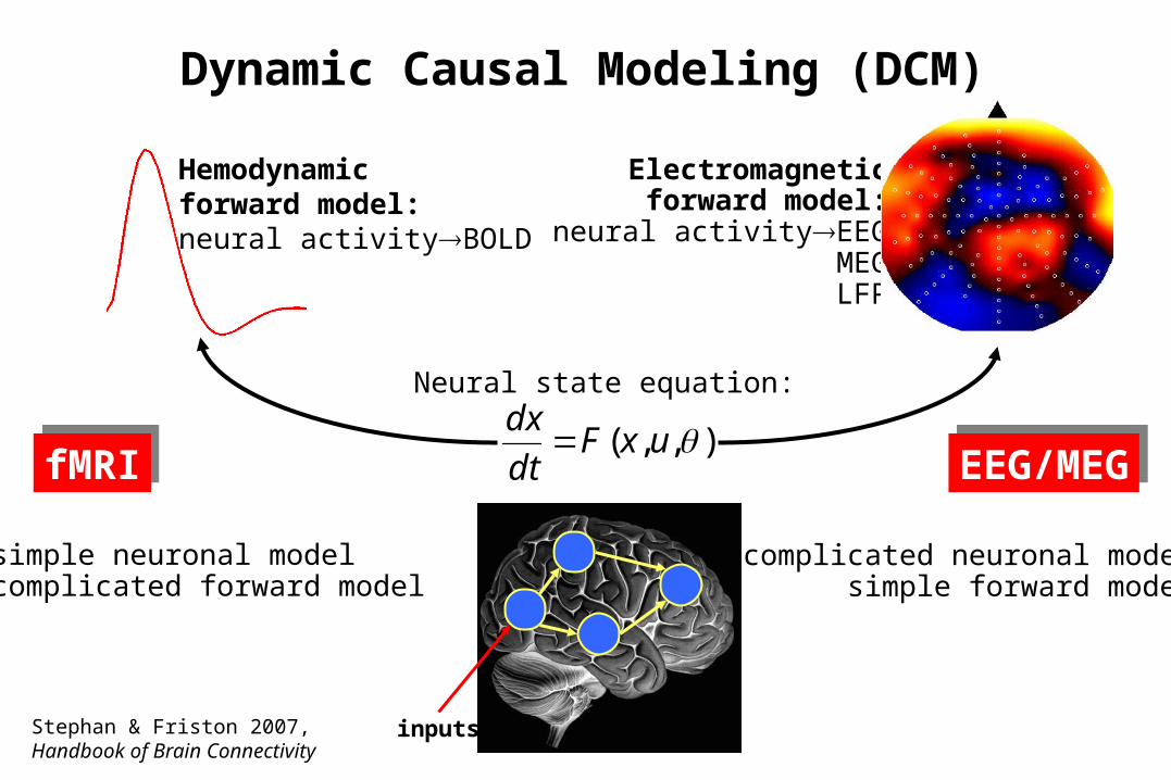
),,( uxFdt

dx

Neural state equation:

Electromagneticforward model:

neural activityEEGMEGLFP

Dynamic Causal Modeling (DCM)

simple neuronal modelcomplicated forward model

complicated neuronal modelsimple forward model

fMRIfMRI EEG/MEGEEG/MEG

inputs

Hemodynamicforward model:neural activityBOLD

Stephan & Friston 2007, Handbook of Brain Connectivity

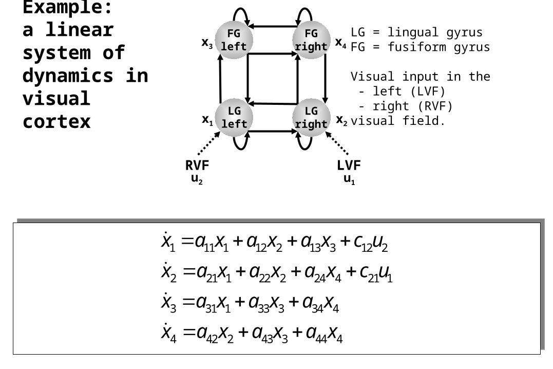
LGleft

LGright

RVF LVF

FGright

FGleft

LG = lingual gyrusFG = fusiform gyrus

Visual input in the - left (LVF) - right (RVF)visual field.x1 x2

x4x3

u2 u1

1 11 1 12 2 13 3 12 2

2 21 1 22 2 24 4 21 1

3 31 1 33 3 34 4

4 42 2 43 3 44 4

x a x a x a x c u

x a x a x a x c u

x a x a x a x

x a x a x a x

Example: a linear system of dynamics in visual cortex

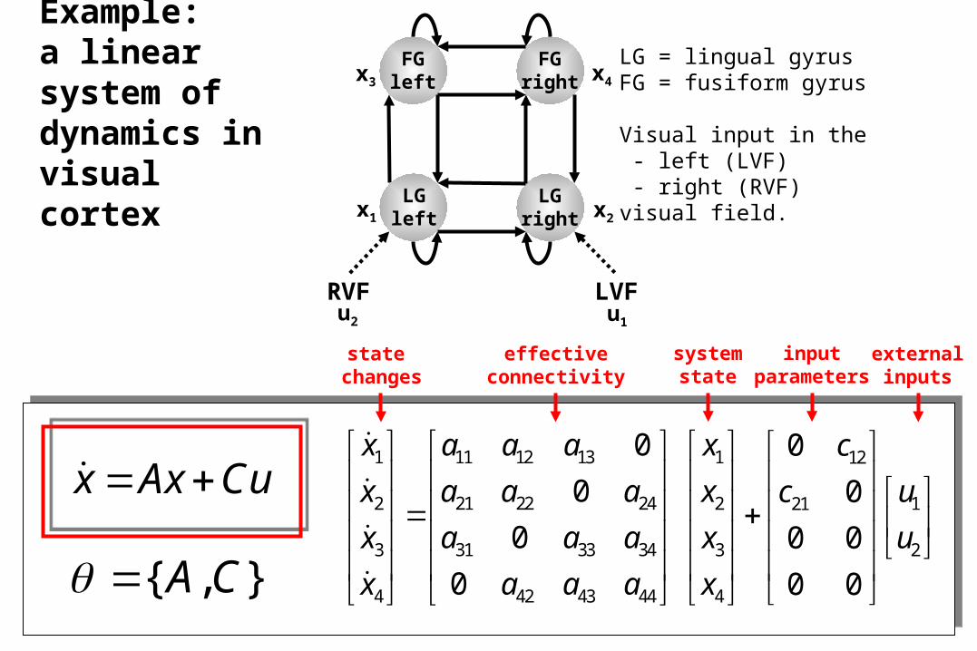
Example: a linear system of dynamics in visual cortex

LG = lingual gyrusFG = fusiform gyrus

Visual input in the - left (LVF) - right (RVF)visual field.

state changes

effectiveconnectivity

externalinputs

systemstate

inputparameters

11 12 131 1 12

21 22 242 2 121

31 33 343 3 2

42 43 444 4

0 0

0 0

0 0 0

0 0 0

a a ax x c

a a ax x uc

a a ax x u

a a ax x

x Ax Cu

},{ CA

LGleft

LGright

RVF LVF

FGright

FGleft

x1 x2

x4x3

u2 u1

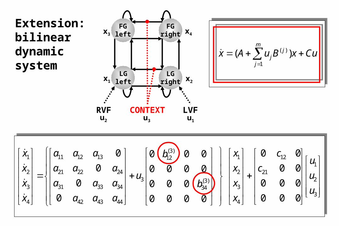
Extension: bilinear dynamic system

LGleft

LGright

RVF LVF

FGright

FGleft

x1 x2

x4x3

u2 u1

CONTEXTu3

( )

1

( )m

jj

j

x A u B x Cu

(3)11 12 131 1 1212

121 22 242 2 21

3 2(3)31 33 343 334

342 43 444 4

0 0 00 0 0

0 0 00 0 0 0

0 0 0 00 0 0

0 0 0 00 0 0 0

a a ax x cbu

a a ax x cu u

a a ax xbu

a a ax x

intrinsic connectivity

direct inputs

modulation ofconnectivity

Neural state equation CuxBuAx jj )( )(

u

xC

x

x

uB

x

xA

j

j

)(

hemodynamicmodelλ

x

y

integration

BOLDyyy

activityx1(t)

activityx2(t) activity

x3(t)

neuronalstates

t

drivinginput u1(t)

modulatoryinput u2(t)

t

Stephan & Friston (2007),Handbook of Brain Connectivity

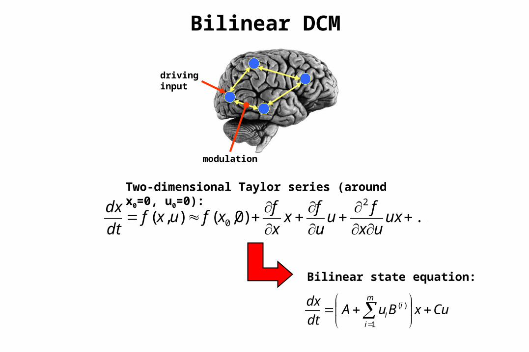
Bilinear DCM

CuxBuAdt

dx m

i

ii

1

)(

Bilinear state equation:

driving input

modulation

...)0,(),(2

0

uxux

fu

u

fx

x

fxfuxf

dt

dxTwo-dimensional Taylor series (around x0=0, u0=0):

-

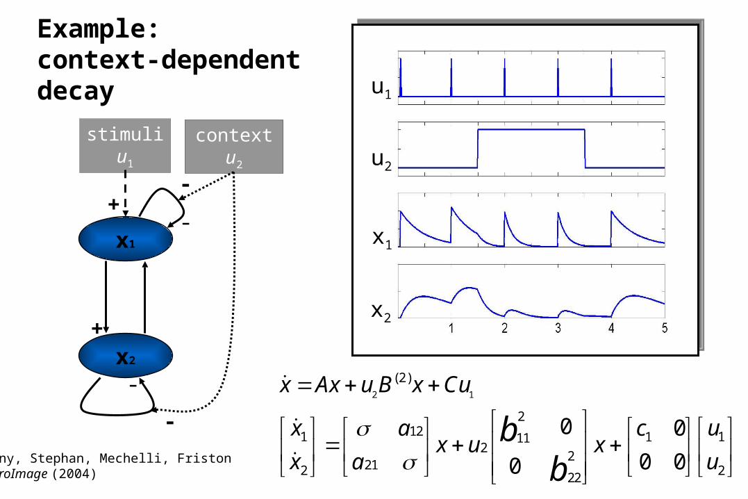
x2

stimuliu1

contextu2

x1

+

+

-

-

-+

u1

Z1

u2

Z2

2 1

(2)

2121 1111

22

212 222

0 0

0 00

x Ax u B x Cu

x ua cx u x

x uab

b

Example: context-dependent decay u1

u2

x2

x1

Penny, Stephan, Mechelli, Friston NeuroImage (2004)

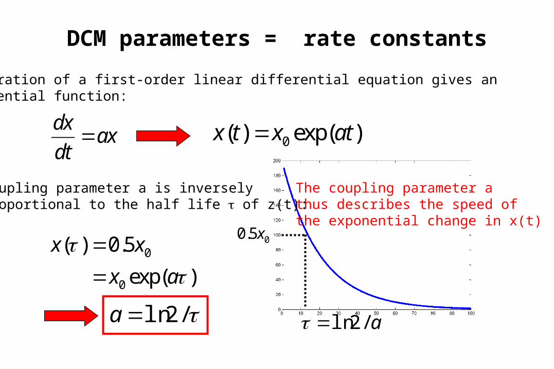
DCM parameters = rate constants

dxax

dt 0( ) exp( )x t x at

The coupling parameter a thus describes the speed ofthe exponential change in x(t)

0

0

( ) 0.5

exp( )

x x

x a

Integration of a first-order linear differential equation gives anexponential function:

/2lna

00.5x

a/2ln

Coupling parameter a is inverselyproportional to the half life of z(t):

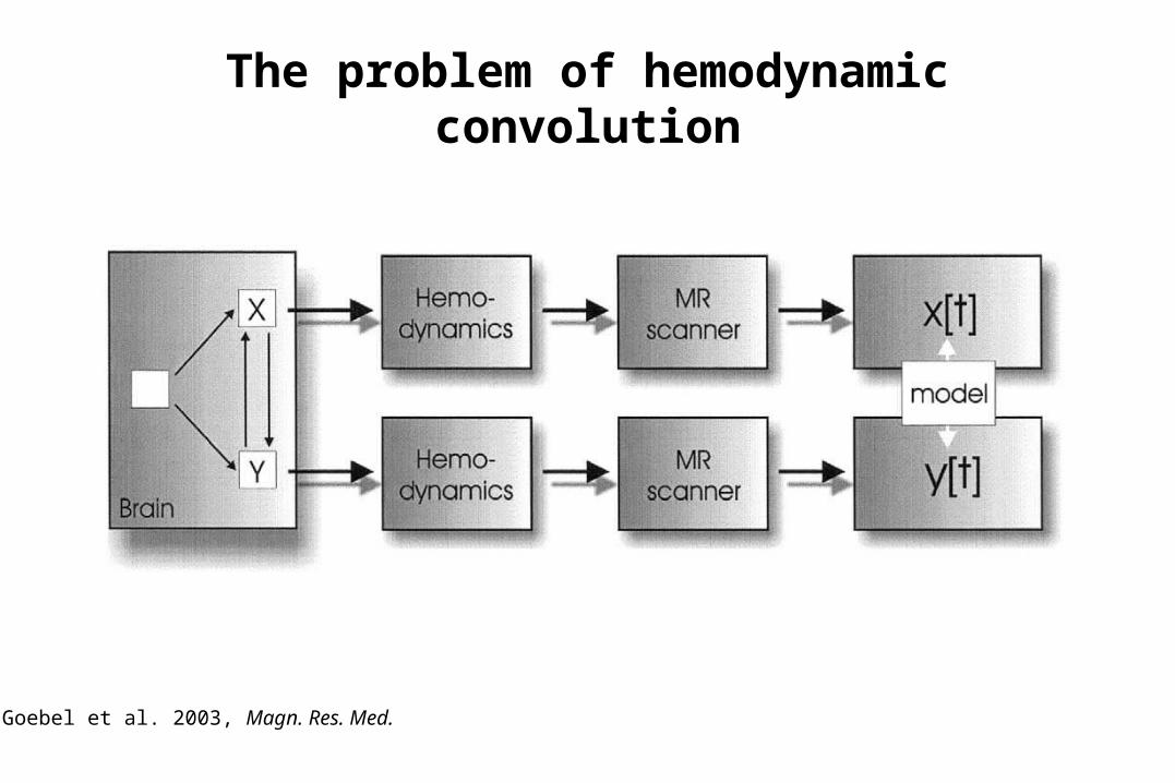
The problem of hemodynamic convolution

Goebel et al. 2003, Magn. Res. Med.

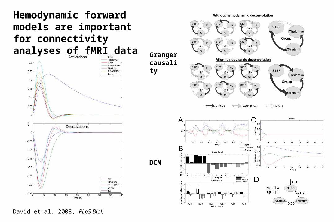
Hemodynamic forward models are important for connectivity analyses of fMRI data

David et al. 2008, PLoS Biol.

Granger causality

DCM

sf

tionflow induc

(rCBF)

s

v

stimulus functions

v

q q/vvEf,EEfqτ /α

dHbchanges in

100 )( /αvfvτ

volumechanges in

1

f

q

)1(

fγsxs

signalryvasodilato

u

s

CuxBuAdt

dx m

j

jj

1

)(

t

neural state equation

1

3.4

111),(

3

002

001

32100

k

TEErk

TEEk

vkv

qkqkV

S

Svq

hemodynamic state equationsf

Balloon model

BOLD signal change equation

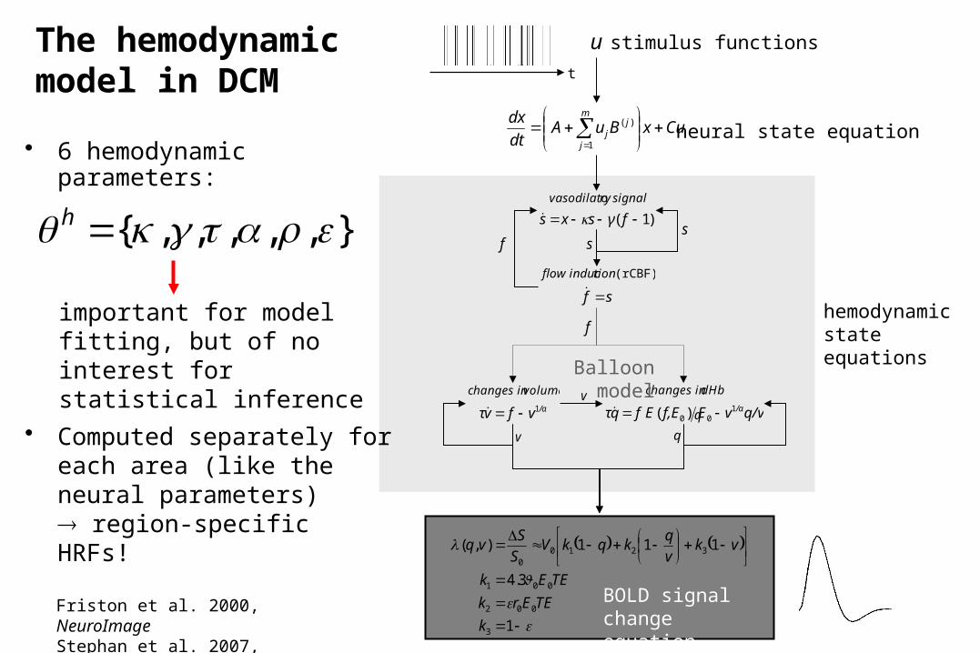
},,,,,{ h

important for model fitting, but of no interest for statistical inference

• 6 hemodynamic parameters:

• Computed separately for each area (like the neural parameters) region-specific HRFs!

The hemodynamic model in DCM

Friston et al. 2000, NeuroImageStephan et al. 2007, NeuroImage

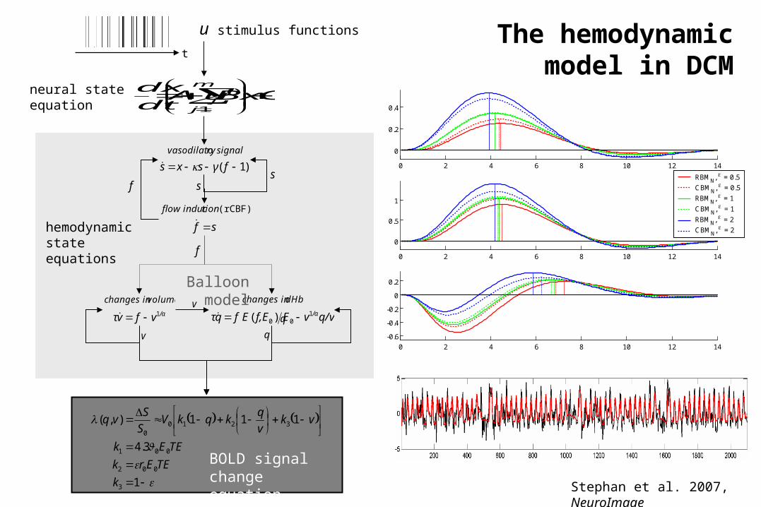
0 2 4 6 8 10 12 14

0

0.2

0.4

0 2 4 6 8 10 12 14

0

0.5

1

0 2 4 6 8 10 12 14

-0.6

-0.4

-0.2

0

0.2

RBMN

, = 0.5

CBMN

, = 0.5

RBMN

, = 1

CBMN

, = 1

RBMN

, = 2

CBMN

, = 2sf

tionflow induc

(rCBF)

s

v

stimulus functions

v

q q/vvEf,EEfqτ /α

dHbchanges in

100 )( /αvfvτ

volumechanges in

1

f

q

)1(

fγsxs

signalryvasodilato

u

s

CuxBuAdt

dx m

j

jj

1

)(

t

neural state equation

1

3.4

111),(

3

002

001

32100

k

TEErk

TEEk

vkv

qkqkV

S

Svq

hemodynamic state equations

f

Balloon model

BOLD signal change equation

The hemodynamic model in DCM

Stephan et al. 2007, NeuroImage

5 10 15 20 25 30 35 40

5

10

15

20

25

30

35

40

-1

-0.8

-0.6

-0.4

-0.2

0

0.2

0.4

0.6

0.8

1

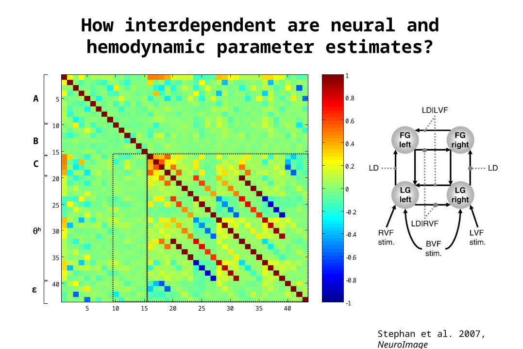
A

B

C

h

ε

How interdependent are neural and hemodynamic parameter estimates?

Stephan et al. 2007, NeuroImage

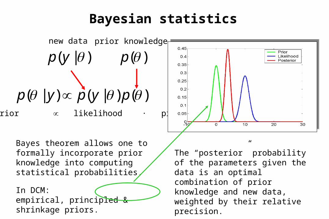
Bayesian statistics

)()|()|( pypyp posterior likelihood ∙ prior

)|( yp )(p

Bayes theorem allows one to formally incorporate prior knowledge into computing statistical probabilities.

In DCM: empirical, principled & shrinkage priors.

The “posterior” probability of the parameters given the data is an optimal combination of prior knowledge and new data, weighted by their relative precision.

new data prior knowledge

sf (rCBF)induction -flow

s

v

f

stimulus function u

modelled BOLD response

vq q/vvf,Efqτ /α1)(

dHbin changes

/αvfvτ 1

in volume changes

f

q

)1(

signalry vasodilatodependent -activity

fγszs

s

)(xy eXuhy ),(

observation model

hidden states{ , , , , }z x s f v q

state equation( , , )z F x u

parameters

},{

},...,{

},,,,{1

nh

mn

h

CBBA

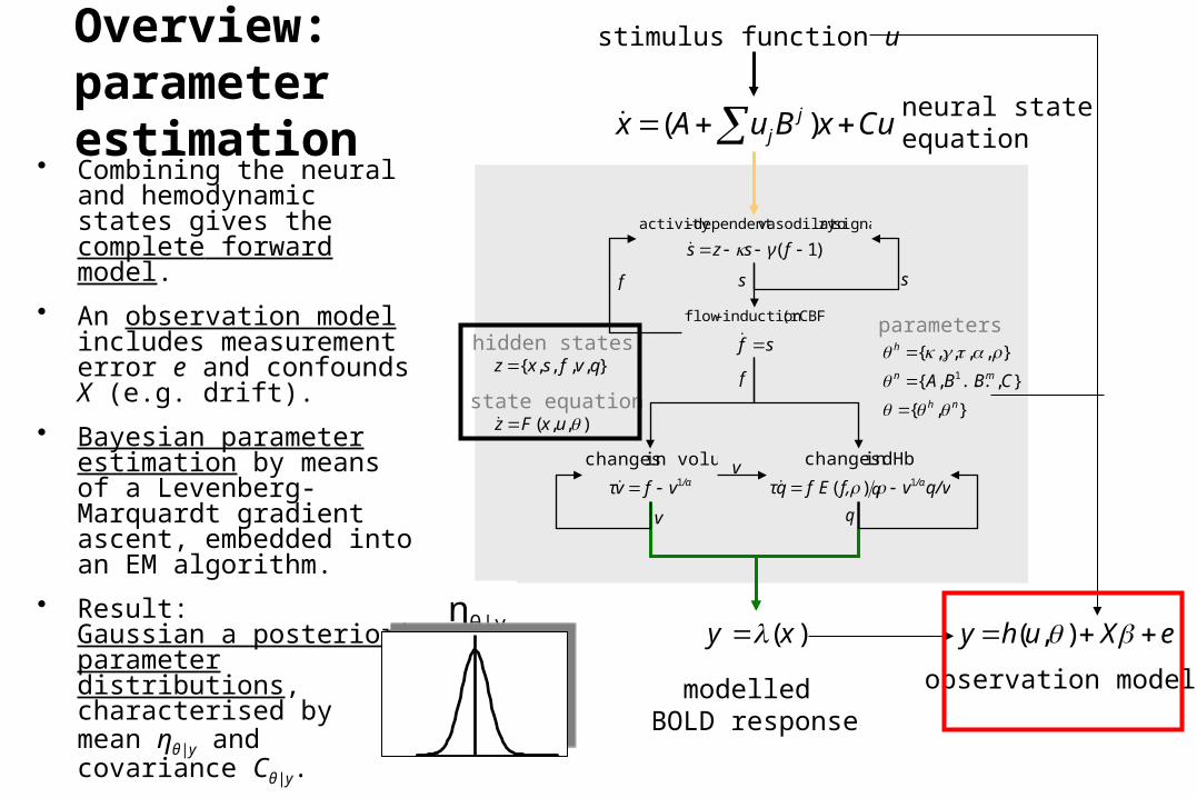
• Combining the neural and hemodynamic states gives the complete forward model.

• An observation model includes measurement error e and confounds X (e.g. drift).

• Bayesian parameter estimation by means of a Levenberg-Marquardt gradient ascent, embedded into an EM algorithm.

• Result:Gaussian a posteriori parameter distributions, characterised by mean ηθ|y and covariance Cθ|y.

Overview:parameter estimation

ηθ|y

neural stateequation( )j

jx A u B x Cu

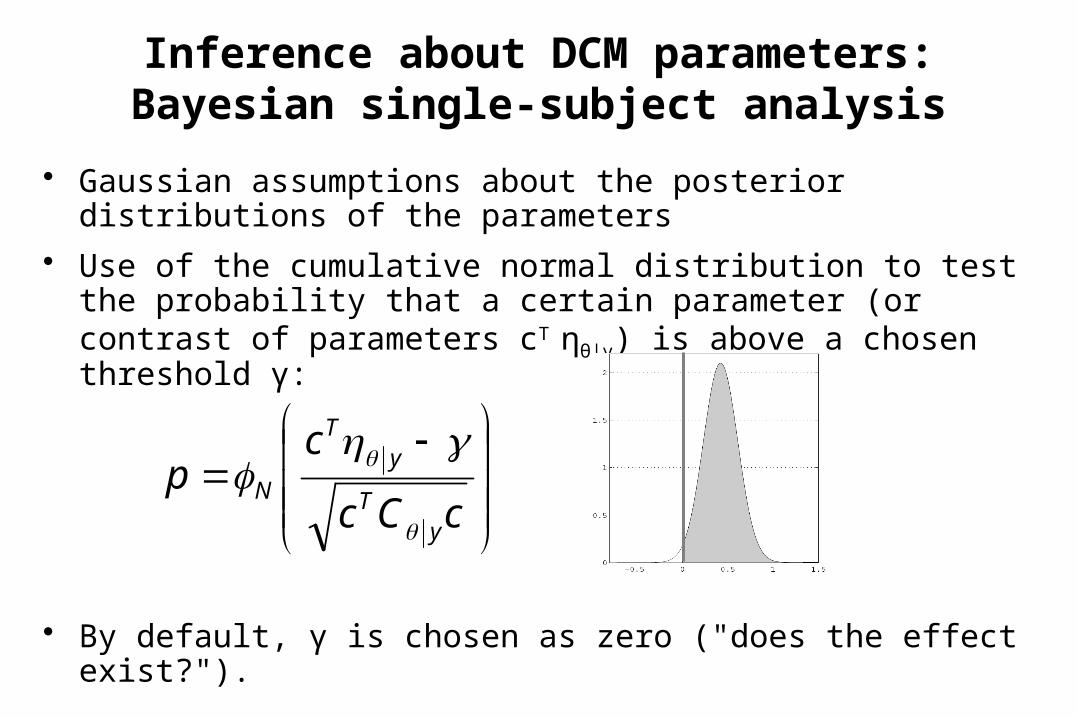
• Gaussian assumptions about the posterior distributions of the parameters

• Use of the cumulative normal distribution to test the probability that a certain parameter (or contrast of parameters cT ηθ|y) is above a chosen threshold γ:

• By default, γ is chosen as zero ("does the effect exist?").

Inference about DCM parameters:Bayesian single-subject analysis

cCc

cp

yT

yT

N

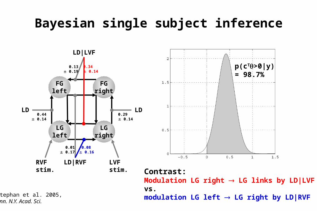
Bayesian single subject inference

LGleft

LGright

RVFstim.

LVFstim.

FGright

FGleft

LD|RVF

LD|LVF

LD LD

0.34 0.14

-0.08 0.16

0.13 0.19

0.01 0.17

0.44 0.14

0.29 0.14

Contrast:Modulation LG right LG links by LD|LVFvs.modulation LG left LG right by LD|RVF

p(cT>0|y) = 98.7%

Stephan et al. 2005, Ann. N.Y. Acad. Sci.

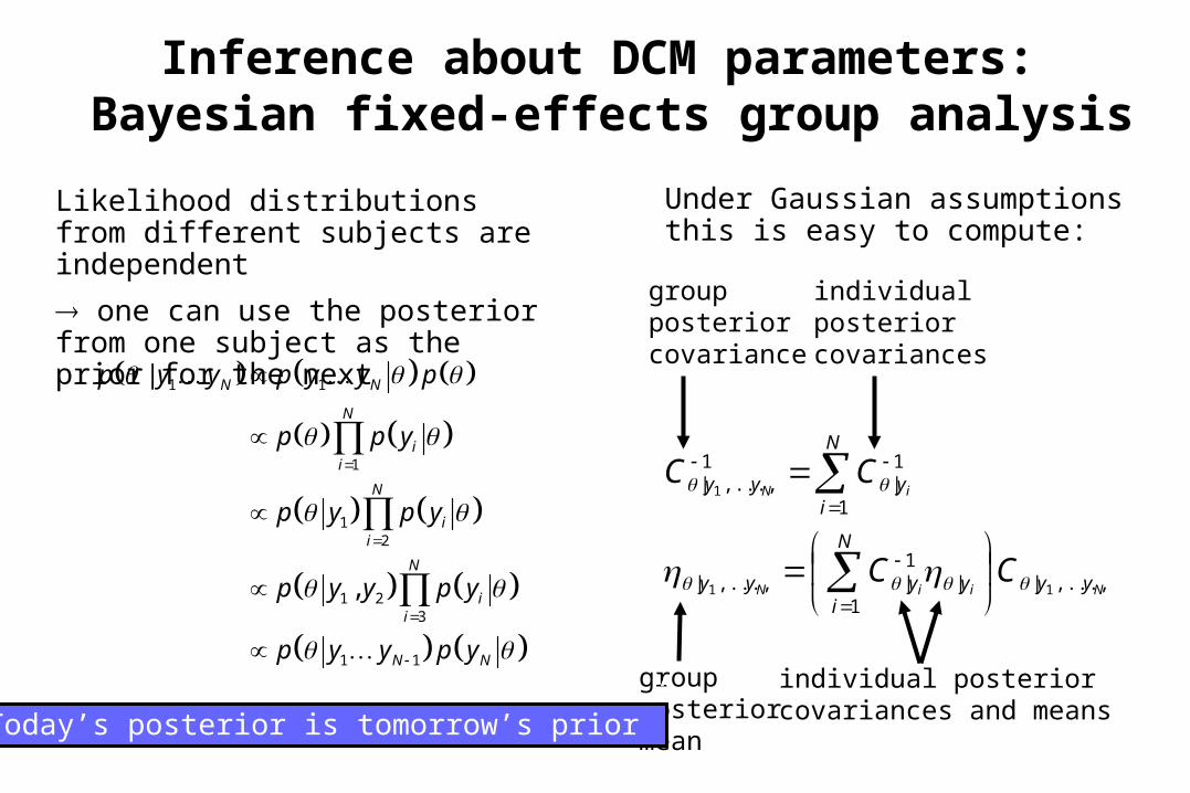
Likelihood distributions from different subjects are independent

one can use the posterior from one subject as the prior for the next

NiiN

iN

yy

N

iyyyy

N

iyyy

CC

CC

,...,|1

|1|,...,|

1

1|

1,...,|

11

1

Under Gaussian assumptions this is easy to compute:

groupposterior covariance

individualposterior covariances

groupposterior mean

individual posterior covariances and means“Today’s posterior is tomorrow’s prior”

Inference about DCM parameters: Bayesian fixed-effects group analysis

1 1

1

12

1 23

1 1

|

,

N N

N

ii

N

ii

N

ii

N N

p y y p y y p

p p y

p y p y

p y y p y

p y y p y

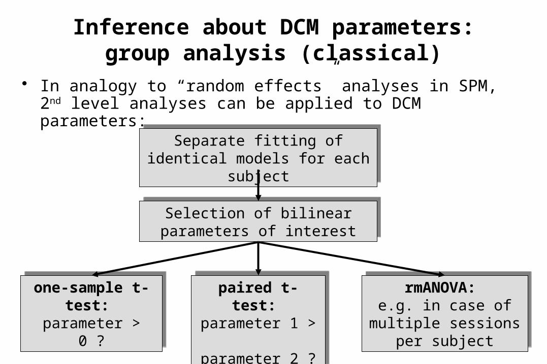
Inference about DCM parameters:group analysis (classical)

• In analogy to “random effects” analyses in SPM, 2nd level analyses can be applied to DCM parameters:

Separate fitting of identical models for each subject

Separate fitting of identical models for each subject

Selection of bilinear parameters of interestSelection of bilinear

parameters of interest

one-sample t-test:

parameter > 0 ?

one-sample t-test:

parameter > 0 ?

paired t-test: parameter 1 > parameter 2 ?

paired t-test: parameter 1 > parameter 2 ?

rmANOVA: e.g. in case of

multiple sessions per subject

rmANOVA: e.g. in case of

multiple sessions per subject

Overview





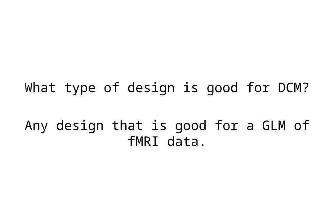
Any design that is good for a GLM of fMRI data.

What type of design is good for DCM?

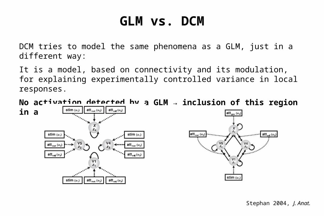
GLM vs. DCM

DCM tries to model the same phenomena as a GLM, just in a different way:

It is a model, based on connectivity and its modulation, for explaining experimentally controlled variance in local responses.

No activation detected by a GLM → inclusion of this region in a DCM is useless!

Stephan 2004, J. Anat.

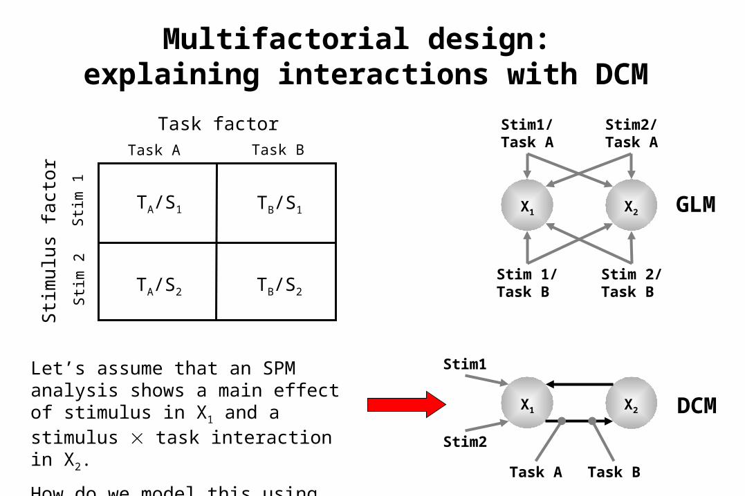
Multifactorial design: explaining interactions with DCM

Task factorTask A Task B

Sti

m 1

Sti

m 2

Sti

mu

lus

fact

or

TA/S1 TB/S1

TA/S2 TB/S2

X1 X2

Stim2/Task A

Stim1/Task A

Stim 1/Task B

Stim 2/Task B

GLM

X1 X2

Stim2

Stim1

Task A Task B

DCM

Let’s assume that an SPM analysis shows a main effect of stimulus in X1 and a stimulus task interaction in X2.

How do we model this using DCM?

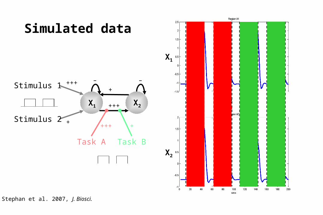
Stim 1Task A

Stim 2Task A

Stim 1Task B

Stim 2Task B

Simulated data

X1

X2

+++X1 X2

Stimulus 2

Stimulus 1

Task A Task B

+++++

++++

– –

Stephan et al. 2007, J. Biosci.

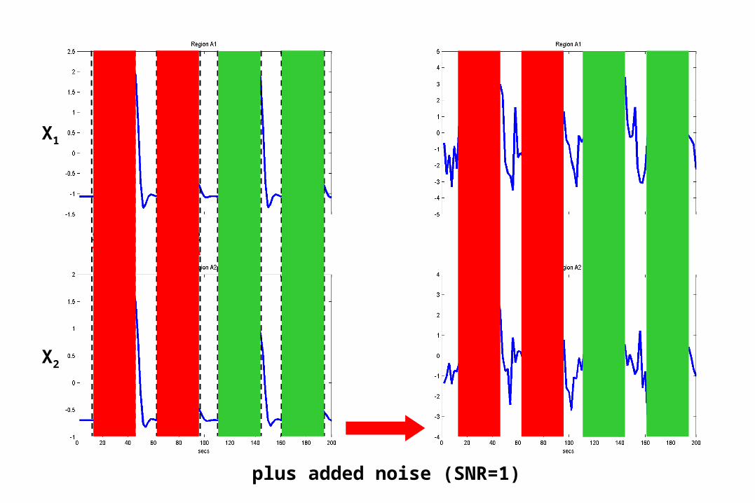
Stim 1Task A

Stim 2Task A

Stim 1Task B

Stim 2Task B

plus added noise (SNR=1)

X1

X2

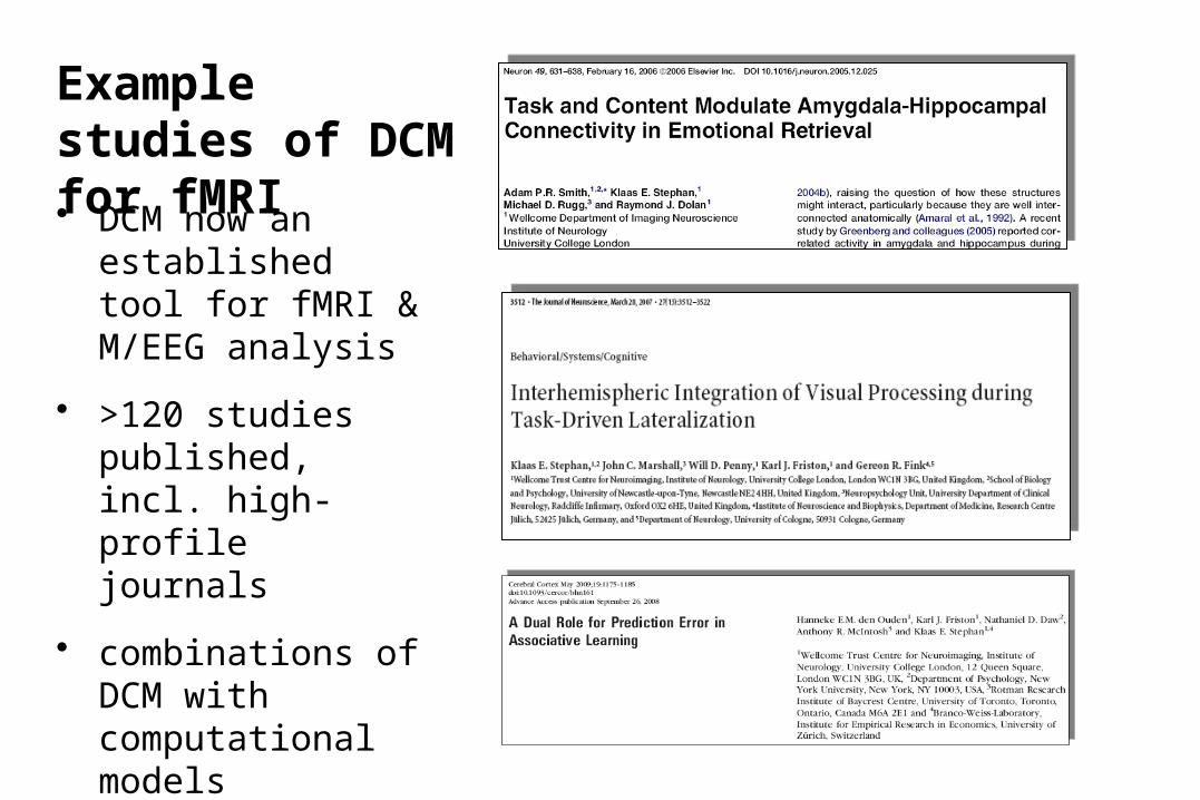
Example studies of DCM for fMRI• DCM now an

established tool for fMRI & M/EEG analysis

• >120 studies published, incl. high-profile journals

• combinations of DCM with computational models

Is the red letter left or right from the midline of the word?


analysis with SPM2


analysis with SPM2

Task-driven lateralisation

letter decisions > spatial decisions

time

•••

Does the word contain the letter A or not?

spatial decisions > letter decisions


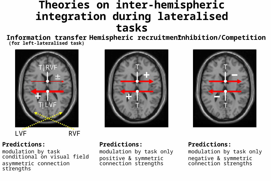
Theories on inter-hemispheric integration during lateralised

tasksInformation transfer

(for left-lateralised task)Inhibition/CompetitionHemispheric recruitment

LVF RVF

T

T

T

T+

−

−

T

T

+

+

Predictions:modulation by task conditional on visual fieldasymmetric connection strengths

Predictions:modulation by task onlynegative & symmetricconnection strengths

Predictions:modulation by task onlypositive & symmetricconnection strengths

|LVF

|RVF

LGleft

LGright

FGright

FGleft

RVF LVF

B

A

Bcond

Bind

LD

VF

VF LD Bind Bcond

intra

inter16 models

LGleft

LGright

FGright

FGleft

LD

RVF

LVF

LGleft

LGright

RVFstim.

LVFstim.

FGright

FGleft

LD

LD,RVF

LD|RVF

LD

LD,LVF

LD|LVF

VF

LD

Bind

Bcond

LD

RVF

LVF

LD|RVF

LD|LVF

VF LD Bind BcondD

C

LGleft

LGright

RVFstim.

LVFstim.

FGright

FGleft

LD|RVF

LD|LVF

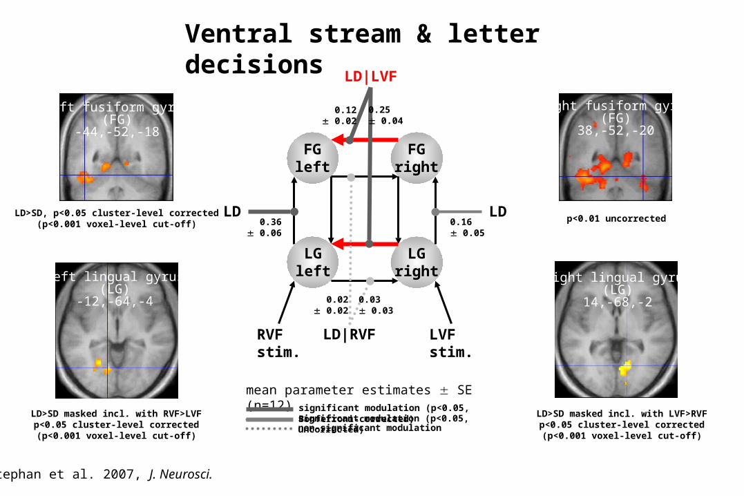
LD LD

0.25 0.04

0.03 0.03

0.12 0.02

0.02 0.02

0.36 0.06

0.16 0.05

Left lingual gyrus(LG)

-12,-64,-4

Left fusiform gyrus(FG)

-44,-52,-18

Right fusiform gyrus(FG)

38,-52,-20

Right lingual gyrus(LG)

14,-68,-2

mean parameter estimates SE (n=12)

significant modulation (p<0.05, uncorrected)non-significant modulation

significant modulation (p<0.05, Bonferroni-corrected)LD>SD masked incl. with RVF>LVF

p<0.05 cluster-level corrected(p<0.001 voxel-level cut-off)

LD>SD, p<0.05 cluster-level corrected(p<0.001 voxel-level cut-off)

p<0.01 uncorrected

LD>SD masked incl. with LVF>RVFp<0.05 cluster-level corrected(p<0.001 voxel-level cut-off)

Ventral stream & letter decisions

Stephan et al. 2007, J. Neurosci.

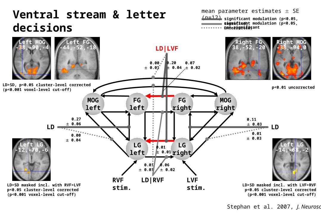
MOGleft

LGleft

LGright

RVFstim.

LVFstim.

FGright

FGleft

LD|RVF

LD|LVF

LD LD

0.20 0.04

0.06 0.02

0.00 0.01

0.01 0.01

0.27 0.06

0.11 0.03

MOGright

0.00 0.04

0.01 0.03

0.07 0.02

0.01 0.01

Ventral stream & letter decisions

LD>SD, p<0.05 cluster-level corrected(p<0.001 voxel-level cut-off)

Left MOG-38,-90,-4

mean parameter estimates SE (n=12)

significant modulation (p<0.05, uncorrected)non-significant

significant modulation (p<0.05, corrected)

Left FG-44,-52,-18

Right MOG-38,-94,0

p<0.01 uncorrected

Left LG-12,-70,-6

Left LG-14,-68,-2

LD>SD masked incl. with RVF>LVFp<0.05 cluster-level corrected(p<0.001 voxel-level cut-off)

LD>SD masked incl. with LVF>RVFp<0.05 cluster-level corrected

(p<0.001 voxel-level cut-off)

Right FG38,-52,-20


-0.2

-0.1

0.0

0.1

0.2

0.3

0.4

0.5

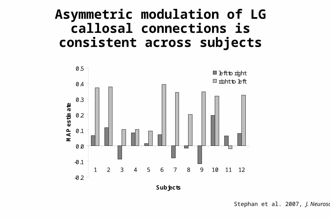
1 2 3 4 5 6 7 8 9 10 11 12

Subjects

MA

P e

sti

ma

teleft to right

right to left

Asymmetric modulation of LG callosal connections is

consistent across subjects


Fixation cross

Auditory

Auditory VisualFixation cross

Time (ms)

0 200

400

600

800

1000

1200

2000 ± 500

or

Visual

“Distractor”Target

“Distractor”

Target

1400

Incidental learning of audio-visual associations

Hypothesis: Incidental learning of this relation is reflected by prediction-error dependent changes in connectivity between auditory and visual areas.

80%

80%

den Ouden et al. 2009, Cereb. Cortex

Incidental learning of audio-visual associations

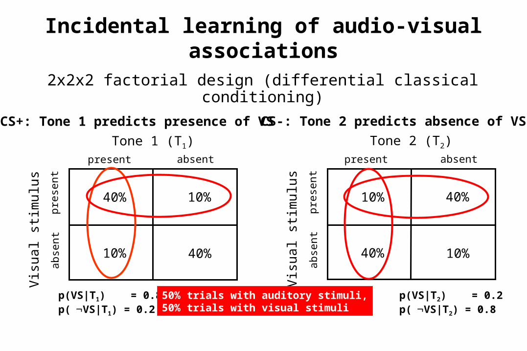
2x2x2 factorial design (differential classical conditioning)

Tone 1 (T1)present absent

pre

sent

abse

nt

Vis

ual st

imu

lus

40%

10%

10%

40%

Tone 2 (T2)present absent

pre

sent

abse

nt

Vis

ual st

imu

lus

10%

40%

40%

10%

CS+: Tone 1 predicts presence of VSCS-: Tone 2 predicts absence of VS

p(VS|T1) = 0.8p(VS|T1) = 0.2

p(VS|T2) = 0.2p(VS|T2) = 0.8

50% trials with auditory stimuli,50% trials with visual stimuli

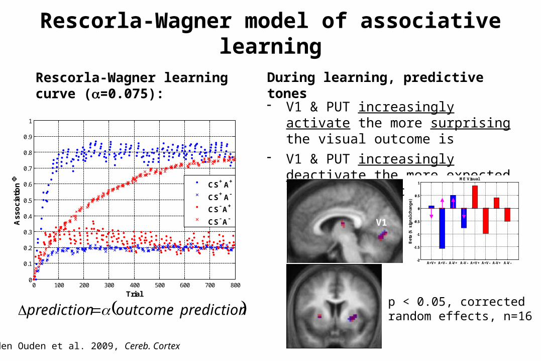
Rescorla-Wagner model of associative learning

p < 0.05, correctedrandom effects, n=16

- V1 & PUT increasingly activate the more surprising the visual outcome is

- V1 & PUT increasingly deactivate the more expected the visual outcome is

Rescorla-Wagner learningcurve (=0.075):

predictionoutcomeprediction

During learning, predictive tones

V1PUT

0 100 200 300 400 500 600 700 8000

0.1

0.2

0.3

0.4

0.5

0.6

0.7

0.8

0.9

1

Trial

As

so

cia

tio

n

CS+ A+

CS+ A-

CS- A+

CS- A-

A+V+ A+V- A-V+ A-V- A+V+ A+V- A-V+ A-V--2

-1.5

-1

-0.5

0

0.5

1

Bet

a (%

sig

nal

ch

ang

e)

ME Visual


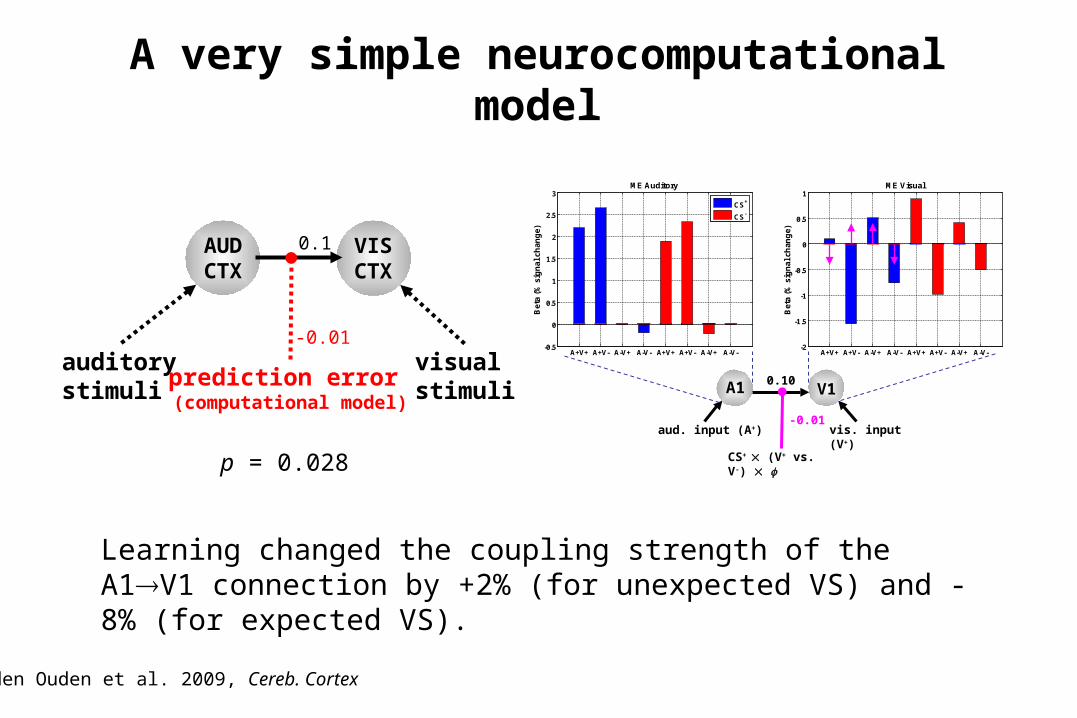
AUDCTX

VISCTX

auditorystimuli

visualstimuliprediction error

(computational model)

A very simple neurocomputational model

Learning changed the coupling strength of the A1V1 connection by +2% (for unexpected VS) and -8% (for expected VS).

0.1

-0.01

A1 V1

aud. input (A+) vis. input (V+)

CS+ (V+ vs. V-)

A+V+ A+V- A-V+ A-V- A+V+ A+V- A-V+ A-V--2

-1.5

-1

-0.5

0

0.5

1

Bet

a (%

sig

nal

ch

ang

e)

ME Visual

A+V+ A+V- A-V+ A-V- A+V+ A+V- A-V+ A-V--0.5

0

0.5

1

1.5

2

2.5

3

Bet

a (%

sig

nal

ch

ang

e)

ME Auditory

CS+

CS-

0.10

-0.01

p = 0.028


Thank you

Documents

Models of effective connectivity & Dynamic Causal Modelling (DCM) Klaas Enno Stephan Laboratory for Social & Neural Systems Research Institute for Empirical