Models for Tropopause Height and

Radiative-Convective Equilibrium

Shineng Hu

August 16, 2015

1 Introduction

Radiative-convective equilibrium (RCE) is the equilibrium state that a convective systemreaches, where convective heating compensates radiative cooling. RCE has often been usedto represent the planetary atmosphere on a global scale, and it is also useful for studyingthe tropical climates since tropical atmosphere is always believed to reside in a near RCEstate.

There is a hierarchy of numerical models that have been developed to study the RCEsystem, ranging from radiative-convective models (RCMs) with parameterized convection tocloud resolving models (CRMs) with explicit convective processes. Those numerical modelshave led us to a much deeper understanding of the radiative-convective system, but thebasic physics of RCE is still far from fully understood.

One important reason is that, although the RCE concept is already simplified fromreality, the full RCE system (or model) is still too complicated at least in two aspects.First, radiative and convective processes are highly coupled and nonlinear. For example,convection transports water vapor from the boundary layer to the free troposphere, andit effectively influences the absorbed longwave radiation in the atmosphere, which in turnaffects the local buoyancy (temperature) and thus convection. Second, current RCMs orCRMs are usually divided into tens of vertical layers. The exchange of mass and energybetween different layers makes the system very difficult to diagnose.

To better understand the RCE system, one can try to simplify either aspect above, andthis is one of the motivations of this study. Accordingly, the main goal of this study istwofold. The first part will stick with multiple layers, but try to reduce the coupling of thesystem by specifying some variables like lapse rate and optical depth. One main goal ofthis part is to understand the structure of earth’s tropopause by taking advantage of thesimplifications we made here. The second part will try to develop a maximally simplifiedRCE model with an interactive hydrological cycle to better understand the basic physics ofRCE itself. This model contains two layers in troposphere, but the convective and radiativeprocesses are still highly coupled. More details will be discussed below.

240

2 The height of tropopause

2.1 Background

Tropopause is usually referred to as the boundary between the troposphere and the strato-sphere, even though it has various definitions based on the spatial structures of temperature,potential vorticity, and chemical concentrations. Understanding the height of tropopause isimportant to studying the column total ozone [1] and also the mass exchange between thetroposphere and the stratosphere [2].

Despite its importance, many problems related to the observed features of the tropopauseremain unsolved. From observations, the height of tropopause is higher in the tropics (16km)and lower in the polar regions (8km), and this transition sharply occurs in the mid-latitudes(Fig. 1a). What shapes this particular structure? Also, tropical tropopause, compared withthe one in extratropics, is not only higher, but also colder and sharper (Fig. 1b). What canexplain those three features simultaneously?

(a) (b)

Latitude (°N)Latitude (°N)

Hei

ght (

m)

Figure 1: (a) Zonal-mean tropopause height as a function of latitude (solid). Figure adoptedfrom [3]. (b) Zonal mean temperature profiles in different regions. Note the contrast betweentropics (blue dash-dotted) and extratropics (green dashed). Figure adopted from [4].

To that end, we will use a extremely simplified tropopause model, and see whether thisone-dimensional (1-D) model can reproduce the observed structure of tropopause. Onething noteworthy is that there will be no explicit dynamics in this model, although lateraltransport and mid-latitude eddies are shown to be important in shaping the tropopausestructure. Our following results will show that the observed features of tropopause can besurprisingly well captured by this simple 1-D model.

2.2 Numerical model

Let’s start with a two-stream grey atmosphere, which is commonly used in early relatedstudies [5, 6], and write the radiation transfer equation for longwave radiation as,

∂D

∂τ= B −D, ∂U

∂τ= U −B, (2.1)

241

200 220 240 260 280 300 320 340 360

Temperature (K)0

2

4

6

8

10

12

14

Heig

ht

(km

)

RE

RCE

Figure 2: Temperature profiles for radiative equilibrium (green) and radiative-convectiveequilibrium (black).

whereD and U are downward and upward longwave radiation, B = σT 4 is Stefan-Boltzmannlaw, and τ is optical depth increasing downward. Then we can quickly rewrite Eq. (2.1) as

∂I

∂τ= J − 2B,

∂J

∂τ= I (2.2)

usingI = U −D, J = U +D. (2.3)

Consider a radiative equilibrium (RE) state and assume that no shortwave radiation isabsorbed by the atmosphere, then the convergence of net longwave radiation should vanish,which can be expressed as,

∂I

∂τ= 0. (2.4)

Furthermore, by using the boundary condition at the top of the atmosphere,

τ = 0 : U = Ut = σT 4e , D = 0 (2.5)

we arrive at the solutions for radiative equilibrium,

D(τ), U(τ), B(τ) =

(τ

2,τ + 2

2,τ + 1

2

)Ut. (2.6)

The temperature profile from this solution is shown as the green line in Fig. 2

242

Let’s look at several features of RE solutions. When τ is very small, B/U is one half,and it physically means that near the top of the atmosphere, half of upward longwaveradiation is coming from remote radiative transfer. Note that, until now, we have notused any boundary condition at the surface. So this observation will be valid for any caseswith any lower boundary conditions, as long as the upper atmosphere is in the radiativeequilibrium state; it will be used in the following analysis when we are deriving the analyticalapproximation of RCE solutions. Now consider at the surface, the difference between U andB is always non-zero. It indicates that there is always a temperature jump between groundtemperature and near-surface air temperature in RE solutions, and this temperature jumpis actually nontrivial, around 10K. Another main feature is that the lapse rate near thesurface is so high that convection can occur, which will result in a new equilibrium statecalled radiative-convective equilibrium (RCE) state.

Within this new equilibrium state, the system is in RE in the stratosphere, given by thesolutions above, while in RCE in the troposphere with a uniform lapse rate. Mathematically,the temperature profile can be expressed as,

T (z) =

{Tre, z ≥ HT ,

TT + Γ(HT − z), HT ≥ z ≥ 0,(2.7)

where HT is the tropopause height, and TT is the tropopause temperature. The two verticalcoordinates (τ and z) can be related by the formulation below,

τ(z) = τs [fH2Oexp(−z/Ha) + (1− fH2O)exp(−z/Hs)] (2.8)

where τs is surface optical depth, fH2O is a linear parameter controlling the contributionof water vapor to optical depth compared with carbon dioxide, Ha is the scale height ofwater vapor (typically 2km), and Hs is the scale height of carbon dioxide (typically 8km).Additionally, we should add one more boundary condition at the surface,

τ = τs : U = B = σT 4s . (2.9)

We can solve this set of equations numerically by integrating Eq. (2.1) from the top ofthe atmosphere to the surface given a certain HT , and iterate the calculation to match bothboundary conditions. The temperature profile associated with the RCE solutions is shownas the black curve in Fig. 2.

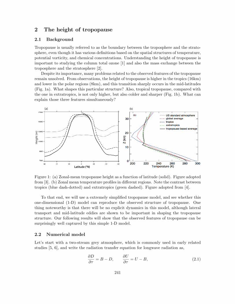
Note that the RCE solution above is a function of emission temperature Te, surfaceoptical depth τs, and tropospheric lapse rate Γ. The sensitivity of tropopause height tothose three parameters are presented in Fig. 3. Tropopause height significantly increaseswhen surface optical depth increases or tropospheric lapse rate decreases; tropopause heightincreases with outgoing longwave radiation but its impact is not as strong as the other twoparameters.

2.3 Analytical approximation

To better understand the phase diagrams in Fig. 3, it is helpful to derive an analyticalexpression for tropopause height. However, finding the exact analytical solution is very dif-ficult due to the multiple-layer model set-up and the nonlinearity of the system. Therefore,

243

(a) (b)

Figure 3: Tropopause height as a function of surface optical depth and (a) troposphericlapse rate and (b) outgoing longwave radiation. Note that the parameter ranges are chosenas typical ranges of earth’s atmosphere.

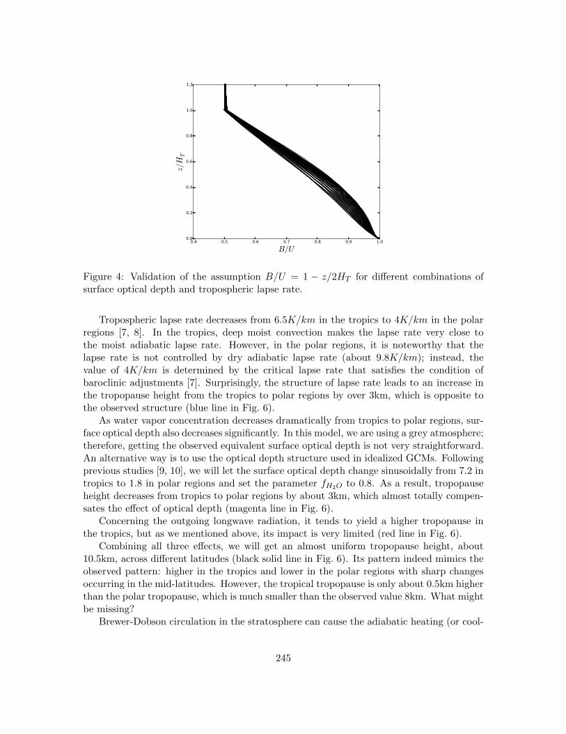
we make the following assumptions. First, temperatures above the tropopause are uniformand equal to 2−1/4Te, which is obtained from Eq. (2.6) by simply setting τ to be zero. Sec-ond, as mentioned before, the lapse rate is held uniform throughout the whole tropospherebelow HT . Third, the contribution to optical depth all comes from water vapor, that is,fH2O is set to 1. Fourth, B/U linearly increases from 1/2 (radiative equilibrium when τis zero) at the tropopause to 1 (lower boundary condition) at the surface, which can beexpressed as B/U = 1 − z/2HT , and this assumption is fairly good for a wide range ofsurface optical depth and tropospheric lapse rate as shown in Fig. 4.

With those assumptions, we can eventually derive an analytical approximation for theheight of tropopause as follows,

HT =1

16Γ

(CTT +

√C2T 2

T + 32ΓτsHaTT

), (2.10)

where C = ln4 ≈ 1.38. This expression agrees quite well with the sensitivity resultspresented in Fig. 3.

2.4 What shapes the observed tropopause structure from an RCE per-spective? The role of Brewer-Dobson circulation

One question we can ask is could we reproduce the observed tropopause structure usingthis 1-D RCE model? To this end, we should first get the observed latitude dependence oflapse rate, optical depth, and outgoing longwave radiation, and then plug them into thissimple model. We will go through those three parameters as inputs one by one, and onlythe zonal-mean annual-mean results will be discussed.

244

0.4 0.5 0.6 0.7 0.8 0.9 1.0

B/U

0.0

0.2

0.4

0.6

0.8

1.0

1.2

z/HT

Figure 4: Validation of the assumption B/U = 1 − z/2HT for different combinations ofsurface optical depth and tropospheric lapse rate.

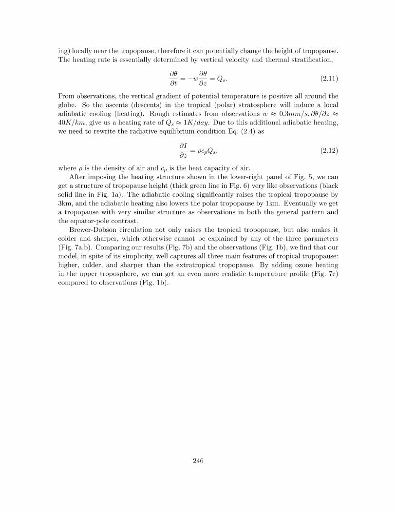
Tropospheric lapse rate decreases from 6.5K/km in the tropics to 4K/km in the polarregions [7, 8]. In the tropics, deep moist convection makes the lapse rate very close tothe moist adiabatic lapse rate. However, in the polar regions, it is noteworthy that thelapse rate is not controlled by dry adiabatic lapse rate (about 9.8K/km); instead, thevalue of 4K/km is determined by the critical lapse rate that satisfies the condition ofbaroclinic adjustments [7]. Surprisingly, the structure of lapse rate leads to an increase inthe tropopause height from the tropics to polar regions by over 3km, which is opposite tothe observed structure (blue line in Fig. 6).

As water vapor concentration decreases dramatically from tropics to polar regions, sur-face optical depth also decreases significantly. In this model, we are using a grey atmosphere;therefore, getting the observed equivalent surface optical depth is not very straightforward.An alternative way is to use the optical depth structure used in idealized GCMs. Followingprevious studies [9, 10], we will let the surface optical depth change sinusoidally from 7.2 intropics to 1.8 in polar regions and set the parameter fH2O to 0.8. As a result, tropopauseheight decreases from tropics to polar regions by about 3km, which almost totally compen-sates the effect of optical depth (magenta line in Fig. 6).

Concerning the outgoing longwave radiation, it tends to yield a higher tropopause inthe tropics, but as we mentioned above, its impact is very limited (red line in Fig. 6).

Combining all three effects, we will get an almost uniform tropopause height, about10.5km, across different latitudes (black solid line in Fig. 6). Its pattern indeed mimics theobserved pattern: higher in the tropics and lower in the polar regions with sharp changesoccurring in the mid-latitudes. However, the tropical tropopause is only about 0.5km higherthan the polar tropopause, which is much smaller than the observed value 8km. What mightbe missing?

Brewer-Dobson circulation in the stratosphere can cause the adiabatic heating (or cool-

245

ing) locally near the tropopause, therefore it can potentially change the height of tropopause.The heating rate is essentially determined by vertical velocity and thermal stratification,

∂θ

∂t= −w∂θ

∂z= Qs. (2.11)

From observations, the vertical gradient of potential temperature is positive all around theglobe. So the ascents (descents) in the tropical (polar) stratosphere will induce a localadiabatic cooling (heating). Rough estimates from observations w ≈ 0.3mm/s, ∂θ/∂z ≈40K/km, give us a heating rate of Qs ≈ 1K/day. Due to this additional adiabatic heating,we need to rewrite the radiative equilibrium condition Eq. (2.4) as

∂I

∂z= ρcpQs, (2.12)

where ρ is the density of air and cp is the heat capacity of air.After imposing the heating structure shown in the lower-right panel of Fig. 5, we can

get a structure of tropopause height (thick green line in Fig. 6) very like observations (blacksolid line in Fig. 1a). The adiabatic cooling significantly raises the tropical tropopause by3km, and the adiabatic heating also lowers the polar tropopause by 1km. Eventually we geta tropopause with very similar structure as observations in both the general pattern andthe equator-pole contrast.

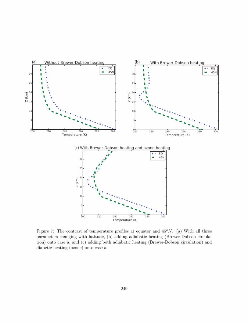
Brewer-Dobson circulation not only raises the tropical tropopause, but also makes itcolder and sharper, which otherwise cannot be explained by any of the three parameters(Fig. 7a,b). Comparing our results (Fig. 7b) and the observations (Fig. 1b), we find that ourmodel, in spite of its simplicity, well captures all three main features of tropical tropopause:higher, colder, and sharper than the extratropical tropopause. By adding ozone heatingin the upper troposphere, we can get an even more realistic temperature profile (Fig. 7c)compared to observations (Fig. 1b).

246

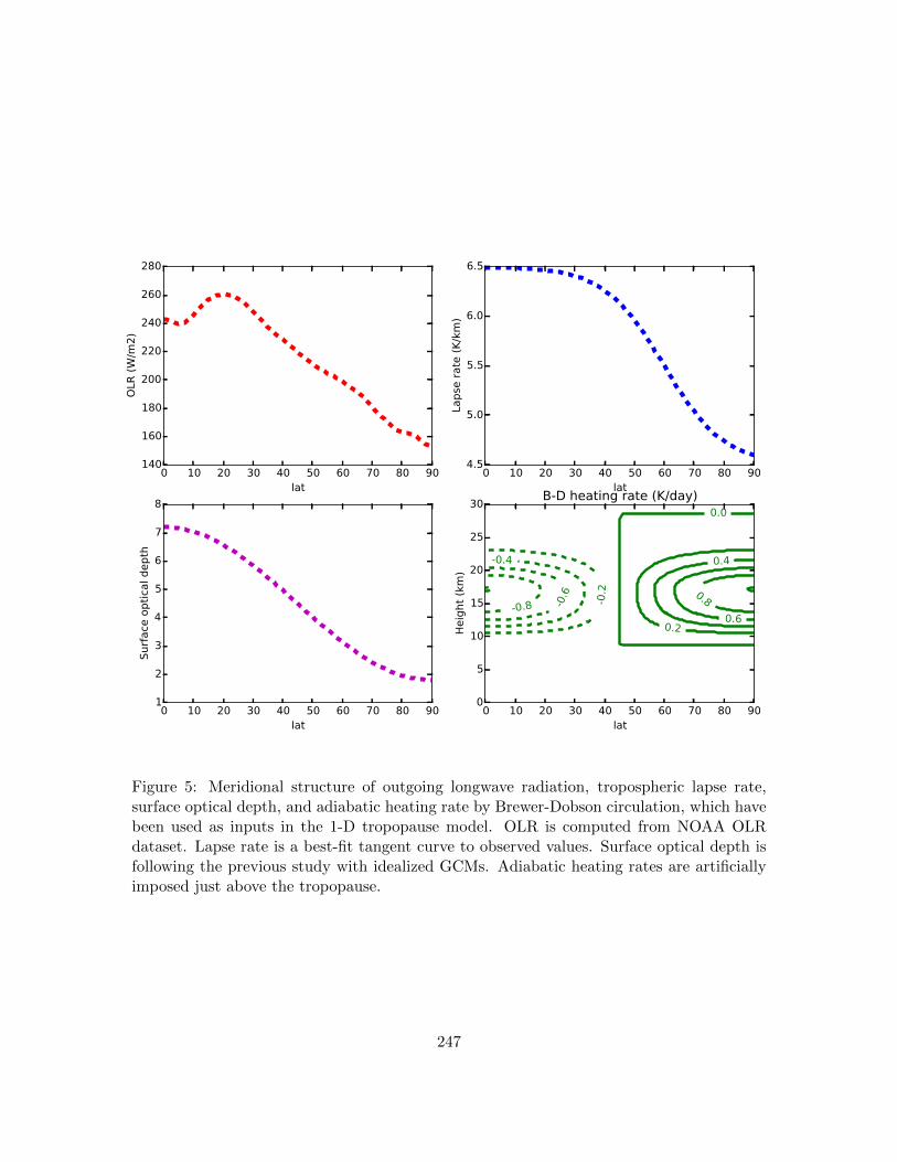
Figure 5: Meridional structure of outgoing longwave radiation, tropospheric lapse rate,surface optical depth, and adiabatic heating rate by Brewer-Dobson circulation, which havebeen used as inputs in the 1-D tropopause model. OLR is computed from NOAA OLRdataset. Lapse rate is a best-fit tangent curve to observed values. Surface optical depth isfollowing the previous study with idealized GCMs. Adiabatic heating rates are artificiallyimposed just above the tropopause.

247

0 10 20 30 40 50 60 70 80 90

lat

8

9

10

11

12

13

14

Heig

ht

of

tropopause

(km

)

Constant(a) Lapse rate(b) Optical depth(c) OLR(a)+(b)+(c)(a)+(b)+(c)+BD

Figure 6: Meridional structure of tropopause height from the numerical solutions of 1-Dtropopause model. The black dashed line is with all parameters constant. Three thin colorlines are with only lapse rate (blue), optical depth (magenta), or OLR (red) changing withlatitude. The thick black solid line is with all three parameters changing with latitude.The thick green solid line is with all three parameters changing with latitude and also animposed adiabatic heating by Brewer-Dobson circulation.

248

(a) (b)

(c)

Figure 7: The contrast of temperature profiles at equator and 45oN . (a) With all threeparameters changing with latitude, (b) adding adiabatic heating (Brewer-Dobson circula-tion) onto case a, and (c) adding both adiabatic heating (Brewer-Dobson circulation) anddiabetic heating (ozone) onto case a.

249

3 A two-layer RCE model

3.1 Background

In the tropopause model we just talked about, radiation and convection are two separateprocesses. Radiation accounts for the energy balance of the system, while convection acts toset the tropospheric lapse rate. In reality, the two processes are highly coupled. There arequite a few RCE studies with highly coupled models, such as radiative-convective models(RCMs) and cloud resolving models (CRMs), but they are too complicated to help usunderstand the principle physics of RCE states. For example, how does relative humiditychange with climates in RCE states? It involves too many elements and layers. We willdevelop a maximally simplified radiative-convective equilibrium (RCE) model but still withan interactive hydrological cycle, and our main goal is to answer some basic questions relatedto RCE like the one about relative humidity we just mentioned.

3.2 Model set-up

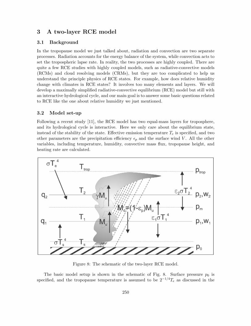
Following a recent study [11], the RCE model has two equal-mass layers for troposphere,and its hydrological cycle is interactive. Here we only care about the equilibrium state,instead of the stability of the state. Effective emission temperature Te is specified, and twoother parameters are the precipitation efficiency εp and the surface wind V . All the othervariables, including temperature, humidity, convective mass flux, tropopause height, andheating rate are calculated.

Figure 8: The schematic of the two-layer RCE model.

The basic model setup is shown in the schematic of Fig. 8. Surface pressure p0 isspecified, and the tropopause temperature is assumed to be 2−1/4Te as discussed in the

250

previous section. In the following discussions, the subscripts ‘1’, ‘2’, ‘s’, ‘b’, ‘m’, and ‘trop’stand for the lower layer, upper layer, surface, boundary layer, middle of troposphere, andtropopause, respectively. Note that ‘middle’ indicates the mid-level in terms of mass – inother words, in the pressure coordinate.

Let’s start with the energy balance in the two layers. In the lower layer,

Fs −Mu(hb − hm) +Q1 = 0, (3.1)

where Fs is the surface turbulent enthalpy flux, Mu is the convective mass flux, hb and hmis the moist static energy (MSE) in the middle of troposphere and in the subcloud layer,and Q1 is the radiative cooling. Surface turbulent enthalpy flux is essentially determinedby surface wind speed, surface saturation specific humidity, and surface relative humidity,

Fs = V (hs − hb) ≈ V Lvq∗s(1−Hs), (3.2)

where V is defined asV = ρbCkV. (3.3)

Similarly, in the upper layer,Mu(hb − hm) +Q2 = 0, (3.4)

where we assume the MSE at the tropopause is the same as that in the subcloud layer, sothere is no MSE exchange at the tropopause.

Energy balance should also hold in the clear air between clouds. In the lower layer,assuming convective downdraft as (1− εp)Mu, we can have that the large-scale subsidencein the clear air is εpMu. So the energy balance can be written as

εpMu∆S1 +Q1 = 0, (3.5)

where we are assuming convection only occupies a very small portion of the domain area,and ∆S1 is the contrast in dry static energy between the mid-troposphere and the surface,

∆S1 = cp(Tm − Ts) + gzm. (3.6)

Similarly, we can write the energy balance in the clear air of upper layer as,

γMu∆S2 +Q2 = 0, (3.7)

where ∆S2 is the contrast in dry static energy between the tropopause and the mid-troposphere,

∆S2 = cp(Ttrop − Tm) + g(ztrop − zm). (3.8)

Note that here γ, not like εp, is calculated instead of specified, so it is not a parameter.Finally let’s consider the energy balance in the subcloud layer and at the surface. In

the subcloud layer, surface turbulent enthalpy flux is balanced by the convective flux outof the layer and the flux due to shallow convection; that is,

Mu(hb − hm) + Fshallow = Fs. (3.9)

251

If we parameterize Fshallow as (1− α)Fs, we can then get

Mu(hb − hm) = αFs. (3.10)

Note that here α is calculated, not a parameter. The surface energy balance requires that

Fs −Qs = 0. (3.11)

The radiative heating rates in the lower layer, the upper layer, and at the surface canbe defined as,

Q1 = σε1(T4s − 2T 4

1 + ε2T42 ), (3.12)

Q2 = σε2[(1− ε1)T 4s − 2T 4

2 + ε1T41 ], (3.13)

Qs = σ[T 4e + ε1T

41 + ε2(1− ε1)T 4

2 − T 4s ]. (3.14)

In addition to those three sets of energy balance equations, we also need to make as-sumptions of conserved saturation MSE and saturation entropy in the whole column, whichare controlled by subcloud properties. Mathematically, it can be expressed as,

hb = h∗1 = h∗m = h∗2 = h∗trop (3.15)

andsb = s∗1 = s∗m = s∗2 = s∗trop. (3.16)

Since this is a highly coupled and nonlinear system, we need to solve it numerically.Numerical solutions will be discussed in the following subsections.

3.3 State-dependent emissivity

Before we talk about the solutions, one thing we want to emphasize is the state-dependenceof layer emissivities. Intuitively, we can imagine that when water vapor increases in a certainlayer, more longwave radiation can be absorbed or emitted given a certain temperature; inother words, layer emissivity will increase. But, quantitively determining the relationshipbetween emissivity and water vapor (or temperature) is not a trivial problem. As a first step,we can try to use an artificial exponential function to mimic the Clausius-Clapeyron relation,but the parameters we will choose are quite empirical. We notice that this relation is a keyelement coupling radiation and convection, so it will largely affect the model behavior.Thus, we decide to use more realistic formulation to get a more reasonable model behavior.

Following a very early study [12], we seek to find a relation between layer emissivity andwater vapor path (WVP, sometimes also called total precipitable water, defined as the heightof water if all water vapor in a certain layer condenses to liquid water). Carbon dioxidehas been taken into account, but its concentration is held as constant around 400ppmv.The overlap of absorption spectrum between water vapor and carbon dioxide has also beencorrected. Results are shown in Fig. 9. The WVP of current earth is about 27mm, rangingfrom 1mm in the polar regions to 42mm in the tropics, so the layer emissivity is roughly inthe range of 0.6 to 0.8.

252

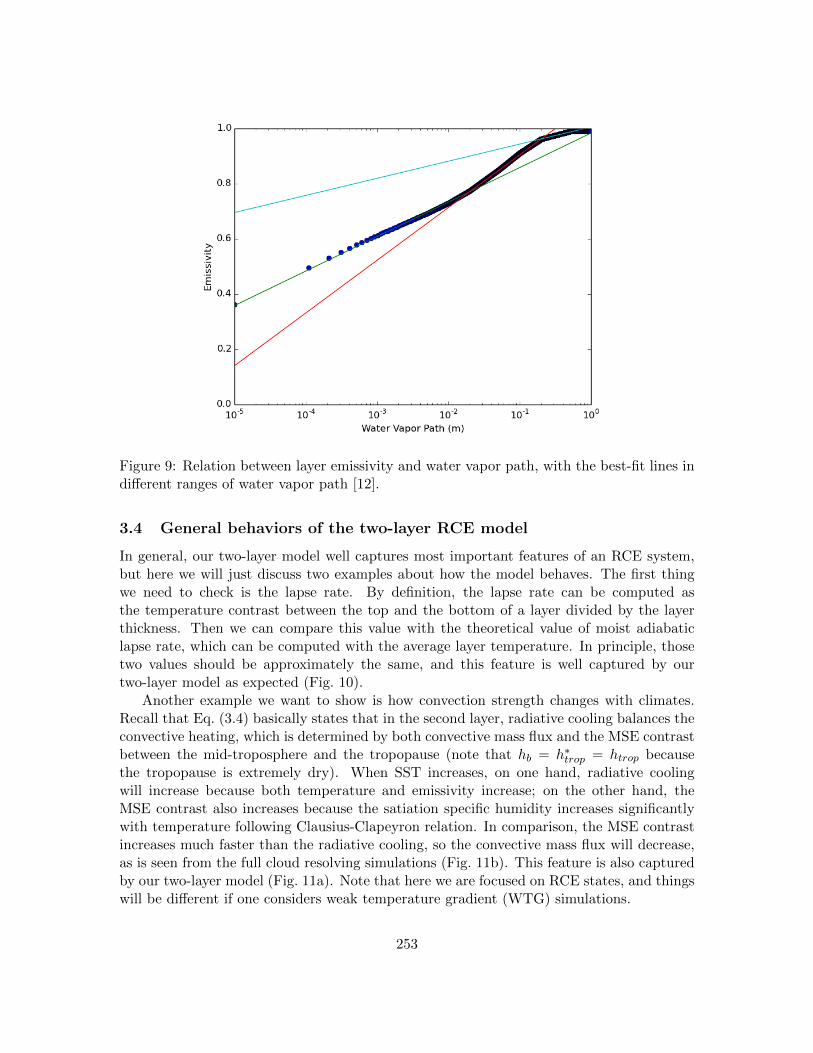
Figure 9: Relation between layer emissivity and water vapor path, with the best-fit lines indifferent ranges of water vapor path [12].

3.4 General behaviors of the two-layer RCE model

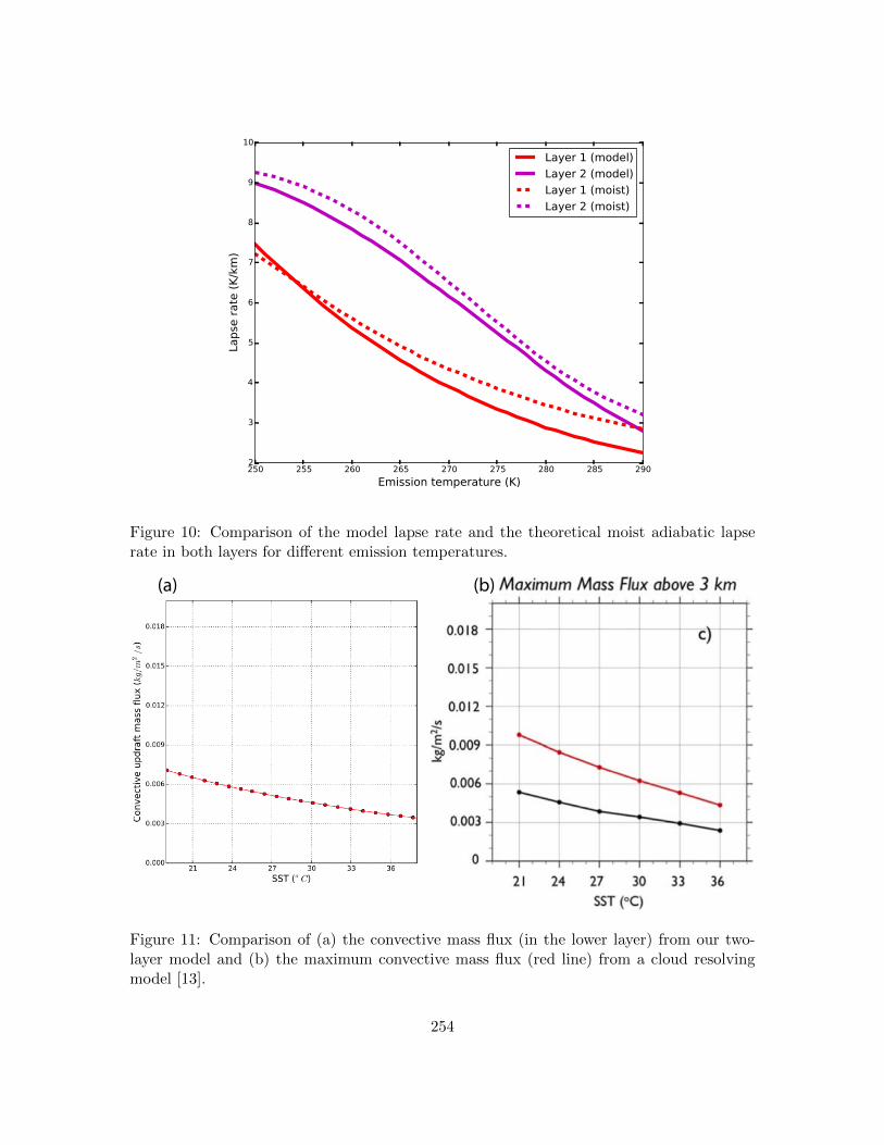
In general, our two-layer model well captures most important features of an RCE system,but here we will just discuss two examples about how the model behaves. The first thingwe need to check is the lapse rate. By definition, the lapse rate can be computed asthe temperature contrast between the top and the bottom of a layer divided by the layerthickness. Then we can compare this value with the theoretical value of moist adiabaticlapse rate, which can be computed with the average layer temperature. In principle, thosetwo values should be approximately the same, and this feature is well captured by ourtwo-layer model as expected (Fig. 10).

Another example we want to show is how convection strength changes with climates.Recall that Eq. (3.4) basically states that in the second layer, radiative cooling balances theconvective heating, which is determined by both convective mass flux and the MSE contrastbetween the mid-troposphere and the tropopause (note that hb = h∗trop = htrop becausethe tropopause is extremely dry). When SST increases, on one hand, radiative coolingwill increase because both temperature and emissivity increase; on the other hand, theMSE contrast also increases because the satiation specific humidity increases significantlywith temperature following Clausius-Clapeyron relation. In comparison, the MSE contrastincreases much faster than the radiative cooling, so the convective mass flux will decrease,as is seen from the full cloud resolving simulations (Fig. 11b). This feature is also capturedby our two-layer model (Fig. 11a). Note that here we are focused on RCE states, and thingswill be different if one considers weak temperature gradient (WTG) simulations.

253

250 255 260 265 270 275 280 285 290

Emission temperature (K)

2

3

4

5

6

7

8

9

10

Lapse

rate

(K

/km

)

Layer 1 (model)

Layer 2 (model)

Layer 1 (moist)

Layer 2 (moist)

Figure 10: Comparison of the model lapse rate and the theoretical moist adiabatic lapserate in both layers for different emission temperatures.

(a) (b)

Figure 11: Comparison of (a) the convective mass flux (in the lower layer) from our two-layer model and (b) the maximum convective mass flux (red line) from a cloud resolvingmodel [13].

254

3.5 How does relative humidity change with climates from an RCE per-spective?

How relative humidity changes with climates is a fundamental and important question,but we still lack a complete answer to that. Some studies regard it as a constant variablein climate models, but this assumption still needs to be justified. Among all argumentsrelated to this question, large-scale circulation argument might be known and accepted bymost people in the community. It basically states that large-scale circulation transports asaturated air parcel to a warmer place, which makes it under-saturated, and the relativehumidity is simply determined by the temperature difference between two places; thereforeas long as the large-scale circulation does’t change too much, global (or tropical) averagerelative humidity in the troposphere might not be able to change too much. Here we willfocus on RCE states without any large-scale circulation, and our results suggest that evenin RCE states, tropospheric relative humidity can not change much and a key element isthe radiation-convection coupling.

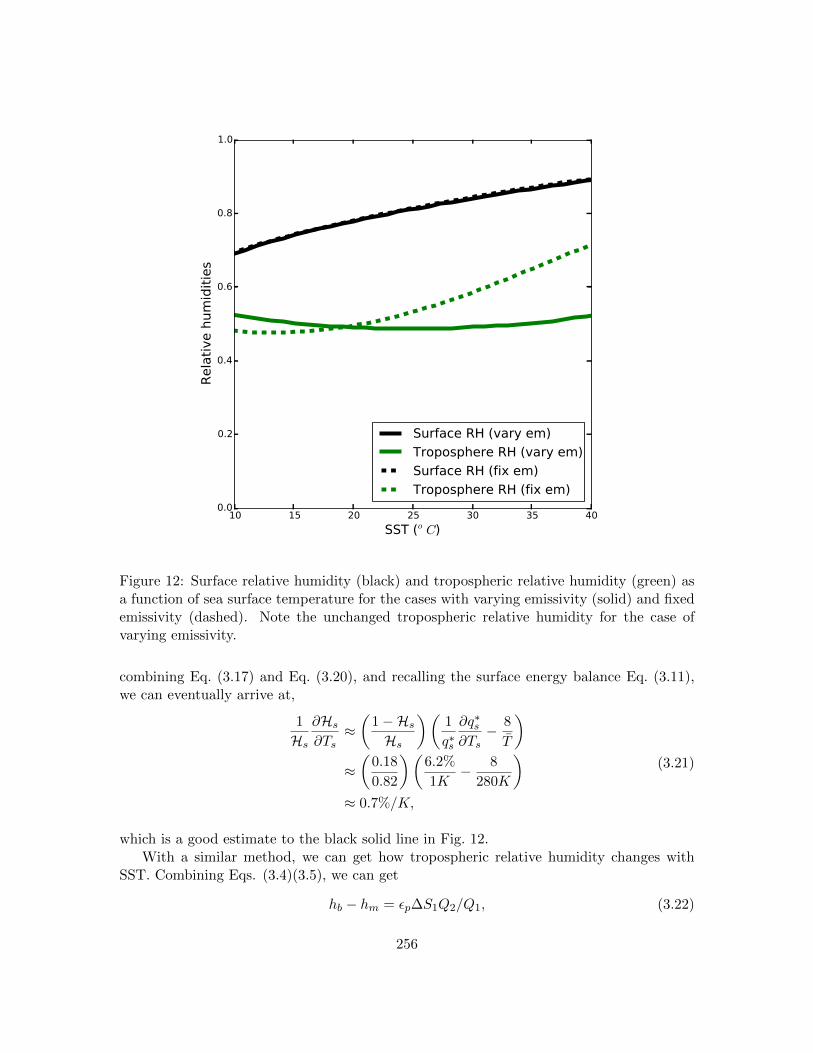
Seen from our two-layer model results, tropospheric relative humidity hardly changeswithin a broad range of SST. When SST increases from 10oC to 40oC, surface relativehumidity slowly increases from 0.7 to 0.9; however, the relative humidity in the free tropo-sphere changes little and sits at a value of 0.5. To better understand this behavior, we willmake use of the energy balance equations mentioned above and conduct energetics analysis.

Let’s start with the surface relative humidity. From Eq. (3.2), we can easily get

1

Fs

∂Fs

∂Ts=

1

q∗s

∂q∗s∂Ts−( Hs

1−Hs

)1

Hs

∂Hs

∂Ts, (3.17)

Similarly, from Eq. (3.14), we can get

1

Qs

∂Qs

∂Ts=A+B

C, (3.18)

where

A = 4[T 3e

∂Te∂Ts

+ ε1T31

∂T1∂Ts

+ ε2(1− ε1)T 32

∂T2∂Ts− T 3

s ],

B =∂ε1∂Ts

T 41 + [(1−ε1)

∂ε2∂Ts− ε2

∂ε1∂Ts

]T 42 ,

C = T 4e + ε1T

41 +ε2(1− ε1)T 4

2 − T 4s .

(3.19)

Since layer emissivity is close to 1, the second term B/C is relatively small compared withA/C and can be neglected. Then we can simplify Eq. (3.18) as

1

Qs

∂Qs

∂Ts≈ 4

T

∂T

∂Ts≈ 8

T(3.20)

where T is the average tropospheric temperature, and it is roughly 280K when surfacetemperature is 300K. The second approximation is because the value of ∂T /∂Ts can beassumed to be 2, which indicates that, given a certain increase in surface temperature,tropospheric temperature is amplified by a factor of 2 due to the lapse rate feedback. Then

255

10 15 20 25 30 35 40

SST (o C)

0.0

0.2

0.4

0.6

0.8

1.0

Rela

tive h

um

idit

ies

Surface RH (vary em)

Troposphere RH (vary em)

Surface RH (fix em)

Troposphere RH (fix em)

Figure 12: Surface relative humidity (black) and tropospheric relative humidity (green) asa function of sea surface temperature for the cases with varying emissivity (solid) and fixedemissivity (dashed). Note the unchanged tropospheric relative humidity for the case ofvarying emissivity.

combining Eq. (3.17) and Eq. (3.20), and recalling the surface energy balance Eq. (3.11),we can eventually arrive at,

1

Hs

∂Hs

∂Ts≈(

1−Hs

Hs

)(1

q∗s

∂q∗s∂Ts− 8

T

)

≈(

0.18

0.82

)(6.2%

1K− 8

280K

)

≈ 0.7%/K,

(3.21)

which is a good estimate to the black solid line in Fig. 12.With a similar method, we can get how tropospheric relative humidity changes with

SST. Combining Eqs. (3.4)(3.5), we can get

hb − hm = εp∆S1Q2/Q1, (3.22)

256

and thus1

hb − hm∂(hb − hm)

∂Ts=

1

Q2

∂Q2

∂Ts− 1

Q1

∂Q1

∂Ts+

1

∆S1

∂∆S1∂Ts

. (3.23)

Then we rewrite (hb − hm) as

hb − hm = h∗m − hm = Lvq∗m(1−Hm). (3.24)

Also, we rewrite ∆S1 as

∆S1 = (h∗m − Lvq∗m)− (hb − Lvqs) = Lv(q∗sHs − q∗m). (3.25)

Substituting Eqs.(3.24)(3.25) into Eq.(3.23), we get

1

Hm

∂Hm

∂Ts=

(1−Hm

Hm

)[1

q∗m

∂q∗m∂Ts

− 1

q∗sHs − q∗m∂(q∗sHs − q∗m)

∂Ts+

1

Q1

∂Q1

∂Ts− 1

Q2

∂Q2

∂Ts

]

(3.26)

When layer emissivity varies with SST (or WVP), the three terms in Eq. (3.26) are

1

q∗m

∂q∗m∂Ts

≈ 9.4%/K, (3.27)

− 1

q∗sHs − q∗m∂(q∗sHs − q∗m)

∂Ts≈ −4.4%/K, (3.28)

1

Q1

∂Q1

∂Ts− 1

Q2

∂Q2

∂Ts≈ −5.0%/K, (3.29)

which are the values when SST is 300K. Substituting Eqs.(3.27)(3.28)(3.29) into Eq.(3.26),we get

1

Hm

∂Hm

∂Ts≈ 0.0%/K. (3.30)

That is why tropospheric relative humidity changes little with a broad range of climate withSST varying from 10oC to 40oC.

Since this RCE system is highly coupled, it is hard to say which single element inthis coupled system causes the almost constant tropospheric relative humidity. Actually,it is due to the radiation-convection coupling itself, in other words, the feedback betweenradiation and convection. To test this hypothesis, we can fix the layer emissivity to aconstant value, which kills the coupling between convection and radiation, and see how therelative humidity changes with SST.

Interestingly, we find that the case with fixed emissivity experiences a significant increasein the tropospheric relative humidity with SST. This can be partly explained by the sameenergetics analysis we conducted above, and the new values of the three terms in Eq. (3.26)are

1

q∗m

∂q∗m∂Ts

≈ 9.4%/K, (3.31)

257

(a) (b)

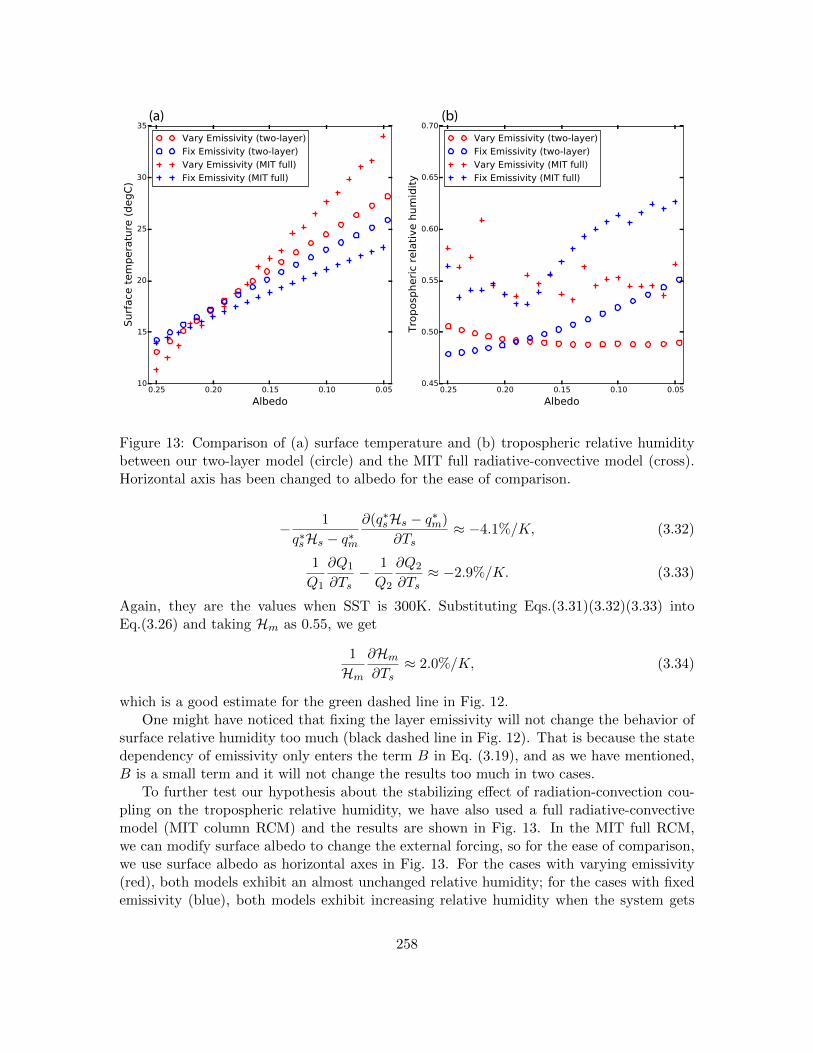
Figure 13: Comparison of (a) surface temperature and (b) tropospheric relative humiditybetween our two-layer model (circle) and the MIT full radiative-convective model (cross).Horizontal axis has been changed to albedo for the ease of comparison.

− 1

q∗sHs − q∗m∂(q∗sHs − q∗m)

∂Ts≈ −4.1%/K, (3.32)

1

Q1

∂Q1

∂Ts− 1

Q2

∂Q2

∂Ts≈ −2.9%/K. (3.33)

Again, they are the values when SST is 300K. Substituting Eqs.(3.31)(3.32)(3.33) intoEq.(3.26) and taking Hm as 0.55, we get

1

Hm

∂Hm

∂Ts≈ 2.0%/K, (3.34)

which is a good estimate for the green dashed line in Fig. 12.One might have noticed that fixing the layer emissivity will not change the behavior of

surface relative humidity too much (black dashed line in Fig. 12). That is because the statedependency of emissivity only enters the term B in Eq. (3.19), and as we have mentioned,B is a small term and it will not change the results too much in two cases.

To further test our hypothesis about the stabilizing effect of radiation-convection cou-pling on the tropospheric relative humidity, we have also used a full radiative-convectivemodel (MIT column RCM) and the results are shown in Fig. 13. In the MIT full RCM,we can modify surface albedo to change the external forcing, so for the ease of comparison,we use surface albedo as horizontal axes in Fig. 13. For the cases with varying emissivity(red), both models exhibit an almost unchanged relative humidity; for the cases with fixedemissivity (blue), both models exhibit increasing relative humidity when the system gets

258

warmer. Those trends agree especially well when albedo is in the range of 0.05 to 0.20,and surface temperature is in the range of 15oC to 30oC, which is exactly the temperaturerange of current tropics.

4 Conclusions and discussions

This study develops two idealized models with different simplifications from the full radiative-convective equilibrium system. The first model is a one-dimensional tropopause model withmultiple layers but less coupling. We find that this 1-D model, even without any explicitdynamics, can well reproduce the observed meridional structure of tropopause height, andcan also explain why the tropical tropopause is higher, colder, and sharper than the extrat-ropical tropopause. Brewer-Dobson circulation is a key element in explaining the observedfeatures of the tropopause. We will use an idealized GCM to further test this hypothesis.

The second model is a two-layer RCE model with interactive hydrological cycle. Thisextremely simplified model captures the main features of RCE states very well, and itssimplicity helps us better understand the basic physics of RCE. With this model, we findthat tropospheric relative humidity hardly changes climate in a broad range of SST from15oC to 30oC, which is exactly the temperature range of current tropics. We want toemphasize that it is an alternative argument, aside from the conventional argument withlarge-scale circulation, on explaining the unchanged relative humidity with climates peopleusually assume. The key element of this argument is the coupling between radiation andconvection. Once we kill this coupling or use an unrealistic relation between emissivity andwater vapor path, we might fail to observe this phenomenon.

For future investigation, we are hoping to combine the two simplified models to betterunderstand how the height of tropopause changes with climate (temperature, humidity,etc.), and going further, large-scale circulation such as lateral transport and mid-latitudeeddies will be incorporated in the model as well to form a full picture.

Acknowledgements

I would like to thank Geoff Vallis and Kerry Emanuel for suggesting this wonderful project,for their invaluable guidance, and continuous supervision throughout the summer. I alsowould like to thank Andy Ingersoll for a lot of insightful discussions. Thanks also to thedirectors for organizing a smooth program. Last, but certainly not least, I would like tothank all Fellows for a memorable summer.

References

[1] G Vaughan and JD Price. On the relation between total ozone and meteorology.Quarterly Journal of the Royal Meteorological Society, 117(502):1281–1298, 1991.

[2] James R Holton, Peter H Haynes, Michael E McIntyre, Anne R Douglass, Richard BRood, and Leonhard Pfister. Stratosphere-troposphere exchange. Reviews of Geo-physics, 33(4):403–439, 1995.

259

[3] LJ Wilcox, BJ Hoskins, and KP Shine. A global blended tropopause based on eradata. part i: Climatology. Quarterly Journal of the Royal Meteorological Society,138(664):561–575, 2012.

[4] Geoffrey K Vallis. Atmospheric and oceanic fluid dynamics: fundamentals and large-scale circulation. Cambridge University Press, 2006.

[5] Issac M Held. On the height of the tropopause and the static stability of the tropo-sphere. Journal of the Atmospheric Sciences, 39(2):412–417, 1982.

[6] Pablo Zurita-Gotor and Geoffrey K Vallis. Determination of extratropical tropopauseheight in an idealized gray radiation model. Journal of the Atmospheric Sciences,70(7):2272–2292, 2013.

[7] Peter H Stone and John H Carlson. Atmospheric lapse rate regimes and their param-eterization. Journal of the Atmospheric Sciences, 36(3):415–423, 1979.

[8] II Mokhov and MG Akperov. Tropospheric lapse rate and its relation to surface temper-ature from reanalysis data. Izvestiya, Atmospheric and Oceanic Physics, 42(4):430–438,2006.

[9] Dargan MW Frierson, Isaac M Held, and Pablo Zurita-Gotor. A gray-radiation aqua-planet moist gcm. part i: Static stability and eddy scale. Journal of the atmosphericsciences, 63(10):2548–2566, 2006.

[10] Paul A O’Gorman and Tapio Schneider. The hydrological cycle over a wide range ofclimates simulated with an idealized gcm. Journal of Climate, 21(15):3815–3832, 2008.

[11] Kerry Emanuel, Allison A Wing, and Emmanuel M Vincent. Radiative-convectiveinstability. Journal of Advances in Modeling Earth Systems, 6(1):75–90, 2014.

[12] DO Staley and GM Jurica. Flux emissivity tables for water vapor, carbon dioxide andozone. Journal of Applied Meteorology, 9(3):365–372, 1970.

[13] Marat Khairoutdinov and Kerry Emanuel. Rotating radiative-convective equilibriumsimulated by a cloud-resolving model. Journal of Advances in Modeling Earth Systems,5(4):816–825, 2013.

260