Embed Size (px)
Citation preview

Models for managing surge capacity in the face of an influenzaepidemic
Ana Cecilia Zenteno Langle
Submitted in partial fulfillment of the
Requirements for the degree
of Doctor of Philosophy
in the Graduate School of Arts and Sciences
COLUMBIA UNIVERSITY
2013

c©2013
Ana Cecilia Zenteno Langle
All Rights Reserved

ABSTRACT
Models for managing surge capacity in the face of an influenzaepidemic
Ana Cecilia Zenteno Langle
Influenza pandemics pose an imminent risk to society. Yearlyoutbreaks already represent heavy social
and economic burdens to society. A pandemic could severely affect infrastructure and commerce through
high absenteeism, supply chain disruptions, and other effects over an extended and uncertain period of
time. Governmental institutions such as the Center for Disease Prevention and Control (CDC) and the U.S.
Department of Health and Human Services (HHS) have issued guidelines on how to prepare for a potential
pandemic, however much work still needs to be done in order tomeet them. from a planner’s perspective, the
complexity of outlining plans to manage future resources during an epidemic stems from the uncertainty of
how severe the epidemic will be. Uncertainty in parameters such as the contagion rate (how fast the disease
spreads) makes the course and severity of the epidemic unforeseeable, exposing any planning strategy to a
potentially wasteful allocation of resources.
In this thesis we consider robust models of surge capacity planning. We focus on surge staff deployment
strategies that aim to mitigate the impact of an influenza epidemic on an organization’s operations. Our
approach involves the use of additional resources in response to a robust model of the evolution of the
epidemic as to hedge against the uncertainty in its evolution and intensity. Under existing plans, large cities

would make use of networks of volunteers, students, and recent retirees, or “borrow” staff from neighboring
communities. Taking into account that such additional resources are likely to be significantly constrained
(e.g. in quantity and duration), we seek to produce robust emergency staff commitment levels that workwell
under different trajectories and degrees of severity of thepandemic.
Our methodology combines Robust Optimization techniques with Epidemiology (SEIR models) and system
performance modeling. We describe cutting-plane algorithms analogous to generalized Benders’ decom-
position that prove fast and numerically accurate. Our results yield insights on the structure of optimal
robust strategies and on practical rules-of-thumb that canbe deployed during the epidemic. To assess the
efficacy of our solutions, we study their performance under different scenarios and compare them against
other seemingly good strategies through numerical experiments.
This work would be particularly valuable for institutions that provide public services, whose operations
continuity is critical for a community, especially in view of an event of this caliber. As far as we know, this
is the first time this problem is addressed in a rigorous way; particularly we are not aware of any other robust
optimization applications in epidemiology.

Table of Contents
Table of Contents
List of Figures iv
Acknowledgments v
Chapter 1: Introduction 1
Chapter 2: Preliminaries 5
2.1 Operations Research and Public Health. . . . . . . . . . . . . . . . . . . . . . . . . . . . . 5
2.2 Influenza virus and pandemics. . . . . . . . . . . . . . . . . . . . . . . . . . . . . . . . . 6
2.2.1 Pandemic Preparedness. . . . . . . . . . . . . . . . . . . . . . . . . . . . . . . . . 9
2.3 Robust Optimization and Benders’ Decomposition. . . . . . . . . . . . . . . . . . . . . . 11
Chapter 3: Contingency Planning 14
3.1 Planning for workforce shortfall. . . . . . . . . . . . . . . . . . . . . . . . . . . . . . . . 14
3.2 Declaring an epidemic. . . . . . . . . . . . . . . . . . . . . . . . . . . . . . . . . . . . . 18
i

Table of Contents
Chapter 4: Modeling Influenza 20
4.1 Modeling literature . . . . . . . . . . . . . . . . . . . . . . . . . . . . . . . . . . . . . . . 20
4.2 SEIR model. . . . . . . . . . . . . . . . . . . . . . . . . . . . . . . . . . . . . . . . . . . 22
4.3 Robustness in planning. . . . . . . . . . . . . . . . . . . . . . . . . . . . . . . . . . . . . 29
Chapter 5: Robust Models 35
5.1 Performance Measures. . . . . . . . . . . . . . . . . . . . . . . . . . . . . . . . . . . . . 35
5.1.1 Threshold functions. . . . . . . . . . . . . . . . . . . . . . . . . . . . . . . . . . . 36
5.1.2 Queueing models. . . . . . . . . . . . . . . . . . . . . . . . . . . . . . . . . . . . 36
5.1.3 Other cost functions. . . . . . . . . . . . . . . . . . . . . . . . . . . . . . . . . . 37
5.2 Robust Models . . . . . . . . . . . . . . . . . . . . . . . . . . . . . . . . . . . . . . . . . 38
5.2.1 Uncertainty models. . . . . . . . . . . . . . . . . . . . . . . . . . . . . . . . . . . 38
5.2.2 Deployment strategies. . . . . . . . . . . . . . . . . . . . . . . . . . . . . . . . . 40
5.2.3 Robust problem. . . . . . . . . . . . . . . . . . . . . . . . . . . . . . . . . . . . . 44
Chapter 6: Numerical Experiments 46
6.1 Examples in a health care setting. . . . . . . . . . . . . . . . . . . . . . . . . . . . . . . . 47
6.1.1 Example 1 . . . . . . . . . . . . . . . . . . . . . . . . . . . . . . . . . . . . . . . 47
6.1.2 Example 2 . . . . . . . . . . . . . . . . . . . . . . . . . . . . . . . . . . . . . . . 57
6.1.3 Out-of-sample tests. . . . . . . . . . . . . . . . . . . . . . . . . . . . . . . . . . . 61
ii

Table of Contents
Chapter 7: Solving the Robust Problem 72
7.1 The robust problem as an infinite linear program. . . . . . . . . . . . . . . . . . . . . . . . 73
7.2 Algorithm . . . . . . . . . . . . . . . . . . . . . . . . . . . . . . . . . . . . . . . . . . . . 77
7.2.1 Implementation. . . . . . . . . . . . . . . . . . . . . . . . . . . . . . . . . . . . . 79
7.3 Improved algorithm. . . . . . . . . . . . . . . . . . . . . . . . . . . . . . . . . . . . . . . 84
7.3.1 Example 1 Revisited. . . . . . . . . . . . . . . . . . . . . . . . . . . . . . . . . . 87
Chapter 8: Extensions 91
8.1 Robust optimization with recourse. . . . . . . . . . . . . . . . . . . . . . . . . . . . . . . 92
8.2 Stochastic optimization. . . . . . . . . . . . . . . . . . . . . . . . . . . . . . . . . . . . . 93
Chapter 9: Discussion 97
iii

List of Figures
List of Figures
4.1 BasicSEIR model. . . . . . . . . . . . . . . . . . . . . . . . . . . . . . . . . . . . . . . 24
4.2 Two parallelSEIR models. . . . . . . . . . . . . . . . . . . . . . . . . . . . . . . . . . . 26
4.3 Availability of workforce as epidemic progresses for different values ofp. . . . . . . . . . . 31
4.4 Availability of workforce whenp is allowed to changeduring the epidemic. . . . . . . . . . 33
6.1 Ex 1. Reduction inρ obtained by Robust and Naïve-worst-case strategies.. . . . . . . . . . 66
6.2 Ex 1. Deployment strategies for different smoothing tolerances. . . . . . . . . . . . . . . . 67
6.3 Ex 1. Deployment strategies for different discretizations of the uncertainty set.. . . . . . . . 67
6.4 Ex 1. Changes in workforce availability after deployment of strategies.. . . . . . . . . . . . 68
6.5 Ex 2. Structure of the Robust and Naïve-worst-case deployment strategies.. . . . . . . . . . 68
6.6 Ex 2. Change in strategies’ structure for different amounts of available surge staff.. . . . . . 69
6.7 Ex 2. Cost of an epidemic as a function ofp. . . . . . . . . . . . . . . . . . . . . . . . . . . 69
6.8 Ex 1. Out-of-sample testing.. . . . . . . . . . . . . . . . . . . . . . . . . . . . . . . . . . 70
6.9 Ex 2. Out-of-sample testing: Implementing the strategyn days late. . . . . . . . . . . . . . 71
7.1 Ex 1 - Cont’d. Deployment strategy for improved algorithm with queueing objective.. . . . 89
7.2 Ex 1 - Cont’d. Deployment strategy for improved algorithm with threshold objective.. . . . 90
iv

Acknowledgments
Acknowledgments
I would like to start by thanking my advisor, Prof. Daniel Bienstock, whose support was a key element to
the advancement of this thesis and my doctorate. Not only is he smart, he is encouraging, funny, extremely
patient, and deeply concerned about his students’ wellbeing.
Other professors to whom I am indebted for their contribution to my personal and professional development
are Professors Garud Iyengar, Ward Whitt, and Don Goldfarb.They all lead by example. I would also
like to thank Professor Maria Chudnovsky; working as her Teaching Assistant was very enjoyable and very
nurturing.
I am also grateful to the department staff, who was always happy to attend my numerous requests. Donella,
Maria, Jaya, Jenny, Risa, Darbi, Aysha, Shi Yee, Adina, Michael; they were always helpful and responsive.
My most sincere appreciation goes for all the good friends I met these past five years. They made the
good times merrier and the hard times bearable, becoming an essential part of my life in New York. It is
impossible to quantify how much I have learned from them. Special thanks go to my officemates at Mudd
313A and at Schapiro 821, with whom I shared so many hours of myPh.D. Running the terrible risk of
forgetting someone, I want to mention Yori, Romain, Rodrigo, Dani, Silvi, Vero, Majo, Jing, Song-hee,
Tulia, Matthieu, María de la Garza, Elia, Colin; I will always cherish all the laughs we shared. Very special
v

Acknowledgments
thanks go to Angel Almada and Raúl González, for being alwayswith me, no matter the distance. I am
thankful to Angel for his constant push to go beyond what I think is possible and for having patiently listened
to my endless whining. I thank Yixitín for watching my back (literally and figuratively) for four precious
years. I am ever grateful to Bar Ifrach, for the long-lastingfriendship we built from the first recitation we
attended; I am particularly fond of his caring and honest advice. I am especially beholden to Rouba Ibrahim
for her constant kindness and most encouraging support; shemust be the most warm hearted person I know.
I owe my deepest gratitude to my family in Mexico, particularly my mom, my dad, Dany, and Raúl. Being
far away from them continues to be one of the most difficult challenges I have faced. Their love and support
were pivotal during the whole of my graduate studies. Their hard work and generosity will forever be a
source of inspiration.
This thesis and my doctorate studies in general would have never been possible without Filippo Balestrieri.
His unbreakable faith in me carried me through the toughest times; his seemingly infinite wittinessalways
finds a way to make me smile. I love him with all my being. This thesis is dedicated to him.
vi

Chapter 1. Introduction 1
11Introduction
In this paper we consider robust models for emergency staff deployment in the event of a flu pandemic. We
focus on managing critical staff levels at organizations that must remain operational during such an event,
and develop methodologies for managing emergency resources with the goal of minimizing the impact of the
pandemic. We present numerical experiments using realistic data to study the effectiveness of our approach.
A serious flu epidemic or pandemic, particularly one characterized by high contagion rate, would have
extremely damaging impact on a large, dense population center. The 1918 influenza pandemic is often seen
as a worst-case scenario as it arguably represents the most devastating pandemic in recent history, having
killed more than 20 million people worldwide[20, 53, 71]. However, even a much milder epidemic would
have vast social impact as services such as health care, police and utilities became severely hampered by
staff shortages. Workplace absenteeism might also become aserious concern[72]. In the United States, the
Implementation Plan for the National Strategy for PandemicInfluenza foresee absenteeism levels as high as

Chapter 1. Introduction 2
40% at the height of the pandemic wave ([40]). In the health care setting, there are mixed views: While some
preparedness plans project high absenteeism due to illnessor need to care for family members ([57]), the
opposite may also take place: health care workers may reportedly avoid calling in sick during an emergency
as observed during the last H1N1 outbreak[27, 16].
In this study we focus on managing the inevitable staff shortfall that will take place in the case of a severe
epidemic. We take the viewpoint of an organization that seeks to diminish decreased performance in its
operations as the epidemic unfolds, by appropriately deploying available resources, but which is not directly
attempting to control the number of people that become infected. Some examples of infrastructure of critical
social value we are interested in are hospitals, police departments, power plants and supply chains; these
are entities that must remain operative even as staff levelsbecome low. In cases such as police departments,
staff would likely be more exposed to the epidemic than the general public and (particularly if vaccines
are in short supply, or apply to the wrong virus mutation) shortfalls may take place just when there is
greatest demand for services. Power plants and waste water treatment plants are examples of facilities
whose operation will be degraded as staff falls short and which probably require minimum staff levels to
operate at all[39]. Supply chains would very likely be significantly slowed down as their staff is depleted,
resulting, for example, in food shortages[66]. In all these cases, organizations cannot implement “work
from home” strategies as urged for private businesses by theCenters of Disease Control and Prevention
(CDC) and the United States Department of Labor[63].
In contrast to our focus, much valuable research has been directed at addressing the epidemic itself. Such
work studies public health measures that would reduce the epidemic’s severity and its direct impact, for
example by managing the supply of vaccines and antivirals (see[50, 38, 51]). While we do not address this
topic, it seems plausible that robust optimization techniques could be applied in these settings, as well. To

Chapter 1. Introduction 3
the best of our knowledge this is the first time that these methodologies are introduced into this research
area.
A pandemic contingency plan for a large organization (such as a city government) would include resorting
to emergency (or “surge”) sources for additional staff: forexample by temporarily relying on personnel
from outlying, less dense, communities. Such additional resources are likely to be significantly constrained
in quantity, duration and rate, among other factors. Such emergency staff deployment plans would entail
some complexity in design, calibration and implementation, but as a result of other disasters such, as Hur-
ricane Katrina in 2005 and the anthrax attacks in 2001, it is now agreed that there is a compelling need for
emergency planning[30].
From a planner’s perspective, the task of managing future resource levels during an epidemic is complex,
partly because of uncertainties regarding the behavior of the epidemic, in particular, uncertainty in the con-
tagion rate. The evolution of the contagion rate is a function of poorly understood dynamics in the mutations
of the different strains of the flu virus and environmental agents such as weather[20, 52]. Additionally, non-
pharmaceutical public health interventions such as quarantine and social distancing could impose significant
changes in social contact patterns that would in turn affectthe contagion rate. In addition to uncertainty, a
decision-maker will also likely be constrained by logistics. In particular, it may prove impossible to carry out
large changes to staff deployment plans on short notice, particularly if such staff is also in demand by other
organizations (as might be the case during a severe epidemic). We will return to these issues in Sections
5.2.2and8. As a consequence of the two factors (uncertainty, and logistical constraints) a decision-maker
may commit too few or too many resources - in this case emergency staff- or perhaps at the wrong time, if
there turns out to be a mismatch between the anticipated level of staff shortage and what actually transpires
(after the resources have been committed).
Chapter 1. Introduction 4
We present models and methodology for developing emergencystaff deployment levels which optimally
hedge against the uncertainty in the evolution an the epidemic while accounting for operational constraints.
Our approach overlays adversarial models on the classical SEIR model for describing epidemics to charac-
terize the potentially wide variability of the contagion rate. The resulting robust optimization models are
non-convex and large-scale; we present convex approximations and algorithms that empirically prove nu-
merically accurate and efficient, and we study their behavior and the policies they produce under a range of
scenarios.
This thesis is organized as follows. Chapter2 contains preliminaries to the main topics addressed in this
work. Issues related to surge capacity planning are described in Chapter3; Chapter4 describes the classical
SEIR model and makes the case for robustness. Chapter5 contains the description of our robust model and
Chapter6 presents the results of our numerical experiments; detailsof the robust algorithm are presented in
Chapter7. We discuss extensions and give final remarks in Chapters8 and9, respectively.

Chapter 2. Preliminaries 5
22Preliminaries
2.1 Operations Research and Public Health
Operations Research is the science of better decision making. It provides a structured framework to analyze
complex systems by capturing their main uncertainties and interactions. While the field originally had
military applications, it is now prevalent in supply chain management, transportation, services and, more
recently, homeland security and health care management.
Public Health studies how to protect and improve the health of communities through education, promotion
of healthy lifestyles, and research for disease and injury prevention[81]. Typical Public Health programs
include disease screening and surveillance (such as HIV andinfluenza), vaccination, outbreak investiga-
tion (SARS), inspection and standard enforcement at publicestablishments, environmental monitoring, and
vector control (mosquitoes, ticks that transmit diseases)[41].

Chapter 2. Preliminaries 6
Like any other services, Public Health programs require adequate design and effective implementation to
have the desired impact. Herein lie many opportunities to apply Operations Research principles and tech-
niques: the delineation, evaluation and operation of theseservices may benefit significantly from inter-
weaving theoretical insight with practical experience which no health worker can afford to overlook[1].
Operations Research has proved to be successful in all stepsof this process; it is significantly helpful in
decision making with limited resources under uncertainty and in gauging the potential impact of various
programs. These are all common elements of Public Health policy design.
In the case of epidemiology, public health concerns are focused on disease surveillance, prevention services,
on the design and delivery of health programs and on the evaluation of such interventions. Questions of
interest include how to reduce the final size of an outbreak ofan infectious disease; what is the best com-
bination of prevention strategies - vaccination, quarantine, social-distancing - and how to implement such
measures. On the health economics side, an important matteris how to reduce the monetary and societal
costs of these events due to the loss of productivity and the related business and community disruptions[41].
2.2 Influenza virus and pandemics
Influenza is an acute, highly contagious respiratory disease caused by a number of different virus strains.
According to the CDC, annual outbreaks cause an average of 23,600 deaths and more than 200,000 hospi-
talizations in the U.S.[77]. These outbreaks are considerably costly as well: based on 2003 US population
data, Molinari et al. estimate the total economic burden of annual influenza epidemics to be $87.1 billion
[54]. It is most often a mild viral infection from which people usually recover within one or two weeks
without requiring medical treatment; however, it may evolve into lethal complications like pneumonia due
to secondary bacterial infections, imposing a heavy medical burden. For certain virus strains this is espe-

Chapter 2. Preliminaries 7
cially pronounced in the case of susceptible groups such as young children, the elderly or people with certain
medical preconditions.
In nature, the influenza virus can be found in wild aquatic birds, who are typically not harmed by it. However,
it can jump from wild to domesticated ducks and then to chickens, from where it can infect pigs. Pigs can
be infected by avian flu and the types that infect humans. In rural settings where humans, chickens, and pigs
are all in close contact, pigs act as an influenza virus mixingbowl. Such virus can sometimes make a further
jump from swine to people[64].
There are three types of influenza viruses based upon their protein composition: A, B, and C[64]. Type
A viruses are found in humans and in many kinds of animals including ducks, chickens, pigs, and whales.
Type B mainly circulates in humans. Type C has been found in humans and animals like pigs and dogs,
but it does not spread as fast as to cause an epidemic. Type A influenza subtypes have been catalogued
according to two different protein components, also known as antigens, that are found on the virus surface:
haemagglutinin (H) and neuraminidase (N). There are no typeB or C subtypes.
Viral genomes are constantly mutating, producing new formsof these antigens. Whenever the mutation is
significantly different, the human immune system can no longer recognize the virus, making people who
have had influenza in the past lose their immunity to the new strain. Needless to say, vaccines against the
original virus will also become less effective.
Two processes drive the antigens to change: antigenic driftand antigenic shift[77, 18]. Antigenic drift
involves small, gradual, unpredictable changes in the genetic content of the same virus strain, and thus in
the antigens H and N. This leads to loss of immunity and vaccine mismatch. On the other hand, antigenic
shift refers to the process by which a new subtype of the virusis created by the combination of two or more
different strains of a virus, or strains of two or more different viruses. While antigenic drift occurs in all
Chapter 2. Preliminaries 8
types of influenza, antigenic shift occurs only in influenza virus A because it is capable of infecting other
animals asides from humans, creating the opportunity to reassort its genetic content dramatically. Depending
on the reassortment of bird-type flu proteins, if it makes it to the human population, the flue may be more or
less severe.
A pandemic has been defined by the World Health Organization as the worldwide spread of a new disease
[82]. There were three flu pandemics in the twentieth century, theworst of which occurred in 1918; known
as the “Spanish flu”, it killed 20-40 million people worldwide. Milder pandemics occurred in 1957 (Asian
Flu) and 1968 (Hong Kong Flu). Researchers think type A influenza is responsible for all of them[64]. In
1977, it was found that the avian flu was transmitted to humansdirectly for the first time[64]. The virus did
not pass easily between humans, and a pandemic did not take place.
The most recent pandemic occurred in 2009 - 2010 with the surge of the H1N1 virus (also known as swine
flu). Although we learned after the epidemic was over that it was the least lethal of the modern pandemics (it
appeared to kill one of every 2,000 people who get it), healthauthorities around the world took extraordinary
measures to combat its spread[73]. The outbreak caused concern because officials had never seen this
particular strain of flu passing among humans before.
Currently, fears are that an antigenic shift between avian influenza and human influenza will result in a new
highly virulent strain for which humans have little or no immunity resulting in a pandemic: the disease
would rapidly spread worldwide, possibly with high mortality rates. These worries are well founded: bird
flu has killed 60% of the 570 known cases since 2003[2]. So far, the virus lacks of sustained human-human
transmission; however, a single mutation could make this transmission not only possible, but efficient[10].
To anticipate nature, in late 2011 researchers tweaked the virus’s genes to produce a strain that could be
passed from person to person through air. A debate about whether the results of this investigation should

Chapter 2. Preliminaries 9
be published or not (due to fears that sensitive informationcould fall into the wrong hands) ensued. After
months of deliberation involving world’s experts on many fields, on April 20th of 2012, American officials
decided that the benefits of publishing such results outweighed the risks. Quoting The Economist[2]: “The
reason is that, as bioterrorists go, humans pale in comparison with nature. [...] From the Black Death via
Spanish flu to AIDS, bacteria and viruses have killed on a scale that terrorists and dictators can only dream
of.” The main take-away we draw from these studies is that experts still don’t know how to predict the
virus’ mutations. Indeed, they don’t know how likely it is that H5N1 (avian flu) will follow the mutations
presented in the papers or a different one[74].
2.2.1 Pandemic Preparedness
While new, better vaccines are being studied, there is greatinterest in evaluating possible emergency man-
agement strategies (the focus of this thesis) due to the social and economic costs that would arise with a big
influenza outbreak. During an epidemic, particularly a longone, public services such as health care facili-
ties, police, fire fighting services and refuse collection would, in all probability, experience staff reduction
due to illness or fear of infection. Public utilities such aspower and water plants may require a minimum
level of staff below which they must shut down[39].
It is worth mentioning that preparing for an epidemic is quite different from planning for “regular” catas-
trophes. While they are both “emergency” settings, catastrophes such as earthquakes, hurricanes or nuclear
plant failures are sharp, extant events that have materialized. During these events municipalities would need
to resort to large numbers of first responders. These would bemembers of possibly distant communities
that would be brought in to the emergency site. An important sociology question concerns whether these
people would actually participate in the relief effort, notonly abandoning their roles in their communities,

Chapter 2. Preliminaries 10
but potentially risking their own lives. Research shows that this indeed happens. First-responder corps with
as many as three or fourfold additional staff are normally prescreened and trained in emergency protocols
[76].
Epidemics pose a different challenge in that they evolve in multiple locations (vs a single site) and over a
potentially protracted time frame, with extensive uncertainty. The main difficulty lies not in the proclivity
of staff participation, but in the scarcity of staff and its effective management during a potentially extended
period of time, under significant incertitude (a point indirectly alluded to in[76]).
In the process of designing contingency plans organizations must design frameworks to make the best use of
the available resources and look to extend their capacity incase of an emergency, including surge staff. This
will require the local planners to solve major logistical problems. We note that federal agencies such as the
CDC and the United States Department of Labor have recommended businesses to implement flexible hu-
man resources strategies - such as “work from home” - in the event of an epidemic. However, organizations
that provide public services like the ones described above cannot afford such plans and are encouraged to
build sources of additional staff, a strategy that could require careful preplanning. Credentialing and legal
preparations should be made in case personnel needs to be brought in from other states or recalled from
retirement, especially in the case of health care workers[10, 11].
Thus, a virulent influenza epidemic that would develop over time and geography, characterized by uncer-
tainty and noise, will have deep social impact. Given the immediacy of events once the epidemic starts, a
significant amount of preplanning is needed to build an adequate response, from a staffing and resource per-
spective, that will allocate resources as effectively and efficiently as possible. While we focus on influenza
mainly motivated by the amount of attention it has received in recent years, we expect our models to be use-
ful for other diseases that could represent public health concerns that could meet this characteristics. In this

Chapter 2. Preliminaries 11
thesis we focus on building contingency plans that maintaincritical staff levels required for the operations
continuity of organizations of interest. We follow algorithmic and data-driven forecasts that hedge against
the inherent uncertainty of the epidemic.
2.3 Robust Optimization and Benders’ Decomposition
A generic mathematical programming problem is of the form
minx0∈R,x∈Rn
{x0 : f0(x, ζ)− x0 ≤ 0, fi(x, ζ) ≤ 0, i = 1, ...,m} (2.1)
wherex is the decision variable,f0, the objective function, andfi, the constraints, are structural elements
of the problem;ζ stands for thedataspecifying a particular problem instance.
Optimization problems posed to solve real-world problems are usually presented with the following chal-
lenges[12]:
1. The data are uncertain/unexact;
2. The optimal solution may be difficult to implement;
3. The constraints must remain feasible forall meaningful realizations of the data;
4. Problems arelarge-scale(the number of constraints and/or variables is large);
5. It’s common to have solutions which, deemed to be optimal,behavebadly in the face of small changes
to the input data1.
1Used as the solution of the same problem but with small changes of the input data yields a very distant value from the optimalone.

Chapter 2. Preliminaries 12
Robust Optimization is a modeling methodology, combined with a suite of computational tools, which is
aimed at accomplishing the above requirements. Thus, the robust counterpart of (2.1) is
minx0∈R,x∈Rn
{x0 : f0(x, ζ)− x0 ≤ 0, fi(x, ζ) ≤ 0, i = 1, ...,m,∀(ζ ∈ U)}. (2.2)
It’s important to stress that any candidate solution to thisproblem must satisfy alarge system of constraints
dictated by allζ ∈ U , whereU , known as uncertainty set, represents the collection of possible values that the
data could attain. Many simple instances (U being an interval inR) already make (2.2) into a semi-infinite
mathematical program.
Formulating a problem like (2.2) faces two major difficulties: determining its computational tractability
(even if just approximately), and specifyingU . Once solved, the optimal solution to a robust problem will
have the desirable property of being insensitive to perturbations of the data within setU . At the same time,
the robust solution is a worst-case solution, and thus, be deemed too conservative. It is up to the modeler to
evaluate this trade-off.
Methodologies to tackle robust problems vary according to the characteristics of the objectivef0, the con-
straintsfi, and the structure of uncertainty setU (see[12] for a survey). In this work we focus on Robust
Linear Programs and, in particular, in a cutting plane method known as Benders’ Decomposition to solve
them.
Benders’ Decomposition follows the concept of delayed constraint generation. In a problem with an exces-
sive number of constraints, the idea is to add them iteratively to a relaxed version of the original problem
known as the master problem. A constraint is explicitly considered only when it is violated by an optimal
solution to the master problem. To “discover” it, instead ofindividually checking all of the constraints,

Chapter 2. Preliminaries 13
auxiliary subproblems need to be solved efficiently. A detailed description of how we construct the master
problem and the corresponding subproblems is given in Chapter 7.
It is worth pointing out that for our purposes, the utility ofBenders’ Decomposition becomes clear from
the “constraint-wise” formulation of robust problems as described above[12]. Our uncertainty set will
be characterized by the different intensity levels that an epidemic can take; our goal will be to design a
contingency plan that is as insensitive as possible to these(potentially many) scenarios. This methodology
is also used in solving multi-stage decision problems and inStochastic Programming problems, among other
applications[24].

Chapter 3. Contingency Planning 14
33Contingency Planning
3.1 Planning for workforce shortfall
An influenza pandemic could severely stress the operationalcontinuity of social and business structures
through staff shortages. Altogether, public health and utility professionals predict[39, 40] that the direct
and indirect staff shortfall caused by an epidemic, in a worst-case scenario, could result in 20 to 40% of
the workforce absenteeism for an extended period of time. Even though the outlook is dire, organizations
that provide critical infrastructure services such as health care, utilities, transportation, and telecommunica-
tions, should clearly continue operations and are requiredto plan accordingly[77]. (See[55] for additional
background on emergency staff planning.)
Staff shortfall directly resulting from individuals becoming sick could be intensified by policy or absen-
teeism. For example, during the last H1N1 influenza outbreak, CDC recommended that people with influenza-
like symptoms remain at home until at least 24 hours after they are or appear to be free of fever. In the

Chapter 3. Contingency Planning 15
particular case of health care workers it is advised that they refrain from work for at least 7 days after
symptoms first appear (see[18] for additional details). Moreover, staff shortages may occur not only due
to actual illness, but also from illness among family members, quarantines, school closures (combined with
lack of child care), public transportation disruptions, low morale, or because workers could be summoned to
comply with public service obligations[72, 31]. Indeed, employees who have been exposed to the disease
(especially those coming into contact with an ill person at home) may also be asked to stay at home and
monitor their own symptoms.
U.S. authorities, acknowledging these facts, have released documentations such as the Implementation Plan
for the National Strategy for Pandemic Influenza[40] at the federal level and the Pandemic Influenza Re-
sponse Standard Operating Guide in the state of Georgia[29], promoting guidelines to coordinate careful
planning. The latter, for example, promotes county planning committee kits with three objectives:
1. Educate community members on the pandemic threat: how to prepare for it and what to expect from
authorities.
2. Planning for continuity of services in the face of high absenteeism and possible closures.
3. Understand how members can contribute to their community’s response.
It considers a special planning kit for urgent care facilities and health clinics to project for possible demand
increases and the need for surge capacity. Planning is considered at Federal, State, and District levels.
The first have the responsibility to appropriately disseminate and coordinate regulation plans with state
authorities; the second should gather this information anddisseminate it to the Districts, as well as sharing
any additional information with their federal partners. Public health districts are responsible for “local” level
activities; they develop and execute plans upon request or as required.

Chapter 3. Contingency Planning 16
At the federal level, the Department of Health and Human Services (HHS) and the CDC have also provided
directions to help organizations and their employees in such planning. In addition to recommendations
addressing the spread of disease and antiviral drug stockpiling, there is a focus on staff planning, which is
the subject of our study[77, 18]. Additionally, there are federal and state programs such asthe New York
Medical Reserve Corps whose mission is to organize volunteer networks prepare for and respond to public
health emergencies, among other duties[62].
Multiple federal agencies have done some work directed to this end. HHS and CDC urge organizations to
identify critical staff requirements needed to maintain operations during a pandemic and develop detailed
emergency staff deployment plans to maintain operations[78]. In particular, organizations should develop
detailed criteria to determine when to trigger the implementation of an emergency staffing plan. Most
significantly, organizations should identify the minimum number of staff needed to perform vital operations.
For example, in the case of water treatment plants, approximately 90% of the personnel is critical for keeping
the utility running; for refineries, losing 30% of their staff would force a shutdown[39].
In the particular case of hospitals, an effectivecontingency staffingplan should incorporate information from
health departments and emergency management authorities at all levels, and would build a data base for
alternative staffing sources (e.g., medical students). Foradditional details, see[77, 37]. To help with these
tasks, the CDC has also developed the software package FluSurge[17] aimed to help hospital administrators
and public health officials to estimate the surge in demand for hospital-based services (such as number of
hospitalizations and persons require ICU care) during an influenza epidemic. The software is meant to
provide a starting point in planning activities since the estimates presented are based on a given scenario.
The Department of Transportation has also developed a preparedness strategy calling for development of
surge staffing and response capabilities under general emergencies[65].
Chapter 3. Contingency Planning 17
In New York City, for example, after the events of 9/11, Columbia University created a database of volun-
teers to be recruited and trained both in basic emergency preparedness and their disaster functional roles
[55]. At the city level the NYC Medical Reserve Corps ensures thata group of health professionals ranging
from physicians to social workers is ready to respond to health emergencies. The group is pre-identified,
pre-credentialed, and pre-trained to be better prepared inthe wake of a crisis. Similar emergency staff
backup plans could be implemented in all other cases of utilities and social infrastructure[62]. Moreover,
for specific infrastructure needs, commercial sector providers of fully trained and certified surge staff are
available to operate in vital command, operations, and emergency response centers at a cost[8].
In spite of all these efforts, it seems clear that much remains to be done and that a severe epidemic would
place extreme strain on infrastructure. A good example is provided by the 2009 Swine Flu epidemic. Even
though the virus mutation caused few fatalities, and a successful vaccine became available, New York hos-
pitals were severely stressed[73]: “The outbreak highlighted many national weaknesses: old,slow vaccine
technology; too much reliance on foreign vaccine factories; some major hospitals pushed to their limits
by a relatively mild epidemic” (our emphasis).
It is important to mention that other organizations besidesthose devoted to public service could be affected
in this sense. A supermarket chain, due to decreased staff, may experience increased spoilage, requiring
more frequent restocking. A manufacturer managing a supplychain may see its production yield decrease
due to low staff, causing a change to alternate manufacturing methods which require, in turn, additional
resource allocation. Such disruptions could manifest themselves in events similar to the so-called “Bullwhip
effect” [48].
From our perspective, the uncertainty concerning the time line and severity of the pandemic brings substan-
tial complexity to the problem of deploying replacement staff. This problem, which will be the core issue

Chapter 3. Contingency Planning 18
that we address, is relevant because significant preplanning must take place and it is unlikely that major
quantities of additional workforce can be summoned on a day-by-day basis.
3.2 Declaring an epidemic
A technical point that we will return to below concerns when,precisely, an epidemic is “declared”. In the
case of an infectious disease such as influenza, an initiallyslow accumulation of cases followed by a more
rapid increase in incidence[34] is viewed by epidemiologists as an epidemic. However, this definition is too
general for planning purposes. This is a significant issue since emergency action plans would be activated
when the epidemic is declared.
In the United States, the CDC declares an influenza epidemic when death rates from pneumonia and in-
fluenza exceed a certain threshold[26]. Each week, vital statistics of 122 cities report the total number of
death certificates received and the proportion of which are listed to be due to pneumonia or influenza. This
percentage is compared against a seasonal baseline, which in turn was computed using a regression model
based on historic data. There is a different baseline for each week of the year to capture the different sea-
sonal patterns of influenza-like illnesses (ILI) (the epidemic threshold sits 1.645 standard deviations above
the seasonal baseline). This type of measure is not specific for the United States. In[49], the authors’
base case assumed that the duration of an influenza pandemic in Singapore was defined as the period during
which incident symptomatic cases exceeded 10% of baseline ILI cases.
Motivated by this discussion, we will use the convention that an epidemic is known to be present as soon as
the number of (new) infected individuals on a given time period exceeds a small percentage of the overall
population, e.g.0.93%, which corresponds to the national epidemic threshold of6.5% for week40[26].
Chapter 3. Contingency Planning 19
From the point of view of an organization, of course, action need not wait until an “official” epidemic
declaration and would instead rely on its own guidelines to possibly implement a preparedness plan at an
earlier point. However, we expect that the mechanism underlying declaration will be the similar.

Chapter 4. Modeling Influenza 20
44Modeling Influenza
In this chapter we describe a classic compartmental model that follows the spread of influenza in big pop-
ulations. We discuss the benefits and pitfalls of using such models as underlying elements of policy design
tools and make the case for their use incorporating robustness.
4.1 Modeling literature
The mechanism of transmission of most communicable diseases such as influenza or tuberculosis is now
known. As in most other fields, the degree of complexity of themathematical modeling of disease trans-
mission varies with the desired accuracy of short-term specific calculations and the ability to derive broad,
general principles that are good to establish theoretical principles.
During late 1920’s and early 1930’s, public health physicians McKendrick and Kermack laid the foundations
of the study of epidemiology based on compartmental models in a sequence of three papers[45, 43, 44].

Chapter 4. Modeling Influenza 21
Their model divides large populations into classes or compartments that reflect different states of the disease
and describes rates of deterministic flow between them underrelatively simple assumptions. Individuals in a
large population are classified into compartments depending on their status with regard to the infection under
study. The disease is tracked at a population level, not individual. Because of their relative simplicity, they
have become widely used in Mathematical Epidemiology and have increasingly incorporated complexity
into their structure1.
In recent years, agent-based modeling has emerged as an alternative to model disease spreading[3]. These
models simulate the actions and interactions of autonomousagents at the individual level. As such, they
are very effective at incorporating population heterogeneity. At the same time, they are very computation-
intensive.
Compartmental models have proved to be effective at fitting epidemic curves (see, for example[75]) and are
still the most common modeling tool. Thus, we have opted for the use of these models for our algorithms.
The most basic model (and maybe most common) of an influenza epidemic is the Susceptible-Infected-
Removed (SIR) model. However, as more information about the disease has been gathered, additional
compartments have been added. In particular, influenza is characterized by an incubation period between
infection and the appearance of symptoms, accounted for by the Susceptible-Exposed-Infected-Removed
(SEIR) model. Secondly, a significant fraction of people who are infected never develop symptoms, but go
through an asymptomatic period, during which they are stillinfectious at a lesser degree, and then recover.
The model Susceptible-Exposed-Infective-Asymptomatic-Removed takes these assumptions into account
[15].
The critical difficulty in modeling the impact of a future influenza pandemic is our inability to accurately
1For a general reference on Mathematical Epidemiology see, for example,[15, 7].

Chapter 4. Modeling Influenza 22
predict the spread of disease on a given population. Specifically, knowledge of the rates at which individuals
flow between compartments becomes problematic when lookingto forecast the behavior of a new virus
strain. In the following section we provide a description oftheSEIR model which we will modify in order
to follow the evolution of the disease and its spread among members of a given population and within a
workforce group of interest. We will later discuss its weaknesses and discuss the importance of incorporating
robustness.
4.2 SEIR model
TheSEIR model describes, in a deterministic fashion, the spread of the disease in a given population. It
divides the host population into a small number of groups (orcompartments) that correspond to different
stages of the disease in question. In theSEIR model there are 4 compartments:
• Susceptible: holds individuals who have no immunity to the infectious agent and so, can become
infected if exposed.
• Exposed: also known as Latent compartment, contains individuals who are incubating the disease.
Individuals are infected, but they are not yet infectious.
• Infectious: describes infected individuals who can transmit the disease to those susceptibles with
whom they have contact.
• Removed: has individuals that are immune to the disease. They don’t affect the transmission dynamics
in any way.
The number of individuals in each compartment is traditionally denoted asS,E, I, andR, respectively.
The total host population size is given by the sum of these totals, and it is denoted byN . SEIR models

Chapter 4. Modeling Influenza 23
thus describe the size the compartments at each time period via a set of equations that model the transition
between them. Before giving them out, we state the followingstandard assumptions[15]:
1. There is a small numberI0 of initial infectives relative to the size of the total population, which we
denote byN .
2. The rate at which individuals become infected is given by the product of the probability that at time
t a contact is made with an infectious person,βt, the average constant social contact rateλ, and the
likelihood of infection,p, given that a social contact with an infectious person has taken place. The
probabilityβt changes with time because we assume it depends on the number of infectious agents in
the population.
3. We assume exposed individuals proceed to theI compartment with rateµE .
4. Infectives leave the infectious compartment at rateµRR.
5. We assume there is only one epidemic wave. Thus, people whorecover are conferred immunity.
6. The fraction of members that do not die from the disease, when removed from the infectious class, is
given by0 ≤ f < 1.
7. We do not include births and natural deaths because influenza epidemics usually last few months. We
also omit any migration. In other words, excluding deaths bydisease, the total population remains
constant.
SEIR models are usually described as a system of nonlinear ordinary differential equations (see for example
[15, 60]). For our purposes, we use a discrete-time Markov chain typeapproximation along the lines of[47]

Chapter 4. Modeling Influenza 24
?>=<89:;S
λβp** ?>=<89:;E
µE
))?>=<89:;I
µRR** ?>=<89:;R
Figure 4.1: BasicSEIR model.
and similar to those found in[4, 5, 6]:
St+1 = St(e−λβtp)
Et+1 = Et(e−µE ) + St(1− e−λβtp) (4.1)
It+1 = Itf(e−µRR) + Et(1− e−µE )
Rt+1 = Rt + It(1− e−µRR).
At each time, a fraction of the susceptible population becomes infected and transitions to the exposed com-
partment. Such fraction depends, among other factors, on the number of infectious individuals in the pop-
ulation at that time, which is captured bybetat, described above. Exposed members of the population may
remain in the compartment or progress to the infectious group, where they similarly either stay (if they
survive) or move on to the Removed compartment.
Compartmental models incorporate a number of assumptions to describe social contact dynamics. First, the
number of social contacts with infectious people for an arbitrary person is thought of as a Poisson random
variable with rateλβt; we use one day as time unit. Second, the models assume homogeneous mixing, that
is, all individuals have a fixed average number of contact rates per unit of time and are all equally likely to
meet each other. Thus, the probability that a contact is madewith an infectious person,βt is given byIt/N .
The daily infectious contact rateλp is usually written asλ [15, 5] and taken as a constant throughout the
epidemic. We will remove this assumption later when we make the transmissibility parameterp explicit.

Chapter 4. Modeling Influenza 25
If the number of initial infectives is relatively very smallcompared to the whole population (S0 ∼ N ), then
a newly introduced contagious individual is expected to infect people at the rateλp during the expected
infectious period1/µRR. Thus, each initial infective individual is expected to transmit the disease to an
average of
R0 =λ p
µRR(4.2)
individuals.R0 is called thebasic reproduction number(also known asbasic reproduction ratioor basic
reproductive rate.) It is without doubt the most important quantity epidemiologists consider when analyzing
the behavior of infectious diseases[15]. Its relevance derives mainly from its threshold property:when
R0 < 1, the disease does not spread fast enough and there is no epidemic; when an epidemic does take
place - i.e.R0 > 1 - the magnitude ofR0 is a parameter of great interest. Considering that we assumea
priori that an epidemic will take place,R0 is not of particular interest to us; however, it is presentedhere for
completeness.
Keeping track of staff availability
We are interested in tracking workforce availability at a particular organization during the epidemic; fol-
lowing previous work[9, 28] we divide the population into two groups: (1) the general population and (2)
the workforce under consideration. Individuals from the latter group could have a very different exposure
to the epidemic. For example, people working at a water plantcould have lower contact rates than average
(by virtue of having contact with few individuals during theworkday) while the staff at a health clinic may
not only have higher contact rates, but may also have easier access to antiviral medicines that reduce their
infectiousness and the length of the infectious period.

Chapter 4. Modeling Influenza 26
→
GFED@ABCS1
λ1βp++ GFED@ABCE 1
µE1++GFED@ABCI 1
µRR1++ GFED@ABCR1 → General population
GFED@ABCS2
λ2βp++ GFED@ABCE 2
µE2++GFED@ABCI 2
µRR2++ GFED@ABCR2 → Workers
Figure 4.2: Keeping track of staff availability: Two parallelSEIR models.
For ease of notation, we use superscript1 to refer to the general population and2 to refer to the group of
workers of interest. Forj = 1, 2, define compartmentsSj, Ej , Ij , Rj corresponding to groupj. Following
the discussion above, we allow the groups to have different contact, incubation, and recovery rates. The
probability that a random contact is one with an infected person at timet, βt, is now defined as
βt =λ′Itλ′Nt
, (4.3)
whereIt = [I1t , I2t ] is the vector of infectious individuals at timet, λ′ = [λ1, λ2] is the vector of contact
rates, andNt = [N1t , N
2t ] denotes the size of each group at timet. We note thatβt is constant across
groups. We now have two parallel thinned Poisson process approximations, each with rate(λjβtp). The set
of equations that correspond to groupj (= 1, 2) is
Sjt+1 = Sj
t e−λjβtp
Ejt+1 = Ej
t e−µEj + Sj
t (1− e−λjβtp) (4.4)
Ijt+1 = Ijt fe−µRRj + Ej
t (1− e−µEj )
Rjt+1 = Rj
t + Ijt (1− e−µRRj ).
We now give an expression forR0 for the case in whichµRR1= µRR2
[15, 23]. First we note that the
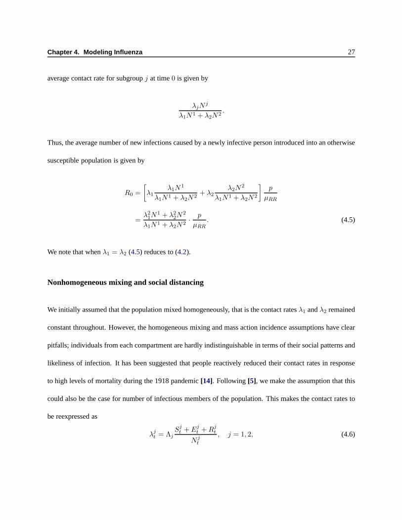
Chapter 4. Modeling Influenza 27
average contact rate for subgroupj at time0 is given by
λjNj
λ1N1 + λ2N2.
Thus, the average number of new infections caused by a newly infective person introduced into an otherwise
susceptible population is given by
R0 =
[
λ1λ1N
1
λ1N1 + λ2N2+ λ2
λ2N2
λ1N1 + λ2N2
]
p
µRR
=λ21N
1 + λ22N
2
λ1N1 + λ2N2·
p
µRR. (4.5)
We note that whenλ1 = λ2 (4.5) reduces to (4.2).
Nonhomogeneous mixing and social distancing
We initially assumed that the population mixed homogeneously, that is the contact ratesλ1 andλ2 remained
constant throughout. However, the homogeneous mixing and mass action incidence assumptions have clear
pitfalls; individuals from each compartment are hardly indistinguishable in terms of their social patterns and
likeliness of infection. It has been suggested that people reactively reduced their contact rates in response
to high levels of mortality during the 1918 pandemic[14]. Following [5], we make the assumption that this
could also be the case for number of infectious members of thepopulation. This makes the contact rates to
be reexpressed as
λjt = Λj
Sjt + Ej
t +Rjt
N jt
, j = 1, 2, (4.6)

Chapter 4. Modeling Influenza 28
whereΛj are fixed constants,j = 1, 2. Using this definition,λjt decreases whenever there is a high number
of infectious agents in the population. As mentioned in[5], other functional forms are possible; we rely on
(4.6) because it provides a simple way to capture changes in contact rates as a function of severity of the
epidemic.
Additionally, we also consider a scenario in which authorities impose social distancing measures as soon
as the epidemic is declared. This kind of public health intervention was used in some cities of the United
States during the 1918 epidemic with different degrees of success. San Francisco, St. Louis, Milwaukee, and
Kansas had the most effective social distancing bans, reducing transmission rates by up to 30 - 50%[14]. A
similar situation took place in Mexico during the last 2009 H1N1 epidemic, where venues such as schools,
movie theaters, and restaurants were forced to close temporarily. It is estimated that the transmission of the
disease was diminished by29% to 37% [19]. We incorporate this element by multiplying the contact rates
by an additional dampening factor when the epidemic is considered declared and until the rate of growth of
daily infectives is below some threshold (we refer the reader to section3.2). Effectively, the contact rate for
groupj at timet becomesλjt = θΛj
(
Sjt+E
jt+R
jt
Njt
)
(0 < θ < 1) when the epidemic is officially ongoing;
otherwise, it remains as per equation (4.6).
4.3 Robustness in planning
In planning the response to a future or impending epidemic, one would need to rely at least partly on an
epidemiological model, and such a model would have to undergo careful calibration in order to be put to
practical use. This is especially the case for the SEIR modelpresented above, which is rich in parameters that
need to be estimated to fully define the trajectory of the epidemic. In the case of a flu pandemic caused by an
unknown virus strain, new parameter values would need to be promptly estimated as the epidemic emerges.

Chapter 4. Modeling Influenza 29
Ideally, robust statistical inference would provide information on all parameters, though data paucity would
present a challenge.
On the positive side, the infectious and incubation periodscan usually be independently estimated via clini-
cal monitoring of infected agents, either by observation oftransmission events or by the use of more detailed
techniques[42].
On the other hand, it is not clear how to accurately estimate the transmission rateλjp. One approach is to
approximate the basic reproductive ratioR0 and the mean infectious period, and then use equation (4.2).
There are multiple ways of estimatingR0; see, for example,[20]. Given that the definition ofR0 is based
on the early stages of the epidemic, one should examine its early behavior. However, the progression of
the epidemic in its initial stages could fluctuate widely because of the very small number of initial cases,
making the fitting process more difficult[42].
Direct estimation of the transmission rate gives rise to a number of challenges[79, 83]. First, pandemic
influenza (along with smallpox and pneumonic plague) has notbeen present in modern times frequently
enough so as to gather sufficient data for accurate estimation. Second, for existing age-specific transmission
models, there are more parameters than observations on riskof infection for each age class. The infectivity
of the disease can be approximated using serologic data and contact rates are usually estimated from census
and transportation data after making assumptions about thecontact processes that reduce the number of
unknowns to the number of age classes. However, both contactor infection rates estimates can serve only
as a baseline; a population could change its behavior significantly during a severe epidemic (due to school
closures, for example); further, environmental changes (e.g. weather changes) could also have a significant
impact on the virus transmissibility[52].
The infectivity parameterp is particularly hard to estimate because (at least partly) it reflects the character-
Chapter 4. Modeling Influenza 30
istics of the virus; it is usually estimated after the epidemic has taken place. It is very difficult to predict
the evolution of new virus strains. In fact, as far as we know[67, 56] research that relates mutations of
influenza virus to infectivity is inconclusive. Previous work has proposed different upper and lower bound
values forp, depending, among other factors, on the geographical location of the study and the pandemic
wave of interest. For example, Walling et al. use the interval [0.025, 0.5] in one work[79] and[0.02, 0.16]
in another[80]. Both studies use these intervals to conduct sensitivity analysis. In another study, Larson
[47] classifies the population into three groups according to social activity levels; the three groups havep
value0.07, 0.09 and0.12 and correspondingλ values50, 10 and2, respectively. In summary, the precise
estimation ofp values appears quite challenging, especially prior to or even during an epidemic.
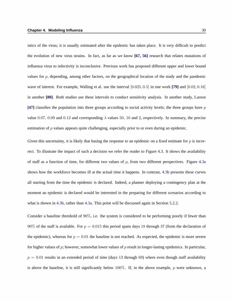
Given this uncertainty, it is likely that basing the response to an epidemic on a fixed estimate forp is incor-
rect. To illustrate the impact of such a decision we refer thereader to Figure4.3. It shows the availability
of staff as a function of time, for different two values ofp, from two different perspectives. Figure4.3a
shows how the workforce becomes ill at the actual time it happens. In contrast,4.3bpresents these curves
all starting from the time the epidemic is declared. Indeed,a planner deploying a contingency plan at the
moment an epidemic is declared would be interested in the preparing for different scenarios according to
what is shown in4.3b, rather than4.3a. This point will be discussed again in Section5.2.2.
Consider a baseline threshold of90%, i.e. the system is considered to be performing poorly if fewer than
90% of the staff is available. Forp = 0.015 this period spans days18 through37 (from the declaration of
the epidemic), whereas forp = 0.01 the baseline is not reached. As expected, the epidemic is more severe
for higher values ofp; however, somewhat lower values ofp result in longer-lasting epidemics. In particular,
p = 0.01 results in an extended period of time (days13 through69) where even though staff availability
is above the baseline, it is still significantly below100%. If, in the above example,p were unknown, a

Chapter 4. Modeling Influenza 31
80%
85%
90%
95%
100%
% A
vailable
Work
forc
e
75%
1
11
21
31
41
51
61
71
81
91
101
111
121
131
141
151
161
171
181
191
201
211
221
231
241
251
261
271
281
291
Time
p = 0.01 p = 0.015 Starting day of epidemic
(a) An absolute perspective in time: Curves start from the moment infectives areintroduced into the susceptible population.
80%
85%
90%
95%
100%
% A
vailable
Work
forc
e
75%
1 6
11
16
21
26
31
36
41
46
51
56
61
66
71
76
81
86
91
96
101
106
111
116
121
126
131
136
141
146
Time (from declaration of epidemic)
p = 0.01 p = 0.015
(b) A planner’s perspective: Curves forboth epidemicsstart from the moment anepidemic is declared.
Figure 4.3: Availability of workforce as epidemic progresses for different values ofp.
planner would have to carefully ration scarce resources over a nearly month-long period. If the planner were
to assume afixedvalue forp throughout the epidemic, then the example suggests allocating comparatively
higher levels of surge staff to earlier periods of time, to overcome the higher shortfalls to be expected in the
case of higher values forp. Of course, this higher level of initial allocation needs tobe carefully chosen to
obtain maximum reward.

Chapter 4. Modeling Influenza 32
Consider now Figure4.4, which shows the impact of achangein p in the midst of an epidemic. Here,
p changes from0.012 to 0.03 on day130, 28 days after the epidemic has been declared. Thus, for more
than half of the epidemic, the disease spreads slowly and even though the90% baseline is approached, it is
not reached. However, after the change inp the epidemic becomes severe and a significant shortfall arises.
This type of variability would be especially problematic when resources are limited. The epidemic, on the
basis of observations of its initial progression, would likely be classified as relatively mild, and, perhaps,
action might be taken to at least partially abandon the surgestaff buildup. However, if the a change inp as
shown in Figure4.4were plausible, then a careful planner would have to hedge byholding back staff so as
to handle the potentially critical situation in later periods. Should the change inp not take place, the chart
indicates that any held back staff would essentially be wasted. And should the change take place somewhat
earlier, then the opportunity cost is significantly higher.The critical question, of course, is whether this
type of virus behavior is possible. As far as we can tell, current knowledge of the influenza virus cannot
categorically reject a change inp as shown, although planning for such a change might be construed as an
overly conservative action. Thus, it remains to be seen if a robust strategy that can protect against a change
in p entails higher cost or other compromises.
In this paper we model the variability of the productλjp using techniques derived from robust optimization.
For ease of exposition, we assume that the infectivity probability p is uncertain, and that the values for
the contact ratesλj are fixed (and known); thus the contact probabilitiesβt are also fixed. Our algorithm’s
flexibility would allow us to easily incorporate uncertainty in other parameters; however, as explained above,
we advocate that the biggest source of uncertainty relies onthe contagion rate. Our goal is to produce
surge staff deployment strategies that are robust with respect to variability ofp in a number of models
of uncertainty. Robust optimization provides an agnostic methodology for assessing competing allocation
plans and for computing good plans according to various criteria. Above, we described two such criteria.

Chapter 4. Modeling Influenza 33
0.75
0.8
0.85
0.9
0.95
1
% A
vailab
le w
ork
forc
e
0.7
1
13
25
37
49
61
73
85
97
109
121
133
145
157
169
181
193
205
217
229
241
253
265
277
289
Time
changing p p = 0.012 p = 0.03 Epidemic is declared
(a) An absolute perspective in time: Curves start from the moment infectives areintroduced into the susceptible population.
0.75
0.8
0.85
0.9
0.95
1
% A
vailab
le w
ork
forc
e
0.7
1 7
13
19
25
31
37
43
49
55
61
67
73
79
85
91
97
103
109
115
121
127
133
139
145
%
Time (from declaration of epidemic)
changing p p = 0.012 p = 0.03
(b) A planner’s perspective: Curves forall three epidemicsstart from the moment anepidemic is declared.
Figure 4.4: Availability of workforce as epidemic progresses when probability of contagionp is allowed to changeduring theepidemic.
Our optimization procedures make it possible to efficientlyevaluate multiple plans and different levels of
conservatism.

Chapter 5. Robust Models 34
55Robust Models
5.1 Performance Measures
Personnel shortage during an epidemic may jeopardize the continuity of operations of critical infrastructure
organizations. To gauge the impact of this shortfall, we consider cost functions that model two scenarios. In
the first one the organization requires at least certain percentage of personnel present to operate. This could
be the case of water and energy plants, as mentioned in[39]. The second scenario uses classic queueing
theory to measure the simultaneous impact of the decrease innumber of available workers and the change
in demand for the service that the organization provides. Health care institutions would be clear examples
in this context.

Chapter 5. Robust Models 35
5.1.1 Threshold functions
Here we model an organization that requires a minimum numberof staff in order to operate under normal
conditions. We further assume that this “minimum” is asoftconstraint in the sense that if the available staff
should fall below the threshold, the organization will still manage to operate, but at very large cost. This
could be the case, for example, if the organization is able topurchase output or hire staff from another source
(such as a competitor) or if it is able to reduce its level of service or output, at cost.
To model this behavior, we assume that operating costs at each point in time are given by a convex piecewise
linear function. This function is represented as the maximum of L linear functions, with slopesσL <
σL−1 < . . . < . . . σ1 = 0 and interceptskL > kL−1 > . . . > k1 = 0. Thus, denoting byωt the work force
level at timet andzt the cost associated with time periodt, we have
zt = max1≤i≤L
{σi ωt + ki} . (5.1)
5.1.2 Queueing models
We are interested in modeling basic queueing systems where both the service rate and the incoming demand
rate are affected by the evolution of the epidemic. For each time periodt, denote the average incoming
demand rate byζt and letst denote the number of available servers (staff). The system utilization at timet,
using an M/M/st queueing model, is given by
ρt =ζtstµ
. (5.2)

Chapter 5. Robust Models 36
As it is well known,ρt and related quantities are good indicators of system performance. In our simulations
of severe epidemics,ρt can grow larger than1, a situation that depicts a system that is catastrophicallysat-
urated (a situation observed during 2010’s H1N1 pandemic[73, 27]) and consequently system performance
will drastically suffer. Accordingly, we choose as a reasonable representative of “cost” incurred at timet
an exponentially increasing function ofρt. In particular we considereρt−δ (for small δ > 0) which we
approximate with a piecewise-linear function, much as in Section 5.1.1. Other alternatives are possible. For
example, one could use a traditional measure of system performance, such as average queue length for an
M/M/st system, computed using a shiftedρt, i.e. a quantityρt = ρt − δ for appropriateδ.
In a regime whereρt is close to (but smaller than)1, one could use one of the popular measures of queueing
system performance as “cost” – or useρt itself as the cost.
5.1.3 Other cost functions
Other situations of practical relevance besides the two considered above are likely to arise. Our robust
planning methodology, described below, is flexible and rapid enough that many alternate models could be
accommodated. Moreover, we would argue that in the context of the cost associated with staff shortfall, any
reasonable cost function would be, broadly speaking, increasing as a function of the shortfall. The approach
described above approximates cost, in the two cases we listed, using piecewise-linear convex functions, and
we postulate that many cost functions of practical relevance can be successfully approximated this way.
5.2 Robust Models
We now describe our methodology for the robust surge staffingproblem. We will first describe our uncer-
tainty model, then the deployment policies we consider, andfinally the robust optimization model itself.

Chapter 5. Robust Models 37
In what follows, we make the assumption that the total quantity of surge staff is small enough that their
deployment does not affect the evolution of the epidemic in the SEIR model, in particular the valuesβt.
5.2.1 Uncertainty models
Let pt denote the probability of contagion at timet (time measured relative to the declaration of the epi-
demic). The model for uncertainty inp that we consider embodies the notion of increasing uncertainty in
later stages of the epidemic. We will first describe the modeland then justify its structure. We assume that
there are four given parameterspL, pU , pL, andpU . The model behaves as follows:
There is a time periodt, unknown to the planner, such that for1 ≤ t ≤ t, pt assumes a constant (but
unknown to the planner) value in[pL, pU ], and fort < t, pt assumes a constant (and also unknown to the
planner) value in[pL, pU ].
We stress thatt is not known to the planner. We are interested in cases wherepL ≤ pL andpU ≤ pU , that
is to say, the period following dayt exhibits more uncertainty than the initial period. We can justify our
model as follows. In the event of an epidemic, a planner wouldbe able to obtain some information on the
spread of the epidemic in the period leading to the actual declaration of the epidemic, resulting in a (perhaps
tight) range of values[pL, pU ]. As we will discuss below (Section5.2.2) we are interested in surge staff
deployment strategies with limited flexibility, i.e. requiring staff commitment levels that are prearranged.
In this setting, at the point when the epidemic is declared, the planner would deploy a staff deployment
strategy. A prudent planner, however, would not simply accept the range[pL, pU ] as fixed. In particular,
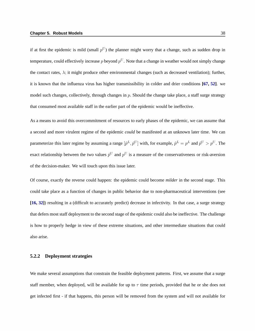
Chapter 5. Robust Models 38
if at first the epidemic is mild (smallpU ) the planner might worry that a change, such as sudden drop in
temperature, could effectively increasep beyondpU . Note that a change in weather would not simply change
the contact rates,λ; it might produce other environmental changes (such as decreased ventilation); further,
it is known that the influenza virus has higher transmissibility in colder and drier conditions[67, 52]. we
model such changes, collectively, through changes inp. Should the change take place, a staff surge strategy
that consumed most available staff in the earlier part of theepidemic would be ineffective.
As a means to avoid this overcommitment of resources to earlyphases of the epidemic, we can assume that
a second and more virulent regime of the epidemiccould be manifested at an unknown later time. We can
parameterize this later regime by assuming a range[pL, pU ] with, for example,pL = pL andpU > pU . The
exact relationship between the two valuespU andpU is a measure of the conservativeness or risk-aversion
of the decision-maker. We will touch upon this issue later.
Of course, exactly the reverse could happen: the epidemic could becomemilder in the second stage. This
could take place as a function of changes in public behavior due to non-pharmaceutical interventions (see
[16, 32]) resulting in a (difficult to accurately predict) decrease in infectivity. In that case, a surge strategy
that defers most staff deployment to the second stage of the epidemic could also be ineffective. The challenge
is how to properly hedge in view of these extreme situations,and other intermediate situations that could
also arise.
5.2.2 Deployment strategies
We make several assumptions that constrain the feasible deployment patterns. First, we assume that a surge
staff member, when deployed, will be available for up toτ time periods, provided that he or she does not
get infected first - if that happens, this person will be removed from the system and will not available for

Chapter 5. Robust Models 39
deployment in the future. We also assume that the pool of available surge staff over the planning horizon is
finite. Finally, there is a maximum quantity of surge staff that can be summoned on any given time period.
More detailed models are possible and easy to incorporate inour optimization framework.
In this paper we will focus onoff-line, or fixed strategies. More precisely, we assume that adeployment
vector is computed immediately after an epidemic is declared, on the basis of the available information.
From a formal perspective, the deployment vector is obtained as follows:
(1) First, the epidemic must be declared. As indicated in Section 3.2, this takes place as soon as the
percentage of infected individuals exceeds some (small) threshold.
(2) Based on data available at that point, estimates are constructed for the various SEIR parameters. In
particular, the ranges[pL, pU ] and[pL, pU ] for p (see Section5.2.1) are constructed.
(3) Using as inputs the population statistics, the cost function, the nominal SEIR model parameters, and
the uncertainty model forp, we compute the deployment vectorh = [h1, h2, . . . , hT ], whereht
indicates the number of staff procuredt time periodsafter the declaration of the epidemic. The
parameterT is chosen large enough to encompass one epidemic wave and will be discussed later.
We next address some points implicit in (1)-(3). First, recall that in the SEIR framework the formal epidemic
will have a starting point which precedes the time period when an epidemic is actually declared. The exact
magnitude of this run-up period isnotknown to a decision maker. In all our notation below (as in (2)above),
“time period 1” refers to the time period where the epidemic was declared, that is to say, we always label
time periods by the amount elapsed since the declaration of the epidemic. When using the SEIR machinery
to simulatean epidemic, of course, we always proceed as in the formal model, and we merely relabel as
“time = 1” that period where the declaration condition is first reached (since that would be the start of the

Chapter 5. Robust Models 40
epidemic as far as a planner is concerned).
Also, we assume that the epidemic iscorrectly declared, that is to say, the first day in which the criterion
in Section3.2applies is correctly observed. In practice, this observation would include noise (for example,
due to individuals infected by a different strain) but we make the assumption that the resulting decrease in
strategy robustness is small.
Item (2), the estimation of the SEIR model and in particular the construction of the initial range[pL, pU ],
gives rise to a host of other issues that are outside the scopeof this paper (but are nonetheless important).
We assume that at the time the epidemic is declared there is enough data (however incomplete, and noisy)
to enable the application ofrobust least squares methods (see e.g.[25]) to fit an SEIR model, and that the
model is sufficiently accurate to permit point estimates forall parameters other thanp. Having constructed
the initial range[pL, pU ], the later range[pL, pU ] is constructed on the basis of (a) risk aversion, and (b)
environmental considerations. The role of (a) is clear -forexample, we could obtainpU by adding topU a
multiple (or fraction) of the standard deviation ofp in the observed data. As an example for (b), an epidemic
that starts in late-Autumn might possibly become more infectious as colder weather develops.
Another point concerns the time horizon,T , for the SEIR model (see Section??) which to remind the reader
is measured from the point that the epidemic is declared. It is assumed thatT is large enough to handle an
epidemic of interest. If we assume a fixed (but unknown)p, then the milder (i.e., less infective) epidemics
will tend to run longer, but, significantly, will also be lessdisruptive. Higher values ofp give rise to sharper
epidemics in the near term. From a technical standpoint, theparameterspL andpL can be used to construct
estimates forT . In order to be sure that we capture as much of an epidemic as possible, in this study we will
use values forT up to 150, which according to our experiments seems more thanadequate.
One could consider models of epidemics spanning, for example, a one-year period, with multiple epidemic

Chapter 5. Robust Models 41
“waves”. If some of these waves are very prolonged then they will necessarily be mild waves for long pe-
riods of time. As a result, during such long, mild epidemic periods (1) the social cost will be low, and (2)
a significant pool of the population will become sick and as a result become immune to the virus. Conse-
quently, future epidemic waves will necessarily be milder and cause decreased social cost (so surge staff
will be less critical). On the other hand, over a long period we could have well-separated strong epidemic
waves1. However, we would argue that from the perspective of surge staff deployment, each such wave
should be handled as a separate event, with its own surge staff deployment strategy.
A significant element in our approach is that it produces a fixed deployment vectorh1, . . . , hT which, from
a formal standpoint, will be applied regardless of observedconditions. Of course, the strategy should be
interpreted as a template and a planner would apply small deviations from the planned surge levels, as
needed. In any case, we have focused on this assumption for practical reasons. Having a pre-arranged
schedule greatly simplifies the logistics of deploying possibly large numbers of staff, especially if many of
the staff originate from geographically distant sources.
A broader class of models would allow for on-the-fly revisionof a strategy in the midst of an epidemic,
which would allow a planner to dynamically react to changes in the epidemic.
However, a significant underlying issue concerns the actualflexibility that would be possible under a virulent
epidemic. We expect that large, sudden changes in deployment plans may be difficult to implement. In
particular, if a significant and unplannedincreasein surge staff is needed, it may prove impossible to rapidly
attain this increase; and by the time the surge staff is available a severe peak of the epidemic may already
have taken place. See Section6.1.3for some experimental validation of these views.
1This was the case of H1N1: the first wave hit in the spring into the summer, followed by another outbreak in the fall, both of2009.

Chapter 5. Robust Models 42
A different type of dynamic strategy would implement many, but small corrections as conditions change.
We will discuss examples of such strategies (and appropriate modifications to our methodology) in Section
8; an issue in this context is the calibration of our statement“as conditions change” in an environment that
will be characterized by noisy, partial and late data.
Last, but not least, while implicitly assumed in our description of theSEIR model, we reiterate that we
consider that the deployment of surge staff does not alter the course of the epidemic. We assume that the
number of additional workers is too small to change significantly the social contact patterns during the
epidemic. Additionally, in the case of hospitals or clinicswe take the position that surge staff is brought
in to preserve operations continuity as much as possible, but they do not have any direct incidence on the
outcome of patients infected with the flu. This is mainly because it is not clear whether existing medications
would be effective with a new virus strain - proper vaccines are not likely to be ready for a pandemic. If
antiviral medications were available, they are usually expensive and should be carefully administered for
it to be the most effective. Recommendations point towards focusing on the treatment of ill health care
workers, and not the general population[21, 50, 61]. A model for the potential impact of these medications
- such as a decrease in the infectious or recovery rates - would be needed and is considered as a possible
refinement to this work.
5.2.3 Robust problem
We can now formally state the problem of computing an optimalrobust pre-planned staff deployment
strategy. Leth denote a deployment vector andH, the set of allowable deployment vectors. Let~p =

Chapter 5. Robust Models 43
(p1, p2, . . . , pT ) be a vector indicating a value ofp for each time period. Define
V (h | ~p) := cost incurred by deployment vectorh, if the infection probability equalspt at timet. (5.3)
[Here we remind the reader that time is measured relative to the declaration of the epidemic.] LetP indicate
a set of vectors~p of interest; our uncertainty set. Our robust problem can nowbe formally stated, as follows:
Robust Optimization Problem
V ∗ := minh∈H
max~p∈P
V (h | ~p). (5.4)
Problem (5.4) explicitly embodies the adversarial nature of our model. Given a choice of vectorh, a fictitious
adversary chooses that realization of the problem data (thecontagion probabilities) that maximizes the
ensuing cost; the task for a planner is to minimize this worst-case cost. The setH describes how staff
deployment plans are constrained. In our implementations and testing, we assume that any deployed staff
person works for a given numberτ of time periods, or until he or she gets sick; following this period of
service this person will not be available for re-deployment. We also assume that whenever surge-staff is
called up, there is a one-period lag before actual deployment (this assumption is easily modified to handle
other time lags).
Finally, we model the impact of the epidemic on surge staff using the SEIR model with parameters as for
the workforce group (λ2t andµE2
), and we assume that the total quantity of available surge staff is small
enough so as to not modify the outcome of the epidemic.
In Chapter7 we will present an efficient procedure, based on linear programming, for solving problem (5.4)
to very tight numerical tolerance.

Chapter 6. Numerical Experiments 44
66Numerical Experiments
In this chapter we investigate the structure of the optimal robust policies by numerical experiments. First,
it is worth raising a point concerning “approximate” vs “exact” solutions. Our algorithms construct nu-
merically optimal solutions to the formal problems they solve; nevertheless, as argued above, our models
approximate real problems. Again, we postulate that given the context (i.e. the behavior of social enti-
ties) an approximation is the best we can hope for; moreover we expect that robust strategies computed for
the approximate models will translate into actual robustness in practice. This last feature can at least be
experimentally tested through simulation, as we present via examples in this section.
In order to assign numerical values to the various parameters in our models, we followed the existing lit-
erature and consulted with various experts[67, 56]. The numbers in the literature may vary significantly
depending on various factors such as the location where the study took place, the underlying model for
which the parameters were calibrated, and the epidemic waveof study. For example, published values for

Chapter 6. Numerical Experiments 45
the influenzaR0, the number of secondary transmissions caused by an infected individual in a susceptible
population, range from1.68 to 20 [53]. Our main sources are listed in Table6.1.
6.1 Examples in a health care setting
We now present examples modeling a hospital of the size of NewYork-Presbyterian Hospital in New York
City under slightly different scenarios. Staff at this hospital amounted to19, 376 in 2010 (we have rounded
this up to20, 000) and served a population of approximately900, 000 people[59]. We used these numbers
as a baseline to obtain different scenarios with different initial conditions.
In the event of an epidemic, hospitals will be likely to experiment surge demand trailing the incidence curve.
We use the queueing-based cost function to capture both shifts in demand and workforce availability while
the epidemic ensues. This increase in demand for service is modeled by adding a proportional factor ofI1t
to the average arrival rate of patients when we compute the system’s occupation rate,ρt:
ρt =ζ + δ I1tstµ
. (6.1)
6.1.1 Example 1
For this example we assume 3,000 surge staff members are available, each of which will be called up for at
most one period of service lasting one week. If the member becomes infectious while on call, then service
is terminated with no further future availability.
We used the uncertainty model in Section5.2.1which allowspt to change once. The change is further
constrained to take place within a fixed range of time periods.

Chapter 6. Numerical Experiments 46
Table 6.1: List of references for different parameter values.
Parameter Description Value(s) Reference
Epidemic related parameters
p Probability of contagion [0.02, 0.16]a [80]{0.07, 0.09, 0.12}b [47]
λ Contact rate 47.48 (per day) [79]35 (per day)c [47]
µ−1
E Latent period 1 day [36]1.9 daysd [50]1.25 days [28]
1.48± 0.48 days [28] and withinµ−1
R Infectious period 2 days [36]4.1 days [50, 49]4.1 dayse [49]
1− f Mortality rate 0.02 [50]0.002 per dayf [28]
1.2%g [19]0.05g [49]
R0 R0 1.68 to 20h [53] and within1.73i [79]2.5j [49]
Length of pandemic wave 8− 12 weeks [28]
Hospital related measures
ζ Patient arrival rate 2,800 ILI cases/dayk [49]µ Service rate 24− 30min/patientl [33]ρ Occupancy rate Average of85%m [22]δ Increase in demand for health care up to50% [58]
Miscellaneous
Seasonal threshold [0.06, 0.076] weeklyn [26]Epidemic threshold [0.064, 0.08] weeklyn [26]
ILI National Baseline 2.4% weeklyo [26]θ Transmission reduction factor 29% to37%p [19]
a 1957 wave in the Netherlandsb Values ofp for different socially active groupsc Weighted average of different age groups presented in the paperd 1957 pandemic wavee Untreated symptomaticf Treated symptomaticg Overall ILI case-fatality ratio during 2009 H1N1 pandemic in Mexicog Spanish Flu fatality rateh From multiple studiesi 1957 wavej Min 1.5, Max 6k Data for Singapore, 2005. Population then was about 4.35 million peoplel Emergency Department, New York Presbyterian Hospitalm Maintained beds capacity for New Jersey Hospitals, 2005n The threshold is for percentage of deaths caused by pneumonia and influenza.It is different for each week throughout the year.o Percentage of influenza-like illness (ILI) patient visits reported through the U.S. Outpatient ILI Surveillance Network.p Estimated effect of social distancing measures during H1N1epidemic in Mexico, 2009

Chapter 6. Numerical Experiments 47
The social contact model assumed the nonhomogeneous-mixing rule described in section4.2. Additionally,
we assumed that social contact rates were dampened by a factor of 30% while the epidemic is declared;
that is, during the days in which the growth of infectives is higher than a given threshold. Additionally, we
assumed an epidemic is declared only once. In other words, once the rate of infectives slow down below the
epidemic threshold, the epidemic is considered to be terminated.
The parameter values for this example are summarized in Table6.2; the range of days wherep is allowed to
change are measured from thestart of the epidemic (rather than the day the epidemic is declared).
Table 6.2: Parameter values for example 1
Parameter Description Value(s)
Epidemic related parametersP Uncertainty set [0.01, 0.012] × [0.0125, 0.0135]
Possible days of change {140, . . . , 160}(Λ1,Λ2) Contact rates (30, 35) per dayµ−1E Latent period 1.9 days
µ−1R Infectious period 4.1 days
1− f Mortality rate 0R0 R0 [1.24, 1.48]
Deployment threshold 2.4% weekly
Population parametersN1 General population size 900,000N2 High risk population size 20,000
[I1, I2] Initial infectives [5,0]
System Utilization (Queueing setting)ζ Patient arrival rate 500 per dayµ Service rate per person 30 patients per dayρ0 Initial occupation rate 0.875δ Daily increase in demand for health care 0.07%
Deployment parametersTotal number of available volunteers 3, 000
τ Length of stay (w/o sickness) 7Deployment lag 1
In what follows, the staff deployment plan computed by our algorithm will be called theRobust Policy. To
gauge its usefulness, we study its performance under different scenarios, each of which is defined by a tuple
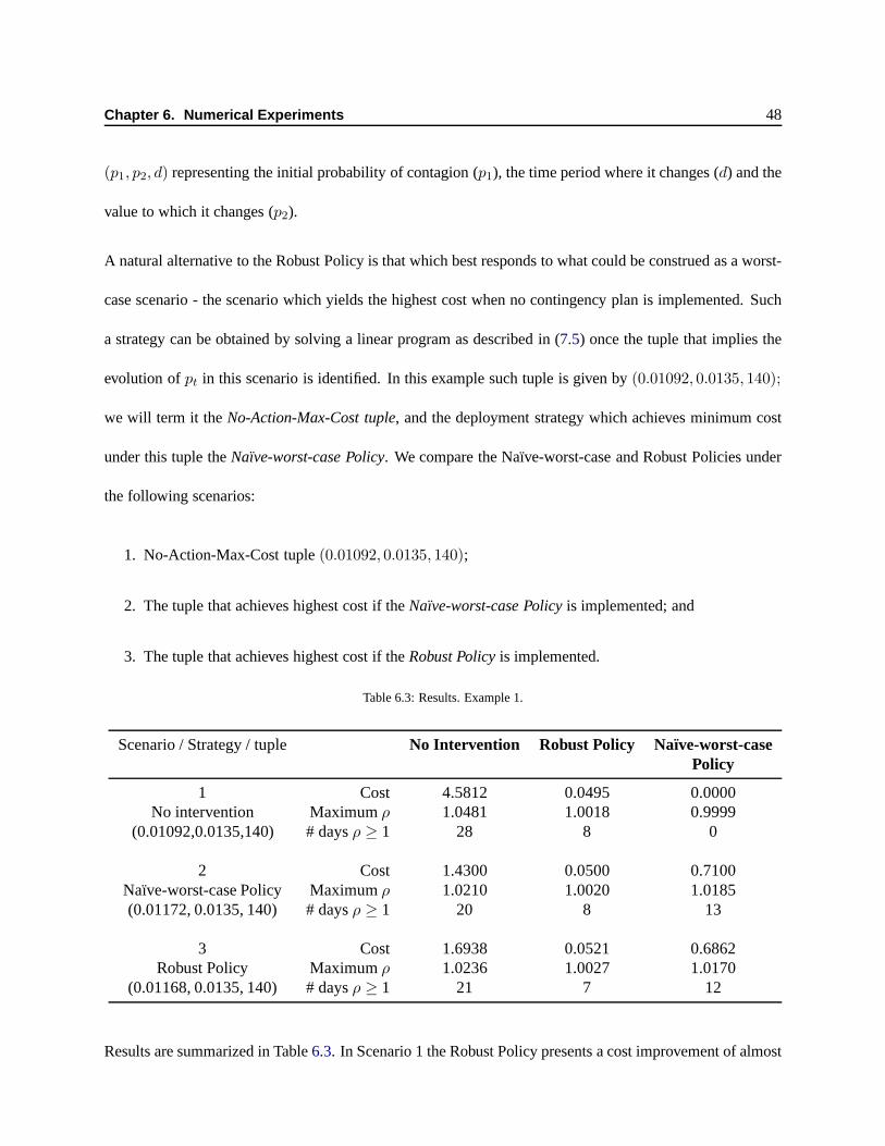
Chapter 6. Numerical Experiments 48
(p1, p2, d) representing the initial probability of contagion (p1), the time period where it changes (d) and the
value to which it changes (p2).
A natural alternative to the Robust Policy is that which bestresponds to what could be construed as a worst-
case scenario - the scenario which yields the highest cost when no contingency plan is implemented. Such
a strategy can be obtained by solving a linear program as described in (7.5) once the tuple that implies the
evolution ofpt in this scenario is identified. In this example such tuple is given by(0.01092, 0.0135, 140);
we will term it theNo-Action-Max-Cost tuple, and the deployment strategy which achieves minimum cost
under this tuple theNaïve-worst-case Policy. We compare the Naïve-worst-case and Robust Policies under
the following scenarios:
1. No-Action-Max-Cost tuple(0.01092, 0.0135, 140);
2. The tuple that achieves highest cost if theNaïve-worst-case Policyis implemented; and
3. The tuple that achieves highest cost if theRobust Policyis implemented.
Table 6.3: Results. Example 1.
Scenario / Strategy / tuple No Intervention Robust Policy Naïve-worst-casePolicy
1 Cost 4.5812 0.0495 0.0000No intervention Maximumρ 1.0481 1.0018 0.9999
(0.01092,0.0135,140) # daysρ ≥ 1 28 8 0
2 Cost 1.4300 0.0500 0.7100Naïve-worst-case Policy Maximumρ 1.0210 1.0020 1.0185(0.01172, 0.0135, 140) # daysρ ≥ 1 20 8 13
3 Cost 1.6938 0.0521 0.6862Robust Policy Maximumρ 1.0236 1.0027 1.0170
(0.01168, 0.0135, 140) # daysρ ≥ 1 21 7 12
Results are summarized in Table6.3. In Scenario 1 the Robust Policy presents a cost improvementof almost

Chapter 6. Numerical Experiments 49
99% over the no-intervention policy. While it is not completelyable to preventρ from exceeding1, it
reduces the number of critical days from 28 to 8, and the maximum ρ from 1.05 to below1.002. Indeed,
the undesirable instability in which a system is put throughwhenρ > 1 is heavily penalized with the use
of the exponential function in our objective function (see5.1.2). On the other hand, under Scenario 1 the
Naïve-worst-case Policy reduces the cost to0; that is, there is no day in whichρ is greater than1. Without
doubt, it represents a better solution than the Robust Policy for this particular case. This result is expected;
the solution derived from that single linear program isspecializedin this scenario, while the Robust Policy,
having to hedge against other possible bad cases, does not perform as well in this instance.
The situation is considerably different, however, when we look at Scenario 2, which achieves the highest
cost when the Naïve-worst-case Policy is being implemented. In this case, the Robust Policy performs much
better than the Naïve-worst-case Policy: the former reduces the cost of this scenario by96.5%, while the
latter does so by only50%; the Robust Policy reduces the number of critical days from20 to 8 days, while
this number jumps to13 for the Naïve-worst-case Policy. The maximum value ofρ is 1.002 for Robust
Policy and1.018 for scenario 2, compared to1.021 with no intervention. The third scenario presents similar
characteristics; what is worth noticing is that even thoughthis is thehighest-costscenario for the Robust
Policy, its cost is still the same as in Scenario 2.
This fact is further illustrated in Figure6.1, where we compare the behavior ofρt with and without inter-
ventions for the three scenarios, together with the deployment patterns. We note that the Naïve-worst-case
Policy deploys staff around in large, sharp bursts between days27 and52. The Robust Policy deployment,
on the other hand, trailsρ in Scenario 1 in a smoother way by calling in personnel in smaller batches, and
also over a longer period of time:36 days. This shows the importance of Scenario 1 as the costliest case and,
at the same time, how the strategy hedges against scenarios where the epidemic has its peak later (than under

Chapter 6. Numerical Experiments 50
100
200
300
400
500
600
0 8
0.85
0.9
0.95
1
1.05
Pro
cure
ment
Str
ate
gy
0
100
0.75
0.8
1 8
15
22
29
36
43
50
57
64
71
78
85
92
99
106
113
120
127
134
141
148
Time from declaration of epidemic
!(Robust);!Cost!=!0.0495 !(No!Interv);!Cost!=!4.58
* Robust!Policy
(a) Scenario 1:Effectiveness of Robust Policy
100
200
300
400
500
600
0 8
0.85
0.9
0.95
1
1.05
Pro
cure
ment
Str
ate
gy
0
100
0.75
0.8
1 8
15
22
29
36
43
50
57
64
71
78
85
92
99
106
113
120
127
134
141
148
Time from declaration of epidemic
!(Worst"case);!Cost!=!0 !(No!Interv);!Cost!=!4.58
* Naïve"worst"case!Policy
(b) Scenario 1:Effectiveness of Naïve-worst-case Policy
100
200
300
400
500
600
0 8
0.85
0.9
0.95
1
1.05Pro
cure
ment
Str
ate
gy
0
100
0.75
0.8
1 8
15
22
29
36
43
50
57
64
71
78
85
92
99
106
113
120
127
134
141
148
Time from declaration of epidemic
!(Robust);!Cost!=!0.05 !(No!Interv);!Cost!=!1.43
* Robust!Policy
(c) Scenario 2:Effectiveness of Robust Policy
100
200
300
400
500
600
0 8
0.85
0.9
0.95
1
1.05
Pro
cure
ment
Str
ate
gy
0
100
0.75
0.8
1 8
15
22
29
36
43
50
57
64
71
78
85
92
99
106
113
120
127
134
141
148
Time from declaration of epidemic
!(Worst"case);!Cost!=!0.71 !(No!Interv);!Cost!=!1.43
* Naïve"worst"case!Policy
(d) Scenario 2:Effectiveness of Naïve-worst-case Policy
100
200
300
400
500
600
0 8
0.85
0.9
0.95
1
1.05
Pro
cure
ment
Str
ate
gy
0
100
0.75
0.8
1 8
15
22
29
36
43
50
57
64
71
78
85
92
99
106
113
120
127
134
141
148
Time from declaration of epidemic
!(Robust);!Cost!=!0.05 !(No!Interv);!Cost!=!1.43
* Robust!Policy
(e) Scenario 3:Effectiveness of Robust Policy
100
200
300
400
500
600
0 8
0.85
0.9
0.95
1
1.05
Pro
cure
ment
Str
ate
gy
0
100
0.75
0.8
1 8
15
22
29
36
43
50
57
64
71
78
85
92
99
106
113
120
127
134
141
148
Time from declaration of epidemic
!(Worst"case);!Cost!=!0.69 !(No!Interv);!Cost!=!1.43
* Naïve"worst"case!Policy
(f) Scenario 3:Effectiveness of Naïve-worst-case Policy
Figure 6.1: Reduction inρ obtained by the Robust and Naïve-worst-case deployment strategies under three scenarios: 1)Highest-cost scenario given that no policy is implemented,2) Highest-cost scenario given that the Naïve-worst-casePolicy is implemented, and 3) Highest-cost scenario given that the Robust Policy is deployed.

Chapter 6. Numerical Experiments 51
the No-Action-Max-Cost tuple), even if not so aggressively. In particular, the last wave of staff deployed by
the Robust Policy (on days54, 58, and63) could seem somehow wasteful under Scenario 1; however their
utility is displayed under Scenario 2, where the Robust Policy tackles a delayed, weakerρ peak much more
effectively than the Naïve-worst-case Policy. Because an unstable system builds up a queue exponentially
fast, even this small changes inρ could translate in significant difference in the load experienced by the
system.
A similar situation is presented in Scenario 3, as illustrated in both Figure6.1 and Table6.3. The Naïve-
worst-case Policy is not as effective as handling what wouldhave been a milder epidemic, while the Robust
Policy performs consistently well. In fact, this is the scenario with highest cost for the Robust Policy;
nevertheless it manages to significantly outperform the Naïve-worst-case Policy here as well. Indeed, a
feature of the Robust Policy is its near-uniform behavior under all scenarios; this epitomizes the use of the
term ’robust’.
Other strategies such as the Naïve-worst-case Policy, on the other hand, may be very sensitive to changes
in p depending on how they are constructed. In this example we make the case that preparing only for
the highest-cost scenario (under the No-Action Policy) is not necessarily enough to be prepared for other
milder cases: This is critical from the point of view of a decision maker: as seen above, a policy built
only to tackle such case does not allocate enough resources to other time periods in which milder cases
may need them the most. At the same time, being able to cut downthe number of days in which the
organization is completely overloaded should represent considerable economic and operational advantages
for the institution implementing the contingency plan. Oneestimate of the costs saved in a given scenario
could be derived as a function of the area between theρ curves corresponding to the No-Action Policy and
the Robust Policy, wheneverρ > 1.

Chapter 6. Numerical Experiments 52
Smoothing out the solution
An additional restriction on the implementation of the proposed Robust Strategy could be for it to be as
regular as possible. In other words, it could be deemed more desirable to have a contingency plan with
fewer fluctuations in the surge staff calls in terms of its applicability. There are several ways of imposing
these constraints. We chose to incorporate the constraints
ht > 0⇒ ht+1 ≤ (1 + r)ht ∀t, (6.2)
where0 < r < 1 is a given tolerance. These constraints allow the policy to consider more even deployment
blocks, avoiding drastic increases in the number of surge staff called in. It also discourages long sequences
of days in which relatively few people are deployed, for the following days would be very constrained if a
strong increase is needed.
At the same time, it is important to mention that these additional restrictions imply a loss in robustness:
constraining the variability of the hiring policies hinders the structure of the strategy’s best response. The
obvious question is how much of this robustness would be lostto favor an easier implementation.
To answer this question and to illustrate the new policies, we repeated Exercise 1 for 3 values ofr : 0.1, 0.2,
and0.3. The changes in the structure of the deployment strategies can be observed in Figure6.2 and the
change in the highest cost in Table6.4. The loss in robustness is modest, but it would be up to the decision
maker to evaluate the trade off.
Table 6.4: Change in highest cost due to smoothing out solution.
Original r = 0.3 r = 0.2 r = 0.1
Highest cost 0.050767 0.051025 0.051308 0.052327% increase 0.51% 1.07% 3.07%
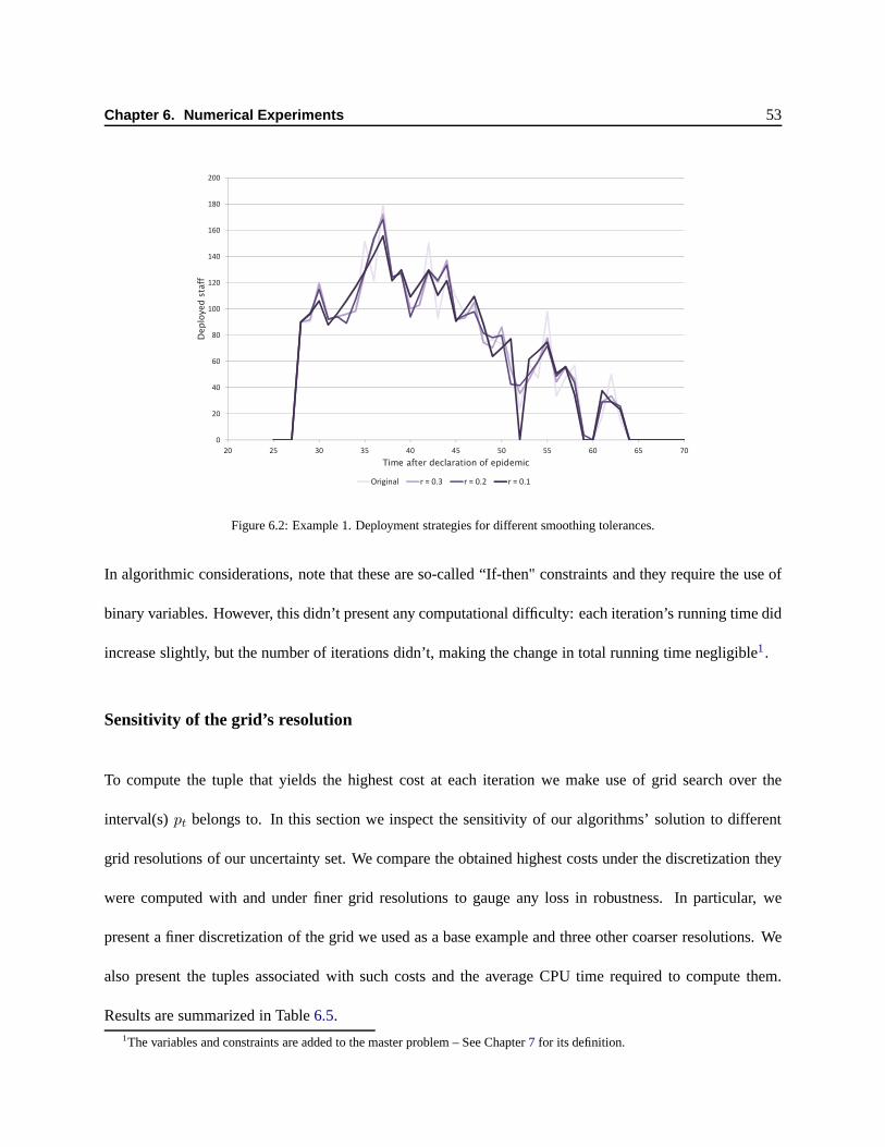
Chapter 6. Numerical Experiments 53
60
80
100
120
140
160
180
200
Deplo
yed s
taff
0
20
40
60
20 25 30 35 40 45 50 55 60 65 70
Time after declaration of epidemic
Original r = 0.3 r = 0.2 r = 0.1
Figure 6.2: Example 1. Deployment strategies for differentsmoothing tolerances.
In algorithmic considerations, note that these are so-called “If-then" constraints and they require the use of
binary variables. However, this didn’t present any computational difficulty: each iteration’s running time did
increase slightly, but the number of iterations didn’t, making the change in total running time negligible1.
Sensitivity of the grid’s resolution
To compute the tuple that yields the highest cost at each iteration we make use of grid search over the
interval(s)pt belongs to. In this section we inspect the sensitivity of ouralgorithms’ solution to different
grid resolutions of our uncertainty set. We compare the obtained highest costs under the discretization they
were computed with and under finer grid resolutions to gauge any loss in robustness. In particular, we
present a finer discretization of the grid we used as a base example and three other coarser resolutions. We
also present the tuples associated with such costs and the average CPU time required to compute them.
Results are summarized in Table6.5.1The variables and constraints are added to the master problem – See Chapter7 for its definition.

Chapter 6. Numerical Experiments 54
This exercise shows the importance of using the correct resolution to compute the final policies. Extremely
fine grids may provide somehow more accurate approximations. At the same time, they can be compu-
tationally much more expensive. Comparing the Base case with the Super Fine case, we can see that the
difference in the highest cost is minimal while the time to find the desired tuple for the finer grid is more
than 30 times more than the time it takes for the Base case grid. As expected, even coarser grid searches
provide faster but less robust solutions. While our algorithm performs well, this analysis suggests that one
could make use of coarse discretizations for the first iterations and finer grids in subsequent iterations.
Table 6.5: Change in highest cost for different discretizations of the uncertainty set. In this example, it is given byP = [0.01, 0.012] × [0.0125, 0.0135] × {140, ..., 160}. Different resolutions were taken for the first 2 intervals.
Discretization cost Highest cost Highest cost Highest cost CPU time Size ofStep1 × Step2 tuple with given resolution with Base resolution with Fine resolution worst-tuple Uncertainty Set
0.00001 x 0.00001 0.050950 - - 125s 420K(Fine) (0.01111,0.0135,140) -
0.00001 x 0.0005 0.050768 - 0.050768 3.75s 16.8K(Base) (0.01172,0.0135,140) (0.01172,0.0135,140)
0.00005 x 0.00005 0.004059 0.2515 0.2515 5.234s 33.6K(Coarse 1) (0.01105,0.0135,156) (0.01172,0.0135,140) (0.01172,0.0135,140)
0.0001 x 0.0001 0.000104 0.3141 0.3141 1.484s 8.4K(Coarse 2) (0.0113,0.0135,140) (0.01172,0.0135,140) (0.01172,0.0135,140)
0.0005 x 0.0005 0.002302 0.2031 0.2031 0.094s 0.336K(Coarse 3) (0.011,0.0135,143) (0.01168,0.0135,140) (0.01168,0.0135,140)
The resulting deployment strategies for the different gridresolutions are also quite dissimilar as shown in
Figure6.3. The deployment strategies resulting from coarser grids are represented in dashed, light-colored
lines, while those obtained from finer discretizations are shown in darker, solid lines. The first thing to
notice is that the differences between the strategies obtained from the Original and the Fine discretizations
are negligible. On the other hand, as the resolution of the grid gets coarser, the staff is deployed in bigger,
more sprawled bursts. The fact that the smoother strategiesare more robust (see Table6.5) shows that, in
this particular example, a more even deployment of the surgestaff is better capable of dealing with different
epidemic scenarios. It is important to mention that this assumes that a certain amount of surge staff is

Chapter 6. Numerical Experiments 55
100
150
200
250
300
350
Deployed
Staff
0
50
100
20 22 24 26 28 30 32 34 36 38 40 42 44 46 48 50 52 54 56 58 60 62 64 66 68 70
Time after declaration of epidemic
Original Super Fine Coarse 1 Coarse 2 Coarse 3
Figure 6.3: Example 1. Deployment strategies for differentdiscretizations of the uncertainty set.
available. We modify this assumption in the following example (Section6.1.2).
Threshold objective function
In this section we present analogous results, now considering a threshold objective function in which cost
increases as staff levels decrease (see5.1.1for more details). For this example we take95% and99% as the
breakpoints of the piecewise linear function: whenever staff levels are below95%, costs increase by 1 unit
for every percentage point workforce availability is reduced; if staff levels are between95% and99% costs
increase by1/4 of a unit for each percentage point, and there is no cost whenever there is99% or more of
the workforce available. In mathematical terms, given a percentage of available staff at timet, ωt ∈ [0, 1],
the daily cost is given by
zt = max{−100ωt + 96,−25ωt + 24.75, 0}. (6.3)
All other parameters remain as listed in Table6.2.
As with the queueing model-based objective, we compare the Robust solution with the Naïve-worst-case

Chapter 6. Numerical Experiments 56
Policy under different scenarios: 1) the No-Action-Max-Cost tuple(0.01092, 0.0135, 140) and 2) the highest-
cost tuple if the Naïve-worst-case Policy is deployed,(0.01168, 0.0135, 140). In this case Scenario 1) coin-
cides with Scenario 3); that is, the tuple that achieves the highest cost if the Robust Policy is implemented
is the same as the No-Action-Max-Cost tuple. As with the queueing model-based objective function, while
the Naïve-worst-case Policy fares better than the Robust Policy in Scenario 1), its cost can be up to28%
higher than the Robust Policy for other tuples. Moreover, given the number of surge staff available, the
Robust Policy avoids going under the preestablished critical threshold of95% in both scenarios, while the
Naïve-worst-case Policy presents as many as8 of these days. These statistics are exhibited in Table6.6.
Table 6.6: Results with threshold function. Example 1.
Scenario / Strategy / No Intervention Robust Policy Naïve-worst-casetuple Policy
1 Cost 83.1445 32.4503 32.2351No intervention & Max. absenteeism 6.90% 4.96% 5.00%
Robust Policy # days AvWF < 95% 28 0 0(0.01092,0.0135,140)
2 Cost 64.3800 29.0090 37.3449Naïve-worst-case Policy Max. absenteeism 5.97% 4.27% 5.95%(0.01168,0.0135,140) # days AvWF < 95% 22 0 8
The structure of the deployment strategies together with its impact on the workforce availability (measured
in percentage) for Scenarios 1 and 2 is displayed in Figure6.4. It is worth nothing that if Scenario 2 took
place, it could be thought that the Robust Strategy is somehow wasteful: staff levels surpass 100% around
day 36 (Figure6.4c). However, one must remember that the strategy must be resilient to all situations,
including one such as Scenario 1, where there is no underutilization of the surge workers (Figure6.4a). In
the same scenario, the Naïve-worst-case strategy not only would deploy too many extra workers (around
day 25) for many more days, it would allow the absenteeism to grow above 5% for8 days as we mentioned
above.

Chapter 6. Numerical Experiments 57
100
200
300
400
500
600
0.92
0.94
0.96
0.98
1
1.02
Pro
cure
ment
Str
ate
gy
% A
vailable
Work
forc
e
00.9
1 8
15
22
29
36
43
50
57
64
71
78
85
92
99
106
113
120
127
134
141
148
Time from declaration of epidemic
%Av WF (Robust)
Cost = 32.4503
%Av WF (No Interv)
Cost = 83.1445
Abs thresh Robust PS
(a) Scenario 1:Effectiveness of Robust Policy
100
200
300
400
500
600
0.92
0.94
0.96
0.98
1
1.02
Pro
cure
ment
Str
ate
gy
% A
vailable
Work
forc
e
00.9
1 8
15
22
29
36
43
50
57
64
71
78
85
92
99
106
113
120
127
134
141
148
Time from declaration of epidemic
%Av WF (Worst!Scen)
Cost = 32.2351
%Av WF (No Interv)
Cost = 83.1445Abs thresh Worst!Scen PS
(b) Scenario 1:Effectiveness of Naïve-worst-case Policy
100
200
300
400
500
600
0.92
0.94
0.96
0.98
1
1.02Pro
cure
ment
Str
ate
gy
% A
vailable
Work
forc
e
00.9
1 8
15
22
29
36
43
50
57
64
71
78
85
92
99
106
113
120
127
134
141
148
Time from declaration of epidemic
%Av WF (Robust)
Cost = 29.009
%Av WF (No Interv)
Cost = 64.38
Abs thresh Robust PS
(c) Scenario 2:Effectiveness of Robust Policy
100
200
300
400
500
600
0.92
0.94
0.96
0.98
1
1.02
Pro
cure
ment
Str
ate
gy
% A
vailable
Work
forc
e
00.9
1 8
15
22
29
36
43
50
57
64
71
78
85
92
99
106
113
120
127
134
141
148
Time from declaration of epidemic%Av WF (Worst!Scen)
Cost = 37.3449
%Av WF (No Interv)
Cost = 64.38Abs thresh Worst!Scen PS
(d) Scenario 2:Effectiveness of Naïve-worst-case Policy
Figure 6.4: Changes in the workforce availability after thedeployment of the Robust and Naïve-worst-case strategies under twoscenarios: 1) Highest- cost scenario given that no policy isimplemented, 2) Highest- cost scenario given that theNaïve-worst-case Policy is implemented.
6.1.2 Example 2
To further illustrate the structure of the Robust Policy under different scenarios, we now consider the pre-
vious example with some modifications. Here, the uncertainty set isp lies in the interval[0.01, 0.0125]
throughout, but can change values once on any day in the range{100, . . . , 115}. R0 is now between 1.24
and 1.54. The total number of available volunteers is2, 000 and the contact rates are not dampened while
the epidemic is being declared. All other data remains as in the first example.
Following the same logic as in the previous example, we present the Robust Policy and compare it to the

Chapter 6. Numerical Experiments 58
Table 6.7: Results. Example 2.
Scenario / Intervention / Tuple No Intervention Robust Policy Naïve-worst-case Policy
1 Cost 3.8332 0.0280 0.0066No intervention Maximumρ 1.0410 1.0012 1.0003
(0.0125, 0.0125, 100) # daysρ ≥ 1 27 10 6
2 Cost 3.5906 0.0280 0.0542Naïve-worst-case Policy Maximumρ 1.0393 1.0019 1.0025(0.01235, 0.0125, 112) # daysρ ≥ 1 26 7 8
3 Cost 3.7320 0.0295 0.0379Robust Policy Maximumρ 1.0403 1.0010 1.0017
(0.01015, 0.0125, 101) # daysρ ≥ 1 26 10 10
140
160
egy
80
100
120
nt
Str
ate
40
60
80
ocure
me
0
20
20 21 22 23 24 25 26 27 28 29 30 31 32 33 34 35 36 37 38 39 40 41 42 43 44 45
Pro
20 21 22 23 24 25 26 27 28 29 30 31 32 33 34 35 36 37 38 39 40 41 42 43 44 45
Time from declaration of the epidemic
Robust Policy Naïve-worst-case Policy
Figure 6.5: Example 2. Structure of the deployment strategies.
Naïve-worst-case Policy (obtained as before by solving thelinear program associated with the highest-cost
tuple of our uncertainty set). We present results for the same three scenarios: the No-Action-Max-Cost tuple,
the costliest tuple for the Naïve-worst-case Policy, and the costliest tuple for the Robust Policy, respectively.
This fact hints on the non-convexity of the problem, a topic we will touch upon later in this section.
Table 6.7 displays the results. The Robust Policy is worse than the Naïve-worst-case Policy in the first
instance, while keeping a fairly consistent and low cost forthe other scenarios; where the Naïve-worst-
case Policy does not perform as well. What is worth noting is that, unlike in the previous example, the

Chapter 6. Numerical Experiments 59
structure of the deployment strategies is much more similar(see Figure6.5); nevertheless, the apparently
small differences make the Robust Policy more resilient to other scenarios. A second observation regards
the structure of the highest-cost tuples evinced by the policies. In this example the No-Action-Max-Cost
tuple corresponds to having an epidemic with afixedprobability of contagionp = 0.0125, the highest in the
interval of the uncertainty set. However, the costliest tuples for the Robust and Naïve-worst-case policies
are quite different.
Cost-benefit analysis
We now present a cost-benefit analysis on the availability ofsurge staff. We took this example as a base
case and recomputed the optimal Robust and the Naïve-worst-case policies assuming1, 000, 1, 500, 2, 500,
and3, 000 surge staff on hand. Table6.8displays their corresponding worst-scenario tuples alongwith the
associated costs for when the corresponding policy is beingimplemented and for when no contingency plan
was put in place.
We point out that the difference in the highest-cost tuples explains the difference in the costs when no
intervention takes place: the highest-cost scenarios are obtained assuming that a corresponding policy is
being implemented. In fact, it is interesting to see how the structure of the tuples change with the different
policies. When there is not much staff available, the worst scenario for both policies is given by the tuple
(0.0125, 0.0125, 100). The highest costs for the Naïve and the Robust Policies are very close, although the
deployment strategies not as much. When there are1, 000 and1, 500 staff available, the Robust Strategies
are more concentrated towards the middle, while the Naïve-worst-case Policies are more spread out (see
Figure6.6).
Table6.8 also presents the change in the maximum value ofρ and the number of days thatρ is at or above

Chapter 6. Numerical Experiments 60
1. The last row of the table shows the ratio between the change in the highest cost and the change in the
number of available surge staff. For example, when there are1, 500 volunteers available, there is a change
in the cost of0.156% for each of the500 that are now not at hand. At the same time, the benefit obtainedper
additional worker available decreases for both the Robust and the Naïve-worst-Case Policy, but more so for
the latter. That is, the Robust Strategies make better use (cost-wise) of extra staff in terms of the highest cost.
This is again because the Robust Policy “knows” how to allocate the additional staff to cover up for different
bad cases, while the Naïve-worst-case Policy has only one scenario to focus on. This fact is particularly
noticeable when the Naïve Policy chooses to hire only2, 579 emergent workers out of the3, 000 that are
available. While this amount of staff is enough to tackle thehighest-cost scenario (under no intervention),
it is not distributed well enough to tackle milder cases, whereas the Robust Policy has a maximum cost of0
when so much staff is on hand.
Figure6.6illustrates the structure of the above mentioned strategies. To make the strategies comparable, we
display the percentage of the staff that is called in on each day; percentages are stacked on top of each other.
The plots further support our claims: for the cases in which the Robust Policy has more surge staff available,
more people are hired towards the end of the planning horizon, while the Naïve-worst-case Policies look to
tackle the system congestion early after the epidemic has been declared.
Non-convexity
As the examples above make clear, the systems we study can be strongly dependent on the choice ofp,
with clear nonlinearities and non-convexities. This justifies the use of robustness in the design of response
strategies.
To further study the dependence onp, we considered the cost of a set of strategies whenp is constant through-

Chapter 6. Numerical Experiments 61
Table 6.8: Cost-Benefit Analysis for different quantities of available surge staff.
Robust Policy
Total staff deployed 1,000 1,500 2,000 2,500 3,000
Highest-cost tuple(p1, p2, d) (0.0125,0.0125,100) (0.0125,0.0125,100) (0.01015,0.0125,101) (-,-,-) (-,-,-)
Highest cost 1.755971 0.818334 0.029545 0 0
Highest cost (No Int) 3.8332 3.8332 3.732 3.8332 3.8332
Maximumρ 1.02 1.02 1.001 0.999 0.998
Maximumρ (No Int) 1.04 1.04 1.04 1.04 1.04
# daysρ ≥ 1 27 27 10 0 0
# daysρ ≥ 1 (No Int) 27 27 26 27 27
Cost Change / Extra Surge Staff 0.345% 0.158% - -0.006% -0.003%
Naïve-worst-case Policy
Total staff deployed 1,000 1,500 2,000 2,500 2,579
Highest-cost tuple (0.0125,0.0125,100) (0.0125,0.0125,100) (0.01235,0.0125,112) (0.01235,0.0125,105) (0.01235,0.0125,113)
Highest cost 1.75351 0.811355 0.05418 0.018956 0.015555
Highest cost (No Int) 3.8332 3.8332 3.6077 3.6997 3.5906
Maximumρ 1.02 1.01 1.002 1.002 1.002
Maximumρ (No Int) 1.04 1.04 1.04 1.04 1.04
# daysρ ≥ 1 27 27 8 3 2
# daysρ ≥ 1 (No Int) 27 27 26 26 26
Cost Change / Extra Surge Staff 0.345% 0.156% - -0.002% -0.002%
20%
30%
40%
50%
60%
f sta
ff a
llocate
d
0%
10%
15 16 17 18 19 20 21 22 23 24 25 26 27 28 29 30 31 32 33 34 35 36 37 38 39 40 41 42 43 44 45
% o
f
Time from declaration of epidemicTH = 1000 TH = 1500 TH = 2000 TH = 2500 TH = 3000
(a) Robust Policies.
20%
30%
40%
50%
60%
f sta
ff a
llocate
d
0%
10%
15 16 17 18 19 20 21 22 23 24 25 26 27 28 29 30 31 32 33 34 35 36 37 38 39 40 41 42 43 44 45
% o
f
Time from declaration of the epidemicTH = 1000 TH = 1500 TH = 2000 TH = 2500 TH = 2579
(b) Naïve-worst-case Policies.
Figure 6.6: Changes in the distribution of the deployment strategies for different amounts of available surge staff.

Chapter 6. Numerical Experiments 62
1
1.5
2
2.5
3
3.5
4
cost
0
0.5
0.0
1145
0.0
1155
0.0
1165
0.0
1175
0.0
1185
0.0
1195
0.0
1205
0.0
1215
0.0
1225
0.0
1235
0.0
1245
probability of contagion
(a) Total cost as a function ofp under no intervention.
0.01
0.015
0.02
0.025
0.03
0.035
cost
0
0.005
0.0
1235
0.0
1237
0.0
1239
0.0
1241
0.0
1243
0.0
1245
0.0
1247
0.0
1249
probability of contagion
(b) Total cost as a function ofp under 3 different strategies.
Figure 6.7: Total cost of an epidemic as a function ofp under a)No intervention, and b) Three different deploymentpolicies.
out the epidemic. Figure6.7aplots the objective function as a function ofp in the interval[0.0115, 0.0125]
when there is no intervention; clearly it is monotone increasing inp. Figure6.7b, on the other hand, shows
the cost of three strategies for computed by our algorithms2. These curves are certainly not monotonic and,
not surprisingly, particular values ofp are able to exploit relative “gaps” in deployment. This facthas algo-
rithmic consequences; we use grid search to look for the highest-cost tuple at each iteration of our algorithm.
We delve into more details in Chapter7.
6.1.3 Out-of-sample tests
The set of experiments we present below amount to out-of-sample testing. Its purpose is to evaluate the
robustness of our proposed strategiesoutsidethe uncertainty set they were built upon. We first build on
Example 1 (Section6.1.1) in which the initial uncertainty interval forp was[0.01, 0.012], and the second
interval was[0.0125, 0.0135]; p was allowed to change between days140 and160. We also recall that the
contact rates were diminished by 30% while the epidemic is declared.
The first test goes about gauging the impact of modifying the tuple(p1, p2, d) that corresponds to the highest-
cost scenario should the Robust Policy be implemented (Scenario 3), which is given by(0.01168, 0.0135, 140).
2These strategies were obtained from intermediate iterations of our Robust algorithms. These are fully described in Chapter7.

Chapter 6. Numerical Experiments 63
For this experiments the epidemic is declared on day113 with deployment under the Robust Policy begin-
ning on day140, i.e. 28 days after the declaration (thus,p changes on the day of deployment).The experi-
ments go out-of-sample in two ways: we made changes both inp2 andd. p2 was allowed to take values in
the set{0.0135, 0.014, 0.015} andd in {125, 130, 135, 140, 150, 155, 160, 165}.
We refer the reader to Figure6.8ato exemplify the results. Each solid curve represents the cost of a fixed
pair of the form(0.01168, p2); the different days in which the change inp occurs are indexed in thex axis.
For example, the darkest colored curve corresponds to the cost of tuples of the form(0.01168, 0.015, d),
with d varying in thex axis. As benchmark, the dotted lines represent the cost of the No-Intervention Policy
for the same tuples.
The first thing to point out is that any change before day130 translates into zero cost for both, the Robust
Policy and the No-Intervention strategy. This is because ofthe contact rate dampening factor. Given the
specified parameters in this experiment, early changes in the probability of contagionp result in extended
periods of time in which social distancing is implemented. We admit this could be too strong an assumption;
social distancing measures that include the closure of public spaces such as restaurants, theaters, and stadi-
ums could be prohibitively expensive. Further numerical experiments could be done limiting the number of
days the social distancing measures are applied. At the sametime, it highlights the clout of such measures
should they effectively diminish the contact rates by that amount. This phenomenon does not occur in the
case of a late changes inp, wherein the epidemic does not last for more than20 days.
The second fact to point out is that for any fixed day (after130) the cost of the Robust Policy does increase
over its highest cost for higher values ofp2 – however, the increase is modest relative to the cost of not
intervening. Most importantly, the cost of the Robust Policy decreases rapidly asd moves out of scope of
the original model. In fact, the same is true even under the No-Intervention Policy.

Chapter 6. Numerical Experiments 64
0
1
2
3
4
5
6
7
8
9
125 130 135 140 150 155 160 165
Co
st
0
125 130 135 140 150 155 160 165
d: day of change in p
(0.01168,0.015,d) (0.01168,0.014,d) (0.01168,0.0135,d)
(0.01168,0.015,d) (0.01168,0.014,d) (0.01168,0.0135,d)
Robust Policy
No Intervention
(a) Out-of-Sample Testing 1. Change in the cost of RobustStrategy due to changes its highest-cost tuple.
0
1
2
3
4
5
6
7
8
9
125 130 135 140 150 155 160 165
Co
st
d: day of change in p
,
0
125 130 135 140 150 155 160 165
d: day of change in p
(0.01168,0.015,d) (0.01168,0.014,d) (0.01168,0.0135,d)
P_2: [0.0125, 0.015] P_2: [0.0125, 0.014] P_2: [0.0125, 0.0135]
Robust Policy
Worst!Case Cost
P = [0.01,0.012] x P_2 x {d,...}
(b) Out-of-Sample Testing 2. Change in the cost of RobustStrategy due to changes its highest-cost tuple.
0
2
4
6
8
10
12
14
125 130 135 140 150 155 160 165
Co
st
d: day of change in p
P 2 [0 0125 0 015] P 2 [0 0125 0 014] P 2 [0 0125 0 0135]R b t P li
125 130 135 140 150 155 160 165
d: day of change in p
P_2: [0.0125, 0.015] P_2: [0.0125, 0.014] P_2: [0.0125, 0.0135]
[0.0125, 0.015] [0.0125, 0.014] [0.0125, 0.0135]
Robust Policy
No Intervention
(c) Out-of-Sample Testing 3. Change in the cost of RobustStrategy due to changes its highest-cost tuple.
Figure 6.8: Out-of-sample testing: Changes in the cost of the Robust Strategy for scenarios that are not in the uncertainty set it wasbuilt upon.

Chapter 6. Numerical Experiments 65
This is the salient fact that we want to point out. Its explanation is simple: even thoughp is increasing to a
larger value than originally envisioned, ifd is large, the impact of the increase is negligible – the increase
is taking place so late, that by then the epidemic (under the initial p value) has largely run its course. In
other words, we have a long-running epidemic which,under the Robust Policy, ends up having no impact.
Numerical details of the change in cost given a change inp after day140 for both, the Robust and the
No-Intervention Policies, are reported in Table6.9.
Table 6.9: Effects of a late change inp on Scenario 3
Scenarios Original Hypothetical 1 Hypothetical 2
p1 0.01168 0.01168 0.01168p2 0.0135 0.014 0.015
day epidemic declared 113 113 113day deployment starts 140 140 140
day changep 140 150 155 160 165 - 150 155 160 165cost Robust Policy 0.0508 0.3268 0.0729 0 0 2.1737 1.4068 0.6282 0.0294
cost No Intervention 4.58 1.6087 0.7619 0.087 0 4.1327 2.6688 1.2427 0.1462
Along the same lines, it is also worthwhile to note that in allcases where the out-of-sample increase inp
actually does have a cost impact, the change takes place shortly after the epidemic declaration and very
shortly after deployment of the robust strategy begins. These facts indicate that there is a critical period (in
this example of duration less than forty days or even shorter) starting from the declaration of the epidemic
during whichcorrect action is important. To some degree this supports our model of rolling-out a fixed
strategy that deals with the immediate future; should the epidemic “slow down” only to restart much later, a
completely new plan would then be deployed.
A second, more general, related out-of-sample exercise modifies the uncertainty set directly (vs changing the
highest-cost tuple only, as in the previous test). With the use of Robust Optimization, it is natural to inspect
what the highest cost would be should the uncertainty set change as a whole. Again, the tests were con-

Chapter 6. Numerical Experiments 66
2
1 4
1.6
1.8
1
1.2
1.4ase c
ost
0.6
0.8
Wors
t-ca
0.2
0.4
0
0 1 2 3 4 5 6 7 8
days of implementation delay
Robust Policy Naïve Worst!Case Policy
Figure 6.9: Example 2. Out-of-sample testing: Implementing the Robust and Naïve strategiesn days late.
structed in two ways: The uncertainty sets are of the form[0.01, 0.012]×[0.0125, p2 ]×{d, ...}3. Once again,
we letp2 be either0.0135, 0.014 or0.015 andd to be within the set{125, 130, 135, 140, 150, 155, 160, 165}.
The Robust Policy’s highest cost for each of these uncertainty sets are represented by the dashed lines in
Figure6.8b. The corresponding costs for the No-Intervention policy are shown in dotted lines in Figure
6.8c. These two charts reinforce what we had previously argued: while there is an increase in the total
cost for out-of-sample scenarios, it is moderate, especially if compared against the No-Intervention Policy.
Moreover, late changes in the probability of contagion havea milder impact in the total cost because the
epidemic has largely run its course by then. The implementation of the Robust Policy helps to bring these
costs further down.
To finish this section we present a last out-of-sample test, also built upon Example 1. Its purpose is to
measure the impact of a delay in the implementation of the Robust Policy. That is, we are interested in the
change in the highest cost if the policy is shiftedn days late. This could happen if the decision maker fails to
declare the epidemic on time, for example. We compare its performance by making the same computations
3The second interval,[0.0125, p2] is referred to asP2 in Figure6.8b

Chapter 6. Numerical Experiments 67
for the Naïve Policy. Results are presented in Figure6.9. It is interesting to see how the Naïve Policy
outperforms the Robust Policy after 3 days of delay. This is coherent with our previous results. The test
just checks how sensitive policies are when they areshifted to the right. The Naïve Policy was specialized
in tackling an early, very aggressive epidemic. As a consequence, when adjourned a few days it becomes
resilient to more bad cases, as the unshifted Robust Policy is. At the same time, if postponed too many
days, the Naïve Worst-Case Strategy also loses its effectiveness as expected. While this could translate in
the Naïve Worst-Case Strategy being more attractive to implement than the Robust Strategy, this could also
imply that we should incorporate this parameter into the uncertainty set. We leave that exercise for future
work.

Chapter 7. Solving the Robust Problem 68
77Solving the Robust Problem
In this chapter we describe an algorithm for solving the robust optimization problem (5.4), which is worth
restating:
V ∗ := minh∈H
max~p∈P
V (h | ~p). (7.1)
We will formulate this problem as a semi-infinite linear program and use a variant of Benders’ decomposition
[13] to solve it. In this chapter we also present procedures to improve the numerical performance of an
otherwise purely theoretical algorithm. We begin by characterizing the representation of the cost incurred
by a given deployment vector under a given vector of contagion probabilities~p, V (h | ~p) as a linear program,
a critical component of our method.

Chapter 7. Solving the Robust Problem 69
7.1 The robust problem as an infinite linear program
Let h be a given surge staff deployment vector, and let~p describe an evolution of the contagion probability.
We recall that thei-th element ofh dictates how many members of our surge staff are calledi days after
the epidemic is declared.~p dictates the value of the probability of contagion at each point in time (since the
epidemic starts) and determines the severity of the epidemic onceall other parameters are fixed.
We now computeV (h | ~p), the cost induced byh given~p, representing it as the value of a linear program.
To this end, we observe that this quantity captures the impact on the operations performance of the total
availability of the regular workforce together with that ofthe surge staff. This availability –for both groups–
is given by the intensity of the epidemic, that is, by~p. All other parameters fixed, knowing~p allows us
to calculate the expected trajectory of the epidemic and thus, the total workforce availability at each time
period. In particular, we have knowledge of what the absenteeism will be like for the regular workforce, and
the conditions the surge staff would be subject to should they be called in (viah).
To this effect, leth and~p be given, let (Sj0, E
j0, I
j0 , R
j0, j = 1, 2) denote the initialSEIR distribution, and let
all the otherSEIR parameters be fixed. As we just described, these conditions fully describe the predicted
epidemic trajectory, particularly the valuesβt for all t. These in turn fully define the disease dynamics of
the deployed staff through equation (7.2) given below.
The next step is to obtain a linear inequality representation of the quantity of available surge staff at any
given timet. Define:

Chapter 7. Solving the Robust Problem 70
• S3t,j , the number of surge staff deployed at timet− j that remain susceptible on dayt, and
• E3t,j , the number off exposed surge staff deployed at timet− j.
As before,T is the time horizon for the epidemic. Using this notation, wehave that:
S3t+1,1 = ht, t = 1, ..., T − τ
S3t+1,j+1 = e−λ2
tβtpt S3t,j , t = 2, ..., T − 1, j = 1, . . . ,min{t− 1, τ − 1}
E3t+1,2 = (1− e−λ2
tβtpt)S3t,1, t = 2, ..., T − 1
E3t+1,j+1 = (1− e−λ2
tβtpt)S3t,j + e−µE2E3
t,j , t = 3, ..., T − 1, j = 2, . . . ,min{t− 1, τ − 1}
(7.2)
We note that the parametersλ2t , µE2
correspond to those of the workforce subgroup (and not the general
population). This follows the assumption that the surge staff will be in the same circumstances as the
workforce of interest.
Given (7.2) and assuming that as soon as a staff member (regular or surge) becomes infectious he/she does
not show up for work, the availablesurgestaff at each point in timet is given by
min{t,τ}∑
j=1
S3t,j +
min{t,τ}∑
j=1
E3t,j, for t = 2, . . . , T − τ, (7.3)
where we have setE32,j = 0.
Similarly, the total availableregular staff at timet is given by the sum
S2t + E2
t +R2t . (7.4)
Thus, the sum of (7.4) and (7.3) yields the total available workforce at timet, the quantity of interest to

Chapter 7. Solving the Robust Problem 71
compute the desired operational performance.
Now we return to the robust optimization problem (7.1). For each periodt, letωt denote the total number of
available workers at timet. Based on discussions above, we assume that the cost function to be optimized
is given by a convex piecewise-linear function of the formmax1≤i≤L {σi ωt + ki}, for appropriateL, σ and
k. This holds for the threshold function case (section5.1.1) and for the queueing case (section5.1.2).
Using notation as in equation (5.3), we therefore have
V (h | ~p) := minT∑
t=1
zt
s.t.
S3t+1,1 = ht, t = 1, ..., T − τ
S3t+1,j+1 = e−λ2
tβtpt S3t,j, t = 2, ..., T − 1,
j = 1, . . . ,min{t− 1, τ − 1}
E3t+1,2 = (1− e−λ2
tβtpt)S3t,1, t = 2, ..., T − 1
E3t+1,j+1 = (1− e−λ2
tβtpt)S3t,j + e−µE2E3
t,j, t = 3, ..., T − 1,
j = 2, . . . ,min{t− 1, τ − 1}
ωt = S2t + E2
t +R2t +
min{t−1,τ}∑
j=1
S3t,j +
min{t−1,τ}∑
j=1
E3t,j, t = 1, ..., T
zt ≥ σiωt + ki, 1 ≤ i ≤ L, t = 1, ..., T
(7.5)
In this formulationS, E, ω and z are the variables (they should be indexed by~p, but we omit this for
simplicity of notation). Notice that the quantityht appears explicitly in only the first set of constraints.
Also, by construction all variables are nonnegative. We cansummarize this formulation in a more compact

Chapter 7. Solving the Robust Problem 72
form. Using appropriate matricesA~p andC~p and vectorsκ~p andd~p,
V (h|~p) := minx
κ′~px (7.6)
s.t. A~p x = h (7.7)
C~p x ≥ d~p (7.8)
Here,x denotes a vector of auxiliary variables comprising allS, E, w andz. We can now write:
V ∗ := infh,x
ν
s.t. ν ≥ κ′~px, ∀~p ∈ P
A~p x = h, ∀~p ∈ P
C~p x ≥ d~p, ∀~p ∈ P
h ∈ H.
(7.9)
The feasible set of problem is an intersection of closed, convex sets (providedH is of this form). Hence, we
can substitute infimum for minimum. We note that even in the simple case in whichP is an interval (7.9) is
a semi-infinite linear program. This motivates the use of cutting-plane algorithms. A fine discretization of
such an interval creates a prohibitively large number of constraints, and as we mentioned in Section6.1.1,
this can affect the quality of the solution.
7.2 Algorithm
We can now describe our procedure for solving optimization problem (7.9). We make use of the dual of
(7.6)-(7.8) to construct cuts that will approximate the desired objective function.

Chapter 7. Solving the Robust Problem 73
Let π, α be feasibledual vectors for the LP (7.6)-(7.8), corresponding to (7.7) and (7.8), respectively. Then
by weak duality,
V (h | ~p) ≥ π′h+ α′d~p. (7.10)
Furthermore,π andα are optimal for the dual if and only if
V (h | ~p) = π′h+ α′d~p. (7.11)
Denoting byD(~p) the set of feasible duals to LP (7.6)-(7.8), it follows that
V (h | ~p) = max(π,α)∈D(~p)
π′h+ α′d~p. (7.12)
and so we can rewrite (7.1) as
V ∗ = minh∈H
max~p∈P
max(α,π)∈D(~p)
α′h+ π′d~p. (7.13)
Now consider a finite family of vectors(πk, αk) (k = 1, . . . ,K) such that for eachk there is a vector
~p(k) ∈ P with (πk, αk) ∈ D(pk). Then, by (7.13), we have
V ∗ ≥ minh∈H
max1≤k≤K
α′kh+ π′
kd~p(k). (7.14)
This observation gives rise to Algorithm B.

Chapter 7. Solving the Robust Problem 74
Algorithm B
0. SetK = 0 andr = 1.
1. Let hr be an optimal solution for the LP
W r :=minz,h
z
s.t. z ≥ α′kh+ π′
kd~p(k), 1 ≤ k ≤ r − 1
h ∈ H.
2. Let ~p(r) ∈ P be such that
V (hr | ~p(r)) = max~p∈P
V (hr | ~p), (7.15)
Note: ~p(r) is the contagion probability vector that attains the worst case shoulddeployment vectorh be used.
3. Using notation as in formulation (7.6)-(7.8), let (πr, αr) be optimal duals for the LP
minx
κ′~p(r)x (7.16)
s.t. A~p(r) x = hr (7.17)
C~p(r) x ≥ d~p(r) (7.18)
Note: The value of this LP isV (hr|~p(r)).
4. If W r ≥ V (hr | ~p(r)), STOP– algorithm has terminated.Else, resetr← r + 1 and go to1.
Remark: The above algorithm can be viewed as a special case of Benders’ decomposition[13]. The linearprogram solved in Step 1 is called themaster problem.
Lemma 7.2.1 For anyr ≥ 0 we have (a)W r ≤W r+1 and (b)W r ≤ V ∗ ≤ V (hr | ~p(r)).
Proof. (a) This follows because in each iteration we add a new constraint to the problem solved in Step 1.
(b) This follows as per equation (7.14).
Corollary 7.2.2 If the algorithm terminates in Step 4, it has correctly solved problem (7.1).
In practice we would not stop the algorithm in Step 4, but rather use part (b) of Lemma7.2.1to stop when

Chapter 7. Solving the Robust Problem 75
a desired optimality guarantee is reached. An issue of theoretical interest is the rate of convergence of
Algorithm B. The following result indirectly addresses this question.
Lemma 7.2.3 There is an algorithm that computesV ∗ by solving problem (7.15) a polynomial number of
times.
We stress that the algorithm in Lemma7.2.3is not Algorithm B; rather, it relies on the well-known equiva-
lence between separation and optimization[35] and it is similar to Algorithm B except that (essentially) the
computation ofhr in Step 1 is performed differently. The resulting algorithm, while theoretically efficient,
may not be practical. Instead, in practice researchers in the nonconvex optimization community would rely
on a classical cutting-plane algorithm such as Algorithm B.In the following section we give more details
about its implementation.
7.2.1 Implementation
The above discussion highlights the pivotal elements of theimplementation of the algorithm, particularly
the ones that help build the correct cuts that are added to themaster problem at each iteration:
SEIR model: Given a set of initial parameters1, and a deployment strategyh, the algorithm heavily de-
pends on a routine that computes and keeps track of the progression of the epidemic for both popu-
lation subgroups and the surge staff. This is done by using equations4.5. We remind the reader that
the surge staff is subject to the epidemic as soon as they are called in and that we assume that the
parameters of theSEIR model we’ll use are those of the regular workforce (or subgroup 2).
The utility of such routine is mainly twofold:i) Combined with the appropriate objective function,
1Initial number of infectives for both subgroups,I0, and parameter values for all the rates of transition between compartments.
Chapter 7. Solving the Robust Problem 76
it is used to compute the worst-case tuple given a deploymentstrategyhr (Step 2). ii) Given a
deployment vectorhr and its associated worst-case~p(r), it generates the necessary data that will be
fed as coefficients in the auxiliary linear program of our algorithm (Step 3).
Highest-cost tuple: The discussion in the previous section brings attention to the importance, both theo-
retical and practical, of having a fast way of computingargmax~p∈P V (h | ~p) for a given deployment
vector h (Step 2). Even in the case in whichp does not change throughout an epidemic, a one-
dimensional maximization problem, it is possibly non-concave (recall Figure6.7b). Thus, we proceed
to compute this quantity via grid search by discretizingP. In this context, an important experimental
observation is that the calculation ofV (h | ~p) (via theSEIR routine) is indeed extremely fast even
for largeT (long time horizons) – typically,V (h | ~p) can be computed in approximately onehundred
thousandthof a second on a modern computer2. More details about how this step could be furthered
improved are described below.
Auxiliary LP: In Step 3 a linear program must be solved to computeV (hr|~p(r)). (See equations (7.16-
7.18) or (7.5) for a detailed description.) The structure of this linear program does not change with
each iteration; only the input data does: for a given~p(r), a deployment strategyhr, and preset initial
conditions, we need to run theSEIR model to generate the coefficient matrices (both of theSEIR
model for the surge staff, and the objective function piece-wise linear approximation), the right-hand
side and the objective vectors of this LP.
We used AMPL together with the Gurobi optimization solver toupdate such input and solve this LP
at each iteration. This software readily gives us the optimal dual variablesαk andπk that are used to
construct the cuts that go into the master problem.
2We implemented this subroutine in C.

Chapter 7. Solving the Robust Problem 77
Master problem: While this is the Linear Program that provides the optimal solution, it is the step that
requires the least effort to implement. Using the information obtained from the lastly-solved auxiliary
LP, at each iteration one only needs to append a new cut to the file that carries the master problem and
re-solve the LP. Such cut is easily constructed with the dualoptimal variables of the auxiliary LP after
it is solved at the end of Step 3.
In addition to these elements, a wrap-up routine synchronizes all the subroutines involved and, among other
things, keeps track of the bounds that determine whether to stop the algorithm or not at a pre-specified level
of accuracy.
Thus, ther−th iteration of the algorithm is implemented as follows:
1. Solve the master problem with the current cuts (empty if atfirst iteration). The optimal value of this
linear program constitutes a lower bound on the optimal costwe are looking for, and is recorded for
future reference.
2. Use obtained deployment vectorhr to compute its associated highest-cost tuple using grid search.
3. Take such tuple to construct corresponding vector~p(r). Run theSEIR model subroutine with~p(r)
andhr as inputs to construct the input data of the auxiliary LP. Theoptimal solution of this program
is an upper bound to our optimal cost. Store optimal dual variables to append to Master Problem if
necessary.
4. Check if algorithm should be stopped. If the lower and upper bound are within certain pre-specified
tolerance, the algorithm is stopped. Otherwise, the optimal solution readily provides the optimal dual
variables needed to construct a new cut that is appended to the master problem.

Chapter 7. Solving the Robust Problem 78
A smarter use of grid search
In Section6.1.1we discussed the importance of using the right discretization of the grid to compute the
optimal robust solution. We also commented on the possibility of using coarser grids at the beginning of the
algorithm to speed it up (in particular, to speed up Step 2). In this section we give theoretical details of this
approach.
Recall that in our uncertainty model (Section5.2.1), that fort ≤ t, pt takes a fixed value in[pL, pU ] whereas
for t > t, pt takes a fixed value in[pL, pU ]. LetN be a large integer, and write
QN =
{
pL +pU − pL
Nj, 0 ≤ j ≤ N
}
and QN =
{
pL +pU − pL
Nj, 0 ≤ j ≤ N
}
(7.19)
QN is a finite approximation to the interval[pL, pU ] and likewise withQN and[pL, pU ]. Define
ΠN = { (q, q, t) : q ∈ QN , 1 ≤ t ≤ T, q ∈ QN},
and for anyπ = (q, q, t) ∈ ΠN , let ~p(π) be the vector of probabilities defined by
pt(π) = q for 1 ≤ t ≤ t, and pt(π) = q for t < t ≤ T .
Finally, define
PN = { ~p(π) : π ∈ ΠN }.
Thus,PN is a discrete approximation toP, and, furthermoreV ∗N := minh∈Hmax~p∈PN
V (h | ~p) can be

Chapter 7. Solving the Robust Problem 79
computed using a (finite) linear program analogous to (7.9) which we include for completeness:
V ∗N :=min
h,xν
s.t. ν ≥ κ′~px~p, ∀~p ∈ PN
A~px~p = h, ∀~p ∈ PN
C~px~p ≥ d~p, ∀~p ∈ PN
h ∈ H.
(7.20)
Clearly, V ∗N ≤ V ∗ sincePN ⊂ P, and one can show thatV ∗
N → V ∗ asN → +∞. From a practical
perspective, a large enough value forN , such asN = 1000, should provide an excellent approximation to
our robust staffing problem. Note that, for anyN we havePN ⊂ P2N . Hence, we can proceed by computing
V ∗1 , followed byV ∗
2 , followed byV ∗4 , and so on until the desired accuracy (in terms ofp) is attained in a
logarithmic number of iterations. Notice that in this framework the cutting planes (7.15) discovered in
each iteration of Step 1 performed when computing each valueV ∗N remain valid for the computation of
V ∗2N (precisely becausePN ⊂ P2N ) and thus each iteration is warm-started by the preceding iteration.
Additional strategies are possible.
7.3 Improved algorithm
Algorithm B described is theoretically efficient. However,it may sometimes require many iterations to
achieve a desirable tolerance. The master problem startsemptyand, given our computational experience,
approximating the objective function could easily take more than 150 iterations (This was the case of Ex-
ample 1 as discussed later in this section).

Chapter 7. Solving the Robust Problem 80
We started off the formulation of our Robust Problem with thedescription of a semi-infinite linear program
that could be approximated with a prohibitively large number of constraints (7.20). The procedure outlined
in this section is based on the view that we can partially use the structure of this problem to set up a non-
empty master problem to start Algorithm B. Even though (7.20) does not offer a computationally viable
solution, we combine it with the idea of looking for theright cuts of Algorithm B to solve our problem in
much fewer iterations.
Making a slight abuse of notation, problem (7.20) can be rewritten as
V ∗N :=min
h,xν
s.t. ν ≥ V (h|~p) ∀~p ∈ PN
h ∈ H.
(7.21)
RecallV (h|~p) represents the cost of a deployment vectorh given ~p (7.6-7.8). The cuts of Algorithm B
approximateV (h|~p) with each iteration for different values of~p, particularly of those dictated by Step 2.
We construct a master problem that instead of starting off byadding these cuts, it appendswholesets of
constraints that defineV (h|~p), each of them of the form:
ν~p ≥ κ′~px~p (7.22)
A~px~p = h,
C~px~p ≥ d~p.
Let us call (??) the block (of constraints) associated with~p.
In other words, Procedure A mimics Algorithm B, but adds a block of constraints associated with~p to the

Chapter 7. Solving the Robust Problem 81
master problem instead of a cut with each iteration. Clearly, the master problem acquires a significantly large
number of constraints with each of these blocks, but numerical experiments confirm that even adding a few
of these blocks improve the numerical performance significantly. The reason is that instead of adding cuts
that may loosely approximateV (h|~p) -especially during the first iterations -, adding a set of constraints such
as (??) is paramount to having constraints that describe its exactcost. The careful choice of which blocks
to add using Step 2 of Algorithm B counterbalances their computational cost. When the master problem
becomestoo large,we can switch to adding cuts as in Algorithm B. Formally, thisapproach is described as
follows.
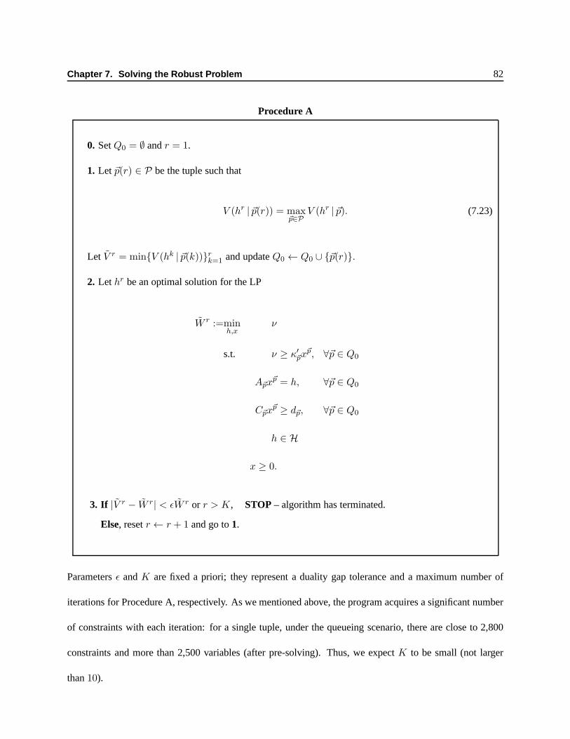
Chapter 7. Solving the Robust Problem 82
Procedure A
0. SetQ0 = ∅ andr = 1.
1. Let ~p(r) ∈ P be the tuple such that
V (hr | ~p(r)) = max~p∈P
V (hr | ~p). (7.23)
Let V r = min{V (hk | ~p(k))}rk=1 and updateQ0 ← Q0 ∪ {~p(r)}.
2. Let hr be an optimal solution for the LP
W r :=minh,x
ν
s.t. ν ≥ κ′~px~p, ∀~p ∈ Q0
A~px~p = h, ∀~p ∈ Q0
C~px~p ≥ d~p, ∀~p ∈ Q0
h ∈ H
x ≥ 0.
3. If |V r − W r| < εW r or r > K, STOP– algorithm has terminated.
Else, resetr← r + 1 and go to1.
Parametersε andK are fixed a priori; they represent a duality gap tolerance anda maximum number of
iterations for Procedure A, respectively. As we mentioned above, the program acquires a significant number
of constraints with each iteration: for a single tuple, under the queueing scenario, there are close to 2,800
constraints and more than 2,500 variables (after pre-solving). Thus, we expectK to be small (not larger
than10).

Chapter 7. Solving the Robust Problem 83
Once Procedure A terminates, we start Algorithm B, with the proviso that the master problem is initialized
as:
W r :=minz,h,x
z
s.t. z ≥ α′kh+ π′
kd~p(k), 1 ≤ k ≤ r − 1
z ≥ κ′~px~p, ∀~p ∈ Q0
A~px~p = h, ∀~p ∈ Q0
C~px~p ≥ d~p, ∀~p ∈ Q0
h ∈ H
x ≥ 0.
Algorithm B is then run as before. At each iterationr, Step 2 discovers a scenario~p(r), and Step 3 produces a
dual vector(πr, αr) which gives rise to the cutz ≥ α′rh+π′
rd~p(r) that is added to the master. The effect of the
enhancement provided by Procedure A is, typically, to drastically shortcut the number of iterations required
by Algorithm B; essentially, the algorithm has been hot-started with a very good initial representation of the
critical constraints needed to define problem (7.1).
7.3.1 Example 1 Revisited
To illustrate the performance of the enhanced Algorithm B, we present a number of statistics corresponding
to Example 1 for both the queueing and the threshold cost functions (Section6.1.1). For each iteration of
the algorithm we first point out if it is part of Procedure A (Enh_i) or if it is a regular iteration of Algorithm
B (Bend_i). We list its corresponding highest-cost tuple(p1, p2, d) and the lower and upper bounds on the
cost of the robust optimization problem. Finally we also addthe CPU time per iteration (in seconds) used to
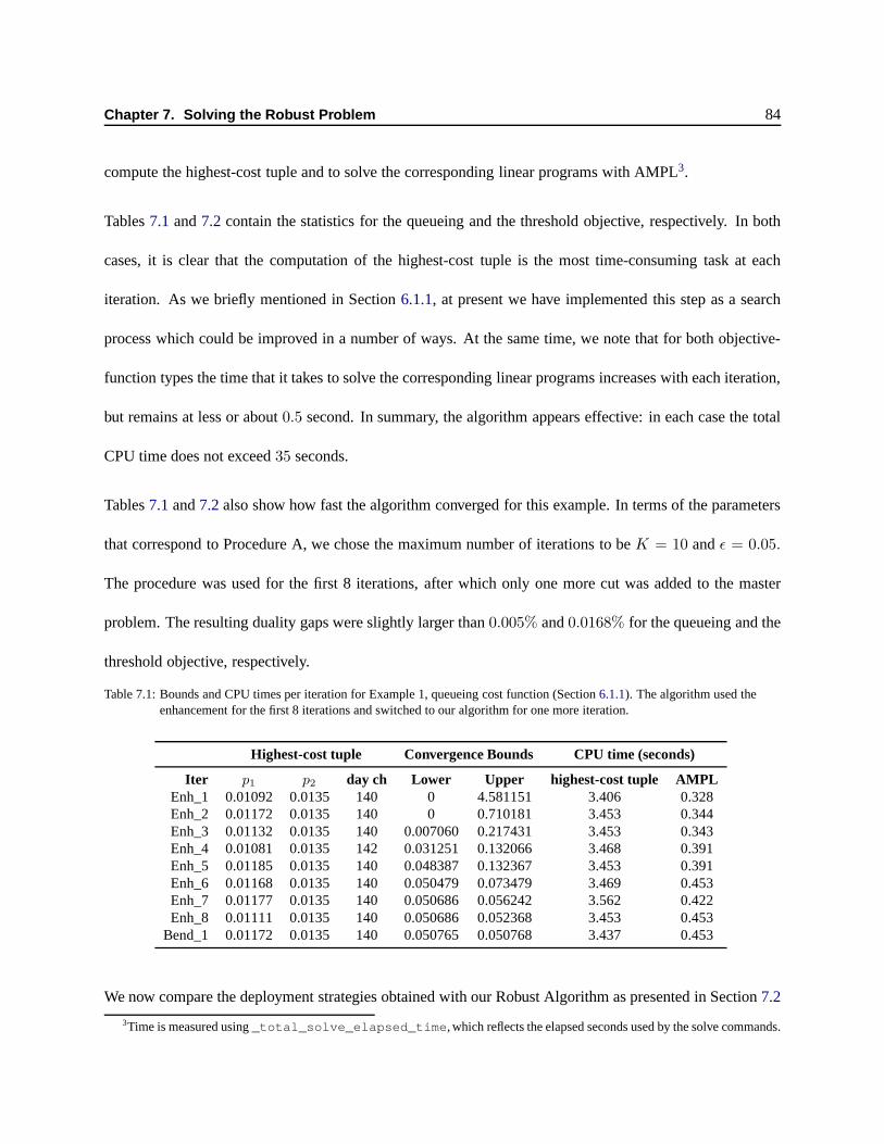
Chapter 7. Solving the Robust Problem 84
compute the highest-cost tuple and to solve the corresponding linear programs with AMPL3.
Tables7.1 and7.2 contain the statistics for the queueing and the threshold objective, respectively. In both
cases, it is clear that the computation of the highest-cost tuple is the most time-consuming task at each
iteration. As we briefly mentioned in Section6.1.1, at present we have implemented this step as a search
process which could be improved in a number of ways. At the same time, we note that for both objective-
function types the time that it takes to solve the corresponding linear programs increases with each iteration,
but remains at less or about0.5 second. In summary, the algorithm appears effective: in each case the total
CPU time does not exceed35 seconds.
Tables7.1and7.2also show how fast the algorithm converged for this example.In terms of the parameters
that correspond to Procedure A, we chose the maximum number of iterations to beK = 10 andε = 0.05.
The procedure was used for the first 8 iterations, after whichonly one more cut was added to the master
problem. The resulting duality gaps were slightly larger than0.005% and0.0168% for the queueing and the
threshold objective, respectively.
Table 7.1: Bounds and CPU times per iteration for Example 1, queueing cost function (Section6.1.1). The algorithm used theenhancement for the first 8 iterations and switched to our algorithm for one more iteration.
Highest-cost tuple Convergence Bounds CPU time (seconds)
Iter p1 p2 day ch Lower Upper highest-cost tuple AMPLEnh_1 0.01092 0.0135 140 0 4.581151 3.406 0.328Enh_2 0.01172 0.0135 140 0 0.710181 3.453 0.344Enh_3 0.01132 0.0135 140 0.007060 0.217431 3.453 0.343Enh_4 0.01081 0.0135 142 0.031251 0.132066 3.468 0.391Enh_5 0.01185 0.0135 140 0.048387 0.132367 3.453 0.391Enh_6 0.01168 0.0135 140 0.050479 0.073479 3.469 0.453Enh_7 0.01177 0.0135 140 0.050686 0.056242 3.562 0.422Enh_8 0.01111 0.0135 140 0.050686 0.052368 3.453 0.453
Bend_1 0.01172 0.0135 140 0.050765 0.050768 3.437 0.453
We now compare the deployment strategies obtained with our Robust Algorithm as presented in Section7.2
3Time is measured using_total_solve_elapsed_time, which reflects the elapsed seconds used by the solve commands.

Chapter 7. Solving the Robust Problem 85
Table 7.2: Bounds and CPU times per iteration for Example 1, threshold cost function (Section6.1.1). The algorithm used theenhancement for the first 8 iterations and switched to our algorithm for one more iteration.
Highest-cost tuple Convergence Bounds CPU time (seconds)
Iter p1 p2 day ch Lower Upper worst p AMPLEnh_1 0.01092 0.0135 140 32.23508 83.14448 2.891 0.343Enh_2 0.01168 0.0135 140 32.24410 37.34494 2.906 0.359Enh_3 0.01132 0.0135 140 32.25421 34.37022 2.875 0.406Enh_4 0.01081 0.0135 142 32.25740 33.12586 2.875 0.406Enh_5 0.01111 0.0135 140 32.25866 32.55180 2.891 0.437Enh_6 0.0109 0.0135 140 32.25912 32.33714 2.953 0.484Enh_7 0.01125 0.0135 140 32.25914 32.29835 2.922 0.485Enh_8 0.01118 0.0135 140 32.25915 32.27235 2.891 0.5
Bend_1 0.01091 0.0135 140 32.25915 32.26458 2.907 0.531
with the one from the improved version described in the present section.
In the case of the queueing objective, the Robust Algorithm has a worst-case cost of0.05214 with a duality
gap of close to5%; in turn, the enhanced algorithm has0.0507 and0.0052%, respectively. As depicted in
Figure7.1, the strategies follow the same pattern for the first 15 days,which trail the worst-case scenario
without intervention (as described in Section6.1.1). They later differ slightly albeit maintaining the same
general structure, which makes up for the difference in the duality gaps.
160
180
200
100
120
140
160
nt Strategy
40
60
80
100
Procuremen
0
20
40
25 27 29 31 33 35 37 39 41 43 45 47 49 51 53 55 57 59 61 63 65
P
Time from declaration of the epidemic
Robust Robust (Enhanced)
Figure 7.1: Resulting deployment strategies from our Robust Algorithm and its improved version.
On the other hand, the corresponding deployment strategiesfor the threshold cost function are quite different
(see Figure7.2a). At the same time, their worst-case costs are less than 1% apart: the strategy obtained
from the Robust Algorithm without improvements has a cost of32.45 with a duality gap of2.7% and

Chapter 7. Solving the Robust Problem 86
with enhancements,32.26 and0.017%, respectively. We hypothesize that the strategy obtained from the
Improved Algorithm is very influenced by the No-Action-Worst-Tuple, as evidenced by Figure7.2b, while
the Robust Strategy, obtained from an empty master problem,is void of such influence.
350
400
450
y
250
300
nt
Strategy
100
150
200
Deploymen
0
50
1 5 9 13 17 21 25 29 33 37 41 45 49 53 57 61 65 69 73 77
D
1 5 9 13 17 21 25 29 33 37 41 45 49 53 57 61 65 69 73 77
Time from declaration of the epidemic
Robust Robust (Improved)
(a) Robust Strategy compared to Improved Robust Strategy
200
250
y
150
nt
Strategy
50
100
Deploymen
0
50
1 5 9 13 17 21 25 29 33 37 41 45 49 53 57 61 65 69 73 77
D
1 5 9 13 17 21 25 29 33 37 41 45 49 53 57 61 65 69 73 77
Time from declaration of the epidemic
Naïve worst case Robust!(Improved)
(b) Improved Robust Strategy compared to Naïve-worst-caseStrategy
Figure 7.2: Comparison of deployment strategies obtained from our Robust Algorithm, our Improved Robust Algorithm, and theNaïve-worst-case strategy. Strategies correspond to Example 1, using the threshold cost function.
Chapter 8. Extensions 87
88Extensions
In this chapter we outline two extensions to our approach where the decision-maker can apply recourse when
conditions significantly deviate from predictions. From a broad optimization perspective such strategies
clearly make sense – why stick with a rigid strategy?. However, we stress that in view of the experiments
at the end of the last section, the likely benefit from a dynamic policy would be primarily realized during
a period immediately following the epidemic declaration and of relatively short duration. As as a result, a
decision maker would likely face severe logistical constraints if attempting to rapidly redeploy large numbers
of staff. Thus, a dynamic policy might only be able to performsmallchanges on a day-to-day basis. From
an operational perspective such small changes would of course make sense and would be applied; however
the recourse might only amount to a set of small adjustments to a pre-computed strategy.
In both cases that we consider we assume that a decision-maker can only approximately observe the behavior
of pt (the value ofp at time t). The Benders-decomposition solution methodology that wedescribed in

Chapter 8. Extensions 88
Chapter7 can be adapted to handle both models.
8.1 Robust optimization with recourse
Assume that uncertainty ofpt is modeled usingm intervals, ortranches, denotedI1, I2, . . . Im, for some
integerm > 0. In addition, two time periods are given,Jmin andJmax. A realization of the uncertain
valuespt plays out as follows:
(i) A period Jmin ≤ J ≤ Jmax is chosen, as well as a valuep(1) ∈ I1, a trancheH, and a value
p(2) ∈ H.
(ii) For eacht < J we havept = p(1) whereas for eacht ≥ J , pt = p(2).
In other words,pt is allowed to change values, once. The decision-maker operates as follows. First, a fixed
time period,S, in which the deployment strategy will berevisedis chosen in advance. Then
(a) At time t = 1, the decision-maker knows thatp1 ∈ I1, but does not know its precise value. The
decision-maker then produces an initial, or “first-stage” deployment plan indicating the amount of
staff to call-up at timet, for eacht < S. Further,m alternative “second-stage” deployment plans
(labeled1, 2, . . . ,m) are announced, each of which specifies the level of staff to deploy at each pe-
riod t ≥ S. Each second-stage plan is compatible with the first-stage plan in terms of deployment
constraints (such as total staff availability).
(b) At time t = S the decision-maker observes the tranche thatpS belongs to, but not the actual value of
pS . If trancheh is observed, then second-stage planh is rolled out on periodst ≥ S.

Chapter 8. Extensions 89
Example.Consider a case with three tranches:I2 = [.1, .15], I1 = [.15, .18], andI3 = [.18, .19]. Further,
Jmin = 18 andJmax = 60. A realization of the data is the following:J = 20, p(1) = .155, H = I3
andp(2) = .19. Thus, fort < 20 we havept = .155 while for t ≥ 20, pt = .19. SupposeS = 30. The
decision-maker knows that.15 ≤ p1 ≤ .18; at timeS = 30 the decision-maker observes the trancheI3 and
thus knows that fort ≥ 30, .18 ≤ pt ≤ .19, leading to an appropriate set of deployments for future periods.
The model we just described is inherently adversarial: it assumes that, subject to the stated rules, data will
take on worst-case attributes. This feature can, of course,lead to overly conservative plans. However, the
proper statement to make is that the plans will be conservative only if the data (the tranches, in particular)
allow it to be so. A different drawback in this model is that anadversary could simply “wait” to changep
until just after the review periodS. As the experiments in Section6.1.3indicate, ifS is not too small the
impact of such a late change inp is much decreased. IfS is chosen too large, then the adversary can change
p much earlier, and then the impact will be felt before the review can take place. Thus, care must be chosen
in selectingS. A review strategy that proceeds dynamically is given next.
8.2 Stochastic optimization
In contrast to the above, we also outline a model where the contagion probabilitiespt behave stochastically.
Assume:
(i) p1 takes a random value drawn from a uniform distribution over aknown intervalZ.
(ii) For any t, pt+1 = pt + εt, whereεt is normally distributed, with zero mean and small standard
deviation (small compared to the width ofZ).

Chapter 8. Extensions 90
Thus, pt executes a random walk, starting fromZ. Let p indicate the center (mean value) ofZ. The
decision-maker’s actions, in this model, are as follows.
(a) At time t = 1, the decision-maker produces a policy consisting of a triple (h, α, R) whereα ≥ 0,
andh is an initial staff surge deployment plan indicating for each t the quantityht, the amount of staff
to call-up at timet. Finally, the decision-maker also places an additional quantity R ≥ 0 of surge-staff
on reserve (i.e., not yet part of the deployment plan). For notational purposes, writeht = ht, for
eacht.
(b) The decision-maker can revise the plan at any of several checkpointst1 < t2 < . . . < tr.
(c) Consider checkpointti (1 ≤ i ≤ m). Let
Θ(ti, p) = the total number individuals infected by timeti, in the SEIR model wherept = p,
for 1 ≤ ti
Γ(ti) = theactual total number of individuals who are infected by timet.
Thus,Θ(ti, p) is an estimate of the random variableΓ(ti). We assume that the decision-maker ob-
serves, as an estimate forΓ(ti), a quantity
ν(i) = Γ(ti) + δ(ti), (8.1)
whereδ(ti) is normally distributed with zero mean and known variance. Then, the deployment plan
is revised as follows. Write
∆ =ν(i) − Θ(ti, p)
ti.

Chapter 8. Extensions 91
Then, the decision-maker resets
ht ← ht + α∆, for eachti ≤ t < ti+1, and (8.2)
R ← R − (ti+1 − ti)α∆. (8.3)
Comment.The proposed scheme constitutes an example of affine control. The decision-maker computes
an initial estimate of the deployment plan (the initialht) which are corrected on the basis of real-time
observations, using the parameterα to modulate the corrections. The quantity∆ indicates the (per-period)
deviation between the observed behavior of the epidemic (including “noise”, given byδ) and the predicted
behavior as given byΘ(th, p).
When∆ > 0, the behavior of the epidemic is worse than initially estimated and Rule (8.2) will increase
the near-future surge staff deployment. This increase is drawn from the surge staff held in reserve, as per
equation (8.3). When∆ < 0, (8.3) moves staff back into the reserve ranks.
Note that in order for Rule (8.3) to be feasibly applied, the resultingR must benonnegative. For this to
be the case when∆ > 0 we should haveα small enough, and, especially, that the initial estimate for R be
“high enough.” These are constraints to be maintained in oursolution algorithms.
In order to consider algorithmic implications of this model, consider a fixedsample pathspecifying a value
for eachpt and for eachδ(ti) (see equation (8.1)). Denote byT the length of the planning horizon. Recall
that in the stochastic model the decision-maker announces,at t = 1, a triple(h, α,R). We have:
Lemma 8.2.1 Under the given sample path the cost incurred by the policy(h, α,R) (as per rules (b)-(c) )
is given by a linear program whose right-hand side is an affinefunction of theht andα.
Chapter 8. Extensions 92
As a consequence, we expect that several well-known methodologies for stochastic optimization, such as
sample average approximation[69], [70] and stochastic gradient schemes[68], [46], will be well-suited for
our problem.

Discussion 93
99Discussion
The potential impact of a severe influenza epidemic on essential services is a matter of critical importance
from a public health perspective. There are current concerns that an influenza virus might mutate into
a highly contagious strain for which humans have little or noimmunity, resulting in a rapid widespread
of the disease. In the event of such an epidemic or pandemic, organizations that provide critical social
infrastructure, such as health care clinics, police departments, public utilities, food markets, and supply
chains are likely to face severe workforce shortage that would jeopardize their continuity of operations. In
particular, at the most critical stage of the epidemic, health care clinics would be required to provide care
for an extraordinary number of patients, and thus could ill-afford staff shortfalls.
Pandemic influenza preparedness would require an extensiveset of challenging steps. It requires the in-
volvement and commitment of many segments of the academic, industrial and governmental communities.
The planning process requires joint efforts to improve, among other things, the vaccine and anti-viral de-

Discussion 94
velopment and distribution, the surveillance systems, andthe design of pragmatic and effective regional
plans. These plans must include, among other important activities, methods to expand surge capacity and to
maintain essential services, including the deployment of ‘surge’ staff to compensate for potential abnormal
absenteeism rates. To address these issues, the CDC and the HHS Department together with State authorities
have published suggested courses of action.
The intelligent design of such contingency plans would necessarily model the spread of the epidemic. In
the case of a new strain of the influenza virus, such modeling entails incorporating significant uncertainty:
as far as we know, there are no clear ways of accurately predicting the transmissibility of a new virus strain.
Moreover, it has been suggested that the effective contagion rate may change under different environmental
conditions, such as weather, which are likewise unpredictable. Additionally, social patterns may change
during the epidemic, for example due to the implementation of public health measures such as quarantine or
social distancing.
Pre-event planning is critical: once pandemic flu strikes a community, it could be over in few months,
barely enough time to put together all the elements of emergency management that we have extensively
described. We believe Robust Optimization is the best tool to tackle the problem from this perspective,
particularly because of the sheer unpredictability of the epidemics’ intensity and length. Although it could
be deemed too conservative (in a way, it is optimizing against the worst-case scenario), this methodology
effectively immunizes the solutions against a pre-specified uncertainty set. This could prove invaluable from
a social cost perspective. Moreover, a decision-maker interested in using our tool could vary the degree of
risk aversion by varying the structure of the uncertainty set: the size of the intervals that conform it is
proportional to the degree of risk aversion. Several scenarios could be considered until a balanced tradeoff
is reached.

Discussion 95
In this thesis we build a tool that helps to study how to designrobust pre-planned surge staff deployment
strategies that would aide an organization to cope with workforce shortfalls while optimally hedging against
uncertainty. As far as we know, this is the first time that thismethodology is used in this research area. As
discussed in previous chapters, earlier work primarily focuses on conducting simple sensitivity analysis as
a way to measure robustness. These works implicitly assume probability distributions on the parameters
when these may not be readily available or are easily justifiable. Our models do not need to make such
assumptions.
Taking advantage of a version of the generalized Benders’ Decomposition, we propose fast and accurate
algorithms that prove sufficiently flexible to incorporate intricate uncertainty sets that reflect the change-
ability of the environment. We bring insights on the structure of optimal robust strategies and on practical
rules-of-thumb that can be deployed during the epidemic.
To benchmark the effectiveness of the obtained robust policies, we compared them to the policies that opti-
mally solve the problem for the scenario with highest cost given that no action is taken (the Naïve-worst-case
Policy). Our proposed solutions could also be compared to policies obtained from an equivalent Stochastic
Optimization problem, which minimize the average cost overall possible scenarios within the uncertainty
set. While this is a useful exercise, we use the Naïve-worst-case Policy as a first benchmark because pre-
paredness plans often suggest decision makers to augment their surge capacity based on a scenario similar
to the Spanish Flu. This is considered to be theworst influenza pandemic known by human kind (in terms of
mortality and social impact). Our results show that following a strategy that just considers the highest-cost
scenario may allocate resources inappropriately for milder cases, which are also likely to occur. This would
translate in big savings for a decision maker: surge capacity would be effectively used inanyscenario within
the preestablished uncertainty set avoiding wastage. We expect the comparison of our Robust Strategy to
Discussion 96
one obtained from a Stochastic Optimization framework to yield similar results and leave it as an extension
of this thesis.
Our strategies also behave well in out-of-sample tests in which the probability of contagion was allowed to
change to larger values outside the uncertainty set, and at least 10 days after the surge staff started to be de-
ployed. A notable fact was that whenp changes relatively late with respect to the strategy’s deployment, the
epidemic has largely run its course and the change doesn’t have any meaningful impact. When the change
occurs much earlier, social distancing prevents the epidemic from unfolding, highlighting the importance
of these kind of interventions. Further out-of-sample tests suggested that it may be desirable to include a
lateness factor in the uncertainty set.
A number of refinements and extensions of this thesis are possible. First, one could include a more spe-
cific compartmental model for influenza: adding more population subgroups to the model should be able to
capture population dynamics better; similarly, incorporating more compartments would describe the disease
more accurately (such as an asymptomatic compartment, as presented in Chapter 12 of[15]). These en-
hancements would have to handled with care, for they would require corresponding parameter values. Data
paucity could represent a disadvantage more than a benefit.
A second extension would incorporate the potential impact that a staff contingency plan could have on the
course of the epidemic (so far assumed to be negligible). This could be the case, for instance, at vaccination
centers; their adequate staffing could be crucial to reach critical vaccination fractions in a timely matter.
We did not venture into this endeavor because any such model would heavily rely on the ability of the
surge staff to change the epidemic dynamics. In the case of the vaccination centers, an effective vaccine
would have to be readily available. For a new flu virus mutation it is unclear whether this is possible,

Discussion 97
especially considering that influenza vaccines take at least 6 months to manufacture. Thus, this extension
would be useful should the model be used for seasonal influenza or for epidemics for which effective means
of fighting it are accessible and their deployment depends onthe effective implementation of a pre-specified
contingency plan.
Another extension includes the use of cross-staffing, either within a hospital or a network of clinics and
institutions. In this study we are considering the entire workforce of a particular organization as a whole;
however, as part of the contingency plans proposed by the CDC, organizations are encouraged to identify
critical staff positions and cross-train personnel accordingly. The model could also be further refined by
modeling more than one employee group depending on levels ofexposure to the disease or social contact
patterns. This would, of course, vary from organization to organization and should be tailored judiciously.
Our methods could be easily used to manage any quantifiable scarce resource during an epidemic. Moreover,
it is very likely that a decision-maker will face parallel resource problems during such an event - for example,
a hospital would need to plan for bedding and other supplies on top of surge staffing. Any multiple-objective
cost function could be incorporated provided it has a convexpiecewise-linear shape. One such example
involves antiviral inventory management. In the case of hospitals and clinics, rates of transmission for health
care workers may be minimized during a severe pandemic by means of protective equipment or the use of
antiviral medication. Given that stockpiles are limited, ahospital could be interested in managing the doses
during the outbreak. Appropriate extensions to theSEIR model could be carefully made to accommodate
the reduction on disease transmissibility, while keeping track of the antiviral stockpile. Additionally, our
model currently assumes that surge staff is not exposed to the epidemic until they are called into service.
This relatively strong assumption could be remedied by incorporating properSEIR constraints to the linear
program defined byV (h|p) (see Chapter5); we also leave this for future projects.

Discussion 98
Finally, from an operational perspective, organizations may be able to react to evolutions of the epidemic
that significantly differ from initial estimations. While the space for action could be limited (from what
we learned from our out-of-sample tests), the topic is clearly of great interest. How to incorporate optimal
recourse decisions is a topic we briefly discussed in Chapter8 and plan to address in future work.

Bibliography 99
Bibliography
[1] Operations research and public health.American Journal of Public Health and the Nations Health,42(10):1306–1307, October 1952.
[2] The world’s deadliest bioterrorist.The Economist, April 28th 2012.
[3] Dionne M. Aleman. Predicting the spread of pandemic disease. OR/MS Today, 39:24–28, February2012.
[4] L.J.S. Allen and A.M. Burgin. Comparison of deterministic and stochastic sis and sir models in discretetime. Mathematical biosciences, 163(1):1–33, 2000.
[5] LJS Allen, MA Jones, and CF Martin. A discrete-time modelwith vaccination for a measles epidemic.Mathematical biosciences, 105(1):111–131, 1991.
[6] L.J.S. Allen and P. van den Driessche. The basic reproduction number in some discrete-time epidemicmodels.Journal of Difference Equations and Applications, 14(10):1127–1147, 2008.
[7] R.M. Anderson and R.M. May.Infectious diseases of humans: dynamics and control, volume 26.Wiley Online Library, 1992.
[8] Command center operations. http://apogeeengineering.net/index.cfm/ID/54/Command-Center-Operations/, 2012.
[9] J. Arino, F. Brauer, P. Van Den Driessche, J. Watmough, and J. Wu. Simple models for containment ofa pandemic.Journal of the Royal Society Interface, 3(8):453, 2006.
[10] J.G. Bartlett. Planning for avian influenza.Annals of internal medicine, 145(2):141–144, 2006.

Bibliography 100
[11] J.G. Bartlett and L. Borio. The current status of planning for pandemic influenza and implications forhealth care planning in the united states.Clinical Infectious Diseases, 46(6):919, 2008.
[12] A. Ben-Tal and A. Nemirovski. Robust optimization–methodology and applications.MathematicalProgramming, 92(3):453–480, 2002.
[13] J.F. Benders. Partitioning procedures for solving mixed-variables programming problems.NumerischeMathematik, 4(1):238–252, 1962.
[14] M.C.J. Bootsma and N.M. Ferguson. The effect of public health measures on the 1918 influenzapandemic in US cities.Proceedings of the National Academy of Sciences, 104(18):7588, 2007.
[15] F. Brauer, P. Van den Driessche, J. Wu, and L.J.S. Allen.Mathematical epidemiology. Number 1945.Springer Verlag, 2008.
[16] C.B. Bridges, M.J. Kuehnert, and C.B. Hall. Transmission of influenza: implications for control inhealth care settings.Clinical Infectious Diseases, pages 1094–1101, 2003.
[17] Flu surge 2.0. http://www.cdc.gov/flu/tools/flusurge/, August 2011.
[18] Seasonal influenza (flu). Retrieved October, 2011. http://www.cdc.gov/flu/, 2011.
[19] G. Chowell, S. Echevarría-Zuno, C. Viboud, L. Simonsen, J. Tamerius, M.A. Miller, and V.H. Borja-Aburto. Characterizing the epidemiology of the 2009 influenza a/h1n1 pandemic in mexico.PLoSMed, 8[5]:e1000436, 2011. Available at doi:10.1371/journal.pmed.1000436.
[20] G. Chowell, H. Nishiura, and L. Bettencourt. Comparative estimation of the reproduction number forpandemic influenza from daily case notification data.Journal of the Royal Society Interface, 4(12):155,2007.
[21] MD Cinti, Sandro, MD Chenoweth, Carol, and MD Monto, Arnold S. Preparing for pandemicinfluenza: Should hospitals stockpile oseltamivir?Infection Control and Hospital Epidemiology,26(11):pp. 852–854, 2005.
[22] Derek DeLia.Hospital Capacity, Patient Flow, and Emergency DepartmentUse in New Jersey. RutgersCenter for State Health Policy, 2007.
[23] O. Dieckmann and JP Heesterbeek.Mathematical epidemiology of infectious diseases. Wiley, NewYork, 2000.

Bibliography 101
[24] John N. Tsitsiklis Dimitris Bertsimas.Introduction to Linear Optimization. Athena Scientific Belmont,MA, 1997.
[25] L. ElGhaoui and H. Lebret. Robust solutions to least-squares problems with uncertain data.SIAM J.Matrix Anal. App., 18(4):1035–1064, 1997.
[26] Centers for Disease Control and Prevention. Flu view. aweekly influneza surveillance report preparedby the influenza division. Reviewed on October 2011. http://www.cdc.gov/flu/weekly/.
[27] E. Yoko Furuya, May 2011. Assistant Professor of Clinical Medicine, Division of Infectious Diseases,Columbia University Medical Center. Personal communication.
[28] M. Gardam, D. Liang, S.M. Moghadas, J. Wu, Q. Zeng, and H.Zhu. The impact of prophylaxis ofhealthcare workers on influenza pandemic burden.Journal of the Royal Society Interface, 4(15):727,2007.
[29] Pandemic influenza preparedness and response standardoperating guide. Available athttp://health.state.ga.us/pandemicflu, June 2006.
[30] R.R.M. Gershon, K.A. Qureshi, P.W. Stone, M. Pogorzelska, A. Silver, M.R. Damsky, C. Burdette,K.M. Gebbie, and V.H. Raveis. Home health care challenges and avian influenza.Home Health CareManagement & Practice, 20(1):58, 2007.
[31] C.D. Gomersall, S. Loo, G.M. Joynt, and B.L. Taylor. Pandemic preparedness.Current opinion incritical care, 13(6):742, 2007.
[32] M.L. Grayson, S. Melvani, J. Druce, I.G. Barr, S.A. Ballard, P.D.R. Johnson, T. Mastorakos, andC. Birch. Efficacy of soap and water and alcohol-based hand-rub preparations against live h1n1 in-fluenza virus on the hands of human volunteers.Clinical Infectious Diseases, 48(3):285, 2009.
[33] L.V. Green and P.J. Kolesar. Improving emergency responsiveness with management science.Man-agement Science, pages 1001–1014, 2004.
[34] M.S. Green, T. Swartz, E. Mayshar, B. Lev, A. Leventhal,P.E. Slater, and J. Shemer. When is anepidemic an epidemic?Israel Medical Association Journal, 4(1):3–6, 2002.
[35] M. Grötschel, L. Lovász, and A. Schrijver. The ellipsoid method and its consequences in combinatorialoptimization.Combinatorica, 1(2):169–197, 1981.
Bibliography 102
[36] M.E. Halloran, N.M. Ferguson, S. Eubank, I.M. Longini,D.A.T. Cummings, B. Lewis, S. Xu,C. Fraser, A. Vullikanti, T.C. Germann, et al. Modeling targeted layered containment of an influenzapandemic in the United States.Proceedings of the National Academy of Sciences, 105(12):4639, 2008.
[37] J.L. Hick, M.D. Christian, and C.L. Sprung. Chapter 2. surge capacity and infrastructure considerationsfor mass critical care.Intensive care medicine, 36:11–20, 2010.
[38] A.N. Hill, I.M. Longini, et al. The critical vaccination fraction for heterogeneous epidemic models.Mathematical biosciences, 181(1):85–106, 2003.
[39] J. Hoffbuhr. Utilities prepare for potential pandemic. American Water Works Association Journal,98(6):48–60, 2006.
[40] Implementation plan for the national strategy for pandemic influenza. Last accessed June 2012. Avail-able at www.flu.gov/planning-preparedness/federal/pandemic-influenza.pdf, May 2006.
[41] Edward Kaplan. Operations research and public health.University Lecture.
[42] M.J. Keeling and P. Rohani.Modeling infectious diseases in humans and animals. Princeton UniversityPress, 2008.
[43] W.O. Kermack and A.G. McKendrick. Contributions to themathematical theory of epidemics. ii. theproblem of endemicity.Proceedings of the Royal society of London. Series A, 138(834):55–83, 1932.
[44] WO Kermack and AG McKendrick. Contributions to the mathematical theory of epidemics. iii. fur-ther studies of the problem of endemicity.Proceedings of the Royal Society of London. Series A,141(843):94–122, 1933.
[45] WO Kermack and AG McKendrick. Contributions to the mathematical theory of epidemicsUi. Bulletinof mathematical biology, 53(1):33–55, 1991.
[46] H.J. Kushner and D.S. Clark.Stochastic approximation methods for constrained and unconstrainedsystems. Springer, 1978.
[47] R.C. Larson. Simple models of influenza progression within a heterogeneous population.Operationsresearch, 55(3):399–412, 2007.
[48] H.L. Lee, V. Padmanabhan, and S. Whang. The bullwhip effect in supply chains1.Sloan managementreview, 38(3):93–102, 1997.

Bibliography 103
[49] V.J. Lee and M.I. Chen. Effectiveness of neuraminidaseinhibitors for preventing staff absenteeismduring pandemic influenza.Emerging Infectious Diseases, 13(3):449, 2007.
[50] I.M. Longini Jr, M.E. Halloran, A. Nizam, and Y. Yang. Containing pandemic influenza with antiviralagents.American Journal of Epidemiology, 159(7):623, 2004.
[51] I.M. Longini Jr, A. Nizam, S. Xu, K. Ungchusak, W. Hanshaoworakul, D.A.T. Cummings, and M.E.Halloran. Containing pandemic influenza at the source.Science, 309(5737):1083, 2005.
[52] A.C. Lowen, S. Mubareka, J. Steel, and P. Palese. Influenza virus transmission is dependent on relativehumidity and temperature.PLoS pathogens, 3(10):e151, 2007.
[53] C.E. Mills, J.M. Robins, and M. Lipsitch. Transmissibility of 1918 pandemic influenza.Nature,432(7019):904–906, 2004.
[54] N.A.M. Molinari, I.R. Ortega-Sanchez, M.L. Messonnier, W.W. Thompson, P.M. Wortley, E. Wein-traub, and C.B. Bridges. The annual impact of seasonal influenza in the us: measuring disease burdenand costs.Vaccine, 25(27):5086–5096, 2007.
[55] S.S. Morse. Building academic-practice partnerships: the Center for Public Health Preparedness atthe Columbia University Mailman School of Public Health, before and after 9/11.Journal of PublicHealth Management and Practice, 9(5):427, 2003.
[56] Stephen Morse, February 2011. Professor of Clinical Epidemiology, Founding Director & Senior Res.Scientist, Center for Public Health Preparedness. Personal communication.
[57] Influenza pandemic plan guide for healthcare facilities. Available athttp://www.nj.gov/health/flu/plan.shtml, August 2005.
[58] Pandemic preparedness planning template for federally qualified health centers. July 2007.
[59] Facts and statistics 2010. Retrieved October, 2011. http://nyp.org/about/facts-statistics.html, 2010.
[60] A.T. Newall, J.G. Wood, N. Oudin, and C.R. MacIntyre. Cost-effectiveness of Pharmaceutical-basedPandemic Influenza Mitigation Strategies.Strategies, 2:3.
[61] M. Nuno, G. Chowell, and AB Gumel. Assessing the role of basic control measures, antivirals andvaccine in curtailing pandemic influenza: scenarios for theus, uk and the netherlands.Journal of theRoyal Society Interface, 4(14):505–521, 2007.

Bibliography 104
[62] Emergency management. Retrieved July, 2011. http://www.nyc.gov/html/doh/html/em/emergency-homepage.shtml, 2011.
[63] What employers can do to protect workers from pandemic influenza. Retrieved May, 2011.http://www.osha.gov/Publications/employers-protect-workers-flu-factsheet.html, 2009.
[64] National Institute of Allergy and Infectious Diseases. Flu (influenza). Retrieved May 1, 2012.http://www.niaid.nih.gov/topics/flu/understandingflu/pages/definitionsoverview.aspx, August 2011.
[65] Department of Transportation. Pandemic flu planning, March 2009. http://www.dot.gov/pandemicflu/.
[66] M.T. Osterholm. Preparing for the next pandemic.New England Journal of Medicine, 352(18):1839,2005.
[67] Raúl Rabadán, November 2010. Assistant Professor of Biomedical Informatics, Columbia UniversityCollege of Physicians and Surgeons. Personal communication.
[68] H. Robbins and S. Monro. On a stochastic approximation method.Annals of Mathematical Statistics,22:400–407, 1951.
[69] A. Shapiro and H. Homem de Mello. On rate of convergence of monte carlo approximations of stochas-tic programs.SIAM J. on Optimization, 11:70–86, 2001.
[70] D. Shmoys and C. Swamy. Sampling-based approximation algorithms for multi-stage stochastic opti-mization.Proc. FOCS 2005, pages 357–366, 2005.
[71] J. Taubenberger and D. Morens. 1918 Influenza: the mother of all pandemics.Rev Biomed, 17:69–79,2006.
[72] B.L. Taylor, H.E. Montgomery, A. Rhodes, and C.L. Sprung. Chapter 6. protection of patients andstaff during a pandemic.Intensive care medicine, 36:45–54, 2010.
[73] Swine flu (h1n1 virus). Retrieved May, 2011. http://nyti.ms/SiDWD, January 2010.
[74] The evolution of bird flu, and the race to keep up. Retrieved June, 2012. http://nyti.ms/N2g7mi, June2012.
[75] S. Towers and Z. Feng. Pandemic h1n1 influenza: Predicting the course of vaccination programme inthe united states.Eurosurveillance, 14, 2009.

Bibliography 105
[76] Lauren Trainor, Joseph; Barsky. Reporting for duty? a synthesis of research on role conflict, strain,and abandonment among emergency responders during disasters and catastrophes. Technical report,Disaster Research Center, 2011. Available at http://dspace.udel.edu:8080/dspace/handle/19716/9885.
[77] Business planning. Last accessed July 2011. http://www.pandemicflu.gov.
[78] Pandemic influenza plan, supplement 3, healthcare planning.http://www.hhs.gov/pandemicflu/plan/sup3.html.
[79] J. Wallinga, P. Teunis, and M. Kretzschmar. Using data on social contacts to estimate age-specifictransmission parameters for respiratory-spread infectious agents.American Journal of Epidemiology,164(10):936, 2006.
[80] J. Wallinga, M. Van Boven, and M. Lipsitch. Optimizing infectious disease interventions during anemerging epidemic.Proceedings of the National Academy of Sciences, 107(2):923, 2010.
[81] What is public health? Retrieved June, 2012. http://www.whatispublichealth.org/.
[82] What is a pandemic? Reviewed on May, 2012. http://www.who.int/csr/disease/swineflu/en/.
[83] J.T. Wu, S. Riley, C. Fraser, and G.M. Leung. Reducing the impact of the next influenza pandemicusing household-based public health interventions.PLoS Med, 3(9):e361, 2006.