CLASS NOTES

Models, Algorithms and Data: Introduction to computing

2018

Petros Koumoutsakos, Jens Honore Walther

(Last update: April 16, 2018)

IMPORTANT DISCLAIMERS

1. REFERENCES: Much of the material (ideas, definitions, concepts, examples, etc) in

these notes is taken (in some cases verbatim) for teaching purposes, from several references,

and in particular the references listed below. A large part of the lecture notes is adapted from

The Nature of Mathematical Modeling by Neil Gershenfeld (Cambridge University Press, 1st ed.,

1998). Therefore, these notes are only informally distributed and intended ONLY as study aid

for the final exam of ETHZ students that were registered for the course Models, Algorithms and

Data (MAD): Introduction to computing 2018.

2. CONTENT: The present Notes are a first LaTex draft for the Lectures of Models, Algo-

rithms and Data (MAD): Introduction to computing. The notes have been checked but there is

no guarantee that they are free of mistakes. Please use with care. Again, these notes are only

intended for use by the ETHZ students that were registered for the course Models, Algorithms

and Data (MAD): Introduction to computing 2018 and ONLY a study aid for their final exam.

Chapter 5

Solving Non-Linear Equations

5.1 Key Points

After this class, you should understand the following points regarding the solution of non-linear

equations:

• What are the key algorithms for non-linear equation solving

• When to use derivatives or their approximation in Newton’s methods

• What is the Jacobian for Newton’s method and what is its role

• Why do we approximate the Jacobian in Newton’s methods

2 Chapter 5. Solving Non-Linear Equations

5.2 Introduction

So far we have looked at linear systems of equations. For N linear equations with N unknowns,

we wrote as A~x = ~b, where A is an invertible N × N matrix and ~x and ~b are vectors of length

N . For function fitting, we determined A and ~b from the data and computed the N unknown

parameters in ~x by solving the system A~x = ~b. The equivalent would be to solve the linear set

of equations ~F (~x) = A~x−~b = 0.

The task becomes harder if we try to find the solution for a general system of N non-linear

equations fi(~x) (i = 1, . . . , N), where ~x = (x1, . . . , xN ) is a vector of N unknowns. We wish to

find ~x∗, such that fi( ~x∗) = 0 (i = 1, . . . , N). We commonly write this system as ~F ( ~x∗) = ~0.

For a single non-linear equation f(x) the problem reduces to finding the x∗ such that

f(x∗) = 0. (5.2.1)

This means that x∗ is a root (zero) or the function f(x). The problem of solving a non-linear

equation is thus a root-finding problem. Looking at the graph of f(x) below the goal is to find

points, where the curve crosses the horizontal axis.

f(x)

x

x* x*

Example with one unknown: Population growth (adapted from book Numerical Analysis by

R.L. Burden and J.D. Faires)

Let N(t) be the number of people at time t. Let λ be the birth rate. Then the equation describing

the population growth has the form:

dN(t)

dt= λN(t). (5.2.2)

Assume that we also have an immigration at a constant rate u. Then the population growth

equation will include an additional term:

dN(t)

dt= λN(t) + u. (5.2.3)

5.3. Preliminaries 3

The solution of the Eq. (5.2.3) is given by the following formula:

N(t) = N0eλt +

u

λ(eλt − 1), (5.2.4)

where N0 is a constant indicating the initial population size.

Numerical example. Suppose we have initially 1,000,000 people. Assume that 15,000 people

immigrate every year and that 1,080,000 people are present at the end of the year. What is the

birth rate of this population?

To find the birth rate we need to solve the following equation for λ (remember that t = 1 [year]):

1, 080, 000 = 1, 000, 000eλ +15, 000

λ(eλ − 1). (5.2.5)

Example for a system:

The amount of pressure required to sink a large heavy object in a soft homogeneous soil that

lies above a hard base soil can be predicted by the amount of pressure required to sink smaller

objects.

Let p denote the amount of pressure required to sink a circular plate of radius r at a distance

d in the soft soil, where the hard soil lies at a distance D > d below the surface. p can be

approximated by an equation of the form:

p = k1ek2r + k3r, (5.2.6)

where k1, k2, k3 depend on d and the consistency of the soil but not on r.

Now the task is to find k1, k2, k3. To do that we need to have 3 equations which we can obtain by

taking plates of different radii r1, r2, r3 and sinking them. After doing so we will get the following

system of equations:

p1 = k1ek2r1 + k3r1,

p2 = k1ek2r2 + k3r2, (5.2.7)

p3 = k1ek2r3 + k3r3.

In both examples, we are dealing with non-linear equations and the question is how one can solve

such equations.

5.3 Preliminaries

Existence and Uniqueness

The first question we need to answer is whether the root (i.e., the solution) to our problem exists.

Recall that for linear problems finding the solution of A~x = ~b required that A−1 6= 0 or that A is

4 Chapter 5. Solving Non-Linear Equations

non-singular. To determine this criterion for a non-linear equation, we look at the Intermediate

Value Theorem.

Intermediate Value Theorem:

If a function f(x) is continuous on interval [a, b] and K any number between f(a) and f(b), then

there exists a number x∗ ∈ (a, b) for which f(x∗) = K.

Consequence:

If a function f(x) is continuous on interval [a, b] with f(a) and f(b) of opposite sign, i.e.,

f(a)f(b) < 0 then according to Intermediate Value Theorem there is a x∗ ∈ (a, b) with f(x∗) = 0.

Note: There is no simple analog of this theorem for the multi-dimensional case.

Sensitivity and Conditioning

If a solution to the problem exists, the second question to ask is whether we will find this

solution with some algorithm. Consider an approximate solution x to f(x) = 0, where x∗ is the

true solution.

‖f(x)‖ ≈ 0 → ‖x− x∗‖ ≈ 0, (5.3.1)

A small residual ‖f(x)‖ implies an accurate solution (i.e., ‖x− x∗‖ ≈ 0) only if the problem is

well-conditioned. Note that the true solution x∗ is not known apriori, thus we can only evaluate

‖f(x)‖.The problem is well-conditioned if a small change in the ”input” causes a small change in the

”output”. The problem is ill-conditioned if a small change in the ”input” causes a large change

in the ”output”. How well or ill-conditioned is a problem is measured by the condition number:

κ =|δy||δx| , (5.3.2)

where δx is the change in the input, δy is the change in the output and y = f(x). δy = f(x +

δx)−f(x) and f(x+δx) can be expanded using Taylor series as f(x+δx)−f(x) ≈ f(x)+f ′(x)δx,

where we have neglected higher order terms. Therefore, δy ≈ f ′(x)δx and κ = |f ′(x)|. This is a

condition number for a function evaluation, i.e, when given x we evaluate y.

The root-finding problem is a reverse problem to function evaluation. For a root x∗ of a function

f(x) we can write x∗ = f−1(y) = g(y), where f−1 is an inverse function and thus the conditioning

of root finding problem is given by

κ = |g′(y)| = | ∂∂y

[f−1(y)]| = 1

|f ′ (x∗)| . (5.3.3)

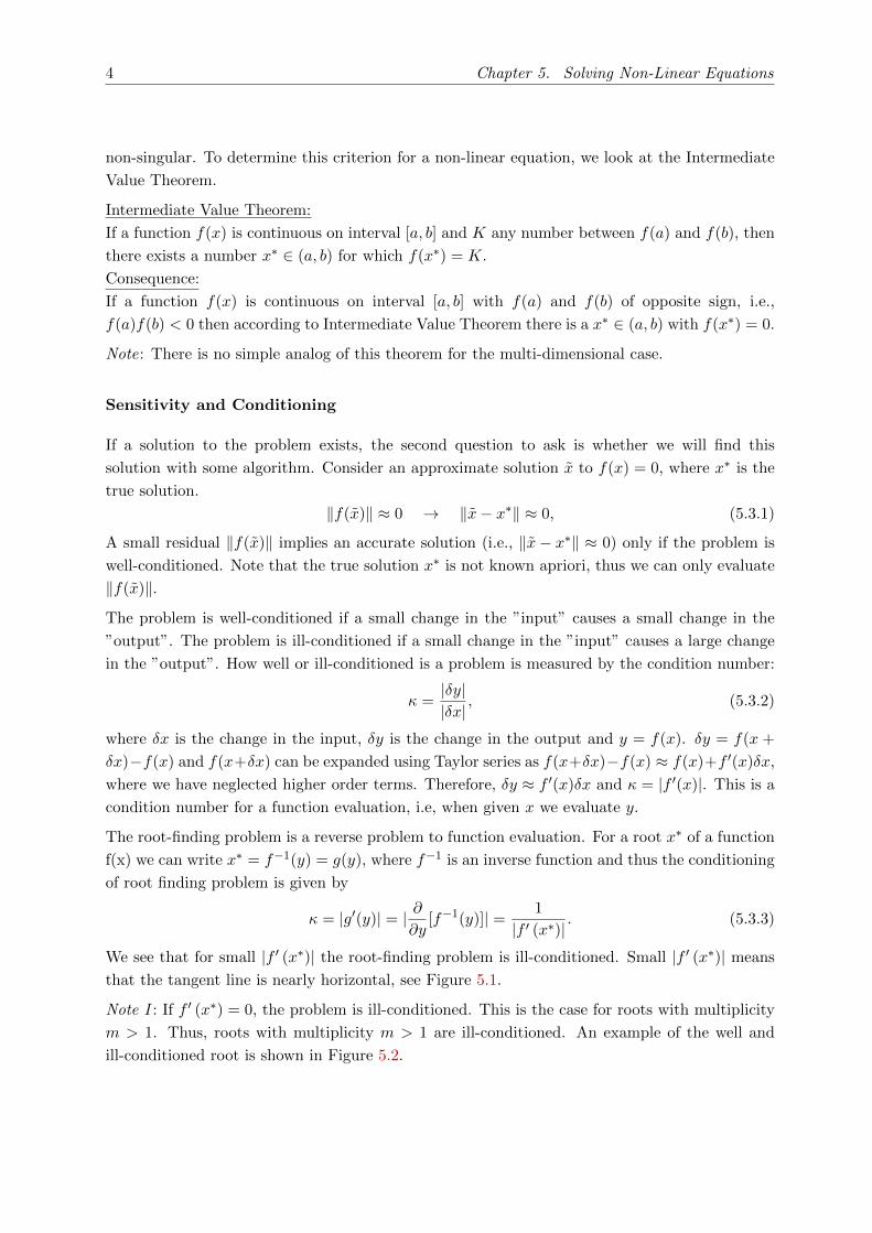
We see that for small |f ′ (x∗)| the root-finding problem is ill-conditioned. Small |f ′ (x∗)| means

that the tangent line is nearly horizontal, see Figure 5.1.

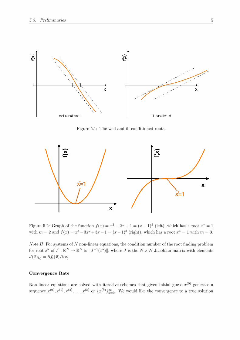
Note I : If f ′ (x∗) = 0, the problem is ill-conditioned. This is the case for roots with multiplicity

m > 1. Thus, roots with multiplicity m > 1 are ill-conditioned. An example of the well and

ill-conditioned root is shown in Figure 5.2.

5.3. Preliminaries 5

Figure 5.1: The well and ill-conditioned roots.

*

*

Figure 5.2: Graph of the function f(x) = x2 − 2x+ 1 = (x− 1)2 (left), which has a root x∗ = 1

with m = 2 and f(x) = x3−3x2 +3x−1 = (x−1)3 (right), which has a root x∗ = 1 with m = 3.

Note II : For systems of N non-linear equations, the condition number of the root finding problem

for root ~x∗ of ~F : RN → RN is ‖J−1(~x∗)‖, where J is the N ×N Jacobian matrix with elements

J(~x)i,j = ∂fi(~x)/∂xj .

Convergence Rate

Non-linear equations are solved with iterative schemes that given initial guess x(0) generate a

sequence x(0), x(1), x(2), . . . , x(k) or {x(k)}∞k=0. We would like the convergence to a true solution

6 Chapter 5. Solving Non-Linear Equations

x∗ to be as fast as possible. The error for x(k) is given by

E(k) = x(k) − x∗ (5.3.4)

If the sequence of {x(k)}∞k=0 converges to x∗ and

limk→∞

|E(k+1)||E(k)|r = C (5.3.5)

we say that the sequence is converging with order r and a rate of convergence/asymptotic error

constant C (C is finite). Common cases according to the value of r:

• r = 1: linear convergence for (0 < C < 1); if C = 0 superlinear; if C = 1 sublinear

• r = 2: quadratic

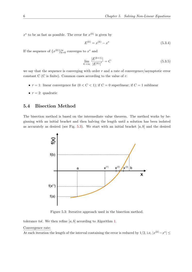
5.4 Bisection Method

The bisection method is based on the intermediate value theorem. The method works by be-

ginning with an initial bracket and then halving the length until a solution has been isolated

as accurately as desired (see Fig. 5.3). We start with an initial bracket [a, b] and the desired

(1)

(1)

(2) (3)x

f(a)

f(b)

f(x )

a bxx

Figure 5.3: Iterative approach used in the bisection method.

tolerance tol. We then refine [a, b] according to Algorithm 1.

Convergence rate:

At each iteration the length of the interval containing the error is reduced by 1/2, i.e, |x(k)−x∗| ≤

5.4. Bisection Method 7

Algorithm 1 Bisection Method

Input:

a, b, {initial interval}tol, {tolerance}kmax, {maximal number of iterations}

Output:

x(k), {approximate solution after k iterations}

Steps:

k ← 1

while (b− a) > tolandk < kmax do

x(k) ← (a+ b)/2

if sign(f(a)) = sign(f(x(k))) then

a← x(k)

else

b← x(k)

end if

k ← k + 1

end while

(b− a)/2k. Taking the worst case error we can write

|E(k+1)||E(k)|r =

2k

2k+1=

1

2. (5.4.1)

Comparing Eq. (5.4.1) with Eq. (5.3.5) we observe that r = 1 and C = 0.5, i.e., the bisection

method converges linearly. In terms of binary numbers, one bit of accuracy is gained in the

approximate solution for each iteration of the bisection method. Given the starting interval

[a, b] after k iterations, the interval is (b − a)/2k, so achieving an error tolerance of tol requires

k = log2((b− a)/tol) steps, regardless of f .

Pros:

• The bisection method is certain to converge.

• The bisection method makes no use of actual function values, only of their signs.

• The function doesn’t need to be differentiable.

Cons:

• The convergence is slow.

• The initial interval needs to be known beforehand

8 Chapter 5. Solving Non-Linear Equations

5.5 Newton’s Method

Assume a function f is differentiable and has a zero at x∗. Furthermore, let x(k−1) be an

approximation to x∗ such that f ′(x(k−1)) 6= 0 and |x∗ − x(k−1)| is small. We can then expand

the function f about x∗ using Taylor series, where we only consider the first two terms as the

|x∗ − x(k−1)| is supposed to be small, i.e.,

0 = f(x∗) ≈ f(x(k−1)) + f ′(x(k−1))(x∗ − x(k−1)). (5.5.1)

Solving the Eq. (5.5.1) for x∗ we get:

x∗ ≈ x(k−1) − f(x(k−1))

f ′(x(k−1))= x(k), (5.5.2)

which is not the true solution since we didn’t keep all of the terms in the Taylor series but it can

be used as the next guess. Given the initial guess x(0) Newton’s method generates a sequence

{x(k)}∞k=0 where

x(k) = x(k−1) − f(x(k−1))

f ′(x(k−1)). (5.5.3)

Graphically the procedure is visualized in Fig. 5.4. Newton’s method approximates the non-linear

function f by the tangent line at f(x(k−1)).

f(x)

x

x*

x(0)x(1)

f(x(0))

x(2)θ

tan(✓) =f(x(0))

x(0) � x(1)= f 0(x(0))

) x(0) � x(1) =f(x(0))

f 0(x(0))

) x(1) = x(0) � f(x(0))

f 0(x(0))

Figure 5.4: Graphical example of Newton iterations as we follow the tangents of f(x).

Convergence rate:

Convergence for simple roots is quadratic. For roots of multiplicity m > 1, the convergence is

linear unless we modify the iteration (Eq. (5.5.3)) to x(k) = x(k−1) −mf(x(k−1))/f ′(x(k−1)).

5.5. Newton’s Method 9

Proof:

f(x∗) = 0 E(k) = x(k) − x∗g(x) = x− f(x)/f ′(x) → g(x∗) = x∗

g(x(k)) = g(x∗ + E(k)) = g(x∗) + g′(x∗)E(k) + 0.5g′′(x∗)(E(k))2 +O((E(k))3)

g(x(k)) = x(k+1) = x∗ + E(k+1)

E(k+1) = g′(x∗)E(k) + 0.5g′′(x∗)(E(k))2 +O((E(k))3)

g′(x) = (x− f(x)/f ′(x))′ = f(x)f ′′(x)/(f ′(x))2 → g′(x∗) = 0

g′(x) = (f(x)f ′′(x)/(f ′(x))2)′ → g′′(x∗) = f ′′(x∗)/f ′(x∗) 6= 0

E(k+1) = 0.5g′′(x∗)(E(k))2 +O((E(k))3)

limk→∞|E(k+1)||E(k)|2

≤ 12g′′(x∗) ≤ |f ′′(x∗)|2f ′(x∗) = C → r = 2

(5.5.4)

Pros:

• Quadratic convergence

Cons:

• The method is not guaranteed to converge. It is sensitive to initial conditions.

• If for some k the f ′(x(k)) = 0 we cannot proceed.

• Newton’s method requires the evaluation of both function and derivative at each iter-

ation.

5.5.1 Secant Method

Evaluating the derivative may be expensive or inconvenient. KEY IDEA: If something is

expensive or inconvenient to compute, replace it with a numerical approximation.

Let

f ′(x(k−1)) =f(x(k−1))− f(x(k−2))

x(k−1) − x(k−2) (5.5.5)

then the method reads as

x(k) = x(k−1) − f(x(k−1))x(k−1) − x(k−2)

f(x(k−1))− f(x(k−2))(5.5.6)

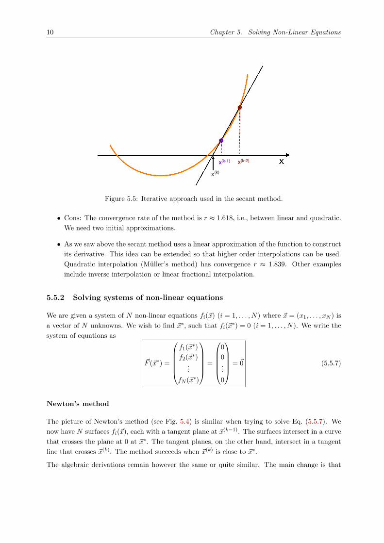
The secant method approximates the non-linear function f by a secant line through previous

two iterations (see Fig. 5.5).

Notes:

• Pros: We avoid the evaluation of the derivative. At each step, we need to perform 1

function evaluation.

10 Chapter 5. Solving Non-Linear Equations

x(k)

(k-1) (k-2)x x

Figure 5.5: Iterative approach used in the secant method.

• Cons: The convergence rate of the method is r ≈ 1.618, i.e., between linear and quadratic.

We need two initial approximations.

• As we saw above the secant method uses a linear approximation of the function to construct

its derivative. This idea can be extended so that higher order interpolations can be used.

Quadratic interpolation (Muller’s method) has convergence r ≈ 1.839. Other examples

include inverse interpolation or linear fractional interpolation.

5.5.2 Solving systems of non-linear equations

We are given a system of N non-linear equations fi(~x) (i = 1, . . . , N) where ~x = (x1, . . . , xN ) is

a vector of N unknowns. We wish to find ~x∗, such that fi(~x∗) = 0 (i = 1, . . . , N). We write the

system of equations as

~F (~x∗) =

f1(~x

∗)

f2(~x∗)

...

fN (~x∗)

=

0

0...

0

= ~0 (5.5.7)

Newton’s method

The picture of Newton’s method (see Fig. 5.4) is similar when trying to solve Eq. (5.5.7). We

now have N surfaces fi(~x), each with a tangent plane at ~x(k−1). The surfaces intersect in a curve

that crosses the plane at 0 at ~x∗. The tangent planes, on the other hand, intersect in a tangent

line that crosses ~x(k). The method succeeds when ~x(k) is close to ~x∗.

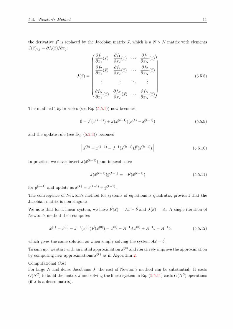
The algebraic derivations remain however the same or quite similar. The main change is that

5.5. Newton’s Method 11

the derivative f ′ is replaced by the Jacobian matrix J , which is a N ×N matrix with elements

J(~x)i,j = ∂fi(~x)/∂xj :

J(~x) =

∂f1∂x1

(~x)∂f1∂x2

(~x) · · · ∂f1∂xN

(~x)

∂f2∂x1

(~x)∂f2∂x2

(~x) · · · ∂f2∂xN

(~x)

......

. . ....

∂fN∂x1

(~x)∂fN∂x2

(~x) · · · ∂fN∂xN

(~x)

(5.5.8)

The modified Taylor series (see Eq. (5.5.1)) now becomes

~0 = ~F (~x(k−1)) + J(~x(k−1))(~x(k) − ~x(k−1)) (5.5.9)

and the update rule (see Eq. (5.5.3)) becomes

~x(k) = ~x(k−1) − J−1(~x(k−1))~F (~x(k−1)) (5.5.10)

In practice, we never invert J(~x(k−1)) and instead solve

J(~x(k−1))~y(k−1) = −~F (~x(k−1)) (5.5.11)

for ~y(k−1) and update as ~x(k) = ~x(k−1) + ~y(k−1).

The convergence of Newton’s method for systems of equations is quadratic, provided that the

Jacobian matrix is non-singular.

We note that for a linear system, we have ~F (~x) = A~x −~b and J(~x) = A. A single iteration of

Newton’s method then computes

~x(1) = ~x(0) − J−1(~x(0))~F (~x(0)) = ~x(0) −A−1A~x(0) +A−1b = A−1b, (5.5.12)

which gives the same solution as when simply solving the system A~x = ~b.

To sum up: we start with an initial approximation ~x(0) and iteratively improve the approximation

by computing new approximations ~x(k) as in Algorithm 2.

Computational Cost

For large N and dense Jacobians J , the cost of Newton’s method can be substantial. It costs

O(N2) to build the matrix J and solving the linear system in Eq. (5.5.11) costs O(N3) operations

(if J is a dense matrix).

12 Chapter 5. Solving Non-Linear Equations

Algorithm 2 Newton’s method

Input:

~x(0), {vector of length N with initial approximation}tol, {tolerance: stop if ‖~x(k) − ~x(k−1)‖ < tol}kmax, {maximal number of iterations: stop if k > kmax}

Output:

~x(k), {solution of ~F (~x(k)) = ~0 within tolerance tol} (or a message if k > kmax reached)

Steps:

k ← 1

while k ≤ kmax do

Calculate ~F (~x(k−1)) and N ×N matrix J(~x(k−1))

Solve the N ×N linear system J(~x(k−1))~y = −~F (~x(k−1))

~x(k) ← ~x(k−1) + ~y

if ‖~y‖ < tol then

break

end if

k ← k + 1

end while

Secant Method

Reduce the cost of Newton’s Method by:

• using function values at successive iterations to build approximate Jacobians and avoid

explicit evaluations of the derivatives (note that this is also necessary if for some reason

you cannot evaluate the derivatives analytically)

• update factorization (to solve the linear system) of approximate Jacobians rather than

refactoring it each iteration

Modified Newton Method

The simplest approach is to keep J fixed during the iterations of Newton’s method. So instead of

updating or recomputing J , we compute J (0) = J(x(0)) once and (instead of Eq. (5.5.11)) solve

J (0)~y(k−1) = −~F (~x(k−1)). (5.5.13)

This can be done efficiently by performing a LU decomposition of J (0) once and use it over and

over again for different ~F (~x(k−1)). This removes the O(N3) cost of solving the linear system. We

only have to evaluate ~F (~x(k−1)) and can then compute ~y(k−1) in O(N2) operations. This method

can only succeed if J is not changing rapidly.

5.5. Newton’s Method 13

Quasi Newton Method

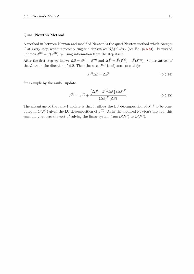
A method in between Newton and modified Newton is the quasi Newton method which changes

J at every step without recomputing the derivatives ∂fi(~x)/∂xj (see Eq. (5.5.8)). It instead

updates J (0) = J(x(0)) by using information from the step itself.

After the first step we know: ∆~x = ~x(1) − ~x(0) and ∆~F = ~F (~x(1)) − ~F (~x(0)). So derivatives of

the fi are in the direction of ∆~x. Then the next J (1) is adjusted to satisfy:

J (1)∆~x = ∆~F (5.5.14)

for example by the rank-1 update

J (1) = J (0) +

(∆~F − J (0)∆~x

)(∆~x)T

(∆~x)T (∆~x). (5.5.15)

The advantage of the rank-1 update is that it allows the LU decomposition of J (1) to be com-

puted in O(N2) given the LU decomposition of J (0). As in the modified Newton’s method, this

essentially reduces the cost of solving the linear system from O(N3) to O(N2).