ModelPredictiveControl: ARisingTechnology

CCTA2020

Model Predictive Control:A Rising Technologyin the Automotive Industry

Alberto Bemporad

http://imt.lu/ab

Outline

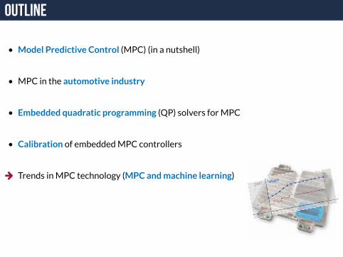
• Model Predictive Control (MPC) (in a nutshell)

• MPC in the automotive industry

• Embedded quadratic programming (QP) solvers forMPC

• Calibration of embeddedMPC controllers

• Trends inMPC technology (MPC andmachine learning)

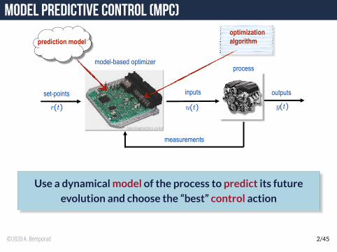
Model Predictive Control (MPC)

prediction model

model-based optimizer

set-points outputsinputs

measurements

r(t) u(t) y(t)

optimization

algorithm

process

(aecdiagnostics.com)

Use a dynamical model of the process to predict its future

evolution and choose the “best” control action

©2020 A. Bemporad 2/45

t+1 t+1+k t+N+1

future

predicted outputs

manipulated inputs

t t+k t+N

uk

r(t)

yk

past

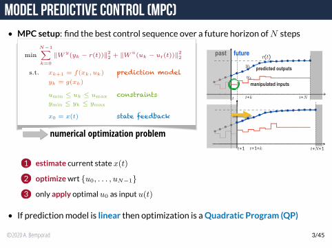
Model Predictive Control (MPC)• MPC setup: find the best control sequence over a future horizon ofN steps

min

N−1∑

k=0

∥Wy(yk − r(t))∥

22 + ∥W

u(uk − ur(t))∥

22

s.t. xk+1 = f(xk, uk) prediction modelyk = g(xk)

umin ≤ uk ≤ umax constraintsymin ≤ yk ≤ ymax

x0 = x(t) state feedback

numerical optimization problem

1 estimate current state x(t)

2 optimizewrt {u0, . . . , uN−1}

3 only apply optimal u0 as input u(t)

• If predictionmodel is linear then optimization is aQuadratic Program (QP)


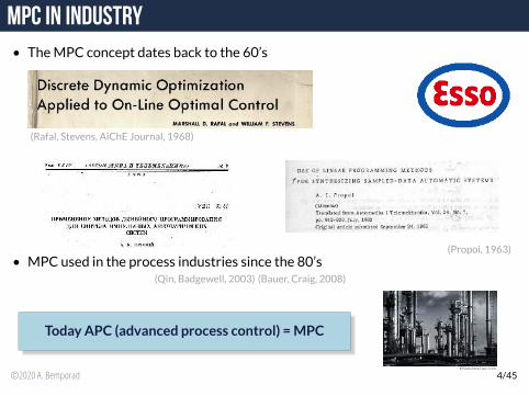
MPC in industry• TheMPC concept dates back to the 60’s

3

(Rafal, Stevens, AiChE Journal, 1968)

(Propoi, 1963)• MPC used in the process industries since the 80’s

(Qin, Badgewell, 2003) (Bauer, Craig, 2008)

Today APC (advanced process control) =MPC

©SimulateLive.com


Outline


MPC in the automotive industry




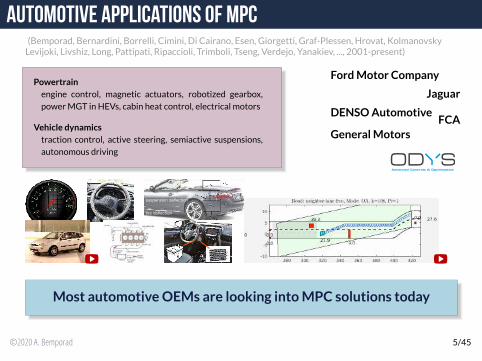
Automotive applications of MPC(Bemporad, Bernardini, Borrelli, Cimini, Di Cairano, Esen, Giorgetti, Graf-Plessen, Hrovat, KolmanovskyLevijoki, Livshiz, Long, Pattipati, Ripaccioli, Trimboli, Tseng, Verdejo, Yanakiev, ..., 2001-present)

Powertrainengine control, magnetic actuators, robotized gearbox,

powerMGT in HEVs, cabin heat control, electrical motors

Vehicle dynamicstraction control, active steering, semiactive suspensions,

autonomous driving

FordMotor Company

Jaguar

DENSOAutomotiveFCA

GeneralMotors

4

tire deflection

suspension deflection

4

tire deflection

suspension deflection

Most automotiveOEMs are looking intoMPC solutions today


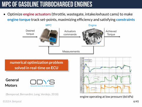
MPC of gasoline turbocharged engines• Optimize engine actuators (throttle, wastegate, intake/exhaust cams) tomake

engine torque track set-points, maximizing efficiency and satisfying constraints

Measurements

Desired

torqueActuators

commands

Achieved

Torque

EngineMPC

numerical optimization problem

solved in real-time on ECU

General

Motors

(Bemporad, Bernardini, Long, Verdejo, 2018)engine operating at low pressure (66 kPa)


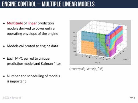
Engine control – Multiple linear models

• Multitude of linear prediction

models derived to cover entire

operating envelope of the engine

• Models calibrated to engine data

• EachMPC paired to unique

predictionmodel and Kalman filter

• Number and scheduling of models

is important

(courtesy of J. Verdejo, GM)


yr1

Desired

Torqueur1 throttle

ur2 wg

ur3 ecam

ur4 icam

(courtesy of J. Verdejo, GM)

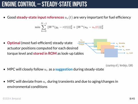
Engine control – Steady-state inputs

• Good steady-state input references ur(t) are very important for fuel efficiency

min

N−1∑

k=0

∥W y(yk − r(t))∥22 + ∥Wu(uk − ur(t))∥22

• Optimal (most fuel-efficient) steady-state

actuator positions computed for each desired

torque level and stored in ROM as look-up tables

• MPCwill closely follow ur as a suggestion during steady-state

• MPCwill deviate from ur during transients and due to aging/changes in

environmental conditions


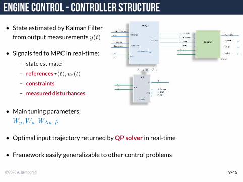
Engine control - Controller structure

• State estimated by Kalman Filter

from output measurements y(t)

• Signals fed toMPC in real-time:

– state estimate

– references r(t), ur(t)

– constraints

– measured disturbances

• Main tuning parameters:

Wy,Wu,W∆u, ρ

• Optimal input trajectory returned byQP solver in real-time

• Framework easily generalizable to other control problems


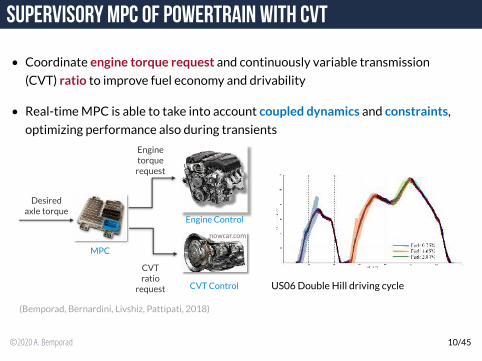
Supervisory MPC of powertrain with CVT

• Coordinate engine torque request and continuously variable transmission

(CVT) ratio to improve fuel economy and drivability

• Real-timeMPC is able to take into account coupled dynamics and constraints,

optimizing performance also during transients

CVT Control

Desired

axle torque

MPC

Engine Control

Engine

torque

request

CVT

ratio

request

nowcar.com

(Bemporad, Bernardini, Livshiz, Pattipati, 2018)

US06Double Hill driving cycle

©2020 A. Bemporad 10/45

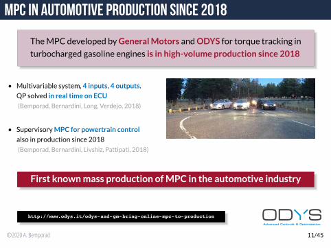
MPC in automotive production since 2018

TheMPCdeveloped byGeneralMotors andODYS for torque tracking in

turbocharged gasoline engines is in high-volume production since 2018

• Multivariable system, 4 inputs, 4 outputs.

QP solved in real time on ECU

(Bemporad, Bernardini, Long, Verdejo, 2018)

• SupervisoryMPC for powertrain control

also in production since 2018

(Bemporad, Bernardini, Livshiz, Pattipati, 2018)

First knownmass production ofMPC in the automotive industry

http://www.odys.it/odys-and-gm-bring-online-mpc-to-production

©2020 A. Bemporad 11/45

controller

desired

torque

torqueactuators

sensors

engine


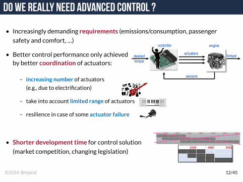
Do we really need advanced control ?

• Increasingly demanding requirements (emissions/consumption, passenger

safety and comfort, …)

• Better control performance only achievedby better coordination of actuators:

– increasing number of actuators

(e.g., due to electrification)

– take into account limited range of actuators

– resilience in case of some actuator failure

• Shorter development time for control solution

(market competition, changing legislation)

©2020 A. Bemporad 12/45

u1

u1 max

u1 min

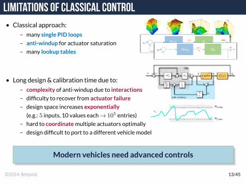
Limitations of classical control• Classical approach:

– many single PID loops

– anti-windup for actuator saturation

– many lookup tables

• Long design & calibration time due to:

– complexity of anti-windup due to interactions

– difficulty to recover from actuator failure

– design space increases exponentially

(e.g.: 5 inputs, 10 values each→ 105 entries)

– hard to coordinatemultiple actuators optimally

– design difficult to port to a different vehicle model

Modern vehicles need advanced controls

©2020 A. Bemporad 13/45

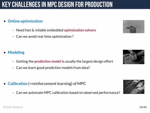
Key challenges in MPC design for production

• Online optimization

– Need fast & reliable embedded optimization solvers

– Canwe avoid real-time optimization ?

• Modeling

– Getting the predictionmodel is usually the largest design effort

– Canwe learn good predictionmodels from data?

• Calibration (=reinforcement learning) ofMPC

– Canwe automateMPC calibration based on observed performance?

©2020 A. Bemporad 14/45

Outline



Embedded quadratic programming (QP) solvers forMPC



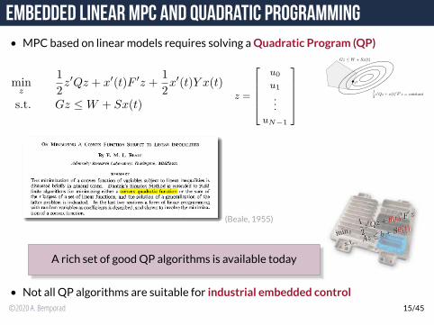
Embedded Linear MPC and Quadratic Programming• MPC based on linear models requires solving aQuadratic Program (QP)

minz

1

2z′Qz + x′(t)F ′z +

1

2x′(t)Y x(t)

s.t. Gz ≤ W + Sx(t)z =

u0

u1

...

uN−1

z*

(Beale, 1955)

A rich set of goodQP algorithms is available today

• Not all QP algorithms are suitable for industrial embedded control©2020 A. Bemporad 15/45

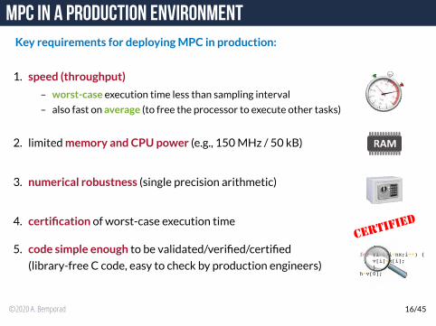
MPC in a production environmentKey requirements for deployingMPC in production:

1. speed (throughput)

– worst-case execution time less than sampling interval

– also fast on average (to free the processor to execute other tasks)

2. limitedmemory and CPU power (e.g., 150MHz / 50 kB)

3. numerical robustness (single precision arithmetic)

4. certification of worst-case execution time

5. code simple enough to be validated/verified/certified

(library-free C code, easy to check by production engineers)for (i=0;i<nx;i++) {

v[i]=x[i];

}

h=v[0];

©2020 A. Bemporad 16/45

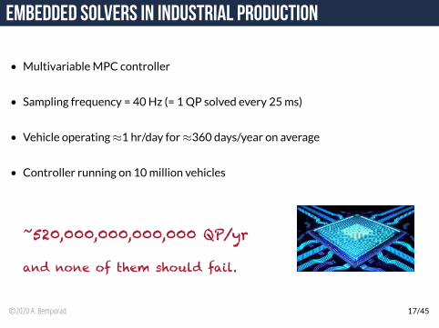
Embedded solvers in industrial production

• MultivariableMPC controller

• Sampling frequency = 40Hz (= 1QP solved every 25ms)

• Vehicle operating≈1 hr/day for≈360 days/year on average

• Controller running on 10million vehicles

~520,000,000,000,000 QP/yrand none of them should fail.

©2020 A. Bemporad 17/45

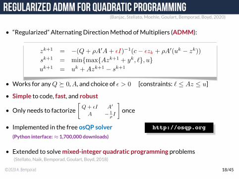
Regularized ADMM for quadratic programming(Banjac, Stellato, Moehle, Goulart, Bemporad, Boyd, 2020)

• “Regularized” Alternating DirectionMethod ofMultipliers (ADMM):

zk+1 = −(Q+ ρA′A+ ϵI)−1(c− ϵzk + ρA′(uk − zk))

sk+1 = min{max{Azk+1 + yk, ℓ}, u}

uk+1 = uk +Azk+1 − sk+1

• Works for anyQ ≽ 0,A, and choice of ϵ > 0 [constraints: ℓ ≤ Az ≤ u]

• Simple to code, fast, and robust

• Only needs to factorize

[Q+ ϵI A′

A − 1

ρI

]

once

• Implemented in the free osQP solver http://osqp.org(Python interface:≈ 1,700,000 downloads)

• Extended to solvemixed-integer quadratic programming problems(Stellato, Naik, Bemporad, Goulart, Boyd, 2018)

©2020 A. Bemporad 18/45

Solving QP’s via nonnegative least squares(Bemporad, 2016)

• Complete the squares and transformQP to least distance problem (LDP)

minz

12z

′Qz + c′z

s.t. Gz ≤ g

Q = Q′ ≻ 0

Q = L′L

u , Lz + L−T c

minu

12∥u∥

2

s.t. Mu ≤ d

• An LDP is equivalent to the nonnegative least squares (NNLS) problem

(Lawson, Hanson, 1974)

miny

1

2

∥∥∥∥∥

[

M ′

d′

]

y +

[

0

1

]∥∥∥∥∥

2

2

s.t. y ≥ 0

M = GL−1

d = b+GQ−1c

• If residual= 0 then the original QP is infeasible. Otherwise set

z∗ = −1

1 + d′y∗L−1M ′y∗ −Q−1c

©2020 A. Bemporad 19/45

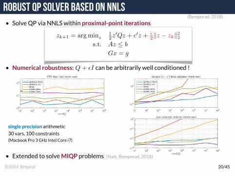
Robust QP solver based on NNLS(Bemporad, 2018)

• SolveQP via NNLSwithin proximal-point iterations

zk+1 = argminz12z

′Qz + c′z + ϵ2∥z − zk∥

22

s.t. Az ≤ b

Gx = g

• Numerical robustness: Q+ ϵI can be arbitrarily well conditioned !

single precision arithmetic

30 vars, 100 constraints(Macbook Pro 3 GHz Intel Core i7)

• Extended to solveMIQP problems (Naik, Bemporad, 2018)

©2020 A. Bemporad 20/45

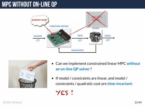
MPC without on-line QP

prediction model



measurements

r(t) u(t) y(t)

optimization

algorithm

process


• Canwe implement constrained linearMPCwithout

an on-lineQP solver ?

• If model / constraints are linear, andmodel /

constraints / quadratic cost are time-invariant:

YES !

©2020 A. Bemporad 21/45

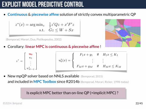
Explicit model predictive control• Continuous& piecewise affine solution of strictly convexmultiparametric QP

z∗(x) = argminz12z

′Qz + x′F ′z

s.t. Gz ≤ W + Sx

(Bemporad,Morari, Dua, Pistikopoulos, 2002)

• Corollary: linearMPC is continuous & piecewise affine !

z∗

=

u0

u1

.

.

.

u∗

N−1

u∗

0(x) =

F1x+ g1 if H1x ≤ K1

......

FMx+ gM if HMx ≤ KM

• NewmpQP solver based onNNLS available (Bemporad, 2015)

and included inMPCToolbox since R2014b (Bemporad,Morari, Ricker, 1998-today)

Is explicit MPC better than on-line QP (=implicit MPC) ?

©2020 A. Bemporad 22/45

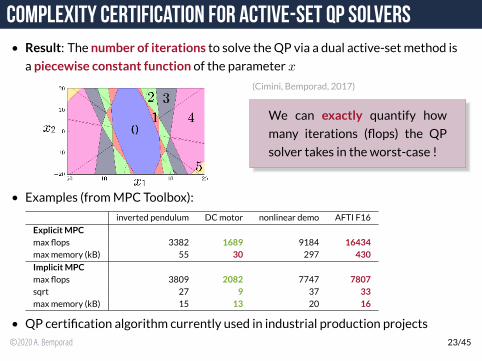
Complexity certification for active-set QP solvers• Result: The number of iterations to solve theQP via a dual active-set method is

a piecewise constant function of the parameter x

(Cimini, Bemporad, 2017)

We can exactly quantify how

many iterations (flops) the QP

solver takes in the worst-case !

• Examples (fromMPC Toolbox):

inverted pendulum DCmotor nonlinear demo AFTI F16

ExplicitMPCmax flops 3382 1689 9184 16434maxmemory (kB) 55 30 297 430

ImplicitMPCmax flops 3809 2082 7747 7807sqrt 27 9 37 33maxmemory (kB) 15 13 20 16

• QP certification algorithm currently used in industrial production projects

©2020 A. Bemporad 23/45

Outline




Calibration of embeddedMPC controllers


x1

x3

x2

x4

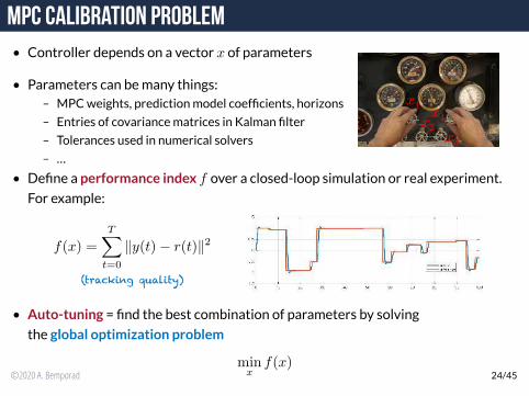
MPC calibration problem• Controller depends on a vector x of parameters

• Parameters can bemany things:– MPCweights, predictionmodel coefficients, horizons

– Entries of covariancematrices in Kalman filter

– Tolerances used in numerical solvers

– …

• Define a performance index f over a closed-loop simulation or real experiment.

For example:

f(x) =

T∑

t=0

∥y(t)− r(t)∥2

(tracking quality)

• Auto-tuning = find the best combination of parameters by solving

the global optimization problem

minx

f(x)©2020 A. Bemporad 24/45

Global optimization algorithms for auto-tuning

What is a good optimization algorithm to solvemin f(x) ?

• The algorithm should not require the gradient∇f of f(x)

(derivative-free or black-box optimization )

• The algorithm should not get stuck on local minima (global optimization)

• The algorithm shouldmake the fewest evaluations of the cost function f

(which is expensive to evaluate)

©2020 A. Bemporad 25/45

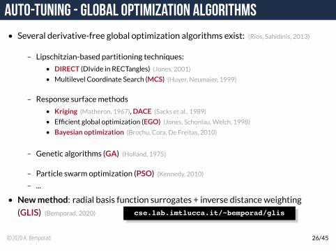
Auto-tuning - Global optimization algorithms

• Several derivative-free global optimization algorithms exist: (Rios, Sahidinis, 2013)

– Lipschitzian-based partitioning techniques:

• DIRECT (DIvide in RECTangles) (Jones, 2001)

• Multilevel Coordinate Search (MCS) (Huyer, Neumaier, 1999)

– Response surfacemethods

• Kriging (Matheron, 1967),DACE (Sacks et al., 1989)

• Efficient global optimization (EGO) (Jones, Schonlau,Welch, 1998)

• Bayesian optimization (Brochu, Cora, De Freitas, 2010)

– Genetic algorithms (GA) (Holland, 1975)

– Particle swarm optimization (PSO) (Kennedy, 2010)

– ...

• Newmethod: radial basis function surrogates + inverse distance weighting

(GLIS) (Bemporad, 2020) cse.lab.imtlucca.it/~bemporad/glis

©2020 A. Bemporad 26/45

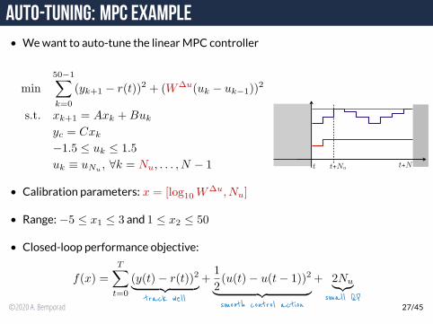
t t+Nu t+N

Auto-tuning: MPC example• Wewant to auto-tune the linearMPC controller

min

50−1∑

k=0

(yk+1 − r(t))2 + (W∆u(uk − uk−1))2

s.t. xk+1 = Axk +Buk

yc = Cxk

−1.5 ≤ uk ≤ 1.5

uk ≡ uNu, ∀k = Nu, . . . , N − 1

• Calibration parameters: x = [log10 W∆u, Nu]

• Range: −5 ≤ x1 ≤ 3 and 1 ≤ x2 ≤ 50

• Closed-loop performance objective:

f(x) =

T∑

t=0

(y(t)− r(t))2︸︷︷︸

track well

+1

2(u(t)− u(t− 1))2

︸︷︷︸

smooth control action

+ 2Nu︸︷︷︸

small QP©2020 A. Bemporad 27/45

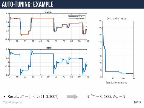
Auto-tuning: Example

0 10 20 30 40 50 60 70 80 90 100-1.5

-1

-0.5

0

0.5

1

1.5output

outputreference

0 10 20 30 40 50 60 70 80 90 100-1.5

-1

-0.5

0

0.5

1

1.5input

best function value

0 50 100 15060

80

100

120

140

160

180

200

220

function evaluations

• Result: x⋆ = [−0.2341, 2.3007] W∆u = 0.5833,Nu = 2

©2020 A. Bemporad 28/45

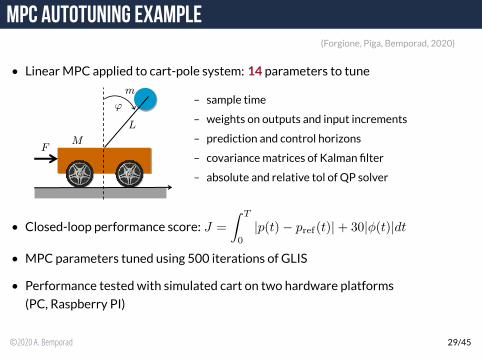
MPC Autotuning Example(Forgione, Piga, Bemporad, 2020)

• LinearMPC applied to cart-pole system: 14 parameters to tune

L

m

'

MF

– sample time

– weights on outputs and input increments

– prediction and control horizons

– covariancematrices of Kalman filter

– absolute and relative tol of QP solver

• Closed-loop performance score: J =

∫ T

0

|p(t)− pref(t)|+ 30|ϕ(t)|dt

• MPC parameters tuned using 500 iterations of GLIS

• Performance tested with simulated cart on two hardware platforms

(PC, Raspberry PI)

©2020 A. Bemporad 29/45

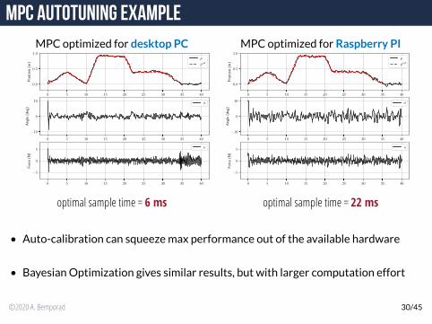
MPC Autotuning ExampleMPCoptimized for desktop PC MPC optimized forRaspberry PI

0 5 10 15 20 25 30 35 40

0.0

0.5

1.0

Position(m

)

p

pref

0 5 10 15 20 25 30 35 40

−10

0

10

Angle

(deg)

φ

0 5 10 15 20 25 30 35 40

−5

0

5

Force

(N)

u

0 5 10 15 20 25 30 35 40

0.0

0.5

1.0

Position(m

)

p

pref

0 5 10 15 20 25 30 35 40

−10

0

10

Angle

(deg)

φ

0 5 10 15 20 25 30 35 40

−5

0

5

Force

(N)

u

optimal sample time = 6 ms optimal sample time = 22 ms

• Auto-calibration can squeezemax performance out of the available hardware

• BayesianOptimization gives similar results, but with larger computation effort

©2020 A. Bemporad 30/45

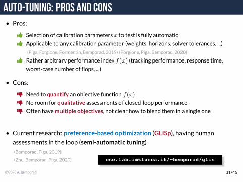
Auto-tuning: Pros and Cons• Pros:

Selection of calibration parameters x to test is fully automatic

Applicable to any calibration parameter (weights, horizons, solver tolerances, ...)

(Piga, Forgione, Formentin, Bemporad, 2019) (Forgione, Piga, Bemporad, 2020)

Rather arbitrary performance index f(x) (tracking performance, response time,

worst-case number of flops, ...)

• Cons:

Need to quantify an objective function f(x)

No room for qualitative assessments of closed-loop performance

Often havemultiple objectives, not clear how to blend them in a single one

• Current research: preference-based optimization (GLISp), having human

assessments in the loop (semi-automatic tuning)

(Bemporad, Piga, 2019)

(Zhu, Bemporad, Piga, 2020) cse.lab.imtlucca.it/~bemporad/glis

©2020 A. Bemporad 31/45

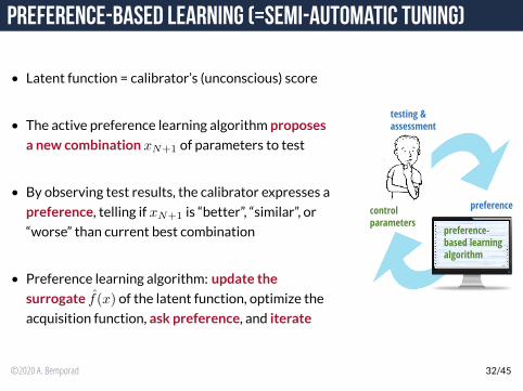
Preference-based Learning (=Semi-automatic tuning)

• Latent function = calibrator’s (unconscious) score

• The active preference learning algorithm proposes

a new combination xN+1 of parameters to test

• By observing test results, the calibrator expresses a

preference, telling if xN+1 is “better”, “similar”, or

“worse” than current best combination

• Preference learning algorithm: update the

surrogate f(x) of the latent function, optimize the

acquisition function, ask preference, and iterate

controlparameters

testing &assessment

preference

preference-based learning algorithm

©2020 A. Bemporad 32/45

0 10 20 30 40 50 60 70 80 90 100-1.5

-1

-0.5

0

0.5

1

1.5output

outputreference

0 10 20 30 40 50 60 70 80 90 100-2

-1

0

1

2input

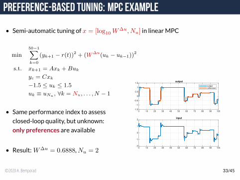
Preference-based tuning: MPC example

• Semi-automatic tuning of x = [log10 W∆u, Nu] in linearMPC

min

50−1∑

k=0

(yk+1 − r(t))2 + (W∆u(uk − uk−1))2

s.t. xk+1 = Axk +Buk

yc = Cxk

−1.5 ≤ uk ≤ 1.5

uk ≡ uNu , ∀k = Nu, . . . , N − 1

• Same performance index to assess

closed-loop quality, but unknown:

only preferences are available

• Result:W∆u = 0.6888,Nu = 2

©2020 A. Bemporad 33/45

Outline





Trends inMPC technology (MPC andmachine learning)

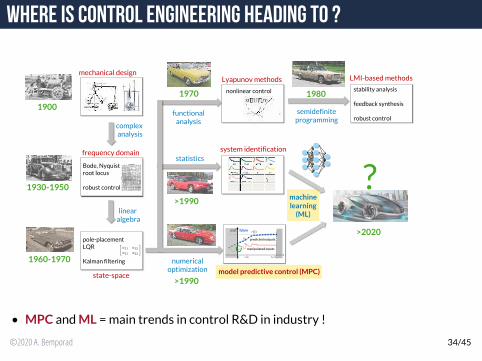
Where is control engineering heading to ?

\

mechanical design

frequency domain

Bode, Nyquist

root locus

robust control

complex

analysis

state-space

pole-placement

LQR

Kalman filtering

linear

algebra

Lyapunov methods

functional

analysis

nonlinear control

semidefinite

programming

statistics

LMI-based methods

stability analysis

feedback synthesis

robust control

system identification

model predictive control (MPC)

numerical

optimization

machinelearning

(ML)

?

future

predicted outputs

manipulated inputs

t t+k t+N

uk

r(t)

yk

past

1900

1930-1950

1960-1970

1970

>1990

>1990

1980

>2020

• MPC andML =main trends in control R&D in industry !

©2020 A. Bemporad 34/45

input

output

Machine Learning (ML)

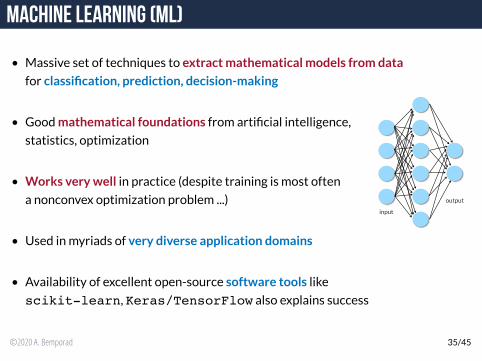
• Massive set of techniques to extract mathematical models from data

for classification, prediction, decision-making

• Goodmathematical foundations from artificial intelligence,

statistics, optimization

• Works verywell in practice (despite training is most often

a nonconvex optimization problem ...)

• Used inmyriads of very diverse application domains

• Availability of excellent open-source software tools like

scikit-learn, Keras/TensorFlow also explains success

©2020 A. Bemporad 35/45

ML for MPC

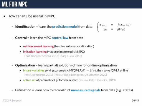
• How canML be useful inMPC:

– Identification = learn the predictionmodel from data

{

xk+1 = f(xk, uk)

yk = g(xk)

– Control = learn theMPC control law from data

• reinforcement learning (best for automatic calibration)

• imitation learning (= approximate explicit MPC)

(Lenz, Knepper, Saxena, 2015) (Karg, Lucia, 2018)

– Optimization = learn (partial) solutions offline for on-line optimization

• binary variables solving parametricMIQP/LP, δ∗ = δ(x), then solveQP/LP online

(Masti, Bemporad, 2019) (Masti, Pippia, Bemporad, De Schutter, 2020)

• active set of parametric QP for warm start (Klauco, Kalúz, Kvasnica, 2019)

– Estimation = learn how to reconstruct unmeasured signals from data (e.g., states)

©2020 A. Bemporad 36/45

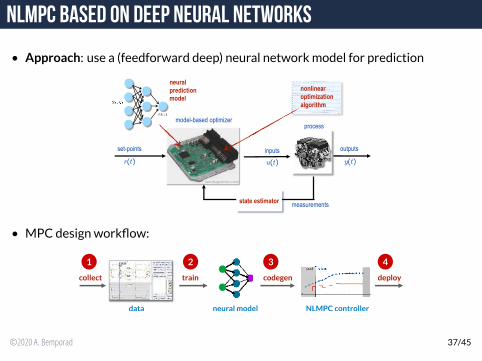
NLMPC based on Deep Neural Networks

• Approach: use a (feedforward deep) neural networkmodel for prediction



measurements

r(t) u(t) y(t)

nonlinear

optimization

algorithm

process

state estimator

neural

prediction

model


• MPC design workflow:

data neural model

collect train codegen

NLMPC controller

deploy

1 2 3 4

©2020 A. Bemporad 37/45

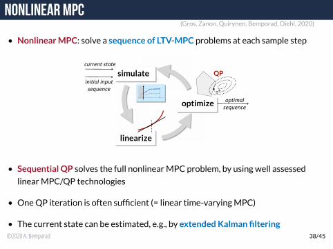
Nonlinear MPC(Gros, Zanon, Quirynen, Bemporad, Diehl, 2020)

• NonlinearMPC: solve a sequence of LTV-MPC problems at each sample step

z*

optimal

sequence

initial input

sequence

QP

current state

linearize

optimize

simulate

• Sequential QP solves the full nonlinearMPC problem, by using well assessed

linearMPC/QP technologies

• OneQP iteration is often sufficient (= linear time-varyingMPC)

• The current state can be estimated, e.g., by extended Kalman filtering©2020 A. Bemporad 38/45

odys.it/embedded-mpc

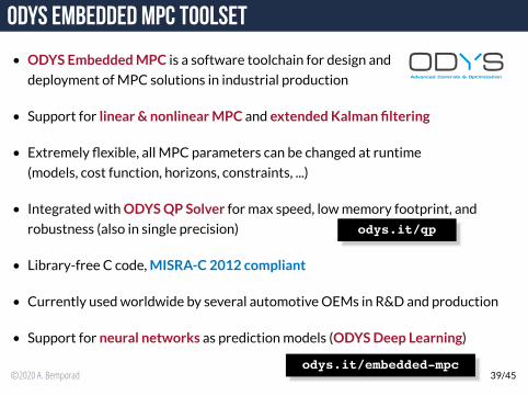
ODYS Embedded MPC Toolset

• ODYS EmbeddedMPC is a software toolchain for design and

deployment ofMPC solutions in industrial production

• Support for linear & nonlinearMPC and extended Kalman filtering

• Extremely flexible, all MPC parameters can be changed at runtime

(models, cost function, horizons, constraints, ...)

• Integrated withODYSQP Solver for max speed, lowmemory footprint, and

robustness (also in single precision) odys.it/qp

• Library-free C code,MISRA-C 2012 compliant

• Currently usedworldwide by several automotiveOEMs in R&D and production

• Support for neural networks as predictionmodels (ODYSDeep Learning)

©2020 A. Bemporad 39/45

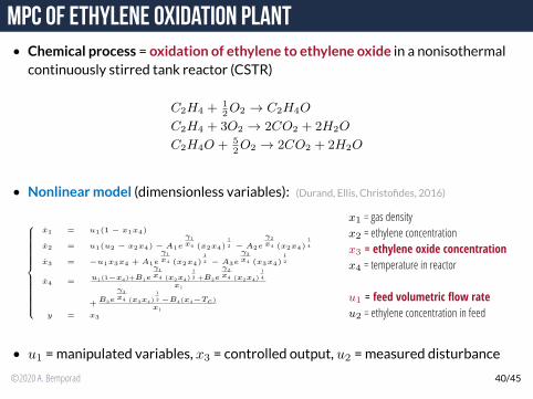
MPC of Ethylene Oxidation Plant• Chemical process = oxidation of ethylene to ethylene oxide in a nonisothermalcontinuously stirred tank reactor (CSTR)

C2H4 +1

2O2 → C2H4O

C2H4 + 3O2 → 2CO2 + 2H2O

C2H4O + 5

2O2 → 2CO2 + 2H2O

• Nonlinearmodel (dimensionless variables): (Durand, Ellis, Christofides, 2016)

x1 = u1(1 − x1x4)

x2 = u1(u2 − x2x4) − A1e

γ1

x4 (x2x4)1

2 − A2e

γ2

x4 (x2x4)1

4

x3 = −u1x3x4 + A1e

γ1

x4 (x2x4)1

2 − A3e

γ3

x4 (x3x4)1

2

x4 =u1(1−x4)+B1e

γ1

x4 (x2x4)

1

2 +B2e

γ2

x4 (x2x4)

1

4

x1

+B3e

γ3

x4 (x3x4)

1

2 −B4(x4−Tc)

x1

y = x3

x1 = gas densityx2 = ethylene concentrationx3 = ethylene oxide concentrationx4 = temperature in reactor

u1 = feed volumetric flow rateu2 = ethylene concentration in feed

• u1 =manipulated variables, x3 = controlled output, u2 =measured disturbance

©2020 A. Bemporad 40/45

MPC of Ethylene Oxidation Plant

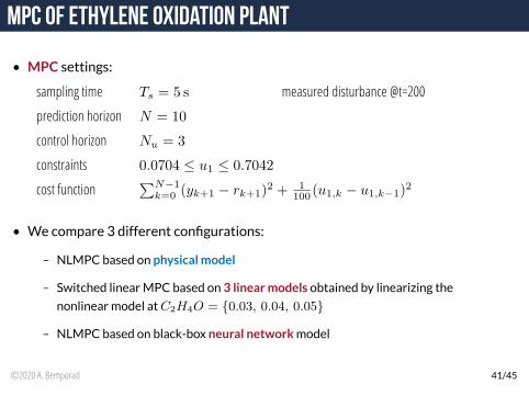
• MPC settings:

sampling time Ts = 5 s measured disturbance @t=200

prediction horizon N = 10

control horizon Nu = 3

constraints 0.0704 ≤ u1 ≤ 0.7042

cost function∑N−1

k=0 (yk+1 − rk+1)2 + 1

100 (u1,k − u1,k−1)2

• We compare 3 different configurations:

– NLMPC based on physical model

– Switched linearMPC based on 3 linearmodels obtained by linearizing the

nonlinear model atC2H4O = {0.03, 0.04, 0.05}

– NLMPC based on black-box neural networkmodel

©2020 A. Bemporad 41/45

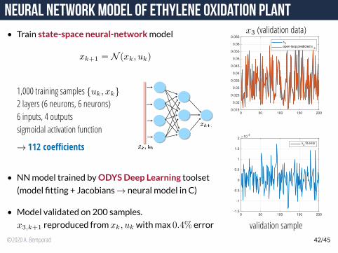
Neural Network Model of Ethylene Oxidation Plant• Train state-space neural-networkmodel

xk+1 = N (xk, uk)

1,000 training samples {uk, xk}

2 layers (6 neurons, 6 neurons)6 inputs, 4 outputssigmoidal activation function

→ 112 coefficients

• NNmodel trained byODYSDeep Learning toolset

(model fitting + Jacobians→ neural model in C)

• Model validated on 200 samples.

x3,k+1 reproduced fromxk, uk withmax 0.4% error

x3 (validation data)

0 50 100 150 2000.015

0.02

0.025

0.03

0.035

0.04

0.045

0.05

0.055

0.06

0.065

x3

open-loop predicted x3

0 50 100 150 200-1.5

-1

-0.5

0

0.5

1

1.5

210

-4

x3 fit error

validation sample©2020 A. Bemporad 42/45

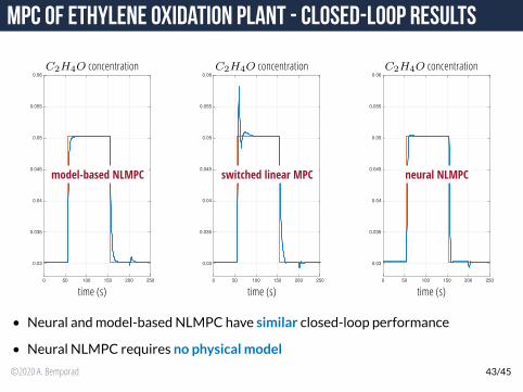
MPC of Ethylene Oxidation Plant - Closed-loop results

C2H4O concentration

0 50 100 150 200 250

0.03

0.035

0.04

0.045

0.05

0.055

0.06

time (s)

model-based NLMPC

C2H4O concentration

0 50 100 150 200 250

0.03

0.035

0.04

0.045

0.05

0.055

0.06

time (s)

switched linear MPC

C2H4O concentration

0 50 100 150 200 250

0.03

0.035

0.04

0.045

0.05

0.055

0.06

time (s)

neural NLMPC

• Neural andmodel-based NLMPC have similar closed-loop performance

• Neural NLMPC requires no physical model

©2020 A. Bemporad 43/45

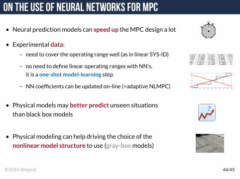
On the use of neural networks for MPC

• Neural predictionmodels can speed up theMPC design a lot

• Experimental data:

– need to cover the operating rangewell (as in linear SYS-ID)

– no need to define linear operating ranges with NN’s,

it is a one-shotmodel-learning step

– NN coefficients can be updated on-line (=adaptive NLMPC)

• Physical models may better predict unseen situations

than black boxmodels

• Physical modeling can help driving the choice of the

nonlinearmodel structure to use (gray-boxmodels)

©2020 A. Bemporad 44/45

Conclusions

• Long history of success ofMPC in the process industries

– multivariable, linear/nonlinear/stochastic systemsw/ constraints

– intuitive to design and calibrate, easy to reconfigure

• MPC is now a viable technology in the automotive industry too:

1. modern ECUs can solveMPC problems in real-time

2. advanced software tools are available for identification, design, calibration, and

deployment ofMPC solutions

3. increasingly tight requirements ask for advancedmultivariable control solutions

4. productionmanagers are willing to deployMPC in the vehicle

• MPC based on deep neural models is probably the next step inMPC technology

©2020 A. Bemporad 45/45

Documents

ModelPredictiveControl: ARisingTechnology