MODELO PARA A FORMATAÇÃO DOS ARTIGOS A SEREM … · Licensed under a Creative Commons Attribution 3.0 United States License [ INDEPENDENT JOURNAL OF MANAGEMENT

INDEPENDENT JOURNAL OF MANAGEMENT & PRODUCTION (IJM&P) http://www.ijmp.jor.br v. 7, n. 1, January - March 2016 ISSN: 2236-269X DOI: 10.14807/ijmp.v7i1.324

[http://creativecommons.org/licenses/by/3.0/us/]

Licensed under a Creative Commons Attribution 3.0 United States License

226

COVARIANCE STABILITY AND THE 2008 FINANCIAL CRISIS: THE IMPACT IN THE PORTFOLIO OF THE 10 BIGGEST

COMPANIES IN BM&FBOVESPA BETWEEN 2004 E 2012

Leticia Naomi Ono Maeda UNICAMP - Universidade Estadual de Campinas, Brazil

E-mail: [email protected]

Johan Hendrik Poker UNICAMP - Universidade Estadual de Campinas, Brazil

E-mail: [email protected]

Submission: 15/10/2015 Revision: 08/11/2015

Accept: 20/11/2015

ABSTRACT

This study's purpose is to analyze the influence of the covariance

fluctuation between assets over the structure of a portfolio of

investments. To accomplish that, the covariances between the daily

returns of the 10 biggest participants of the BM&FBovespa stock

market are analyzed, before, during and after the 2008 financial crisis.

The procedure of this research includes: (1) collection of returns of the

selected stocks between 2004 and 2012; (2) composition of the

classical portfolio proposed by Markowitz’s theory (1952); and (3) the

measurement of the covariances instability effect between the 10

selected assets over the maintenance of a portfolio’s risk and return,

according to the preferences of a hypothetical investor. We discover

that the asset’s covariance vary over time and affect the correlations

among the assets, especially in financial crisis periods. Consequently,

both risk and return of the portfolio may change greatly if the asset’s

weights are not recalculated periodically. This supports the idea that

portfolio theory might benefit from the development of stability

weighted techniques.

Keywords: portfolio theory; asset risk management; financial crisis.

I J M & P




227

227

1. INTRODUCTION

The ability to predict the future value of assets in the financial market was

always desirable, and there are currently many ways to choose assets which

compose a given investment portfolio, evaluating the assets characteristics such as

their expected return, risk, investment period, liquidity, among others. One of the

possible financial instruments that analyze the relationship between two of these

characteristics – precisely, risk and return –to elect the best investment option is the

Markowitz model (1952).

However, it is crucial to clarify that the covariance stability between the

companies is assumed over time, so that the chosen investment portfolio according

to the Markowitz model (1952) is maintained during the investment period. Thus, if

the covariances are unstable, possible commitments related to the expected

portfolios results may occur.

Since covariances are dynamic and dependent on economy variations in

general and, specifically, on the financial market, this study is justified by the need to

assess to what extent and in what kind of scenario it would be unwise to use the

Markowitz model (1952) – especially in economic instability situations, as in the

recent 2008 crisis – with no use of improvements, in order not to put at risk results

expected from a portfolio.

2. THEORETICAL FOUNDATION

2.1. Markowitz model (1952)

According to the Markowitz model (1952), an investor tries to predict the future

outcome of assets basically through the analysis of expected return and risk of the

asset. The latter, in turn, is considered, according to Luenberg (1997), as random

variables, since the asset can take different future values, each with a given

probability of occurrence, considering that the future asset value is not known upon

purchase.

Thus, mathematically speaking, the expected return is basically the sum of the

possible asset returns weighted by their probabilities of occurence, whereas the

risk is in the variance – or on the square of the variance (standard deviation) which is




228

228

most routinely used – of the aforesaid return, that is, the calculation of how far a

value is from its expected value. Both described in the following formulas,

(1)

Where

= expected value of asset X;

= value of asset X in time i;

= probability of the value of asset X in time i.

(2)

Where

= standard deviation of the asset X;

= value of asset X in the time i;

= expected value of the asset X;

= probability of the value of asset X in the time i.

Usually, however, one does not invest in a single asset but in a set of assets,

named assets portfolio or investment portfolio. The preference for an investment

portfolio to only one asset occurs due to the need to diminish the risk of an

investment. According to Bodie et al., (2010), the risk may be classified as non-

diversifiable risk and diversifiable risk. The first is the risk inherent in the market as a

whole, whereas the second is closely related to one or more specific parts of the

market and, therefore, may be minimized by diversifying assets, that is, an

investment of a specific amount in different assets of the financial market. Markowitz

(1952, p. 89) describes this phenomenon as follows:

"In an attempt to reduce variance, investing in various assets is not enough. One must avoid that the investment is made in assets with high covariance between them. We must diversify investment among industries, particularly industries with different economic characteristics, since companies from different industries have lower covariance than companies in the same industry."




229

229

In this respect, composing an assets portfolio decreases diversifiable risk

significantly, increasing the probability of an asset to obtain a certain expected value,

or in other words, reducing risk. However, we still need to understand how we should

select some on them among the various assets available in the market, which can

form what Markowitz (1952) named as efficient portfolio investment. A portfolio is

effective for a given return, there is no other portfolio with less risk, or, similarly, for a

given risk, there is no other portfolio with a higher return. This concept can also be

interpreted by the Sharpe Dominance Principle (1965):

"An investor should choose their optimal portfolio from the set of portfolios that:

1. Offers maximum expected return for different levels of risk, and

2. Offers minimal risk for different levels of expected return."

Thus, in order to calculate the expected return and the risk of a portfolio, it is

assumed that an investor distributes an amount between n assets, each with a

weight in the portfolio, whereas and where is the amount

invested in the i th asset, it follows that the total return of the portfolio is given by:

(3)

Where:

= portfolio total expected return;

= weight of the asset i;

= total expected return of the asset i.

In order to calculate a portfolio variance, the covariance and correlation

concept is necessary. Both the covariance and the correlation can be clarified as the

interdependence of two random variables. With respect to correlation, it follows that:

If = 0, then X and Y are uncorrelated;

If = 1, then X and Y are perfectly correlated;

If = -1, then X and Y are negatively correlated.




230

230

Furthermore, the covariance between two X and Y assets can be

mathematically defined by:

(4)

By knowing the covariance value between two variables it is possible to

calculate the standard deviation (risk) of a portfolio of two assets, which is given by:

(5)

Where:

= portfolio standard deviation;

= weight of the asset X;

= weight of the asset Y;

= standard deviation of asset X;

= standard deviation of asset Y

= covariance between assets X and Y.

However, if we wish to know the variance of a portfolio with more than two

assets, we just need to use, according to Luenberger (1997), the formula:

(6)

Where:

= portfolio total variance;

= weight of the asset i;

= weight of the asset j;

= covariance between asset i and j.

Thus, we can reject that the variance of the portfolio is calculated from the

covariance between pairs of assets. Recalling that .




231

231

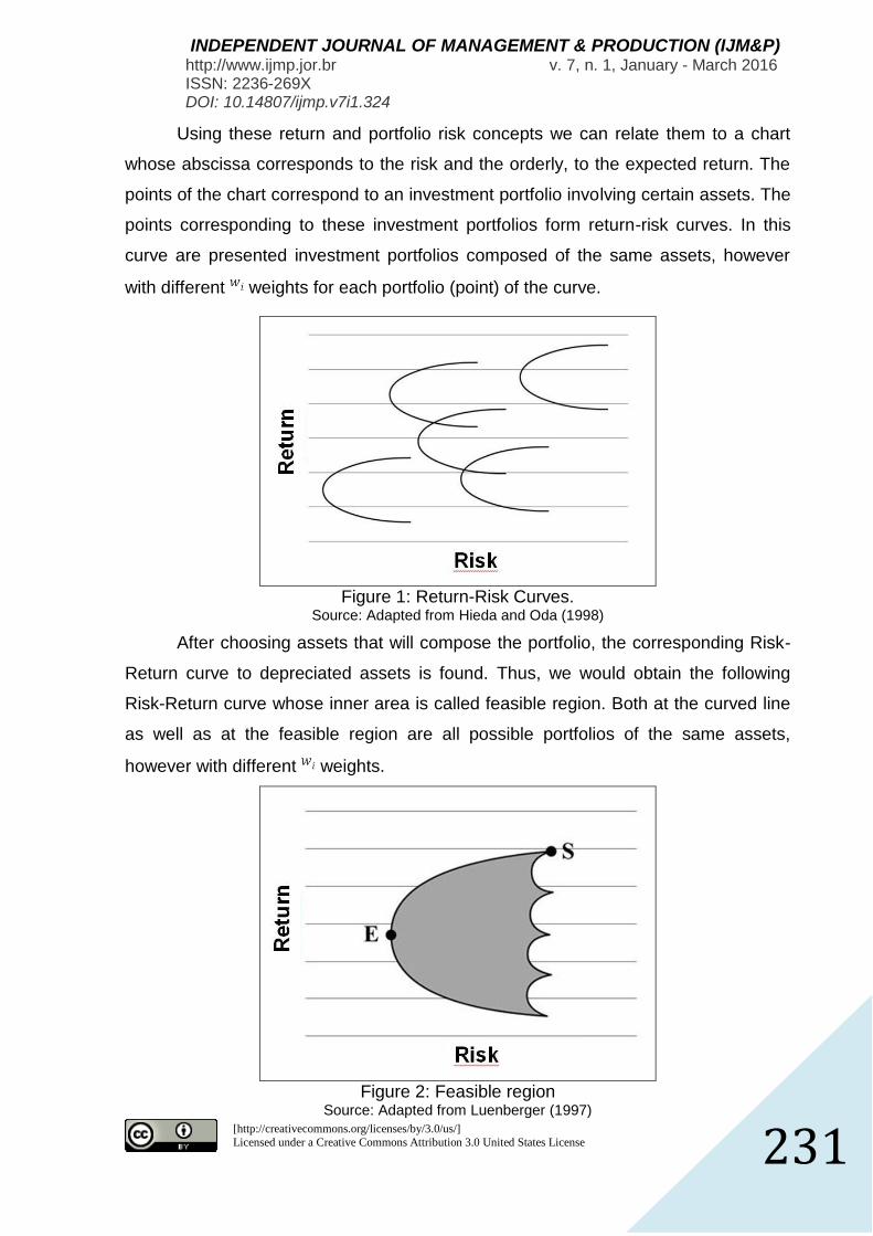
Using these return and portfolio risk concepts we can relate them to a chart

whose abscissa corresponds to the risk and the orderly, to the expected return. The

points of the chart correspond to an investment portfolio involving certain assets. The

points corresponding to these investment portfolios form return-risk curves. In this

curve are presented investment portfolios composed of the same assets, however

with different weights for each portfolio (point) of the curve.

Figure 1: Return-Risk Curves.

Source: Adapted from Hieda and Oda (1998)

After choosing assets that will compose the portfolio, the corresponding Risk-

Return curve to depreciated assets is found. Thus, we would obtain the following

Risk-Return curve whose inner area is called feasible region. Both at the curved line

as well as at the feasible region are all possible portfolios of the same assets,

however with different weights.

Figure 2: Feasible region

Source: Adapted from Luenberger (1997)




232

232

However the only part of the Risk-Return curve that follows the Dominance

principle, cited above, corresponds to the curved line that goes from point "E" of

minimal risk to point "S" of maximum return.

Figure 3: Efficient frontier

Source: Adapted from Hieda and Oda (1998)

The curve is called efficient frontier. Such boundary defines all the possible

efficient portfolio investments, that is, those that for a given level of return have the

minimum possible risk.

Finally, it is necessary to point out the relationship that the assets weights

have with their correlation index. Assuming a portfolio composed of two X and Y

assets, we form several X and Y combinations, each with a different correlation index

among the same and different weights. Thus, short selling is not possible (weight of

X + weight of Y = 1).

Chart 1: Correlation index

Source: Adapted from Bodie, Marcus and Kane (2010)




233

233

In it there is the following information on the assets correlation influence on the

diversification effects:

when the correlation between assets is positively perfect ( ), there is no

diversification effect of assets;

when the correlation between assets is imperfect , there are imperfect

effects of asset diversification;

when the correlation between assets is negatively perfect ( ), there is a

perfect effect of assets diversification shown by the scope of a risk equal to zero.

As the correlation between the two assets changes, the assets weights of the

portfolio must also be changed in order to maintain a certain level of risk. For

example, if it were necessary to maintain a minimum standard deviation, the asset X

should correspond to approximately 25%, 37.5% and 43.75% of the total portfolio, if

the correlations were, respectively, 0, 0.30 and -1 – assets of correlation perfect in

this case would not reach the aforementioned level of risk.

2.2. Investor preferences

Although the efficient frontier points the best investment combination

alternatives, there is nothing on which combination or which portfolio should be

selected, since this decision is up to each investor according to their personal

characteristics.

According to Danthine (2005), such preferences may take into account several

variables: the wealth degree of the investor, uncertainty in the investment time,

among others. However, a good instrument for assessing the preference of an

investor regarding the choice between risk assets is the indifference curve.




234

234

Figure 4: Risk aversion

Source: Adapted from Bodie, Marcus and Kane (2010)

The indifference curve measures the risk aversion degree of an investor, that

is, the amount of additional return they need to accept one more risk unit. In the

above, we observe three indifference curves. The steeper the curve, the greater the

risk aversion degree is. Thus, the curves "A", "B" and "C" correspond to investors of,

respectively, greater risk aversion, moderate risk aversion and lower risk aversion.

Similarly, risk aversion can also be calculated by the Sharpe index:

(7)

Where

= return of asset X;

= standard deviation of asset X.

It measures how much more return is given for each additional unit of risk.

3. METHODOLOGY

3.1. General data

The methodology involves the quantitative model analysis, exploring the

financial and statistical data from the top 10 companies of BM &, that is, companies

with relatively large amounts of shares traded. This information was drawn from the




235

235

company's Thomson Reuters Eikon database, a leader in collection and distribution

of information on the business market.

To carry out this work we considered the following periods as pre-crisis, crisis

and post-crisis scenarios.

Table 1: Analyzed periods Period Scenario

January/2004 to June/2007 Pre-crisis

July/2007 to June/2009 Crisis

July/2009 to December/2012 Post-crisis

Source: The author

The ten companies chosen for this study with their codes of their actions are

listed in Table 2.

Table 2 – Analyzed companies Action Code Company

BBAS3.SA Banco do Brasil

BBDC4.SA Banco Bradesco

CCRO3.SA Companhia de Concessões Rodoviárias

CMIG4.SA Companhia Energética de Minas Gerais,

CSNA3.SA Companhia Siderúrgica Nacional

EMBR3.SA Embraer

GGB Gerdau

ITUB.K Itaú Unibanco Holding

PETR4.SA Petrobrás

VALE5.SA Vale

Source: The author

3.2. Analysis of covariance

In order to identify the covariance behavior over time we structured

semiannual covariance matrices between the companies’ share returns. Each matrix

has the covariances of returns of the companies within a semester over eight years

(2004-2012). Furthermore, for matrices calculation we used the "COVARIAÇÃO.S"

tool from the Microsoft Excel program. The result of this formula is the deviation

average of products of each pair of points in two datasets, in this case, two sets

return of two different companies. Therefore, the matrix is composed of covariances

of all possible pairwise combinations of the ten aforementioned companies.

3.2.1. Constructing hypothetical portfolio

This section of the study primarily aims to quantify the influence of the

covariances instability in a theoretical portfolio, by changing the assets weights over

time.




236

236

First of all, we identified, for each of the three periods studied (pre-crisis, crisis

and post-crisis) their returns, standard deviations, and covariance matrices. From

these variables, we built six hypothetical portfolios. Three portfolios have restrictions

such as the preference of a Sharpe index of a hypothetical investor equal to 15% in

the three periods. The three other portfolios must maintain constant their weights, to

quantify the Sharpe index variation.

In order to find the returns, standard deviations and covariance matrices, we

used formulas showed in the theoretical foundation of this article. Whereas the

construction of portfolios that meet a Sharpe index of 15% were made by the

SOLVER tool from Microsoft Excel, under the following restrictions:

4. ANALYSIS OF COVARIANCE

The covariance matrices of the ten companies in the study are as follows.

Table 3: Covariance matrix of 1st semester of 2004

BBAS3 BBDC4 CCRO3 CMIG4 CSNA3 EMBR3 GGB ITUB.K PETR4 VALE5

BBAS3 0,13976 0,11425 0,00037 0,09142 0,15211 0,42324 0,04299 0,09565 0,16317 0,20200

BBDC4 0,11425 0,12120 0,00091- 0,09135 0,13951 0,40071 0,03578 0,09630 0,15204 0,21505

CCRO3 0,00037 0,00091- 0,01229 0,01088- 0,02338- 0,01371- 0,00772 0,00540- 0,01979- 0,02362-

CMIG4 0,09142 0,09135 0,01088- 0,10475 0,15355 0,36308 0,03320 0,08241 0,16759 0,15618

CSNA3 0,15211 0,13951 0,02338- 0,15355 0,37979 0,58122 0,06413 0,12466 0,28518 0,24623

EMBR3 0,42324 0,40071 0,01371- 0,36308 0,58122 1,71749 0,14847 0,34412 0,61310 0,68965

GGBR4 0,04299 0,03578 0,00772 0,03320 0,06413 0,14847 0,03546 0,03228 0,05752 0,03202

ITSA4 0,09565 0,09630 0,00540- 0,08241 0,12466 0,34412 0,03228 0,08837 0,14085 0,17904

PETR4 0,16317 0,15204 0,01979- 0,16759 0,28518 0,61310 0,05752 0,14085 0,31301 0,27015

VALE5 0,20200 0,21505 0,02362- 0,15618 0,24623 0,68965 0,03202 0,17904 0,27015 0,52373

1º SEMESTRE 2004

Source: The author

Table 4: Covariance matrix of 2nd semester 2004


BBAS3 0,64856 0,50188 0,28974 0,32087 0,20998 0,37874- 0,14621 0,41379 0,50461 0,80898

BBDC4 0,50188 0,42866 0,23101 0,25949 0,15590 0,27209- 0,10620 0,33990 0,39141 0,62594

CCRO3 0,28974 0,23101 0,14453 0,13471 0,11106 0,11970- 0,07363 0,19748 0,21035 0,37403

CMIG4 0,32087 0,25949 0,13471 0,20333 0,10143 0,26803- 0,08462 0,21442 0,30566 0,45203

CSNA3 0,20998 0,15590 0,11106 0,10143 0,14227 0,04589- 0,09791 0,14553 0,15100 0,31666

EMBR3 0,37874- 0,27209- 0,11970- 0,26803- 0,04589- 0,83688 0,10197- 0,23487- 0,52520- 0,58181-

GGBR4 0,14621 0,10620 0,07363 0,08462 0,09791 0,10197- 0,10318 0,11659 0,15830 0,27617

ITSA4 0,41379 0,33990 0,19748 0,21442 0,14553 0,23487- 0,11659 0,29874 0,35698 0,58470

PETR4 0,50461 0,39141 0,21035 0,30566 0,15100 0,52520- 0,15830 0,35698 0,57686 0,80603

VALE5 0,80898 0,62594 0,37403 0,45203 0,31666 0,58181- 0,27617 0,58470 0,80603 1,31350

2º SEMESTRE 2004

Source: The author




237

237



BBAS3 0,14786 0,00854- 0,00749 0,02390- 0,08254 0,14902 0,03161 0,00307 0,07713 0,11558

BBDC4 0,00854- 0,57346 0,00155- 0,19637 0,08807 0,14799 0,01299 0,27275 0,32895 0,10350

CCRO3 0,00749 0,00155- 0,01340 0,00338- 0,00165- 0,04050 0,01156 0,00508 0,02219 0,02741

CMIG4 0,02390- 0,19637 0,00338- 0,15862 0,17742- 0,09033- 0,08779- 0,11227 0,06689 0,20827-

CSNA3 0,08254 0,08807 0,00165- 0,17742- 1,07562 0,62375 0,32641 0,08363- 0,23824 1,10049

EMBR3 0,14902 0,14799 0,04050 0,09033- 0,62375 0,71186 0,23891 0,03237 0,33896 0,77870

GGBR4 0,03161 0,01299 0,01156 0,08779- 0,32641 0,23891 0,14799 0,01627- 0,07896 0,35271

ITSA4 0,00307 0,27275 0,00508 0,11227 0,08363- 0,03237 0,01627- 0,17005 0,15474 0,06616-

PETR4 0,07713 0,32895 0,02219 0,06689 0,23824 0,33896 0,07896 0,15474 0,38873 0,38035

VALE5 0,11558 0,10350 0,02741 0,20827- 1,10049 0,77870 0,35271 0,06616- 0,38035 1,34771

1º SEMESTRE 2005

Source: The author

Table 6: Covariance matrix of 2nd semester of 2005


BBAS3 0,99678 1,72126 0,23806 0,29896 0,21663 0,60271 0,62057 0,77516 1,07993 1,41330

BBDC4 1,72126 4,07016 0,59276 0,64877 0,36734 1,29271 1,25005 1,63812 2,17470 2,63051

CCRO3 0,23806 0,59276 0,10062 0,10011 0,05041 0,21639 0,19086 0,24514 0,32078 0,36927

CMIG4 0,29896 0,64877 0,10011 0,16006 0,13308 0,27138 0,23580 0,26584 0,47956 0,48064

CSNA3 0,21663 0,36734 0,05041 0,13308 0,18244 0,21190 0,18040 0,15971 0,42425 0,36817

EMBR3 0,60271 1,29271 0,21639 0,27138 0,21190 0,77816 0,50736 0,53947 0,91594 0,85563

GGBR4 0,62057 1,25005 0,19086 0,23580 0,18040 0,50736 0,48131 0,57144 0,81582 0,93038

ITSA4 0,77516 1,63812 0,24514 0,26584 0,15971 0,53947 0,57144 0,77098 0,93297 1,17970

PETR4 1,07993 2,17470 0,32078 0,47956 0,42425 0,91594 0,81582 0,93297 1,71862 1,70859

VALE5 1,41330 2,63051 0,36927 0,48064 0,36817 0,85563 0,93038 1,17970 1,70859 2,26387

2º SEMESTRE 2005

Source: The author



BBAS3 0,91431 0,74643 0,04024 0,13731 0,33277 0,13474 0,47867 0,53313 0,58171 0,37023

BBDC4 0,74643 2,36171 0,29970 0,65302 0,16667 0,74102 0,38252 0,88887 0,90018 0,80541

CCRO3 0,04024 0,29970 0,09673 0,11935 0,08782- 0,18634 0,07176- 0,01374 0,07494 0,15332

CMIG4 0,13731 0,65302 0,11935 0,28975 0,06071- 0,25450 0,07235- 0,10324 0,24364 0,34343

CSNA3 0,33277 0,16667 0,08782- 0,06071- 0,55456 0,14215- 0,51322 0,36640 0,43826 0,23457

EMBR3 0,13474 0,74102 0,18634 0,25450 0,14215- 0,82973 0,08886- 0,11435 0,21765 0,22611

GGBR4 0,47867 0,38252 0,07176- 0,07235- 0,51322 0,08886- 0,84355 0,74880 0,38300 0,12264

ITSA4 0,53313 0,88887 0,01374 0,10324 0,36640 0,11435 0,74880 0,99294 0,41380 0,16951

PETR4 0,58171 0,90018 0,07494 0,24364 0,43826 0,21765 0,38300 0,41380 0,88353 0,78227

VALE5 0,37023 0,80541 0,15332 0,34343 0,23457 0,22611 0,12264 0,16951 0,78227 1,04537

1º SEMESTRE 2006

Source: The author



BBAS3 1,37130 0,74643 0,69311 0,36081 0,06893- 0,91140 0,23478 0,66043 0,83426 1,94974

BBDC4 1,17289 1,31008 0,67595 0,29520 0,08279- 1,22776 0,14248 0,72975 0,53635 1,69341

CCRO3 0,69311 0,67595 0,41101 0,16231 0,08650- 0,66275 0,10133 0,40131 0,31675 0,93522

CMIG4 0,36081 0,29520 0,16231 0,13126 0,03092 0,15555 0,06943 0,15723 0,29658 0,60819

CSNA3 0,06893- 0,08279- 0,08650- 0,03092 0,12142 0,23705- 0,00244- 0,06338- 0,11092 0,06248

EMBR3 0,91140 1,22776 0,66275 0,15555 0,23705- 2,00436 0,06193- 0,73338 0,16400- 1,11316

GGBR4 0,23478 0,14248 0,10133 0,06943 0,00244- 0,06193- 0,17395 0,16058 0,30398 0,36304

ITSA4 0,66043 0,72975 0,40131 0,15723 0,06338- 0,73338 0,16058 0,60894 0,30288 0,99574

PETR4 0,83426 0,53635 0,31675 0,29658 0,11092 0,16400- 0,30398 0,30288 1,04439 1,42515

VALE5 1,94974 1,69341 0,93522 0,60819 0,06248 1,11316 0,36304 0,99574 1,42515 3,21538

2º SEMESTRE 2006

Source: The author



BBAS3 1,95447 1,55059 0,59248 0,73458 1,79245 0,36449 1,52807 1,44009 0,94343 2,95263

BBDC4 1,55059 1,71527 0,50276 0,55347 1,24199 0,03416- 1,04596 1,13766 0,91346 2,02145

CCRO3 0,59248 0,50276 0,23526 0,24036 0,59534 0,14763 0,50210 0,41877 0,34857 1,02566

CMIG4 0,73458 0,55347 0,24036 0,32861 0,68090 0,18940 0,63587 0,55590 0,44370 1,16171

CSNA3 1,79245 1,24199 0,59534 0,68090 2,41257 0,80712 1,59366 1,21309 0,73249 3,91059

EMBR3 0,36449 0,03416- 0,14763 0,18940 0,80712 0,68389 0,55657 0,26696 0,02220 1,50008

GGBR4 1,52807 1,04596 0,50210 0,63587 1,59366 0,55657 1,49018 1,23548 0,67336 2,64549

ITSA4 1,44009 1,13766 0,41877 0,55590 1,21309 0,26696 1,23548 1,29444 0,69618 1,95588

PETR4 0,94343 0,91346 0,34857 0,44370 0,73249 0,02220 0,67336 0,69618 1,04347 1,22648

VALE5 2,95263 2,02145 1,02566 1,16171 3,91059 1,50008 2,64549 1,95588 1,22648 6,97819

1º SEMESTRE 2007

Source: The author




238

238



BBAS3 1,10353 1,30060 0,03283 0,12836 1,16506 0,16569 0,32025 0,40727 2,23637 2,69811

BBDC4 1,30060 2,91733 0,33776- 0,07581- 2,98669 0,15428- 1,24517 1,63211 6,63272 7,34219

CCRO3 0,03283 0,33776- 0,28072 0,18061 0,60070- 0,20966 0,40561- 0,59232- 1,81161- 1,11298-

CMIG4 0,12836 0,07581- 0,18061 0,22560 0,35636- 0,23671 0,12199- 0,25331- 0,85223- 0,40863-

CSNA3 1,16506 2,98669 0,60070- 0,35636- 3,90496 0,50438- 1,12836 1,80241 8,40760 8,86823

EMBR3 0,16569 0,15428- 0,20966 0,23671 0,50438- 0,82725 0,23565- 0,24525- 1,36299- 1,31884-

GGBR4 0,32025 1,24517 0,40561- 0,12199- 1,12836 0,23565- 1,75059 2,02726 4,09370 2,75780

ITSA4 0,40727 1,63211 0,59232- 0,25331- 1,80241 0,24525- 2,02726 2,67194 5,57878 4,13921

PETR4 2,23637 6,63272 1,81161- 0,85223- 8,40760 1,36299- 4,09370 5,57878 23,11169 19,53912

VALE5 2,69811 7,34219 1,11298- 0,40863- 8,86823 1,31884- 2,75780 4,13921 19,53912 24,52083

2º SEMESTRE 2007

Source: The author



BBAS3 2,12778 0,82518 0,38739 0,57793 0,86635 0,28203- 0,97898 0,76947 2,72939 0,72102

BBDC4 0,82518 2,34019 0,52708 1,04348 4,20005 0,89839- 2,08556 0,32205 3,58118 3,63548

CCRO3 0,38739 0,52708 0,33101 0,46092 1,57699 0,84673- 1,61526 0,38926 1,47475 0,80937

CMIG4 0,57793 1,04348 0,46092 0,88828 2,63096 1,53501- 2,85297 0,81148 2,46916 1,48113

CSNA3 0,86635 4,20005 1,57699 2,63096 13,42529 4,47486- 7,75553 0,85962 9,58663 8,34521

EMBR3 0,28203- 0,89839- 0,84673- 1,53501- 4,47486- 4,26714 6,86607- 1,89321- 3,33189- 0,72964-

GGBR4 0,97898 2,08556 1,61526 2,85297 7,75553 6,86607- 12,76269 4,10880 6,71522 2,43176

ITSA4 0,76947 0,32205 0,38926 0,81148 0,85962 1,89321- 4,10880 2,36199 1,80052 0,00355

PETR4 2,72939 3,58118 1,47475 2,46916 9,58663 3,33189- 6,71522 1,80052 11,00839 6,69479

VALE5 0,72102 3,63548 0,80937 1,48113 8,34521 0,72964- 2,43176 0,00355 6,69479 8,21875

1º SEMESTRE 2008

Source: The author



BBAS3 7,72622 6,27814 1,88239 0,92553 13,64128 3,37084 18,27491 9,07395 15,15383 14,07742

BBDC4 6,27814 5,47312 1,56032 0,85640 11,15312 2,54475 14,60481 7,02226 12,34112 11,51012

CCRO3 1,88239 1,56032 0,57868 0,25522 3,48150 0,71373 4,35487 2,02395 3,54119 3,51304

CMIG4 0,92553 0,85640 0,25522 0,41635 1,73620 0,04110 2,18008 0,84860 1,92916 1,88641

CSNA3 13,64128 11,15312 3,48150 1,73620 26,20954 5,27812 34,50097 16,85438 28,25051 26,70725

EMBR3 3,37084 2,54475 0,71373 0,04110 5,27812 2,68585 7,62911 4,28697 5,87474 5,26867

GGBR4 18,27491 14,60481 4,35487 2,18008 34,50097 7,62911 50,75190 25,77196 38,51761 34,92815

ITSA4 9,07395 7,02226 2,02395 0,84860 16,85438 4,28697 25,77196 13,97273 19,20479 17,04780

PETR4 15,15383 12,34112 3,54119 1,92916 28,25051 5,87474 38,51761 19,20479 34,00734 29,82375

VALE5 14,07742 11,51012 3,51304 1,88641 26,70725 5,26867 34,92815 17,04780 29,82375 28,23413

2º SEMESTRE 2008

Source: The author



BBAS3 4,97446 4,72829 1,23288 0,70893 4,64459 0,52488 0,68810 1,87534 6,15330 3,69955

BBDC4 4,72829 4,80855 1,26065 0,65862 4,63667 0,78386 0,69970 1,90940 5,88143 3,88590

CCRO3 1,23288 1,26065 0,41390 0,15382 1,27835 0,24503 0,40182 0,75307 1,41097 1,04435

CMIG4 0,70893 0,65862 0,15382 0,14061 0,62646 0,05766 0,06232 0,21036 0,87905 0,46476

CSNA3 4,64459 4,63667 1,27835 0,62646 5,00449 0,88044 0,97980 2,23040 5,84075 4,22374

EMBR3 0,52488 0,78386 0,24503 0,05766 0,88044 1,05649 0,16319- 0,42860 0,23845 0,80982

GGBR4 0,68810 0,69970 0,40182 0,06232 0,97980 0,16319- 1,38387 1,34977 0,79628 0,80861

ITSA4 1,87534 1,90940 0,75307 0,21036 2,23040 0,42860 1,34977 2,06206 1,89831 1,68284

PETR4 6,15330 5,88143 1,41097 0,87905 5,84075 0,23845 0,79628 1,89831 8,71967 5,09480

VALE5 3,69955 3,88590 1,04435 0,46476 4,22374 0,80982 0,80861 1,68284 5,09480 4,32041

1º SEMESTRE 2009

Source: The author



BBAS3 6,48752 5,23065 1,34217 0,96436 5,47145 0,70238 4,18699 5,05748 5,54585 9,15269

BBDC4 5,23065 4,77715 1,39568 1,02959 4,67192 0,29974 4,01282 4,67541 4,97745 8,29724

CCRO3 1,34217 1,39568 0,58866 0,40730 1,28176 0,13812- 1,61047 1,73529 1,60896 2,69423

CMIG4 0,96436 1,02959 0,40730 0,37875 0,93061 0,01728- 1,12373 1,16467 1,16014 1,87067

CSNA3 5,47145 4,67192 1,28176 0,93061 5,27897 0,45883 3,71879 4,49624 5,17922 8,66868

EMBR3 0,70238 0,29974 0,13812- 0,01728- 0,45883 0,62430 0,29452- 0,10478- 0,07070 0,18411

GGBR4 4,18699 4,01282 1,61047 1,12373 3,71879 0,29452- 5,31814 5,56190 4,86126 7,95266

ITSA4 5,05748 4,67541 1,73529 1,16467 4,49624 0,10478- 5,56190 6,24557 5,37819 9,15391

PETR4 5,54585 4,97745 1,60896 1,16014 5,17922 0,07070 4,86126 5,37819 5,90644 9,45604

VALE5 9,15269 8,29724 2,69423 1,87067 8,66868 0,18411 7,95266 9,15391 9,45604 15,97958

2º SEMESTRE 2009

Source: The author




239

239



BBAS3 1,08944 0,73256 0,19359 0,00155 1,73424 0,17111 0,46600- 0,21039- 2,12857 2,34394

BBDC4 0,73256 0,85974 0,25670 0,04373 1,03349 0,07978 0,14926- 0,11200 2,01804 1,77293

CCRO3 0,19359 0,25670 0,14372 0,02394 0,27534 0,02265 0,05263- 0,06537 0,73855 0,55989

CMIG4 0,00155 0,04373 0,02394 0,07343 0,03003- 0,00449 0,02209 0,04939 0,00338- 0,03164-

CSNA3 1,73424 1,03349 0,27534 0,03003- 5,09103 0,57168 1,97714- 1,37557- 3,17656 5,58419

EMBR3 0,17111 0,07978 0,02265 0,00449 0,57168 0,09328 0,21785- 0,15104- 0,25836 0,58616

GGBR4 0,46600- 0,14926- 0,05263- 0,02209 1,97714- 0,21785- 1,80335 1,41815 0,87970- 1,68629-

ITSA4 0,21039- 0,11200 0,06537 0,04939 1,37557- 0,15104- 1,41815 1,31919 0,18726- 0,92683-

PETR4 2,12857 2,01804 0,73855 0,00338- 3,17656 0,25836 0,87970- 0,18726- 6,97530 4,96873

VALE5 2,34394 1,77293 0,55989 0,03164- 5,58419 0,58616 1,68629- 0,92683- 4,96873 7,34228

1º SEMESTRE 2010

Source: The author



BBAS3 3,40240 3,42213 1,39321 0,70688 0,32427 1,17502 0,00087 2,49599 0,80192- 5,41290

BBDC4 3,42213 3,66904 1,43975 0,74256 0,46996 1,31222 0,21248 2,59831 0,68891- 5,59098

CCRO3 1,39321 1,43975 0,73127 0,36650 0,01583- 0,58101 0,01583- 1,46768 0,42569- 2,59975

CMIG4 0,70688 0,74256 0,36650 0,25356 0,04109- 0,29455 0,02508 0,81171 0,26463- 1,34494

CSNA3 0,32427 0,46996 0,01583- 0,04109- 0,67079 0,14690 0,21385 0,53972- 0,43702 0,15393

EMBR3 1,17502 1,31222 0,58101 0,29455 0,14690 0,71667 0,09043 1,51817 0,21939- 2,51005

GGBR4 0,00087 0,21248 0,01583- 0,02508 0,21385 0,09043 0,51314 0,09650- 0,17555 0,32831-

ITSA4 2,49599 2,59831 1,46768 0,81171 0,53972- 1,51817 0,09650- 4,96337 1,15739- 6,28677

PETR4 0,80192- 0,68891- 0,42569- 0,26463- 0,43702 0,21939- 0,17555 1,15739- 0,97604 1,54011-

VALE5 5,41290 5,59098 2,59975 1,34494 0,15393 2,51005 0,32831- 6,28677 1,54011- 11,47598

2º SEMESTRE 2010

Source: The author



BBAS3 0,79822 0,59042 0,04161- 0,36680- 1,46740 0,11869 0,25946 0,16578 0,78162 1,67941

BBDC4 0,59042 0,65341 0,00337 0,05542- 0,79986 0,01671- 0,15687 0,01190 0,59703 0,88418

CCRO3 0,04161- 0,00337 0,08936 0,17132 0,19877- 0,04529- 0,04623- 0,04959- 0,15646- 0,32945-

CMIG4 0,36680- 0,05542- 0,17132 0,70559 1,37979- 0,28497- 0,45119- 0,17199- 0,85557- 1,58893-

CSNA3 1,46740 0,79986 0,19877- 1,37979- 4,59986 0,75149 1,26877 0,06779 2,76336 4,44762

EMBR3 0,11869 0,01671- 0,04529- 0,28497- 0,75149 0,38654 0,43554 0,09248- 0,63768 0,58966

GGBR4 0,25946 0,15687 0,04623- 0,45119- 1,26877 0,43554 1,00068 0,11815- 1,21954 0,95741

ITSA4 0,16578 0,01190 0,04959- 0,17199- 0,06779 0,09248- 0,11815- 0,76527 0,31299- 0,49460

PETR4 0,78162 0,59703 0,15646- 0,85557- 2,76336 0,63768 1,21954 0,31299- 2,52832 2,47082

VALE5 1,67941 0,88418 0,32945- 1,58893- 4,44762 0,58966 0,95741 0,49460 2,47082 5,55003

1º SEMESTRE 2011

Source: The author



BBAS3 0,94184 0,32735 0,01359 0,06451 0,79585 0,01943 0,49539 0,83722 0,43950 1,24707

BBDC4 0,32735 1,84759 0,25530 0,73496 0,68553 0,77422 0,29217- 0,91346- 1,23619 1,11320

CCRO3 0,01359 0,25530 0,19628 0,04502 0,07708- 0,19559 0,26257- 0,61149- 0,09010- 0,15141-

CMIG4 0,06451 0,73496 0,04502 0,66208 0,30233 0,13216 0,09352 0,13238 0,83090 0,39456

CSNA3 0,79585 0,68553 0,07708- 0,30233 1,22668 0,31416 0,49297 0,68831 0,98532 2,03871

EMBR3 0,01943 0,77422 0,19559 0,13216 0,31416 0,78836 0,47663- 1,19702- 0,26121 0,74284

GGBR4 0,49539 0,29217- 0,26257- 0,09352 0,49297 0,47663- 1,30919 2,48687 0,34631 0,61319

ITSA4 0,83722 0,91346- 0,61149- 0,13238 0,68831 1,19702- 2,48687 5,25696 0,52274 0,69582

PETR4 0,43950 1,23619 0,09010- 0,83090 0,98532 0,26121 0,34631 0,52274 1,88634 1,84458

VALE5 1,24707 1,11320 0,15141- 0,39456 2,03871 0,74284 0,61319 0,69582 1,84458 4,26115

2º SEMESTRE 2011

Source: The author



BBAS3 6,67060 2,04988 1,84880- 3,13166- 4,06216 1,14158- 0,66529- 2,02945 5,13989 3,17027

BBDC4 2,04988 1,18492 0,71320- 1,18599- 1,23358 0,66608- 0,29070- 0,18684 1,77561 1,08012

CCRO3 1,84880- 0,71320- 1,87426 2,91973 1,26993- 1,40975 1,07824 0,40327 2,03368- 0,75057-

CMIG4 3,13166- 1,18599- 2,91973 4,99766 1,95533- 2,59944 1,81474 0,91131 3,37632- 0,97113-

CSNA3 4,06216 1,23358 1,26993- 1,95533- 2,84367 0,38658- 0,31901- 1,70771 3,30038 2,18217

EMBR3 1,14158- 0,66608- 1,40975 2,59944 0,38658- 1,97924 1,27085 1,54689 1,41576- 0,13378-

GGBR4 0,66529- 0,29070- 1,07824 1,81474 0,31901- 1,27085 1,13765 1,22575 0,96669- 0,38715-

ITSA4 2,02945 0,18684 0,40327 0,91131 1,70771 1,54689 1,22575 3,18869 1,03238 1,01533

PETR4 5,13989 1,77561 2,03368- 3,37632- 3,30038 1,41576- 0,96669- 1,03238 4,51638 2,64995

VALE5 3,17027 1,08012 0,75057- 0,97113- 2,18217 0,13378- 0,38715- 1,01533 2,64995 3,18750

1º SEMESTRE 2012

Source: The author




240

240



BBAS3 3,28933 2,17496 0,58054 2,36866- 0,74883 0,47601 0,34863 0,51171 1,68187 0,32253-

BBDC4 2,17496 2,80084 0,87850 2,20863- 0,47513 0,41649 0,30763 0,03131- 0,40935 0,67816

CCRO3 0,58054 0,87850 0,77622 1,93930- 0,00769- 0,28620 0,39916 0,37758 0,01264 0,24862

CMIG4 2,36866- 2,20863- 1,93930- 12,71010 0,94578- 1,41416- 2,00817- 2,86852- 1,24497- 1,50049-

CSNA3 0,74883 0,47513 0,00769- 0,94578- 0,55198 0,18891 0,08100 0,23511 0,54562 0,67921

EMBR3 0,47601 0,41649 0,28620 1,41416- 0,18891 0,36323 0,23326 0,35360 0,30879 0,12144

GGBR4 0,34863 0,30763 0,39916 2,00817- 0,08100 0,23326 0,47938 0,63210 0,23014 0,02634-

ITSA4 0,51171 0,03131- 0,37758 2,86852- 0,23511 0,35360 0,63210 1,10605 0,65776 0,07442-

PETR4 1,68187 0,40935 0,01264 1,24497- 0,54562 0,30879 0,23014 0,65776 1,80913 0,81695-

VALE5 0,32253- 0,67816 0,24862 1,50049- 0,67921 0,12144 0,02634- 0,07442- 0,81695- 3,92926

2º SEMESTRE 2012

Source: The author

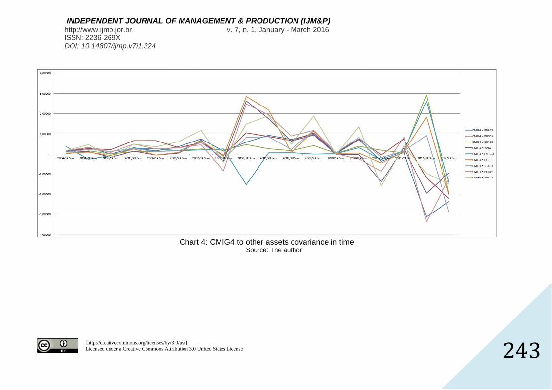
Based on these matrices (Table 3 to 20), we can infer that the covariances are

not stable over time, which would put at risk the maintenance over time of portfolios

of investment according to the Markowitz model (1952). It is also important to note

that these variabilities further increase in periods of crisis, when a significant increase

in covariance is observed among the majority of shares in 2007 and, especially, in

2008.

There is a reasonable peak increase in the 2nd semester of 2007, followed by

a slight drop in the 1st semester of 2008. And later, a substantially higher peak –

approximately, 700% higher – in the 1st semester of 2008, reaching the maximum

covariance of the nine years studied in this work. Thus, in general, the tables present

a growing instability in the 1st semester of 2004 until the 2nd semester of 2007, when

the summit is reached in 2008. Consecutively, from the 1st semester of 2009 until the

2nd semester of 2012, instabilities are perceived and they still exist, although

decreasing.

Another secondary result is the stable relation of CMIG4 and CCRO3 have

when compared to the others. Using a simple measurement of dispersion, namely

the interval of variation, calculated by the difference between the maximum and

minimum in the observation dataset, we found that CMIG4 and CCRO4 had 6,29%

and 6,38% of variation respectively. As opposed to the GGB share with a very

unstable variation of 45,38%.

In the following chart such a conclusion can be more visually observed.




241

Chart 2: Behavior of covariance between shares returns over time

Source: The author




242

Chart 3: CCRO2 to other assets covariance in time

Source: The author




243

Chart 4: CMIG4 to other assets covariance in time

Source: The author




244

Chart 5: GGB to other assets covariance in time

Source: The author

5. CONSTRUCTING HYPOTHETICAL PORTFOLIO

After concluding that the instability of the covariances between the shares not only exist, but it is also significant, a more

particular evaluation of these oscillations is necessary, from the construction of six hypothetical portfolios in relation to the periods of

pre-crisis, crisis and post-crisis. These portfolios seek to identify the influence of covariance instability in the maintenance cost of

the portfolios.

[http://creativecommons.org/licenses/by/3.0/us/] Licensed under a Creative Commons Attribution 3.0 United States License


245

We formed two species of hypothetical portfolios for each period

aforementioned. Both types of portfolios do not allow short selling, that is,

. However, one of them has as a constraint, obtaining a Sharpe index

equivalent to 15% for its formation. The other portfolio genre should present constant

asset weight over time, and it starts with a distribution that generates a Sharpe index

also equivalent to 15%. In the following we present the data to obtain each portfolio –

returns, standard deviations and covariance matrices – as well as the construction of

portfolios with the respective weights of each asset.

5.1. Hypothetical portfolio pre-crisis: January/2004 to June/2007

Table 21: Data for individual assets in the pre-crisis period

Assets μ σ

BBAS3 253,20% 365,21%

BBDC4 270,12% 499,17%

CCRO3 416,51% 143,23%

CMIG4 129,92% 152,94%

CSNA3 150,99% 179,99%

EMBR3 20,23% 282,37%

GGBR4 410,43% 248,11%

ITUB.K 352,20% 339,76%

PETR4 160,81% 422,94%

VALE5 187,09% 538,25%

Source: The author

Table 22: Covariance between assets in the pre-crisis period

BBAS3 BBDC4 CCRO3 CMIG4 CSNA3 EMBR3 GGBR4 ITUB.K PETR4 VALE5

BBAS3 13.34 17.44 5.03 5.26 5.82 8.82 8.77 12.02 14.54 18.95

BBDC4 17.44 24.92 6.73 7.41 7.29 11.78 11.63 16.65 20.62 24.60

CCRO3 5.03 6.73 2.05 2.03 2.20 3.36 3.32 4.67 5.53 7.39

CMIG4 5.26 7.41 2.03 2.34 2.18 3.32 3.47 4.99 6.21 7.50

CSNA3 5.82 7.29 2.20 2.18 3.24 4.14 4.06 5.18 6.21 8.73

EMBR3 8.82 11.78 3.36 3.32 4.14 7.97 6.03 8.02 9.94 12.44

GGBR4 8.77 11.63 3.32 3.47 4.06 6.03 6.16 8.12 9.91 12.35

ITUB.K 12.02 16.65 4.67 4.99 5.18 8.02 8.12 11.54 13.86 17.15

PETR4 14.54 20.62 5.53 6.21 6.21 9.94 9.91 13.86 17.89 20.21

VALE5 18.95 24.60 7.39 7.50 8.73 12.44 12.35 17.15 20.21 28.97

Source: The author



246

246

Table 23: Assets portfolios in the pre-crisis period

IS = 15% Constant weights

Assets Wi

BBAS3 0,00% 0,00%

BBDC4 0,00% 0,00%

CCRO3 0,00% 0,00%

CMIG4 0,00% 0,00%

CSNA3 0,00% 0,00%

EMBR3 83,83% 83,83%

GGBR4 0,00% 0,00%

ITUB.K 0,00% 0,00%

PETR4 4,14% 4,14%

VALE5 12,03% 12,03%

Σwi 100,00% 100,00%

μp 46,12% 46,12%

σp 307,46% 307,46%

IS 15,00% 15,00%

Source: The author

5.2. Crisis hypothetical portfolio: July/2007 to June/2009

Table 24: Data for individual assets in the pre-crisis period Assets μ σ

BBAS3 20,72% 387,24%

BBDC4 25,78% 311,41%

CCRO3 22,57% 101,15%

CMIG4 5,70% 74,18%

CSNA3 86,07% 498,03%

EMBR3 -56,67% 432,06%

GGBR4 35,35% 511,16%

ITUB.K 33,09% 344,08%

PETR4 51,00% 570,36%

VALE5 22,14% 701,37%

Source: The author



247

247

Table 25: Covariance between assets in the pre-crisis period BBAS3 BBDC4 CCRO3 CMIG4 CSNA3 EMBR3 GGBR4 ITUB.K PETR4 VALE5

BBAS3 15,00 11,22 3,19 1,06 12,46 7,31 10,07 10,40 14,87 20,75

BBDC4 11,22 9,70 2,32 0,87 11,38 6,17 9,52 8,65 13,50 18,82

CCRO3 3,19 2,32 1,02 0,48 2,40 0,61 1,89 2,04 2,35 3,33

CMIG4 1,06 0,87 0,48 0,55 0,89 -0,76 1,11 0,72 0,71 0,41

CSNA3 12,46 11,38 2,40 0,89 24,80 1,15 16,62 11,14 26,07 24,47

EMBR3 7,31 6,17 0,61 -0,76 1,15 18,67 7,11 6,63 4,01 19,90

GGBR4 10,07 9,52 1,89 1,11 16,62 7,11 26,13 15,20 18,12 21,90

ITUB.K 10,40 8,65 2,04 0,72 11,14 6,63 15,20 11,84 13,22 18,07

PETR4 14,87 13,50 2,35 0,71 26,07 4,01 18,12 13,22 32,53 31,19

VALE5 20,75 18,82 3,33 0,41 24,47 19,90 21,90 18,07 31,19 49,19 Source: The author

Table 26: Assets portfolios in the crisis period IS = 15% Constant weights

Assets Wi

BBAS3 0,00% 0,00%

BBDC4 3,46% 0,00%

CCRO3 20,09% 0,00%

CMIG4 14,89% 0,00%

CSNA3 28,16% 0,00%

EMBR3 0,00% 83,83%

GGBR4 9,22% 0,00%

ITUB.K 13,46% 0,00%

PETR4 10,72% 4,14%

VALE5 0,00% 12,03%

Σwi 100,00% 100,00%

μp 43,69% -42,73%

σp 291,27% 429,97%

IS 15,00% -9,94%

Source: The author

5.3. Hypothetical portfolio post-crisis: July/2009 to December/2012

Table 27: Data for individual assets in the post-crisis period Assets μ σ

BBAS3 -4,74% 214,79%

BBDC4 -24,48% 225,07%

CCRO3 -118,61% 296,50%

CMIG4 -47,94% 358,54%

CSNA3 50,82% 527,22%

EMBR3 -56,65% 174,90%

GGBR4 47,29% 289,20%

ITUB.K 31,06% 285,78%

PETR4 42,40% 360,04%

VALE5 -8,45% 300,85%

Source: The author



248

248

Table 28: Covariance between assets in the post-crisis period BBAS3 BBDC4 CCRO3 CMIG4 CSNA3 EMBR3 GGBR4 ITUB.K PETR4 VALE5

BBAS3 4,61 1,23 -2,49 -3,74 7,24 -0,54 2,65 3,65 3,70 4,23

BBDC4 1,23 5,07 4,64 3,48 -4,36 2,61 -2,67 -2,06 -2,73 0,82

CCRO3 -2,49 4,64 8,79 8,23 -12,63 4,07 -5,79 -5,54 -6,77 -2,95

CMIG4 -3,74 3,48 8,23 12,86 -13,52 4,38 -6,81 -5,61 -7,55 -3,43

CSNA3 7,24 -4,36 -12,63 -13,52 27,80 -4,83 13,09 10,35 15,87 8,90

EMBR3 -0,54 2,61 4,07 4,38 -4,83 3,06 -2,58 -1,42 -3,26 0,25

GGBR4 2,65 -2,67 -5,79 -6,81 13,09 -2,58 8,36 5,61 8,19 2,69

ITUB.K 3,65 -2,06 -5,54 -5,61 10,35 -1,42 5,61 8,17 4,75 5,10

PETR4 3,70 -2,73 -6,77 -7,55 15,87 -3,26 8,19 4,75 12,96 4,16

VALE5 4,23 0,82 -2,95 -3,43 8,90 0,25 2,69 5,10 4,16 9,05 Source: The author

Table 29: Assets portfolios in the post-crisis period

IS = 15% Constant weights

Assets Wi

BBAS3 0.00% 0.00%

BBDC4 0.00% 0.00%

CCRO3 0.00% 0.00%

CMIG4 0.00% 0.00%

CSNA3 0.34% 0.00%

EMBR3 0.00% 83.83%

GGBR4 39.48% 0.00%

ITUB.K 29.28% 0.00%

PETR4 30.90% 4.14%

VALE5 0.00% 12.03%

Σwi 100.00% 100.00%

μp 41.04% -46.75%

σp 273.60% 147.23%

IS 15.00% -31.75%

Source: The author

Where:

= return of a given asset in the corresponding period;

= standard deviation of a given asset in the corresponding period;

SI = Sharpe index;

Σwi = total sum of assets weights;

= total expected return of the portfolio;

= total standard deviation of a portfolio.



249

249

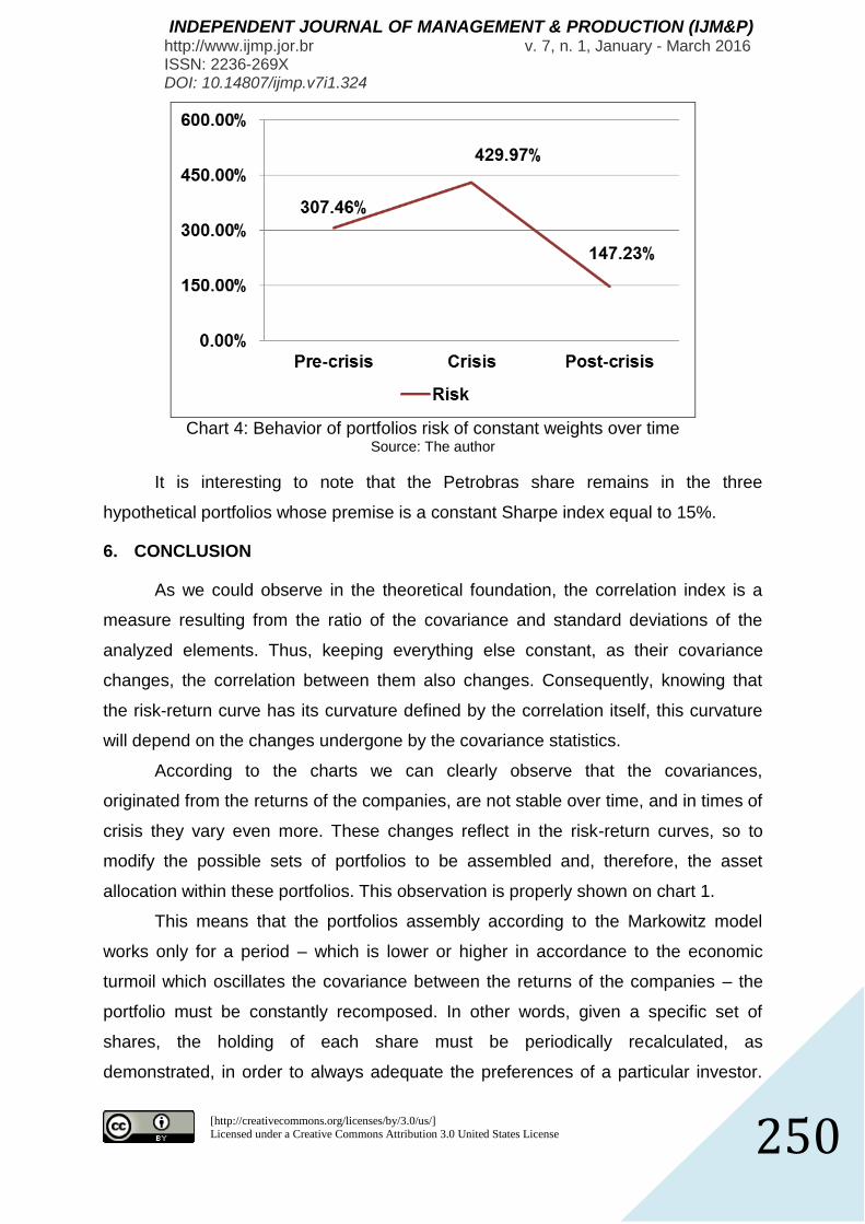
The preferences of return and risk of an investor are one of the most important

factors to be considered in assembling portfolios, as seen in the theory. From this

analysis it is evident that in order to maintain such preferences, in the case of a rate

of beyond 15% of return for each additional unit of risk, it is necessary to change

periodically the assets weights in the hypothetical portfolio. If the investor does not

recalculate the assets weights of their portfolio as shown by the type of hypothetical

portfolio of constant weights, their preference regarding return and risk expected is

not met over time. Nevertheless, if the investor wishes to rescue the application in

times of crisis or post-crisis, they will have a loss of -42.73% or -46.75%,

respectively, of the initial investment made in January 2004 (pre-crisis). The behavior

of returns and risks during the studied period can be verified according to the

following charts.

Charts 3: Behavior of portfolio returns of constant weights over time Source: The author



250

250

Chart 4: Behavior of portfolios risk of constant weights over time

Source: The author

It is interesting to note that the Petrobras share remains in the three

hypothetical portfolios whose premise is a constant Sharpe index equal to 15%.

6. CONCLUSION

As we could observe in the theoretical foundation, the correlation index is a

measure resulting from the ratio of the covariance and standard deviations of the

analyzed elements. Thus, keeping everything else constant, as their covariance

changes, the correlation between them also changes. Consequently, knowing that

the risk-return curve has its curvature defined by the correlation itself, this curvature

will depend on the changes undergone by the covariance statistics.

According to the charts we can clearly observe that the covariances,

originated from the returns of the companies, are not stable over time, and in times of

crisis they vary even more. These changes reflect in the risk-return curves, so to

modify the possible sets of portfolios to be assembled and, therefore, the asset

allocation within these portfolios. This observation is properly shown on chart 1.

This means that the portfolios assembly according to the Markowitz model

works only for a period – which is lower or higher in accordance to the economic

turmoil which oscillates the covariance between the returns of the companies – the

portfolio must be constantly recomposed. In other words, given a specific set of

shares, the holding of each share must be periodically recalculated, as

demonstrated, in order to always adequate the preferences of a particular investor.



251

251

As demonstrated in this research, share weights will change more in the portfolio in

times of crisis, in which the covariances between companies change substantially.

Periodically recalculate the holding of each asset of the investment portfolio is

a possible solution to the instability problem of covariance over time. However, it

might increase the maintenance costs of portfolio which will be as costly as larger are

the covariance volatilities. Another interesting solution to be explored in future studies

is by identifying portfolios according to the degree of stability of their covariances

which could be measured most precisely with the aid of a statistical hypothesis test.

REFERENCES

ALMEIDA, N.; SILVA, R. F.; RIBEIRO, K.(2010) Aplicação do modelo de Markowitz na seleção de carteiras eficientes: uma análise de cenários no mercado de capitais brasileiro. XIII Seminários em administração, Uberlândia. Setembro.

HIEDA, A.; ODA, A. L. (1998) Um estudo sobre a utilização de dados históricos no modelo de Markowitz aplicado a Bolsa de Valores de São Paulo. In: Seminários de Administração, 3, Out. 1998, São Paulo. Anais do III SEMEAD. São Paulo: Faculdade de Economia, Administração e Contabilidade da USP.

BODIE, Z.; MARCUS, A. J.; KANE, A. (2010) Investimentos. New York: Artmed.

DANTHINE, J.; DONALDSON, J. B. (2005) Intermediate financial theory. California: Elsevier.

LUENBERGER, D. G. (1997) Investment Science. USA: Oxford University Press. p. 137-172.

MARKOWITZ, Harry M. (1952) Portfólio selection. Journal of Finance, v. 7, n. 1, p. 77-91. Mar.

PENTEADO, M. A.; FAMÁ, R. (2002) Será que o beta que temos é o beta que queremos?. Cadernos de pesquisas em administração, São Paulo, v. 09, n. 3, julho/setembro.

SHARPE, William F.; ALEXANDER, GORDON J.; BAILEY, JEFFERY V. (1995) Investments. NewJersey: Prentice Hall.

Documents

MODELO PARA A FORMATAÇÃO DOS ARTIGOS A SEREM … · Licensed under a Creative Commons Attribution 3.0 United States License [ INDEPENDENT JOURNAL OF MANAGEMENT