Modelling wave–current interactions off the east coast … A. D. Sabatino et al.: Modelling wave–current interactions off the east coast of Scotland study carried out byTolman(1991)

Ocean Sci., 12, 875–897, 2016www.ocean-sci.net/12/875/2016/doi:10.5194/os-12-875-2016© Author(s) 2016. CC Attribution 3.0 License.

Modelling wave–current interactions off the east coast of ScotlandAlessandro D. Sabatino1, Chris McCaig1,a, Rory B. O’Hara Murray2, and Michael R. Heath1

1Marine Population Modelling Group, Department of Mathematics and Statistics,University of Strathclyde, Glasgow, UK2Marine Scotland Science, Marine Laboratory, Aberdeen, UKanow at: Brookes Bell, 280 St. Vincent Street, Glasgow, UK

Correspondence to: Alessandro D. Sabatino ([email protected])

Received: 20 November 2015 – Published in Ocean Sci. Discuss.: 18 December 2015Revised: 14 April 2016 – Accepted: 15 April 2016 – Published: 5 July 2016

Abstract. Densely populated coastal areas of the North Seaare particularly vulnerable to severe wave conditions, whichovertop or damage sea defences leading to dangerous flood-ing. Around the shallow southern North Sea, where thecoastal margin is lying low and population density is high,oceanographic modelling has helped to develop forecastingsystems to predict flood risk. However, coastal areas of thedeeper northern North Sea are also subject to regular stormdamage, but there has been little or no effort to developcoastal wave models for these waters. Here, we present a highspatial resolution model of northeast Scottish coastal waters,simulating waves and the effect of tidal currents on wavepropagation, driven by global ocean tides, far-field wave con-ditions, and local air pressure and wind stress. We show thatthe wave–current interactions and wave–wave interactionsare particularly important for simulating the wave conditionsclose to the coast at various locations. The model can simu-late the extreme conditions experienced when high (spring)tides are combined with sea-level surges and large Atlanticswell. Such a combination of extremes represents a high riskfor damaging conditions along the Scottish coast.

1 Introduction

Due to its semi-enclosed morphology and shoalingbathymetry, the North Sea experiences extreme wave condi-tions, in particular during winter periods (Woolf et al., 2002).When combined with sea-level surges such events can leadto damaging inundation of low-lying coastal regions, due to

wave overtopping of sea defences. Development of a mod-elling and predictive capability for high-resolution wave con-ditions in the North Sea is therefore a high priority. How-ever, the task is complicated due to interaction between lo-cally generated waves and incoming swell from outside theregion, and especially due to interactions between waves andtidal currents.

Crossing, or bimodal, sea states occur between 5 and 40 %of the time in the North Sea (Guedes Soares, 1984). Theseare generated when swell waves propagating into the re-gion from distant storm events interact with locally generatedwaves which may be of very different direction, period, andheight. Swell waves from the North Atlantic and the Norwe-gian Sea propagate into the North Sea, interacting with localwind-sea-generated waves, modifying the main spectral pa-rameters. The interaction between differing wave trains is notfully understood, but crossing seas have been statistically as-sociated with freak wave incidence, and shipping accidents(Waseda et al., 2011; Tamura et al., 2009; Cavaleri et al.,2012; Onorato et al., 2006, 2010; Sabatino and Serio, 2015;Toffoli et al., 2011a). The North Sea is particularly proneto rogue wave events, such as the famous Draupner waverecorded in 1994 (Haver, 2004), the first ever recorded roguewave event, that occurred in crossing sea conditions (Adcocket al., 2011). In the paper, the effect of the enhancement ofthe wind-sea waves due to swell is assessed during storms.

In addition to crossing seas, wave–current interactions area well-known cause of wave height amplification or atten-uation. Wave–current interactions (WCIs) are depth- andcurrent-induced modification of wave features. A seminal

Published by Copernicus Publications on behalf of the European Geosciences Union.

876 A. D. Sabatino et al.: Modelling wave–current interactions off the east coast of Scotland

study carried out by Tolman (1991) highlighted that WCIsare significant in the North Sea, changing the significantwave height (Hs) and the mean wave period (Tm) by 5 and10 %, respectively, during storm periods. However, the modelthat was used by Tolman (1991) to assess this effect was atvery course resolution and broad scale. In particular, the ef-fect of the WCI in the coastal shallow areas was not con-sidered. Phillips (1977) showed that in the absence of wavebreaking, local wave amplitude is given by

A

A0=

c0√c(c+ 2U)

, (1)

where A is the resulting wave amplitude, A0 is the unper-turbed amplitude of the wave field, c is the wave phase speed,and U is the current that interacts with the wave train. It isimportant to notice that the sign of the current is determinanton the effect of the WCI: if the current travels in opposite di-rection with the wave train, there will be an enhancement ofthe significant wave height. Conversely, if current and wavesare in the same direction, the Hs decreases. For deep waterwaves, the phase speed c depends only on the period of thewave, while in shallow water c depends only on the depth.Equation (1) shows that the waves travelling in a directionopposing the current (U < 0) have a positive ratio A/A0 andconsequently, an enhancement of the wave amplitude.

WCIs could also lead to the breaking of the wave: if thecurrent is strong enough to block the wave train (Ris andHolthuijsen, 1996), these waves can break and lose energybefore arriving to the coastline (Chawla and Kirby, 2002,1998).

WCIs are particularly difficult to quantify empirically, andcomputationally intensive to model. In addition, the WCIsare a well-known mechanism for the formation of roguewaves in the ocean: the Agulhas current, that flows near thecoastline of South Africa, was one of the first places in whichthis mechanism was identified (Mallory, 1974; Lavrenov,1998; Lavrenov and Porubov, 2006). Recently, many studies(Onorato et al., 2011; Toffoli et al., 2013, 2015; Shrira andSlunyaev, 2014; Ma et al., 2013) highlighted that the interac-tion between a train of waves with an adverse current couldincrease its wave steepness, and cause rogue waves due to themodulational instability (Benjamin and Feir, 1967). How-ever, it is clear that shallow coastal waters, embayments, andheadlands are particular foci for interactions (Hearn et al.,1987; Signell et al., 1990a). Model studies have concentratedon comparing wave height and period in coupled and uncou-pled model versions showing, for example, 3 % difference inwave height and 20 % in wave period in the Dutch and Ger-man coastal waters of the North Sea (Osuna and Monbaliu,2004). Similar results have been obtained for coastal wa-ters of the Adriatic during bora conditions (Benetazzo et al.,2013), finding a maximum reduction for the Hs of 0.6 m inthe central Adriatic and a simultaneous increase up to 0.5 min the gulfs of Trieste and Venice. WCIs were also studied

during hurricane conditions off the eastern seaboard of theUSA (Xie et al., 2008).

Sea defences of coastal settlements along the northeastcoast of Scotland have suffered several damaging events dur-ing the period 2009–2014 as a result of surges and waves.The coastal waters are dominated by strong tidal currentsand wind-driven residuals, are exposed to wave trains enter-ing the North Sea from the north, and generated by stormevents in the central and southern North Sea. Although theoceanography of the North Sea as a whole has been inten-sively studied since the 1830s (Whewell, 1830; Proudmanand Doodson, 1924; Dietrich, 1950; Huthnance, 1991; Ottoet al., 1990), and the region was one of the earliest to be sub-jected to computational hydrodynamic modelling (Flather,1987; Davies et al., 1985), high-resolution modelling activityhas been largely concentrated in areas with potential for waveand tidal energy extraction (Adcock et al., 2013; Bryden andCouch, 2006; Baston and Harris, 2011; Shields et al., 2011,2009). However, there are no such models for the northeastcoast of mainland Scotland, and none which include coupledWCIs. Our objective here was to develop and test such amodel for the stretch of coastline between the Firth of Tayand Peterhead, centred on the strategically important portcity of Aberdeen and the town of Stonehaven (Fig. 1). Thelatter is the base for a governmentally supported marine mon-itoring site with a > 15-year time series of high-resolutiondata on a wide range of environmental parameters (Bresnanet al., 2009).

2 Materials and methods

The MIKE by DHI model was used to simulate the tidal-and wind-driven circulation, and the wave propagation. TheMIKE software is composed of different modules, for thecreation of a model grid and input files and to simulate differ-ent hydrodynamical features at the same time or separately.The following modules were used:

– The MIKE Zero modules for generating the computa-tional grid and the input files.

– The MIKE 3 FM module for simulating the tidal and thewind-driven circulation.

– The MIKE 21 SW module for modelling the wave prop-agation.

For the simulation of the WCIs, a one-way coupling be-tween MIKE 3 FM and MIKE 21 SW was set up. The depthaverage flow fields and the water level output from MIKE 3FM was provided as input to the MIKE 21 SW model.

2.1 The computational grid

Both MIKE 3 FM and MIKE 21 SW use an unstructuredgrid approach, with triangular elements (Ferziger and Peric,

Ocean Sci., 12, 875–897, 2016 www.ocean-sci.net/12/875/2016/

A. D. Sabatino et al.: Modelling wave–current interactions off the east coast of Scotland 877

Figure 1. The area studied in the present paper.

Figure 2. The computational grid generated with MIKE Zero soft-ware.

2002). Unstructured grids can represent complex coastlinesbetter than a rectangular grid and potentially provide morerealistic flows, enabling the geography of the coastline toaffect the propagation of tidal and surface waves in a re-alistic manner. In addition, triangular grid elements allow

smoothly changing cell sizes across a region, with the highestresolution concentrated in an area of particular interest. Themesh for the area of study is shown in Fig. 2. An enhanced-resolution area was created near Stonehaven, because thiswork is part of a wider study focusing on the resuspension ofthe sediments in this part of the domain. This high-resolutionarea also covered the Firth of Forth and the Aberdeenshirecoastline, where previous studies have shown enhanced cur-rents due to interaction between the tidal wave and the Scot-tish coastline (Dietrich, 1950; Otto et al., 1990).

2.2 The MIKE 3 FM hydrodynamic model

MIKE 3 FM (flow model) is based on the numerical solutionof the 3-D incompressible Reynolds-averaged Navier–Stokesequations, under the Boussinesq and the hydrostatic pres-sure approximations (DHI, 2011a). The spatial discretizationof the primitive equations is performed using a cell-centredfinite-volume method. In the finite-volume method the vol-ume integrals in the partial differential equations with a di-vergence are converted to surface integrals using the Gauss–Ostrogradsky theorem (Toro, 2009).

MIKE 3 FM has a flexible approach for simulating theflow in the water column. It is possible to choose betweensigma layers (Song and Haidvogel, 1994), z layers, andcoupled sigma and z layers. For our purpose we decidedto use the equidistant sigma layers approach, because thebathymetry of the area was not sufficiently complex to re-quire a more accurate description with a coupled sigma andz layer that would be extremely computationally expensive.Sigma layers are also useful for resolving the water columnwell throughout the tidal cycle, given the large tidal range.

www.ocean-sci.net/12/875/2016/ Ocean Sci., 12, 875–897, 2016


The coupled sigma and z layers were tested, but there was nosignificant improvement for simulating the flow.

For the horizontal eddy viscosity the formulation proposedby Smagorinsky (1963) was used, in which the sub-grid-scale transport is expressed by an effective eddy viscosityrelated to a characteristic length scale rather than a constanteddy viscosity. This sub-grid-scale viscosity is given by

A= c2s l

2√2SijSij , (2)

where cs is the Smagorinsky constant, l is the characteristiclength of the grid size, and the deformation rate is given by(Lilly, 1966; Deardorff, 1971; Smagorinsky, 1963)

Sij =12

(∂ui

∂xj+∂uj

∂xi

). (3)

The bed resistance was parameterized using a constantquadratic drag coefficient cf . The average bottom stress isdetermined by a quadratic friction law:

τb = cf ρ0ub |ub| , (4)

where ub is the average flow velocity above the bottom andρ0 is the density of the water. The value of the above param-eters chosen for the model are reported in Sect. 3.1.

The model was forced with a time series of tidal elevationsat the open boundaries from the open-source OSU (OregonState University) Tidal Prediction Software (OTPS) (Egbertet al., 2010), based on TOPEX satellite observation of thewater-level observations interpolated with tide gauge datafrom the European shelf region. In order to take account ofthe wind-driven circulation and surge in the model, meteoro-logical forcing was applied across the model domain, usingthe ERA-Interim reanalysis for wind velocity and mean sea-level pressure (Dee et al., 2011).

2.3 The MIKE 21 SW wave model

The MIKE 21 SW (spectral wave) is an unstructured gridmodel for wave prediction and analysis (DHI, 2011b). TheMIKE 21 SW is based on the wave action conservation equa-tion (Komen et al., 1996; Young, 1999), where the dependentvariable is the frequency-directional wave action spectrum.This is given by

∂N

∂t+∇ · (cN)=

S

σ, (5)

where S is the energy source term, defined as

S = Sin+ Snl+ Sds+ Sbot+ Ssurf (6)

that depends on the energy transfer from the wind to the wavefield Sin, on the nonlinear wave–wave interaction Snl, on thedissipation due to depth-induced wave breaking Ssurf, on thedissipation due to bottom friction Sbot, and on the dissipationcaused by the white-capping Sds.

The wave action density spectrum N(σ ,θ ) is defined as(Bretherton and Garrett, 1968)

N(σ,θ)=E(σ,θ)

σ, (7)

where E is the wave energy density spectrum, σ = 2πf isthe angular frequency (where f is the frequency), and θ is thedirection of wave propagation. The momentum transfer fromthe wind to the waves follows the formulation in Komen et al.(1996). The momentum transfer and the drag depend not onlyon the strength of the wind but also on the wave state itself.

For the physics of the propagation and breaking of thewaves we choose the following parameters:

– The depth-induced wave breaking is based on the for-mulation of Battjes and Janssen (1978), in which thegamma parameter is a constant 0.6 across the domain.The formulation of the depth-induced wave breakingcan be written as

Ssurf(σ,θ)=−αQbσH

2m

8πE(σ,θ)

Etot, (8)

where α ≈ 1.0 is a calibration constant, Qb is the frac-tion of breaking waves, σ is the spectrum average fre-quency, Etot is the total wave energy that is linked to thewave action density spectrum, and Hm is the estimatedmaximum wave height, that is defined as Hm = γ d

(Battjes and Janssen, 1978), in which d is the depth andγ is the free breaking parameter (Battjes, 1974).

– The bottom friction is specified in the model as theNikuradze roughness (kN) (Nikuradse, 1933; Johnsonand Kofoed-Hansen, 2000).

– The white-capping formulation described in Komenet al. (1996) in order to consider the dissipation ofwaves, based on the theory of Hasselmann (1974). Forthe fully spectral formulation, the white capping as-sumes a form that is dependent on the mean frequencyσ and on the wavenumber k:

Sds(σ,θ)=−Cds

(k2m0

)2

[(1− δ)

k

k+ δ

(k

k

)2]σN(σ,θ). (9)

Here the two parameters, Cds and δ, are the two dissipa-tion coefficients that control the overall dissipation rateand the strength of dissipation in the energy/action spec-trum, respectively, and m0 is the zeroth moment of theoverall spectrum.

The values of the above parameters chosen for the modelare reported in Sect. 3.2.



The model also included nonlinear energy transfer suchas the quadruplet wave interaction (Komen et al., 1996) andthe triad wave interaction which is the dominant nonlinearinteraction in shallow water (Eldeberky and Battjes, 1995,1996).

The forcings included in the model are the local windand the swell wave field from outside the model area andspecified at the model boundaries. For the model bound-aries we used boundary conditions from the Venugopal andNemalidinne (2014, 2015) North Atlantic model, a largerwave model that encompass the southern Norwegian Sea andthe North Atlantic Ocean. The ERA-Interim 0.125◦×0.125◦

model was used to provide a wind field across the model do-main with a time resolution of 6 h (Dee et al., 2011; Berris-ford et al., 2011).

2.4 Wave–current interactions

The WCIs are implemented using a one-way coupling be-tween currents and waves. The model was run without andwith currents implemented, and then the differences betweenthe two runs were studied. The WCIs in the MIKE modelare taken in account in the dispersion relation for the angularfrequency term, since the current due by tides and wind af-fect the propagation and changes the wavelength of the wavetrain. The MIKE 21 SW dispersion relation in fact is

σ =√gk tanh(kd)= ω− k ·U. (10)

The one-way coupling has, however, some limitationssince it is not taking into account the modification of the cur-rent by the wave itself (Michaud et al., 2011; Bennis et al.,2011).

2.5 Swell detection

In the present study, the wind-sea and the swell waves andtheir interaction are studied. MIKE 21 SW gives the oppor-tunity to separate spectrally the windsea waves and the swellwaves. There are two criteria, based on a dynamic threshold,available to make this separation.

The first criterion is based on the difference of the energybetween the spectrum and the fully developed sea condition(Earle, 1984). In this case, the threshold frequency is identi-fied as

fthreshold = αfp,PM

(EPM

EModel

)β, (11)

where α = 0.7, β = 0.31, EModel is the total energy at eachnode point calculated by the MIKE 21 SW model, and thePierson–Moskowitz peak frequency and the energy are esti-mated as

fPM = 0.14g

U10(12)

EPM =

(U10

1.4g

)4

. (13)

The second method is based on the wave-age criterion(Drennan et al., 2003) from empirical wave measurementsin wave tanks and in Lake Ontario field measurements. FromDonelan et al. (1985), swell waves are the components ful-filling the following relation:

U10

cpcos(θ − θw) < 0.83, (14)

where U10 is the wind speed at 10 m, cp is the phase speed,θ is the wave propagation direction, and θw is the directionof the wind. For discriminate swell and windsea waves weused the second method, since it is the most widely used forthis purpose and is the more reliable method (Drennan et al.,2003).

2.6 Validation data sets

The model was validated using five independent data sets.The hydrodynamic model was validated using data from theUK National Tide Gauge Network in Aberdeen and Leithand using the tide gauge data from the Scottish Environ-mental Protection Agency (SEPA) in Buckie. Validation wasperformed comparing harmonic components extracted fromtime series of both model and real data. The harmonic com-ponents of the sea level were extracted using the UTide Mat-lab function (Codiga, 2011).

Current meter observations from the British Oceano-graphic Data Centre (BODC) were used to validate the mod-elled currents. For the wave model, we compared recordeddata from wave gauges in the Moray Firth and in the Firthof Forth (obtained from CEFAS) and data from a wave riderbuoy deployed in Aberdeen Bay (data obtained from Uni-versity of Aberdeen). In addition, we used significant waveheight and mean wave period from satellite data provided byWaveNet (CEFAS) for June 2008. Especially important inthis case is the Aberdeen wave gauge, since this is the onlyone in shallow water (the depth of the sea in the mooring lo-cation is 10 m). This allows us to evaluate the ability of themodel in coastal areas, in which the WCIs are strongest.

Table 1 shows details of the observations used for validat-ing and calibrating the tidal and wave model, while in Fig. S1in the Supplement we show the position of the tide and wavegauges used for the validation and the position of the satellitedata.

The validation for waves was carried out using four statis-tical indices: the bias, the root mean square error (RMSE),the correlation coefficient (R), and the scatter index (SI).These indices are defined below.

Bias=1N

N∑i=1

(xoi − xmi

)(15)

RMSE=

√√√√ 1N

N∑i=1

(xoi − xmi

)2 (16)



Table 1. Location of the validation/calibration instrumentation.

Description Coordinates Depth (m) Use

longitude (◦) latitude (◦)Aberdeen tide gauge −2.0803 57.144 – water level val/calLeith tide gauge −3.1682 55.9898 – water level validationBuckie tide gauge −2.9667 57.6667 – water level validationFirth of Forth buoy −2.5038 56.1882 – waves validationMoray Firth buoy −3.3331 57.9663 – waves val/calAberdeen wave rider −2.0500 57.1608 – waves validationBODC 4551 RCM −2.8000 57.7910 12 current validationBODC 4561 RCM −1.9680 57.2320 12 current validationBODC 4562 RCM −1.9680 57.2320 27 current validationBODC 4571 RCM −1.9020 57.2260 12 current validationBODC 4572 RCM −1.9020 57.2260 52 current validationBODC 4582 RCM −2.1500 56.9870 23 current validationBODC 4591 RCM −2.0980 56.9820 12 current validationBODC 4592 RCM −2.0980 56.9820 47 current validation

R =

N∑i=1

(xoi − xo

)(xmi − xm

)√

N∑i=1

(xoi − xo

)2(xmi − xm

)2 (17)

SI=RMSExo

(18)

For tidal current validation we used, instead of the SI, thenormalized root mean square error (NRMSE), that is definedas

NRMSE=RMSE

max(x)−min(x). (19)

The validation was performed for different years. For thehydrodynamic model the agreement between modelled andobserved water level was evaluated for the entire year 2007,while the currents were validated for 1992, where the rotorcurrent meter observations were available. The wave modelwas validated for 2010 and 2008, where observations andboundary inputs were available.

3 Results

3.1 Calibration and validation of the hydrodynamicmodel

The hydrodynamic model was calibrated for the year 2007,based on the agreement with the recorded water level at thetide gauge in Aberdeen. The calibration parameters werethe time step that was fixed at 1 s after an analysis ofthe Courant–Friedrichs–Lewy (CFL) conditions (higher timesteps were investigated but the model was unstable); theSmagorinsky constant that was set to 0.2 (for values > 0.3the model showed some blow-up); and the bottom rough-ness that was parameterized with the drag coefficient cf =

Table 2. Computed RMSE for the main harmonic components, thevalidation for each tide gauge is reported in the Table S1.

Components RMSE

A (cm) g (◦)M2 2.52 0.78S2 1.64 3.68N2 1.31 3.02O1 0.76 5.42K1 0.44 14.4Q1 0.42 13.6

0.0025. After calibration, the MIKE 3 tidal model was vali-dated against harmonic components extracted from both ob-served and modelled data for water level. The agreement be-tween modelled and observed currents was also investigated.RMSE for the amplitude of harmonic components was lessthan 1 % for all the cases, while the phase of the main semid-iurnal component was well modelled. In particular for thedominant M2 component, the phase error was very low andthe amplitude was well modelled (see Tables 2 and S1 in theSupplement for more details). The validation results showthat the modelled results are in good agreement with therecorded tidal amplitude and phase. The model was run for1992 and measurements obtained from BODC from eight lo-cations were used to validate the currents in the model. Thevalidation of the single components u and v is reported inTable S2. Table 3 shows that the model adequately repre-sents the current speeds in the domain. The validation showsthat the model slightly underestimates the current, howeverit can be noticed that the bias of the model was very low. TheRMSE, except for one observation, does not exceed 15 % ofthe maximum speed.



Table 3. Results from the validation of the currents, showing the difference between the modelled and observed current speeds at the eightlocations reported in Table 1.

RCM no. Lat Long Depth RMSE NRMSE R2 Bias(m) (m s−1) (m s−1)

4551 −2.8 57.791 12 0.094 0.157 0.17 0.0014561 −1.968 57.232 12 0.111 0.124 0.70 −0.034562 −1.968 57.232 27 0.075 0.105 0.75 −0.024571 −1.902 57.226 12 0.223 0.147 0.23 −0.054572 −1.902 57.226 52 0.087 0.112 0.80 −0.024582 −2.15 56.987 23 0.075 0.124 0.80 0.024591 −2.098 56.982 12 0.125 0.132 0.73 −0.0624592 −2.098 56.982 47 0.073 0.121 0.82 −0.05

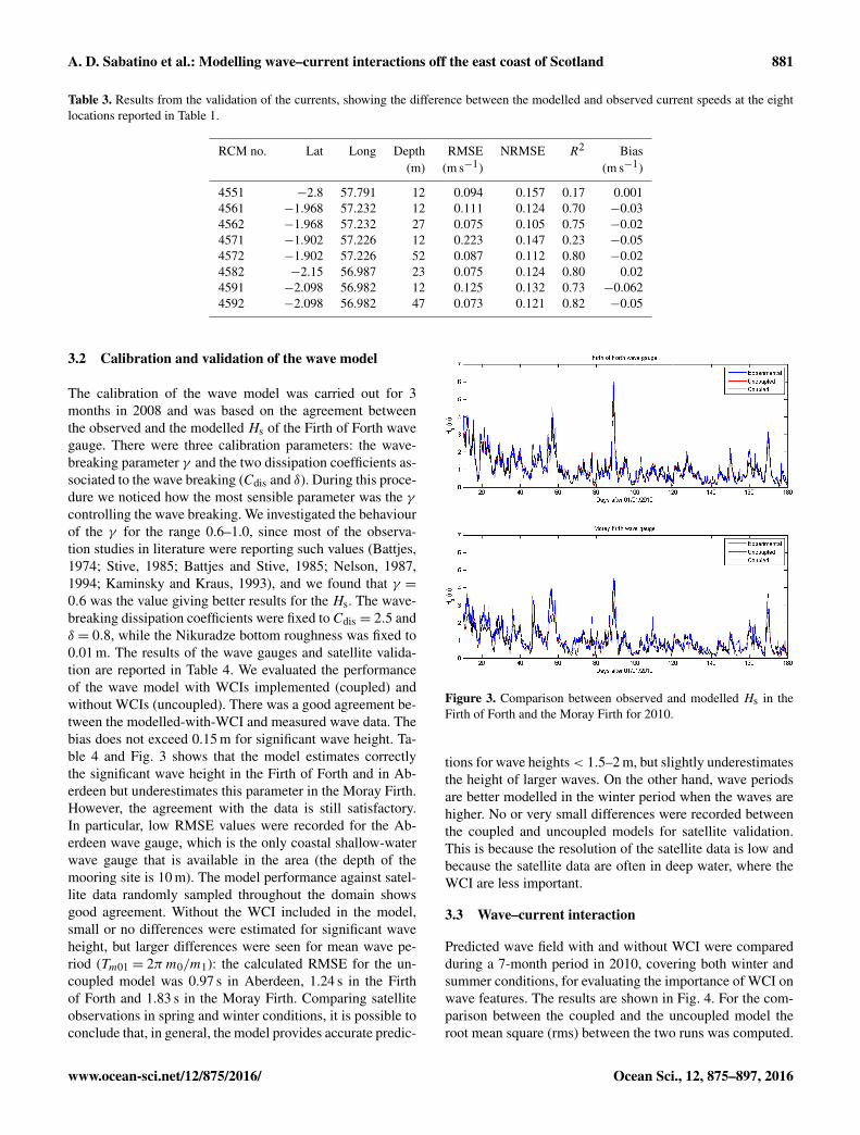
3.2 Calibration and validation of the wave model

The calibration of the wave model was carried out for 3months in 2008 and was based on the agreement betweenthe observed and the modelled Hs of the Firth of Forth wavegauge. There were three calibration parameters: the wave-breaking parameter γ and the two dissipation coefficients as-sociated to the wave breaking (Cdis and δ). During this proce-dure we noticed how the most sensible parameter was the γcontrolling the wave breaking. We investigated the behaviourof the γ for the range 0.6–1.0, since most of the observa-tion studies in literature were reporting such values (Battjes,1974; Stive, 1985; Battjes and Stive, 1985; Nelson, 1987,1994; Kaminsky and Kraus, 1993), and we found that γ =0.6 was the value giving better results for the Hs. The wave-breaking dissipation coefficients were fixed to Cdis = 2.5 andδ = 0.8, while the Nikuradze bottom roughness was fixed to0.01 m. The results of the wave gauges and satellite valida-tion are reported in Table 4. We evaluated the performanceof the wave model with WCIs implemented (coupled) andwithout WCIs (uncoupled). There was a good agreement be-tween the modelled-with-WCI and measured wave data. Thebias does not exceed 0.15 m for significant wave height. Ta-ble 4 and Fig. 3 shows that the model estimates correctlythe significant wave height in the Firth of Forth and in Ab-erdeen but underestimates this parameter in the Moray Firth.However, the agreement with the data is still satisfactory.In particular, low RMSE values were recorded for the Ab-erdeen wave gauge, which is the only coastal shallow-waterwave gauge that is available in the area (the depth of themooring site is 10 m). The model performance against satel-lite data randomly sampled throughout the domain showsgood agreement. Without the WCI included in the model,small or no differences were estimated for significant waveheight, but larger differences were seen for mean wave pe-riod (Tm01 = 2π m0/m1): the calculated RMSE for the un-coupled model was 0.97 s in Aberdeen, 1.24 s in the Firthof Forth and 1.83 s in the Moray Firth. Comparing satelliteobservations in spring and winter conditions, it is possible toconclude that, in general, the model provides accurate predic-

Figure 3. Comparison between observed and modelled Hs in theFirth of Forth and the Moray Firth for 2010.

tions for wave heights< 1.5–2 m, but slightly underestimatesthe height of larger waves. On the other hand, wave periodsare better modelled in the winter period when the waves arehigher. No or very small differences were recorded betweenthe coupled and uncoupled models for satellite validation.This is because the resolution of the satellite data is low andbecause the satellite data are often in deep water, where theWCI are less important.

3.3 Wave–current interaction

Predicted wave field with and without WCI were comparedduring a 7-month period in 2010, covering both winter andsummer conditions, for evaluating the importance of WCI onwave features. The results are shown in Fig. 4. For the com-parison between the coupled and the uncoupled model theroot mean square (rms) between the two runs was computed.



Table 4. Comparison between observed and modelled (both with and without WCIs implemented) wave heights and periods for wave gaugesand satellite observations. The reported validation was carried out for 2010 (Firth of Forth and Moray Firth) and for 2008 (Aberdeen wavegauge and satellite observations). Details of the observation data are reported in Table 1 of the paper and in Table S2 of the Supplement.

Coupled Uncoupled

Bias RMSE R SI Bias RMSE R SIFirth of ForthHs −0.02 m 0.30 m 0.941 0.27 −0.01 m 0.30 m 0.939 0.27Tm −0.70 s 1.17 s 0.767 0.25 −0.76 s 1.24 s 0.758 0.27Moray FirthHs −0.14 m 0.42 m 0.849 0.38 −0.15 m 0.42 m 0.848 0.39Tm −1.18 s 1.75 s 0.668 0.39 −1.23 s 1.83 s 0.656 0.41AberdeenHs −0.07 m 0.21 m 0.836 0.32 −0.07 m 0.22 m 0.831 0.32Tm −0.25 s 0.91 s 0.715 0.20 −0.30 s 0.97 s 0.701 0.21SatelliteWinterHs −0.2 m 0.4 m – 0.25 −0.2 m 0.4 m – 0.25Tm +0 s 0.8 s – 0.15 +0 s 0.8 s – 0.15SpringHs −0.1 m 0.3 m – 0.21 −0.1 m 0.3 m – 0.21Tm +0.1 s 1.2 s – 0.23 +0.1 s 1.2 s – 0.23

Figure 4. Root mean square difference between wave model output with and without WCI: (a) significant wave height (m), (b) peak waveperiod (s), (c) wave directional spreading (degrees).

Results show some differences between the two runs. In par-ticular, the largest deviations due to WCI are found in coastalareas, such as around headlands and bays, and in estuaries, inwhich the currents (mostly driven by tides) are strongest. Asexpected, the highest differences were seen in the proximityof the coastline (Signell et al., 1990b): this was because thestrength of the mainly tidal-driven currents are stronger (Di-etrich, 1950; Otto et al., 1990). During spring tides, highervalues for the current were recorded off northeast Englandand near Peterhead and Aberdeen (see Fig. 1). Wave periodsare more affected than wave heights in this coupling, withrms deviations that can be on average 20 % (absolute value)in shallow-water coastal areas. We also considered the effectof the WCIs on the wave directional spreading, as this is animportant variable for the stability of the wave train in deepwater and for its evolution (Benjamin and Feir, 1967). The

results showed that during the 7-month period the significantwave height was, on average, less affected than directionalspreading or wave periods: the difference was of the orderof magnitude of 0.1 m near the coastline and less offshore,while the difference in peak spectral wave period (Tp) ex-ceeded 1 s in some of the east coast firths such as the MorayFirth and the Firth of Forth.

Maximum positive and negative variation during the 7-month period were also studied (Figs. 5 and 6). The figureis similar to the RMSE: the larger variation is reported onlyin the coastal areas, while in the open sea the maximum vari-ation is limited up to 1 m. Spatially, the maximum variationof Hs between the coupled and the uncoupled run was +2.8and−1.8 m, both occurring during storm events and both oc-curring in coastal areas, near the coast of Aberdeen and Pe-



Figure 5. Maximum modelled positive deviation of the Hs (m) dueto the WCIs recorded in the 7-month period run in 2010.

terhead and south of the Firth of Forth, in which the tidallydriven current is stronger (Dietrich, 1950; Otto et al., 1990).

3.4 Current and swell effect on the windsea wave field

In order to study the importance of the WCIs and the cou-pling between swell and windsea waves off the east coastof Scotland, three storms were considered in the periodJanuary–August 2010. Storm events were identified by ex-amining the time series in the Firth of Forth and the MorayFirth in which the highest Hs were recorded. These threestorms were selected because they were the three most in-tense storms during the considered period and originatedfrom different weather conditions.

3.4.1 The 26–27 February 2010 storm

Between 25 and 27 February 2010, the UK was affected bya low pressure system, that moved rapidly from west to east.From the afternoon of the 25th to the 26th, the centre of thestorm was over the North Sea (Fig. 7). At the same time,another low pressure system (not shown in the map) wasover the Norwegian Sea, causing a train of swell movingfrom north to south. Comparison of modelled and observa-tion wave heights and wave period conditions for this stormare reported in Fig. 8. In addition, the modelled conditionsin the Aberdeen wave rider location are reported. The figureshows that the model reproduces adequately the conditionsduring that storm, in particular around the time in which themaximum Hs was reached.

The low pressure over North Sea caused windsea wavesexceeding 4 m. In Fig. 9 the situation in the sea is shown at

Figure 6. Maximum modelled negative deviation of theHs (m) dueto the WCIs recorded in the 7-month period run in 2010.

12:30 UTC of the 26th: swell waves contributed to enhancingtheHs in the centre of the storm, while a train of swell waveswas forming from this storm, travelling west to the MorayFirth. Interaction of the windsea and the swell waves causedhigh waves along the east coast: the maximum recorded Hsby the Firth of Forth wave gauge was 4.8 m. WCI contributedto the enhancement ofHs by up to 1 m in coastal areas, whilein the open sea the contribution was very low, up to 0.1 m. Inthe afternoon of the 26th (Fig. 10, at 19:00 UTC) the stormwas near the Firth of Forth. The contribution of the swellwaves was significant, increasing theHs by up to 1 m: modeloutputs showed that the central part of the storm had anHs >

5 m, while without the swell coming from north the centre ofthe storm would have been anHs< 4.5 m. To our knowledge,no significant damages were recorded for this storm.

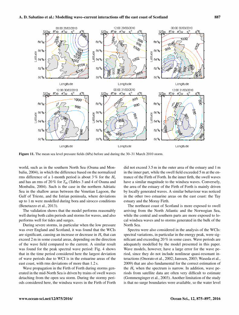
3.4.2 The 30–31 March 2010 storm

The larger storm in 2010 occurred during the night of30 March 2010. Between 29 March and 1 April 2010 thesoutheast coast of Scotland and the north of England werestruck by severe weather and very strong winds. These con-ditions were caused by a strong depression that originatedfrom a weak minimum near the Azores islands, in the NorthAtlantic, in front of the Portuguese coast. This low pressurewas < 990 hPa once over Great Britain and Ireland at mid-night of 30 March 2010 and reached its minimum the day af-ter with a depression of< 980 hPa over the north of England.The evolution of the storm from surface pressure charts fromECMWF ERA-Interim reanalysis is reported in Fig. 11 (Deeet al., 2011; Berrisford et al., 2011). These figures clearlyshow that the depression, at its maximum strength, is just



Figure 7. The mean sea level pressure fields (hPa) before and during the 25–26 March 2010 storm.

above the south of Scotland during the night between 30 and31 March 2010. This depression generated both very highwaves (Hs exceeded 6 m, measured in the Firth of Forth)and surge waves exceeding 0.5 m (measured both by the Ab-erdeen and Leith tide gauges). The waves caused signifi-cant damages to the coastal defences of cities in the south-east of Scotland. In particular, the City of Edinburgh Coun-cil estimated the damages to coastal defences to be aboutGBP 23 000. Also, in Berwick, at the southern entrance ofthe Firth of Forth, some damages were caused to the har-bour infrastructures. To the east, in Dumbar, waves toppedthe roofs of two-floor houses.

Damaging conditions associated with this storm werecaused by a combination of simultaneous factors: (1) tidesin the spring period, (2) a surge wave of about 0.5 m gener-ated by local pressure and wind, (3) windsea waves generatedlocally that interacted with strong currents, (4) a weak butsignificant swell waves field that interacted with the windseawaves.

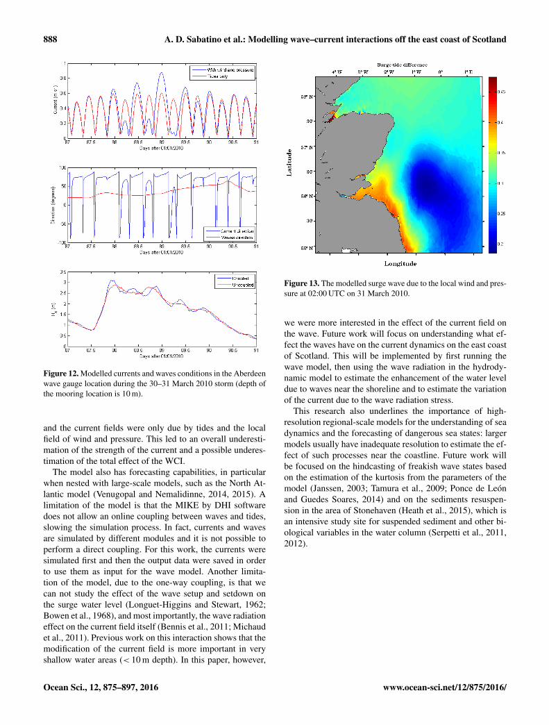
Figure 12 shows the intensity of the current in the Ab-erdeen wave gauge location and the resulting WCI. It can beseen that the current was strongly enhanced by the wind, andconsequently the WCI effect was stronger.

At about 00:30 UTC on 31 March 2010, the storm was atits maximum, causing the wave field to hit the coastline ataround the same time as high tide and surge. The different

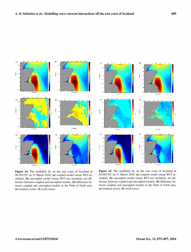
components of the storm were analysed. First, the surge wavegenerated by the minimum of pressure above the North Seawas studied. Figure 13 shows the difference between the to-tal water level and the water level due to tides at 02:00 UTCon 31 March 2015. The model predicted a surge wave up to0.5 m. A comparison between the recorded water level andthe model output showed that the model underestimated thesurge wave by about 0.1 m. The reason for this underestima-tion could be because the boundary conditions for the modelonly included tidal water level and did not include the surgewave from outside the model. The surge wave extended fromthe Firth of Forth southwards: the water level in those re-gions was enhanced by about 0.4–0.5 m. In addition to thesesurge conditions, the Hs of the waves at the same time wasexceeding 7 m in the same areas (see Figures 14 and 15). Fig-ures 11 and 12 show the wave field at two different times inthe storm, at 00:30 and at 02:00 UTC, respectively. The swellwave effect was very low, but contributed to the enhancementof Hs up to 0.5 m, while on the coastline the contribution ofthe WCI was very strong. At 02:00 UTC on 31 March 2010(Fig. 15), when the storm reached the coastline, WCI in-creased Hs by up to 2.5 m in many locations near the Firthof Forth (see Fig. 15d). Figures 14f and 15f show high Hsswell waves at the entrance of the Firth of Forth. These werewaves generated by the large storm shown in Figure 14e, butare no longer influenced by the local wind, but are propagat-



Figure 8. Wave conditions during the 25–26 February 2010 storm:(a) comparison between coupled and uncoupled modelled Hs (m)with observed data in Firth of Forth wave gauge; (b) comparisonbetween coupled and uncoupled modelled Hs (m) in the Aberdeenwave gauge; no observation data were available from this wavegauge during this storm; (c) comparison between coupled and un-coupled modelled Tm (s) with observed data in Firth of Forth wavegauge; (d) comparison between coupled and uncoupled modelledTm (s) in the Aberdeen wave gauge, no observed data were avail-able from this wave gauge during this storm.

ing outside the centre of the windsea waves to the coastline.Hs recorded by the Firth of Forth wave gauge measured apeak of significant wave height of 6.46 m at 05:00 UTC on31 March 2015. The model matched the peak recorded in thewave gauge reasonably well, predicting higher S values ofthe Firth of Forth, where more damages were caused. Thewave–wave interactions due to the interaction between swelland windsea waves was important for the enhancement ofthe Hs in the northern part of the Scotland, where the wind-sea wave conditions were less intense, while the contributionwas low in the central part of the storm.

Figure 9. The modelled Hs on the east coast of Scotland at12:30 UTC on 26 February 2010: (a) coupled model (mean WCIincluded), (b) uncoupled model (mean WCI not included), (c) dif-ference between coupled and uncoupled models, (d) difference be-tween coupled and uncoupled models in the Moray Firth area,(e) windsea waves, (f) swell waves.

3.4.3 The 19 June 2010 storm

The third storm that is considered in this paper was onethat generated high off-shore wave conditions, with swellpropagating to the coastline. This is an example of howthe coupling of swell and windsea waves could lead to ex-treme wave conditions, with significant wave height exceed-ing 6 m offshore and 4–5 m on the coastline. Figure 16 showsthe pressure conditions between 18 and 20 June 2010. On17 June 2010 (not shown) a system of low pressure wasgenerated between Greenland and Iceland. This minimummoved quickly to the Scandinavian peninsula, intensifyingand remaining in the area of Sweden and Norway for 72 h.This low pressure caused strong winds in the northern NorthSea and consequently the generation of waves in the area be-tween the Norway and Scotland. Recorded wave conditionsin the Firth of Forth are compared with the model output(Fig. 17a–c) and model output from the Aberdeen wave rider



Figure 10. The modelled Hs on the east coast of Scotland at19:00 UTC on 26 February 2010: (a) coupled model (mean WCIincluded), (b) uncoupled model (mean WCI not included), (c) dif-ference between coupled and uncoupled models, (d) difference be-tween coupled and uncoupled models in the Moray Firth area,(e) windsea waves, (f) swell waves.

location is shown (Fig. 17b–d). The model demonstrates thewave conditions present during this storm well (both forwave heights and periods) and the results show the limitedeffect of the WCI in those locations. This field of waves ar-rived at the Scottish coastline at the same time as the lowpressure was generating high waves in the bulk of the NorthSea, causing two trains of waves to be in the same placeat the same time. This condition, known as crossing or bi-modal sea, is quite common in the North Sea (Guedes Soares,1984). The model hindcasted that the storm offshore was atits maximum near 16:00 UTC on 19 June 2010 (Fig. 18). At16:00 UTC on 19 June 2010, the modelled offshore, mid-North Sea, windsea-generated waves peaked at Hs ∼ 5 m(Fig. 14e), whereas the swell waves were a little smaller withHs ∼ 3–4 m (Fig. 18f). Further north, in the Moray Firth, theswell waves dominated with the swell having Hs ∼ 6 m andthe windsea having Hs ∼ 2 m. The resulting predicted wavefield had Hs > 6 m (Fig. 18b). In the Moray Firth, an Hs of

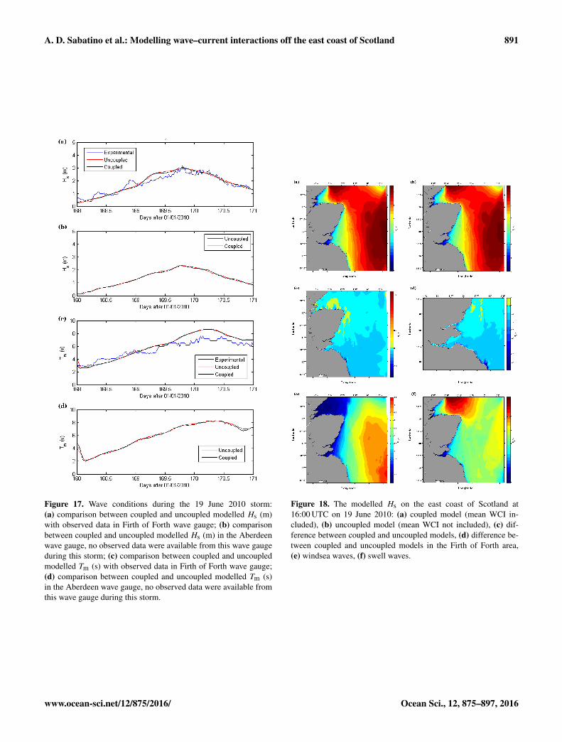
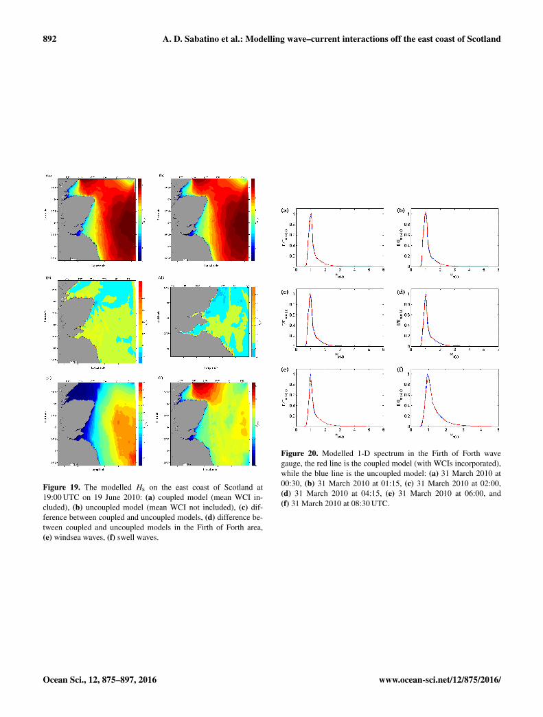
more than 5 m was recorded. However, at this time, the cou-pling between currents and waves caused a decrease of thesignificant wave height at the coastline (Fig. 18c). In somelocations Hs was reduced by more than 0.5 m (see Fig. 18c–d). Three hours later (Fig. 19), the turning tidal currents en-hanced the waves by more than 1.5 m in coastal locations. Inthis storm, the WCIs play a role in the enhancement of thewave conditions: spatially, the effect (Figs. 18–19) is signif-icant on the coastline. In addition, the windsea wave field issignificantly enhanced by swell waves, and the bimodal seaconditions are effective in changing the Hs due to the inter-actions between swell and windsea waves.

3.5 Effect of WCI on the wave spectra

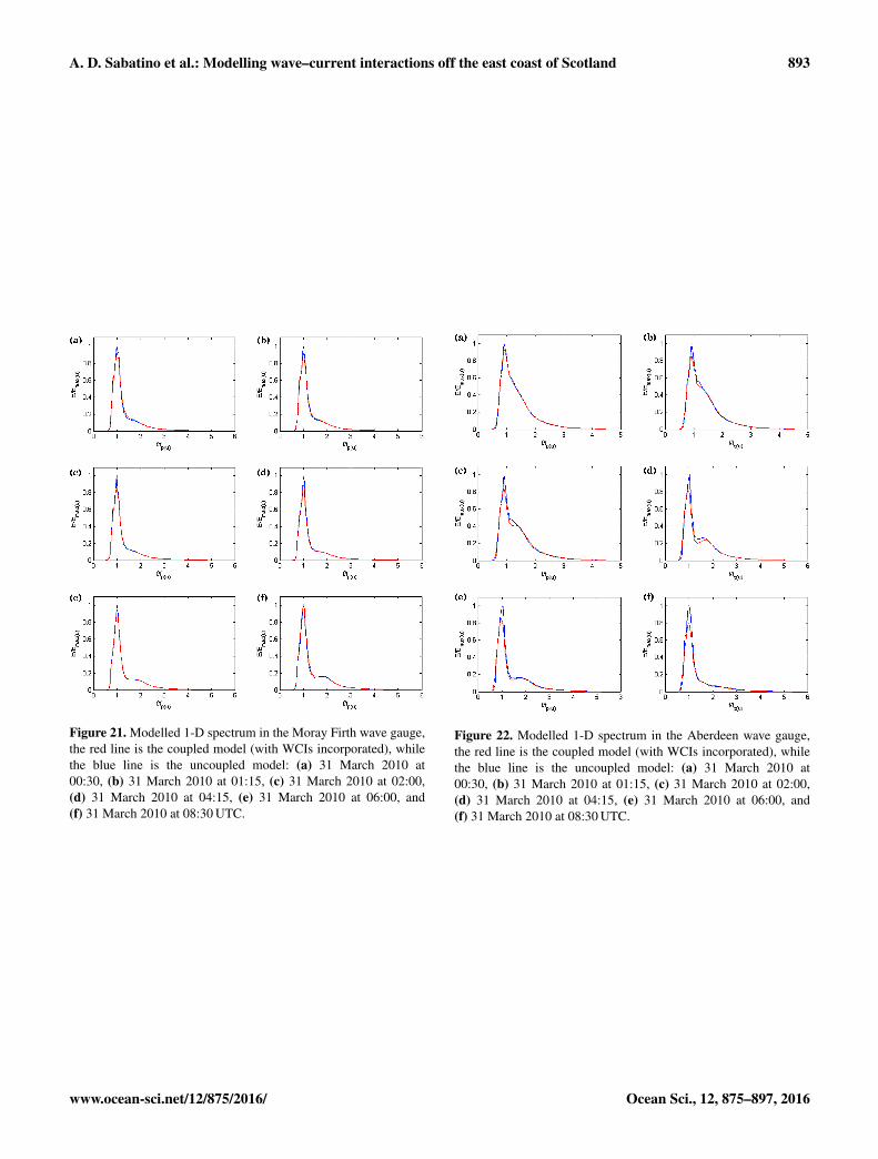
Considering the second storm (30–31 March 2010) we anal-ysed the effect of the WCI on the 1-D and 2-D spectra. Mod-elled spectra were extracted from the model output in threelocations in correspondence with the wave gauges, and theoutput with and without WCIs was analysed (Figs. 20–22).Some significant variation of the energy density of the spec-tra (≈ 20 %) were seen for the considered storm, in particularfor the Aberdeen wave gauge, but also for the Firth of Forthwave gauge, in which high waves were recorded; the majorchanges were reported near the spectral peak. The model alsopredicted a shift of the spectral peak and variation in swellmagnitude. Since large variations were recorded for the Ab-erdeen wave gauge and the Firth of Forth wave gauge, weanalysed the modelled directional spectra with and withoutWCIs for the considered storm. In Figs. 23–24, we show theresults for the 2-D spectrum, in which not only the distribu-tion of the energy with the frequency was shown but also thedistribution with the angle. Variation in the magnitude of thespectral energy with the angle along with small variation inthe direction of the wave train were modelled.

Similar results for the spectrum variations are reported inRusu (2010) for the WCIs at the mouth of Danube, whilesimilar spectral changes were identified in laboratory experi-ments, as in Toffoli et al. (2011b) and Toffoli et al. (2015).

4 Conclusions

In this study we presented a model capable of hindcastingsurge and storms on the east coast of Scotland. The combi-nation of spring tide, strong wind, and high waves can be ex-tremely threatening in coastal areas. The North Sea is one ofthe areas most affected by this forcings. Storms in North Seacan generate extremely high waves as well as rogue waves(Ponce de León and Guedes Soares, 2014).

Results indicate that WCIs play a fundamental role in thewave propagation during severe storms in the coastal areas,while for the open sea, the maximum contribution of thisinteraction is less than 0.5 m of magnitude. The results areconsistent with other studies of WCI in other parts of the



Figure 11. The mean sea level pressure fields (hPa) before and during the 30–31 March 2010 storm.

world, such as in the southern North Sea (Osuna and Mon-baliu, 2004), in which the difference based on the normalizedrms difference of a 1-month period is about 3 % for the Hsand has an rms of 20 % for Tm (Tables 3 and 4 of Osuna andMonbaliu, 2004). Such is the case in the northern AdriaticSea in the shallow areas between the Venetian Lagoon, theGulf of Trieste, and the Istrian peninsula, where deviationsup to 1 m were modelled during bora and sirocco conditions(Benetazzo et al., 2013).

The validation shows that the model performs reasonablywell during both calm periods and storms for waves, and alsoperforms well for tides and surges.

During severe storms, in particular when the low pressurewas over England and Scotland, it was found that the WCIsare significant, causing an increase or decrease inHs that canexceed 2 m in some coastal areas, depending on the directionof the wave field compared to the current. A similar resultwas found for the peak spectral wave period: Fig. 4 showsthat in the time period considered here the largest deviationof wave periods due to WCI is in the estuarine areas of theeast coast, with rms deviations of more than 1.2 s.

Wave propagation in the Firth of Forth during storms gen-erated in the mid-North Sea is driven by trains of swell wavesdetaching from the open sea storm. During the stormy peri-ods considered here, the windsea waves in the Firth of Forth

did not exceed 3.5 m in the outer area of the estuary and 1 min the inner part, while the swell field exceeded 5 m at the en-trance of the Firth of Forth. In the inner firth, the swell waveshave a similar magnitude to the windsea waves. Conversely,the area of the estuary of the Firth of Forth is mainly drivenby locally generated waves. A similar behaviour was noticedin the other two estuarine areas on the east coast: the Tayestuary and the Moray Firth.

The northeast coast of Scotland is more exposed to swellarriving from the North Atlantic and the Norwegian Sea,while the central and southern parts are more exposed to lo-cal windsea waves and to storms generated in the bulk of theNorth Sea.

Spectra were also considered in the analysis of the WCIs:spectral variations, in particular in the energy peak, were sig-nificant and exceeding 20 % in some cases. Wave periods areadequately modelled by the model presented in this paper.Wave models, however, have a large error for the wave pe-riod, since they do not include nonlinear quasi-resonant in-teractions (Onorato et al., 2002; Janssen, 2003; Waseda et al.,2009) that are also fundamental for the correct estimation ofthe Hs when the spectrum is narrow. In addition, wave pe-riods from satellite data are often very difficult to estimate(Gommenginger et al., 2003). Another limitation of the studyis that no surge boundaries were available, so the water level



Figure 12. Modelled currents and waves conditions in the Aberdeenwave gauge location during the 30–31 March 2010 storm (depth ofthe mooring location is 10 m).

and the current fields were only due by tides and the localfield of wind and pressure. This led to an overall underesti-mation of the strength of the current and a possible underes-timation of the total effect of the WCI.

The model also has forecasting capabilities, in particularwhen nested with large-scale models, such as the North At-lantic model (Venugopal and Nemalidinne, 2014, 2015). Alimitation of the model is that the MIKE by DHI softwaredoes not allow an online coupling between waves and tides,slowing the simulation process. In fact, currents and wavesare simulated by different modules and it is not possible toperform a direct coupling. For this work, the currents weresimulated first and then the output data were saved in orderto use them as input for the wave model. Another limita-tion of the model, due to the one-way coupling, is that wecan not study the effect of the wave setup and setdown onthe surge water level (Longuet-Higgins and Stewart, 1962;Bowen et al., 1968), and most importantly, the wave radiationeffect on the current field itself (Bennis et al., 2011; Michaudet al., 2011). Previous work on this interaction shows that themodification of the current field is more important in veryshallow water areas (< 10 m depth). In this paper, however,

Figure 13. The modelled surge wave due to the local wind and pres-sure at 02:00 UTC on 31 March 2010.

we were more interested in the effect of the current field onthe wave. Future work will focus on understanding what ef-fect the waves have on the current dynamics on the east coastof Scotland. This will be implemented by first running thewave model, then using the wave radiation in the hydrody-namic model to estimate the enhancement of the water leveldue to waves near the shoreline and to estimate the variationof the current due to the wave radiation stress.

This research also underlines the importance of high-resolution regional-scale models for the understanding of seadynamics and the forecasting of dangerous sea states: largermodels usually have inadequate resolution to estimate the ef-fect of such processes near the coastline. Future work willbe focused on the hindcasting of freakish wave states basedon the estimation of the kurtosis from the parameters of themodel (Janssen, 2003; Tamura et al., 2009; Ponce de Leónand Guedes Soares, 2014) and on the sediments resuspen-sion in the area of Stonehaven (Heath et al., 2015), which isan intensive study site for suspended sediment and other bi-ological variables in the water column (Serpetti et al., 2011,2012).



Figure 14. The modelled Hs on the east coast of Scotland at00:30 UTC on 31 March 2010: (a) coupled model (mean WCI in-cluded), (b) uncoupled model (mean WCI not included), (c) dif-ference between coupled and uncoupled models, (d) difference be-tween coupled and uncoupled models in the Firth of Forth area,(e) windsea waves, (f) swell waves.

Figure 15. The modelled Hs on the east coast of Scotland at02:00 UTC on 31 March 2010: (a) coupled model (mean WCI in-cluded), (b) uncoupled model (mean WCI not included), (c) dif-ference between coupled and uncoupled models, (d) difference be-tween coupled and uncoupled models in the Firth of Forth area,(e) windsea waves, (f) swell waves.



Figure 16. The mean sea level pressure fields (hPa) before and during the 19 June 2010 storm.



Figure 17. Wave conditions during the 19 June 2010 storm:(a) comparison between coupled and uncoupled modelled Hs (m)with observed data in Firth of Forth wave gauge; (b) comparisonbetween coupled and uncoupled modelled Hs (m) in the Aberdeenwave gauge, no observed data were available from this wave gaugeduring this storm; (c) comparison between coupled and uncoupledmodelled Tm (s) with observed data in Firth of Forth wave gauge;(d) comparison between coupled and uncoupled modelled Tm (s)in the Aberdeen wave gauge, no observed data were available fromthis wave gauge during this storm.

Figure 18. The modelled Hs on the east coast of Scotland at16:00 UTC on 19 June 2010: (a) coupled model (mean WCI in-cluded), (b) uncoupled model (mean WCI not included), (c) dif-ference between coupled and uncoupled models, (d) difference be-tween coupled and uncoupled models in the Firth of Forth area,(e) windsea waves, (f) swell waves.



Figure 19. The modelled Hs on the east coast of Scotland at19:00 UTC on 19 June 2010: (a) coupled model (mean WCI in-cluded), (b) uncoupled model (mean WCI not included), (c) dif-ference between coupled and uncoupled models, (d) difference be-tween coupled and uncoupled models in the Firth of Forth area,(e) windsea waves, (f) swell waves.

Figure 20. Modelled 1-D spectrum in the Firth of Forth wavegauge, the red line is the coupled model (with WCIs incorporated),while the blue line is the uncoupled model: (a) 31 March 2010 at00:30, (b) 31 March 2010 at 01:15, (c) 31 March 2010 at 02:00,(d) 31 March 2010 at 04:15, (e) 31 March 2010 at 06:00, and(f) 31 March 2010 at 08:30 UTC.



Figure 21. Modelled 1-D spectrum in the Moray Firth wave gauge,the red line is the coupled model (with WCIs incorporated), whilethe blue line is the uncoupled model: (a) 31 March 2010 at00:30, (b) 31 March 2010 at 01:15, (c) 31 March 2010 at 02:00,(d) 31 March 2010 at 04:15, (e) 31 March 2010 at 06:00, and(f) 31 March 2010 at 08:30 UTC.

Figure 22. Modelled 1-D spectrum in the Aberdeen wave gauge,the red line is the coupled model (with WCIs incorporated), whilethe blue line is the uncoupled model: (a) 31 March 2010 at00:30, (b) 31 March 2010 at 01:15, (c) 31 March 2010 at 02:00,(d) 31 March 2010 at 04:15, (e) 31 March 2010 at 06:00, and(f) 31 March 2010 at 08:30 UTC.



Figure 23. Polar plot of the modelled 2-D directional spec-trum (energy density, m2

× s / degrees) in the Firth of Forthwave gauge, red indicates the contour plot of the coupled modelspectrum (with WCIs incorporated), while black indicates thecontour plot of the uncoupled model. Contour lines are plot-ted every 0.01 m2 s degrees−1: (a) 31 March 2010 at 00:30,(b) 31 March 2010 at 01:15, (c) 31 March 2010 at 02:00,(d) 31 March 2010 at 04:15, (e) 31 March 2010 at 06:00, and(f) 31 March 2010 at 08:30 UTC.

Figure 24. Polar plot of the modelled 2-D directional spectrum (en-ergy density, m2

× s / degrees) in the Aberdeen wave gauge, red in-dicates the contour plot of the coupled model spectrum (with WCIsincorporated), while black indicates the contour plot of the uncou-pled model. Contour lines are plotted every 0.01 m2 s degrees−1:(a) 31 March 2010 at 00:30, (b) 31 March 2010 at 01:15,(c) 31 March 2010 at 02:00, (d) 31 March 2010 at 04:15,(e) 31 March 2010 at 06:00, and (f) 31 March 2010 at 08:30 UTC.



The Supplement related to this article is available onlineat doi:10.5194/os-12-875-2016-supplement.

Acknowledgements. The authors wish to acknowledge Ian Thurl-beck, Robert Wilson, Alessandra Romanó, Reddy Nemaliddine,Vengatesan Venugopal, Jon Side, Arne Vogler, Ruari MacIver,Simon Waldman, and the two anonymous reviewers for theirhelpful suggestions. The authors are grateful for the financialsupport of the UK Engineering and Physical Sciences ResearchCouncil (EPSRC) through the TeraWatt: Large-scale interactivecoupled 3-D modelling for wave and tidal energy resource andenvironmental impact consortium. The authors are also gratefulto Cefas (UK) for providing satellite and wave gauge data, toThomas O’Donoghue for providing the Aberdeen Bay wavebuoy data, to the British Oceanographic Data Center (BODC)and the Scottish Environmental Protection Agency (SEPA) forthe tide gauge and RCM data, and to the European Centre forMedium-Range Weather Forecasts (ECMWF) for providing windand pressure data.

Edited by: A. Sterl

References

Adcock, T., Taylor, P., Yan, S., Ma, Q., and Janssen, P.: Did theDraupner wave occur in a crossing sea?, P. Roy. Soc. Lond. A-Conta., 467, 3004–3021, 2011.

Adcock, T. A., Draper, S., Houlsby, G. T., Borthwick, A. G., andSerhadlıoglu, S.: The available power from tidal stream turbinesin the Pentland Firth, P. Roy. Soc. Lond. A Mat., 469, 20130072,doi:10.1098/rspa.2013.0072, 2013.

Baston, S. and Harris, R.: Modelling the hydrodynamic characteris-tics of tidal flow in the Pentland Firth, EWTEC 2011, Southamp-ton, UK, 5–9 September 2011, 2011.

Battjes, J.: Surf similarity, Coast. Eng. Proc., 1, 466–480, 1974.Battjes, J. and Janssen, J.: Energy loss and set-up due to breaking of

random waves, Coast. Eng. Proc., 1, 569–587, 1978.Battjes, J. and Stive, M.: Calibration and verification of a dissipation

model for random breaking waves, J. Geophys. Res.-Ocean., 90,9159–9167, 1985.

Benetazzo, A., Carniel, S., Sclavo, M., and Bergamasco, A.: Wave–current interaction: Effect on the wave field in a semi-enclosedbasin, Ocean Model., 70, 152–165, 2013.

Benjamin, B. T. and Feir, J.: The disintegration of wave train ondeep water, J. Fluid Mech., 27, 417–430, 1967.

Bennis, A.-C., Ardhuin, F., and Dumas, F.: On the coupling of waveand three-dimensional circulation models: Choice of theoreticalframework, practical implementation and adiabatic tests, OceanModel., 40, 260–272, 2011.

Berrisford, P., Kållberg, P., Kobayashi, S., Dee, D., Uppala, S., Sim-mons, A., Poli, P., and Sato, H.: Atmospheric conservation prop-erties in ERA-Interim, Q. J. Roy. Meteor. Soc., 137, 1381–1399,2011.

Bowen, A. J., Inman, D. L., and Simmons, V. P.: Wave set-downand set-Up, J. Geophys. Res., 73, 2569–2577, 1968.

Bresnan, E., Hay, S., Hughes, S., Fraser, S., Rasmussen, J., Webster,L., Slesser, G., Dunn, J., and Heath, M.: Seasonal and interannualvariation in the phytoplankton community in the north east ofScotland, J. Sea Res., 61, 17–25, 2009.

Bretherton, F. P. and Garrett, C. J.: Wavetrains in inhomogeneousmoving media, P. R. Soc. Lond. A Mat., 302, 529–554, 1968.

Bryden, I. G. and Couch, S. J.: ME1 – marine energy extraction:tidal resource analysis, Renew. Energ., 31, 133–139, 2006.

Cavaleri, L., Bertotti, L., Torrisi, L., Bitner-Gregersen, E., Serio,M., and Onorato, M.: Rogue waves in crossing seas: the LouisMajesty accident, J. Geophys. Res.-Ocean., 117, 1–8, 2012.

Chawla, A. and Kirby, J. T.: Experimental study of wave breakingand blocking on opposing currents, Coast. Eng. Proc., 1, 759–772, 1998.

Chawla, A. and Kirby, J. T.: Monochromatic and random wavebreaking at blocking points, J. Geophys. Res.-Ocean., 107, 4–1,2002.

Codiga, D. L.: Unified tidal analysis and prediction using the UTideMatlab functions, Graduate School of Oceanography, Universityof Rhode Island Narragansett, RI, 2011.

Davies, A., Sauvel, J., and Evans, J.: Computing near coastal tidaldynamics from observations and a numerical model, Cont. ShelfRes., 4, 341–366, 1985.

Deardorff, J.: On the magnitude of the subgrid scale eddy coeffi-cient, J. Comput. Phys., 7, 120–133, 1971.

Dee, D., Uppala, S., Simmons, A., Berrisford, P., Poli, P.,Kobayashi, S., Andrae, U., Balmaseda, M., Balsamo, G., Bauer,P., et al.: The ERA-Interim reanalysis: Configuration and perfor-mance of the data assimilation system, Q. J. Roy. Meteor. Soc.,137, 553–597, 2011.

DHI: MIKE 3 Hydrodynamics User Manual, vol. 1, 2011a.DHI: MIKE 21 Wave modelling User Manual, vol. 1, 2011b.Dietrich, G.: Die natürlichen Regionen von Nord-und Ostsee auf

hydrographischer Grundlage, Kieler Meeresforsch, 7, 35–69,1950.

Donelan, M. A., Hamilton, J., and Hui, W.: Directional spectra ofwind-generated waves, Philosophical Transactions of the RoyalSociety of London A: Mathematical, Phys. Eng. Sci., 315, 509–562, 1985.

Drennan, W. M., Graber, H. C., Hauser, D., and Quentin, C.: Onthe wave age dependence of wind stress over pure wind seas, J.Geophys. Res.-Ocean., 108, 1–13, 2003.

Earle, M.: Development of algorithms for separation of sea andswell, National Data Buoy Center Tech Rep MEC-87-1, Han-cock County, 53, 1–53, 1984.

Egbert, G. D., Erofeeva, S. Y., and Ray, R. D.: Assimilation of al-timetry data for nonlinear shallow-water tides: Quarter-diurnaltides of the Northwest European Shelf, Cont. Shelf Res., 30, 668–679, 2010.

Eldeberky, Y. and Battjes, J.: Parameterization of triad interactionsin wave energy models, Coast. Dynam., 140–148, 1995.

Eldeberky, Y. and Battjes, J. A.: Spectral modeling of wave break-ing: application to Boussinesq equations, J. Geophys. Res.-Ocean., 101, 1253–1264, 1996.

Ferziger, J. H. and Peric, M.: Computational methods for fluid dy-namics, vol. 3, Springer Berlin, 2002.

Flather, R.: Estimates of extreme conditions of tide and surge usinga numerical model of the north-west European continental shelf,Estuarine, Coast. Shelf Sci., 24, 69–93, 1987.


http://dx.doi.org/10.5194/os-12-875-2016-supplement

http://dx.doi.org/10.1098/rspa.2013.0072


Gommenginger, C., Srokosz, M., Challenor, P., and Cotton, P.: Mea-suring ocean wave period with satellite altimeters: A simple em-pirical model, Geophys. Res. Lett., 30, 1–5, 2003.

Guedes Soares, C.: Representation of double-peaked sea wave spec-tra, Ocean Eng., 11, 185–207, 1984.

Hasselmann, K.: On the spectral dissipation of ocean waves due towhite capping, Bound.-Lay. Meteorol., 6, 107–127, 1974.

Haver, S.: A possible freak wave event measured at the Draupnerjacket 1 January 1995, Rogue waves 2004, 1–8, 2004.

Hearn, C., Hunter, J., and Heron, M.: The effects of a deep chan-nel on the wind-induced flushing of a shallow bay or harbor, J.Geophys. Res.-Ocean., 92, 3913–3924, 1987.

Heath, M. R., Sabatino, A. D., Serpetti, N., and O’Hara Murray,R.: Scoping the impact tidal and wave energy extraction on sus-pended sediment concentrations and underwater light climate,TeraWatt Position Papers, MASTS, 2015.

Huthnance, J.: Physical oceanography of the North Sea, Ocean andShoreline Management, Environment and Sea Use Planning, 16,199–231, 1991.

Janssen, P. A. E. M.: Nonlinear four-wave interaction and freakwaves, J. Phys. Oceanogr., 33, 863–884, 2003.

Johnson, H. K. and Kofoed-Hansen, H.: Influence of bottom frictionon sea surface roughness and its impact on shallow water windwave modeling, J. Phys. Oceanogr., 30, 1743–1756, 2000.

Kaminsky, G. M. and Kraus, N. C.: Evaluation of depth-limitedwave breaking criteria, in: Ocean Wave Measurement and Anal-ysis, 180–193, ASCE, 1993.

Komen, G. J., Cavaleri, L., Donelan, M., Hasselmann, K., Hassel-mann, S., and Janssen, P.: Dynamics and modelling of oceanwaves, Cambridge university press, 1996.

Lavrenov, I.: The wave energy concentration at the Agulhas currentoff South Africa, Nat. Hazards, 17, 117–127, 1998.

Lavrenov, I. and Porubov, A.: Three reasons for freak wave gen-eration in the non-uniform current, Eur. J. Mech. B-Fluid., 25,574–585, 2006.

Lilly, D.: On the application of the eddy viscosity concept in the in-ertial sub-range of turbulence, NCAR Manuscript No. 123, Na-tional Center for Atmospheric Research, Boulder, CO, 1966.

Longuet-Higgins, M. S. and Stewart, R. W.: Radiation stress andmass transport in gravity waves, with application to “surf beats”,J. Fluid Mech., 13, 481–504, 1962.

Ma, Y., Ma, X., Perlin, M., and Dong, G.: Extreme waves generatedby modulational instability on adverse currents, Phys. Fluids, 25,114109, doi:10.1063/1.4832715, 2013.

Mallory, J.: Abnormal waves on the southeast coast of South Africa,Int. Hydrogr. Rev., 51, 99–129, 1974.

Michaud, H., Marsaleix, P., Leredde, Y., Estournel, C., Bourrin, F.,Lyard, F., Mayet, C., and Ardhuin, F.: Three-dimensional mod-elling of wave-induced current from the surf zone to the innershelf, Ocean Sci., 8, 657–681, doi:10.5194/os-8-657-2012, 2012.

Nelson, R. C.: Design wave heights on very mild slopes-an experi-mental study, Transactions of the Institution of Engineers, Aus-tralia, Civil Eng., 29, 157–161, 1987.

Nelson, R. C.: Depth limited design wave heights in very flat re-gions, Coast. Eng., 23, 43–59, 1994.

Nikuradse, J.: Strömungsgestze in rauhen Rohren, 1933.Onorato, M., Osborne, A. R., and Serio, M.: Extreme wave events

in directional, random oceanic sea states, Phys. Fluids, 14, L25–L28, 2002.

Onorato, M., Osborne, A., and Serio, M.: Modulational in-stability in crossing sea states: A possible mechanism forthe formation of freak waves, Phys. Rev. Lett., 96, 014503,doi:10.1103/PhysRevLett.96.014503, 2006.

Onorato, M., Proment, D., and Toffoli, A.: Freak waves in crossingseas, Eur. Phys. J.-Spec. Top., 185, 45–55, 2010.

Onorato, M., Proment, D., and Toffoli, A.: Triggering roguewaves in opposing currents, Phys. Rev. Lett., 107, 184502,doi:10.1103/PhysRevLett.107.18450, 2011.

Osuna, P. and Monbaliu, J.: Wave–current interaction in the South-ern North Sea, J. Mar. Syst., 52, 65–87, 2004.

Otto, L., Zimmerman, J., Furnes, G., Mork, M., Saetre, R., andBecker, G.: Review of the physical oceanography of the NorthSea, Neth. J. Sea Res., 26, 161–238, 1990.

Phillips, O. M.: The Dynamics of the Upper Ocean, 2. Edition,Cambridge-London-New York-Melbourne, Cambridge Univer-sity Press, 1977.

Ponce de León, S. and Guedes Soares, C.: Extreme wave parametersunder North Atlantic extratropical cyclones, Ocean Model., 81,78–88, 2014.

Proudman, J. and Doodson, A. T.: The Principal Constituent of theTides of the North Sea, Philosophical Transactions of the RoyalSociety of London. Series A, Containing Papers of a Mathemat-ical or Physical Character, 224, 185–219, 1924.

Ris, R. and Holthuijsen, L.: Spectral modelling of current inducedwave-blocking, Coast. Eng. Proc., 1, 1247–1254, 1996.

Rusu, E.: Modelling of wave–current interactions at the mouths ofthe Danube, J. Mar. Sci. Technol., 15, 143–159, 2010.

Sabatino, A. D. and Serio, M.: Experimental investigation on statis-tical properties of wave heights and crests in crossing sea condi-tions, Ocean Dynam., 65, 707–720, 2015.

Serpetti, N., Heath, M., Armstrong, E., and Witte, U.: Blending sin-gle beam RoxAnn and multi-beam swathe QTC hydro-acousticdiscrimination techniques for the Stonehaven area, Scotland,UK, J. Sea Res., 65, 442–455, 2011.

Serpetti, N., Heath, M., Rose, M., and Witte, U.: High resolutionmapping of sediment organic matter from acoustic reflectancedata, Hydrobiologia, 680, 265–284, 2012.

Shields, M. A., Dillon, L. J., Woolf, D. K., and Ford, A. T.: Strategicpriorities for assessing ecological impacts of marine renewableenergy devices in the Pentland Firth (Scotland, UK), Mar. Policy,33, 635–642, 2009.

Shields, M. A., Woolf, D. K., Grist, E. P., Kerr, S. A., Jackson, A.,Harris, R. E., Bell, M. C., Beharie, R., Want, A., Osalusi, E.,Gibb, S. W., and Side, J.: Marine renewable energy: The eco-logical implications of altering the hydrodynamics of the marineenvironment, Ocean Coast. Manage., 54, 2–9, 2011.

Shrira, V. and Slunyaev, A.: Nonlinear dynamics of trapped waveson jet currents and rogue waves, Phys. Rev. E, 89, 041002,doi:10.1103/PhysRevE.89.041002, 2014.

Signell, R. P., Beardsley, R. C., Graber, H., and Capotondi, A.:Effect of wave-current interaction on wind-driven circulationin narrow, shallow embayments, J. Geophys. Res.-Ocean., 95,9671–9678, 1990a.

Signell, R. P., Beardsley, R. C., Graber, H. C., and Capotondi, A.:Effect of Wave Current Interaction on Wind Driven CirculationIn Narrow Shallow Embayments, J. Geophys. Res., 95, 9671–9678, 1990b.


http://dx.doi.org/10.1063/1.4832715

http://dx.doi.org/10.5194/os-8-657-2012

http://dx.doi.org/10.1103/PhysRevLett.96.014503

http://dx.doi.org/10.1103/PhysRevLett.107.18450

http://dx.doi.org/10.1103/PhysRevE.89.041002


Smagorinsky, J.: General circulation experiments with the primitiveequations: I. The basic experiment, Mon. Weather Rev., 91, 99–164, 1963.

Song, Y. and Haidvogel, D.: A semi-implicit ocean circulationmodel using a generalized topography-following coordinate sys-tem, J. Comput. Phys., 115, 228–244, 1994.

Stive, M.: A scale comparison of waves breaking on a beach, Coast.Eng., 9, 151–158, 1985.

Tamura, H., Waseda, T., and Miyazawa, Y.: Freakish sea state andswell-windsea coupling: Numerical study of the Suwa-Maru in-cident, Geophys. Res. Lett., 36, 1–5, 2009.

Toffoli, A., Bitner-Gregersen, E., Osborne, A., Serio, M., Mon-baliu, J., and Onorato, M.: Extreme waves in random crossingseas: Laboratory experiments and numerical simulations, Geo-phys. Res. Lett., 38, 1–5, 2011a.

Toffoli, A., Cavaleri, L., Babanin, A., Benoit, M., Bitner-Gregersen,E., Monbaliu, J., Onorato, M., Osborne, A., and Stansberg, C.:Occurrence of extreme waves in three-dimensional mechanicallygenerated wave fields propagating over an oblique current, Nat.Hazards Earth Syst. Sci., 11, 895–903, doi:10.5194/nhess-11-895-2011, 2011b.

Toffoli, A., Waseda, T., Houtani, H., Kinoshita, T., Collins, K.,Proment, D., and Onorato, M.: Excitation of rogue waves ina variable medium: An experimental study on the interac-tion of water waves and currents, Phys. Rev. E., 87, 051201,doi:10.1103/PhysRevE.87.051201, 2013.

Toffoli, A., Waseda, T., Houtani, H., Cavaleri, L., Greaves, D., andOnorato, M.: Rogue waves in opposing currents: an experimentalstudy on deterministic and stochastic wave trains, J. Fluid Mech.,769, 277–297, 2015.

Tolman, H. L.: Effects of tides and storm surges on North Sea windwaves, J. Phys. Oceanogr., 21, 766–781, 1991.

Toro, E. F.: Riemann solvers and numerical methods for fluid dy-namics: a practical introduction, Springer Science & BusinessMedia, 2009.

Venugopal, V. and Nemalidinne, R.: Marine Energy Resource As-sessment for Orkney and Pentland Waters With a CoupledWave and Tidal Flow Model, in: ASME 2014 33rd Interna-tional Conference on Ocean, Offshore and Arctic Engineering,V09BT09A010, American Society of Mechanical Engineers,2014.

Venugopal, V. and Nemalidinne, R.: Wave resource assessment forScottish waters using a large scale North Atlantic spectral wavemodel, Renew. Energ., 76, 503–525, 2015.

Waseda, T., Kinoshita, T., and Tamura, H.: Interplay of resonantand quasi-resonant interaction of the directional ocean waves, J.Phys. Oceanogr., 39, 2351–2362, 2009.

Waseda, T., Hallerstig, M., Ozaki, K., and Tomita, H.: Enhancedfreak wave occurrence with narrow directional spectrum in theNorth Sea, Geophys. Res. Lett., 38, 1–6, 2011.

Whewell, W.: Essay towards a First Approximation to a Map ofCotidal Lines, Philos. T. Roy. Soc. Lond., 3, 188–190, 1830.

Woolf, D. K., Challenor, P., and Cotton, P.: Variability and pre-dictability of the North Atlantic wave climate, J. Geophys. Res.-Ocean., 107, 9–1, 2002.

Xie, L., Liu, H., and Peng, M.: The effect of wave–current inter-actions on the storm surge and inundation in Charleston Harborduring Hurricane Hugo 1989, Ocean Model., 20, 252–269, 2008.

Young, I. R.: Wind generated ocean waves, vol. 2, Elsevier, 1999.


http://dx.doi.org/10.5194/nhess-11-895-2011

http://dx.doi.org/10.5194/nhess-11-895-2011

http://dx.doi.org/10.1103/PhysRevE.87.051201

Documents

Modelling wave–current interactions off the east coast … A. D. Sabatino et al.: Modelling wave–current interactions off the east coast of Scotland study carried out byTolman(1991)