Modelling Wave Propagation in Two-dimensional Structures

using a Wave/Finite Element Technique

E. Manconi and B.R. Mace

ISVR Technical Memorandum 966

February 2007

SCIENTIFIC PUBLICATIONS BY THE ISVR

Technical Reports are published to promote timely dissemination of research results by ISVR personnel. This medium permits more detailed presentation than is usually acceptable for scientific journals. Responsibility for both the content and any opinions expressed rests entirely with the author(s). Technical Memoranda are produced to enable the early or preliminary release of information by ISVR personnel where such release is deemed to the appropriate. Information contained in these memoranda may be incomplete, or form part of a continuing programme; this should be borne in mind when using or quoting from these documents. Contract Reports are produced to record the results of scientific work carried out for sponsors, under contract. The ISVR treats these reports as confidential to sponsors and does not make them available for general circulation. Individual sponsors may, however, authorize subsequent release of the material. COPYRIGHT NOTICE (c) ISVR University of Southampton All rights reserved. ISVR authorises you to view and download the Materials at this Web site ("Site") only for your personal, non-commercial use. This authorization is not a transfer of title in the Materials and copies of the Materials and is subject to the following restrictions: 1) you must retain, on all copies of the Materials downloaded, all copyright and other proprietary notices contained in the Materials; 2) you may not modify the Materials in any way or reproduce or publicly display, perform, or distribute or otherwise use them for any public or commercial purpose; and 3) you must not transfer the Materials to any other person unless you give them notice of, and they agree to accept, the obligations arising under these terms and conditions of use. You agree to abide by all additional restrictions displayed on the Site as it may be updated from time to time. This Site, including all Materials, is protected by worldwide copyright laws and treaty provisions. You agree to comply with all copyright laws worldwide in your use of this Site and to prevent any unauthorised copying of the Materials.

UNIVERSITY OF SOUTHAMPTON

INSTITUTE OF SOUND AND VIBRATION RESEARCH

DYNAMICS GROUP

Modelling Wave Propagation in Two-dimensional Structures Using a Wave/Finite Element Technique

by

E. Manconi and B.R. Mace

ISVR Technical Memorandum No: 966

February 2007

Authorised for issue by Professor M.J. Brennan

Group Chairman

© Institute of Sound & Vibration Research

Abstract

The purpose of this work is to present a general method for the numerical analysis of wavepropagation in 2-dimensional structures by the use of a finite element method (FEM). Themethod involves typically just one finite element to which periodicity conditions are appliedinstead of modelling the whole structure, thus reducing drastically the cost of calculations. Themass and stiffness matrices are found using conventional FE software. The low order dynamicstiffness matrix so obtained is post-processed and the wavenumbers and the frequencies thenfollow from various resulting eigenproblems.The method is described and numerical examples given. These include isotropic and orthotropicplates, isotropic cylindrical shells and the more complex case of sandwich cylindrical shells forwhich analytical solutions are not available. The last two cases are studied by postprocessingan ANSYS FE model.The main advantage of the technique is its flexibility since standard FE routines can be usedand therefore a wide range of structural configurations can be easily analysed. Moreover thepropagation constants for plane harmonic waves can be easily predicted for different propagationdirections along the structure. The method is seen to give accurate predictions at negligiblecomputational cost.

1

Contents

1 Introduction 3

2 The Wave–FE method 62.1 Finite element analysis of 2-dimensional structures . . . . . . . . . . . . . . . . . 62.2 Wave propagation in 2-dimensional uniform structures . . . . . . . . . . . . . . 72.3 Periodicity conditions . . . . . . . . . . . . . . . . . . . . . . . . . . . . . . . . . 92.4 Real propagation constants . . . . . . . . . . . . . . . . . . . . . . . . . . . . . . 92.5 Complex propagation constants . . . . . . . . . . . . . . . . . . . . . . . . . . . 9

3 Plane wave propagation in plates 123.1 Isotropic plate . . . . . . . . . . . . . . . . . . . . . . . . . . . . . . . . . . . . . 12

3.1.1 Real–valued dispersion curves and wave forms . . . . . . . . . . . . . . . 123.1.2 Accuracy . . . . . . . . . . . . . . . . . . . . . . . . . . . . . . . . . . . . 163.1.3 Complex–valued propagation constants . . . . . . . . . . . . . . . . . . . 183.1.4 Sensitivity analysis of eigenvalues . . . . . . . . . . . . . . . . . . . . . . 193.1.5 Sensitivity analysis of the wavenumbers . . . . . . . . . . . . . . . . . . . 20

3.2 Orthotropic plate . . . . . . . . . . . . . . . . . . . . . . . . . . . . . . . . . . . 233.2.1 Real–valued dispersion curves . . . . . . . . . . . . . . . . . . . . . . . . 233.2.2 Complex–valued propagation constants . . . . . . . . . . . . . . . . . . . 26

4 Wave propagation in curved and cylindrical shells 274.1 Isotropic shell . . . . . . . . . . . . . . . . . . . . . . . . . . . . . . . . . . . . . 294.2 Sandwich shell . . . . . . . . . . . . . . . . . . . . . . . . . . . . . . . . . . . . . 36

5 Concluding remarks 40

2

1. Introduction

One of the most general approximate methods for solving problem concerning the dynamicsof continuous structures is the finite element method (FEM). In its “classical” modal/dynamicapplication, this method is used to obtain information about the vibrational behaviour fromthe model of the whole structure in the low frequency range. However, in many engineeringapplications, high frequency vibrations become significant, in particular where sound transmis-sion have to be considered. At high frequencies, when the wavelengths become very small, theuse of this approach may become inappropriate because the size of the FE model that canpredict response accurately becomes too large and therefore computationally very expensive.Furthermore, numerical inaccuracies arise at higher frequencies. One of the main reasons is thedispersion error involved in the FE approximation. The dispersion error refers to the differencebetween the numerical estimates of the wavenumbers and the true values. Since this errorincreases with the frequency, in order to keep it within “acceptable” limits, the FE model sizehas to be increased leading to a drastic increase in the computer time and storage. Therefore,at high frequencies, a detailed FE model may be very difficult to solve or perhaps impossiblesometimes. One alternative technique to FEM is Statistical Energy Analysis (SEA). It is mainlyused for structures that can be considered as an assemblage of subsystems. The application ofSEA requires the knowledge of the modal density and of the relation between modal energy andvibration velocity for each subsystem. However, while for simple structures these characteris-tics are well known, for complex structures the analysis is often very difficult. Computationaltechniques such as spectral FEM or the technique proposed in the present report can be usedto evaluate these quantities.Another approach to obtain information about vibration of structures is the Dynamic StiffnessMethod, DSM, sometimes also termed Spectral Element Method when it is applied to waveg-uides, [6, 7]. The method divides the structure into simple elements whose degrees of freedomare defined at certain points called nodes. The key of this technique is the establishment of adynamic stiffness matrix in the frequency domain to relate nodal responses x and the forces F,i.e.

D(ω)x = F.

Only one element has to be analysed and a global dynamic stiffness matrix can be subsequentlydefined by assembly in a similar manner to FEM. Since the matrix D is obtained from the exactsolutions of the differential equation of motion, the method describes exactly the behaviour ofthe element but it can only be applied to relatively simple cases. Flotow, [8], and Beale andAccorsi, [9], applied these ideas to study the vibrations of network structures composed of simplebeam elements. They analysed the dynamics of the structure in terms of wave propagation ina single beam element. Hence, they solved for the dynamics of the whole structures takinginto account the boundary conditions between every single element and those for the wholestructure. Although the method that they proposed reduces the calculation cost greatly, it isdeveloped for a particular class of structures like frame structures.A large amount of research has focused on the question of extending the range of frequencyapplication of the FEM. In this context one method for structural dynamics and acousticapplications is the spectral finite element method (SFEM). The SFEM strategy applies tostructures that present symmetry in one direction, called a waveguide. The name is due tothe fact that they allow waves to propagate in the direction of the axis of symmetry of thestructure. As it will be described later they are a particular case of periodic structures.

3

The basic steps of the SFEM are described in [1]. The SFEM uses the FEM to describe thecross–section motion. At the same time the nodal displacements along the axis with whichthe structure is aligned are in effect assumed to be harmonic functions of space. For harmonicvibrations, the solutions to the wave equation are given by a polynomial eigenvalue problem.These basic assumptions have been used by several authors to describe wave propagation indifferent kinds of waveguide structures. Some examples include the paper by Gavric whoapplied the method to a railway track, [2], Finnveden, who studied rib-stiffened structures andfluid-filled pipes, [3, 4] and Shorter who developed SFE for viscoelastic laminates, [5].Other authors have proposed a different technique to analyse wave propagation in periodicstructures. The term “periodic structures” indicates structures which exhibit characteristicsthat repeat periodically in one, two or three-dimensions. In other words, a periodic structurecan be considered as an assemblage of identical elements, called cells or periods, which arecoupled to each other on all sides and corners by identical junctions. This characteristic isindeed observable in many real systems. Examples include railway tracks, flat or curved panelsregularly supported, such as stringer stiffened panels, fluid filled pipes with flanges, acousticalducts, rail structures, car tyres, composite plates or shells etc. The use of the structures pe-riodicity can be exploited to solve dynamic problem with reduced computational cost. Manyprevious works have concerned periodic structures. One of the classical books where the math-ematics of wave propagation in periodic structures has been discussed is that of Brillouin [10].More recent works, [11–15], have studied the problem of defining the dynamical behaviour ofperiodic structures considering the properties of its characteristic waves. These works considerstructures with cross–sectional properties that are uniform along one direction. Much attentionis focused on uniform plates and shells with identical stiffeners at regular intervals. In partic-ular in [12] a finite element approach is used for obtaining the dispersion curve of a periodicstructure. The main idea is to relate the displacements, q, and the forces, f, at the left andthe right hand–side of a periodic element of the structure by the propagation constant λ in thefollowing way:

qR = λqL, fR = −λfL,

where λ = eiµ, µ is the propagation constant and i =√−1.

Following this idea, in [16–18], an estimate of the wave motion along a uniform waveguideis carried out by considering a transfer matrix to relate the displacements and the forces onboth left and right hand–sides of a section of the waveguide. The transfer matrix is the resultof a manipulation of the mass and stiffness matrices obtained from a conventional FE modelof a small section of the waveguide. In this Wave–FE (WFE) approach, wave propagation isdescribed in terms of eigenvalues and eigenvectors of this matrix and the dispersion relationis obtained via a standard eigenvalue problem. In particular, in [16], after reformulating thedynamic stiffness matrix of one cell of a waveguide in terms of wave propagation, the dynamicstiffness matrix of the whole structure is built using periodic structure theory. The response ofthe whole structure can then be evaluated simply. The two examples provided in [16], beamsand plates excited by a point force, have shown that the accuracy of the method is good whencommon requirements for FE discretisation are satisfied, that is, the length of the element issmall enough compared to the wavelength. In the same way as the SFEM, the advantage ofthis strategy is that only one section of the structure has to be meshed and solved, reducingdrastically the cost of calculation. However, unlike the SFEM, the method described earlierexploits the high geometrical and material flexibility of standard commercial FE packages toextract the stiffness, mass and damping matrices. This is a great advantage since no newelements have to be developed for each application. Furthermore, the SFEM method cannot

4

be applied to 2-dimensional structure.The purpose of this work is to extend the WFE approach to 2-dimensional structures. Theadvantages in extending the method to the 2-dimensional case consists mostly of the fact thatonly one finite element can be used and that the propagation constants of plane harmonicwaves can be easily evaluated for different propagation direction across the structure. Animportant reference for this work is [19], where FEM is applied to model generic periodicstructures. Herein, a general method is presented that enables vibrational waves propagatingin a periodic 2-dimensional structure to be analysed by the use of a finite element method.Similar to the approach presented in [16–18], this method relates the right-left and the top-bottom displacements and generalised forces of one rectangular element by

qR = λxqL, fR = −λxfL,

qT = λyqB, fT = −λyfB,

where λx = eiµx , λy = eiµy and µx, µy are the propagation constants of a plane harmonic wave ina 2-dimensional geometry. Making use of the FEM, the mass and stiffness matrices are obtainedand they are subsequently post-processed in order to obtain a problem whose eigenvalues andeigenvectors describe the wave propagation characteristics. Special attention is given to thiseigenvalue problem. In fact if µx and µy are assigned, the frequencies of wave propagationcan be obtained from a standard eigenvalue problem. On the other hand if the propagationfrequency is prescribed it yields a polynomial or a transcendental eigenvalue problem. Thereal dispersion curves can be easily obtained by solving the first case. The solutions to thetranscendental eigenproblem are less obvious nevertheless, for the more general case of complexpropagation constants, they represent decaying wave motion at a given frequency. For thefirst kind of problem efficient algorithms, which include error and condition estimates, are wellknown while the last problem, which is more general, is less obvious and different methods tosolve it are analysed.This memorandum is organised in three parts. The first part concerns the description of thegeneral method by which the wavenumbers for a 2-dimensional structure can be predicted froma FE model. The second and third parts deal with the application of the method to severalexamples. First an isotropic plate is considered as an illustrative example. Another exampleconcerning an orthotropic plate made of a Glass/Epoxy composite material is discussed. Inthe third part cylindrical shells structures are discussed. In particular an example of a curvedsandwich panel, for which analytical solutions are not available, is provided. The dispersionrelations, the complex propagation constants and wave-forms are given. A sensitivity analysisis also performed in order to identify those results which truly represent the behaviour of thecontinuous structure. Finally the results are discussed and conclusions are drawn.

5

2. The Wave–FE method

In this section a general theoretical approach to apply the wave-FE method to a 2-dimensionalperiodic structure is described. The main idea is to use a wave approach instead of a tradi-tional modal one to describe the vibration behaviour of a uniform structure modelled by a FEtechnique.

2.1. Finite element analysis of 2-dimensional structures

A two dimensional periodic structure can be considered as an assembly of identical elementswhich are coupled to its neighbours on all sides and corners. Every element, or cell, of thesystem can be indicated by two numbers (ni, nj) which defines its position along the directionsd1 and d2 parallel to the direction of the system periodicity as shown in Figure 1. The dynamicalbehaviour of such structures can be studied in a simple way if the behaviour of only one cell isanalysed. The general procedure for FE discretisation of continuous structures is well knownand therefore will not be described here. The cell can be in general represented by a model

d1

d2

n1, n2 n1 + 1, n2n1 − 1, n2

n1, n2 + 1

n1, n2 − 1

Figure 1: Uniform 2-dimensional structure.

with internal and boundary degrees of freedom q. The only condition required for the followinganalysis is that the cell is meshed with an equal number of nodes at its left–right and top–bottom sides. Another requirement for the mesh is a small spatial discretisation comparedwith the wavelength of the problem. As a rule of thumb, 6-10 elements per wavelength have tobe used to obtain accurate results.Using the stiffness and mass matrices obtained from the FE model, the equation of motion forthe cell for time harmonic motion is (

K− ω2M)q = F, (1)

where ω is the angular frequency, K and M are the stiffness and mass matrices, F is the loadingvector containing the nodal loads and q is the vector containing the nodal displacements. It isworth noting that the loading vector F is responsible for transmitting the wave motion fromone element to the next and therefore, even if free wave motion is considered and so no externalloads exist, it is not zero.

6

Lx

z y

x

Ly

3 4

21

Figure 2: Rectangular 2-dimensional element.

Now consider a uniform structure as a special case of a periodic structure. The structureis meshed using conventional FEs and rectangular elements. The smallest cell that can beconsidered in the analysis of the uniform structure is just one FE. It will be shown that, byappropriately formulating the problem, this element is sufficient to estimate the dispersionrelations for the whole system. Figure 2 shows a 2-dimensional rectangular finite element. TheCartesian axes x and y are chosen as the preferred directions d1, d2 respectively. The elementis a rectangular four node element and x, y and z are the global coordinates. The nodes arenumbered as in Figure 2. The displacement vector for the element is q = [q1,q2,q3,q4]

T , whereqi contains the nodal degrees of freedom.

2.2. Wave propagation in 2-dimensional uniform structures

Plane waves propagating in the 2-dimensional structures are considered. Let φ be a genericdisturbance. It will propagate as a harmonic free wave if the physical problem admits a solutionof the type

φ = Aei(ωt−k·r), (2)

where A is a constant, r is a vector with components x and y and k is a vector which representsthe wavenumbers for a wave travelling in the θ direction with respect to the x axis. In thediscrete model of the structure shown in Figure 1, at the points (niLx, njLy),

φni,nj= Aei(ωt−nikxLx−njkyLy) (3)

where kx = k cos(θ), ky = k sin(θ), represent the components of the wavenumber k along the xand y axes and Lx and Ly represent the element lengths. In the following analysis µx = kxLx

and µy = kyLy indicate the propagation constants for the structure while λx and λy equal e−iµx

and e−iµy respectively.The propagation constants are usually complex numbers. The real parts of µx and µy representthe change in phase in the wave motion from one cell to the next, while the imaginary parts ofµx and µy represent the wave attenuation along the x and y directions.For the general case of a system discretised by a certain number of cells, Figure 1, the distur-bance φ propagates through the structure such that

φn1+1,n2 = λxφn1,n2 ; φn1,n2+1 = λyφn1,n2 ; φn1+1,n2+1 = λxλyφn1,n2 . (4)

7

Considering equation (4) for the simple case of one finite element as shown in Figure 2, we canwrite the following relations for the nodal displacements:

q2 = λxq1; q3 = λyq1; q4 = λxλyq1. (5)

Equations (5) can be rearranged to give

q = Qrq1, (6)

whereq = [q1 q2 q3 q4], (7)

andQr = [I λxI λyI λxλyI]T . (8)

Since equilibrium requires that the sum of the nodal forces at each node is zero, at node 1 then

[I −λ−1

x I −λ−1y I (λxλy)

−1I]

F1

F2

F3

F4

= 0. (9)

Hence, premultiplying both side of equation (1) by

Ql = [I λ−1x I λ−1

y I (λxλy)−1I], (10)

the equation of free wave motion takes the form:

[K(µx, µy)− ω2M(µx, µy)]q1 = 0, (11)

whereK = QlKQr,

M = QlMQr

(12)

are the reduced stiffness and mass matrices. K and M are n×n matrices, where n is the numberof nodal degrees of freedom. The elements of these matrices are functions of the propagationconstants and of the elastic and inertial characteristics of the structure.Equation (11) represents an eigenvalue problem in ω2 for given values of µx and µy. Thisequation can also be seen as an eigenvalue problem in µx and µy for a given ω and a givenpropagation direction θ. This is a more general case but less easy to solve since it represents atranscendental eigenvalue problem.It can be seen from equation (11) that the mathematical formulation of the method is fairlysimple and that standard FE packages can be used to obtain the mass and stiffness matrices ofone period of the structures. This is a great advantage because there is no need to create FEelements “ad hoc” every time that a new structure has to be studied.

8

2.3. Periodicity conditions

Equation (11) yields the same values of q and ω for (µx, µy) or (µx + 2m1π, µy + 2m2π) wherem1 and m2 are integers, that is the propagation disturbance and the frequency are periodicfunctions of the propagation constants. This is a consequence of considering a discretisedstructure instead of a continuous one and represents a substantial difference with the standardcontinuum approach. In fact, for the continuous model it is implicitly supposed that a certainpropagation characteristic could be “measured” between particles. Therefore in the continuousmodel the observable wavelengths will be all the ones included in the interval 0 ≤ λ ≤ ∞.On the other hand, since the FE is a discrete model of the structure, if the distance betweenthe nodes along x and y in one element are Lx and Ly, the model will allow any wavelengthcomponents along x and y such that λx ∈ [0, 2Lx], λy ∈ [0, 2Ly], or, in term of the propagationconstants, µx ∈ [0, 2π], µy ∈ [0, 2π]. Since a wave propagates in the positive and negativedirection in the same way, Re(µx) ∈ [−π, π], Re(µy) ∈ [−π, π] are taken as the most convenientinterval in which to examine the variation of ω with respect to the variation of the propagationconstants. This restriction is not so arbitrary as it appears since it contains a complete periodof the frequency and avoid ambiguity in the wavenumbers at the same time. Other “intervals”of the same kind can be found but are not of interest for the present work. Detailed discussionabout the periodicity conditions can be found in [10].

2.4. Real propagation constants

In this section we consider waves that propagate in the 2-dimensional structure without atten-uation. This means that the propagation constants µx and µy are real quantities and for freelypropagating waves in an undamped structure

|λx| = 1, |λy| = 1.

If the wave propagation constants are known, the problem of finding the propagating frequenciesmathematically means solving the standard eigenvalue problem for ω2, equation (11).For real values of µx and µy, Qr = Q∗

l , where ∗ indicates transpose conjugation. Due to the factthat the stiffness and mass matrices in equation (1) are real, symmetric and positive definitematrices, then for real propagation constants

K = QrKQl = Q∗l KQl = [Q∗

l KQl]∗ = K

∗

M = QrMQl = Q∗l MQl = [Q∗

l MQl]∗ = M

∗.

(13)

Hence, the dynamic matrices K and M are positive definite Hermitian matrices. For any givenvalues of the propagation constants there will therefore be n real positive eigenvalues for whichwave propagation is possible. This number is equal to the number of degrees of freedom pernode, n. It should be noted that, there is also a pair of possible waves travelling in the oppositedirection: if (µx, µy) is a solution so is (−µx,−µy).

2.5. Complex propagation constants

Unlike the previous analysis, equation (11) can be formulated also to give the propagationconstants for a given value of ω and θ. Two approaches are discussed to obtain the propagation

9

constants: with the first one the problem is reduced to a standard polynomial eigenvalueproblem while with the second the eigenproblem is a transcendental eigenvalue problem. Forthe first kind of problem efficient algorithms, which include error and condition estimates, arewell known while the second problem, which is more general, is less common and differentmethods can be used to solve it.By partitioning the dynamic stiffness matrix of equation (1) as

D =

D11 D12 D13 D14

D21 D22 D23 D24

D31 D32 D33 D34

D41 D42 D43 D44

,

equation (11) can be rewritten in the form

[(D11 + D22 + D33 + D44) + (D12 + D34)λx + (D21 + D43)λ−1x +

+(D13 + D24)λy + (D31 + D42)λ−1y + D14λxλy + D41λ

−1x λ−1

y +

+D32λxλ−1y + D23λ

−1x λy]q = 0.

(14)

Considering the transpose and the transpose conjugate of equation (14) and exploiting thesymmetry of the dynamic stiffness matrix, it can be easily proved that the eigenvalues of thisproblem occur in pairs (λx, λ

∗x), (λ−1

x , λ−1x

∗) and (λy, λ

∗y), (λ−1

y , λ−1y

∗).

If the ratio µy/µx is a rational number, that is µy/µx = m2/m1, where m1 and m2 are integerswith no common divisors, we can reformulate the propagation constants as µx = m1σ, µy =m2σ. Since λx = e−iµx and λy = e−iµy , equation (14) can be rearranged in this case as

[A0 + A1γm1 + A2γ

m2 + A3γ2m1 + A4γ

2m2 + A5γm1+m2+

+A6γ2m1+m2 + A7γ

m1+2m2 + A8γ2m1+2m2 ]q = 0,

(15)

where γ = e−iσ and the matrices Aj are of the same order as the partitions of D. Equation(15) represents a standard polynomial eigenvalue problem of order n(2m1 + 2m2) and can besolved by efficient algorithms. The eigenvalues of equation (15) are transcendental functionsin the complex variable σ. In this particular formulation, the problem admits an infinity ofperiodic solutions since, if σ is a solution, σ± 2pπ, p integers, is a solution as well. In terms ofthe propagation constants µx and µy, the correspondent periods for the roots of equation (15)will be 2m1π and 2m2π.

In order to consider a general way to solve equation (14) for any possible (irrational) value ofµy/µx we can write, for waves propagating at an angle θ with respect to the x axis

λx = e−ikLx cos(θ),

λy = e−ikLy sin(θ).(16)

This leads to a general formulation of the problem

A(e−ikLx cos(θ), e−ikLy sin(θ))q = 0, (17)

10

where the elements of the matrix A are transcendental functions of the complex variable k fora given value of θ.The analytical functions involved in equation (17), sums and products of exponential functions,are continuous and continuously differentiable with respect to the variable k. Therefore, themost natural technique to solve (17) is to reduce the problem to the transcendental equationg(k) = |A(k)| = 0 and solve it by Newton’s method. Newton’s method seeks the solutions ofthe nonlinear equation by solving iteratively a sequence of linear problems of the form

g(ki−1) + rig′(ki−1) = 0

ki = ki−1 + ri.(18)

Sufficient conditions for the existence of the solution and the convergence of Newton’s methodare given by the Kantorovich Theorem, see [20].A similar way to solve the problem is to use the Newton’s eigenvalue iteration method [21], [22].This method extends Newton’s method to the matrix A(k) in the following way. Given

B = −dA(k)

dk,

then solve for[A(ki−1)− ri(B(ki−1)]qi = 0,

ki = ki−1 + min(ri),(19)

where min means the minimum absolute value of the eigenvalues ri. The main difference withthe same method applied to the one-dimensional case is that the values of ri are determinedby solving an eigenvalue problem and the approach is more general. Although both problemsconsider first order approximations, higher order approximations can be included by consideringhigher order terms in the series expansion of either the matrix A or of the function g.An alternative choice seeks the complex roots of the equation |A| = 0 using a variant of thePowell Method, [23]. This algorithm is implemented in the function fsolve in the OptimizationToolbox of MATLAB as a default choice.The solutions obtained by applying the three different methods are virtually identical but thefunction fsolve is computationally more efficient than the other two. Despite the fact that thesolution space is more sensitive to Re(k) than Im(k), the above algorithms used have goodguaranteed convergence within the closed intervals used to find the solutions. Moreover, theobjective function |A| at the estimated solutions k was found to always be very “small”.However two important aspects are still open to discussion: the number of solutions and theinterval in which all these solutions are defined. The choice of this interval is a more interst-ing/relevant problem as all the iterative root–finding methods depend critically on the initialestimates.Alternative numerical approaches for finding complex roots of the transcendental equation (17)may be the Interval Newton method, [24], [25], the contour integration method, [26] or Muller’smethod, [27]. The evaluation and comparison of these methods is object of future work.

11

3. Plane wave propagation in plates

In this section flexural wave motion in a 2–dimensional thin plate is investigated. First anuniform isotropic plate is analysed as an illustrative example. The second part concerns themore complicated and practical case of an orthotropic plate made of Glass/Epoxy compositematerial. The real–valued dispersion curves, the complex propagation constants and accuracyand sensitivity analysis of the results are given. Although the complex propagation constantsfor given frequency and for given propagation direction have been obtained, the procedure thatenables the complete complex–valued dispersion curves to be fully evaluated is in progress.As stated before, only one single finite element is analysed, Figure 2. For a plate in bendingvibration, the element has three degrees of freedom at each node: translation in the z directionand rotations about the x and y axes. The shape function assumed for this element is a completecubic to which the two quadratic terms x3y and xy3 have been added. For more detail see [28].

3.1. Isotropic plate

A steel plate of thickness h located in the (x, y) plane is considered. In the numerical examplesbelow the material properties are taken to be: Young’s modulus E = 19.2 ·1010N/m2, Poisson’sratio ν = 0.3, density ρ = 7800 kg/m3.The governing equation for the out–of–plane motion w of the thin plate is:

D

(∂4w

∂x4+ 2

∂4w

∂x2∂y2+

∂4w

∂y4

)= −ρh

∂2w

∂t2, (20)

whereD =

Eh3

12(1− ν2),

is the flexural rigidity. A nondimensional frequency is defined as

Ω = ωL2x

√ρh/D.

If nothing different is specified the plate element is assumed to be a square element of lengthL. Harmonic wave solutions of the form

w = Aeiωt−ikxx−ikyy (21)

are sought. Substituting (21) into equation (20), gives

D(k2x + k2

y)2 = ρhω2. (22)

Since kx = k cos(θ), ky = k sin(θ), and hence k = k2x + k2

y, the analytical plate free wavenumberis defined as

k =√

w4

√ρh

D. (23)

3.1.1. Real–valued dispersion curves and wave forms

Figure 3 shows the plots of the nondimensional (Ω, µx, µy) surfaces, where µx = kxLx andµy = kyLy for real kx and ky. As expected the surfaces are symmetric with respect to the

12

−1

−0.5

0

0.5

1

−1

−0.5

0

0.5

10

2

4

6

8

10

12

14

16

18

µx/πµ

y/π

Ω1

−1

−0.5

0

0.5

1

−1

−0.5

0

0.5

10

10

20

30

40

50

µx/πµ

y/π

Ω2

−1

−0.5

0

0.5

1

−1

−0.5

0

0.5

115

20

25

30

35

40

45

50

55

60

µx/πµ

y/π

Ω3

Figure 3: Isotropic plate. Propagation surfaces.

13

µx = 0 and µy = 0 planes. This symmetry is due to the isotropy of the plate and due to thefact that a wave propagates in the same way in the positive or in the negative direction. Thewave motion is possible only at the frequencies specified by the surfaces in Figure 3 since atother frequencies the wave decays exponentially. Hence we call these surfaces as passing bandsaccording to Brillouin, [10].In order to highlight some important properties of the wave-FE model, Figure 4 shows thenumerical and analytical dispersion curves for a wave propagating along the x direction. It

−3 −2 −1 −0.62 0 0.62 1 2 30

20

30

40

50

60

µx/π

ΩNumerical. First branchNumerical. Second branchNumerical. Third branchAnalytical

First propagating band

Second propagating band

Third propagating band

Ωa

Ωb

Ωc

Accurate

Figure 4: Real–valued dispersion curves for θ = 0. Numerical and analytical curves.

can be seen that the frequency is periodic with a period 2π. Therefore, as explained in thesection 2.3, it is sufficient to evaluate the variation of the frequency within the interval [−π, π].As expected three passing bands are obtained for the plate because there are three DOFs pernode. However, only the first, which corresponds to the results obtained from the analyticalformulation, exists for the continuous plate and it is the one of interest for the present analysis.The figure shows that the first branch is a good approximation to waves in the continuous plateif the element length is about one-tenth of the wavelength, that is approximately µx < 2π/10.The second and third passing bands are due to the discrete FE model of the plate. It can benoted that in the first passing band the model behaves as a low-pass filter for all the frequenciesbelow the cut-off frequency Ωa. The frequencies outside the passing bands, i.e. Ωa < Ω < Ωb

and Ω > Ωc, do not propagate. Although the presence of the bounding frequencies, Ωa, Ωb andΩc, is due to the discretisation of the continuous model, their evaluation can be of importancesince they are characteristics of the structure. In [13], for example, it has been proved that thebounding frequencies for a 1-dimensional periodic system of symmetric elements, correspondto the characteristic frequencies of the single element with its ends either fixed or free. Other

14

−0.6 −0.4 −0.2 0 0.2 0.4 0.6

−0.6

−0.4

−0.2

0

0.2

0.4

0.6

µx

µ y

200 Hz

800 Hz

1500 Hz

Figure 5: Isotropic plate. Dispersion curves in the (µx, µy) plane. Square element.

considerations about the bounding frequencies can be found in [11], [12], [14].Figures 5 and 6 show the dispersion curves in the (µx, µy) plane for the first propagatingband at different values of the propagation frequency. Two examples are considered. The firstconcerns a square plate element of length L, Figure 5, while the second applies to a rectangularelement for which the distances between the nodes along x and y are taken as Lx = L andLy = 1/2L respectively, Figure 6. Since the plate is isotropic the wavenumber is independentof the propagation direction and, as expected, the contour curves for the square plate elementare circular, Figure 5. On the other hand, the curves in Figure 6 relative to the rectangularelement are ellipses since µy = 1/2kyL and µx = kxL.Some examples are now given in order to show the frequencies, f, and the associated waveforms, V. These result from the eigenproblem defined in equation (11). The waveforms areevaluated for plane waves that propagate in the directions θ = 0 and θ = π/4.Illustrative example 1). Direction of propagation θ = 0, wavenumber 57.86 m−1.From equation 11, the frequencies and the corresponding eigenvectors are:

f =

4002.328 · 105

2.401 · 105

; V =

−0.0173 0 00 0 −0.001 + 0.1i−i −0.001 + 0.1i 0

. (24)

Illustrative example 2). Direction of propagation θ = π/4, wavenumber 57.86 m−1.

15

−0.6 −0.4 −0.2 0 0.2 0.4 0.6−0.4

−0.3

−0.2

−0.1

0

0.1

0.2

0.3

0.4

µx

µ y

200 Hz

800 Hz

1500 Hz

Figure 6: Isotropic plate. Dispersion curves in the (µx, µy) plane. Rectangular element.

From equation 11, the frequencies and the corresponding eigenvectors are:

f =

4002.364 · 105

2.364 · 105

; V =

−0.0244 0 0i −1 −1−i −1 1

. (25)

The eigenvectors, V , correspond to the nodal displacements, which are translation in the zdirection, w, and rotations about the nodal x and y axes, θx = ∂w/∂y and θy = −∂w/∂x.Since harmonic free waves propagate according to equation (21), it can be verified that, in thetwo examples illustrated, only the first eigenvector represents a free propagating wave in thecontinuous plate. The other two modes are due to the discretisation of the structure and donot correspond to physical motion in the continuous plate.Short movies files (available on request) have been produced with MATLAB in order to displaythe wave form in the plate FE. The visualisation of the wave motion in the movies is carriedout for one square FE a cell of 6× 6 square FEs. The movies show clearly that the first waveforms correspond to a propagating disturbance for which the motion of every particle in theplane perpendicular to the direction of propagation is the same.

3.1.2. Accuracy

Approximate numerical methods, such FEM, have been developed to numerically approximatepartial differential equations when is not possible to obtain an analytical solution. Nevertheless,the simplifications and approximations used to obtain the model affect the output. One of theFE approximation errors consists in dispersion errors that are caused by the difference betweenthe numerical evaluation of the wavenumber and the true wavenumber. In order to evaluate the

16

0 2 4 6 8 10 12 14 16 18 20

0

1/4

1/2

3/4

1

5/4

3/2

7/4

Ω

µ+/π

Re(µ+) NumericalIm(µ+) NumericalAnalytical

Figure 7: Isotropic plate. Complex–valued dispersion curve for θ = 0.

dispersion error, as an example, a comparison of the analytical and the numerical dispersioncurves is given in Figure 7. The figure shows the nondimensional wavenumber µ+ = kL againstΩ for a wave propagating in the positive x direction. Figure 7 shows that the numerical solutionis close to the analytical one until µ = π. In term of wavelength this means L < λ/2. Thesame considerations apply to any value of the propagation direction θ, that is Lx < λx/2 andLy < λy/2. Hence, it can be concluded that the accuracy of the method is good when commonrequirements for FE discretisation are satisfied: Lx < λx/10 and Ly < λy/10. This is an often-used criterion that can be used to ensure that there are enough elements per wavelength toaccurately characterise the wave.The dispersion errors also depend on the propagation direction. Figure 8 shows the relativeerror in the estimated frequency and in the estimated wavenumber as a function of θ, Figure8.(a) and Figure 8.(b) respectively.Different cases are considered: a square plate of length Lx = L and rectangular plates forwhich Lx = L, Ly = 1/2L and Ly =

√2L. As an example, the frequencies are obtained for

a plane wave whose nondimensional wavenumber is kL = 0.2893 while the wavenumbers areobtained for nondimensional frequency Ω = 0.0837. As expected, the errors in the frequencyand wavenumber evaluation increase as the distance

√L2

x + L2y between the nodes 1−4 increases

and reach their maximum as the propagation direction approaches π/4 + mπ/2, m integers.The fact that the plot in Figure 8.(b) is piecewise constant is due to the methods, (Newtonmethod and Powell’s method), used to solve the transcendental equation in section 2.5. In fact,when these methods are applied to find a root of complex functions, the set of points wherethe methods converge to that root is a domain of attraction.

17

0 0.2 0.4 0.6 0.8 1 1.2 1.4 1.6 1.8 20

0.1

0.2

0.3

0.4

0.5

0.6

0.7

θ/π

erro

r %

Ly=1/2L

Ly=L

Ly=21/2L(a)

0 0.2 0.4 0.6 0.8 1 1.2 1.4 1.6 1.8 20

0.05

0.1

0.15

0.2

0.25

θ/π

erro

r %

Ly=1/2L

Ly=L

Ly=21/2L(b)

Figure 8: Isotropic plate. Relative error in the estimated frequency, figure (a), and in the wavenumber,figure (b), as a function of the wave propagation direction θ, kL = 0.2893, Ω = 0.0837.

3.1.3. Complex–valued propagation constants

In this section some examples are given in order to show the solutions obtained from equations(15) and (17) for a given frequency and a given propagation direction. A square plate elementof length L is considered. As an example, the solutions are evaluated at Ω = 0.0837 for differentvalues of θ. Figure 9 shows the location of the nondimensional wavenumber µ = kL obtainedsolving equation (15) for θ = arctan(1/2). Since in equation (15), γ = e−iσ, the nondimensionalwavenumbers are evaluated as kL =

√(µ2

x + µ2y), where µx = m1σ, µy = m2σ and σ = i ln(γ).

As another example, Figure 10 shows the nondimensional wavenumbers obtained from problem(17) for θ = π/3.Equation (15) can also be arranged to obtain µy for a given µx (or µx for a given µy) for a given

18

−8 −6 −4 −2 0 2 4 6 8

−4

−3

−2

−1

0

1

2

3

4

Re(kL)

Im(k

L)

NumericalAnalytical

Figure 9: Isotropic plate. Location of the nondimensional wavenumber –obtained solving equation (15)–in the complex (Re(kL), Im(kL)) plane. θ = arctan(1/2), Ω = 0.0837.

frequency as a function of θ. Figure 11 shows the real and imaginary part of the solutions µy,for given µx as a function of the propagation direction. Solving equation (15), 6 solutions areobtained which corresponds to 3 pairs of waves which either decay or propagate in the negativeand positive y direction. Since damping is not considered, the solutions for freely propagatingwaves satisfy the equation |e−iµy | = 1, hence solutions 1 and 2 represent the component alongy of the wave that propagates along ±θ direction. Solutions 3, 4, 5 and 6 represent the ycomponents of evanescent waves with amplitudes that decrease in the θ and −θ directionsrespectively. The real part of µy shows that adjacent nodes along the y direction vibrate inphase for solution 3 and 4 and in counter phase for solution 5 and 6.

3.1.4. Sensitivity analysis of eigenvalues

From the analysis carried out, it is clear that there is a set of solutions which do not correspondto the results for the continuous structure but are due to the discretisation. Thus there is needfor a systematic procedure that enables results which represent the behaviour of the continuousstructure to be evaluated. This means that the eigenmodes that correspond to waves in thecontinuous model must be identified. A possible criterion is to look at the sensitivity of theresults to a particular parameter. Since a design parameter in the FE model is the distancebetween the nodes, a small change in this parameter should result in relatively small changesfor the results representative of wave motion in the continuous structure and in relatively largechanges in those associated with the discrete structure.A direct approach to obtain the eigenvalue sensitivities is to differentiate equation (11) withrespect to the element length L. If the eigenvalues are simple (not multiple) and the eigenvectors

19

−10 −8 −6 −4 −2 0 2 4 6 8 10

−4

−3

−2

−1

0

1

2

3

4

Re(kL)

Im(k

L)

NumericalAnalytical

Figure 10: Isotropic plate. Location of the nondimensional wavenumber –obtained solving equation(17)– in the complex (Re(kL), Im(kL)) plane. θ = π/3, Ω = 0.0837.

are normalised with respect to the mass matrix, the expression for the derivative of equation(11) is

∂ω2i

∂L= qT

i

(∂K∂L

− ω2i

∂M∂L

)qi; i = 1, . . . , n. (26)

In simple cases the stiffness and mass matrices can be evaluated as functions of the dimensionof the element and their derivatives with respect to L can be determined analytically. If onlya numerical evaluation of the matrices is available, the derivative of the element matrices maybe approximated by its first order numerical derivative as

∂K(L)

∂L=

K(L + ∆L)−K(L)

∆L;

∂M(L)

∂L=

M(L + ∆L)−M(L)

∆L. (27)

For example, for a square plate element of dimension L = 0.005 m, the nondimensional analyt-ical variation of the frequency with respect to the L is:

∂Ω21

∂L= 5.433 · 10−5;

∂Ω22

∂L= −1.954 · 106;

∂Ω23

∂L= −2.018 · 106. (28)

From (28) shows clearly that the second and third modes are very sensitive to a change in theelement dimension and therefore are due to the discretisation process.

3.1.5. Sensitivity analysis of the wavenumbers

The FE estimates depend on the element aspect ratio. This is particularly significative for thehigher periodic structure branches while this is not true for solutions which represent wave–modes in the continuous model. Figures 12 and 13 show, as an example, the wavenumbers for

20

−1 −1/4−1/2−3/4 0 1/4 1/2 3/4 1

0

1/4

1/2

3/4

1

5/4

Re(

µ y)/π

θ/π

1

4 3

5 6

2

(a)

−1 −3/4 −1/2 −1/4 0 1/4 1/2 3/4 1

−1/2

−1/4

0

1/4

1/2

θ/π

Im(µ

y)/π

1 2

4

3

5

6

(b)

Figure 11: Isotropic plate. Real part, figure (a), and imaginary part, figure (b), of µy for given µx andgiven frequency as a function of θ.

various element aspect ratios. The complex values of the nondimensional wavenumbers, kL,are obtained solving the eigenproblem (17) for θ = π/3 and Ω = 0.0837.Figure 12 shows that while solutions 1, 2, 3 and 4 seem to be not affected by small changes inthe element geometrical parameters, the other solutions are very sensitive to changes in theaspect ratio.Figure 13 shows the sensitivity in the estimated wavenumbers as a function of L. The errorin the wavenumber is evaluated as (k(L0)− k)/k(L0)% where L0 is a given initial length. Thefigure shows that solutions 1, 2, 3 and 4 are insensitive to the variation of L while a change of1% in the length of the element results in a change of nearly 1% for the other solutions. It canbe concluded that solutions 1, 2, 3 and 4 can be considered as the solutions representative ofthe wave motion in the continuous model.

21

−8 −6 −4 −2 0 2 4 6 8−5

−4

−3

−2

−1

0

1

2

3

4

5

Re(kLx)

Im(k

Lx)

Ly=1/2L

Ly=L

Ly=21/2L

1

2

3 4

Figure 12: Isotropic plate. Location of the solutions in the complex (Re(kLx), Im(kLx)) plane,Ω = 0.0837, θ = π/3.

0.99 1 1.01

−1

−0.5

0

0.5

1

L/L0

[k(L

0)−k(

L)]/k

(L0)%

Solution 1, 2, 3, 4Other solutions

Figure 13: Isotropic plate. Sensitivity analysis of the wavenumber with respect to change in platedimension.

22

3.2. Orthotropic plate

In this section an orthotropic plate made of a Glass/Epoxy composite material with the fibresoriented in the x direction is considered. The plate has uniform thickness and the materialproperties are as follows: Young’s modulus in the fibre direction Ex = 39GPa, Young’s mod-ulus in the transverse direction Ey = 8.6GPa, in-plane shear modulus Gxy = 3.8GPa, majorPoisson’s ratio ν = 0.28, density ρ = 2100kg/m3.For such a plate the equation for bending vibrations is

Dx∂4w

∂x4+ 2H

∂4w

∂x2∂y2+ Dy

∂4w

∂y4= −ρh

∂2w

∂t2, (29)

where h is the plate thickness and H = D1 + 2Dxy. The rigidities are defined as

Dx =Exh

3

12(1− ννm); Dy =

Eyh3

12(1− ννm); D1 =

Eyνh3

12(1− ννm); Dxy =

Gxyh3

12,

where νm is the minor Poisson’s ratio. For more details see [29]. Substituting (21) into (29)and considering that kx = k cos θ and ky = k sin θ, the free wavenumber is

k =√

ω 4

√ρh

Dx cos θ4 + 2H cos θ2 sin θ2 + Dy sin θ4. (30)

A nondimensional frequency is defined as

Ω = ωL2x

√ρh/D,

where D = Exh3/12(1 − ννm). As in the previous section, if nothing different is specified the

plate element is assumed to be square and of length L.

3.2.1. Real–valued dispersion curves

Figure 14 shows the surface plot of the nondimensional frequencies with respect to µx = kxLand µy = kyL. As expected the surfaces are symmetric with respect to the µx = 0 and µy = 0axes.Figures 15 shows the dispersion curves for the first propagating band in the (µx, µy) planeat different values of the frequency. Although the element is square, the contour curves areellipses because the material is orthotropic. Figure 16 shows the nondimensional wavenumberµ+ = kL against Ω for a wave propagating in the positive x direction. The Figure shows thatthe results are accurate if the length of the element is small compared with the wavelength.The same conclusion applies to any value of the propagation direction θ, that is Lx < λx/10and Ly < λy/10.

23

−1

−0.5

0

0.5

1

−1

−0.5

0

0.5

10

2

4

6

8

10

µx/πµ

y/π

Ω1

−1

−0.5

0

0.5

1

−1

−0.5

0

0.5

15

10

15

20

25

µx/πµ

y/π

Ω2

−1

−0.5

0

0.5

1

−1

−0.5

0

0.5

110

15

20

25

30

35

40

45

50

55

µx/πµ

y/π

Ω3

Figure 14: Orthotropic plate. Propagation surfaces.

24

−0.6−0.4−0.200.20.40.6

−1

−0.8

−0.6

−0.4

−0.2

0

0.2

0.4

0.6

0.8

1

µx

µ y

200 Hz

800 Hz

1500 Hz

Figure 15: Orthotropic plate. Dispersion curves in the (µx, µy). Square element.

0 2 4 6 8 10 12 14 16 18 20

0

1/4

1/2

3/4

1

5/4

3/2

7/4

Ω

µ+/π

Im(µ+) NumericalRe(µ+) NumericalAnalytical

Figure 16: Orthotropic plate. Complex–valued dispersion curve for θ = 0.

25

3.2.2. Complex–valued propagation constants

In this section an example is given in order to show the solutions obtained from equation (17)for a given frequency and a given propagation direction. Figure 17 shows the location of thenondimensional wavenumber in the complex (Re(kL), Im(kL) plane for several values of θ.The solutions are evaluated for Ω = 0.1003. It can be concluded that solutions 1, 2, 3 and 4 arethe solutions representative of the wave motion in the continuous model while the others areartifacts of the discretisation of the structure.

−8 −6 −4 −2 0 2 4 6 8

−4

−3

−2

−1

0

1

2

3

4

Re(kL)

Im(k

L)

θ=π/3 Numericalθ=π/4 Numericalθ=π/6 Numericalθ=π/6, π/4, π/3 Analytical

1

2

3

4

Figure 17: Orthotropic plate. Location of the nondimensional wavenumber in the complex(Re(kL), Im(kL)) plane, Ω = 0.1003.

26

4. Wave propagation in curved and cylindrical shells

Thin cylindrical shells are used in many engineering applications and their modal characteristicshave been a subject of study of great interest. The free vibration characteristics of isotropiccylindrical shells have been obtained by various approximate theories. A good summary ofthese theories is given by Leissa in [30]. There have been also a number of previous studiesabout wave propagation in thin cylindrical shells and a brief summary of some of them is givenhere.D. C. Gazis analysed the propagation of free harmonic waves in a thin long cylinder. Heprovided the frequency equation for an arbitrary number of waves around the circumferencein [31] and he presented the results for free harmonic waves in [32]. Kumar and Sthepens,[33], studied dispersion of flexural waves in isotropic shells of various wall thickness using theexact three dimensional equations of linear elasticity. In [34], Fuller considered the effect of walldiscontinuities on flexural waves in an isotropic cylindrical shell. He also provided the dispersioncurves in a semi-infinite thin walled shell for circumferential modal number n = 1. In [35], Fullerand Fahy analysed the dispersion and energy distributions of free waves in isotropic cylindricalshells filled with fluid. The dispersion curves have been obtained for water-filled steel and hardrubber shells vibrating in the circumferential modes of order n = 0 and n = 1. More recentlyLangley, [36, 37], extended the analysis to general helical motion in isotropic cylindrical shellsand studied the modal density and mode count of the out-of-plane modes for isotropic thincylinders and curved panels. Tyutekin, [38], obtained the dispersion curves in an isotropiccylindrical shell for different angles of propagation of the helical waves. He also evaluated thedispersion characteristics and the eigenfunctions of circumferential waves for the Neumann andDirichlet boundary conditions, [39].

3x

z

y

h

R

1

2

4

α

η4

w3

αα

w1α

α

η2

η3

ξ3

ξ2

η1

w4

ξ4

w2

ξ1

(a) (b)

Figure 18: Segment of cylinder, figure (a), and rectangular flat shell elements, figure (b).

The aim of this section is to apply the technique proposed in the previous sections to the case ofcylindrical shells. An isotropic cylindrical shell is considered in the first part. The real–valueddispersion curves are obtained for different circumferential mode numbers and considerationsabout the nature of the propagating waves are provided. In the second part, the same resultsare extended to the more complicated case of a sandwich cylindrical shell.

27

In the following analysis the FE-software ANSYS is used to obtain the mass and stiffnessmatrices of the shell finite element. The element SHELL63 is used for the case of the isotropicshell while the element SHELL181 is used for the more general case of a sandwich shell. Theelements are rectangular four node shell elements. They have both bending and membranecapabilities and they have six degrees of freedom at each node: translations in the nodal x, y,and z directions and rotations about the nodal x, y, and z axes. The nodes are numbered as inFigure 18. These elements are flat, hence the curved surface is approximated by piece–wise–flatsurfaces and thus, adjacent elements, as shown in Figure 18.(b), are identical flat elementsexcept the normal is rotated through the angle α. The accuracy in modelling the shells isgoverned by the Mindlin-Reisner shell theory. Figure 18 shows a segment of the cylinder andthe rectangular flat shell elements: R represents the radius of curvature and h is the shellthickness; x, y, z represent the global coordinates in the circumferential, the axial and thenormal directions respectively while ξ, η, w represent the nodal coordinates.Harmonic free waves in the FE cylindrical shell that propagate over an element have the form

φ = Aei(ωt−µx−µy), (31)

where µy, µx are the propagation constants along the axial and circumferential directions.Equation (31) allows any value of µx and it represents a disturbance that propagate in ahelical pattern. It can be noted that equation (31) is the same used for the plate case. Thismay be interpreted by considering that the wave–FE model works for the curved shell as anequivalent “flat model” when the flat shell is infinite in both x and y directions. If k is thehelical wavenumber and θ is the wave propagation direction with respect to the x axis, thewavenumber can be represented by its components kx = k cos(θ) and ky = k sin(θ) in the x andy directions. Hence µx = kxLx and µy = kyLy where Lx and Ly are the element dimensions.For an uniform cylindrical shell, due to the closure of the cylindrical geometry, periodic valuesin the angle α = x/R are used and the solution of the partial differential equations of motionis evaluated for integer multiples n of the angle α. The values of the number n indicates whatin the literature is referred to as circumferential modes. Since µx identifies the change of phasebetween one node and the next one along the circumferential direction, to obtain a specificvalue of µx at all nodes for the cylindrical geometry, then Nµx = n2π, where N = 2πR/Lx isthe number of FEs in the circumferential direction. Therefore µx = nLx/R is the propagationconstant in the x direction that corresponds to the circumferential mode number n.The shell elements in ANSYS are flat elements. In order to model the desired curvature, theDOFs of the nodes 2 and 3 are rotated, with respect to the global coordinates x, y, z, through anangle α to get DOFs of the nodes 1 and 4 of the next element, Figure 18.(b). Then periodicityconditions are applied. Therefore the nodal degrees of freedom are transformed by the matrix

R =

I 0 0 00 r 0 00 0 r 00 0 0 I

, (32)

where 0 and I are zero and identity matrices of order 6× 6 while r refers to the affine transfor-

28

mation

r =

cos(α) 0 − sin(α) 0 0 0

0 1 0 0 0 0sin(α) 0 cos(α) 0 0 0

0 0 0 cos(α) 0 − sin(α)0 0 0 0 1 00 0 0 sin(α) 0 cos(α)

. (33)

The new mass and stiffness matrices with respect to the global system of coordinates becomeM = RTMR and K = RTKR. This introduces coupling between the out–of–plane and thein–plane behaviour of the shell.An important value in the wave behaviour of a thin cylindrical shell is the ring frequency.The ring frequency is the frequency at which a wave travelling at the longitudinal propagationspeed in a plate has a wavelength equal to the circumference. This frequency divides the shellbehaviour into two regions: above the ring frequency the shell behaves as a flat plate while nearand below the ring frequency the the effect of the curvature stiffen the structure and results ina more complicated behaviour.

4.1. Isotropic shell

In the following results the nondimensional frequency is defined as Ω = ω/ωr where

ωr = 1/R√

E/ρ(1− ν2)

is the ring frequency for the cylindrical shell. The frequency range of interest in the presentanalysis includes the ring frequency.A steel cylindrical shell is considered. The nondimensional thickness of the shell is h = h/R =0.05 while the material properties are: Young’s modulus E = 19.2 · 1010 N/m2, Poisson’s ratioν = 0.3, density ρ = 7800 kg/m3.Figures 19–20 show the real-valued dispersion curves for the circumferential modes of ordern = 0, 1, 2, and 3. Branches 1, 2, 3 are indicated. Since there are 6 DOFs per node, six realpassing bands are obtained. However, only the first three are shown since they are the ones thatcorrespond to propagating waves in the continuous shell model while the other are numericalartefacts due to the discretisation.These wave modes can be classified as primarily longitudinal, torsional or flexural. The longi-tudinal and torsional waves correspond to non–dispersive waves with phase speeds in the flatplate

cL =

√E

ρ(1− ν2)and cT =

√G

ρ,

respectively, while the flexural waves are dispersive with a wave speed

cB =√

w 4

√Eh3

12ρ(1− ν2).

Branches 1, 2 and 3 broadly correspond to flat–plate flexural, torsional and extensional wavesrespectively. It can be noted that the minimum cut–off frequency for branches 1, 2, and 3 equal

29

0 0.2 0.4 0.6 0.8 1 1.2 1.4 1.6 1.8 20

0.01

0.02

0.03

0.04

0.05

0.06

0.07

0.08

Ω

µ y

1

2

1

2 3

3

Figure 19: Isotropic shell: real–valued dispersion curves. · · · n = 0, — n = 1.

0 0.5 1 1.5 2 2.5 3 3.50

0.01

0.02

0.03

0.04

0.05

0.06

0.07

0.08

Ω

µ y

1

2

1

2

3

3

Figure 20: Isotropic shell: real–valued dispersion curves. · · · n = 2, — n = 3.

30

0 0.5 1 1.5 2 2.5 3 3.5 4 4.5 50

0.02

0.04

0.06

0.08

0.1

0.12

0.14

0.16

0.18

0.2

Ω

µ y

branch 1branch 2branch 3

flexural

torsional

longitudinal

Figure 21: Isotropic shell: dispersion curves for n = 0. Continuous lines refer to extensional, torsionaland flexural wave speed in the flat shell.

the frequency at which a wave travelling at the flexural, torsional and extensional propagationspeed in a plate has a wavelength equal to the circumference. In fact, the n = 0 branch 3cuts-off at the frequency Ω = 1, the n = 1 branch 2 cuts-off at Ω = 0.6 and the n = 2 branch1 cuts–off at the frequency Ω = 0.04, see Figures 19 and 20. As an example, Figure 21 showsa graphical comparison between the numerical results for branches 1, 2 and 3 (n = 0) and theanalytical dispersion curves for the flexural, torsional and extensional waves in a thin flat plate.It can be seen that above the ring frequency the shell behaves as a flat plate. The differencebetween these branches and the flexural, torsional and extensional dispersion curves becomessmaller as the circumferential number increases.Figures 22–25 show the wave speed of the branches 1, 2 and 3 where the nondimensional wavespeed c∗ is defined as the ratio between the wave speed and the extensional wave speed cL. Forn = 0 only waves 1 and 2 exist for small value of the axial propagation constant, that is belowthe ring frequency. They propagate as in–plane, extensional and torsional waves respectively.Hence, for Ω < 1 the cylindrical shell behaves dynamically as a membrane. For n = 1, bothwaves 1 and 2 propagate for small value of µy. However, their behaviour cannot be consideredas purely flexural, torsional or extensional. For increasing values of the circumferential wavenumber, below the ring frequency, only wave 1 exists and its behaviour approaches that of aflexural wave in an infinite plate.The dispersion curves can also be represented in the (µx, µy) plane for fixed values of Ω. Asexamples, Figures 26–28 show the curves representing dispersion branches for Ω = 0.1, 0.2,Ω = 0.5, 1 and Ω = 1.5. It can be seen in Figures 26–27 that only waves 1 and 2 propagate atthese frequencies while wave 3 cuts-on at Ω = 1. In particular for wave 1, for low values of thefrequency, there exist regions in which a value of µy corresponds to two distinct values of µx.

31

0 0.02 0.04 0.06 0.08 0.1 0.120

0.2

0.4

0.6

0.8

1

1.2

1.4

1.6

1.8

2

µy

c*

branch 1branch 2branch 3

n=0

extensional wave speed

torsional wave speed

flexural wave speed

Figure 22: Isotropic shell: nondimensional wave speed for n = 0. Continuous lines refer to extensional,torsional and flexural wave speed in the flat shell.

0 0.02 0.04 0.06 0.08 0.1 0.120

0.2

0.4

0.6

0.8

1

1.2

1.4

1.6

1.8

2

µy

c*

branch 1branch 2branch 3

n=1

extensional wave speed

torsional wave speed

flexural wave speed

Figure 23: Isotropic shell: nondimensional wave speed for n = 1. Solid lines refer to extensional,torsional and flexural wave speed in the flat shell.

32

0 0.02 0.04 0.06 0.08 0.1 0.120

0.2

0.4

0.6

0.8

1

1.2

1.4

1.6

1.8

µy

c*

branch 1branch 2branch 3

n=2

extensional wave speed

torsional wave speed

flexural wave speed

Figure 24: Isotropic shell: nondimensional wave speed for n = 2. Solid lines refer to extensional,torsional and flexural wave speed in the flat shell.

0 0.02 0.04 0.06 0.08 0.1 0.120

0.2

0.4

0.6

0.8

1

1.2

1.4

1.6

1.8

µy

c*

branch 1branch 2branch 3n=3

extensional wave speed

torsional wave speed

flexural wave speed

Figure 25: Isotropic shell: nondimensional wave speed for n = 3. Solid lines refer to extensional,torsional and flexural wave speed in the flat shell.

33

−0.05 −0.04 −0.03 −0.02 −0.01 0 0.01 0.02 0.03 0.04 0.05−0.02

−0.015

−0.01

−0.005

0

0.005

0.01

0.015

0.02

µx

µ y

1

1

2

Figure 26: Isotropic shell: dispersion curves in the (µx, µy) plane. — Ω = 0.1, · · · Ω = 0.2.

−0.08 −0.06 −0.04 −0.02 0 0.02 0.04 0.06 0.08

−0.06

−0.04

−0.02

0

0.02

0.04

0.06

µx

µ y

1

1

3 2

2

A B

Figure 27: Isotropic shell: dispersion curves in the (µx, µy) plane. — Ω = 0.5, · · · Ω = 1.

34

−0.1 −0.05 0 0.05 0.1−0.1

−0.08

−0.06

−0.04

−0.02

0

0.02

0.04

0.06

0.08

0.1

µx

µ y1

2 2

3

Figure 28: Isotropic shell: dispersion curves in the (µx, µy) plane for Ω = 1.5.

As an example, points A and B are shown in Figure 27 for a given value of µy. A discussionabout the nature of the two different waves associated with the lower and higher values of µx

for given value of µy can be found in [36]. A graphical interpretation of the energy flow forpoints A and B can be made using the dispersion curves. The group velocity is defined by

cg =dω

dk. (34)

Since the dispersion curves in the (µx, µy) plane have been obtained as contour curves suchthat Ω = f(µx, µy), the gradient is always normal to the curves Ω = constant. The gradient∇Ω is a vector whose components are the partial derivatives of Ω, that is

∇Ω =

[∂Ω

µx

,∂Ω

µy

]T

. (35)

Therefore, considering (34) and (35), it can be concluded that the direction of the group velocity(or the direction of the energy flow) is the normal to the contours. It can be seen in Figure 27that the normal vector to the curve at point B has a negative component with respect to thex direction and therefore it has a negative group velocity in the circumferential direction.For Ω = 1.5, Figure 28, all the three waves propagates with a dynamic behaviour that is similarto that of the extensional, torsional and flexural waves in an infinite plate. It is of note that allthese curves reveal the “anisotropic” properties of the curved shell element with respect to thecorresponding flat shell element.

35

4.2. Sandwich shell

Figure 29: Sandwich shell: layers stacking and material properties.

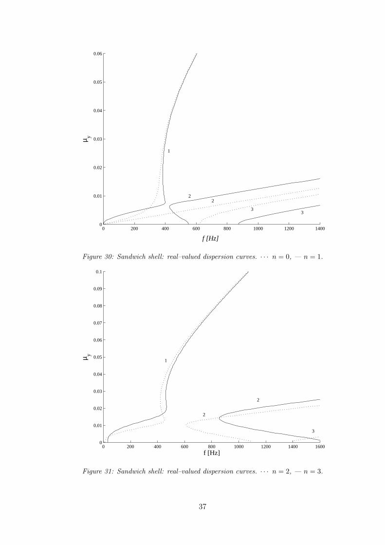
The sandwich shell is made of a bottom skin laminate, a foam core and a top skin laminate.The upper and lower laminae are constituted by 4 orthotropic sheets of glass/epoxy. Eachskin has a lay–up of [+45/-45/-45/+45] and a total thickness of 4 mm. The core is a 10 mmpolymethacrylamide ROHACELL foam with 110WF of density. The different layers and thematerial properties are shown in Figure 29. The nondimensional thickness is h = 0.018.Real–valued dispersion curves are shown in Figures 30–31 for the circumferential modes n =0, 1, 2 and 3. The ring frequency can be considered as the first transition frequency for the thincylinder and it may be evaluated as the frequency at which the third wave starts propagating.Herein, since for n = 0 the branch 3 cuts-on at 617Hz, this frequency value is taken as the ringfrequency for the sandwich cylindrical shell. The minimum cut-off frequencies for branches 2and 1 are 550.3Hz and 11.5Hz respectively. As expected the wave behaviour below the ringfrequency is very complex and cannot be described simply in terms of torsional, extensionaland flexural waves alone. It can be seen in Figure 30 that the n = 1 branches 1 and 2 exhibitmore than one possible value of µy for the same value of frequency. For the n = 1 branch 1,three values of µy can be identified by the same frequency when 384Hz< f < 399Hz, Figure30. The lower and the higher value correspond to waves with positive group velocity in the ydirection while the middle value corresponds to a wave which has a negative group velocity inthe y direction. For n = 1 branch 2, in the frequency range 428Hz< f < 550Hz, two values ofµy correspond to two different waves travelling in opposite y direction, Figure 30. In particular,the wave associated with the lower value of µy has a negative group velocity in the y direction.Similar conclusions can be drawn for the dispersion curves in Figure 31. For n = 0 and n = 1only waves 1 and 2 propagate below the ring frequency. For n = 2, wave 2 still propagates forfrequencies close to the ring frequency, while for n = 3 only wave 1 propagates below the ringfrequency.

36

0 200 400 600 800 1000 1200 14000

0.01

0.02

0.03

0.04

0.05

0.06

f [Hz]

µ y

1

2 2

3 3

Figure 30: Sandwich shell: real–valued dispersion curves. · · · n = 0, — n = 1.

0 200 400 600 800 1000 1200 1400 16000

0.01

0.02

0.03

0.04

0.05

0.06

0.07

0.08

0.09

0.1

f [Hz]

µ y

1

2

2

3

Figure 31: Sandwich shell: real–valued dispersion curves. · · · n = 2, — n = 3.

37

−0.08 −0.06 −0.04 −0.02 0 0.02 0.04 0.06 0.08−0.06

−0.04

−0.02

0

0.02

0.04

0.06

µx

µ y1

1

2

2

Figure 32: Sandwich shell: dispersion curves in the (µx, µy) plane. — f = 200Hz, · · · f = 500Hz.

−0.1 −0.05 0 0.05 0.1−0.1

−0.08

−0.06

−0.04

−0.02

0

0.02

0.04

0.06

0.08

0.1

µx

µ y

1

2

3

Figure 33: Sandwich shell: dispersion curves in the (µx, µy) plane for f = 800Hz.

38

Low frequency dispersion curves in the (µx, µy) plane are shown in Figures 32–34 for differentvalues of frequency. It can be seen in Figures 32–34 that there exists regions for branch 2in which distinct values of µx correspond to the same value of µy and distinct values of µy

correspond to the same value of µx. For every one of these points, considerations about theenergy flow can be made analogous to that for the isotropic shell. A comparison between thedispersion curves 32–34 and results obtained by Heron using an analytical approach for a similarcurved panel [40] has shown that the dispersion curves are almost identical in shape.

−0.15 −0.1 −0.05 0 0.05 0.1 0.15

−0.1

−0.05

0

0.05

0.1

0.15

µx

µ y

1

2

3

Figure 34: Sandwich shell: dispersion curves in the (µx, µy) plane for f = 1500Hz.

39

5. Concluding remarks

A method for the numerical prediction of the wave characteristics of 2–dimensional structuresusing standard FEM has been discussed. With this method only one rectangular FE with 4nodes is used to describe the dynamics of the system reducing drastically the cost of calculations.The mass and stiffness matrices of the element are found using conventional FE approaches andthus the output of commercial FE package can be used. The mass and stiffness matrices aresubsequently post–processed using periodicity conditions in order to formulate an eigenprob-lem whose eigenvalues and eigenvectors describe the wave propagation characteristics. Thiseigenproblem is the kernel of the method and can be cast in a form to provide the propagatingfrequencies and the waveforms for given values of the propagation constants, or to evaluate thepropagation constants for given values of the frequency. The latter approach predicts complexwavenumbers and therefore can be extended to the analysis of general cases, for example inpresence of energy dissipation.The method has been applied to several examples. The first example concerns the out–of–plane vibration of an isotropic plate. Using this example some considerations about generalfeatures of the method have been drawn. It has been found that the frequency of propagationis a periodic function of the real propagation constants. It has also been observed that thewaves propagate across the structure only within some propagating bands. The number ofthese bands, and therefore the number of frequencies and waveforms, depend on the numberof the nodal DOFs chosen for the element. Further, it has been shown that some of themrepresent the behaviour of the continuous model, while others are numerical solutions due tothe discretisation of the system. A sensitivity analysis has been carried out in order to evaluatethe set of solutions which correspond to the continuous structure. The second example dealswith an orthotropic plate made of Glass/Epoxy composite material. In the last part cylindricalshells have been considered. In particular an isotropic and a sandwich curved shell have beenanalysed. These last two cases have been studied by postprocessing an ANSYS FE model.Since the shell elements obtained from ANSYS are flat shell elements, the matrices of a singleelement are manipulated to model the desired curvature for the corresponding curved shell. Theexample of the sandwich cylindrical shell has proved the usefulness of the method for predictingdispersion curves when analytical solutions are not available.The main advantages of the technique can be thus summarised as follows:

• the computational cost becomes independent of the size of the structure since the methodinvolves typically just one finite element to which periodicity conditions are applied;

• the technique is very flexible since standard FE routines can be used and therefore a widerange of structural configurations can be easily analysed;

• finally, the propagation constants for plane harmonic waves can be predicted for differentpropagation directions along the structure.

The method is seen to give accurate predictions when the length of the element is small enoughcompared to the wavelength, that is when the length of the single element is less then 1/6–1/10of the wavelength.Further work should be done to improve the analysis presented in this memorandum. In partic-ular, advances of the post–processing algorithms are needed in order to obtain the complete setof the complex–valued dispersion curves. Future work may also concern the evaluation of the

40

response to external loads such as point forces or random pressure fields. It is also of interestto extend the applicability of the method to non–rectangular finite elements.

41

References

[1] S. Finnveden, “Exact spectral finite element analysis of stationary vibrations in a railwaycar structures”, Acta Acustica, Vol. 2, pp. 461-482, 1994.

[2] L. Gavric, “Computation of propagative waves in free rail using a finite element technique”,Journal of Sound and Vibration, Vol. 184, pp. 531-543, 1995.

[3] U. Orrenius, S. Finnveden, “Calculation of wave propagation in rib-stiffened plate struc-tures”, Journal of Sound and Vibration, Vol. 198, pp. 203-224, 1996.

[4] S. Finnveden, “Spectral finite element analysis of the vibration of straight fluid-filled pipeswith flanges”, Journal of Sound and Vibration, Vol. 199, pp. 125-154, 1997.

[5] P. J. Shorter, “Wave propagation and damping in linear viscoelastic laminates”, Journal ofthe Acoustical Society of America, Vol. 115, pp. 1917-1925, 2004.

[6] J. F. Doyle, “Wave propagation in structures”, Springer-Verlag, 1997.

[7] J. R. Banerjee, “Dynamic stiffness formulation for structural element: a general approach”,Computers Structures, Vol. 63(1), pp. 101-103, 1997.

[8] H. von. Flotow, “Disturbance propagation in structural networks”, Journal of Sound andVibration, Vol. 106, pp. 433-450, 1986.

[9] L. S. Beale, M. L. Accorsi, “Power flow in two- and three-dimensional frame strucutres”,Journal of Sound and Vibration, Vol. 185, pp. 685-702, 1995.

[10] L. Brillouin, “Wave propagation in periodic structures”, Dover Publications, 1953.

[11] D. J. Mead, “Free wave propagation in periodically supported infinite beams”, Journal ofSound and Vibration, Vol. 11(2), pp. 181-197, 1970.

[12] R. M. Orris, M. Petyt “A finite element study of harmonic wave propagation in periodicstructures”, Journal of Sound and Vibration, Vol. 33(2), pp. 223-236, 1974.

[13] D. J. Mead, “wave propagation and natural modes in periodic system: I. mono-coupledsystems”, Journal of Sound and Vibration, Vol. 40(1), pp. 1-18, 1975.

[14] D. J. Mead, “Wave propagation and natural modes in periodic systems: II. Multi-coupledsystems, with and without damping”, Journal of Sound and Vibration, Vol. 40(1), pp.19-39, 1975.

[15] D. J. Mead, “Wave propagation in continuous periodic structures: research contributionsfrom Southampton”, Journal of Sound and Vibration, Vol. 190, pp. 495-524, 1996.

[16] D. Duhamel, B. R. Mace, M. J. Brennan, “Finite element analysis of the vibration ofwaveguides and periodic structures”, Journal of Sound and Vibration, Vol. 294, pp. 205-220, 2006.

[17] B. R. Mace, D. Duhamel, M. J. Brennan, L. Hinke, “Finite element prediction of wavemotion in structural waveguides”, Journal of the Acoustical Society of America, Vol. 117,pp. 2835-2843, 2005.

42

[18] B. R. Mace, D. Duhamel, M. J. Brennan, L. Hinke, “Wavenumber prediction using finite el-ement analysis”, Eleventh International Congress on Sound and Vibration, St. Petersburg,2004.

[19] A. Y. A. Abdel-Rahman, “Matrix analysis of wave propagation in periodic systems”, PhDthesis, University of Southampton, 1979.

[20] R. A. Tapia, “The Kantorovich Theorem for Newton’s Method”, The American Mathemat-ical Monthly, Vol. 78(4), pp. 389-392, 1971.

[21] K. V. Singh, Y. M. Ram, “Transcendental eigenvalue problem and its applications”, AIAAJournal, Vol.40(7), pp. 1402-1407, 2002.

[22] W. H. Yang, “A method for eigenvalues of sparse λ-matrices”, International Journal forNumerical Methods in Engineering, Vol.19(6), pp. 943-948, 1983.

[23] M. J. D. Powell, “A Fortran Subroutine for Solving Systems of Nonlinear Algebraic Equa-tions”, Numerical Methods for Nonlinear Algebraic Equations, P. Rabinowitz, Ch.7, 1970.

[24] L. E. Bateson, M. A. Kelamanson, C. Knudsen “Solution of a transcendental eigenvalueproblem via interval analysis”, Computers and Mathematics with Applications, Vol.38, pp.133-142, 1999.

[25] R. E. Moore, “Interval Analysis”, Prentice-Hall, Englewood Cliff, N. J., 1966.

[26] E. Kreyszig, “Advanced Engineering Mathematics”, John Whiley Son, 1999.

[27] C. F. Gerald, “Applied Numerical Analysis”, Addison-Wesley, 1999.

[28] M. Petyt, “Introduction to finite element vibration analysis” Cambridge University Press,New York, USA, 1990.

[29] S. P. Timoshenko, S. Woinowsky-Krieger, “Theory of plates and shells” McGraw-Hill, 1959.

[30] A. W. Leissa, Vibration of Shells, NASA SP-288, 1973.

[31] D. C. Gazis, “Three-dimensional investigation of the propagation waves in hollow circularcylinders. I. Analytical foundation”, The Journal of the Acoustical Society of America, Vol.31(5), pp. 568-573, 1959.

[32] D. C. Gazis, “Three-dimensional investigation of the propagation pf waves in hollow circularcylinders. II. Numerical Results”, The Journal of the Acoustical Society of America, Vol.31(5), pp. 573-578, 1959.

[33] R. Kumar, R. W. B. Stephens, “Dispersion of flexural waves in circular cylindrical shells”,Proceedings of the Royal Society of London, pp. 283-297, 1972.

[34] C. R. Fuller, “The effects of wall discontinuities on the propagation of flexural waves incylindrical shells”, Journal of Sound and Vibration, Vol. 75, pp. 207-228, 1981.

[35] C. R. Fuller, F. J. Fahy, “Characteristics of wave propagation and energy distributions incylindrical elastic shells filled with fluid”, Journal of Sound and Vibration, Vol. 81, pp.501-518, 1982.

43

[36] R. S. Langley, “Wave motion and energy flow in cylindrical shells”, Journal of Sound andVibration, Vol. 169, pp. 29-42, 1994.

[37] R. S. Langley, “The modal density and mode count of thin cylinders and curved panels”,Journal of Sound and Vibration, Vol. 169, pp. 43-53, 1994.

[38] V. V. Tyutekin, “Helical waves of an elastic cylindrical shell”, Acoustical Physics, Vol.50(3), pp. 273-277, 2004.

[39] V. V. Tyutekin, “Circumferential and helical normal waves of a cylindrical waveguide:helical waves in a free space”, Acoustical Physics, Vol. 52(4), pp. 471-476, 2006.

[40] K. Heron, “Curved laminates and sandwich panels within predictive SEA”, Proceedings ofthe Second International AutoSEA Users Conference, Troy, Michigan, USA, 2002.

44