Embed Size (px)
Citation preview

R0112 July 2006
Client: Civil Engineering Division of Rijkswaterstraat
Modelling uncertainty in inspections of highway bridges in the Netherlands
using Hidden Markov Models
Author: Magdalena Sztul
Delft University of Technology


Members of the committee:
Chairperson of the Committee: Prof. Dr. Ir. Jan M. van Noortwijk
Committee:
Prof. Dr. Ir. Jan M. van Noortwijk Delft University of Technology, Faculty of Electrical
Engineering, Mathematics and Computer Science
HKV Consultants
Dr. Hans van der Weide Delft University of Technology, Faculty of Electrical
Engineering, Mathematics and Computer Science
Ir. Maarten-Jan Kallen HKV Consultants
Ir. Leo Klatter Civil Engineering Division of Rijkswaterstaat
Prof. Dr hab. Jolanta Misiewicz University of Zielona Góra, Poland
Delft, the Netherlands, 2006


Acknowledgments
I am very grateful to Maarten-Jan Kallen for the introduction into the subject and the
entire help during this work. I am also really thankful to Jan van Noortwijk for the supervision of
my thesis, invaluable advices and his assistance during my research. I would like to thank HKV
Consultants for giving me the opportunity to write the thesis within the company and to gain
useful experience.
Many acknowledgments to the Delft University of Technology, to Roger Cooke and
Dorota Kurowicka and also to Jolanta Misiewicz from University of Zielona Góra for giving me
the chance to be here, study and learn life.
I am grateful to my friends: Gosia and Marcin for their friendship and permanent
support. There are no words to express my feelings for you. I will remember this forever!
Also many thanks to Sandra, Sandro, Veronica, Weronika, Beata, Agnieszka, Patrycja
and all my colleagues for being here together and for every kindness.
I would also like to thank my family and friends, especially the one person who has
supported me all the time...


Abstract
In the Netherlands, the inspections of bridges are carried out periodically and their
results are registered in an electronic database. On the basis of visual inspections, bridges are
rated on a discrete scale ranging from a perfect condition to a very bad condition (failure).
Among others, the inspections supply information about the transitions between the bridges'
conditions. Modelling a bridge deterioration process is an important issue in order to gain better
knowledge about the remaining time to failure. The Markovian approach is in our interest as the
condition of the bridges can be expressed by discrete numbers. However a standard Markov
model requires the states to be known without uncertainty. We believe that the results of
inspections can be prone to a bias due to inspectors' subjectivity. Therefore, we consider a
hidden Markov model. This model describes the deterioration process which is assumed to be
Markov with unknown parameters. The hidden parameters (actual states) must be determined
from the observable parameters (observations from the inspections).
To determine the optimal model parameters, the likelihood function of the data was
derived and the maximum likelihood estimator was used. The research presents different
approaches for determining the inspector errors and their results are compared.


July 2006 Hidden Markov Models
HKV CONSULTANTS R0112 i
Contents
Samenvatting ................................................................................................. 1
1 Introduction ............................................................................................. 5 1.1 Applications of the Hidden Markov Model in the literature .....................................................5 1.2 Bridges in the Netherlands................................................................................................6
1.2.1 Bridge data ........................................................................................................6 1.2.2 Visual inspection of the bridges.............................................................................7 1.2.3 Explanation of the choice for a hidden Markov model ...............................................8
1.3 The goal of the research...................................................................................................9
2 Markov and Hidden Markov Models......................................................... 11 2.1 A brief introduction to Markov Chains............................................................................... 11 2.2 An extension of Markov Chains to the Hidden Markov Model ............................................... 12 2.3 Assumptions ................................................................................................................. 13
3 Specification of misclassification error ................................................... 15 3.1 Finding a proper misclassification matrix .......................................................................... 15 3.2 Binomial distribution for the misclassification parameters ................................................... 17 3.3 The maximum entropy principle ...................................................................................... 18
3.3.1 Lagrange multipliers .......................................................................................... 19 3.3.2 Newton-Raphson method ................................................................................... 20 3.3.3 Binomial distribution with fixed mean .................................................................. 22
3.4 The relative information principle..................................................................................... 24
4 Estimation of model parameters ............................................................. 27 4.1 The Maximum Likelihood Estimation (MLE) ....................................................................... 27 4.2 Likelihood function for different models ............................................................................ 33
4.2.1 Likelihood function for different initial vectors ....................................................... 35
5 Expected actual and observed condition................................................. 37 5.1 The expected actual state: E(X(t))................................................................................... 37 5.2 The expected observation: E(O(t)) .................................................................................. 40 5.3 The probability of the actual state given the observation .................................................... 43
6 First time to reach a failure .................................................................... 49 6.1 Perfect inspections......................................................................................................... 49 6.2 Imperfect inspections..................................................................................................... 50
7 Conclusions ............................................................................................ 63
8 References.............................................................................................A-0
Appendix A: Specific bridges from the data .............................................A-1
Appendix B: Proof of the formula for the likelihood (4-3)........................B-1
Appendix C: The extreme cases from the new data .................................C-1

Hidden Markov Models July 2006
ii R0112 HKV CONSULTANTS
Appendix D: Proof of the recursive formula (6-8), p.51 ...........................D-1
Appendix E: First ‘observation’ time........................................................ E-1

July 2006 Hidden Markov Models
HKV CONSULTANTS R0112 iii
List of tables
Table 1-1: A part of the data.................................................................................................................................7
Table 1-2: Condition rating scheme........................................................................................................................8
Table 3-1: The discrete uniform distribution and its entropy.....................................................................................18
Table 3-2: The MaxEntr distribution and its entropy value .......................................................................................22
Table 3-3: The binomial distribution with fixed mean and its entropy value ................................................................23
Table 3-4: Juxtaposition of the values of the entropy for both distributions ................................................................23
Table 3-5: The relative information of binomial with respect to Max.Entr. distribution ..................................................24
Table 3-6: The relative information of binomial with respect to uniform distribution.....................................................25
Table 3-7: The relative information of Max.Entr with respect to uniform distribution ....................................................25
Table 4-1: The value of the entropy for the optimal binomial model ..........................................................................33
Table 4-2: The values of the log-likelihood functions...............................................................................................34
Table 4-3: The values of the log-likelihood functions...............................................................................................35
Table 4-4: The value of the likelihood for the different initial vector ..........................................................................36
Table 5-1: Probability of an actual state given the observation, t=12 months .............................................................44
Table 5-2: Probability of an actual state given the observation, t=24 months .............................................................45
Table 5-3: Probability of an actual state given the observation, t=36 months .............................................................46
Table 5-4: Probability of an actual state given the observation, t=120 months............................................................47
Table 8-1: Specific structures from the data ........................................................................................................ A-2
Table 8-2: Extreme conditions from the new data................................................................................................. C-2


July 2006 Hidden Markov Models
HKV CONSULTANTS R0112 v
List of figures
Figure 1-1: The amount of particular conditions in the data .......................................................................................8
Figure 3-1: Condition rating for the bridge with index 417, permissible error of one state.............................................16
Figure 3-2: Condition rating for the bridge with index 417, permissible error of two states..........................................16
Figure 4-1: Log-likelihood function with ‘Misclassification matrix 1’, ]1:0[∈p .......................................................29
Figure 4-2: Log-likelihood function with ‘Misclassification matrix 1’, ]035.0:0[∈p ..............................................30
Figure 5-1: The expectation of actual state as a function of age................................................................................38
Figure 5-2: The expectation of an actual state as a function of age ...........................................................................38
Figure 5-3: The expectation of an actual state for the new data................................................................................39
Figure 5-4: The expected observation as a function of age, binomial model................................................................40
Figure 5-5: The expected observation as a function of age, uniform model.................................................................41
Figure 5-6: The expected observation as a function of age, Max.Entr and fixed binomial model .....................................42
Figure 5-7: The expected observation as a function of age, models with misclassification matrices: ‘1’ and ‘2’ .................42
Figure 5-8: Probability of the actual state given the observation, t=12 months ...........................................................44
Figure 5-9: Probability of the actual state given the observation, t=24 months ...........................................................45
Figure 5-10: Probability of the actual state given the observation, t=48 months .........................................................46
Figure 5-11: Probability of the actual state given the observation, t=120 months........................................................47
Figure 6-1: First passage time for a forward process, 05f ......................................................................................50
Figure 6-2: First ‘observation’ time for optimal binomial model, inspections carried out each year, *
05f .........................53
Figure 6-3: First ‘observation’ time for optimal binomial model, inspections carried out each 24 months, *
05f .................54
Figure 6-4: First ‘observation’ time for optimal binomial model, inspections carried out each 36 months, *
05f .................54
Figure 6-5: First ‘observation’ time for optimal binomial model, inspections carried out each 48 months, *
05f ................55
Figure 6-6: First ‘observation’ time for optimal binomial model, inspections carried out each 120 months, *
05f ..............55
Figure 6-7: First time of observation the condition ‘3’ for optimal binomial model, inspections carried out each 12
months, *
03f ............................................................................................................................56
Figure 6-8: First time of observation the condition ‘3’ for optimal binomial model, inspections carried out each 24
months, *
03f ............................................................................................................................57
Figure 6-9: First time of observation the condition ‘3’ for optimal binomial model, inspections carried out each 36
months, *
03f ............................................................................................................................57
Figure 6-10: First time of observation the condition ‘3’ for optimal binomial model, inspections carried out each 48
months, *
03f ............................................................................................................................58
Figure 6-11: First time of observation the condition ‘3’ for optimal binomial model, inspections carried out each 120
months, *
03f ............................................................................................................................58
Figure 6-12: First ‘observation’ time for Max.Entr model, inspections carried out each 12 months, *
05f .........................59
Figure 6-13: First ‘observation’ time for Max.Entr model, inspections carried out each 24 months, *
05f .........................59
Figure 6-14: First ‘observation’ time for Max.Entr model, inspections carried out each 36 months, *
05f .........................60
Figure 6-15: First ‘observation’ time for Max.Entr model, inspections carried out each 48 months, *
05f .........................60
Figure 6-16: First ‘observation’ time for Max.Entr model, inspections carried out each 120 months, *
05f ........................61
Figure 8-1: Average condition for the new data.................................................................................................... C-2
Figure 8-2: First ‘observation’ time, inspections carried out each 12 months, *
05f .....................................................E-1
Figure 8-3: First ‘observation time, inspection carried out each 24 month, *
05f .........................................................E-1
Figure 8-4: First ‘observation’ time, inspection carried out each 36 month, *
05f ........................................................E-2
Figure 8-5: First ‘observation’ time, inspection carried out each 48 month, *
05f ........................................................E-2
Figure 8-6: First ‘observation’ time, inspection carried out each 4800 month, *
05f ....................................................E-3
Figure 8-7: First ‘observation’ time, inspection carried out each 12 month, *
05f ........................................................E-3
Figure 8-8: First ‘observation’ time, inspection carried out each 24 month, *
05f ........................................................E-4
Figure 8-9: First ‘observation’ time, inspection carried out each 36 month, *
05f ........................................................E-4
Figure 8-10: First ‘observation’ time, inspection carried out each 48 month, *
05f ......................................................E-5
Figure 8-11: First ‘observation’ time, inspection carried out each 120 month, *
05f .....................................................E-5


July 2006 Hidden Markov Models
HKV CONSULTANTS R0112 1
Samenvatting
Dit rapport is het resultaat van het afstudeerproject van Magda Sztul, studente
Technische Wiskunde aan de faculteit Elektrotechniek, Wiskunde en Informatica (EWI) van de
Technische Universiteit Delft. Het project is uitgevoerd in de periode van januari tot juli 2006 bij
HKV LIJN IN WATER te Lelystad onder begeleiding van ir. M.J. Kallen en prof. dr. ir. J.M. van
Noortwijk.
Introductie
Bruggen en viaducten die onderdeel uitmaken van de rijkswegen in Nederland worden
beheerd door de Bouwdienst (Rijkswaterstaat, Ministerie van Verkeer en Waterstaat). Om de
kwaliteit van deze belangrijke objecten te waarborgen, worden ze periodiek geïnspecteerd. Dit
zijn visuele inspecties die op een doorlopende basis over het hele netwerk van bruggen en
viaducten worden uitgevoerd. Tijdens de inspecties worden verschillende onderdelen van een
brug nauwkeurig bekeken en kent de inspecteur aan elk onderdeel een toestandsindicator toe.
Er zijn zeven discrete toestanden gedefinieerd en deze zijn weergegeven in Tabel 0-1.
Tabel 0-1: toestandsindicatoren in DISK
Indicator Staat van onderhoud van kunstwerkdeel
0 in prima staat
1 in zeer goede staat
2 in goede staat
3 in redelijke staat
4 in matige staat
5 in slechte staat
6 in zeer slechte staat
De gegevens van elke inspectie worden geregistreerd in het Data Informatie Systeem
Kunstwerken (DISK). Dit systeem is al sinds december 1985 in gebruik en bevat derhalve bijna
20 jaar aan gegevens.
Omdat de interpretatie van de toestanden in Tabel 0-1 kunnen verschillen van persoon
tot persoon, en omdat de interpretatie van de ernst van een schade en de algemene toestand
van een brug ook subjectief zijn, is het mogelijk dat de inspecties onzekerheid (in de vorm van
variabiliteit) toevoegen aan de gegevens. Het algemene doel van het afstudeeronderzoek is om
een model toe te passen op de gegevens, waarin rekening gehouden wordt met de onzekerheid
in de inspecties.
Omdat de veroudering van bruggen gemodelleerd wordt met behulp van Markovketens,
wordt in dit onderzoek gebruik gemaakt van zogenaamde ‘hidden Markov’ modellen. Deze
vormen een uitbreiding van de gewone Markovketens waarin ook de kans op een verkeerde
classificatie door de inspecteurs wordt meegenomen. Er wordt dus aangenomen dat een brug
verouderd volgens een Markovketen en dat de inspecteurs de daadwerkelijke toestand zo goed
Hidden Markov Models July 2006
2 R0112 HKV CONSULTANTS
mogelijk proberen te bepalen. De echte toestand van een brug is in dit model als het ware
‘verborgen’ voor de beheerder.
De vraag van de beheerder, in dit geval de Bouwdienst van Rijkswaterstaat, is of een
dergelijk model geschikt is voor toepassing op de inspectiegegevens van bruggen in Nederland.
Zo ja, dan is de vraag in welke vorm en onder welke aannames dit het geval is. Een bijkomend
doel van het onderzoek is om een gevoel te krijgen van het gebruik van een dergelijk model en
om een indruk te krijgen van de inspanning die nodig is om een dergelijk model te
implementeren.
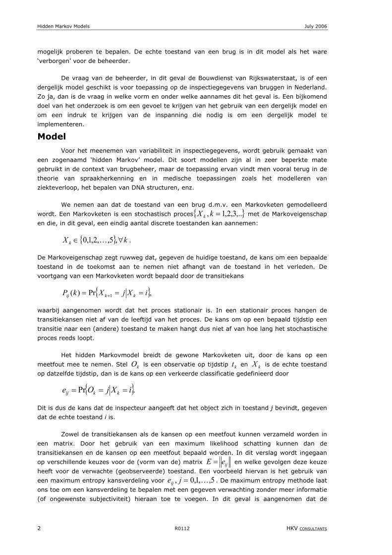
Model
Voor het meenemen van variabiliteit in inspectiegegevens, wordt gebruik gemaakt van
een zogenaamd ‘hidden Markov’ model. Dit soort modellen zijn al in zeer beperkte mate
gebruikt in de context van brugbeheer, maar de toepassing ervan vindt men vooral terug in de
theorie van spraakherkenning en in medische toepassingen zoals het modelleren van
ziekteverloop, het bepalen van DNA structuren, enz.
We nemen aan dat de toestand van een brug d.m.v. een Markovketen gemodelleerd
wordt. Een Markovketen is een stochastisch proces{ },..3,2,1, =kX k met de Markoveigenschap
en die, in dit geval, een eindig aantal discrete toestanden kan aannemen:
{ } kX k ∀∈ ,5,,2,1,0 K .
De Markoveigenschap zegt ruwweg dat, gegeven de huidige toestand, de kans om een bepaalde
toestand in de toekomst aan te nemen niet afhangt van de toestand in het verleden. De
voortgang van een Markovketen wordt bepaald door de transitiekans
{ },Pr)( 1 iXjXkP kkij === +
waarbij aangenomen wordt dat het proces stationair is. In een stationair proces hangen de
transitiekansen niet af van de leeftijd van het proces. De kans om op een bepaald tijdstip een
transitie naar een (andere) toestand te maken hangt dus niet af van hoe lang het stochastische
proces reeds loopt.
Het hidden Markovmodel breidt de gewone Markovketen uit, door de kans op een
meetfout mee te nemen. Stel kO is een observatie op tijdstip kt en kX is de echte toestand
op datzelfde tijdstip, dan is de kans op een verkeerde classificatie gedefinieerd door
{ }.Pr iXjOe kkij ===
Dit is dus de kans dat de inspecteur aangeeft dat het object zich in toestand j bevindt, gegeven
dat de echte toestand i is.
Zowel de transitiekansen als de kansen op een meetfout kunnen verzameld worden in
een matrix. Door het gebruik van een maximum likelihood schatting kunnen dan de
transitiekansen en de kansen op een meetfout bepaald worden. In dit verslag wordt ingegaan
op verschillende keuzes voor de (vorm van de) matrix ijeE = en welke gevolgen deze keuze
heeft voor de verwachte (geobserveerde) toestand. Een voorbeeld hiervan is het gebruik van
een maximum entropy kansverdeling voor 5,,1,0, K=jeij . De maximum entropy methode laat
ons toe om een kansverdeling te bepalen met een gegeven verwachting zonder meer informatie
(of ongewenste subjectiviteit) hieraan toe te voegen. In dit geval is aangenomen dat de

July 2006 Hidden Markov Models
HKV CONSULTANTS R0112 3
inspecteurs naar verwachting de echte toestand correct observeren. De maximum entropy
methode resulteert in een volledig gevulde matrix met kansen op meetfouten, hetgeen wil
zeggen dat er bijv. een kans is dat inspecteurs een toestand 0 aangeven i.p.v. de echte
toestand 5. Het is ook mogelijk om slechts een gedeeltelijk gevulde kansenmatrix te kiezen,
zodat de meetfout bijv. niet meer dan één of twee toestanden kan afwijken. Voor elke keuze
van de E matrix is het mogelijk deze van te voren vast te leggen (bijv. door de keuze voor een
maximum entropy methode) of deze te schatten aan de hand van de inspectiegegevens. In het
eerste geval nemen we een meetfout aan en in het tweede geval proberen we uit de gegevens
op te maken welke de meest waarschijnlijke meetfout is.
Als laatste is ook gekeken naar de tijd van de eerste observatie van de slechtste
toestand (namelijk toestand 5) indien we aannemen dat elk object vanuit de perfecte toestand
0 begint. Deze tijd is onzeker en is vergelijkbaar met de zogenaamde ‘first passage time’ voor
de gewone Markovketen. De tijd van eerste passage door een toestand van een Markovproces is
het tijdstip waarop het stochastische proces de desbetreffende toestand de eerste keer
aanneemt. Deze tijd is uiteraard onzeker vanwege de onzekerheid in het verloop van het proces
zelf. Vanwege de extra onzekerheid in de observaties, is de ‘first observation time’ moeilijker te
bepalen en hangt deze af van de tijd tussen de inspecties.
Resultaten en aanbevelingen
De resultaten van het onderzoek worden toegelicht aan de hand van de volgende
onderzoeksvragen:
1. hoe kan de variabiliteit (of onzekerheid) in de observaties van inspecteurs
meegenomen worden in het verouderingsmodel?
Omdat de veroudering gemodelleerd wordt d.m.v. een Markovketen, is de keuze voor het
gebruik van een zogenaamd ‘hidden Markov’ model een natuurlijke keuze. Deze uitbreiding
laat ons toe een kansverdeling over de meetfout van de toestand aan te nemen. Vanuit een
wiskundig oogpunt is het een elegant model en gedraagt het zich zoals men zou
verwachten. Vanuit een praktisch oogpunt, blijkt het lastig om de onzekerheid in de
observaties duidelijk te scheiden van de onzekerheid in de veroudering. Bovendien hangt
het eindresultaat sterk af van de keuze voor de foutmatrix E.
2. wat is de beste keuze voor de waarde van de parameters in het model?
Door het gebruik van de methode van maximum likelihood schatting, kunnen de parameters
in het model zodanig bepaald worden dat de waarschijnlijkheid dat de gegevens
gegenereerd zouden zijn door het model het hoogst is. We kiezen als het ware de waarde
van de parameters zodanig dat de kans op de gegevens het grootst is.
3. hoe bepalen we de likelihood functie die gebruikt wordt voor het schatten van de
parameters?
Voor de maximum likelihood methode is het noodzakelijk om de likelihood functie uit te
rekenen en deze te maximaliseren. Drie verschillende algoritmes voor het bepalen van de
waarschijnlijkheid van de gegevens worden in hoofdstuk 4 gepresenteerd.
4. hoe bepalen we de verwachting van de toestand als functie van de leeftijd van een
brug?
Het verwachte toestandsverloop is interessante informatie die uit het toegepaste model
voort vloeit. In hoofdstuk 5 wordt deze verwachting voor verschillende E matrices
geanalyseerd en wordt ook gekeken naar het verschil tussen de verwachting van de echte
toestand en de verwachting van de geobserveerde toestand.
5. hoe berekenen we de kans op een echte toestand, gegeven de observatie?

Hidden Markov Models July 2006
4 R0112 HKV CONSULTANTS
Naast het verloop van de verwachte toestand, zijn we ook geïnteresseerd in de echte
toestand van een object gegeven de observatie van een inspecteur. In hoofdstuk 5 wordt
gedemonstreerd hoe deze kans afhangt van de leeftijd van het object.
6. hoe leiden we een formule af voor het berekenen van de eerste tijd tot observatie
van de slechtste toestand en hoe hangt deze onzekere tijd af van de frequentie
van de inspecties?
Het bepalen van de kansverdeling van de tijd tot de eerste observatie van een toestand
heeft veel weg van het bepalen van de kansverdeling van de zogenaamde ‘first passage
time’ voor Markovprocessen. Door het gebruik van extra onzekerheid over de observaties is
de implementatie echter een stuk moeilijker. Hoofdstuk 6 gaat in op twee manieren om
deze kansverdeling te bepalen. Een belangrijk feit is dat deze kansverdeling afhankelijk is
van de frequentie van de inspecties. Een observatie kan immers alleen gemaakt worden
tijdens een inspectie. Het blijkt dat de verwachte tijd tot de eerste observatie van toestand
5 groter wordt naarmate het inspectie interval vergroot wordt. In de praktijk is dit natuurlijk
niet logisch, omdat minder inspecteren zou resulteren in een langere levensduur van het
object. Wiskundig gezien is het model echter correct, omdat er meerdere inspecties nodig
zijn om de laatste toestand te observeren vanwege de meetfout.
De volgende aanbevelingen worden gedaan:
• in dit onderzoek zijn zowel de transitiekansen als de kansen op meetfouten stationair
aangenomen. D.w.z. dat deze onafhankelijk zijn van de leeftijd van het object, of van de
tijd dat ze in een bepaalde toestand verbracht hebben. De aanbeveling is om met name de
kansen op meetfouten tijdsafhankelijk te maken, zodat bijv. de kans op het verkeerd
observeren van de laatste en slechtste toestand steeds kleiner wordt naarmate het object
ouder wordt.
• Het is aanbevolen om de variabiliteit in de observaties van inspecteurs te testen,
bijvoorbeeld d.m.v. een proefopzet waarbij verschillende inspecteurs gevraagd wordt een
bepaald object te classificeren. Interessant zou zijn om na te gaan wat de grootste fout is
die gemaakt wordt door één van de inspecteurs. De informatie uit een dergelijke toets kan
ondersteuning bieden voor het bepalen van de fouten kansmatrix E.
• Het uitrekenen van de likelihood functie is op slechts een enkele manier gedaan, terwijl er
nog tenminste twee andere methoden hiervoor bekend zijn. De robuustheid en de
efficiëntie van deze twee andere methoden zou vergeleken kunnen worden met de in dit
verslag toegepaste methode.
• Aangezien onderhoudsacties uit de gegevens zijn gehaald, houdt het hier gepresenteerde
model geen rekening met onderhoud. Het is een uitdaging om deze wel mee te nemen.
July 2006 Hidden Markov Models
HKV CONSULTANTS R0112 5
1 Introduction
The Netherlands Ministry of Transport, Public Works and Water Management is
responsible for the road network in the country. Because of the fact that bridges are a part of
that, it involves also a need to care about them. The bridge maintenance actions are costly
activities, so the minimization of the costs is of highest interest, together with the need to
ensure the safety for the road users. Since 1985, The Civil Engineering Division (‘Bouwdienst’)
of Rijkswaterstaat, which is a part of the ministry, stores the results from the inspections in
electronic database called ‘DISK’. Among others, it supplies information about the transitions
between the bridges’ conditions, which is the most important information for our current
analysis.
Since structures like bridges deteriorate with time, this process is connected with some
randomness, for instance due to environmental factors or difficulty in the precise prediction of
the traffic intensity. Therefore, the deterioration can best be modelled using stochastic
processes. One of such processes is a Markov chain. Markovian models are widely applicable in
describing dynamic processes. However, the standard Markovian processes are based on the
assumption that the actual state of the system is known without uncertainty. Since the
inspections of bridges are carried out visually, it is important to realise that they do not yield
perfect estimates of the real conditions. The estimates can be prone to a bias due to inspectors’
subjectivity. Therefore, a modification of the Markov process is necessary in order to take into
consideration this possible error due to the inspectors’ subjectivity.
The thesis presents the idea of applying the Hidden Markov Model to the bridge
inspections in the Netherlands. This model allows considering the results of inspections as
observations that hide the information about the real states. Hence, it is suitable for our
analysis. The standard Markov process is described by the transition probabilities between all
possible states which create the transition matrix. The extension of the Markov model to the
Hidden Markov model adds additional parameters to the problem, namely all the probabilities
that describe an error between the real state and the given assessment of the state
(observation).
The work is conducted under the supervision of Delft University of Technology and HKV
Consultants, and with the cooperation of The Civil Engineering Division of Rijkswaterstraat. The
Civil Engineering Division provided the data and HKV Consultants the precious advices related
with the research direction.
1.1 Applications of the Hidden Markov Model in the literature
Neither the theory of Hidden Markov models (HMM’s) nor their application is new. They
are widely used in many science disciplines like for instance medicine, computer science and
engineering. Hidden Markov Models were first described by Leonard E. Baum in the late 1960s
in the series of statistical papers. One of their first applications was speech recognition in the
mid-1970s. Later on, in the 1980s they start to be omnipresent in many areas, for instance in
the bioinformatics field.
An example of the application of the HMM’s in speech recognition is presented for in [8].
Real-word processes produce observable outcomes called signals. The signal can be often
corrupted from other signal sources. Thanks to the HMM, it is possible to optimally remove the

Hidden Markov Models July 2006
6 R0112 HKV CONSULTANTS
noise from the system. Also, the HMMs provide necessary statistical characteristics of such
signals.
Medicine is using HMM in areas as: genome [11], [12], or pneumology [13] and many
others. However, the continuous HMM are mostly more suitable for those cases.
Exemplary application of the HMM for disease progression was presented by Jackson,
[1]. An early detection of a disease has essential influence on the successive treatment.
Therefore, systematic screening of a population can result in a meaningful reduction of the
mortality from a disease. However the screening process can often be prone to a bias. Then the
actual Markov disease process is not observed directly, but it is hidden inside the realizations.
The diagnosis error is then measured by the misclassification probabilities, i.e. the probabilities
of the screening results given the true states.
The application of the HMM is also not new in bridge management policy. The model is
referred as partially observable Markov decision processes in many sources, like in [16] and
[15]. In the last mentioned document, an error resulting from the uncertainty of measurements
and forecasting in assessments of the highway pavement’s conditions is considered, and the
methodology for maintenance activity selection is derived. The model includes the maintenance
actions after each inspection (which is assumed to be carried out at the beginning of every
year). Therefore, it complicates the regular Hidden Markov Model to a higher extent. It is
assumed that a decision maker observes outputs from the measurements. Those outputs are
related to the actual condition of the system only probabilistically, hence they are not known
with certainty. At the beginning of the planning horizon, the decision maker can evaluate
maintenance policies for the whole horizon. He or she knows at this moment all the history of
the measured states up to this time and the history of all the decisions made up to the previous
action. However, as the uncertainty is introduced to the system, it affects the choice of the
action since a measurement error can lead to the wrong activity. In the aftermath of this wrong
decision the total lifecycle costs could be higher if the correct decision required less costs.
1.2 Bridges in the Netherlands
In the Netherlands, the road network is highly developed. It is easy to see with the
naked eye that good quality roads can lead drivers to every place. However, a lot of the roads
are situated on concrete viaducts and bridges. It is sometimes the only choice to avoid
obstacles like other roads, railways or rivers. The term ‘bridge’ refers mostly to the structure
built over the ‘wet’ obstruction while ‘viaduct’ is called every structure above ‘dry’ obstacles like
highways and railways. In this work both kind of concrete structures are considered, but to
shorten the notation one common name ‘bridge’ will be used further on.
Most of the concrete bridges in the country are getting old, as they are about 40 years
or even more, and soon they will require serious renovation. Such structures can endanger
peoples’ safety, if they are not treated with proper attention. They must be inspected regularly
and a maintenance action should be initiated as soon as a condition of a bridge exceeds the
failure level. For this reason, estimation of the deterioration rate and the failure time, as precise
as possible, is of great interest.
1.2.1 Bridge data
In the Netherlands, the information about the bridges is registered in the electronic
database called ‘DISK’. The database is a huge source of information, not only about the current
July 2006 Hidden Markov Models
HKV CONSULTANTS R0112 7
conditions but also about the location of the bridges, their age, history of inspections, etc. For
this research we do not need the whole database, which has a really complicated structure. We
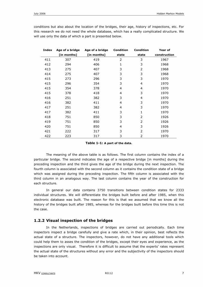
will use only the data of which a part is presented below.
Index Age of a bridge
[in months]
Age of a bridge
[in months]
Condition
state
Condition
state
Year of
construction
411 307 419 2 3 1967
412 294 406 1 3 1968
413 275 407 3 2 1968
414 275 407 3 3 1968
415 273 296 3 3 1970
415 296 354 3 4 1970
415 354 378 4 4 1970
415 378 418 4 3 1970
416 251 382 3 4 1970
416 382 411 4 3 1970
417 251 382 4 3 1970
417 382 411 3 1 1970
418 751 850 3 2 1926
419 751 850 3 2 1926
420 751 850 4 3 1926
421 222 317 3 2 1970
422 223 317 3 2 1970
Table 1-1: A part of the data.
The meaning of the above table is as follows. The first column contains the index of a
particular bridge. The second indicates the age of a respective bridge [in months] during the
preceding inspection and the third gives the age of the bridge during the next inspection. The
fourth column is associated with the second column as it contains the condition state of a bridge
which was assigned during the preceding inspection. The fifth column is associated with the
third column in an analogous way. The last column contains the year of the construction for
each structure.
In general our data contains 3750 transitions between condition states for 2333
individual structures. We will differentiate the bridges built before and after 1985, when this
electronic database was built. The reason for this is that we assumed that we know all the
history of the bridges built after 1985, whereas for the bridges built before this time this is not
the case.
1.2.2 Visual inspection of the bridges
In the Netherlands, inspections of bridges are carried out periodically. Each time
inspectors inspect a bridge carefully and give a rate which, in their opinion, best reflects the
actual state of a structure. The inspectors, however, do not have any additional tools which
could help them to asses the condition of the bridges, except their eyes and experience, as the
inspections are only visual. Therefore it is difficult to assume that the experts’ rates represent
the actual state of the structures without any error and the subjectivity of the inspectors should
be taken into account.

Hidden Markov Models July 2006
8 R0112 HKV CONSULTANTS
Each time when an expert rates a bridge he or she assigns a number to it from
a discrete scale from 0 to 6 where ‘0’ indicates a perfect condition and ‘6’ means that it is in
an extremely bad condition (failure). The table with a description of all the possible conditions is
presented below.
Table 1-2: Condition rating scheme
One remark need to be made here. As the conditions ‘5’ and ‘6’ occur rarely in the data,
we decided to merge these two states together. So in fact we will be working with a discrete
scale of range 6: from 0 to 5.
Figure 1-1 presents the amount of particular conditions in the data (with conditions ‘5’
and ‘6’ together):
Figure 1-1: The amount of particular conditions in the data
1.2.3 Explanation of the choice for a hidden Markov model
The deterioration model used in this analysis is a hidden Markov model. This model was
chosen because the condition of the bridges can be described with the help of a discrete scale
from 0 to 5. Furthermore we use a hidden Markov, not simply a Markov process, since we want
to take into consideration the subjectivity of the inspectors. So we treat the observed condition
states of the bridges not as actual states but rather as observations that can contain some bias.
condition description
0
1
2
3
4
5
6
Perfect
Very good
Good
Reasonable
Mediocre
Bad
Very bad

July 2006 Hidden Markov Models
HKV CONSULTANTS R0112 9
Therefore the observations hide the real state from us and add extra parameters to the Markov
model, namely the probabilities of errors resulting from the experts’ subjectivity.
Another important property of the Markov model, which is useful to us, is that the future
prediction of the state depends only on the present state and the history of the process is not
important. This means that the model has the memoryless property. To predict the deterioration
process of a bridge only the information about the current condition is of interest.
1.3 The goal of the research
The goal of the research is to create a Hidden Markov deterioration process for the
bridges in the Netherlands. The first step in order to do that is to determine the shape of the
matrices with the model parameters, i.e. the transition probability matrix as well as the matrix
with parameters describing the errors between the observations and the actual states (called
misclassification matrix). Later on, for estimating the unknown parameters, the likelihood
function must be derived, which take both kinds of parameters into account. Finally, with the
estimated parameters, some analysis will be carried out in order to gain knowledge about the
expected lifetime of the bridges and how this expectation varies from that obtained without
taking the inspectors’ ‘subjectiveness’ into consideration. We are also interested in finding out
how the intensity of the inspections influences this expectation. Therefore we present the idea
of the time of first passing to a certain actual condition state (first passage time) and its
extension to the time of first observing a certain state (first ‘observation’ time) for different
inspection intervals.
The main questions that are posed in this thesis are:
1. How to introduce the uncertainty resulting from the experts’ subjectivity into the
deterioration model?
2. What is the best choice for the parameters which describe the uncertainty in the
deterioration model?
3. How to derive a statistical function of parameters (likelihood function) that provides
us a tool for finding the parameters that fit the data well?
4. How to determine the expectation of the condition as a function of age?
5. How to calculate and illustrate the probability that a bridge is in an actual state
given inspectors’ ratings?
6. How to derive the recursive formula for the probability density function of the first
‘observation’ time? Furthermore, how this density function changes as the
‘frequency’ of the inspections is changing?
The report is organized as follows:
Chapter 2 presents the theory about the Markov chains and their extension to the
Hidden Markov Models. The necessary notation is introduced and also a way of choosing the
model parameters is described. At the end of this chapter, the assumptions which are needed
for the whole document are presented.

Hidden Markov Models July 2006
10 R0112 HKV CONSULTANTS
In chapter 3, the entropy principle and the relative information are presented in order to
obtain a distribution for the misclassification error which does not add any additional
information other than the expectation of the observation.
Chapter 4 contains the method of estimating the parameters of the deterioration model,
which is the maximum likelihood method. We use this method to maximize the likelihood
function and we obtain the optimal parameters for our model.
Chapter 5 presents the results of calculating the expectation of the actual state and the
observed condition as a function of a bridge age. Also, the probability of the actual state given
the observation is calculated and the results are visualised by use of a ‘bar’ plot.
Chapter 6 demonstrates the idea of the first passage time and its extension to the first
‘observation’ time, which is simply the mean time to observe the worst condition. The analysis
takes into account the ‘frequency’ of the inspections and indicates how this intensity influences
the mean time to failure.
The last chapter 7 is a summary of the analysis and gives recommendations for future
research.
July 2006 Hidden Markov Models
HKV CONSULTANTS R0112 11
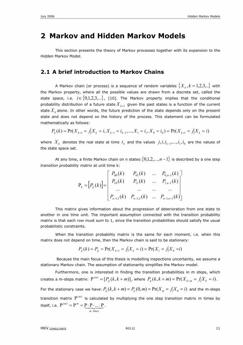
2 Markov and Hidden Markov Models
This section presents the theory of Markov processes together with its expansion to the
Hidden Markov Model.
2.1 A brief introduction to Markov Chains
A Markov chain (or process) is a sequence of random variables { },..3,2,1, =kX k with
the Markov property, where all the possible values are drawn from a discrete set, called the
state space, i.e. { },...3,2,1,0∈i , [10]. The Markov property implies that the conditional
probability distribution of a future state 1+kX given the past states is a function of the current
state kX alone. In other words, the future prediction of the state depends only on the present
state and does not depend on the history of the process. This statement can be formulated
mathematically as follows:
)Pr(),,...,,Pr()( 10011111 iXjXiXiXiXiXjXkP kkkkkkij ========= +−−+
where kX denotes the real state at time kt and the values 011 ,,...,,, iiiij k− are the values of
the state space set.
At any time, a finite Markov chain on n states:{ }1,...,2,1,0 −n is described by a one step
transition probability matrix at unit time k:
[ ]
==Ρ
−−−−
−
−
)(...)()(............
)(...)()()(...)()(
)(
1,12,11,1
1,11110
1,00100
kPkPkP
kPkPkPkPkPkP
kP
nnnn
n
n
ijk
This matrix gives information about the progression of deterioration from one state to
another in one time unit. The important assumption connected with the transition probability
matrix is that each row must sum to 1, since the transition probabilities should satisfy the usual
probabilistic constraints.
When the transition probability matrix is the same for each moment, i.e. when this
matrix does not depend on time, then the Markov chain is said to be stationary:
)Pr()Pr()( 011 iXjXiXjXPkP kkijij ======= +
Because the main focus of this thesis is modelling inspections uncertainty, we assume a
stationary Markov chain. The assumption of stationarity simplifies the Markov model.
Furthermore, one is interested in finding the transition probabilities in m steps, which
creates a m-steps matrix: )],([)( mkkPijm +=Ρ , where )Pr(),( iXjXmkkP kmkij ===+ + .
For the stationary case we have: )Pr(),0(),( 0 iXjXmPmkkP mijij ====+ and the m-steps
transition matrix )(mΡ is calculated by multiplying the one step transition matrix m times by
itself, i.e. 43421timesm
mm Ρ⋅⋅Ρ⋅Ρ=Ρ=Ρ ...)( .
Hidden Markov Models July 2006
12 R0112 HKV CONSULTANTS
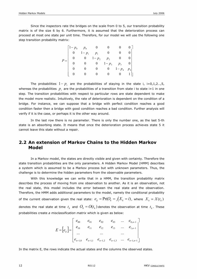
Since the inspectors rate the bridges on the scale from 0 to 5, our transition probability
matrix is of the size 6 by 6. Furthermore, it is assumed that the deterioration process can
proceed at most one state per unit time. Therefore, for our model we will use the following one
step transition probability matrix:
−−
−−
−
=
10000010000
01000001000001000001
44
33
22
11
00
pppp
pppp
pp
P
The probabilities ip−1 are the probabilities of staying in the state i, i=0,1,2…,5,
whereas the probabilities ip are the probabilities of a transition from state i to state i+1 in one
step. The transition probabilities with respect to particular rows are state dependent to make
the model more realistic. Intuitively, the rate of deterioration is dependent on the condition of a
bridge. For instance, we can suppose that a bridge with perfect condition reaches a good
condition faster then a bridge with good condition reaches a bad condition. Further analysis will
verify if it is the case, or perhaps it is the other way around.
In the last row there is no parameter. There is only the number one, as the last 5-th
state is an absorbing state. It means that once the deterioration process achieves state 5 it
cannot leave this state without a repair.
2.2 An extension of Markov Chains to the Hidden Markov Model
In a Markov model, the states are directly visible and given with certainty. Therefore the
state transition probabilities are the only parameters. A Hidden Markov Model (HMM) describes
a system which is assumed to be a Markov process but with unknown parameters. Thus, the
challenge is to determine the hidden parameters from the observable parameters.
With this knowledge we can write that in a HMM, the transition probability matrix
describes the process of moving from one observation to another. As it is an observation, not
the real state, this model includes the error between the real state and the observation.
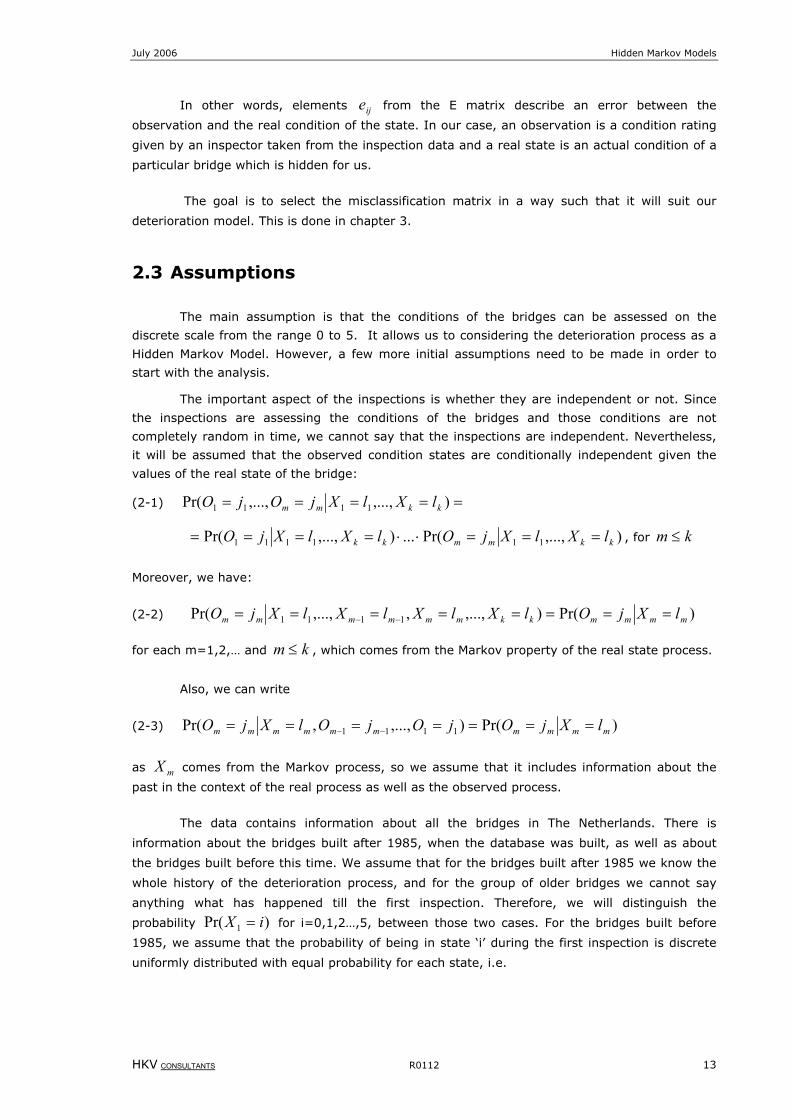
Therefore, the HMM adds additional parameters to the model, namely the conditional probability
of the current observation given the real state: )Pr( iXjOe kkij === , where )( kk tXX =
denotes the real state at time kt and )( kk tOO = denotes the observation at time kt . These
probabilities create a misclassification matrix which is given as below:
[ ]
==
−−−−−−
−
−
1,13,12,11,10,1
1,113121110
1,003020100
...
.........
...
...
nnnnnn
n
n
ij
eeeee
eeeeeeeeee
eE
In the matrix E, the rows indicate the actual states and the columns the observed states.
July 2006 Hidden Markov Models
HKV CONSULTANTS R0112 13
In other words, elements ije from the E matrix describe an error between the
observation and the real condition of the state. In our case, an observation is a condition rating
given by an inspector taken from the inspection data and a real state is an actual condition of a
particular bridge which is hidden for us.
The goal is to select the misclassification matrix in a way such that it will suit our
deterioration model. This is done in chapter 3.
2.3 Assumptions
The main assumption is that the conditions of the bridges can be assessed on the
discrete scale from the range 0 to 5. It allows us to considering the deterioration process as a
Hidden Markov Model. However, a few more initial assumptions need to be made in order to
start with the analysis.
The important aspect of the inspections is whether they are independent or not. Since
the inspections are assessing the conditions of the bridges and those conditions are not
completely random in time, we cannot say that the inspections are independent. Nevertheless,
it will be assumed that the observed condition states are conditionally independent given the
values of the real state of the bridge:
(2-1) ===== ),...,,...,Pr( 1111 kkmm lXlXjOjO
),...,Pr(...),...,Pr( 111111 kkmmkk lXlXjOlXlXjO ===⋅⋅==== , for km ≤
Moreover, we have:
(2-2) )Pr(),...,,,...,Pr( 1111 mmmmkkmmmmmm lXjOlXlXlXlXjO ======== −−
for each m=1,2,… and km ≤ , which comes from the Markov property of the real state process.
Also, we can write
(2-3) )Pr(),...,,Pr( 1111 mmmmmmmmmm lXjOjOjOlXjO ======= −−
as mX comes from the Markov process, so we assume that it includes information about the
past in the context of the real process as well as the observed process.
The data contains information about all the bridges in The Netherlands. There is
information about the bridges built after 1985, when the database was built, as well as about
the bridges built before this time. We assume that for the bridges built after 1985 we know the
whole history of the deterioration process, and for the group of older bridges we cannot say
anything what has happened till the first inspection. Therefore, we will distinguish the
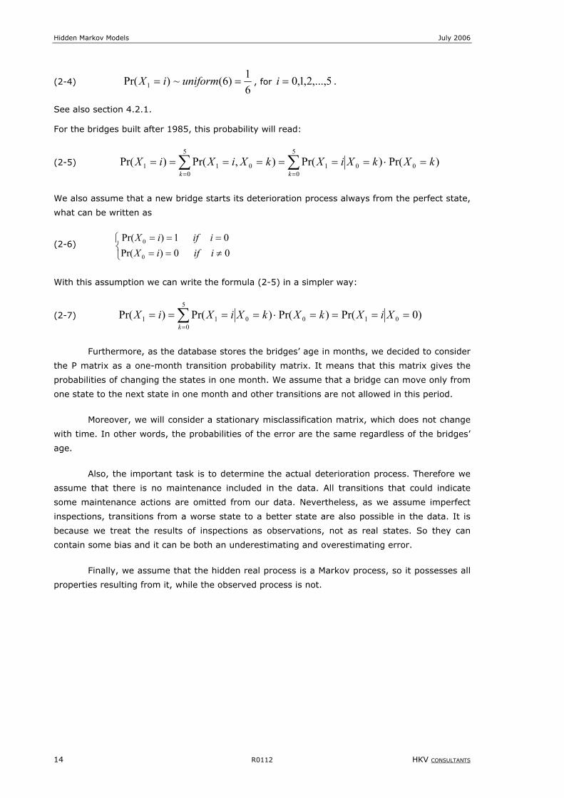
probability )Pr( 1 iX = for i=0,1,2…,5, between those two cases. For the bridges built before
1985, we assume that the probability of being in state ‘i’ during the first inspection is discrete
uniformly distributed with equal probability for each state, i.e.
Hidden Markov Models July 2006
14 R0112 HKV CONSULTANTS
(2-4) 61)6(~)Pr( 1 == uniformiX , for 5,...,2,1,0=i .
See also section 4.2.1.
For the bridges built after 1985, this probability will read:
(2-5) )Pr()Pr(),Pr()Pr( 0
5
001
5
0011 kXkXiXkXiXiX
kk=⋅======= ∑∑
==
We also assume that a new bridge starts its deterioration process always from the perfect state,
what can be written as
(2-6)
≠=====
00)Pr(01)Pr(
0
0
iifiXiifiX
With this assumption we can write the formula (2-5) in a simpler way:
(2-7) )0Pr()Pr()Pr()Pr( 010
5
0011 ====⋅==== ∑
=
XiXkXkXiXiXk
Furthermore, as the database stores the bridges’ age in months, we decided to consider
the P matrix as a one-month transition probability matrix. It means that this matrix gives the
probabilities of changing the states in one month. We assume that a bridge can move only from
one state to the next state in one month and other transitions are not allowed in this period.
Moreover, we will consider a stationary misclassification matrix, which does not change
with time. In other words, the probabilities of the error are the same regardless of the bridges’
age.
Also, the important task is to determine the actual deterioration process. Therefore we
assume that there is no maintenance included in the data. All transitions that could indicate
some maintenance actions are omitted from our data. Nevertheless, as we assume imperfect
inspections, transitions from a worse state to a better state are also possible in the data. It is
because we treat the results of inspections as observations, not as real states. So they can
contain some bias and it can be both an underestimating and overestimating error.
Finally, we assume that the hidden real process is a Markov process, so it possesses all
properties resulting from it, while the observed process is not.
July 2006 Hidden Markov Models
HKV CONSULTANTS R0112 15
3 Specification of misclassification error
In this chapter we will determine a proper form for the misclassification matrix. In other
words, we will determine how wide the possible error resulting from experts’ subjectivity should
be. Next, we will model the misclassification matrix by a few discrete distributions, namely some
discrete distributions with restricted uncertainty bounds (partially filled misclassification matrix),
a binomial distribution, a distribution following from the maximum-entropy method given a fixed
mean and a binomial distribution with fixed mean.
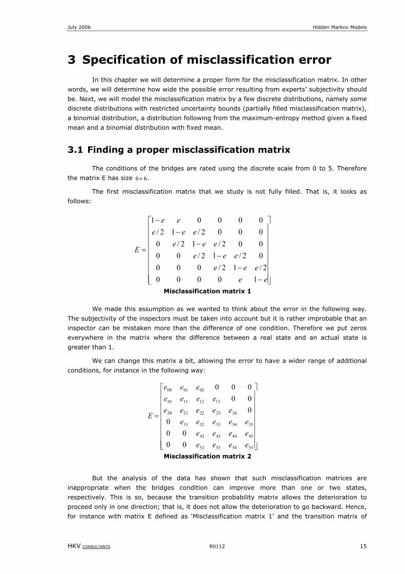
3.1 Finding a proper misclassification matrix
The conditions of the bridges are rated using the discrete scale from 0 to 5. Therefore
the matrix E has size 66× .
The first misclassification matrix that we study is not fully filled. That is, it looks as
follows:
−−
−−
−−
=
eeeee
eeeeee
eeeee
E
100002/12/000
02/12/00002/12/00002/12/00001
Misclassification matrix 1
We made this assumption as we wanted to think about the error in the following way.
The subjectivity of the inspectors must be taken into account but it is rather improbable that an
inspector can be mistaken more than the difference of one condition. Therefore we put zeros
everywhere in the matrix where the difference between a real state and an actual state is
greater than 1.
We can change this matrix a bit, allowing the error to have a wider range of additional
conditions, for instance in the following way:
=
55545352
45444342
3534333231
2423222120
13121110
020100
0000
0000000
eeeeeeeeeeeee
eeeeeeeee
eee
E
Misclassification matrix 2
But the analysis of the data has shown that such misclassification matrices are
inappropriate when the bridges condition can improve more than one or two states,
respectively. This is so, because the transition probability matrix allows the deterioration to
proceed only in one direction; that is, it does not allow the deterioration to go backward. Hence,
for instance with matrix E defined as ‘Misclassification matrix 1’ and the transition matrix of
Hidden Markov Models July 2006
16 R0112 HKV CONSULTANTS
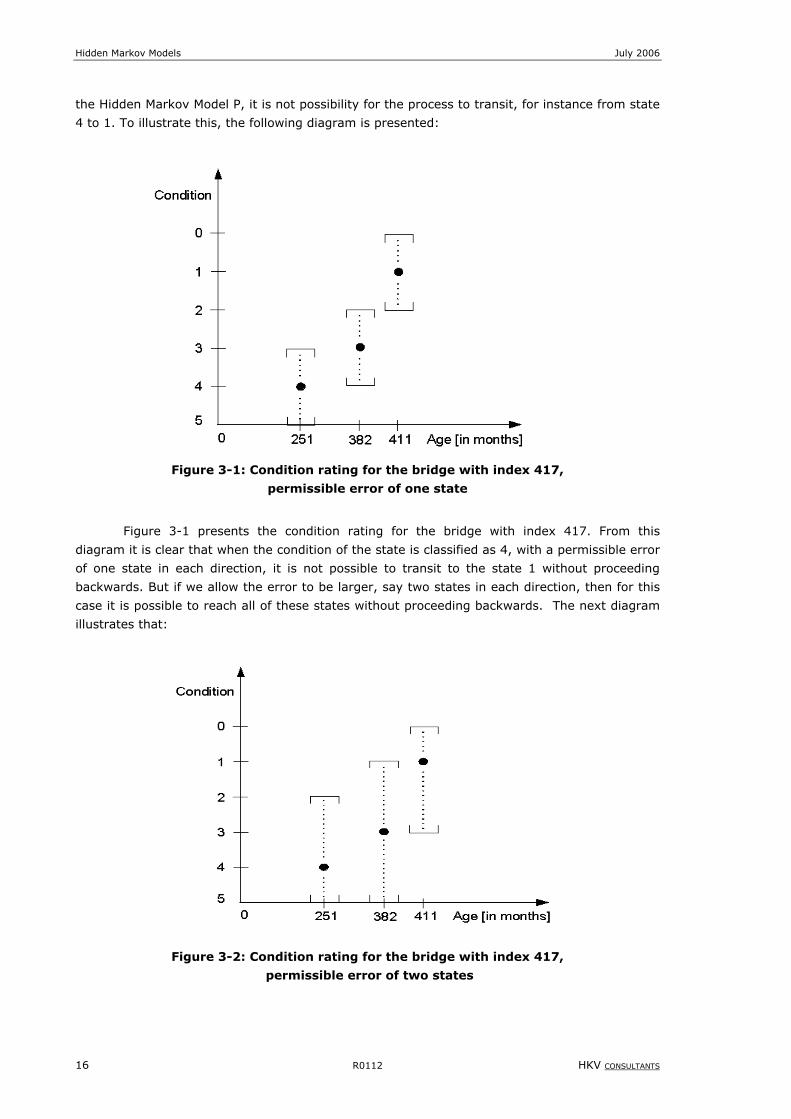
the Hidden Markov Model P, it is not possibility for the process to transit, for instance from state
4 to 1. To illustrate this, the following diagram is presented:
Figure 3-1: Condition rating for the bridge with index 417,
permissible error of one state
Figure 3-1 presents the condition rating for the bridge with index 417. From this
diagram it is clear that when the condition of the state is classified as 4, with a permissible error
of one state in each direction, it is not possible to transit to the state 1 without proceeding
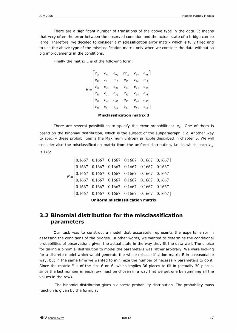
backwards. But if we allow the error to be larger, say two states in each direction, then for this
case it is possible to reach all of these states without proceeding backwards. The next diagram
illustrates that:
Figure 3-2: Condition rating for the bridge with index 417,
permissible error of two states
July 2006 Hidden Markov Models
HKV CONSULTANTS R0112 17
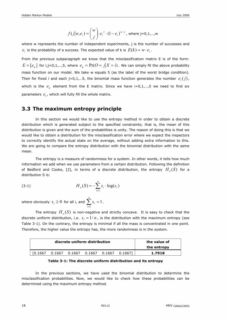
There are a significant number of transitions of the above type in the data. It means
that very often the error between the observed condition and the actual state of a bridge can be
large. Therefore, we decided to consider a misclassification error matrix which is fully filled and
to use the above type of the misclassification matrix only when we consider the data without so
big improvements in the conditions.
Finally the matrix E is of the following form:
=
555453525150
454443424140
353433323130
252423222120
151413121110
050403020100
eeeeeeeeeeeeeeeeeeeeeeeeeeeeeeeeeeeee
E
Misclassification matrix 3
There are several possibilities to specify the error probabilities: ije . One of them is
based on the binomial distribution, which is the subject of the subparagraph 3.2. Another way to specify these probabilities is the Maximum Entropy principle described in chapter 5. We will
consider also the misclassification matrix from the uniform distribution, i.e. in which each ije
is 1/6:
=
1667.01667.01667.01667.01667.01667.01667.01667.01667.01667.01667.01667.01667.01667.01667.01667.01667.01667.01667.01667.01667.01667.01667.01667.01667.01667.01667.01667.01667.01667.01667.01667.01667.01667.01667.01667.0
E
Uniform misclassification matrix
3.2 Binomial distribution for the misclassification parameters
Our task was to construct a model that accurately represents the experts’ error in
assessing the conditions of the bridges. In other words, we wanted to determine the conditional
probabilities of observations given the actual state in the way they fit the data well. The choice
for taking a binomial distribution to model the parameters was rather arbitrary. We were looking
for a discrete model which would generate the whole misclassification matrix E in a reasonable
way, but in the same time we wanted to minimize the number of necessary parameters to do it.
Since the matrix E is of the size 6 on 6, which implies 36 places to fill in (actually 30 places,
since the last number in each row must be chosen in a way that we get one by summing all the
values in the row).
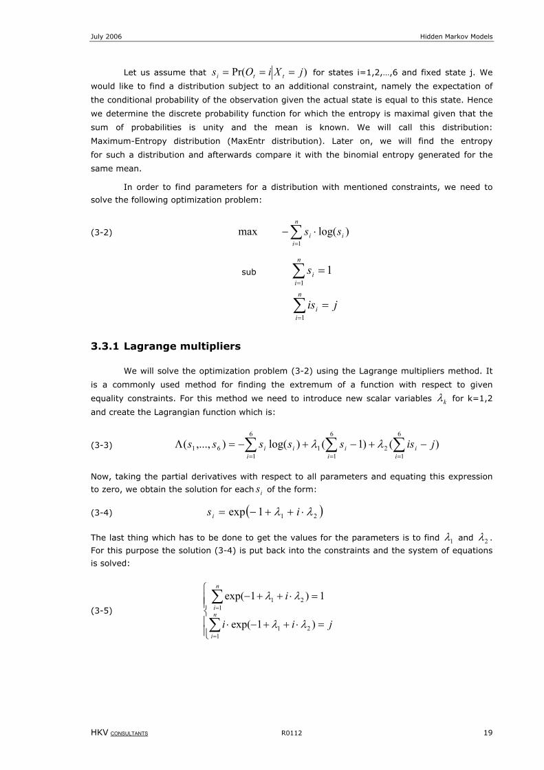
The binomial distribution gives a discrete probability distribution. The probability mass
function is given by the formula:
Hidden Markov Models July 2006
18 R0112 HKV CONSULTANTS
jwi
jii ee
jw
ewjf −−⋅⋅
= )1(),( , where j=0,1,…,w
where w represents the number of independent experiments, j is the number of successes and
ie is the probability of a success. The expected value of k is iewkE ⋅=)( .
From the previous subparagraph we know that the misclassification matrix E is of the form:
][ ijeE = for i,j=0,1,…,5, where )Pr( iXjOeij === . We can simply fit the above probability
mass function on our model. We take w equals 5 (as the label of the worst bridge condition).
Then for fixed i and each j=0,1,…5, the binomial mass function generates the number )( jei ,
which is the ije element from the E matrix. Since we have i=0,1,…,5 we need to find six
parameters ie , which will fully fill the whole matrix.
3.3 The maximum entropy principle
In this section we would like to use the entropy method in order to obtain a discrete
distribution which is generated subject to the specified constraints; that is, the mean of this
distribution is given and the sum of the probabilities is unity. The reason of doing this is that we
would like to obtain a distribution for the misclassification error where we expect the inspectors
to correctly identify the actual state on the average, without adding extra information to this.
We are going to compare the entropy distribution with the binomial distribution with the same
mean.
The entropy is a measure of randomness for a system. In other words, it tells how much
information we add when we use parameters from a certain distribution. Following the definition
of Bedford and Cooke, [2], in terms of a discrete distribution, the entropy )(SHn for a
distribution S is:
(3-1) ∑=
⋅−=n
iiin ssSH
1)log()(
where obviously 0≥is for all i, and ∑=
=n
iis
11 .
The entropy )(SHn is non-negative and strictly concave. It is easy to check that the
discrete uniform distribution, i.e. nsi /1= , is the distribution with the maximum entropy (see
Table 3-1). On the contrary, the entropy is minimal if all the mass is concentrated in one point.
Therefore, the higher value the entropy has, the more randomness is in the system.
discrete uniform distribution the value of
the entropy
[0.1667 0.1667 0.1667 0.1667 0.1667 0.1667] 1.7918
Table 3-1: The discrete uniform distribution and its entropy
In the previous sections, we have used the binomial distribution to determine the
misclassification probabilities. Now, we would like to check how these probabilities can be
determined using the maximum entropy method.
July 2006 Hidden Markov Models
HKV CONSULTANTS R0112 19
Let us assume that )Pr( jXiOs tti === for states i=1,2,…,6 and fixed state j. We
would like to find a distribution subject to an additional constraint, namely the expectation of
the conditional probability of the observation given the actual state is equal to this state. Hence
we determine the discrete probability function for which the entropy is maximal given that the
sum of probabilities is unity and the mean is known. We will call this distribution:
Maximum-Entropy distribution (MaxEntr distribution). Later on, we will find the entropy
for such a distribution and afterwards compare it with the binomial entropy generated for the
same mean.
In order to find parameters for a distribution with mentioned constraints, we need to
solve the following optimization problem:
(3-2) )log(max1
i
n
ii ss ⋅− ∑
=
sub ∑=
=n
iis
11
∑=
=n
ii jis
1
3.3.1 Lagrange multipliers
We will solve the optimization problem (3-2) using the Lagrange multipliers method. It
is a commonly used method for finding the extremum of a function with respect to given
equality constraints. For this method we need to introduce new scalar variables kλ for k=1,2
and create the Lagrangian function which is:
(3-3) )()1()log(),...,(6
12
6
1
6
1161 ∑∑ ∑
== =
−+−+−=Λi
ii i
iii jissssss λλ
Now, taking the partial derivatives with respect to all parameters and equating this expression
to zero, we obtain the solution for each is of the form:
(3-4) ( )211exp λλ ⋅++−= isi
The last thing which has to be done to get the values for the parameters is to find 1λ and 2λ .
For this purpose the solution (3-4) is put back into the constraints and the system of equations
is solved:
(3-5)
=⋅++−⋅
=⋅++−
∑
∑
=
=
jii
in
i
n
i
121
121
)1exp(
1)1exp(
λλ
λλ
Hidden Markov Models July 2006
20 R0112 HKV CONSULTANTS
(3-5) can be transformed to:
(3-6)
−⋅=⋅⋅
−=⋅
∑
∑
=
=
)1exp()exp(
)1exp()exp(
11
2
112
λλ
λλ
jii
in
i
n
i
(3-6) is equivalent with (3-7):
(3-7)
−=⋅⋅
−=⋅
∑
∑
=
=n
i
n
i
iij
i
112
11
2
)1exp()exp(1
)1exp()exp(
λλ
λλ
Equating both left sides of (3-7) we obtain the expression for the parameter 2λ :
(3-8) 0)1()exp(11
12 =−+⋅⋅+− ∑
−
=
jiijn
iλ
Furthermore, from the first equation of (3-6) we get:
(3-9) )1exp())exp(1(
))1exp(()exp(1
2
22 λλ
λλ−=
−⋅+− n
which follows that the parameter 1λ is expressed as:
(3-10) ))exp(1
))1exp(()exp(log(12
221 λ
λλλ
−⋅+−
−=n
Having the expression for 1λ , we can express the probability is as a function of 2λ as follows:
(3-11)
∑=
⋅
⋅=
⋅−−
⋅⋅
= n
i
i
i
in
is
12
2
2
2
2
2
)exp(
)exp()exp(1
)exp(1)exp()exp(
λ
λλ
λλλ
Since it is not possible to find those values explicitly we use the numerical method of
Newton-Raphson to work out the problem.
3.3.2 Newton-Raphson method
Newton-Raphson method (also called Newton’s method or Newton-Fourier method) is
a numerical algorithm, which uses the Taylor series, for finding approximations to the roots of
a real valued function. The first order Taylor approximation to a function )(xf about the point
ε+= 0xx is given by:
July 2006 Hidden Markov Models
HKV CONSULTANTS R0112 21
(3-12) εε ⋅+≈+ )(')()( 000 xfxfxf
Setting )( 0 ε+xf equal zero and solving for 0εε ≡ , we obtain the expression:
(3-13) )(')(
0
00 xf
xf−=ε
which is used to update the initial guess 0x . By letting 001 ε+= xx , calculating a new 1ε , and
so on, the process can be updated until it converges to a root using:
(3-14) )(')(
n
nn xf
xf−=ε
Hence the iterative formula for finding the root is:
(3-15) nnn xx ε+=+1
In our case, we define a function )( 2λf as the formula (5-8) reads:
(3-16) )1()exp(1)(1
122 jiijf
n
i−+⋅⋅+−= ∑
−
=
λλ
and we apply the Newton’s iterative algorithm to get the values for 2λ . Once, we obtain this
value, the parameter 1λ is calculated straightforward from the formula (3-10). Then those
values are used to determine the probabilities is for the MaxEntr distribution.
Unfortunately, the iterative method of Newton-Raphson has some drawbacks that need
to be avoided in order to make this method converge. First of all, a derivative of the function
requires to be expressed in explicit form. This is fulfilled here, since the derivative of (3-15)
reads:
(3-17) )1()exp()('1
122 jiiif
n
i−+⋅⋅⋅= ∑
−
=
λλ
However, the explicit form of the derivative does not guarantee the convergence. The
essential role plays the initial guess, which has to be chosen close ‘enough’ to the solution. If
the initial guess is too far from the true zero, this method can fail to converge. Anyway, in this
case the initial point is not extremely hard to be matched suitably. Therefore, we can still use
this method to find the parameter 2λ .
The method does not converge also near a horizontal asymptote and it cannot be used
for those cases. Therefore for j=1 and j=6 we need to find the solution without the numerical
scheme. For j=1 and j=6, we assume that the mass of the MaxEntr distribution is concentrated
in one point.
Hidden Markov Models July 2006
22 R0112 HKV CONSULTANTS
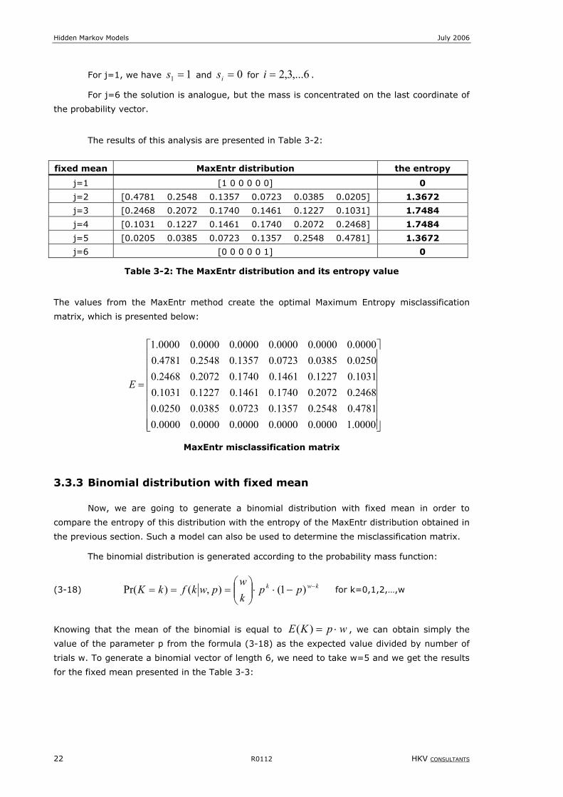
For j=1, we have 11 =s and 0=is for 6,...3,2=i .
For j=6 the solution is analogue, but the mass is concentrated on the last coordinate of
the probability vector.
The results of this analysis are presented in Table 3-2:
fixed mean MaxEntr distribution the entropy
j=1 [1 0 0 0 0 0] 0
j=2 [0.4781 0.2548 0.1357 0.0723 0.0385 0.0205] 1.3672
j=3 [0.2468 0.2072 0.1740 0.1461 0.1227 0.1031] 1.7484
j=4 [0.1031 0.1227 0.1461 0.1740 0.2072 0.2468] 1.7484
j=5 [0.0205 0.0385 0.0723 0.1357 0.2548 0.4781] 1.3672
j=6 [0 0 0 0 0 1] 0
Table 3-2: The MaxEntr distribution and its entropy value
The values from the MaxEntr method create the optimal Maximum Entropy misclassification
matrix, which is presented below:
=
0000.10000.00000.00000.00000.00000.04781.02548.01357.00723.00385.00250.02468.02072.01740.01461.01227.01031.01031.01227.01461.01740.02072.02468.00250.00385.00723.01357.02548.04781.00000.00000.00000.00000.00000.00000.1
E
MaxEntr misclassification matrix
3.3.3 Binomial distribution with fixed mean
Now, we are going to generate a binomial distribution with fixed mean in order to
compare the entropy of this distribution with the entropy of the MaxEntr distribution obtained in
the previous section. Such a model can also be used to determine the misclassification matrix.
The binomial distribution is generated according to the probability mass function:
(3-18) kwk ppkw
pwkfkK −−⋅⋅
=== )1(),()Pr( for k=0,1,2,…,w
Knowing that the mean of the binomial is equal to wpKE ⋅=)( , we can obtain simply the
value of the parameter p from the formula (3-18) as the expected value divided by number of
trials w. To generate a binomial vector of length 6, we need to take w=5 and we get the results
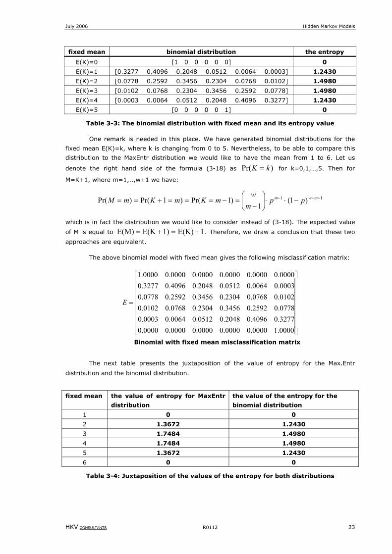
for the fixed mean presented in the Table 3-3:
July 2006 Hidden Markov Models
HKV CONSULTANTS R0112 23
fixed mean binomial distribution the entropy
E(K)=0 [1 0 0 0 0 0] 0
E(K)=1 [0.3277 0.4096 0.2048 0.0512 0.0064 0.0003] 1.2430
E(K)=2 [0.0778 0.2592 0.3456 0.2304 0.0768 0.0102] 1.4980
E(K)=3 [0.0102 0.0768 0.2304 0.3456 0.2592 0.0778] 1.4980
E(K)=4 [0.0003 0.0064 0.0512 0.2048 0.4096 0.3277] 1.2430
E(K)=5 [0 0 0 0 0 1] 0
Table 3-3: The binomial distribution with fixed mean and its entropy value
One remark is needed in this place. We have generated binomial distributions for the
fixed mean E(K)=k, where k is changing from 0 to 5. Nevertheless, to be able to compare this
distribution to the MaxEntr distribution we would like to have the mean from 1 to 6. Let us
denote the right hand side of the formula (3-18) as )Pr( kK = for k=0,1,…,5. Then for
M=K+1, where m=1,..,w+1 we have:
11 )1(1
)1Pr()1Pr()Pr( +−− −⋅⋅
−
=−===+== mwm ppmw
mKmKmM
which is in fact the distribution we would like to consider instead of (3-18). The expected value
of M is equal to 1E(K)1)E(KE(M) +=+= . Therefore, we draw a conclusion that these two
approaches are equivalent.
The above binomial model with fixed mean gives the following misclassification matrix:
=
0000.10000.00000.00000.00000.00000.03277.04096.02048.00512.00064.00003.00778.02592.03456.02304.00768.00102.00102.00768.02304.03456.02592.00778.00003.00064.00512.02048.04096.03277.00000.00000.00000.00000.00000.00000.1
E
Binomial with fixed mean misclassification matrix
The next table presents the juxtaposition of the value of entropy for the Max.Entr
distribution and the binomial distribution.
fixed mean the value of entropy for MaxEntr
distribution
the value of the entropy for the
binomial distribution
1 0 0
2 1.3672 1.2430
3 1.7484 1.4980
4 1.7484 1.4980
5 1.3672 1.2430
6 0 0
Table 3-4: Juxtaposition of the values of the entropy for both distributions
Hidden Markov Models July 2006
24 R0112 HKV CONSULTANTS
From the Table 3-4 we can see that the binomial distribution has a smaller entropy than the
MaxEntr distribution. It means that the MaxEntr distribution brings in more uncertainty (i.e. less
information) into the stochastic model describing the deterioration process. However, the
entropy measures how the given distributions are spread out with respect to the uniform
distribution. To check the precise relation between both distributions we will use the relative
information principle.
3.4 The relative information principle
The relative information measures the relation between two distributions without
involving the uniform distribution. Thanks to this measure we can find how close one
distribution is to another. In terms of mathematical formula the relative information of b with
respect to s, is expressed as (Bedford and Cooke, [2]):
∑=
⋅=n
i i
ii s
bbsbI
1)log();(
where ][ ibb = is the binomial distribution and ][ iss = is the MaxEntr-distribution for our case.
The number );( sbI is always non-negative. It takes its minimal value of 0 when b=s.
Therefore, if two distributions are close to each other, what means that they bring comparable
information to a process, then their relative information is close to 0. However, this principle
requires the elements ib and is not to be equal 0. For this case we have that the relative
information goes to infinity.
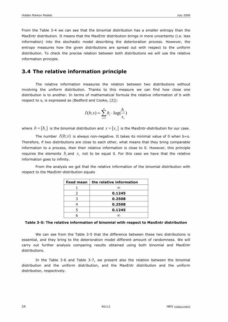
From the analysis we got that the relative information of the binomial distribution with
respect to the MaxEntr-distribution equals
fixed mean the relative information
1 ∞
2 0.1245
3 0.2508
4 0.2508
5 0.1245
6 ∞
Table 3-5: The relative information of binomial with respect to MaxEntr distribution
We can see from the Table 3-5 that the difference between these two distributions is
essential, and they bring to the deterioration model different amount of randomness. We will
carry out further analysis comparing results obtained using both binomial and MaxEntr
distributions.
In the Table 3-6 and Table 3-7, we present also the relation between the binomial
distribution and the uniform distribution, and the MaxEntr distribution and the uniform
distribution, respectively.

July 2006 Hidden Markov Models
HKV CONSULTANTS R0112 25
fixed mean the relative information
1 ∞
2 0.5489
3 0.2938
4 0.2938
5 0.5489
6 ∞
Table 3-6: The relative information of binomial with respect to uniform distribution
fixed mean the relative information
1 ∞
2 0.4243
3 0.0431
4 0.0431
5 0.4243
6 ∞
Table 3-7: The relative information of MaxEntr with respect to uniform distribution
From these results we can see that the Maximum Entropy distribution (MaxEntr) has
always smaller relative information with respect to the uniform distribution than the binomial
distribution with respect to the uniform distribution. Of course, it makes sense as the ‘maximum
entropy’ indicates that the distribution is close to the uniform, so it must introduce a similar
amount of randomness to the system. However, we can notice that for the mean ‘3’ and ‘4’ the
value of the relative information is close to zero. This means that those cases bring comparable
amount of uncertainty to the system.

July 2006 Hidden Markov Models
HKV CONSULTANTS R0112 27
4 Estimation of model parameters
In this chapter we would like to get the transition and the misclassification parameters
for our model. Before the mathematical model is presented, we need to describe in detail the
mechanism of the inspections.
The bridge inspections are carried out periodically. Therefore we do not have
information about their conditions at any time, but only at the specified points in time.
Predominantly, each structure was inspected two or three times, but for some of the structures
the number of inspections was higher, like for instance six times. As it was mentioned before,
we assume in this research that the ratings from experts are the observations, which are prone
to a bias. Therefore, we consider expert observations and the corresponding actual states for
each observation. We will denote the k-th observation for the i-th structure as ikO for k=1,…,m,
where m is the number of observations for the particular structure i. Moreover, ikO means that
the k-th inspection is carried out at time kt and the corresponding actual state kX is the real
condition of the bridge at the same time kt .
4.1 The Maximum Likelihood Estimation (MLE)
Once a model is specified with its parameters, the evaluation of its goodness of fit must
be determined. Goodness of fit is assessed by finding values of the parameters of the model
that best fit the data. This procedure is called parameter estimation.
One of the most popular and commonly used methods for estimating unknown
parameters is maximum-likelihood estimation. A likelihood function is the probability density
function of the data regarded as a function of the statistical parameters. The maximum
likelihood estimators are the values of the parameters that maximize the likelihood function. We
would like to use this method to estimate the parameters for the transition matrix and the
misclassification matrix. The matrix product method to calculate the likelihood function, which
was proposed by Jackson et al [1], is used here to estimate the parameters of the model for the
bridges in the Netherlands.
Consider a family of probability functions, say ),( θ⋅Xf . The likelihood function of a
random sample of size n from the population ),( θ⋅Xf is the joint probability density function
of the sample variables regarded as a function of the parameter θ . In mathematical
formulation:
(4-1) ∏=
=n
iiX xfxL
1
),(),( θθ
A maximum likelihood estimate (MLE) of θ is a value of θ̂ such that for all θ :
),()ˆ,( θθ xLxL ≥
([4], Gibbons, Chakraborti, 1992).
Often it is more convenient to use the log-likelihood function, because logarithms
transform products into sums, and maximizing the log-likelihood function is equivalent to
maximizing the likelihood function.
Hidden Markov Models July 2006
28 R0112 HKV CONSULTANTS
The data supplies information about the number of inspections for each of the bridge
and about the results of those inspections on a discrete scale. Thus, for each bridge we have a
sequence of observations: ,,...,,, 321im
iii OOOO where i indicates the bridge index and m is the
number of observations for the bridge. Therefore, every bridge i contributes to the likelihood
function in the following way:
(4-2) ===== ),...,,Pr()( 2211 mim
iii jOjOjOL θ
),...,Pr(),...,,...,Pr( 111111 mim
im
im
im
im
i lXlXlXlXjOjO ==⋅===== ∑
where the sum is taken over all possible paths of the actual states and }5,...,2,1,0{, ∈mm lj are
the values from the state sets.
Here, we need to use the assumption of conditional independence of the observations
given the values of actual states. Also, we use the Markov property, and then we can write
(4-2) in the form (for a proof, see Appendix B):
(4-3) ∑∑==
⋅====⋅====5
01122222211
5
01111
2
)Pr()Pr()Pr()Pr()(l
iiiii
l
iii lXlXlXjOlXlXjOL
l
θ
∑∑=
−−=
====⋅⋅====5
011
5
022333333 )Pr()Pr(...)Pr()Pr(
3 mlm
imm
imm
imm
im
l
iiii lXlXlXjOlXlXlXjO
where )Pr( mimm
im lXjO == is the misclassification probability
mm jle for each bridge i, and
)Pr()(1111 −−− ===−
− m
imm
immmll lXlXttp
mm is the ),( 1 mm ll − entry of the transition probability
matrix in t steps, where 1−−= mm ttt .
The formula (4-3) is in fact a product of matrices. To show this, let if be the row
vector of the form:
)]5Pr()5Pr(),...,0Pr()0[Pr( 11111111 =⋅===⋅=== iiiiiii XXjOXXjOf
For k=2,3,…,m, let ikF be a 6 by 6 matrix with (r,s) entry: )(
1−−⋅
kkk jjrssj ttpe , and let
1 be a column vector of size 6, consisting of 1s. Then the likelihood function for one object reads:
(4-4) 1...)( 32 ⋅⋅⋅⋅⋅= im
iiii FFFfL θ
For convenience we will work with the log-likelihood function:
(4-5) )1...log()(log)( 32 ⋅⋅⋅⋅⋅== im
iiiii FFFfLl θθ
Having the likelihood function for one object we can derive the likelihood for the whole
data. Let N be the number of objects in our data. Then:
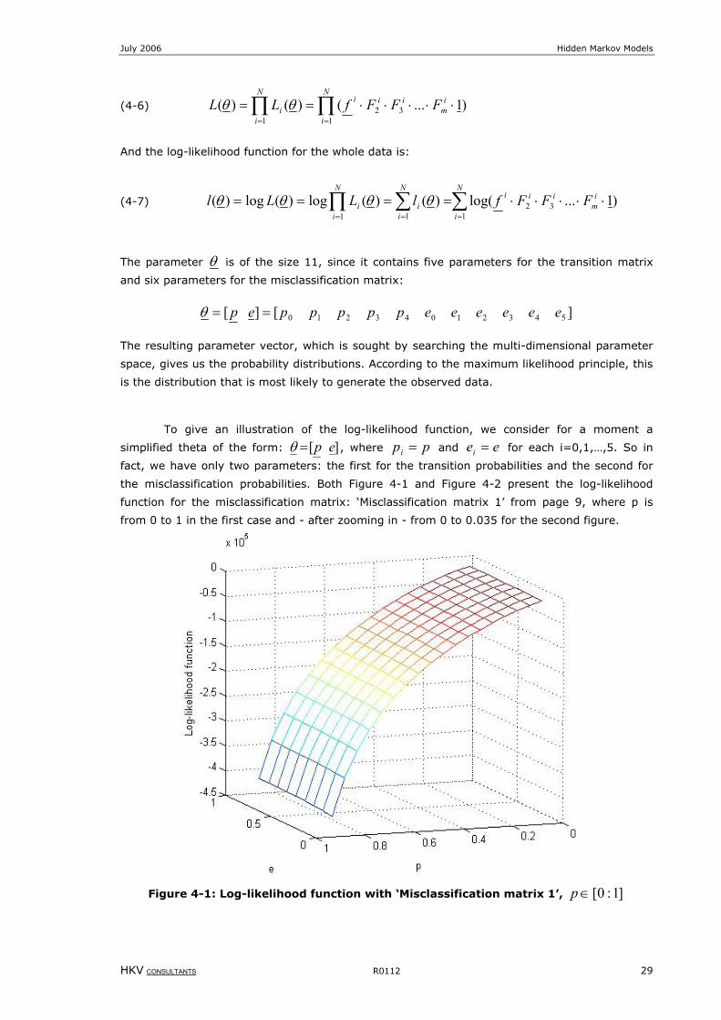
July 2006 Hidden Markov Models
HKV CONSULTANTS R0112 29
(4-6) ∏∏==
⋅⋅⋅⋅⋅==N
i
im
iiiN
ii FFFfLL
132
1
)1...()()( θθ
And the log-likelihood function for the whole data is:
(4-7) ∑∑∏===
⋅⋅⋅⋅⋅====N
i
im
iiiN
ii
N
ii FFFflLLl
132
11
)1...log()()(log)(log)( θθθθ
The parameter θ is of the size 11, since it contains five parameters for the transition matrix
and six parameters for the misclassification matrix:
][][ 54321043210 eeeeeepppppep ==θ
The resulting parameter vector, which is sought by searching the multi-dimensional parameter
space, gives us the probability distributions. According to the maximum likelihood principle, this
is the distribution that is most likely to generate the observed data.
To give an illustration of the log-likelihood function, we consider for a moment a
simplified theta of the form: ][ ep=θ , where ppi = and eei = for each i=0,1,…,5. So in
fact, we have only two parameters: the first for the transition probabilities and the second for
the misclassification probabilities. Both Figure 4-1 and Figure 4-2 present the log-likelihood
function for the misclassification matrix: ‘Misclassification matrix 1’ from page 9, where p is
from 0 to 1 in the first case and - after zooming in - from 0 to 0.035 for the second figure.
Figure 4-1: Log-likelihood function with ‘Misclassification matrix 1’, ]1:0[∈p
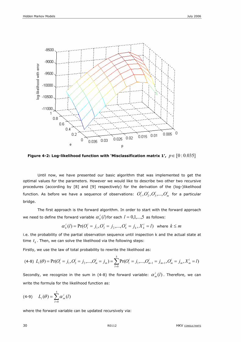
Hidden Markov Models July 2006
30 R0112 HKV CONSULTANTS
Figure 4-2: Log-likelihood function with ‘Misclassification matrix 1’, ]035.0:0[∈p
Until now, we have presented our basic algorithm that was implemented to get the
optimal values for the parameters. However we would like to describe two other two recursive
procedures (according by [8] and [9] respectively) for the derivation of the (log-)likelihood
function. As before we have a sequence of observations: im
iii OOOO ,...,,, 321 for a particular
bridge.
The first approach is the forward algorithm. In order to start with the forward approach
we need to define the forward variable )(likα for each 5,...,1,0=l as follows:
),,...,,Pr()( 2211 lXjOjOjOl ikk
ik
iiik =====α where mk ≤
i.e. the probability of the partial observation sequence until inspection k and the actual state at
time kt . Then, we can solve the likelihood via the following steps:
Firstly, we use the law of total probability to rewrite the likelihood as:
(4-8) ∑=
−− =========5
011112211 ),,,...,Pr(),...,,Pr()(
l
imm
imm
im
im
im
iii lXjOjOjOjOjOjOL θ
Secondly, we recognize in the sum in (4-8) the forward variable: )(limα . Therefore, we can
write the formula for the likelihood function as:
(4-9) ∑=
=5
0)()(
l
imi lL αθ
where the forward variable can be updated recursively via:
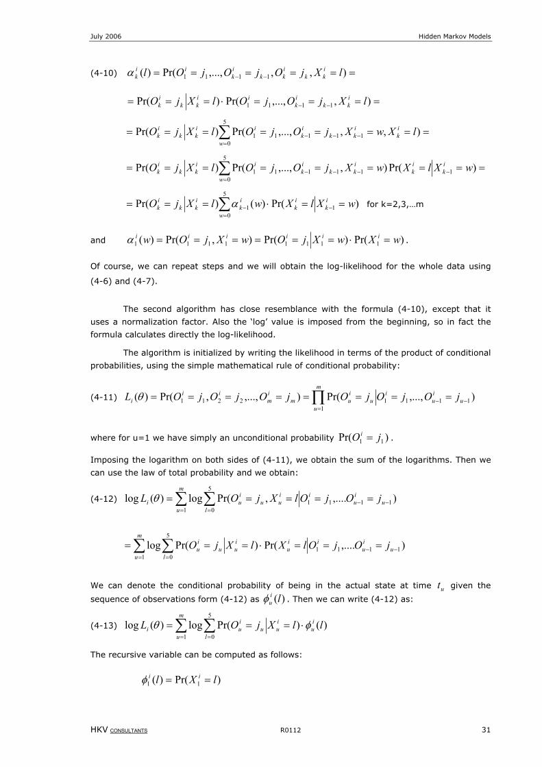
July 2006 Hidden Markov Models
HKV CONSULTANTS R0112 31
(4-10) ====== −− ),,,...,Pr()( 1111 lXjOjOjOl ikk
ikk
ik
iikα
====⋅=== −− ),,...,Pr()Pr( 1111 lXjOjOlXjO ikk
ik
iikk
ik
======== ∑=
−−−
5
011111 ),,,...,Pr()Pr(
w
ik
ikk
ik
iikk
ik lXwXjOjOlXjO
========= ∑=
−−−−
5
0111111 )Pr(),,...,Pr()Pr(
w
ik
ik
ikk
ik
iikk
ik wXlXwXjOjOlXjO
∑=
−− ==⋅===5
011 )Pr()()Pr(
w
ik
ik
ik
ikk
ik wXlXwlXjO α for k=2,3,…m
and )Pr()Pr(),Pr()( 11111111 wXwXjOwXjOw iiiiii =⋅======α .
Of course, we can repeat steps and we will obtain the log-likelihood for the whole data using
(4-6) and (4-7).
The second algorithm has close resemblance with the formula (4-10), except that it
uses a normalization factor. Also the ‘log’ value is imposed from the beginning, so in fact the
formula calculates directly the log-likelihood.
The algorithm is initialized by writing the likelihood in terms of the product of conditional
probabilities, using the simple mathematical rule of conditional probability:
(4-11) ∏=
−− ========m
uu
iu
iu
ium
im
iii jOjOjOjOjOjOL
111112211 ),...,Pr(),...,,Pr()(θ
where for u=1 we have simply an unconditional probability )Pr( 11 jOi = .
Imposing the logarithm on both sides of (4-11), we obtain the sum of the logarithms. Then we
can use the law of total probability and we obtain:
(4-12) ∑ ∑= =
−− =====m
u lu
iu
iiuu
iui jOjOlXjOL
1
5
01111 ),....,Pr(log)(log θ
∑ ∑= =
−− ===⋅===m
u lu
iu
iiu
iuu
iu jOjOlXlXjO
1
5
01111 ),....Pr()Pr(log
We can denote the conditional probability of being in the actual state at time ut given the
sequence of observations form (4-12) as )(liuφ . Then we can write (4-12) as:
(4-13) ∑ ∑= =
⋅===m
u
iu
l
iuu
iui llXjOL
1
5
0)()Pr(log)(log φθ
The recursive variable can be computed as follows:
)Pr()( 11 lXl ii ==φ
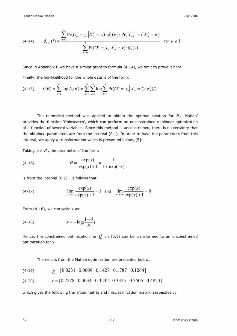
Hidden Markov Models July 2006
32 R0112 HKV CONSULTANTS
(4-14)
∑
∑
=
+=
+
⋅==
==⋅⋅=== 5
0
1
5
01
)()Pr(
)Pr()()Pr()(
v
iu
iuu
iu
iu
iu
iu
w
iuu
iu
iu
vvXjO
wXlXwwXjOl
φ
φφ for 1≥u
Since in Appendix B we have a similar proof to formula (4-14), we omit to prove it here.
Finally, the log-likelihood for the whole data is of the form:
(4-15) ∑∑ ∑∑= = ==
⋅====N
i
m
u
iu
l
iuu
iu
N
ii llXjOLL
1 1
5
01)()Pr(log)(log)( φθθ
The numerical method was applied to obtain the optimal solution for θ . ‘Matlab’
provides the function ‘fminsearch’, which can perform an unconstrained nonlinear optimization
of a function of several variables. Since this method is unconstrained, there is no certainty that
the obtained parameters are from the interval (0,1). In order to have the parameters from this
interval, we apply a transformation which is presented below, [5]:
Taking Rx∈ , the parameter of the form:
(4-16) )exp(1
11)exp(
)exp(xx
x−+
=+
=θ
is from the interval (0,1). It follows that:
(4-17) 11)exp(
)exp(lim =++∞→ xx
x and 0
1)exp()exp(lim =+−∞→ xx
x
From (4-16), we can write x as:
(4-18) )1log(θ
θ−−=x
Hence, the constrained optimization for θ on (0,1) can be transformed to an unconstrained
optimization for x.
The results from the Matlab optimization are presented below:
(4-19) ]0.1264 0.1787 0.1427 0.0609 0.0231[=p
(4-20) ]0.4823 0.3505 0.3325 0.3242 0.3034 0.2278[=e
which gives the following transition matrix and misclassification matrix, respectively:
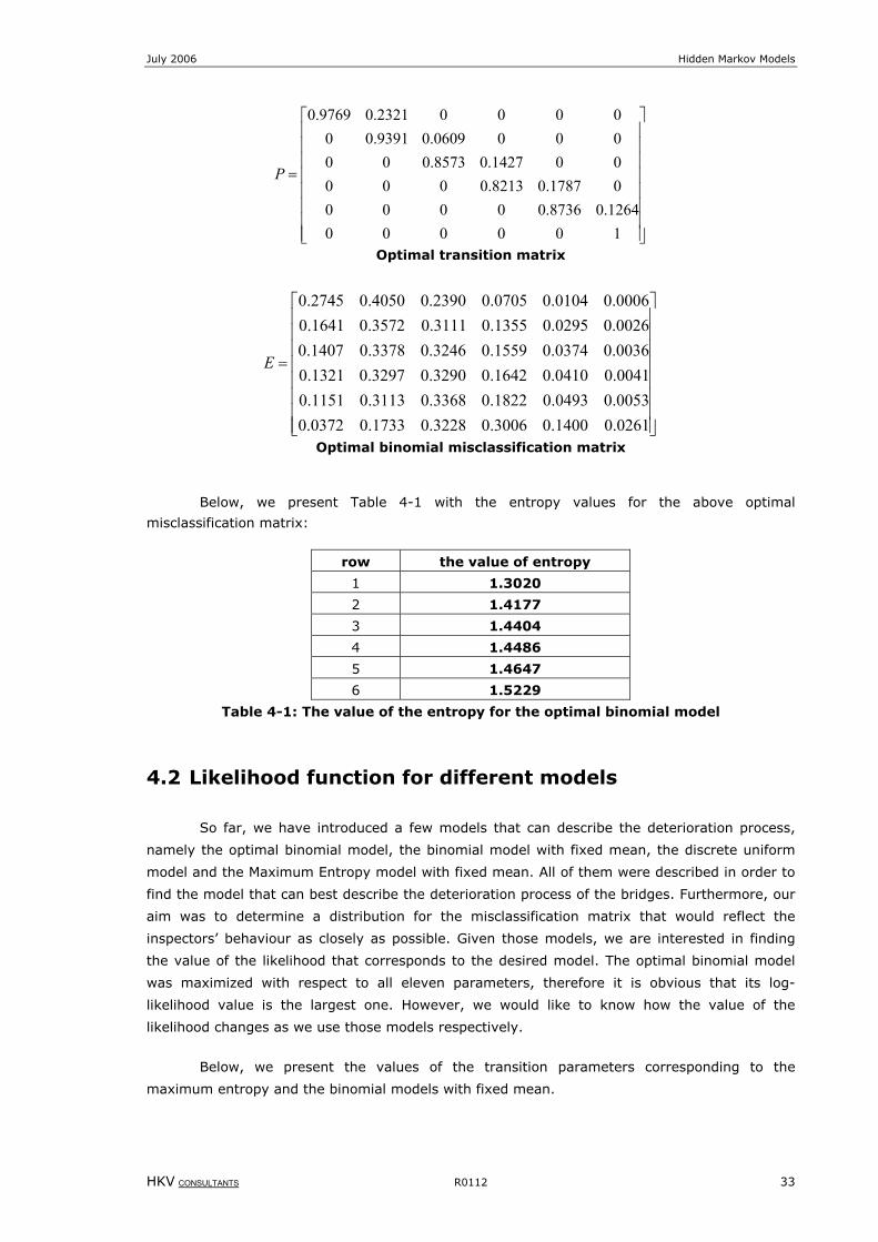
July 2006 Hidden Markov Models
HKV CONSULTANTS R0112 33
=
1000001264.08736.0000001787.08213.0000001427.08573.0000000609.09391.0000002321.09769.0
P
Optimal transition matrix
=
0261.01400.03006.03228.01733.00372.00053.00493.01822.03368.03113.01151.00041.00410.01642.03290.03297.01321.00036.00374.01559.03246.03378.01407.00026.00295.01355.03111.03572.01641.00006.00104.00705.02390.04050.02745.0
E
Optimal binomial misclassification matrix
Below, we present Table 4-1 with the entropy values for the above optimal
misclassification matrix:
row the value of entropy
1 1.3020
2 1.4177
3 1.4404
4 1.4486
5 1.4647
6 1.5229
Table 4-1: The value of the entropy for the optimal binomial model
4.2 Likelihood function for different models
So far, we have introduced a few models that can describe the deterioration process,
namely the optimal binomial model, the binomial model with fixed mean, the discrete uniform
model and the Maximum Entropy model with fixed mean. All of them were described in order to
find the model that can best describe the deterioration process of the bridges. Furthermore, our
aim was to determine a distribution for the misclassification matrix that would reflect the
inspectors’ behaviour as closely as possible. Given those models, we are interested in finding
the value of the likelihood that corresponds to the desired model. The optimal binomial model
was maximized with respect to all eleven parameters, therefore it is obvious that its log-
likelihood value is the largest one. However, we would like to know how the value of the
likelihood changes as we use those models respectively.
Below, we present the values of the transition parameters corresponding to the
maximum entropy and the binomial models with fixed mean.

Hidden Markov Models July 2006
34 R0112 HKV CONSULTANTS
Model: maximum entropy with fixed mean
(4-21) ]0.0000 0.0000 0.0000 0.0551 0.4537[=p
Model: binomial with fixed mean
(4-22) ]0.0000 0.0000 0.0010 0.0416 0.3232[=p
These values indeed do not satisfy our expectation about them. We would rather expect
to obtain numbers different than zeros as they indicate the probabilities of moving to the next
states. With such values we get that the actual process stops at the state ‘2’ and ‘3’,
respectively, for those models. However, with the fully filled misclassification matrix E, even
with such parameters, it is still possible to observe any condition from the whole range of the
discrete scale.
The reason for such results can be in the data. The data contains a disproportionately
high amount of data concerning bridges below mediocre condition (condition 4) relatively to the
small number of data concerning bridges assessed as 4 and 5. This can influence the model a
lot. If we look at the misclassification matrix generated for the optimal binomial model, we can
see that the probability of observing the lower conditions is always very small and the highest
probabilities are concentrated in the left part of the matrix. This is in opposite to the models
with fixed means where more weights are assigned to the right part of the E matrix, especially
in the lower part of this matrix.
Here we should present also the transition parameters for the discrete uniform
distribution. However, during the analysis we noticed that those parameters do not influence the
value of the likelihood. It means that no matter how those parameters are, the value of the
likelihood stays always the same. The explanation of this fact will be given in the next chapter in
terms of the expected value of the observation at time t.
Table 4-2 presents the values of the likelihood for all mentioned models. From the table
we can see that the values differ significantly.
model log-likelihood value
optimal binomial -7257.70 binomial with fixed mean -8458.68 Max.Entr -10497.60
discrete uniform -9728.17
Table 4-2: The values of the log-likelihood functions
for different models (E-full)
We would like also to present the results from simulations for not fully filled
misclassification matrices: ‘Misclassification matrix 1’ and ‘Misclassification matrix 2’. The last
one was generated by the binomial model in a similar way as the full matrix. In order to obtain
the parameters we needed to delete from the data all transitions which result in the zero value
of the log-likelihood. This results in higher log-likelihood values, such that tables 4-2 and 4-3
can not be directly compared.
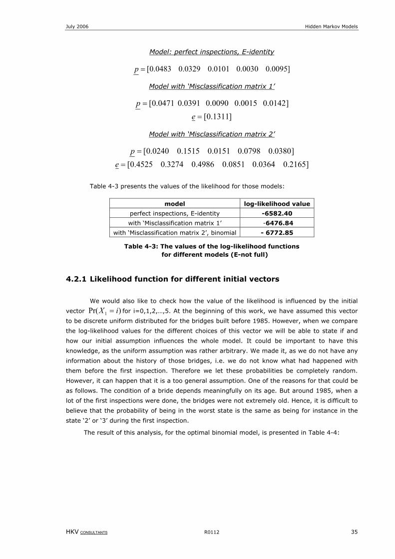
July 2006 Hidden Markov Models
HKV CONSULTANTS R0112 35
Model: perfect inspections, E-identity
]0095.00030.00101.00329.00483.0[=p
Model with ‘Misclassification matrix 1’
]0.0142 0.0015 0.0090 0.0391 0.0471[=p
]0.1311[=e
Model with ‘Misclassification matrix 2’
]0.0380 0.0798 0.0151 0.1515 0.0240[=p
]0.2165 0.0364 0.0851 0.4986 0.3274 0.4525[=e
Table 4-3 presents the values of the likelihood for those models:
model log-likelihood value
perfect inspections, E-identity -6582.40
with ‘Misclassification matrix 1’ -6476.84 with ‘Misclassification matrix 2’, binomial - 6772.85
Table 4-3: The values of the log-likelihood functions for different models (E-not full)
4.2.1 Likelihood function for different initial vectors
We would also like to check how the value of the likelihood is influenced by the initial
vector )Pr( 1 iX = for i=0,1,2,…,5. At the beginning of this work, we have assumed this vector
to be discrete uniform distributed for the bridges built before 1985. However, when we compare
the log-likelihood values for the different choices of this vector we will be able to state if and
how our initial assumption influences the whole model. It could be important to have this
knowledge, as the uniform assumption was rather arbitrary. We made it, as we do not have any
information about the history of those bridges, i.e. we do not know what had happened with
them before the first inspection. Therefore we let these probabilities be completely random.
However, it can happen that it is a too general assumption. One of the reasons for that could be
as follows. The condition of a bride depends meaningfully on its age. But around 1985, when a
lot of the first inspections were done, the bridges were not extremely old. Hence, it is difficult to
believe that the probability of being in the worst state is the same as being for instance in the
state ‘2’ or ‘3’ during the first inspection.
The result of this analysis, for the optimal binomial model, is presented in Table 4-4:

Hidden Markov Models July 2006
36 R0112 HKV CONSULTANTS
initial probabilities distribution log-likelihood
[0.1667 0.1667 0.1667 0.1667 0.1667 0.1667] Uniform(6) -7257.7
[0.3277 0.4096 0.2048 0.0512 0.0064 0.0003] Binomial, mean 1 -7345,1
[0.0778 0.2592 0.3456 0.2304 0.0768 0.0102] Binomial, mean 2 -7230.6
[0.0102 0.0768 0.2304 0.3456 0.2592 0.0778] Binomial, mean 3 -7213.3
[0.4780 0.2550 0.1350 0.0730 0.0385 0.0205] Max.Entr, mean 1 -7397.6
[0.2465 0.2075 0.1749 0.1450 0.1229 0.1031] Max.Entr, mean 2 -7280.0
[0.1031 0.1225 0.1460 0.1743 0.2079 0.2461] Max.Entr, mean 3 -7255,2
Table 4-4: The value of the likelihood for the different initial vector
From the above result, we can state that the choice of the initial vector does not play
a large role in both the values of log-likelihood as well as for the estimated parameters.
Therefore, we can assume it to be discrete uniformly distributed. However, we can see the
tendency that the value of the log-likelihood is rising up as the initial condition is more likely to
be better.
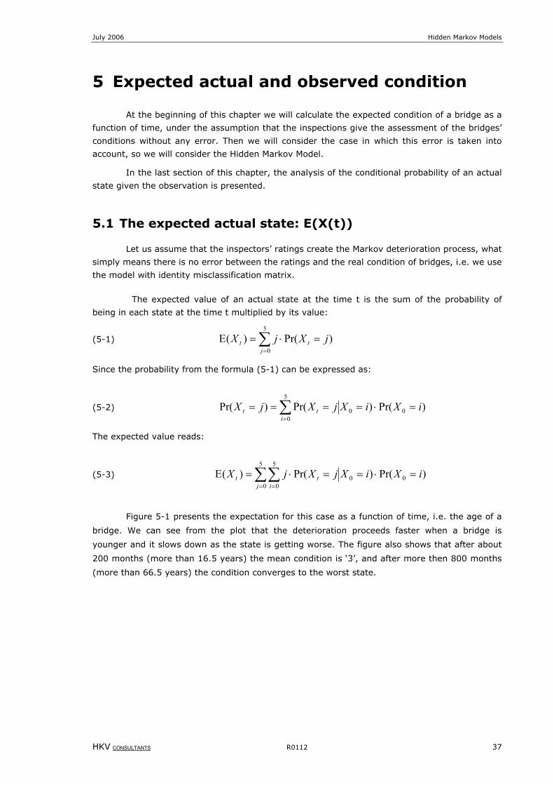
July 2006 Hidden Markov Models
HKV CONSULTANTS R0112 37
5 Expected actual and observed condition
At the beginning of this chapter we will calculate the expected condition of a bridge as a
function of time, under the assumption that the inspections give the assessment of the bridges’
conditions without any error. Then we will consider the case in which this error is taken into
account, so we will consider the Hidden Markov Model.
In the last section of this chapter, the analysis of the conditional probability of an actual
state given the observation is presented.
5.1 The expected actual state: E(X(t))
Let us assume that the inspectors’ ratings create the Markov deterioration process, what
simply means there is no error between the ratings and the real condition of bridges, i.e. we use
the model with identity misclassification matrix.
The expected value of an actual state at the time t is the sum of the probability of
being in each state at the time t multiplied by its value:
(5-1) ∑=
=⋅=Ε5
0)Pr()(
jtt jXjX
Since the probability from the formula (5-1) can be expressed as:
(5-2) ∑=
=⋅====5
000 )Pr()Pr()Pr(
itt iXiXjXjX
The expected value reads:
(5-3) ∑∑= =
=⋅==⋅=Ε5
00
5
00 )Pr()Pr()(
j itt iXiXjXjX
Figure 5-1 presents the expectation for this case as a function of time, i.e. the age of a
bridge. We can see from the plot that the deterioration proceeds faster when a bridge is
younger and it slows down as the state is getting worse. The figure also shows that after about
200 months (more than 16.5 years) the mean condition is ‘3’, and after more then 800 months
(more than 66.5 years) the condition converges to the worst state.
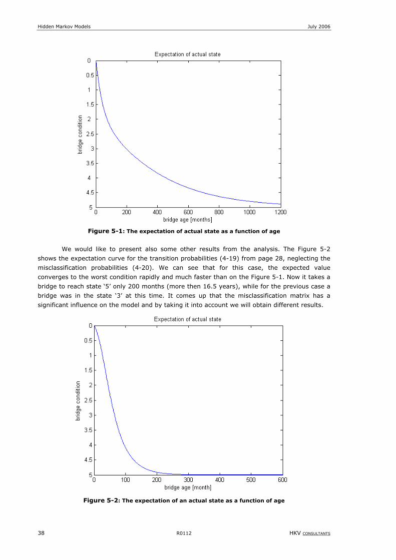
Hidden Markov Models July 2006
38 R0112 HKV CONSULTANTS
Figure 5-1: The expectation of actual state as a function of age
We would like to present also some other results from the analysis. The Figure 5-2
shows the expectation curve for the transition probabilities (4-19) from page 28, neglecting the
misclassification probabilities (4-20). We can see that for this case, the expected value
converges to the worst condition rapidly and much faster than on the Figure 5-1. Now it takes a
bridge to reach state ‘5’ only 200 months (more then 16.5 years), while for the previous case a
bridge was in the state ‘3’ at this time. It comes up that the misclassification matrix has a
significant influence on the model and by taking it into account we will obtain different results.
Figure 5-2: The expectation of an actual state as a function of age
July 2006 Hidden Markov Models
HKV CONSULTANTS R0112 39
Figure 5-3 presents the expectation for the Markov model (perfect inspections) but we
use modified data to obtain it. Now, the data contains information about the most severe bridge
damage. It means that the condition of a bridge depends on the condition of the worst part of
the bridge. We can see how much faster the expectation goes to the worst state comparing it to
the result in Figure 5-1. The expectation reaches state ‘5’ after 1000 months, while for the
previous case at time 1200 months it was close to this state, but still not exactly there. Besides,
we can see that for this model a bridge transits from perfect condition: ‘0’ to ‘1’ with probability
one, so in fact immediately. The explanation of this fact can be found after studying the data.
There are conditions ‘0’ only for new bridges (except one bridge with index 1440) and as soon
as an inspection takes place it never results in a rate better than ‘1’, but usually even worse.
There is only one exception (i.e. bridges with index 757). We attach some of the extreme cases
from this data in Appendix C. From those cases we can read that even a 4 month old bridges
can have already label ‘1,’ or even worse.
The transition parameters for this data are:
]0043.00072.00264.00454.01[=p
and the value of the log-likelihood function for this case is -4249.44. The value is much smaller
than before, since there is less data than in the regular data set.
Figure 5-3: The expectation of an actual state for the new data
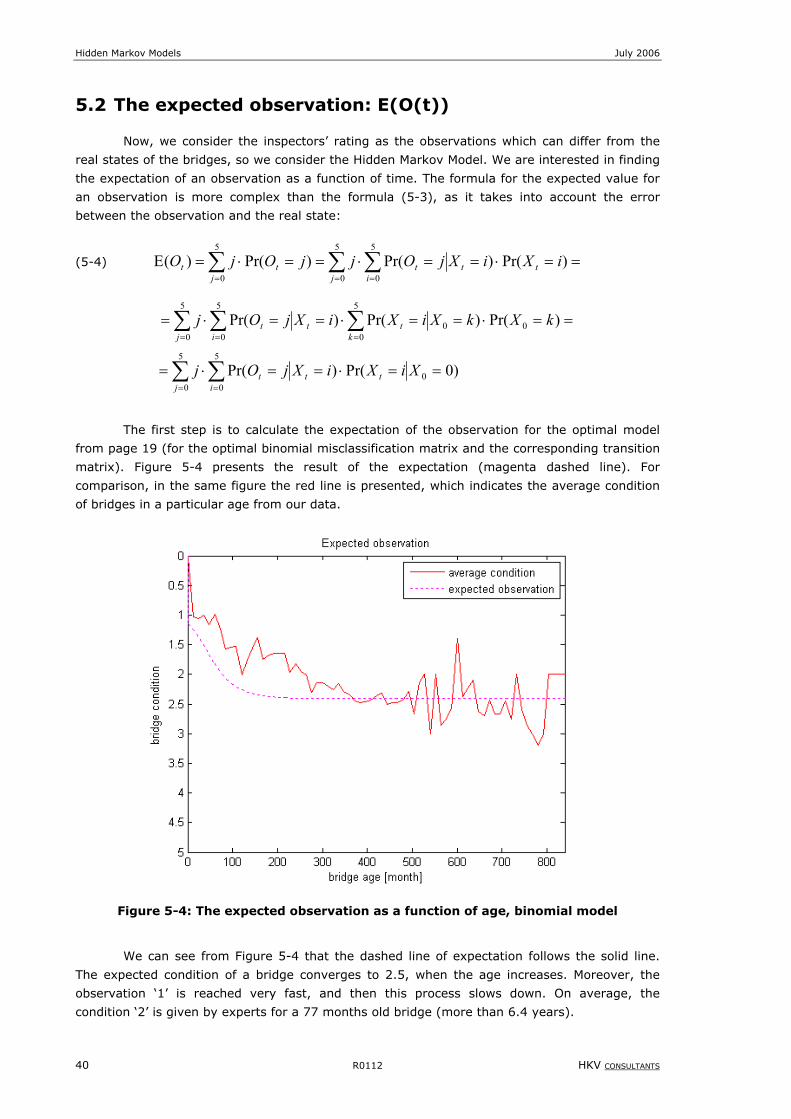
Hidden Markov Models July 2006
40 R0112 HKV CONSULTANTS
5.2 The expected observation: E(O(t))
Now, we consider the inspectors’ rating as the observations which can differ from the
real states of the bridges, so we consider the Hidden Markov Model. We are interested in finding
the expectation of an observation as a function of time. The formula for the expected value for
an observation is more complex than the formula (5-3), as it takes into account the error
between the observation and the real state:
(5-4) ==⋅==⋅==⋅=Ε ∑ ∑∑= ==
)Pr()Pr()Pr()(5
0
5
0
5
0iXiXjOjjOjO t
j itt
jtt
==⋅==⋅==⋅= ∑∑ ∑== =
)Pr()Pr()Pr( 0
5
00
5
0
5
0kXkXiXiXjOj
kt
j itt
)0Pr()Pr( 0
5
0
5
0==⋅==⋅= ∑ ∑
= =
XiXiXjOj tj i
tt
The first step is to calculate the expectation of the observation for the optimal model
from page 19 (for the optimal binomial misclassification matrix and the corresponding transition
matrix). Figure 5-4 presents the result of the expectation (magenta dashed line). For
comparison, in the same figure the red line is presented, which indicates the average condition
of bridges in a particular age from our data.
Figure 5-4: The expected observation as a function of age, binomial model
We can see from Figure 5-4 that the dashed line of expectation follows the solid line.
The expected condition of a bridge converges to 2.5, when the age increases. Moreover, the
observation ‘1’ is reached very fast, and then this process slows down. On average, the
condition ‘2’ is given by experts for a 77 months old bridge (more than 6.4 years).
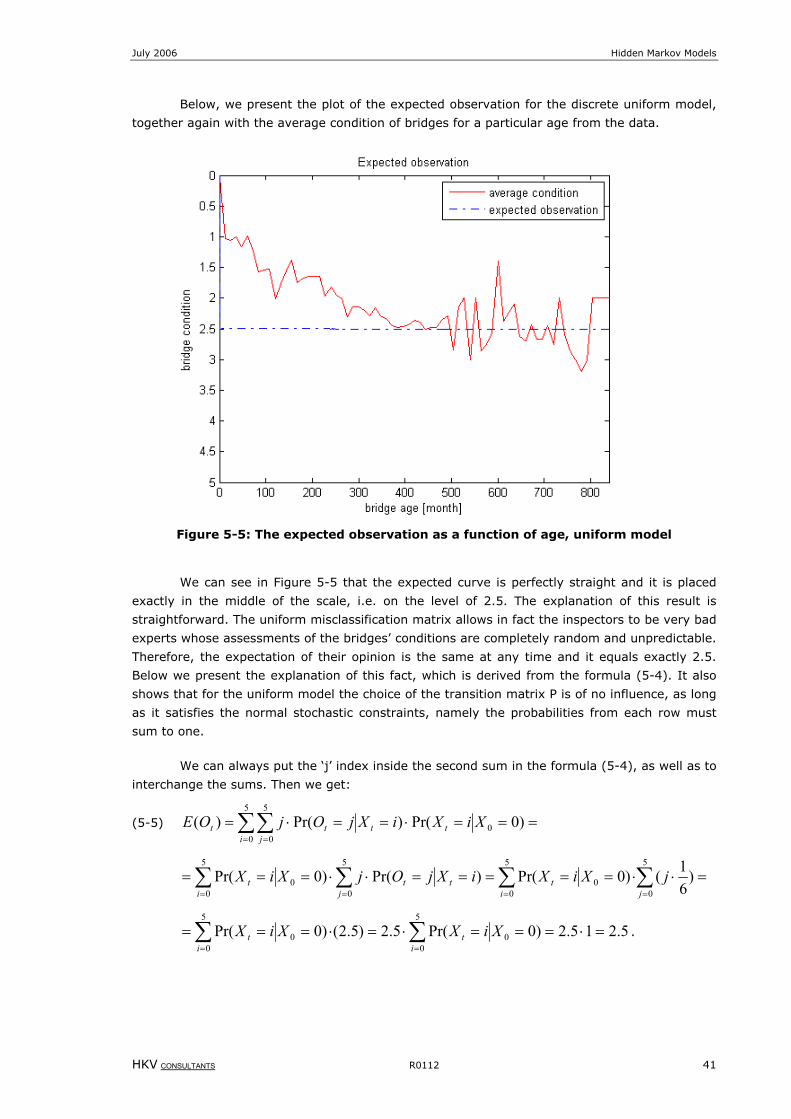
July 2006 Hidden Markov Models
HKV CONSULTANTS R0112 41
Below, we present the plot of the expected observation for the discrete uniform model,
together again with the average condition of bridges for a particular age from the data.
Figure 5-5: The expected observation as a function of age, uniform model
We can see in Figure 5-5 that the expected curve is perfectly straight and it is placed
exactly in the middle of the scale, i.e. on the level of 2.5. The explanation of this result is
straightforward. The uniform misclassification matrix allows in fact the inspectors to be very bad
experts whose assessments of the bridges’ conditions are completely random and unpredictable.
Therefore, the expectation of their opinion is the same at any time and it equals exactly 2.5.
Below we present the explanation of this fact, which is derived from the formula (5-4). It also
shows that for the uniform model the choice of the transition matrix P is of no influence, as long
as it satisfies the normal stochastic constraints, namely the probabilities from each row must
sum to one.
We can always put the ‘j’ index inside the second sum in the formula (5-4), as well as to
interchange the sums. Then we get:
(5-5) ===⋅==⋅= ∑∑= =
)0Pr()Pr()( 0
5
0
5
0XiXiXjOjOE t
i jttt
=⋅⋅=====⋅⋅=== ∑∑∑ ∑=== =
)61()0Pr()Pr()0Pr(
5
0
5
00
5
0
5
00
jit
i jttt jXiXiXjOjXiX
5.215.2)0Pr(5.2)5.2()0Pr(5
00
5
00 =⋅===⋅=⋅=== ∑∑
== it
it XiXXiX .
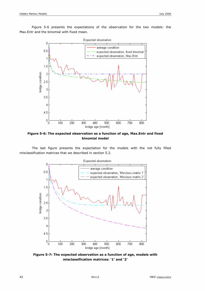
Hidden Markov Models July 2006
42 R0112 HKV CONSULTANTS
Figure 5-6 presents the expectations of the observation for the two models: the
Max.Entr and the binomial with fixed mean.
Figure 5-6: The expected observation as a function of age, Max.Entr and fixed
binomial model
The last figure presents the expectation for the models with the not fully filled
misclassification matrices that we described in section 5.2.
Figure 5-7: The expected observation as a function of age, models with
misclassification matrices: ‘1’ and ‘2’
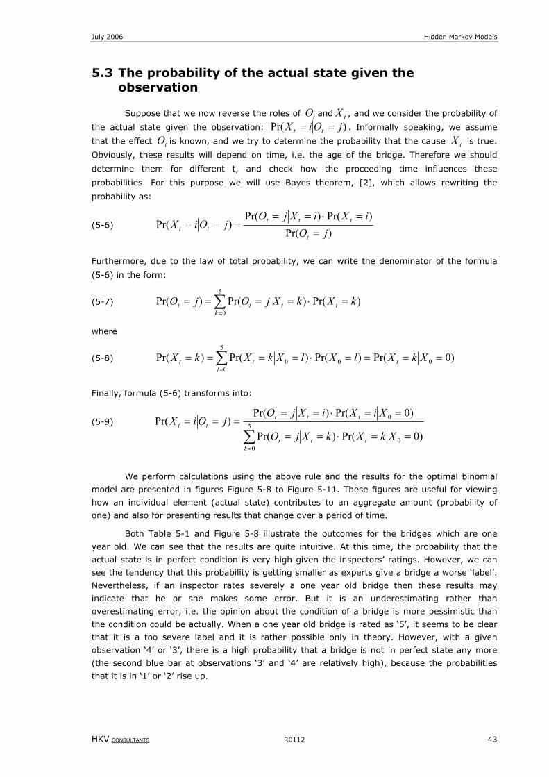
July 2006 Hidden Markov Models
HKV CONSULTANTS R0112 43
5.3 The probability of the actual state given the observation
Suppose that we now reverse the roles of tO and tX , and we consider the probability of
the actual state given the observation: )Pr( jOiX tt == . Informally speaking, we assume
that the effect tO is known, and we try to determine the probability that the cause tX is true.
Obviously, these results will depend on time, i.e. the age of the bridge. Therefore we should
determine them for different t, and check how the proceeding time influences these
probabilities. For this purpose we will use Bayes theorem, [2], which allows rewriting the
probability as:
(5-6) )Pr(
)Pr()Pr()Pr(
jOiXiXjO
jOiXt
ttttt =
=⋅=====
Furthermore, due to the law of total probability, we can write the denominator of the formula
(5-6) in the form:
(5-7) )Pr()Pr()Pr(5
0kXkXjOjO t
kttt =⋅==== ∑
=
where
(5-8) )0Pr()Pr()Pr()Pr( 00
5
00 ====⋅==== ∑
=
XkXlXlXkXkX tl
tt
Finally, formula (5-6) transforms into:
(5-9)
∑=
==⋅==
==⋅===== 5
00
0
)0Pr()Pr(
)0Pr()Pr()Pr(
kttt
ttttt
XkXkXjO
XiXiXjOjOiX
We perform calculations using the above rule and the results for the optimal binomial
model are presented in figures Figure 5-8 to Figure 5-11. These figures are useful for viewing
how an individual element (actual state) contributes to an aggregate amount (probability of
one) and also for presenting results that change over a period of time.
Both Table 5-1 and Figure 5-8 illustrate the outcomes for the bridges which are one
year old. We can see that the results are quite intuitive. At this time, the probability that the
actual state is in perfect condition is very high given the inspectors’ ratings. However, we can
see the tendency that this probability is getting smaller as experts give a bridge a worse ‘label’.
Nevertheless, if an inspector rates severely a one year old bridge then these results may
indicate that he or she makes some error. But it is an underestimating rather than
overestimating error, i.e. the opinion about the condition of a bridge is more pessimistic than
the condition could be actually. When a one year old bridge is rated as ‘5’, it seems to be clear
that it is a too severe label and it is rather possible only in theory. However, with a given
observation ‘4’ or ‘3’, there is a high probability that a bridge is not in perfect state any more
(the second blue bar at observations ‘3’ and ‘4’ are relatively high), because the probabilities
that it is in ‘1’ or ‘2’ rise up.

Hidden Markov Models July 2006
44 R0112 HKV CONSULTANTS
Figure 5-8: Probability of the actual state given the observation, t=12 months
X
O
0 1 2 3 4 5
0 0.8453 0.7819 0.7005 0.6022 0.4921 0.3702
1 0.1163 0.1588 0.2100 0.2665 0.3214 0.3694
2 0.0252 0.0378 0.0551 0.0771 0.1023 0.1288
3 0.0095 0.0148 0.0223 0.0324 0.0447 0.0586
4 0.0035 0.0059 0.0096 0.0152 0.0227 0.0320
5 0.0003 0.0009 0.0024 0.0065 0.0169 0.0410
Table 5-1: Probability of an actual state given the observation, t=12 months
After two years (24 months) the situation changes a bit. The probability of being in
state ‘0’ is still high, but smaller than before and the other probabilities rise up. Now, if an
inspector rates a bridge as for instance ‘3’, the probability that he or she assesses it correctly is
much higher than before. Nevertheless, a very likely scenario is that the actual condition is ‘5’,
or even more probably ‘0’ for this case. We can see that while the proportion for the
observations ‘0’ and ‘1’ does not change dramatically, the differences are visible for lower
labels. We can perceive the following tendency: assessment of the real state when it oscillates
around ‘3’ and ‘4’ is a difficult task, and we should be careful in trusting the inspectors’ rating in
this case. Furthermore, we can see in Figure 5-9 that if a bridge is rated as ‘5’ after two years,
there is about 0.38 probability that it is indeed in this condition.
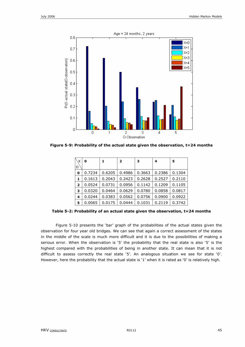
July 2006 Hidden Markov Models
HKV CONSULTANTS R0112 45
Figure 5-9: Probability of the actual state given the observation, t=24 months
X
O
0 1 2 3 4 5
0 0.7234 0.6205 0.4986 0.3663 0.2386 0.1304
1 0.1613 0.2043 0.2423 0.2628 0.2527 0.2110
2 0.0524 0.0731 0.0956 0.1142 0.1209 0.1105
3 0.0320 0.0464 0.0629 0.0780 0.0858 0.0817
4 0.0244 0.0383 0.0562 0.0756 0.0900 0.0922
5 0.0065 0.0175 0.0444 0.1031 0.2119 0.3742
Table 5-2: Probability of an actual state given the observation, t=24 months
Figure 5-10 presents the ‘bar’ graph of the probabilities of the actual states given the
observation for four year old bridges. We can see that again a correct assessment of the states
in the middle of the scale is much more difficult and it is due to the possibilities of making a
serious error. When the observation is ‘5’ the probability that the real state is also ‘5’ is the
highest compared with the probabilities of being in another state. It can mean that it is not
difficult to assess correctly the real state ‘5’. An analogous situation we see for state ‘0’.
However, here the probability that the actual state is ‘1’ when it is rated as ‘0’ is relatively high.
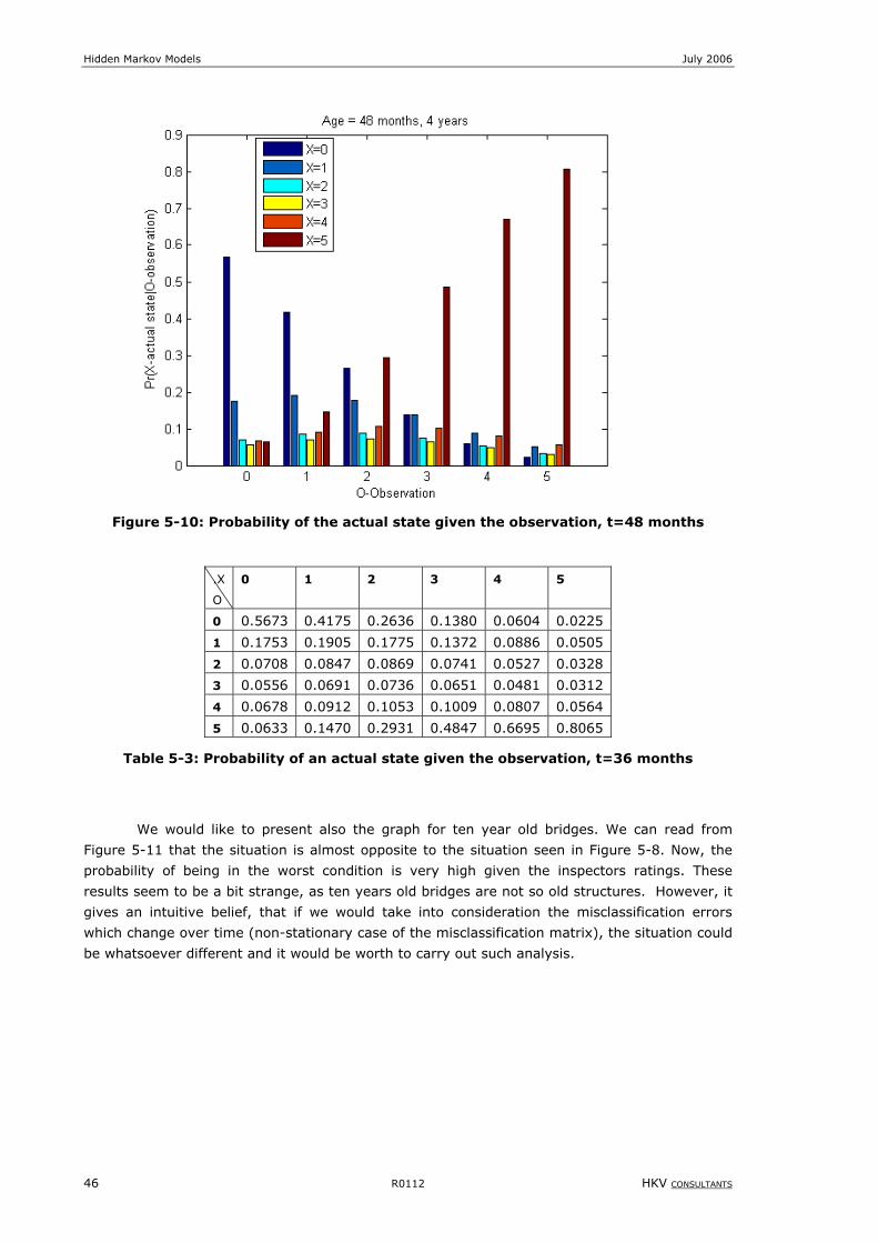
Hidden Markov Models July 2006
46 R0112 HKV CONSULTANTS
Figure 5-10: Probability of the actual state given the observation, t=48 months
.X
O
0 1 2 3 4 5
0 0.5673 0.4175 0.2636 0.1380 0.0604 0.0225
1 0.1753 0.1905 0.1775 0.1372 0.0886 0.0505
2 0.0708 0.0847 0.0869 0.0741 0.0527 0.0328
3 0.0556 0.0691 0.0736 0.0651 0.0481 0.0312
4 0.0678 0.0912 0.1053 0.1009 0.0807 0.0564
5 0.0633 0.1470 0.2931 0.4847 0.6695 0.8065
Table 5-3: Probability of an actual state given the observation, t=36 months
We would like to present also the graph for ten year old bridges. We can read from
Figure 5-11 that the situation is almost opposite to the situation seen in Figure 5-8. Now, the
probability of being in the worst condition is very high given the inspectors ratings. These
results seem to be a bit strange, as ten years old bridges are not so old structures. However, it
gives an intuitive belief, that if we would take into consideration the misclassification errors
which change over time (non-stationary case of the misclassification matrix), the situation could
be whatsoever different and it would be worth to carry out such analysis.
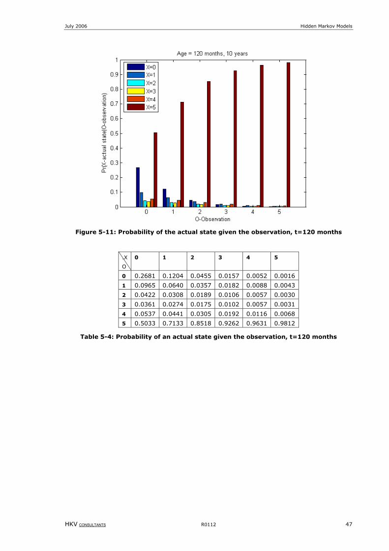
July 2006 Hidden Markov Models
HKV CONSULTANTS R0112 47
Figure 5-11: Probability of the actual state given the observation, t=120 months
.X
O
0 1 2 3 4 5
0 0.2681 0.1204 0.0455 0.0157 0.0052 0.0016
1 0.0965 0.0640 0.0357 0.0182 0.0088 0.0043
2 0.0422 0.0308 0.0189 0.0106 0.0057 0.0030
3 0.0361 0.0274 0.0175 0.0102 0.0057 0.0031
4 0.0537 0.0441 0.0305 0.0192 0.0116 0.0068
5 0.5033 0.7133 0.8518 0.9262 0.9631 0.9812
Table 5-4: Probability of an actual state given the observation, t=120 months


July 2006 Hidden Markov Models
HKV CONSULTANTS R0112 49
6 First time to reach a failure
In this chapter we will try to answer the question: how long it will take for a process to
reach state j from state i for the first time. The time required before the state will move from i
to j for the first time is referred to as the first passage time. However, the most interesting
aspect for us is to get to know how fast a bridge goes from the perfect condition ‘0’ to the very
bad condition ‘5’ (failure). This information can help a decision-maker to fix an optimal time to
carry out the inspections. Properly scheduled inspections can allow for minimizing the cost of
maintenance and in the same time for keeping the bridges safe for their users.
We can pose the question about the average time of reaching the worst state, assuming
that the process starts from the perfect condition. We will compare the mean time of reaching
state ‘5’ from state ‘0’ for perfect inspections and for imperfect inspections. Moreover, we are
highly interested in finding how the mean time of reaching state ‘5’ changes when the time
interval of inspections changes.
6.1 Perfect inspections
At the beginning, we consider a situation where the conditions of the bridges indicate
the real states of the bridges. In other words, we assume that the inspectors made no error in
the assessment of the bridges’ conditions. So the process can go only forward. We do so, in
order to compare how the situation will change when we introduce inspections with possible
errors.
For a Markov process we define:
{ }jXsT sj =≥= :1inf
which is the first time that the process sX visits the state j, [3]. That is, sT j = if and only if
jXk ≠ for k=1,2,…,s-1 and jX s = . We define the probability density function ijf as:
(6-1) ),...,,,Pr()Pr()( 01210 iXjXjXjXjXiXsTsf sssjij =≠≠≠===== −−
The probability density function )(sf ij can be calculated recursively via:
(6-2)
=
>−⋅= ∑
≠
1
1)1()(
sifP
sifsfPsf
ij
n
jkkjik
ij
To see this, we have for 2≥s :
(6-3) ∑≠
− ===≠≠==jk
ssij iXjXjXjXkXsf ),,...,,Pr()( 0121
∑≠
− ==≠≠⋅===jk
ss kXjXjXjXiXkX ),,...,Pr()Pr( 11201
But, by the Markov property and stationarity, it follows that:
∑∑≠
−≠
−− ⋅===≠≠≠⋅===jk
skjikjk
ssij fPkXjXjXjXjXiXkXsf )1(0122101 ),,...,,Pr()Pr()(
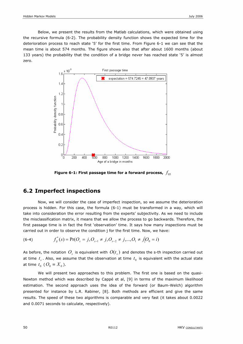
Hidden Markov Models July 2006
50 R0112 HKV CONSULTANTS
Below, we present the results from the Matlab calculations, which were obtained using
the recursive formula (6-2). The probability density function shows the expected time for the
deterioration process to reach state ‘5’ for the first time. From Figure 6-1 we can see that the
mean time is about 574 months. The figure shows also that after about 1600 months (about
133 years) the probability that the condition of a bridge never has reached state ‘5’ is almost
zero.
Figure 6-1: First passage time for a forward process, 05f
6.2 Imperfect inspections
Now, we will consider the case of imperfect inspection, so we assume the deterioration
process is hidden. For this case, the formula (6-1) must be transformed in a way, which will
take into consideration the error resulting from the experts’ subjectivity. As we need to include
the misclassification matrix, it means that we allow the process to go backwards. Therefore, the
first passage time is in fact the first ‘observation’ time. It says how many inspections must be
carried out in order to observe the condition j for the first time. Now, we have:
(6-4) ),...,,,Pr()( 0121* iOjOjOjOjOsf sssij =≠≠≠== −−
As before, the notation sO is equivalent with )( stO and denotes the s-th inspection carried out
at time st . Also, we assume that the observation at time 0t is equivalent with the actual state
at time 0t ( 00 XO ≡ ).
We will present two approaches to this problem. The first one is based on the quasi-
Newton method which was described by Cappé et al, [9] in terms of the maximum likelihood
estimation. The second approach uses the idea of the forward (or Baum-Welch) algorithm
presented for instance by L.R. Rabiner, [8]. Both methods are efficient and give the same
results. The speed of these two algorithms is comparable and very fast (it takes about 0.0022
and 0.0071 seconds to calculate, respectively).
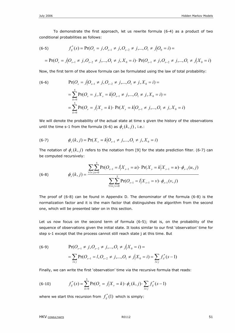
July 2006 Hidden Markov Models
HKV CONSULTANTS R0112 51
To demonstrate the first approach, let us rewrite formula (6-4) as a product of two
conditional probabilities as follows:
(6-5) ==≠≠≠== −− ),...,,,Pr()( 0121* iOjOjOjOjOsf sssij
),...,,Pr(),,...,,Pr( 01210121 iXjOjOjOiXjOjOjOjO sssss =≠≠≠⋅=≠≠≠== −−−−
Now, the first term of the above formula can be formulated using the law of total probability:
(6-6) ==≠≠≠= −− ),,...,,Pr( 0121 iXjOjOjOjO sss
==≠≠=== ∑=
−
5
0011 ),,...,,Pr(
ksss iXjOjOkXjO
),,...,Pr()Pr( 011
5
0iXjOjOkXkXjO ss
kss =≠≠=⋅=== −
=∑
We will denote the probability of the actual state at time s given the history of the observations
until the time s-1 from the formula (6-6) as ),( jksφ , i.e.:
(6-7) ),,...,Pr(),( 011 iXjOjOkXjk sss =≠≠== −φ
The notation of ),( jksφ refers to the notation from [9] for the state prediction filter. (6-7) can
be computed recursively:
(6-8)
∑∑
∑∑
≠∀−
=−−
−≠∀
−=
−−
⋅==
⋅==⋅===
jls
vss
sjl
ssu
ss
s
jvvXlO
juuXkXuXlOjk
),()Pr(
),()Pr()Pr(),(
1
5
011
11
5
011
φ
φφ
The proof of (6-8) can be found in Appendix D. The denominator of the formula (6-8) is the
normalization factor and it is the main factor that distinguishes the algorithm from the second
one, which will be presented later on in this section.
Let us now focus on the second term of formula (6-5); that is, on the probability of the
sequence of observations given the initial state. It looks similar to our first ‘observation’ time for
step s-1 except that the process cannot still reach state j at this time. But
(6-9) ==≠≠≠ −− ),...,,Pr( 0121 iXjOjOjO ss
∑∑≠≠
−− −==≠≠==jl
iljl
ss sfiXjOjOlO )1(),...,,Pr( *0121
Finally, we can write the first ‘observation’ time via the recursive formula that reads:
(6-10) ∑ ∑= ≠
−⋅⋅===5
0
** )1(),()Pr()(k jl
ijsssij sfjkkXjOsf φ
where we start this recursion from )1(*ijf which is simply:
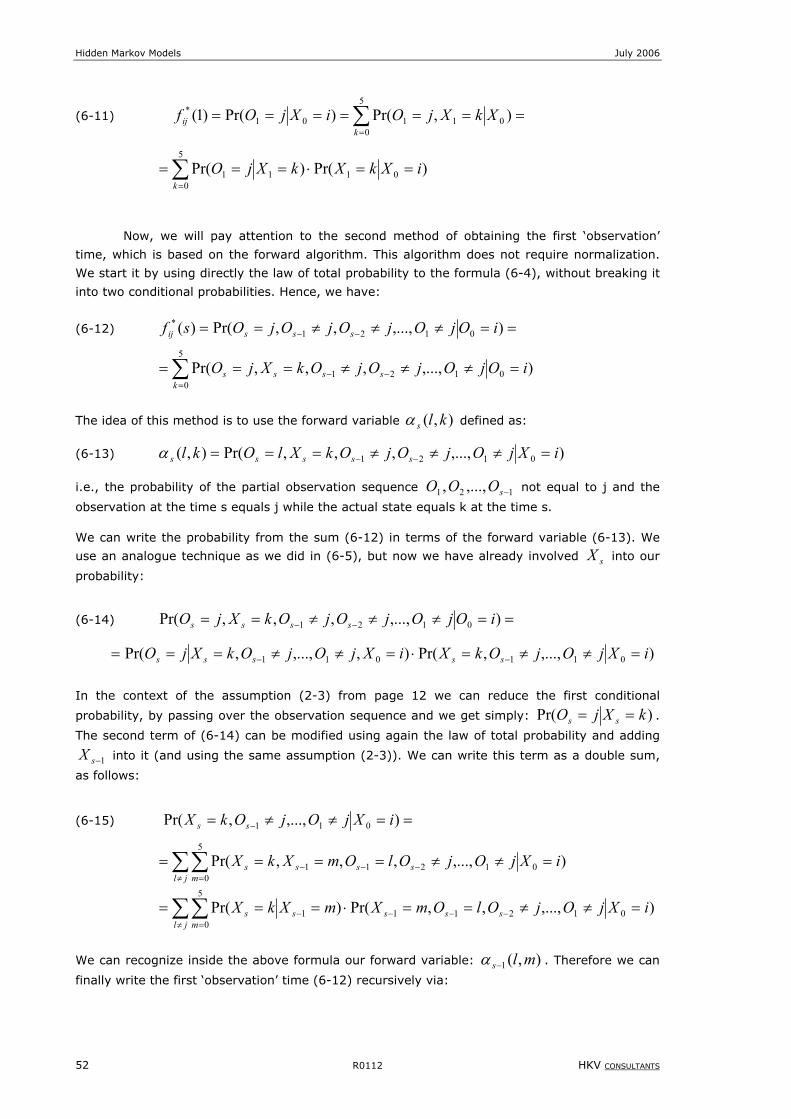
Hidden Markov Models July 2006
52 R0112 HKV CONSULTANTS
(6-11) ∑=
=======5
001101
* ),Pr()Pr()1(k
ij XkXjOiXjOf
∑=
==⋅===5
00111 )Pr()Pr(
kiXkXkXjO
Now, we will pay attention to the second method of obtaining the first ‘observation’
time, which is based on the forward algorithm. This algorithm does not require normalization.
We start it by using directly the law of total probability to the formula (6-4), without breaking it
into two conditional probabilities. Hence, we have:
(6-12) ==≠≠≠== −− ),...,,,Pr()( 0121* iOjOjOjOjOsf sssij
∑=
−− =≠≠≠===5
00121 ),...,,,,Pr(
kssss iOjOjOjOkXjO
The idea of this method is to use the forward variable ),( klsα defined as:
(6-13) ),...,,,,Pr(),( 0121 iXjOjOjOkXlOkl sssss =≠≠≠=== −−α
i.e., the probability of the partial observation sequence 121 ,...,, −sOOO not equal to j and the
observation at the time s equals j while the actual state equals k at the time s.
We can write the probability from the sum (6-12) in terms of the forward variable (6-13). We
use an analogue technique as we did in (6-5), but now we have already involved sX into our
probability:
(6-14) ==≠≠≠== −− ),...,,,,Pr( 0121 iOjOjOjOkXjO ssss
= ),...,,Pr(),,...,,Pr( 011011 iXjOjOkXiXjOjOkXjO sssss =≠≠=⋅=≠≠== −−
In the context of the assumption (2-3) from page 12 we can reduce the first conditional
probability, by passing over the observation sequence and we get simply: )Pr( kXjO ss == .
The second term of (6-14) can be modified using again the law of total probability and adding
1−sX into it (and using the same assumption (2-3)). We can write this term as a double sum,
as follows:
(6-15) ==≠≠= − ),...,,Pr( 011 iXjOjOkX ss
∑∑≠ =
−−− =≠≠====jl m
ssss iXjOjOlOmXkX5
001211 ),...,,,,Pr(
),...,,,Pr()Pr( 01211
5
01 iXjOjOlOmXmXkX sss
jl mss =≠≠==⋅=== −−−
≠ =−∑∑
We can recognize inside the above formula our forward variable: ),(1 mls−α . Therefore we can
finally write the first ‘observation’ time (6-12) recursively via:
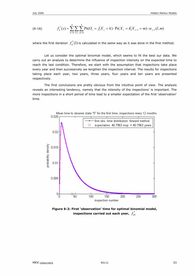
July 2006 Hidden Markov Models
HKV CONSULTANTS R0112 53
(6-16) ∑∑∑= ≠
−=
− ⋅==⋅===5
01
5
01
* ),()Pr()Pr()(k jl
sm
ssssij mlmXkXkXjOsf α
where the first iteration )1(*ijf is calculated in the same way as it was done in the first method.
Let us consider the optimal binomial model, which seems to fit the best our data. We
carry out an analysis to determine the influence of inspection intensity on the expected time to
reach the last condition. Therefore, we start with the assumption that inspections take place
every year and then successively we lengthen the inspection interval. The results for inspections
taking place each year, two years, three years, four years and ten years are presented
respectively.
The first conclusions are pretty obvious from the intuitive point of view. The analysis
reveals an interesting tendency, namely that the intensity of the inspections’ is important. The
more inspections in a short period of time lead to a smaller expectation of the first ‘observation’
time.
Figure 6-2: First ‘observation’ time for optimal binomial model,
inspections carried out each year, *05f
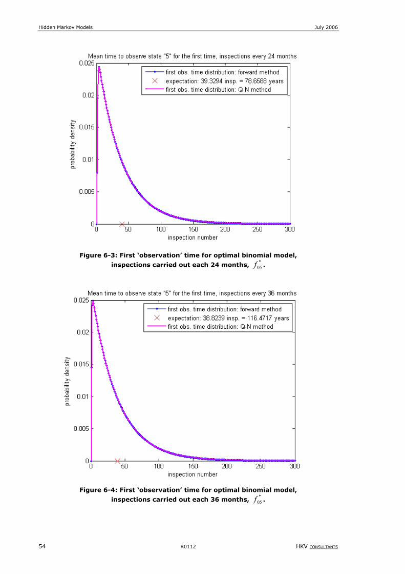
Hidden Markov Models July 2006
54 R0112 HKV CONSULTANTS
Figure 6-3: First ‘observation’ time for optimal binomial model,
inspections carried out each 24 months, *05f .
Figure 6-4: First ‘observation’ time for optimal binomial model,
inspections carried out each 36 months, *05f .
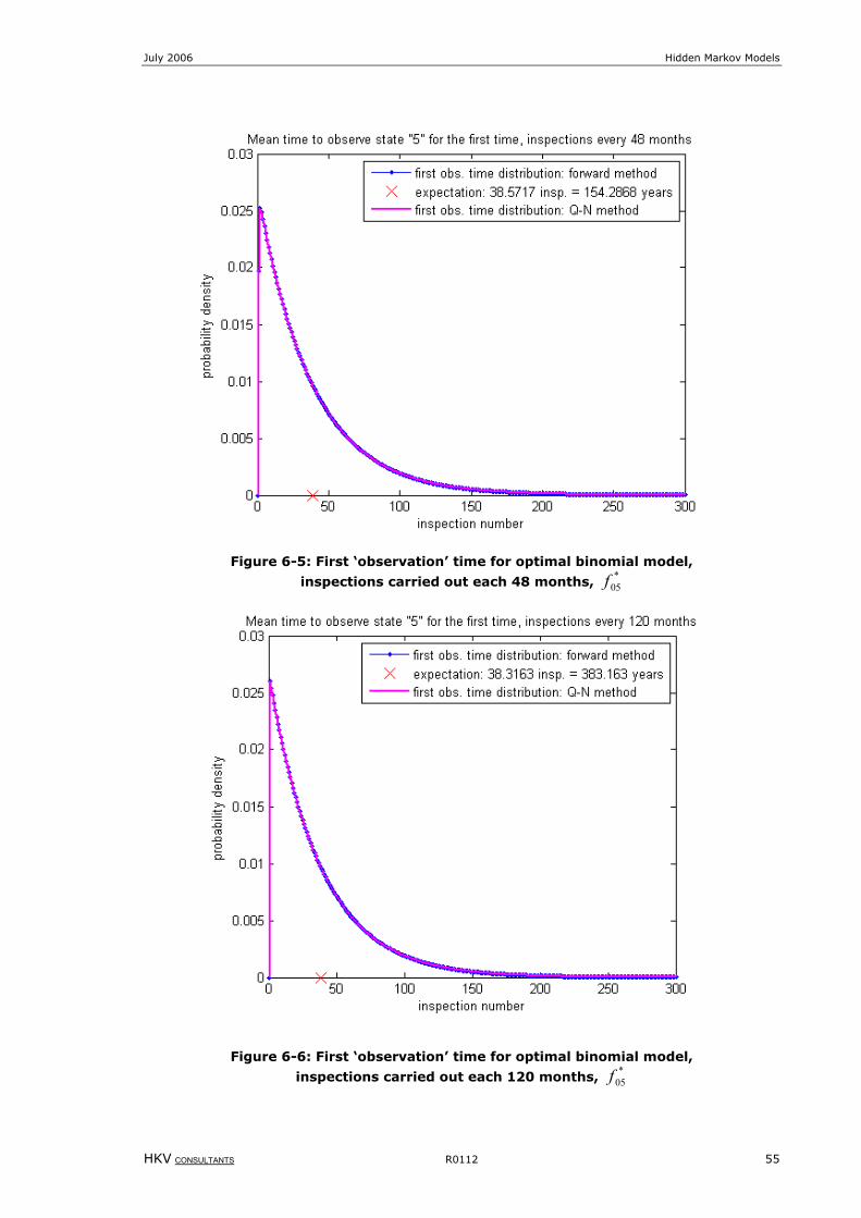
July 2006 Hidden Markov Models
HKV CONSULTANTS R0112 55
Figure 6-5: First ‘observation’ time for optimal binomial model,
inspections carried out each 48 months, *05f
Figure 6-6: First ‘observation’ time for optimal binomial model,
inspections carried out each 120 months, *05f
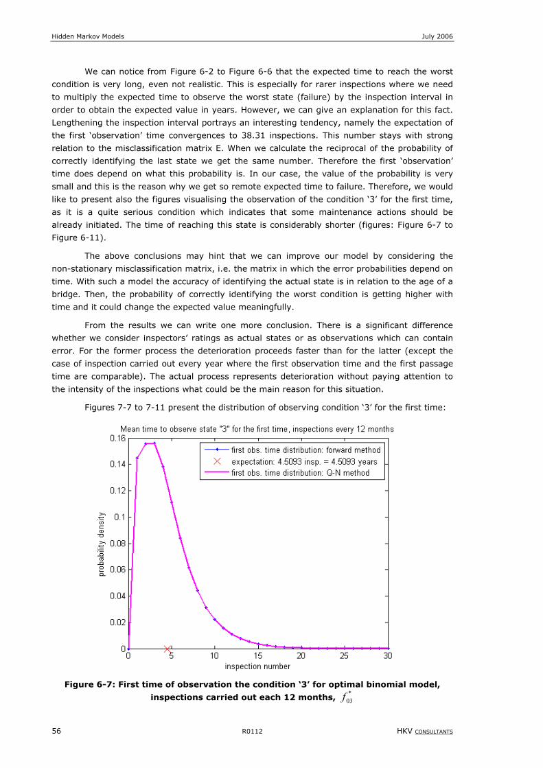
Hidden Markov Models July 2006
56 R0112 HKV CONSULTANTS
We can notice from Figure 6-2 to Figure 6-6 that the expected time to reach the worst
condition is very long, even not realistic. This is especially for rarer inspections where we need
to multiply the expected time to observe the worst state (failure) by the inspection interval in
order to obtain the expected value in years. However, we can give an explanation for this fact.
Lengthening the inspection interval portrays an interesting tendency, namely the expectation of
the first ‘observation’ time convergences to 38.31 inspections. This number stays with strong
relation to the misclassification matrix E. When we calculate the reciprocal of the probability of
correctly identifying the last state we get the same number. Therefore the first ‘observation’
time does depend on what this probability is. In our case, the value of the probability is very
small and this is the reason why we get so remote expected time to failure. Therefore, we would
like to present also the figures visualising the observation of the condition ‘3’ for the first time,
as it is a quite serious condition which indicates that some maintenance actions should be
already initiated. The time of reaching this state is considerably shorter (figures: Figure 6-7 to
Figure 6-11).
The above conclusions may hint that we can improve our model by considering the
non-stationary misclassification matrix, i.e. the matrix in which the error probabilities depend on
time. With such a model the accuracy of identifying the actual state is in relation to the age of a
bridge. Then, the probability of correctly identifying the worst condition is getting higher with
time and it could change the expected value meaningfully.
From the results we can write one more conclusion. There is a significant difference
whether we consider inspectors’ ratings as actual states or as observations which can contain
error. For the former process the deterioration proceeds faster than for the latter (except the
case of inspection carried out every year where the first observation time and the first passage
time are comparable). The actual process represents deterioration without paying attention to
the intensity of the inspections what could be the main reason for this situation.
Figures 7-7 to 7-11 present the distribution of observing condition ‘3’ for the first time:
Figure 6-7: First time of observation the condition ‘3’ for optimal binomial model,
inspections carried out each 12 months, *03f
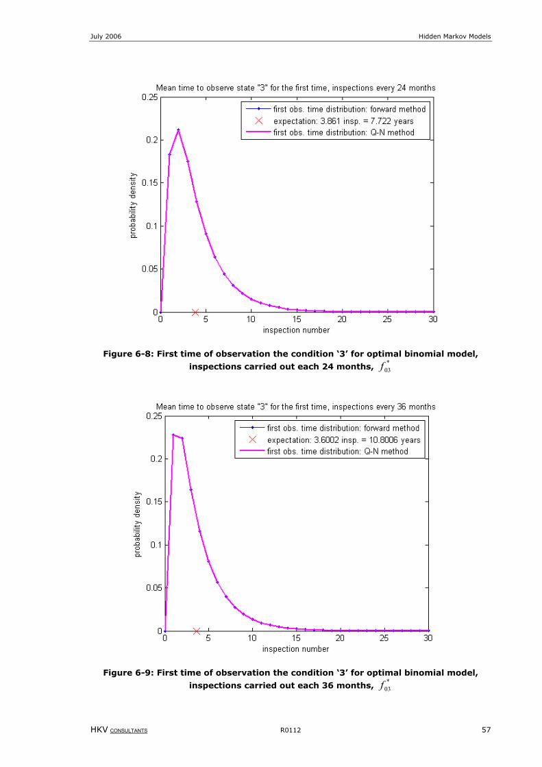
July 2006 Hidden Markov Models
HKV CONSULTANTS R0112 57
Figure 6-8: First time of observation the condition ‘3’ for optimal binomial model,
inspections carried out each 24 months, *03f
Figure 6-9: First time of observation the condition ‘3’ for optimal binomial model,
inspections carried out each 36 months, *03f
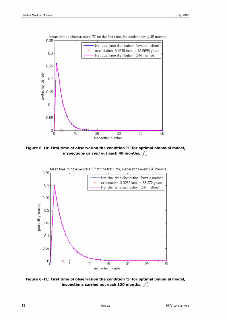
Hidden Markov Models July 2006
58 R0112 HKV CONSULTANTS
Figure 6-10: First time of observation the condition ‘3’ for optimal binomial model,
inspections carried out each 48 months, *03f
Figure 6-11: First time of observation the condition ‘3’ for optimal binomial model,
inspections carried out each 120 months, *03f
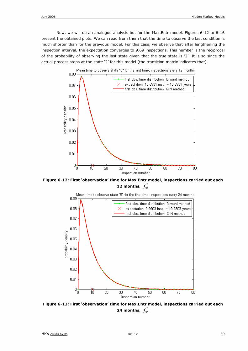
July 2006 Hidden Markov Models
HKV CONSULTANTS R0112 59
Now, we will do an analogue analysis but for the Max.Entr model. Figures 6-12 to 6-16
present the obtained plots. We can read from them that the time to observe the last condition is
much shorter than for the previous model. For this case, we observe that after lengthening the
inspection interval, the expectation converges to 9.69 inspections. This number is the reciprocal
of the probability of observing the last state given that the true state is ‘2’. It is so since the
actual process stops at the state ‘2’ for this model (the transition matrix indicates that).
Figure 6-12: First ‘observation’ time for Max.Entr model, inspections carried out each
12 months, *05f
Figure 6-13: First ‘observation’ time for Max.Entr model, inspections carried out each
24 months, *05f
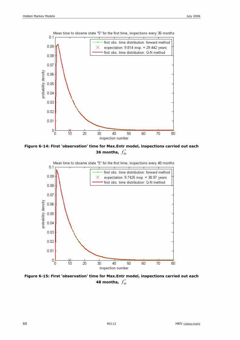
Hidden Markov Models July 2006
60 R0112 HKV CONSULTANTS
Figure 6-14: First ‘observation’ time for Max.Entr model, inspections carried out each
36 months, *05f
Figure 6-15: First ‘observation’ time for Max.Entr model, inspections carried out each
48 months, *05f
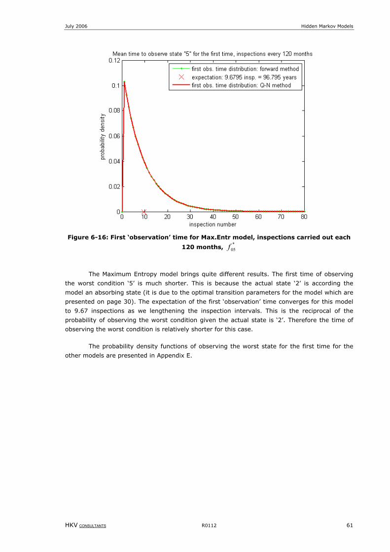
July 2006 Hidden Markov Models
HKV CONSULTANTS R0112 61
Figure 6-16: First ‘observation’ time for Max.Entr model, inspections carried out each
120 months, *05f
The Maximum Entropy model brings quite different results. The first time of observing
the worst condition ‘5’ is much shorter. This is because the actual state ‘2’ is according the
model an absorbing state (it is due to the optimal transition parameters for the model which are
presented on page 30). The expectation of the first ‘observation’ time converges for this model
to 9.67 inspections as we lengthening the inspection intervals. This is the reciprocal of the
probability of observing the worst condition given the actual state is ‘2’. Therefore the time of
observing the worst condition is relatively shorter for this case.
The probability density functions of observing the worst state for the first time for the
other models are presented in Appendix E.

July 2006 Hidden Markov Models
HKV CONSULTANTS R0112 63
7 Conclusions
The thesis concentrates on the analysis leading to developing a deterioration model for
the bridges in the Netherlands. The model was based on the results from visual inspections that
are collected in the database called ‘DISK’. The bridges are rated on the discrete scale from ‘0’
to ‘5’ (in fact from ‘0’ to ‘6,’ but due to the small amount of data we have decided to merge the
last two states together), where ‘0’ means perfect condition and ‘5’ means very bad condition
(failure). Therefore we have used the Markovian model as a mathematical tool. Since the
inspections are carried out only visually, a lot of factors can influence the expert opinions about
the bridge conditions. Hence, the main aim was to take the subjectivity of the inspectors into
account. In order to do that, we introduced the Hidden Markov Model where the observation is a
probabilistic function of the state. In this model, the actual process is not observable directly (it
is hidden), but can only be determined through the sequence of observations.
The Markov property indicates that given the present the history of the process is not
important and the future prediction of the state depends only on the present state. However, it
concerns the hidden process not the observable one. The Markov property does not hold for the
observable process, but only for the actual process. We assume independence of the inspections
given the values of the real deterioration process.
The most important challenge during this work was to derive the formula for the
likelihood functions of the data that would take into account the parameters of the model. We
have had two types of the parameters, namely the transition and the misclassification
parameters. The transition parameters describe the probabilities of moving to the next states
for the actual deterioration process. The misclassification parameters model the probabilities of
inspector errors. Both types of parameters create matrices: the transition and misclassification
matrix, respectively.
Literature describes a few approaches for fitting the transition and misclassification
matrix. We decided to implement the method proposed by Jackson in [1]. Although the method
is not given via recursive formulation, it allows for writing the likelihood function in terms of the
matrices product and therefore makes the implementation passable. Unfortunately, the
optimization algorithm to implement the maximum likelihood method for estimating the
parameters is not a perfect method. It can happen that the solution is only a local maximum. It
is difficult to judge whether we obtain a global or local solution and there is no algorithm which
could confirm that. A possible way to verify it is to start the maximization scheme with various
initial guesses and to make sure that it leads to the same values of the optimal parameters. If
this is the case, we can suppose that we have indeed found the global maximum. Another
approach is using global optimization methods (such as genetic algorithms).
Taking the inspectors’ subjectivity into consideration allows for the possibilities of seeing
a better condition for the bridge than it was on the previous inspections. In other words, we
needed to accept that the condition can improve. However, we excluded transitions that could
indicate maintenance from the data. Therefore, we assumed that the improvements in the
conditions are only due to expert-judgment errors. It reflects the way of choosing both
matrices: the transition and the misclassification matrix. The transition matrix does not allow
the process to go backward. It only allows a bridge to move one condition forward in one unit of
time (month). But the choice of the misclassification matrix needed to be adequate. Since we
had to take into account all possible errors between the observations and the actual states, the
misclassification matrix had to be fully filled.
Hidden Markov Models July 2006
64 R0112 HKV CONSULTANTS
We have introduced a few types of misclassification matrices which can describe the
inspectors’ errors. With the use of the optimization algorithm the optimal one was found, i.e.
the one with the maximum likelihood value, together with the transition matrix. The
probabilities of error were higher for the better conditions (from ‘0’ to ‘2’) in the
misclassification matrix. This means that the inspectors are more likely to rate a condition of a
bridge as satisfactory and therefore they make more mistakes within this part of the scale.
Imposing the expected value of the observed state equal to the actual state, a different
type of misclassification matrix was built, namely the maximum entropy matrix. In this way, we
obtained the probability distribution for the misclassification errors with maximum entropy given
a fixed mean (i.e. with the minimum extra information). Also, we built the misclassification
matrix using the binomial distribution with fixed mean in order to compare those two matrices
in terms of the amount of additional information that they add. The analysis has shown that
with such misclassification matrices, the optimal transition parameters became meaningful
different. In these cases, transitions to the worse states were rather due to the error of the
inspectors than due to the deterioration progress. The reason for this result was connected with
the fact that these distributions put higher probabilities of error for the worse observations
(form ‘3’ to ‘5’) in the misclassification matrix.
Since, the fully filled misclassification matrix assumed that the inspection error can span
the whole range, it can be too uncertain. Therefore, other models were also considered, where
only some of the places in the misclassification matrix were not equal to zero. It was connected
with removing all transitions from the data which result in zero values for the likelihood
function. The binomial model with such an incomplete misclassification matrix (‘Misclassification
matrix 2’) has given quite nice results. All the parameters in this model differed from zero.
However, the tendency from the previous models was kept, namely the probabilities of error
stayed high for the better conditions. It indicates that the probability of correctly identifying the
worst state was almost zero. This fact had a big influence on the further analysis of the time of
first observing the worst state. We have also considered a model with a misclassification matrix
which allows the error to be of the difference of one state at the most (‘Misclassification matrix
1’). This matrix turned out to be close to the one for the perfect inspection. In other words, for
this case, the optimal parameters indicate that the inspectors are almost perfect experts.
The misclassification matrix that comes from the maximum entropy method was
generated according to some reasonable constraints (the mean was known and equal to the
actual state). However, for this case the probabilities of correctly identifying the worse states
were getting smaller, which is not the desired tendency. For the optimal binomial model, those
probabilities were even smaller. It makes those models to be defective. The misclassification
matrix resulting from the binomial model with a fixed mean seems to be much better in this
respect. Therefore it is worth to pay attention to this matrix in the future research.
Furthermore, it does not have to be a fully filled matrix. A partially filled misclassification
matrix, which is generated according to a binomial distribution with a fixed mean could be also
a good choice.
For the various misclassification models, we have illustrated the expectation for both the
actual state and the observed state for various models. They gave different results, as the
expected condition involved the probabilities of error. The expectation of the actual states
converged to the worst state, while the expectation of the observation never reached this level.
Moreover, the latter expectation was close to the line which indicated the average condition of
bridges in a particular age from the data. However, it differed depending on the model.

July 2006 Hidden Markov Models
HKV CONSULTANTS R0112 65
Using Bayes’ rule, we were able to calculate the probability of the actual state given the
observed state. From this probability, we were able to read what the most probable actual state
of a bridge is when an inspector gives it a particular rating.
In the last chapter we have presented the idea of the mean time to reach the worst
state (first passage time) and its extension to the mean time to observe the worst state (first
‘observation’ time). They were described in terms of the probability density functions. The
recursive formula for the density function for perfect inspection is not complicated and can be
found in the literature. However, the first ‘observation’ time requires an algorithm that is more
complex. The complexity results mainly from the fact that the sequence of observations does
not have the Markov property as the hidden process has. Two approaches for this problem were
presented which give the same results. Furthermore, the probability density functions of the
first ‘observation’ times were calculated for various inspection intervals. The analysis reveals
that the intensity of the inspections has a large impact on the mean time to observe a failure.
The more often the inspections take place the shorter the mean time to observe the worst
condition is. From the results, it is clear that the mean time to observe the failure is connected
with the misclassification probability, precisely with the probability of correctly identifying the
worst state (for the optimal binomial model). The mean time converges to the reciprocal of this
probability. Therefore the higher this probability is, the shorter the mean time to failure.
Recommendation for future research:
In our analysis we assumed both the transition matrix and the misclassification matrix
to be state-dependent and time-independent (stationary). However, taking the non-stationary
model, especially the non-stationary misclassification matrix, could improve the results in great
deal and it would be interesting to make such analysis in future research.
It will be useful to test the inspectors to have better knowledge how much their
assessments could differ from the real states. In other words, what is the biggest error they can
make. Then it would be clearer how to fill the misclassification matrix and whether it must be
fully filled or not.
We implemented the likelihood function based on one method proposed by Jackson, [1].
The other mentioned models could be implemented and the results compared.
Since the transitions that could indicate maintenance were removed from the data, the
model did not take them into account. Including them into the model would be an interesting
challenge.
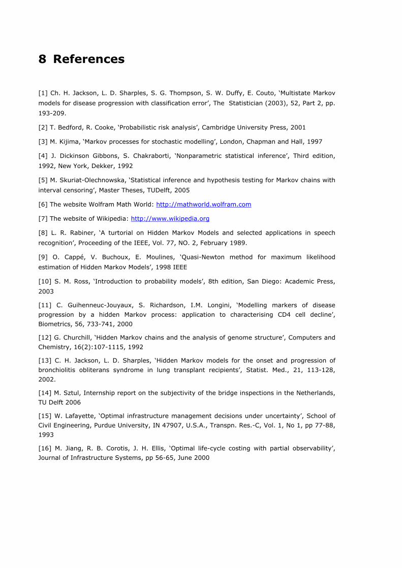
8 References
[1] Ch. H. Jackson, L. D. Sharples, S. G. Thompson, S. W. Duffy, E. Couto, ‘Multistate Markov
models for disease progression with classification error’, The Statistician (2003), 52, Part 2, pp.
193-209.
[2] T. Bedford, R. Cooke, ‘Probabilistic risk analysis’, Cambridge University Press, 2001
[3] M. Kijima, ‘Markov processes for stochastic modelling’, London, Chapman and Hall, 1997
[4] J. Dickinson Gibbons, S. Chakraborti, ‘Nonparametric statistical inference’, Third edition,
1992, New York, Dekker, 1992
[5] M. Skuriat-Olechnowska, ‘Statistical inference and hypothesis testing for Markov chains with
interval censoring’, Master Theses, TUDelft, 2005
[6] The website Wolfram Math World: http://mathworld.wolfram.com
[7] The website of Wikipedia: http://www.wikipedia.org
[8] L. R. Rabiner, ‘A turtorial on Hidden Markov Models and selected applications in speech
recognition’, Proceeding of the IEEE, Vol. 77, NO. 2, February 1989.
[9] O. Cappé, V. Buchoux, E. Moulines, ‘Quasi-Newton method for maximum likelihood
estimation of Hidden Markov Models’, 1998 IEEE
[10] S. M. Ross, ‘Introduction to probability models’, 8th edition, San Diego: Academic Press,
2003
[11] C. Guihenneuc-Jouyaux, S. Richardson, I.M. Longini, ‘Modelling markers of disease
progression by a hidden Markov process: application to characterising CD4 cell decline’,
Biometrics, 56, 733-741, 2000
[12] G. Churchill, ‘Hidden Markov chains and the analysis of genome structure’, Computers and
Chemistry, 16(2):107-1115, 1992
[13] C. H. Jackson, L. D. Sharples, ‘Hidden Markov models for the onset and progression of
bronchiolitis obliterans syndrome in lung transplant recipients’, Statist. Med., 21, 113-128,
2002.
[14] M. Sztul, Internship report on the subjectivity of the bridge inspections in the Netherlands,
TU Delft 2006
[15] W. Lafayette, ‘Optimal infrastructure management decisions under uncertainty’, School of
Civil Engineering, Purdue University, IN 47907, U.S.A., Transpn. Res.-C, Vol. 1, No 1, pp 77-88,
1993
[16] M. Jiang, R. B. Corotis, J. H. Ellis, ‘Optimal life-cycle costing with partial observability’,
Journal of Infrastructure Systems, pp 56-65, June 2000

Appendices


July 2006 Hidden Markov Models
HKV CONSULTANTS R0112.20 A-1
Appendix A: Specific bridges from the data
We present all the cases from the data that indicate the value zero of the likelihood function,
when the misclassification matrix is of the first type.
Bridge
index Age of a bridge
[in months]
Age of a bridge
[in months]
Condition
state
Condition
state
Year of
construction
127 198 213 1 3 1976
127 213 283 3 0 1976
410 307 318 2 5 1967
410 318 325 5 0 1967
410 325 390 0 3 1967
410 390 414 3 3 1967
410 414 454 3 3 1967
417 251 382 4 3 1970
417 382 411 3 1 1970
454 214 302 1 3 1970
454 302 310 3 5 1970
454 310 364 5 2 1970
779 716 727 4 1 1933
779 727 764 1 3 1933
800 234 262 4 1 1973
848 292 380 5 2 1966
856 665 694 4 3 1937
856 694 753 3 1 1937
932 437 481 5 1 1956
939 0 53 0 5 1988
939 53 56 5 4 1988
939 56 82 4 2 1988
1401 253 268 4 1 1970
1401 268 315 1 2 1970
1424 149 215 5 3 1980
1424 215 294 3 2 1980
1449 616 666 3 3 1939
1449 666 719 3 0 1939
1622 358 419 2 4 1957
1622 419 459 4 4 1957
1622 459 515 4 3 1957
1622 515 546 3 1 1957
1698 87 119 5 2 1985
1765 563 601 4 1 1940
1765 601 659 1 3 1940
1765 659 713 3 2 1940
1766 556 589 5 2 1941
1766 589 642 2 2 1941
1766 642 701 2 3 1941
1808 239 279 1 5 1970

Hidden Markov Models July 2006
HKV CONSULTANTS R0112.20 A-2
1808 279 390 5 1 1970
1809 239 279 1 4 1970
1809 279 390 4 1 1970
1901 446 453 3 0 1955
1901 453 558 0 3 1955
2029 220 229 1 1 1969
2029 229 291 1 4 1969
2029 291 410 4 1 1969
2052 279 339 2 5 1965
2052 339 460 5 2 1965
2131 297 353 2 5 1963
2131 353 476 5 2 1963
2132 297 353 2 5 1963
2132 353 476 5 2 1963
2147 250 305 1 5 1967
2147 305 428 5 2 1967
2198 198 255 1 5 1972
2198 255 368 5 2 1972
2240 381 395 3 3 1961
2240 395 432 3 0 1961
2257 346 357 3 0 1963
2260 238 249 3 0 1972
2260 249 369 0 2 1972
2262 658 669 3 0 1937
2262 669 789 0 3 1937
2285 395 405 3 0 1959
2285 405 460 0 3 1959
Table A-1: Specific structures from the data

July 2006 Hidden Markov Models
HKV CONSULTANTS R0112.20 B-1
Appendix B: Proof of the formula for the likelihood (4-3)
We shall prove that the likelihood of the form (4-2):
===== ),...,,Pr()( 2211 mim
iii jOjOjOL θ
),...,Pr(),...,,...,Pr( 111111 mim
im
im
im
im
i lXlXlXlXjOjO ==⋅===== ∑
(where the sum is taken over all possible paths of the actual states ml ), can be expressed by
the formula (4-3):
∑∑==
⋅====⋅====5
01122222211
5
01111
2
)Pr()Pr()Pr()Pr()(l
iiiii
l
iii lXlXlXjOlXlXjOL
l
θ
∑∑=
−−=
====⋅⋅====5
011
5
022333333 )Pr()Pr(...)Pr()Pr(
3 mlm
imm
imm
imm
im
l
iiii lXlXlXjOlXlXlXjO
Proof:
To make the formulas easier to write down, we will shorten the notation as follows:
),...,(),...,( 111 mmim
i OOjOjO ≡== and ),...,(),...,( 111 mmim
i XXlXlX ≡== .
We will start with the equation (4-3) and will finish with the form corresponding to the equation
(4-4). Using the necessary assumptions, we have:
∑∑ ∑∀ ∀ ∀
==1 2
),...,,...,,Pr(...),...,,Pr( 12121X X X
mmmm
XXOOOOOO
∑∑ ∑∀ ∀ ∀
=⋅=1 2
),Pr(),,,...,,Pr(... 111122X X X
mmm
XOXOXOXO
∑ ∑ ∑∀ ∀ ∀
=⋅=1 2
),,...,,Pr(...),Pr( 12211X X X
mmm
XXOXOXO
∑ ∑ ∑∀ ∀ ∀
=⋅⋅=1 2
)Pr(),,,...,,Pr(
...)Pr()Pr(1
122111
X X X
mm
mX
XXOXOXXO
∑ ∑ ∑∀ ∀ ∀
⋅⋅⋅=
1 2)Pr(
),,...,Pr(),,...,,...,Pr(...)Pr()Pr(
1
12122111
X X X
mmm
mX
XXXXXXOOXXO
Furthermore:
)Pr(....)Pr(),...,Pr(....),...,Pr(),...,,...,Pr( 2212112 XOXOXXOXXOXXOO mmmmmmm ⋅⋅=⋅⋅=
Therefore, to finish the proof we need to show that:

Hidden Markov Models July 2006
B-2 R0112.20 HKV CONSULTANTS
)Pr(...)Pr()Pr()Pr(
),,...,Pr(12211
1
12 XXXXXXX
XXXmmmm
m ⋅⋅⋅= −−−
But we have:
=⋅
= −−
)Pr(),,...,Pr(),,...,Pr(
)Pr(),,...,Pr(
1
121121
1
12
XXXXXXXX
XXXX mmmm
==⋅⋅
= −−−− ...)Pr(
),...,Pr(),,...,Pr(),,...,Pr(
1
121221121
XXXXXXXXXXX mmmmm
)Pr()Pr()Pr(....),,...,Pr(
1
112121
XXXXXXXX mm ⋅⋅⋅
= −
Now, using the Markov property we get the final result.

July 2006 Hidden Markov Models
HKV CONSULTANTS R0112.20 C-1
Appendix C: The extreme cases from the new data
Below, we present some results of ratings the bridges from the modified data. These
cases indicate how fast the bridges obtain the serious label.
Bridge
index
Age of a bridge
[in months]
Age of a bridge
[in months]
Condition
state
Condition
state
Year of
construction
65 0 16 0 3 1997
66 0 16 0 3 1997
120 0 26 0 4 1990
128 0 11 0 1 1998
135 0 8 0 1 1999
144 0 9 0 1 1997
147 0 9 0 1 1997
174 0 14 0 2 1999
192 0 10 0 1 2002
193 0 13 0 1 2002
194 0 11 0 3 1994
202 0 19 0 3 2000
211 0 15 0 4 2001
212 0 15 0 2 2001
213 0 15 0 3 2001
214 0 15 0 4 2001
215 0 15 0 2 2001
216 0 3 0 3 2001
217 0 15 0 4 2001
218 0 15 0 3 2001
219 0 7 0 2 2003
220 0 7 0 1 2003
221 0 7 0 4 2003
222 0 7 0 3 2003
284 0 42 0 5 1990
318 0 4 0 1 1995
323 0 14 0 3 1997
333 0 14 0 4 1997
362 0 8 0 3 1997
391 0 7 0 4 1996
452 0 5 0 3 1989
485 0 8 0 2 1997
490 0 9 0 2 1997
491 0 9 0 2 1997
557 0 4 0 4 1990
566 0 10 0 2 1999
591 0 6 0 2 1998
593 0 11 0 3 1997
619 0 6 0 3 1998
620 0 7 0 3 1996
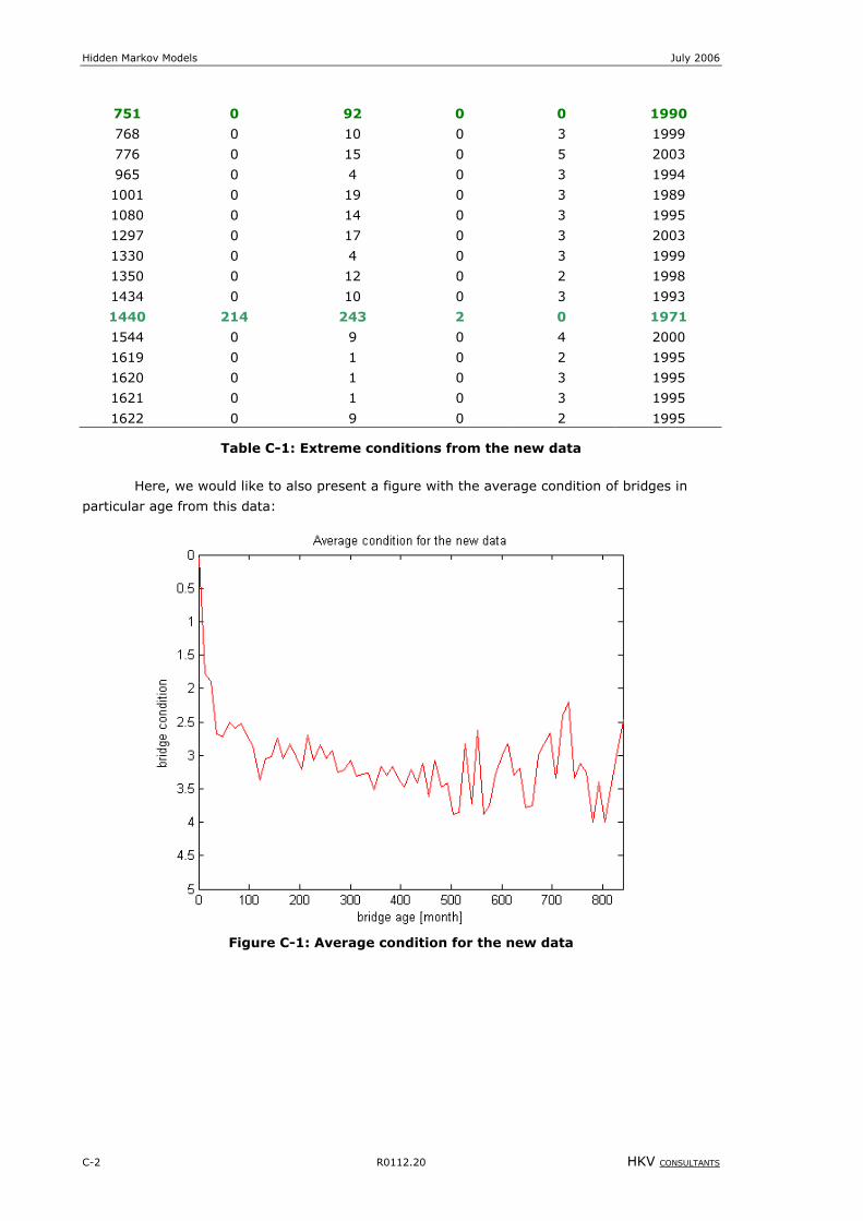
Hidden Markov Models July 2006
C-2 R0112.20 HKV CONSULTANTS
751 0 92 0 0 1990
768 0 10 0 3 1999
776 0 15 0 5 2003
965 0 4 0 3 1994
1001 0 19 0 3 1989
1080 0 14 0 3 1995
1297 0 17 0 3 2003
1330 0 4 0 3 1999
1350 0 12 0 2 1998
1434 0 10 0 3 1993
1440 214 243 2 0 1971
1544 0 9 0 4 2000
1619 0 1 0 2 1995
1620 0 1 0 3 1995
1621 0 1 0 3 1995
1622 0 9 0 2 1995
Table C-1: Extreme conditions from the new data
Here, we would like to also present a figure with the average condition of bridges in
particular age from this data:
Figure C-1: Average condition for the new data
July 2006 Hidden Markov Models
HKV CONSULTANTS R0112.20 D-1
Appendix D: Proof of the recursive formula (6-8), p.51
The proof is mainly the same as in the internship report (Appendix, [14]). The difference lies in
the fact that we have now the sequence of observations not equal j, and the additional not
complete sum over all states not equal to j needs to be involved into the formula.
We shall show that the conditional probability of the form:
(6-7) ),,...,Pr(),( 011 iXjOjOkXjk sss =≠≠== −φ
can be determined via the recursive formula:
(6-8)
∑∑
∑∑
≠∀−
=−−
−≠∀
−=
−−
⋅==
⋅==⋅===
jls
vss
sjl
ssu
ss
s
jvvXlO
juuXkXuXlOjk
),()Pr(
),()Pr()Pr(),(
1
5
011
11
5
011
φ
φφ
Proof:
Using the law of total probability, the previous specified assumptions and the rule of the
conditional probability, i.e.:
)Pr(),Pr()Pr(
BBABA =
we have:
==≠≠
=≠≠===≠≠==
−
−− ),,...,Pr(
),,...,,Pr(),,...,Pr(),(
011
011011 iXjOjO
iXjOjOkXiXjOjOkXjk
s
sssssφ
==≠≠
=≠≠===
−
=−−∑
),,...,Pr(
),,...,,,Pr(
011
5
00111
iXjOjO
iXjOjOuXkX
s
usss
==≠≠
=≠==⋅=≠==≠=
−
=−−−−−∑
),,...,Pr(
),..,,,Pr(),...,,,Pr(
011
5
00210211
iXjOjO
iXjOuXkXiXjOuXkXjO
s
usssssss
==≠≠
=≠≠=⋅==⋅=≠=
−
=−−−−−∑
),,...,Pr(
),,...,Pr()Pr()Pr(
011
5
00121111
iXjOjO
iXjOjOuXuXkXuXjO
s
ussssss
==≠≠
=≠=≠====≠=
−
−=
−−−−−∑),,...,Pr(
),.,Pr(),.,Pr()Pr()Pr(
011
02
5
0021111
iXjOjO
iXjOiXjOuXuXkXuXjO
s
su
ssssss
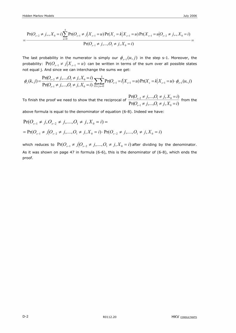
Hidden Markov Models July 2006
R0112.20 HKV CONSULTANTS D-2
==≠≠
=≠====≠=≠=
−
=−−−−−− ∑
),,...,Pr(
),.,Pr()Pr()Pr(),.,Pr(
011
5
002111102
iXjOjO
iXjOuXuXkXuXjOiXjO
s
usssssss
The last probability in the numerator is simply our ),(1 jus−φ in the step s-1. Moreover, the
probability: )Pr( 11 uXjO ss =≠ −− can be written in terms of the sum over all possible states
not equal j. And since we can interchange the sums we get:
∑∑≠∀ =
−−−−−
− ⋅=====≠≠=≠≠
=jl u
ssssss
ss juuXkXuXlO
iXjOjOiXjOjO
jk5
01111
011
012 ),()Pr()Pr(),,...,Pr(),,...,Pr(
),( φφ
To finish the proof we need to show that the reciprocal of ),,...,Pr(),,...,Pr(
011
012
iXjOjOiXjOjO
s
s
=≠≠=≠≠
−
− from the
above formula is equal to the denominator of equation (6-8). Indeed we have:
==≠≠≠ −− ),,....,,Pr( 0121 iXjOjOjO ss
),,....,Pr(),,....,Pr( 0120121 iXjOjOiXjOjOjO sss =≠≠⋅=≠≠≠= −−−
which reduces to ),,....,Pr( 0121 iXjOjOjO ss =≠≠≠ −− after dividing by the denominator.
As it was shown on page 47 in formula (6-6), this is the denominator of (6-8), which ends the
proof.
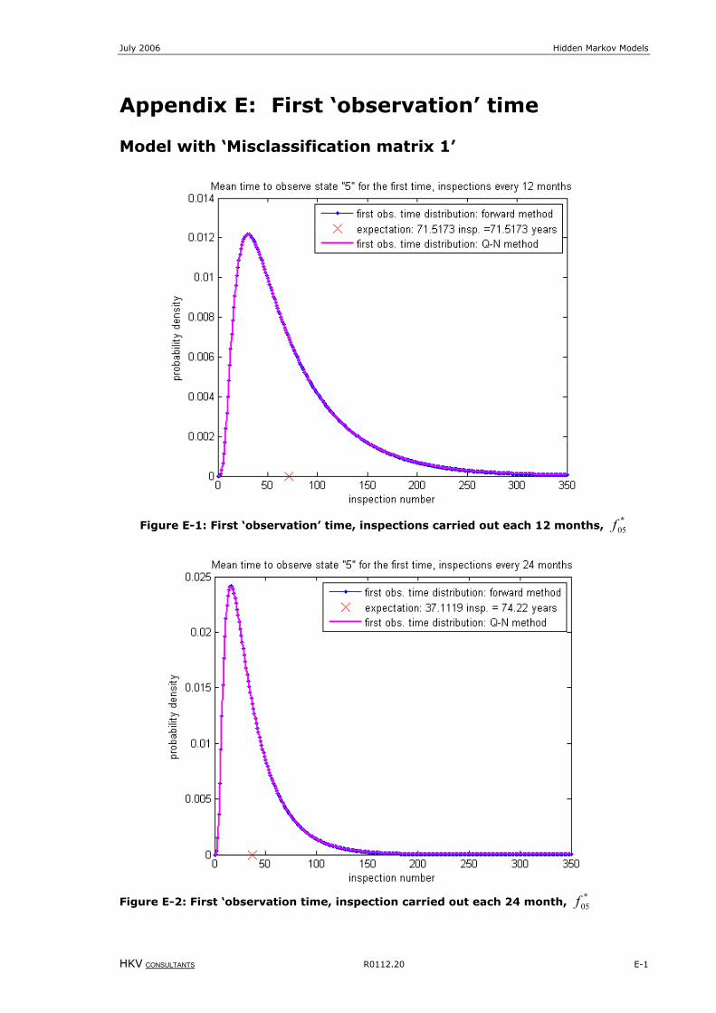
July 2006 Hidden Markov Models
HKV CONSULTANTS R0112.20 E-1
Appendix E: First ‘observation’ time
Model with ‘Misclassification matrix 1’
Figure E-1: First ‘observation’ time, inspections carried out each 12 months, *
05f
Figure E-2: First ‘observation time, inspection carried out each 24 month, *
05f
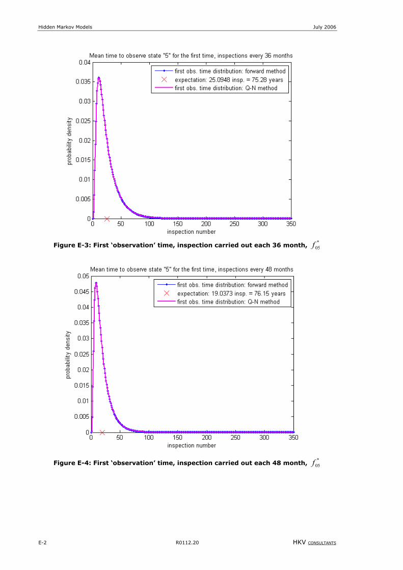
Hidden Markov Models July 2006
E-2 R0112.20 HKV CONSULTANTS
Figure E-3: First ‘observation’ time, inspection carried out each 36 month, *
05f
Figure E-4: First ‘observation’ time, inspection carried out each 48 month, *05f
July 2006 Hidden Markov Models
HKV CONSULTANTS R0112.20 E-3
Figure E-5: First ‘observation’ time, inspection carried out each 4800 month, *
05f
Model with ‘Misclassification matrix 2’
Figure E-6: First ‘observation’ time, inspection carried out each 12 month, *05f
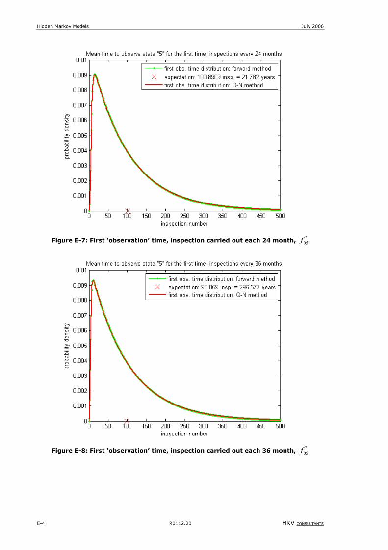
Hidden Markov Models July 2006
E-4 R0112.20 HKV CONSULTANTS
Figure E-7: First ‘observation’ time, inspection carried out each 24 month, *05f
Figure E-8: First ‘observation’ time, inspection carried out each 36 month, *05f
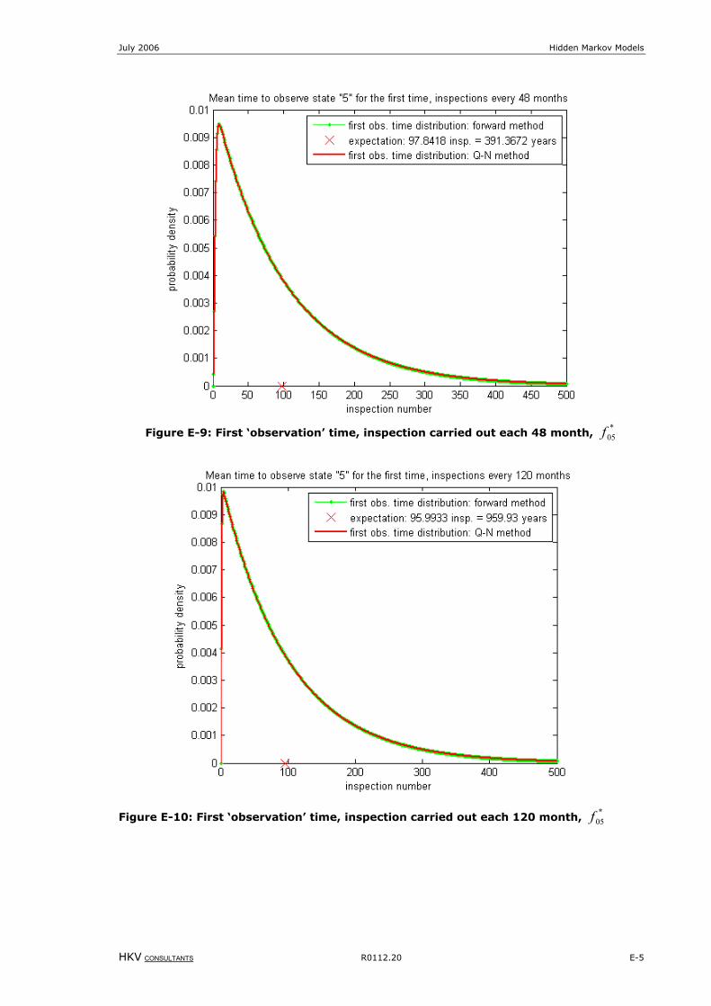
July 2006 Hidden Markov Models
HKV CONSULTANTS R0112.20 E-5
Figure E-9: First ‘observation’ time, inspection carried out each 48 month, *
05f
Figure E-10: First ‘observation’ time, inspection carried out each 120 month, *05f