MODELLING THE INFLUENCE OF BUILDINGS ON FLOOD FLOW

G. P. Smith1, C. D Wasko

1, B. M Miller

1

1 Water Research Laboratory, University of New South Wales, Sydney, NSW

Introduction Flood events in Newcastle in June 2007 and more recently in Queensland and Victoria in 2011 have highlighted the importance of having robust planning guidelines and building stability criteria for floodplains. These floods have also highlighted a requirement for accurate representation of flood hazard behaviour to support land use planning and flood evacuation planning documentation. Currently, the application of two-dimensional (2D) hydrodynamic (numerical) models has become a de-facto standard for baseline flood information for planning and management of Australian floodplains. However, the development, application and calibration of numerical models within this overall study scope have been open to considerable interpretation. Australian Rainfall and Runoff Revision Project 15: Two dimensional Simulation in Urban Areas has identified that one such aspect of 2D numerical model application for urban floodplains has been the method by which buildings and similar obstacles to flow are represented. Numerous methods have been devised to represent the influence of buildings on flood flow behaviour, including (Syme, 2008):

• Increased model roughness for building footprints;

• Blocking out model elements for building footprints;

• Modelling building exterior walls partially or in full;

• Using an energy loss coefficient over the building footprints; and

• Modelling buildings as ‘porous’ elements. The University of New South Wales Water Research Laboratory (WRL) recently completed a research program specifically investigating the role and influence of buildings on flooding in urban areas. The stated project objectives for the research were:

1. To develop a base dataset of reliable flood behaviour information (flow levels and depth,

flow distributions and flow velocities) for an urban floodplain; and

2. To test various methods for representing buildings in 2D numerical models with the aim of

determining a preferred method(s).

Literature Review A literature review of international journals and texts was completed to establish whether there was a readily available data set of flood behaviour for an urban area suitable to meet the second stated objective of the research. Based on the results of the literature review, the most rigorous method of verifying a numerical 2D urban flood model would be through replication of spatially correct flow distributions and velocities with a pre-requisite match of flood surface levels and inundation extent. The review determined that while there are numerous flood data sets, which have been collated from either measurement of historical floods or by measurement of physical scale models none of these datasets met the full set of specifications required for this study which were:

• High accuracy, high resolution topography;

• Water level data;

• Flow velocity data;

• Flow distribution data;

• Building footprint information;

• Building construction information;

• Anecdotal discussion of flood affectation of the buildings.

Hence the adopted approach for this study was to supplement available recorded data for a known historical flood with additional data measured in a scale physical model. The historical data set chosen was that of the June 2007 Flood in Merewether near Newcastle’s CBD. The data set was expanded by means of a scale physical model, suitably validated against available flood peak water levels in a flooded urban area.

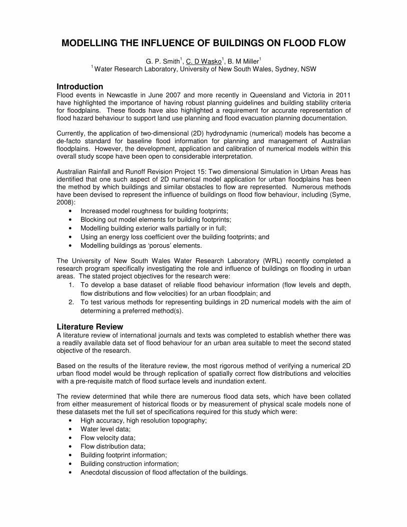
Test Case Site – Merewether NSW Newcastle has a long history of flooding both due to flash flooding and most recently, the city famously flooded in June 2007 in what has become known as the “Pasha Bulker” storm. The test site chosen for the physical model experiment was the overland flow path in the vicinity of Morgan Street, Merewether. The site is located just below the catchment divide at Merewether Heights (see Figure 1).

Figure 1: Test Site: Catchment Locality Plan

The Merewether site is attractive and suitable as a test site for this research. The severity of the flooding hazard during the June 2007 storm, the influence of buildings as obstructions to flow, the dendritic and somewhat constrained nature of the overflow path and availability of key data sets provides a location and data set which fits a wide range of criteria for a successful physical and numerical modelling exercise to meet the stated project objectives.

Available Data The Merewether site had a range of data suitable to meet the project requirements with the available data having a comparable coverage and accuracy limits representative of data standards typically available for a flood study in NSW.

Topography Newcastle City Council provided a Digital Elevation Model (DEM) that had been developed using photogrammetry with a stated vertical accuracy of ±0.2 m.

Indicative Study Catchment

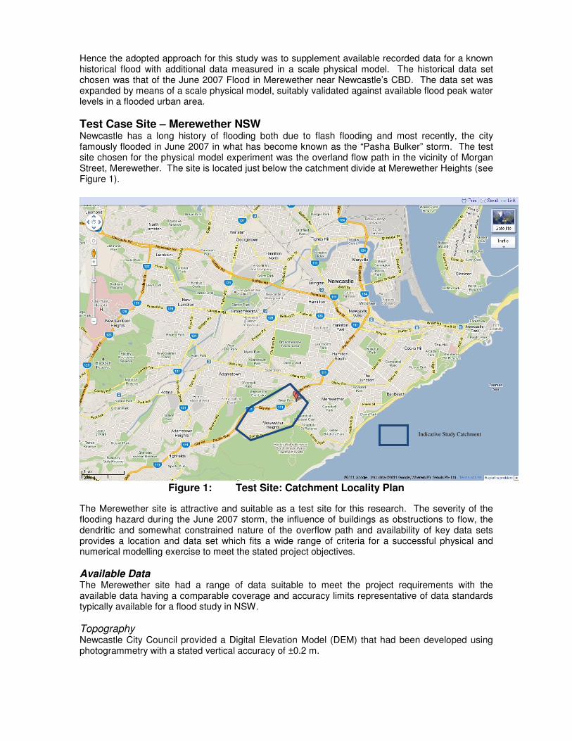
Rainfall The report by Haines et al. (2008) describing the “Pasha Bulker” storm of June 2007 has collated and analysed rainfall data recorded for the event (Figure 2). The measured Merewether 6-hour rainfall depth was approximately 240 mm compared to the 1:100 AEP 6-hour rainfall depth of 150 mm.

*Reproduced from Haines et al. (2008)

Figure 2: Comparison of 6-Hour Rainfall Depths to 1:100 AEP ARR (1987) Storm

Flood Marks Newcastle City Council and its consultants were diligent in collecting more than 1500 individual flood level marks immediately following the flood event in June 2007. Flood marks with surveyed peak water levels within the project site suitable for model calibration are presented in Table 1.

Table 1: Recorded Flood Marks, June 2007

Flood ID Level

(m AHD) Address Description

MWR_0031 19.985 10 Little Edward St, Merewether 1.23m up from concrete slab 5.3m from

back fence on wire fence

MWR_0032 18.382 75 Selwyn St, Merewether 180mm up from concrete veranda

adjacent to front door

MWR_0033 18.658 80A Wilton St, Merewether 300mm up from back pavers next to back

gauze door

MWR_0042 23.364 183 Morgan St, Merewether at ground on pebble 7.16 m from b/path

MWR_0043 23.14 174 Morgan St, Merewether at ground level, top of drive at base of

garage door

MWR_0044 23.014 170 Morgan St, Merewether up 320mm from concrete350mm up from

concrete step

Catchment Runoff Estimates The total sub-catchment area contributing flow to the project floodplain is 84 Ha. Being high in the catchment, the contributing catchment slopes are steep. The catchment is more or less bowl shaped, with the highest point in the south-west at 100 m AHD falling to the project area floodplain at 23 m AHD. The catchment is zoned residential and is fully developed.

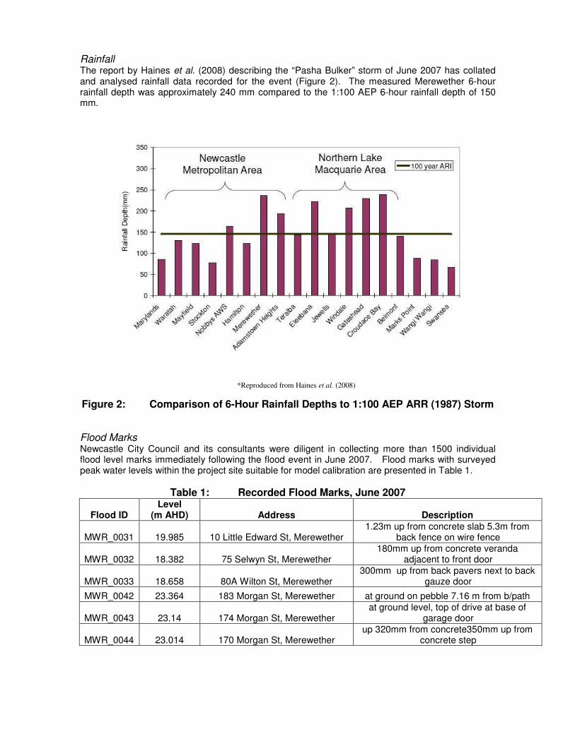
A WBMN model (Boyd et al. 2007) was developed as part of the Throsby, Cottage and CBD Flood Study by Syme and Ryan (2008) and made available for the project by Newcastle Council. The model had been validated as part of the flood study to previous historical floods. The WBNM model configuration file representative of existing catchment conditions from the flood study was adopted for this project. The model configuration was configured with June 2007 rainfall from the Merewether Street pluviometer gauge. Accumulated rainfall runoff estimated by the model at WBNM model provided the flow hydrograph presented as Figure 3. The peak flow rate in the hydrograph is 19.7 m

3/s. This compares to the 1:100 AEP 2 hour storm flow rate of 17.9 m

3/s and

the 1:200 AEP storm flow rate of 20.2 m3/s. This flow rate correlates well to analytical estimates of

flow based on the recorded flood slope and estimated surface roughness of the site.

Figure 3: WBNM Generated Runoff Hydrograph, June 2007

Physical Model The model domain adopted in both the physical and numerical models was selected following careful consideration of a range of constraints and parameters. A suitable model scale for the physical model able to adequately reproduce the flow behaviour of the prototype floodplain was primary amongst the wide range of constraints and parameters considered. The physical model scaling was determined using Froude similitude with assessment of Reynolds numbers used to ensure that flows in the physical model would be in the turbulent range.

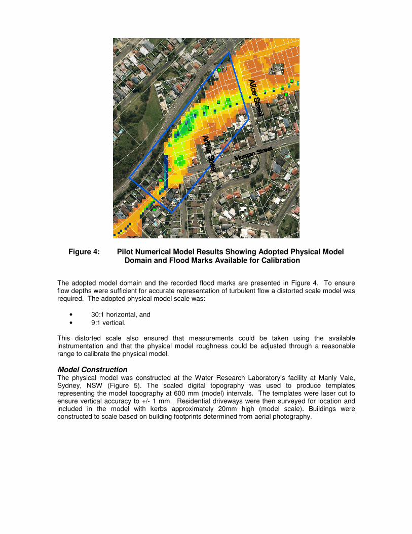
Figure 4: Pilot Numerical Model Results Showing Adopted Physical Model Domain and Flood Marks Available for Calibration

The adopted model domain and the recorded flood marks are presented in Figure 4. To ensure flow depths were sufficient for accurate representation of turbulent flow a distorted scale model was required. The adopted physical model scale was:

• 30:1 horizontal, and

• 9:1 vertical. This distorted scale also ensured that measurements could be taken using the available instrumentation and that the physical model roughness could be adjusted through a reasonable range to calibrate the physical model.

Model Construction The physical model was constructed at the Water Research Laboratory’s facility at Manly Vale, Sydney, NSW (Figure 5). The scaled digital topography was used to produce templates representing the model topography at 600 mm (model) intervals. The templates were laser cut to ensure vertical accuracy to +/- 1 mm. Residential driveways were then surveyed for location and included in the model with kerbs approximately 20mm high (model scale). Buildings were constructed to scale based on building footprints determined from aerial photography.

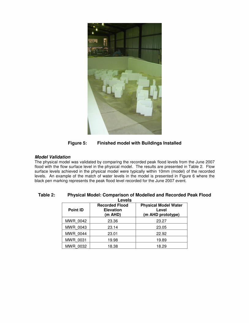
Figure 5: Finished model with Buildings Installed

Model Validation The physical model was validated by comparing the recorded peak flood levels from the June 2007 flood with the flow surface level in the physical model. The results are presented in Table 2. Flow surface levels achieved in the physical model were typically within 10mm (model) of the recorded levels. An example of the match of water levels in the model is presented in Figure 6 where the black pen marking represents the peak flood level recorded for the June 2007 event.

Table 2: Physical Model: Comparison of Modelled and Recorded Peak Flood Levels

Point ID Recorded Flood

Elevation (m AHD)

Physical Model Water Level

(m AHD prototype)

MWR_0042 23.36 23.27

MWR_0043 23.14 23.05

MWR_0044 23.01 22.92

MWR_0031 19.98 19.89

MWR_0032 18.38 18.29

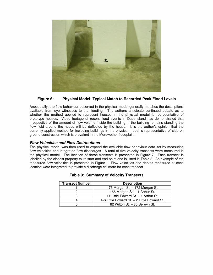
Figure 6: Physical Model: Typical Match to Recorded Peak Flood Levels

Anecdotally, the flow behaviour observed in the physical model generally matches the descriptions available from eye witnesses to the flooding. The authors anticipate continued debate as to whether the method applied to represent houses in the physical model is representative of prototype houses. Video footage of recent flood events in Queensland has demonstrated that irrespective of the amount of flow volume inside the building, if the building remains standing the flow field around the house will be deflected by the house. It is the author’s opinion that the currently applied method for including buildings in the physical model is representative of slab on ground construction which is prevalent in the Merewether floodplain.

Flow Velocities and Flow Distributions The physical model was then used to expand the available flow behaviour data set by measuring flow velocities and integrated flow discharges. A total of five velocity transects were measured in the physical model. The location of these transects is presented in Figure 7. Each transect is labelled by the closest property to its start and end point and is listed in Table 3. An example of the measured flow velocities is presented in Figure 8. Flow velocities and depths measured at each location were integrated to provide a discharge estimate for each transect.

Table 3: Summary of Velocity Transects

Transect Number Description

1 175 Morgan St. – 172 Morgan St.

2 166 Morgan St. – 1 Arthur St.

3 11 Little Edward St. – 1 Arthur St.

4 4-6 Little Edward St. – 2 Little Edward St.

5 82 Wilton St. – 80 Selwyn St.

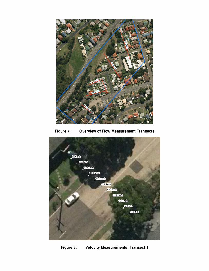
Figure 7: Overview of Flow Measurement Transects

Figure 8: Velocity Measurements: Transect 1

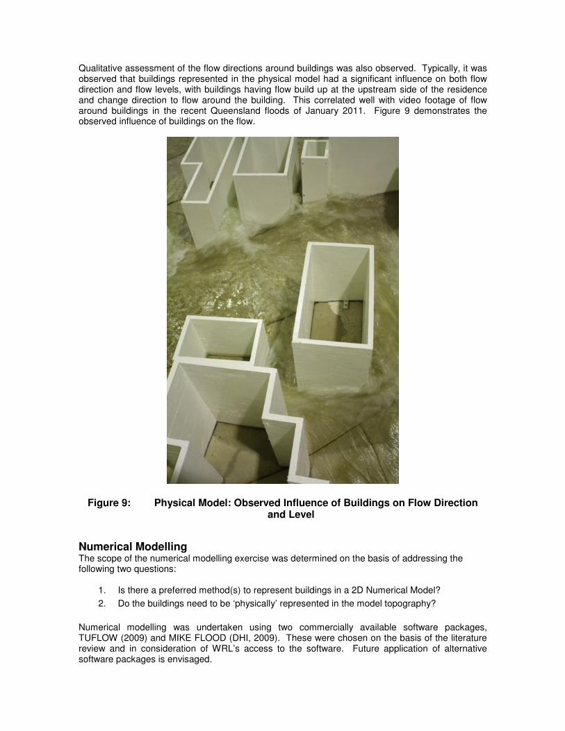
Qualitative assessment of the flow directions around buildings was also observed. Typically, it was observed that buildings represented in the physical model had a significant influence on both flow direction and flow levels, with buildings having flow build up at the upstream side of the residence and change direction to flow around the building. This correlated well with video footage of flow around buildings in the recent Queensland floods of January 2011. Figure 9 demonstrates the observed influence of buildings on the flow.

Figure 9: Physical Model: Observed Influence of Buildings on Flow Direction and Level

Numerical Modelling The scope of the numerical modelling exercise was determined on the basis of addressing the following two questions:

1. Is there a preferred method(s) to represent buildings in a 2D Numerical Model?

2. Do the buildings need to be ‘physically’ represented in the model topography?

Numerical modelling was undertaken using two commercially available software packages, TUFLOW (2009) and MIKE FLOOD (DHI, 2009). These were chosen on the basis of the literature review and in consideration of WRL’s access to the software. Future application of alternative software packages is envisaged.

Model Development The TUFLOW and MIKE FLOOD models were developed using identical data sets. The topography adopted for the numerical models was identical to that used as the basis of the physical model. The models were run using the flow hydrograph presented in Figure 3 with a constant downstream water level of 17.8 m AHD. The Manning’s ‘n’ roughness values were applied as listed in Table 4.

Table 4: Numerical Models: Adopted Manning’s ‘n’ Roughness Values Surface Manning’s ‘n’

Roads 0.020

Other areas 0.040

These roughness values were adopted following a calibration process, which involved adjusting model roughness parameters until a reasonable fit with recorded peak flood levels was achieved. The calibration adopted a model topography on a 1 m grid resolution with building footprints excluded from the model calculation. A comparison of the modelled and recorded peak water levels is provided in Table 5. The 1 m grid was adopted as a base case as it represented the prototype grid spacing that enabled at least two computational grid points in between all buildings in the model grid. The results show a reasonable match of modelled and recorded values has been achieved. Remarkably, the MIKE FLOOD and TUFLOW model results are within centimetres of each other. The behaviour of the two numerical models was found to be very similar in all simulations.

Table 5: Numerical Model: Comparison of Modelled and Recorded Peak Water Levels

Point ID

Recorded Flood

Elevation

MIKE FLOOD Peak Water

Level (m AHD)

Difference (m)

TUFLOW Peak Water

Level (m AHD)

Difference (m)

MWR_0042 23.36 23.57 0.21 23.56 0.20

MWR_0043 23.14 23.10 -0.04 23.11 -0.03

MWR_0044 23.01 22.79 -0.22 22.77 -0.24

MWR_0031 19.98 20.09 0.11 20.08 0.10

MWR_0032 18.38 18.34 -0.04 18.36 -0.02

MWR_0033 18.65 18.67 0.02 18.59 -0.06

Assessment Grid Resolution The influence of grid resolution on model results was tested by simulating models at four additional grid resolutions, using a 1 m grid as a base case, with buildings excluded from the model results. The additional grid resolutions tested were:

• 0.5 m;

• 2 m;

• 5 m; and

• 10 m.

In all simulations, the model roughness and other parameters were held constant. Results from each of the various model grid resolutions are presented below in Table 6.

Table 6: Numerical Model: Summary of the Influence of Grid Resolution on Peak Levels

Point ID

Recorded Flood

Elevation

1 m grid

(m AHD)

0.5 m grid

(m AHD)

2 m grid

(m AHD)

5 m grid

(m AHD)

10 m grid

(m AHD)

(m AHD)

MWR_0042 23.36 23.57 23.43 23.58 23.36 23.61

MWR_0043 23.14 23.10 22.91 23.11 23.14 23.13

MWR_0044 23.01 22.79 22.69 22.77 23.01 22.85

MWR_0031 19.98 20.09 19.85 20.09 19.98 20.30

MWR_0032 18.38 18.34 18.12 18.20 18.38 18.67

MWR_0033 18.65 18.67 18.47 18.67 18.65 19.46

The model results show that similar peak water levels are maintained for the 1 m and 2 m grids. Some ‘drift’ in peak water levels is noted outside the range of typically acceptable model calibration for the 5 m grid model with levels in the 10 m drifting by generally unacceptable increments. The 0.5 m model grid resolutions have also changed by a significant amount at some locations to the point where further consideration of model calibration parameters might need to be considered. Flow directions and velocities are reproduced consistently between the 0.5 m and 1 m grids. Flows at the 0.5 m, 1 m and 2 m grids generally match flow directions observed in the physical model with some minor changes are observable in the 2 m grid. Flow directions and flow path representation is noticeably different at the 5 m grid size and at the10 m grid resolution with numerous flow paths either not represented or with the flow direction and magnitude has markedly changed from the finer grid sizes. This is demonstrated in Figure 10 and Figure 11 which present the peak flood depths and velocities for the 1 m grid and 10 m grid respectively.

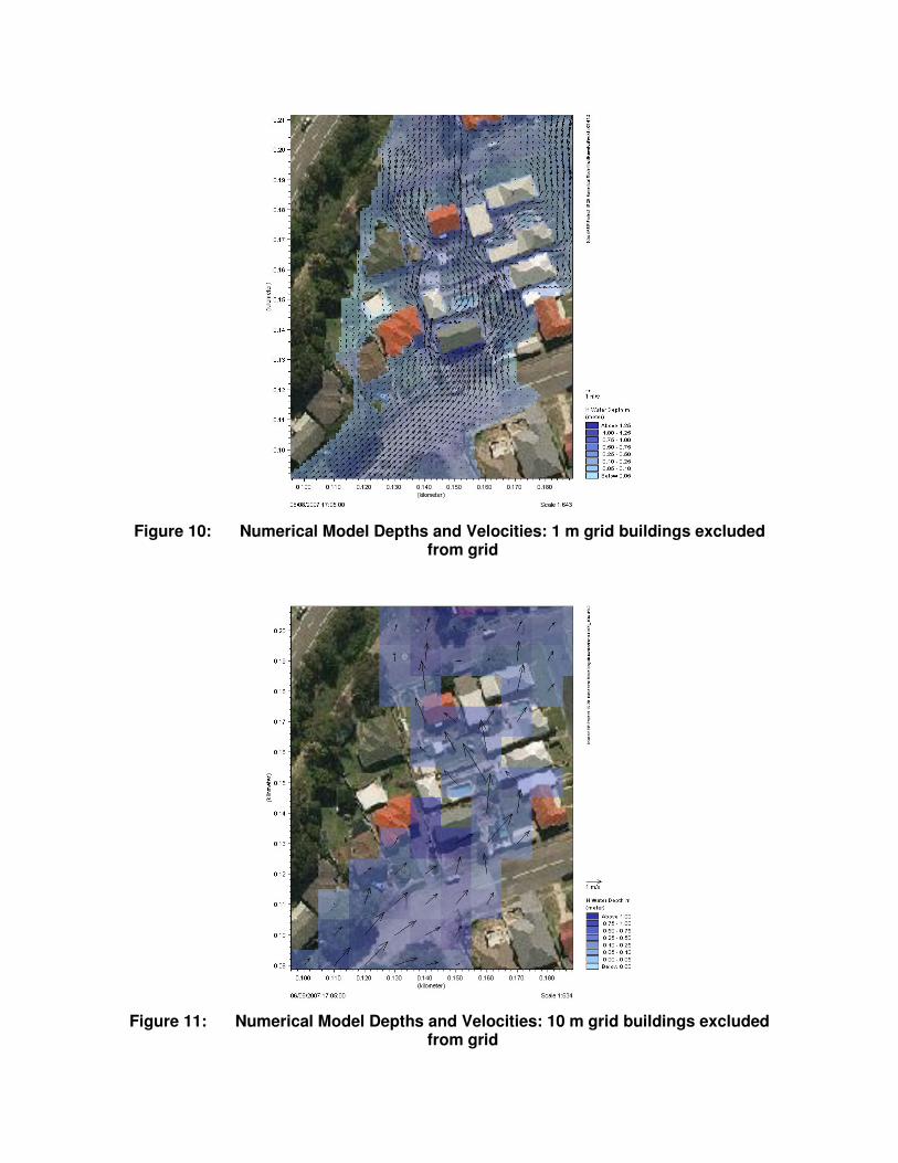
Figure 10: Numerical Model Depths and Velocities: 1 m grid buildings excluded

from grid

Figure 11: Numerical Model Depths and Velocities: 10 m grid buildings excluded

from grid

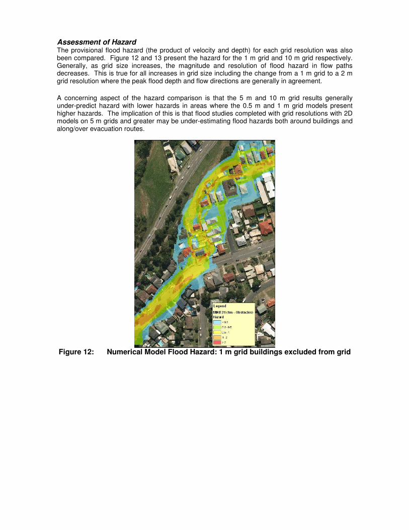
Assessment of Hazard The provisional flood hazard (the product of velocity and depth) for each grid resolution was also been compared. Figure 12 and 13 present the hazard for the 1 m grid and 10 m grid respectively. Generally, as grid size increases, the magnitude and resolution of flood hazard in flow paths decreases. This is true for all increases in grid size including the change from a 1 m grid to a 2 m grid resolution where the peak flood depth and flow directions are generally in agreement.

A concerning aspect of the hazard comparison is that the 5 m and 10 m grid results generally under-predict hazard with lower hazards in areas where the 0.5 m and 1 m grid models present higher hazards. The implication of this is that flood studies completed with grid resolutions with 2D models on 5 m grids and greater may be under-estimating flood hazards both around buildings and along/over evacuation routes.

Figure 12: Numerical Model Flood Hazard: 1 m grid buildings excluded from grid

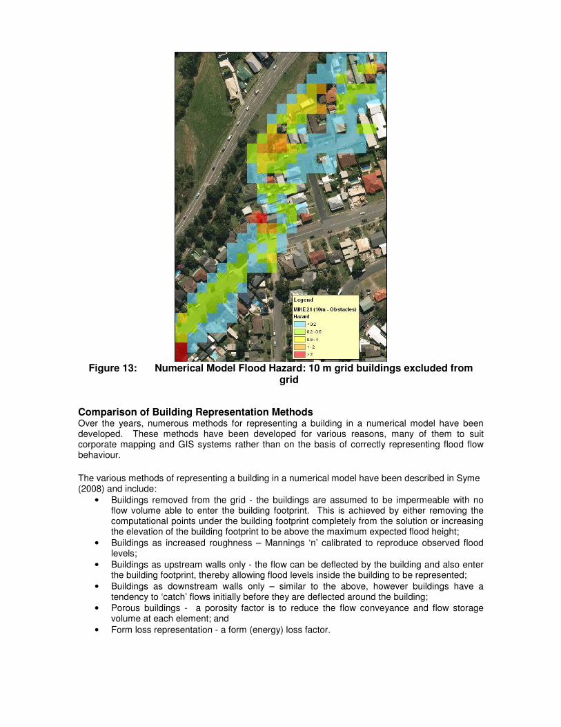
Figure 13: Numerical Model Flood Hazard: 10 m grid buildings excluded from

grid

Comparison of Building Representation Methods Over the years, numerous methods for representing a building in a numerical model have been developed. These methods have been developed for various reasons, many of them to suit corporate mapping and GIS systems rather than on the basis of correctly representing flood flow behaviour.

The various methods of representing a building in a numerical model have been described in Syme (2008) and include:

• Buildings removed from the grid - the buildings are assumed to be impermeable with no flow volume able to enter the building footprint. This is achieved by either removing the computational points under the building footprint completely from the solution or increasing the elevation of the building footprint to be above the maximum expected flood height;

• Buildings as increased roughness – Mannings ‘n’ calibrated to reproduce observed flood levels;

• Buildings as upstream walls only - the flow can be deflected by the building and also enter the building footprint, thereby allowing flood levels inside the building to be represented;

• Buildings as downstream walls only – similar to the above, however buildings have a tendency to ‘catch’ flows initially before they are deflected around the building;

• Porous buildings - a porosity factor is to reduce the flow conveyance and flow storage volume at each element; and

• Form loss representation - a form (energy) loss factor.

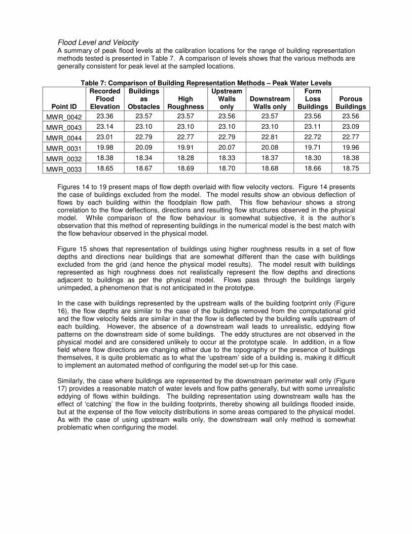
Flood Level and Velocity A summary of peak flood levels at the calibration locations for the range of building representation methods tested is presented in Table 7. A comparison of levels shows that the various methods are generally consistent for peak level at the sampled locations.

Table 7: Comparison of Building Representation Methods – Peak Water Levels

Point ID

Recorded Flood

Elevation

Buildings as

Obstacles High

Roughness

Upstream Walls only

Downstream Walls only

Form Loss

Buildings Porous

Buildings

MWR_0042 23.36 23.57 23.57 23.56 23.57 23.56 23.56

MWR_0043 23.14 23.10 23.10 23.10 23.10 23.11 23.09

MWR_0044 23.01 22.79 22.77 22.79 22.81 22.72 22.77

MWR_0031 19.98 20.09 19.91 20.07 20.08 19.71 19.96

MWR_0032 18.38 18.34 18.28 18.33 18.37 18.30 18.38

MWR_0033 18.65 18.67 18.69 18.70 18.68 18.66 18.75

Figures 14 to 19 present maps of flow depth overlaid with flow velocity vectors. Figure 14 presents the case of buildings excluded from the model. The model results show an obvious deflection of flows by each building within the floodplain flow path. This flow behaviour shows a strong correlation to the flow deflections, directions and resulting flow structures observed in the physical model. While comparison of the flow behaviour is somewhat subjective, it is the author’s observation that this method of representing buildings in the numerical model is the best match with the flow behaviour observed in the physical model. Figure 15 shows that representation of buildings using higher roughness results in a set of flow depths and directions near buildings that are somewhat different than the case with buildings excluded from the grid (and hence the physical model results). The model result with buildings represented as high roughness does not realistically represent the flow depths and directions adjacent to buildings as per the physical model. Flows pass through the buildings largely unimpeded, a phenomenon that is not anticipated in the prototype. In the case with buildings represented by the upstream walls of the building footprint only (Figure 16), the flow depths are similar to the case of the buildings removed from the computational grid and the flow velocity fields are similar in that the flow is deflected by the building walls upstream of each building. However, the absence of a downstream wall leads to unrealistic, eddying flow patterns on the downstream side of some buildings. The eddy structures are not observed in the physical model and are considered unlikely to occur at the prototype scale. In addition, in a flow field where flow directions are changing either due to the topography or the presence of buildings themselves, it is quite problematic as to what the ‘upstream’ side of a building is, making it difficult to implement an automated method of configuring the model set-up for this case. Similarly, the case where buildings are represented by the downstream perimeter wall only (Figure 17) provides a reasonable match of water levels and flow paths generally, but with some unrealistic eddying of flows within buildings. The building representation using downstream walls has the effect of ‘catching’ the flow in the building footprints, thereby showing all buildings flooded inside, but at the expense of the flow velocity distributions in some areas compared to the physical model. As with the case of using upstream walls only, the downstream wall only method is somewhat problematic when configuring the model.

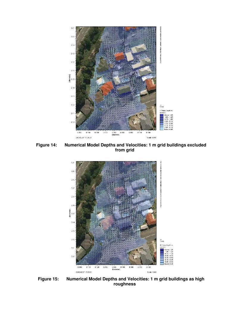
Figure 14: Numerical Model Depths and Velocities: 1 m grid buildings excluded

from grid

Figure 15: Numerical Model Depths and Velocities: 1 m grid buildings as high

roughness

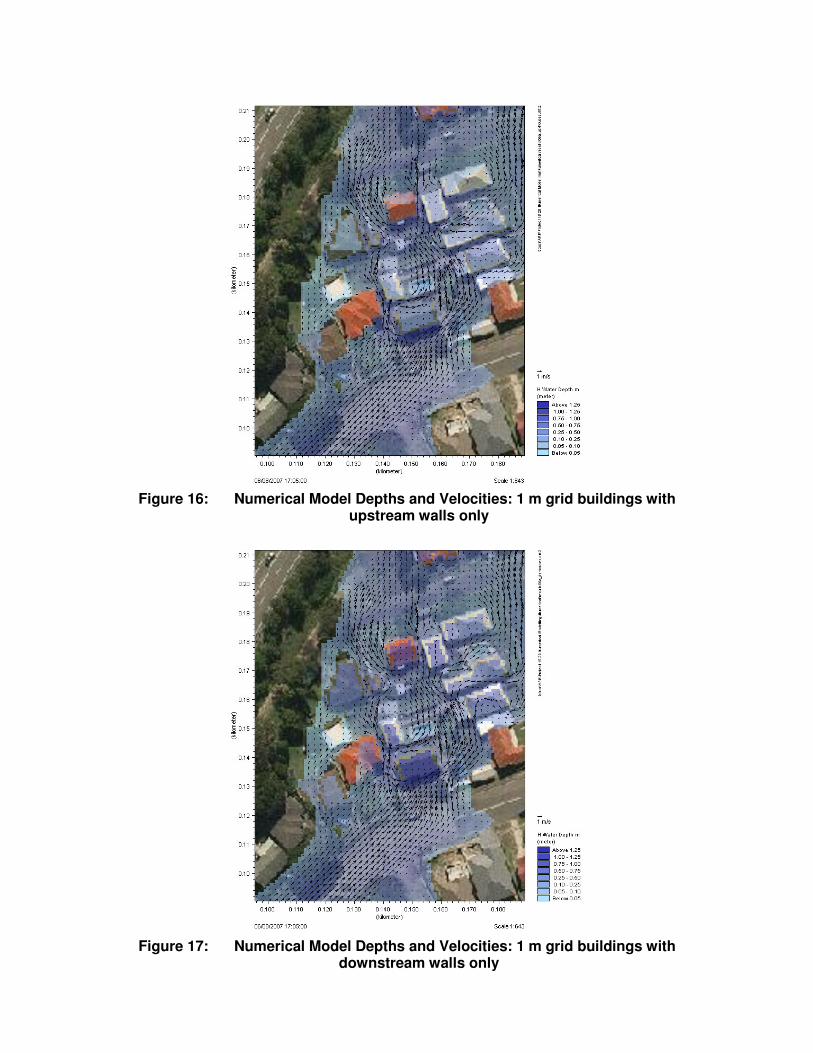
Figure 16: Numerical Model Depths and Velocities: 1 m grid buildings with

upstream walls only

Figure 17: Numerical Model Depths and Velocities: 1 m grid buildings with

downstream walls only

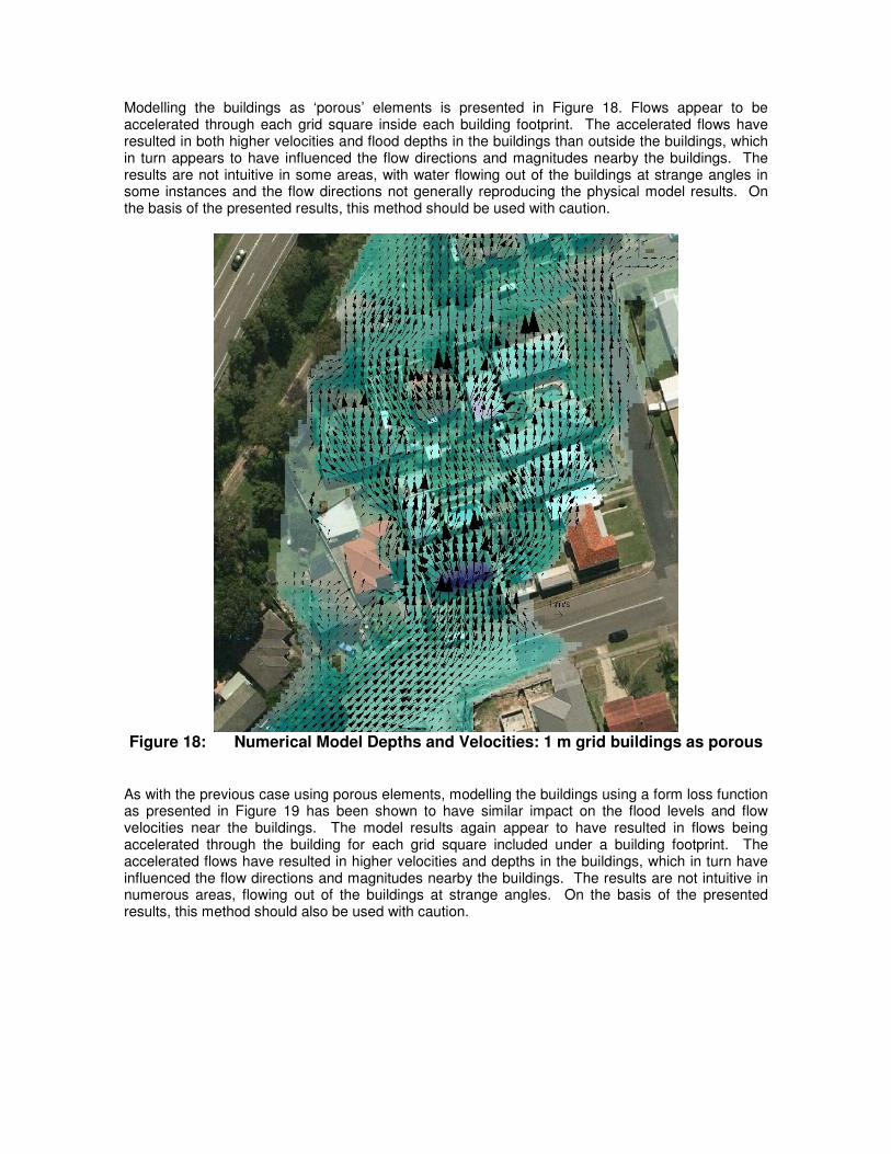
Modelling the buildings as ‘porous’ elements is presented in Figure 18. Flows appear to be accelerated through each grid square inside each building footprint. The accelerated flows have resulted in both higher velocities and flood depths in the buildings than outside the buildings, which in turn appears to have influenced the flow directions and magnitudes nearby the buildings. The results are not intuitive in some areas, with water flowing out of the buildings at strange angles in some instances and the flow directions not generally reproducing the physical model results. On the basis of the presented results, this method should be used with caution.

Figure 18: Numerical Model Depths and Velocities: 1 m grid buildings as porous

As with the previous case using porous elements, modelling the buildings using a form loss function as presented in Figure 19 has been shown to have similar impact on the flood levels and flow velocities near the buildings. The model results again appear to have resulted in flows being accelerated through the building for each grid square included under a building footprint. The accelerated flows have resulted in higher velocities and depths in the buildings, which in turn have influenced the flow directions and magnitudes nearby the buildings. The results are not intuitive in numerous areas, flowing out of the buildings at strange angles. On the basis of the presented results, this method should also be used with caution.

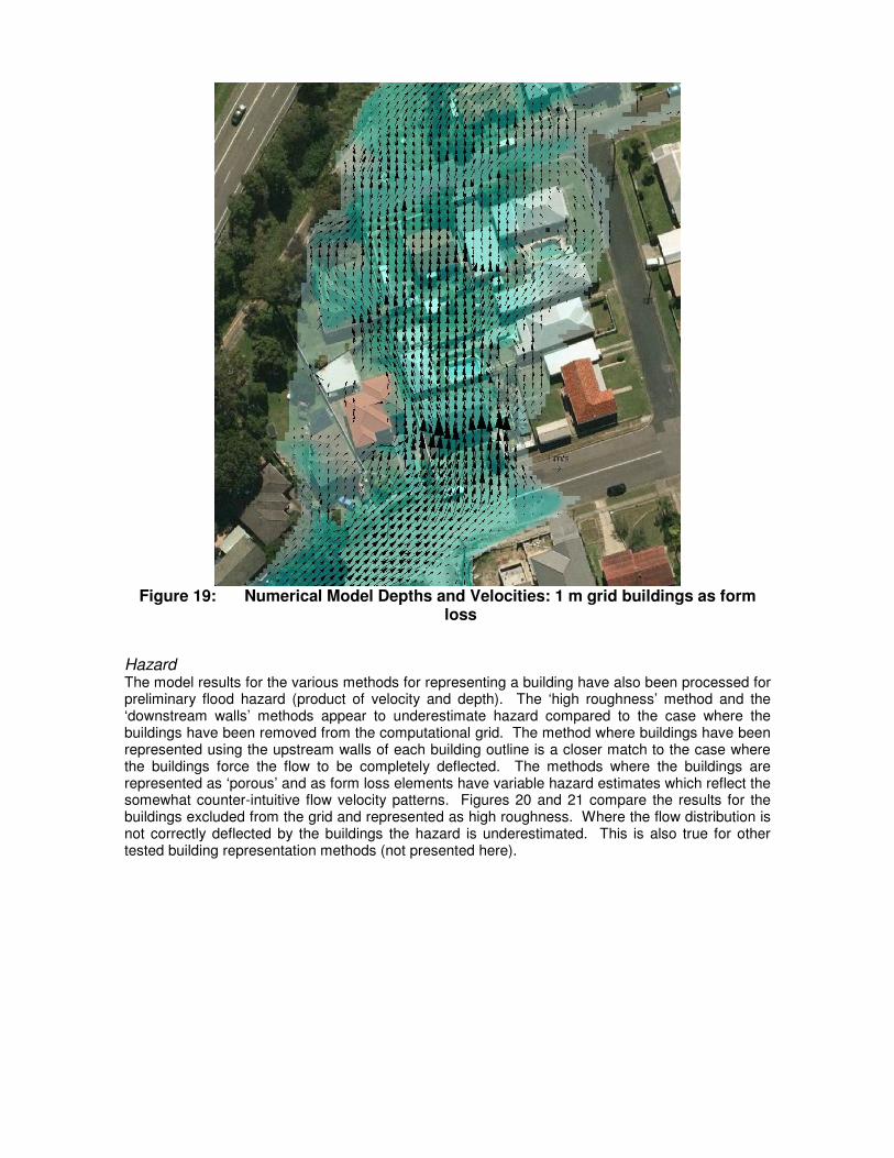
Figure 19: Numerical Model Depths and Velocities: 1 m grid buildings as form

loss

Hazard The model results for the various methods for representing a building have also been processed for preliminary flood hazard (product of velocity and depth). The ‘high roughness’ method and the ‘downstream walls’ methods appear to underestimate hazard compared to the case where the buildings have been removed from the computational grid. The method where buildings have been represented using the upstream walls of each building outline is a closer match to the case where the buildings force the flow to be completely deflected. The methods where the buildings are represented as ‘porous’ and as form loss elements have variable hazard estimates which reflect the somewhat counter-intuitive flow velocity patterns. Figures 20 and 21 compare the results for the buildings excluded from the grid and represented as high roughness. Where the flow distribution is not correctly deflected by the buildings the hazard is underestimated. This is also true for other tested building representation methods (not presented here).

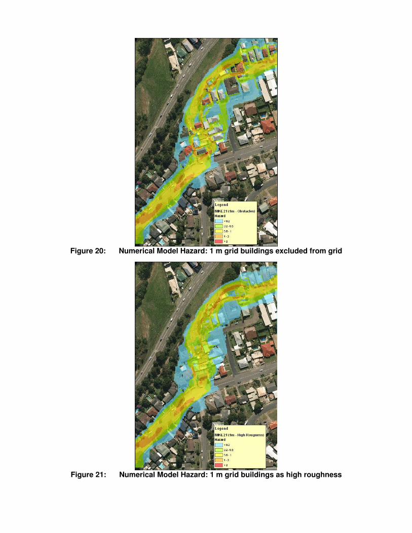
Figure 20: Numerical Model Hazard: 1 m grid buildings excluded from grid

Figure 21: Numerical Model Hazard: 1 m grid buildings as high roughness

Conclusions A physical model of the Merewether floodplain was constructed at the Water Research Laboratory (WRL), validated against historical flood information, and successfully used to expand the quantitative description of urban flood flow behaviour for the site in terms of flow velocities, flow directions and flow discharge distributions. A series of measurements of the physical model were then compared against similarly calibrated numerical models. Numerical models were developed using TUFLOW and MIKE FLOOD on the basis of their common use in the Australian market and the availability of these packages to WRL. Detailed analysis of the developed models including comparison of the models with observed data and data measured in the physical model has supported the conclusion that correctly discretised 2D numerical models are able to adequately represent observed flow behaviour on urban floodplains as long as a suitable method of representing buildings is applied. Analysis of numerical model results showed that the model spatial resolution is important for estimation of flood flow velocities, flow directions, flow discharge distributions and flood hazard definition. Hazard definition of flood flows is an important aspect of floodplain planning and flood emergency management and this investigation has concluded that numerical model resolutions should be carefully chosen so as to adequately represent flow hazard conditions. While model resolutions of up to 10 m were shown to be adequate for representing peak flood levels, model resolutions of 2m or less were required to represent the complex flow patterns in and around buildings on the floodplain. The results of the physical model assessment have shown that while buildings stand, they have a considerable influence on flood flow structures in urban environments, significantly deflecting flows irrespective of whether the building is flooded inside or remains water tight. Anecdotal evidence from videos of the recent Queensland Floods of January 2011 also shows buildings significantly deflecting flows when completely inundated and filled with flood water. It follows that this aspect of urban flow behaviour representation is important for faithful reproduction of flood behaviour in numerical models. The current investigation has shown that the method used to represent buildings in a numerical model is a key element required to match flow prototype flow patterns and the method must realistically deflect flows. In the project test case, some methods proposed in literature for representing the influence of buildings on flood flows were found to be deficient for that purpose. Numerical model trials showed that on the basis of the available data sets, the best performing method when representing buildings in a numerical model was to either remove the computational points under the building footprint completely from the solution or to increase the elevation of the building footprint to be above the maximum expected flood height. Other methods, while able to reproduce peak flood levels, were not able to satisfactorily reproduce flow distributions and flow directions around buildings on the floodplain. It follows that flood hazard would only be satisfactorily reproduced using these methods.

References Australian Rainfall & Runoff, A Guide to Flood Estimation (ARR, 1987), Institution of Engineers, Australia (1987) Vol1. Boyd, M., Rigby, E., and VanDrie, R. (2007) Watershed Bound Network Model (WBNM) Version 1.04, January 2007. DHI (2009), “MIKE FLOOD 1D-2D Modelling User Manual”, DHI Software.

Haines P., Rollason V., Kidd L. and Wainwright D. (2008) 8 June 2007, (the Pasher Bulker Storm), Flood Data Compendium”, Final Report prepared by BMTWBM for Newcastle City Council, May 2008 R.N0722.001.01. Syme, W. J. and Ryan P. (2008), “Throsby, Cottage and CBD Flood Study”, Report prepared for Newcastle City Council, August 2008, RB15058.002.01. Syme W. J. (2008) Flooding in Urban Areas – 2D Modelling Approaches for Buildings and Fences. Engineers Australia, 9

th National Conference on Hydraulic in Water Engineering. Darwin Convention

Centre, Australia 23-36 September 2008. TUFLOW (2009), “TUFLOW User Manual, GIS Based 2D/1D Hydrodynamic Modelling”, BMT WBM