Modelling the evolution of credit spreads using the Cox process within the HJM framework: A CDS option pricing model

European Journal of Operational Research 208 (2011) 95–108

Contents lists available at ScienceDirect

European Journal of Operational Research

journal homepage: www.elsevier .com/locate /e jor

Invited Review

Modelling the evolution of credit spreads using the Cox process within the HJMframework: A CDS option pricing model

Carl Chiarella a, Viviana Fanelli b,*, Silvana Musti b

a School of Finance and Economics, University of Technology, Sydney, P.O. Box 123, Broadway, NSW 2007, Australiab Dipartimento di Scienze Economiche, Matematiche e Statistiche, Università degli Studi di Foggia, Largo Papa Giovanni Paolo II, 1, 71100, Foggia, Italy

a r t i c l e i n f o

Article history:Received 20 October 2008Accepted 1 March 2010Available online 10 March 2010

Keywords:PricingHJM modelCox processMonte Carlo methodCDS option

0377-2217/$ - see front matter � 2010 Elsevier B.V. Adoi:10.1016/j.ejor.2010.03.006

* Corresponding author. Fax: +39 0881 775616.E-mail addresses: [email protected] (C. Chi

a b s t r a c t

In this paper a simulation approach for defaultable yield curves is developed within the Heath et al.(1992) framework. The default event is modelled using the Cox process where the stochastic intensityrepresents the credit spread. The forward credit spread volatility function is affected by the entire creditspread term structure. The paper provides the defaultable bond and credit default swap option price in aprobability setting equipped with a subfiltration structure. The Euler–Maruyama stochastic integralapproximation and the Monte Carlo method are applied to develop a numerical scheme for pricing.Finally, the antithetic variable technique is used to reduce the variance of credit default swap optionprices.

� 2010 Elsevier B.V. All rights reserved.

1. Introduction

Since the 1990s, the focus on credit risk has increased amongst academics and financial market practitioners. This is due to the concernsof regulatory agencies and investors regarding the high exposure of financial institutions to over-the-counter derivatives. It is also due tothe rapid development of markets for price-sensitive and credit-sensitive instruments that allow institutions and investors to trade thisrisk.

The new Basel accord (International Convergence of Capital Measurement and Capital Standard, Basel II, 26 January 2004) promotes thestandards for credit risk management, obligating financial institutions to fulfill a variety of regulatory capital requirements. By increasingthe reliability of the credit derivative market, the Basel II rules have contributed to its success.

In the credit risk literature two principal kinds of models are widely used: the structural models and the reduced form models.Structural models were proposed by Merton (1974), Black and Cox (1976), Shimko et al. (1993) and Longstaff and Schwartz (1995), to

cite the principal contributions. These models focus on the analysis of a firm’s structural variables: the default event derives from the evo-lution of the firm’s assets and it is completely specified in an endogenous way.

The main drawback of the structural approach is that since many of the firm’s assets are typically not traded, the firm’s value process isfundamentally unobservable, making implementation difficult. Furthermore, this approach assumes that only bonds with homogeneouslevels of seniority exist and that the risk-free rates are constant over the period of evaluation.

Zhou (1997) and Schönbucher (1996) are two important contributions that use jump diffusion processes for the evolution of the firm’svalue in the Merton model. These models are more realistic in generating the shape of a credit spread term structure compared to the clas-sical structural models that seem to underestimate credit spread values. Jump-diffusion models also have the advantage of allowing thedefault event to occur abruptly.

Reduced form models are characterized by a more flexible approach to credit risk. They mainly model the spread between the defaul-table interest rate and the risk-free rate. The default time is a stochastic variable modelled as a stopping time. The two earliest contribu-tions to this approach are those of Jarrow and Turnbull (1995) and Jarrow et al. (1997).

Jarrow and Turnbull (1995) consider a constant and deterministic Poisson intensity. In contrast, Jarrow et al. (1997) consider the issuer’srating as the fundamental variable driving the default process and the rating dynamics are modelled as a Markov chain, where default is theabsorbing state.

ll rights reserved.

arella), [email protected] (V. Fanelli), [email protected] (S. Musti).

http://dx.doi.org/10.1016/j.ejor.2010.03.006

mailto:[email protected]



http://www.sciencedirect.com/science/journal/03772217

http://www.elsevier.com/locate/ejor

96 C. Chiarella et al. / European Journal of Operational Research 208 (2011) 95–108

Lando (1998) uses a stochastic intensity, while the default process is described by a Cox process which allows a remarkable degree ofanalytical tractability. The Cox process is a generalization of the Poisson process when the intensity is random. If the Cox process is con-ditional on a particular realization of the intensity, it becomes an inhomogeneous Poisson process.

Das and Sundaram (2000) find a more flexible pricing methodology valid both for bonds and credit derivatives. A defaultable bond priceis equal to the expected value of future payoffs discounted by a defaultable interest rate. The term structure models existing in the liter-ature, such as Cox et al. (1985) and Heath et al. (1992) can then be used to model the defaultable term structure.

An important result demonstrated in Duffie and Lando (2001) is the way in which a structural model of the Black and Cox (1976) type isconsistent with the reduced form class of models when asymmetric information about structural characteristics is revealed.

Recently, academics and practitioners have utilized the risk-neutral pricing methodology to carry out credit spread term structure anal-ysis. Duffie and Singleton (1999) provide a discrete-time reduced form model in order to evaluate risky debt and credit derivatives in anarbitrage-free environment. They add a forward spread process to the forward risk-free rate process and use the Heath et al. (1992) ap-proach to obtain the arbitrage-free drift restriction and by using the ”Recovery of Market Value” condition (Duffie and Singleton, 1999),they provide a recursive formula that is easy to implement.

The HJM approach is used by Schönbucher (1998) in order to model the term structure of defaultable interest rates. The defaultablebond price is obtained under the following assumptions: (i) positive recovery rates, (ii) reorganization of the defaulted firms with the pos-sibility of multiple default, and (iii) uncertainty about the magnitude of the default. Furthermore, the firm’s default causes jumps in thedefaultable interest rate process. Using the HJM approach, Schönbucher (1998) provides a drift restriction for the defaultable term struc-ture. A similar result is obtained in Pugachevsky (1999), where the HJM drift restriction is obtained by applying the arbitrage-free conditionobtained in Maksyumiuk and Gtarek (1999) and without assuming any jumps to default.

Finally, Jeanblanc and Rutkowski (2002), Jamshidian (2004) and Brigo and Morini (2005) suggest a different approach to defaultablebond and credit derivative modelling: in a probability space equipped with a subfiltration structure the default is modelled as a Cox pro-cess. Furthermore, Chen et al. (2008) provide a model for valuing a credit default swap when the interest rate and the hazard rate are cor-related. They provide an explicit solution to the model by solving a bivariate Riccati equation. Their model is solved quickly so that all theparameters of the model are simultaneously estimated.

In this paper, we build on the cited recent literature and develop a model for credit spread term structure evolution and credit derivativepricing. The HJM model has been extensively analyzed in the literature from a theoretical point of view: our intent, instead, is to focus onthe applications of the model for pricing purposes. In particular, we model the forward credit spread curve within the HJM frameworkusing the theory of Cox processes where the stochastic intensity represents the credit spread. The HJM model is known to be one of themost general term structure models and for this reason we have chosen to extend its interest rate dynamics to the defaultable rate: theforward credit spread volatility function, the initial credit spread curve and specifications of the volatility structure are the sole inputs. Be-cause of the arbitrage-free condition, the drift can be expressed in terms of the volatility. We assume a stochastic volatility for both therisk-free interest rate and the credit spread, so that analytical results are not readily available and model implementation is generally pos-sible only via a numerical simulation approach. We develop and implement an efficient numerical scheme that allows bond and creditderivative pricing. The accuracy of the calculated values is improved by the application of a well known method of variance reduction,the antithetic variable technique.

In Section 2 we describe the model. In Section 3 we outline the foundations of credit default swap (CDS) pricing and derive CDS optionpricing formulae under the equivalent martingale measure. In Section 4 we outline the application of Monte Carlo simulation to the HJMmodel based on the Euler–Maruyama discretisation of the forward rate dynamics. A variance reduction technique is applied to improve theefficiency of the Monte Carlo method and to provide more accurate numerical results for pricing. Then, the efficiency of the computationaltechnique in terms of runtimes is investigated. The analysis concerning the runtime/accuracy trade-off indicates how the evaluation meth-od can be successfully utilized by credit risk practitioners who wish to price credit risk products with satisfactory levels of accuracy andreasonable runtimes. Section 5 concludes.

2. Model setting

The model is set in a filtered probability space ðX;F; ðFtÞtP0;PÞ, T is assumed to be the finite time horizon and F ¼FT is the r-algebraat time T . All statements and definitions are understood to be valid until the time horizon T. The probability space is assumed to be largeenough to support both an Rd-valued stochastic process X ¼ fXt : 0 6 t 6 Tg that is right-continuous with left limit, and a Poisson processNðtÞ with Nð0Þ ¼ 0, independent of X.

The background driving process X generates the subfiltration H ¼ ðHtÞtP0 ¼ ðrðXs : 0 6 s 6 tÞÞtP0 representing the flow of all back-ground information except default itself and H ¼HT is the sub-r-algebra at time T.

The Poisson process NðtÞ has a non negative and right-continuous stochastic intensity kðtÞ which is independent of NðtÞ and follows thediffusion process

dkðtÞ ¼ lkðtÞdt þ rkðtÞdWkðtÞ; ð1Þ

where lkðtÞ is the drift of the intensity process, rkðtÞ is the volatility of the intensity process and Wk is a standard Wiener process under theobjective probability measure P. The intensity process kðtÞ is assumed to be adapted to H, and the assumption of time dependent intensityimplies the existence of an inhomogeneous Poisson process.

In the subfiltration setting outlined above it is natural to consider an Ht-conditional Poisson process in such a way that a Cox process isassociated with the state variables process X and the intensity function kðtÞ. We define si; i 2 N, as the times of default generated by the Coxprocess NðtÞ ¼

P1i¼11fsi6tg with intensity kðtÞ. We only consider the time of the first default and it will be referred to with s :¼ s1. Then, the

defaultable time s is a stopping time, s : X! Rþ0 , defined as the first jump time of NðtÞ,

s ¼ infft 2 Rþ0 jNðtÞ > 0g:

C. Chiarella et al. / European Journal of Operational Research 208 (2011) 95–108 97

The right-continuous default indicator process 1fs6tg generates the subfiltration Fs ¼ ðFst ÞtP0 ¼ ðrð1fs6sg : 0 6 s 6 tÞÞtP0, that is assumed

to be one component of the full filtration F ¼ ðFtÞtP0. Since obviously Fst �Ft ;8t 2 Rþ0 , s is a stopping time with respect to F, but it is not

necessarily a stopping time with respect to H. It follows that F ¼ H _ Fs, that is Ft ¼Ht _ Fst 8t 2 Rþ0 .

For any t 2 Rþ0 , we define the default probability as Pðs 6 tjHtÞ and the survival probability as Pðs > tjHtÞ. These two quantities indi-cate, respectively, the probability of default occurring or not occurring up to time t. In the subfiltration setting, asset pricing is consistentwith the application of the iterated expectation law.

At any time t, the risk-free zero coupon bond price is denoted by Pðt; TÞ, where T represents the maturity time, T > t, and it is calculatedaccording to

Pðt; TÞ ¼ e�R T

tf ðt;sÞds

; ð2Þ

where f ðt; TÞ is the instantaneous risk-free forward rate at time t applicable at fixed maturity T. Conversely, if the derivative of Pðt; TÞ withrespect to maturity T exists, the instantaneous risk-free forward rate can be written in terms of the bond price as

f ðt; TÞ ¼ � @

@TlogPðt; TÞ: ð3Þ

We assume that the forward rate is driven by the diffusion process

df ðt; TÞ ¼ aðt; T; �Þdt þ rðt; T; �ÞdWðtÞ; ð4Þ

where aðt; T; �Þ is the instantaneous forward rate drift function, rðt; T; �Þ is the instantaneous forward rate volatility function and WðtÞ is astandard Wiener process with respect to the objective probability measure P. The third argument in the brackets ðt; T; �Þ indicates the pos-sible forward rate dependence on other path dependent quantities, such as the spot rate or the forward rate itself. The instantaneous risk-freeshort rate rðtÞ is defined as rðtÞ :¼ f ðt; tÞ.

We recall that the HJM no-arbitrage drift restriction is

aðt; T; �Þ ¼ rðt; T; �ÞZ T

trðt; s; �Þds� /ðtÞ

� �: ð5Þ

Similar statements hold for defaultable bonds. We indicate with Pd;Rðt; TÞ the generic price at any time t of a defaultable zero couponbond with maturity T and recovery rate R. If we set

Pdðt; TÞ :¼ Pd;0ðt; TÞ;
we have
Pdðt; TÞ ¼ 1fs>tge�R T

tfdðt;sÞds

; ð6Þ

where fdðt; TÞ is the instantaneous defaultable forward rate at time t applicable to fixed maturity T. If the derivative of Pdðt; TÞwith respect tomaturity T exists and assuming that the default occurs after t, the instantaneous defaultable forward rate can be written in terms of the bondprice as

fdðt; TÞ ¼ �@

@TlogPdðt; TÞ ð7Þ

and is assumed to be modelled by the stochastic process

dfdðt; TÞ ¼ adðt; T; �Þdt þ rdðt; T; �ÞdWdðtÞ; ð8Þ
where adðt; T; �Þ and rdðt; T; �Þ are, respectively, the drift function and the volatility function of the instantaneous defaultable forward rate.Furthermore WdðtÞ is a standard Wiener process with respect to the objective probability measure P. As in (4), the third argument in thebrackets ðt; T; �Þ indicates, again, the possible defaultable forward rate dependence on other path dependent quantities, such as the defaul-table spot rate or the defaultable forward rate itself.
Spot rate dynamics are derived from the forward rate dynamics, since rdðtÞ :¼ fdðt; tÞ. Recalling that the market is arbitrage-free if andonly if there exists a probability measure eP such that discounted asset price processes are martingales, the defaultable bond price is nowobtained as the risk-neutral expectation of the discounted bond value, namely

Pdðt; TÞ ¼ 1fs>tgEeP ½e�R T

trdðsÞdsjHt� ð9Þ

where e�R T

trdðsÞds is the defaultable stochastic discount factor and eP is the risk-neutral equivalent probability measure.

Following Lando (1998), the pricing formula at time t for a defaultable zero coupon bond with maturity T is given by

Pdðt; TÞ ¼ EeP ½e�R T

trðsÞds

1fs>TgjFt � ¼ EeP ½EeP ½e�R T

trðsÞds

1fs>TgjHT _Fst �jFt � ¼ EeP ½e�R T

trðsÞds

1fs>tgEeP ½1fs>TgjHT _Fst �jFt �

¼ 1fs>tgEeP ½e�R T

tðrðsÞþkðsÞÞdsjFt� ¼ 1fs>tgEeP ½e�R T

tðrðsÞþkðsÞÞdsjHt �: ð10Þ

The last equation follows from the law of iterated expectations. Comparing Eq. (9) with Eq. (10), we see that the default free and defaul-table instantaneous spot rate are related by

rdðtÞ ¼ rðtÞ þ kðtÞ; ð11Þ
where kðtÞ is the (stochastic) intensity rate. So the credit spread at the short end is kðtÞ. Eq. (11) suggests writing the credit spread acrossrates of all maturities as ksðt; TÞ so that
fdðt; TÞ ¼ f ðt; TÞ þ ksðt; TÞ: ð12Þ


We assume for ksðt; TÞ the dynamics

ksðt; TÞ ¼ ksð0; TÞ þZ t

0akðs; T; �Þdsþ

Z t

0rkðs; T; �ÞdWkðsÞ; ð13Þ

where akðt; T; �Þ is the drift, rkðt; T; �Þ is the volatility of the credit spread curves and WkðtÞ is a standard Wiener process under P. For (11) and(12) to be compatible at T ¼ t we must have

kðtÞ ¼ ksðt; tÞ: ð14Þ

From (13) it follows that the stochastic integral equation for kðtÞ may be written

kðtÞ ¼ ksðt; tÞ ¼ ksð0; tÞ þZ t

0akðs; t; �Þdsþ

Z t

0rkðs; t; �ÞdWkðsÞ; ð15Þ

from which (the subscript 2 denotes partial derivative with respect to the second argument)

dkðtÞ ¼ akðt; t; �Þ þZ t

0ak2 ðs; t; �Þdsþ

Z t

0rk2 ðs; t; �ÞdWkðsÞ

� �dt þ rkðt; t; �ÞdWkðtÞ: ð16Þ

Thus in order that (1) and (16) be compatible it must be the case that the lkðtÞ and rkðtÞ in Eq. (1) are given by

lkðtÞ ¼ akðt; t; �Þ þZ t

0ak2 ðs; t; �Þdsþ

Z t

0rk2 ðs; t; �ÞdWkðsÞ; rkðtÞ ¼ rkðt; t; �Þ:

For simplicity of expression we shall assume stochastic differential equations driven by one Brownian motion for both the risk-free for-ward rate and the credit spread. Consequently, the correlation between the Brownian motions dW and dWk becomes a scalar coefficientthat we write as

q ¼ corrðdW;dWkÞ: ð17Þ

We use the Heath et al. (1992) approach to model the term structure of defaultable interest rates. The main advantages of the HJM mod-el are that in the formulation of the spot rate process and bond price process the market price of interest rate risk drops out by being incor-porated into the Wiener process under the risk-neutral measure; the model is automatically calibrated to the initial yield curve and thedrift term in the forward rate differential equation is a function of the volatility term. As result of the latter characteristic, the HJM modelcan be considered as a class of models, each one identified by the choice of a volatility function. Consequently, we need to give a specificfunctional form to the volatility term in order to obtain a specific HJM model. The main complication of this approach is that some volatilityfunctions make the dynamics for rðtÞ and rdðtÞ path dependent, in other words non-Markovian, and since the bond price dynamics dependon these, they also become non-Markovian making the model difficult to handle, both analytically and numerically.

Using the HJM approach, we show in Appendix B that the no-arbitrage restriction on the drift of the credit spread process may be writ-ten as

akðt; TÞ ¼ q rðt; TÞZ T

trkðt; sÞdsþ rkðt; TÞ

Z T

trðt; sÞds

� �dv þ rkðt; TÞ

Z T

trkðt; sÞds� rkðt; TÞ/kðtÞ:

so that the stochastic dynamics for the defaultable forward rate, written in integral form, are

fdðt; TÞ ¼ f ð0; TÞ þ ksð0; TÞ þZ t

0rðv; TÞ

Z T

vrðv ; sÞdsþ rkðv; TÞ

Z T

vrkðv ; sÞds

� �dv

þZ t

0q rðv; TÞ

Z T

vrkðv ; sÞdsþ rkðv ; TÞ

Z T

vrðv ; sÞds

� �dv þ

Z t

0rðv ; TÞdfW ðvÞ þ rkðv ; TÞdfW kðvÞh i

: ð18Þ

In (18)

fW ðtÞ ¼WðtÞ �Z t

0/ðsÞds; ð19Þ

fW kðtÞ ¼WkðtÞ �Z t

0/kðsÞds; ð20Þ

are Wiener processes under the risk-neutral measure eP and /ðtÞ and /kðtÞ are respectively the market prices of interest rate risk and creditspread risk. We consider a fairly general case of proportional volatility models. Following Chiarella et al. (2005) we consider a volatility func-tion of the form

rðt; T; �Þ ¼ e�af ðT�tÞ½a0 þ arrðtÞ þ af f ðt; TÞ�c; c > 0 ð21Þ

where rðtÞ is the spot interest rate and f ðt; TÞ is the forward interest rate. Besides, we assume a credit spread stochastic volatility with thefunctional form

rkðt; T; �Þ ¼ e�akðT�tÞ½b0 þ b1kðtÞ þ b2ksðt; TÞ�c; c > 0 ð22Þ

where kðtÞ is the spot credit spread and ksðt; TÞ is the forward credit spread. The factor e�akðT�tÞ expresses the direct dependence of volatilityon time to maturity. We have chosen to extend the functional form adopted for the risk-free forward rate to the spread volatility. Indeed,regression analysis applied to market data has shown a linear dependence of volatility both on kðtÞ and ksðt; TÞ, suggesting the coefficientsthat will be applied later on (see Eq. (34) below) in the numerical implementation. We refer the reader to Fanelli (2007) for the volatilityparameter analysis.


The result (10) can be extended to the case with non-zero recovery rate, defining the recovery rate R as the percentage of the par value atmaturity refunded by the protection seller. We assume, as in Hull and White (2000, 2001), no systematic risk in recovery rates so that ex-pected recovery rates, observed in the real world, are also expected recovery rates in the risk-neutral world. In the model implementationwe use the recovery rate estimated by Moody’s Investors Service (2007).

Applying properties of the Cox process and the law of iterated expectations, we calculate, under the equivalent martingale measure andin the case of positive recovery rate, R, the generic price at time t of a defaultable bond with maturity T according to

Pd;Rðt; TÞ ¼ EeP e�R T

trðsÞds

1fs>Tg þ Re�R T

trðsÞds

1fs6TgjFt

� �¼ EeP e�

R T

trðsÞds

1fs>TgjFt

� �þ EeP Rðe�

R T

trðsÞdsð1� 1fs>TgÞjFt

� �¼ EeP EeP e�

R T

trðsÞds

1fs>TgjHT _Fst

� �jFt

� �þ EeP Re�

R T

trðsÞdsjFt

� �� EeP EeP Re�

R T

trðsÞds

1fs>TgjHT _Fst

� �jFt

� �¼ EeP e�

R T

trðsÞds

1fs>tgEeP 1fs>TgjHT _Fst

� �jFt

� �þ EeP Re�

R T

trðsÞdsjFt

� �� EeP e�

R T

trðsÞds

1fs>tgEeP R1fs>TgjHT _Fst

� �jFt

� �¼ 1fs>tgEeP e�

R T

tðrðsÞþkðsÞÞdsjHt

� �þ EeP Re�

R T

trðsÞdsjHt

� �� 1fs>tgEeP Re�

R T


� �¼ RPðt; TÞ þ ð1� RÞ1fs>tgEeP e�

R T


� �: ð23Þ

3. Credit default swap option

A credit default swap (CDS) is a contract between two parties, the protection buyer and the protection seller, which provides insuranceagainst the default risk of a third party, called the reference entity. The protection buyer pays a periodic fee to the protection seller inexchange for a contingent payment upon a credit event occurring. Here we assume a CDS contract with maturity T for receiving protectionagainst the default risk of a bond. This CDS is issued on an obligation with maturity T and allows a credit event payment (1 � R) if thedefault occurs before time T, where R is the recovery rate, and s < T is the default time.

Following Brigo and Morini (2005), SðtÞ is the rate calculated at time t representing the amount paid by the protection buyer to the sellerat every time Ti; i ¼ 1; . . . ;n to receive protection until time Tn. The time interval ðTi � Ti�1Þ represents the annual fraction. The buyer’s dis-counted payoff pðt; SðtÞÞ at t < T is

pðt; SðtÞÞ ¼ ð1� RÞXn

i¼1Dðt; TiÞ1fTi�1<s6Tig|fflfflfflfflfflfflfflfflfflfflfflfflfflfflfflfflfflfflfflfflfflfflfflfflfflfflffl{zfflfflfflfflfflfflfflfflfflfflfflfflfflfflfflfflfflfflfflfflfflfflfflfflfflfflffl}

Floating or Contingent Leg

�Xn

i¼1Dðt; TiÞðTi � Ti�1Þ1fs>TigSðtÞ|fflfflfflfflfflfflfflfflfflfflfflfflfflfflfflfflfflfflfflfflfflfflfflfflfflfflfflfflfflfflffl{zfflfflfflfflfflfflfflfflfflfflfflfflfflfflfflfflfflfflfflfflfflfflfflfflfflfflfflfflfflfflffl}

Fixed or Fee Leg

; ð24Þ

where

Dðt; TÞ ¼ e�R T

trðsÞds ð25Þ

is the discount factor on the interval ½t; T� and rðtÞ is the risk-free spot interest rate. Under the risk-neutral measure, the price at time t of aCDS with maturity T and rate SðtÞ is

CDSðt; SðtÞ; TÞ ¼ EeP ½pðt; SðtÞÞjFt�: ð26Þ

By substituting (24) into (26) and applying the properties of Cox processes and the iterated expected value law as already applied in theEq. (10), we obtain

CDSðt; SðtÞ; TÞ ¼Xn

i¼1

EeP ð1� RÞDðt; TiÞ1fTi�1<s6TigjFt� �

�Xn

i¼1

EeP Dðt; TiÞðTi � Ti�1Þ1fs>TigSðtÞjFt� �

¼Xn

i¼1

EeP EeP ð1� RÞe�R Ti

trðsÞdsð1fs>Ti�1g � 1fs>TigÞjHTi

_Fst

� �Ft

� �

�Xn

i¼1

EeP EeP Dðt; TiÞðTi � Ti�1Þ1fs>TigSðtÞjHTi_Fs

t

� �Ft

h i¼Xn

i¼1

1fs>tgð1� RÞEeP e�R Ti

trðsÞds e�

R Ti�1t

kðsÞds � e�R Ti

tkðsÞds

� �jFt

� �ð27Þ

�Xn

i¼1

SðtÞ1fs>tgEeP e�R Ti

trðsÞdse�

R Tit

kðsÞdsðTi � Ti�1ÞjFt

� �¼Xn

i¼1

1fs>tgð1� RÞEeP e�R Ti

trðsÞdsðe�

R Ti�1t

kðsÞds � e�R Ti

tkðsÞdsÞjHt

� �

�Xn

i¼1

SðtÞ1fs>tgEeP e�R Ti

trðsÞdse�

R Tit

kðsÞdsðTi � Ti�1ÞjHt

� �

¼Xn

i¼1

ð1� RÞ EeP e�R Ti

trðsÞdse�

R Ti�1t

kðsÞdsjHt

� �� Pdðt;TiÞ

�Xn

i¼1

SðtÞðTi � Ti�1ÞPdðt;TiÞ:

ð28Þ


We calculate the fair rate SðtÞ, called the par CDS spread, as the rate that sets the value of the CDS (28) to zero, thus

SðtÞ ¼ ð1� RÞ

Pni¼1 EeP e�

R Tit

rðsÞdse�R Ti�1

tkðsÞdsjHt

� �� Pdðt; TiÞ

Pn

i¼1ðTi � Ti�1ÞPdðt; TiÞ: ð29Þ

Formula (29) may be approximated by (see Brigo and Morini, 2005)

SðtÞ ¼ ð1� RÞPn

i¼1 Pdðt; Ti�1Þ � Pdðt; TiÞf gPni¼1ðTi � Ti�1ÞPdðt; TiÞ

: ð30Þ

We now consider at time t a CDS option with maturity Ts and strike rate K issued on a CDS which provides protection against defaultover the period ½Ts; Tn ¼ T�, and denote its value as CDSOðt; Ts; TÞ. It has the discounted payoff given by

Dðt; TsÞ½CDSðTs;K; TÞ�þ ¼ Dðt; TsÞ CDSðTs;K; TÞ � CDSðTs; SðTsÞ; TÞ|fflfflfflfflfflfflfflfflfflfflfflfflffl{zfflfflfflfflfflfflfflfflfflfflfflfflffl}0

24 35þ: ð31Þ

By substituting (27) into (31), we obtain the discounted CDS option payoff vðt;KÞ at time t

vðt;KÞ ¼ 1fs>TsgDðt; TsÞ � EeP Xn

i¼sþ1

ðTi � Ti�1ÞDðTs; TiÞ1fs>TigjHTs

" #ðSðTsÞ � KÞþ: ð32Þ

The CDS option price at time t is equal to the expected value of vðt;KÞ, conditional on Ft ,

CDSOðt; Ts; TÞ ¼ EeP vðt;KÞjFt½ �; EeP Dðt; TsÞ1fs>TsgEeP Xn

i¼sþ1

ðTi � Ti�1ÞDðTs; TiÞ1fs>TigjHTs

" #� ðSðTsÞ � KÞþjFt

" #

¼ 1fs>tgEeP Dðt; TsÞ1fs>TsgXn

i¼sþ1

ðTi � Ti�1ÞPdðTs; TiÞ( )

ðSðTsÞ � KÞþjHt

" #: ð33Þ

4. The numerical scheme

We consider the problem of a T-maturity zero coupon bond price evaluated at time t ¼ 0, when only the initial forward curve is avail-able. Such evaluation requires the simulation of the entire forward rate curve evolution under some volatility specification. As no analyticalmethods seem possible, we employ the Monte Carlo simulation method. We use a variance reduction procedure, in particular the antitheticvariable (AV) technique, to improve numerical accuracy and reduce computational effort. We calculate the prices of all assets evaluated inthis paper according to this technique and the last two columns of the Tables 1–6 in Appendix A show the numerical results. The basic taskof the numerical scheme we use is to simulate a possible evolution of the defaultable forward curve (18), fdðt; TÞ, over the time horizon½0; T�, once given the initial forward curve fdð0; TÞ, where 0 6 t 6 T and T 6 T. The efficiency of the chosen numerical scheme has alreadybeen established for non-defaultable bond pricing in Chiarella et al. (2005), and it seems to provide an adequate technique to handle a non-Markovian evolution.

In the model implementation we use the iTraxx indices as credit spread values. The daily historical data is extracted from the Bloombergprovider. The reference period is 21/03/2005–22/02/2007 and we consider the first series for 3 and 7-year maturity iTraxx indices and thethird series for 5 and 10-year maturity iTraxx indices in order to have comparable daily data. By interpolating the index values relative tothe various maturities, we obtain the initial spot credit spread curve.

Following Chiarella et al. (2005) we take the default free forward rate volatility function

rðt; T; rðtÞ; f ðt; TÞÞ ¼ e�0:2ðT�tÞ½0:016476� 1:3353rðtÞ þ 1:19843f ðt; TÞ�

and the spread volatility function

rkðt; T; kðtÞ; ksðt; TÞÞ ¼ e�ðT�tÞ½1:41494kðtÞ þ 0:61693ksðt; TÞ� ð34Þ

based on the analysis of Fanelli (2007).We divide ½0; T� into N subintervals of length Mt ¼ T

N, so that n ¼ tMt ;m ¼ T

Mt for 0 6 t 6 T 6 T and f ðt; TÞ ¼ f ðnDt;mDtÞ. The Euler–Maruy-ama discretisation is used to approximate the stochastic integral Eq. (18) (see Kloeden and Platen (1999)).

We start by considering at time zero the initial defaultable forward curve with generic maturity T ¼ mDt, where 1 6 m 6 N, that isfdð0;0Þ ¼ rdð0Þ; fdð0;DtÞ; fdð0;2DtÞ, . . ., fdð0;NDtÞ. Hence we obtain the generic recursive formula for the defaultable forward curve evolutionin the form

fdððnþ 1ÞDt;mDtÞ ¼ f ðnDt;mDtÞ þ kðnDt;mDt; �Þ þ rðnDt;mDt; �ÞXm�1

i¼n

rðnDt; iDt; �ÞDt þ rkðnDt;mDt; �ÞXm�1

i¼n

rkðnDt; iDt; �ÞDt

þ q rðnDt;mDt; �ÞXm�1

i¼n

rkðnDt; iDt; �ÞDt þ rkðnDt;mDt; �ÞXm�1

i¼n

rðnDt; iDt; �ÞDt

" #þ rðnDt;mDt; �ÞDfW ðnþ 1Þ

þ rkðnDt;mDt; �ÞDfW kðnþ 1Þ: ð35Þ


The numerical scheme is used to price zero coupon defaultable bonds using Eq. (10), or (23) if there is a non-zero recovery rate. We testthe accuracy of the evaluation technique by comparing the estimates with the analytical bond price at time 0 calculated according to theexact formula

Pdð0; TÞ ¼ e�R T

0fdð0;sÞds

;

where fdð0; tÞ is the observed initial defaultable forward curve.Thus we calculate the kth bond price (k ¼ 0;1;2; . . . ;P) corresponding to the kth simulated path according to

Pkdð0;NDtÞ ¼ e

�PN�1

j¼0

rkðjDtÞþkkðjDtÞ½ �Dt

; ð36Þ

where each simulated forward curve also determines the evolution of the spot rate over the maturity period ½0; T� by setting m ¼ nþ 1 in(35). Simulations are repeated over

Qpaths and the approximate defaultable bond price value at time zero is given by

PMCd ð0;NDtÞ ¼ 1QXQ

i¼0

Pidð0;NDtÞ: ð37Þ

The numerical results for the simulations of time zero bond prices with one year maturity are displayed in Table 1. Here and in all thetables we use the antithetic variable technique in order to improve numerical accuracy and reduce computational effort. In Table 1 thethird and fourth columns refer to the results obtained with the plain Monte Carlo Algorithm, while the last two columns are obtained withthe antithetic variable technique. For each discretisation (N ¼ 100; 200; 300) the exact defaultable bond prices are calculated and can becompared in Table 1 to the simulated bond prices obtained by varying the number of paths and the correlation coefficient. This comparisongives us one test of the efficiency of the numerical scheme and verifies the accuracy of the computations. In Table 1 we illustrate the impacton the standard error of variations of N and P. In particular, in the case of one million paths, the standard error becomes significant at onlythe fifth decimal place. We use both negative and positive correlation values, even though the negative correlation is more consistent withthe observed market situation.

In the case of positive recovery rate, the value Pkd;Rð0;NDtÞ is approximated by

Pkd;Rð0; TÞ ¼ Re

�PN�1

j¼0

rkðjDtÞDt

þ ð1� RÞe�PN�1

j¼0

½rkðjDtÞþkkðjDtÞ�Dt

; ð38Þ

and again the Monte Carlo bond price may be computed. Table 2 shows the simulated initial price of a bond maturing in one year usingP ¼ 100=1; 000=10; 000, respectively, using recovery rates observed in the market (see Moody’s Investors Service, 2007) and N ¼ 200. In thiscase we assume only negative correlation. Also in this case we can compare simulated results with the actual ones and independently of therecovery rate value, the method reaches an accuracy of almost four decimal figures after 10,000 simulated paths. PAVT

d and St:ERR:AVT representrespectively the evaluation using the antithetic variable technique and its standard error. The reduction in the standard errors demonstratesthe effectiveness of this technique.

We now consider the general case in which we evaluate at time t0;0 6 t0 6 T 6 T , a defaultable bond with maturity T and zero recoveryrate. We simulate the evolution of the function f ðt; sÞ; s P t; s 2 ½0; T�, with t varying in ½0; t0�. For every t 2 ½0; t0� we obtain therefore anapproximation to the curve f ðt; sÞ; s P t. We simulate

Qevolutions of the curve and for the kth simulated curve at time t0, we calculate

the corresponding bond value

Pkdðt0; TÞ ¼ e

�R T

t0f kdðt0 ;sÞds

:

Then, the futures price, evaluated at 0, of a bond with delivery t0 and maturity T , that we denote Pdð0; t0; TÞ, is calculated according to

Pdð0; t0; TÞ ¼ EeP ½Pdðt0; TÞjF0�;

which can be approximated by the Monte Carlo method as

PMCd ð0; t0; TÞ ¼

1QXQk¼1

Pkdðt0; TÞ ’ EeP ½Pdðt0; TÞjF0�:

For these calculations we simply use the Euler–Maruyama integral approximation
Z T
t0

f kd ðt0; sÞds ¼

XN�1

i¼n

f kd ðnDt; iDtÞDt:

The numerical results are shown in Table 3. We calculate the value of a zero coupon bond with 5-year maturity at time t ¼ 2 and of azero coupon bond with 10-year maturity at time t ¼ 5. The effect of different combinations of ðN;PÞ on the standard error is shown and thebest accuracy is obtained with N ¼ 500;P ¼ 10;000. More accurate approximations are obtained in the sixth column by applying the AVtechnique.

Turning now to the credit default swap, we assume at time t the purchase of a CDS on a defaultable zero coupon bond with maturity Tand recovery rate R. The contract gives protection against a default event occurring at time s over the single interval ½Tk�1; Tk�, where werecall that Tk ¼ kDt; Tk�1 ¼ ðk� 1ÞDt and T ¼ NDt.

Using the Monte Carlo simulation approach above we obtain the approximate fair rate Sð0Þ at time zero as

SMCð0Þ ¼ ð1� RÞ PMCd ð0; ðk� 1ÞDtÞ � PMC

d ð0; kDtÞðkDt � ðk� 1ÞDtÞPMC

d ð0; kDtÞ: ð39Þ


In Table 4 we display numerical results for a credit default swap contract on a risky zero coupon bond with recovery rate 0:30 and matu-rity 3 years, denoted Pd;0:3ð0;3Þ and we take N ¼ 300. The protection buyer pays a fee Sð0Þ in exchange for protection against a defaultoccurring at time s over the interval ½0;1�. In the first row of the table, the exact CDS rate, calculated using formula (30), is displayed.The accuracy of the approximation improves by increasing the number of paths. The standard error is significant at the fourth decimalplace. The fourth and fifth columns display the results obtained with the variance reduction technique.

Finally, we consider the credit default swap option. To price this we need to evaluate at time zero a call option with maturityTs;0 < Ts < T, issued on a CDS. Under the terms of the CDS, the protection buyer pays a fixed fee K in exchange for a contingent paymentð1� RÞ upon a credit event occurring over the period ½Ts; T�. The CDSO value is equal to the expected value of the discounted payoff at matu-rity date with respect to the risk-neutral measure eP, namely (see Eq. (33))

CDSOð0; Ts; TÞ ¼ 1fs>0gEeP Pdð0; TsÞ ðT � TsÞPdðTs; TÞ� �

ðSðTsÞ � KÞþjH0� �

: ð40Þ

In the numerical scheme the option maturity times are Ts ¼ nDt and T ¼ NDt and the Monte Carlo price is given as

CDSOMCð0;nDt;NDtÞ ¼ 1QXQk¼1

CSDOkð0;nDt;NDtÞ; ð41Þ

where

CDSOkð0;nDt;NDtÞ ¼ PkMCd ð0;nDtÞ ðNDt � nDtÞPkMC

d ðnDt;NDtÞn o

ðSkðnDtÞ � KÞþ: ð42Þ

In Table 5 we present the numerical results for the CDSO calculations. At time zero we price a call option with maturity date Ts ¼ 2issued on a CDS. The CDS has a zero coupon bond Pd;0:30ð0;3Þ as its underlying and the default protection period is (Björk, 2004, 1976).We implement the model using different strike prices and N ¼ 300. The simulated prices reflect the actual market behaviour as theydecrease when the strike rate increases. On the contrary, the results shown in Table 6 are related to prices of the call option accordingto different numbers of paths, when the strike rate is equal to 200 bp. In both tables Monte Carlo simulations with the number ofpaths equal to 1000, already gives a CDSO value with three decimal accuracy. The last two columns in both tables show the AV techniqueresults.

We can observe that the standard error using the AV method always turns out to be one quarter of the standard error obtained bythe standard Monte Carlo method. The accuracy of the prices increases by one decimal place with the application of the AV technique.Results displayed in the Tables 1–6 show how the accuracy of the numerical computations increases with N and with the number ofsimulations P. Besides, by observing the results we verify that the AV technique is efficient because it fulfills the condition of effectiveness,namely

2VarðCDSOAVTÞ 6 VarðCDSOÞ: ð43Þ

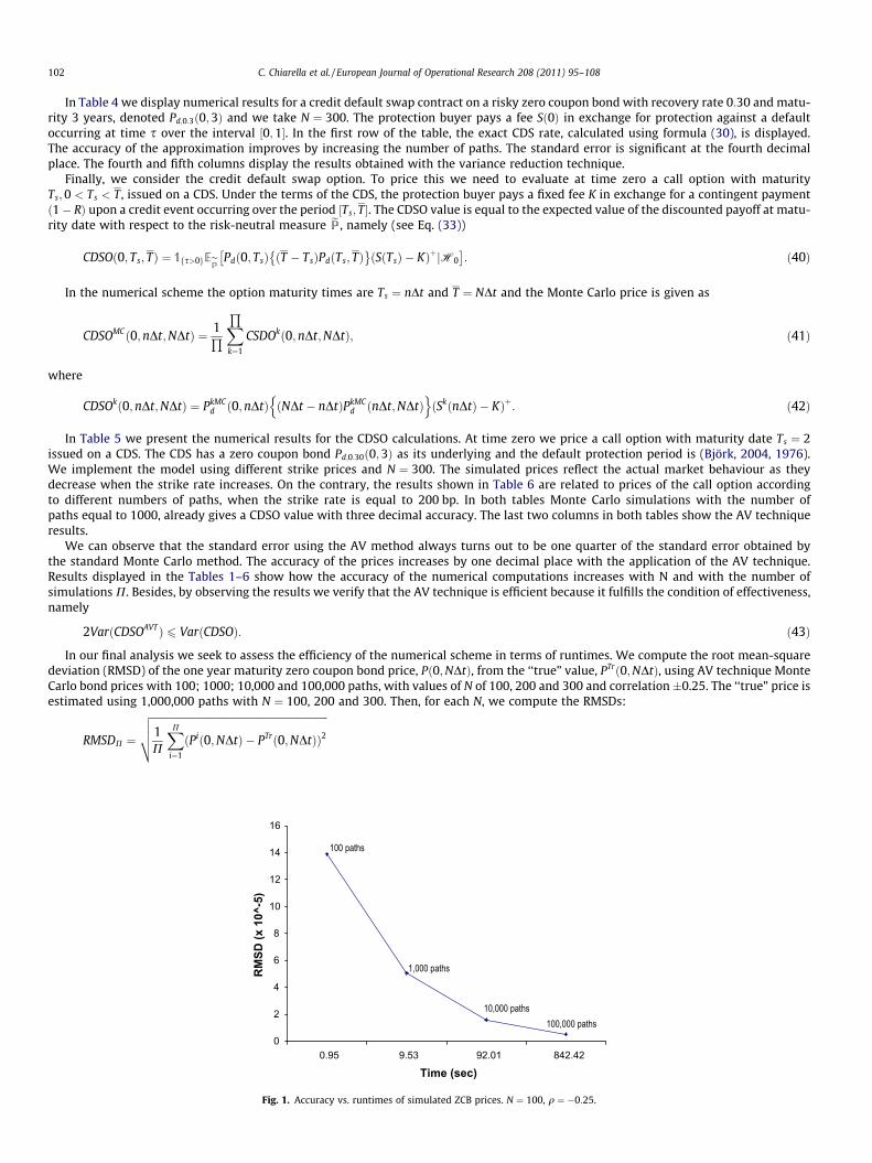
In our final analysis we seek to assess the efficiency of the numerical scheme in terms of runtimes. We compute the root mean-squaredeviation (RMSD) of the one year maturity zero coupon bond price, Pð0;NDtÞ, from the ‘‘true” value, PTrð0;NDtÞ, using AV technique MonteCarlo bond prices with 100; 1000; 10,000 and 100,000 paths, with values of N of 100, 200 and 300 and correlation �0.25. The ‘‘true” price isestimated using 1,000,000 paths with N ¼ 100, 200 and 300. Then, for each N, we compute the RMSDs:

RMSDP ¼

ffiffiffiffiffiffiffiffiffiffiffiffiffiffiffiffiffiffiffiffiffiffiffiffiffiffiffiffiffiffiffiffiffiffiffiffiffiffiffiffiffiffiffiffiffiffiffiffiffiffiffiffiffiffiffiffiffiffiffiffiffiffiffiffiffiffiffiffiffi1P

XPi¼1

ðPið0;NDtÞ � PTrð0;NDtÞÞ2vuut

0

2

4

6

8

10

12

14

16

0.95 9.53 92.01 842.42

Time (sec)

RM

SD (x

10^

-5)

100 paths

1,000 paths

100,000 paths10,000 paths

Fig. 1. Accuracy vs. runtimes of simulated ZCB prices. N ¼ 100, q ¼ �0:25.

0

2

4

6

8

10

12

14

6.95 69.40 693.93 6,998.06

Time (sec)

RM

SD (x

10^

-5)

100 paths

1,000 paths



0

2

4

6

8

10

12

14

16

18

3.40 31.78 316.03 3,813.73

Time (sec)

RM

SD (x

10^

-5)

1,000 paths

100 paths




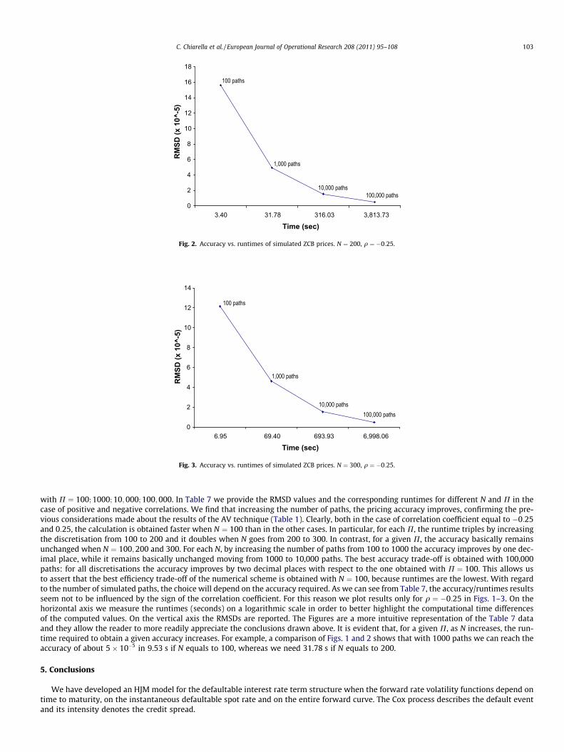
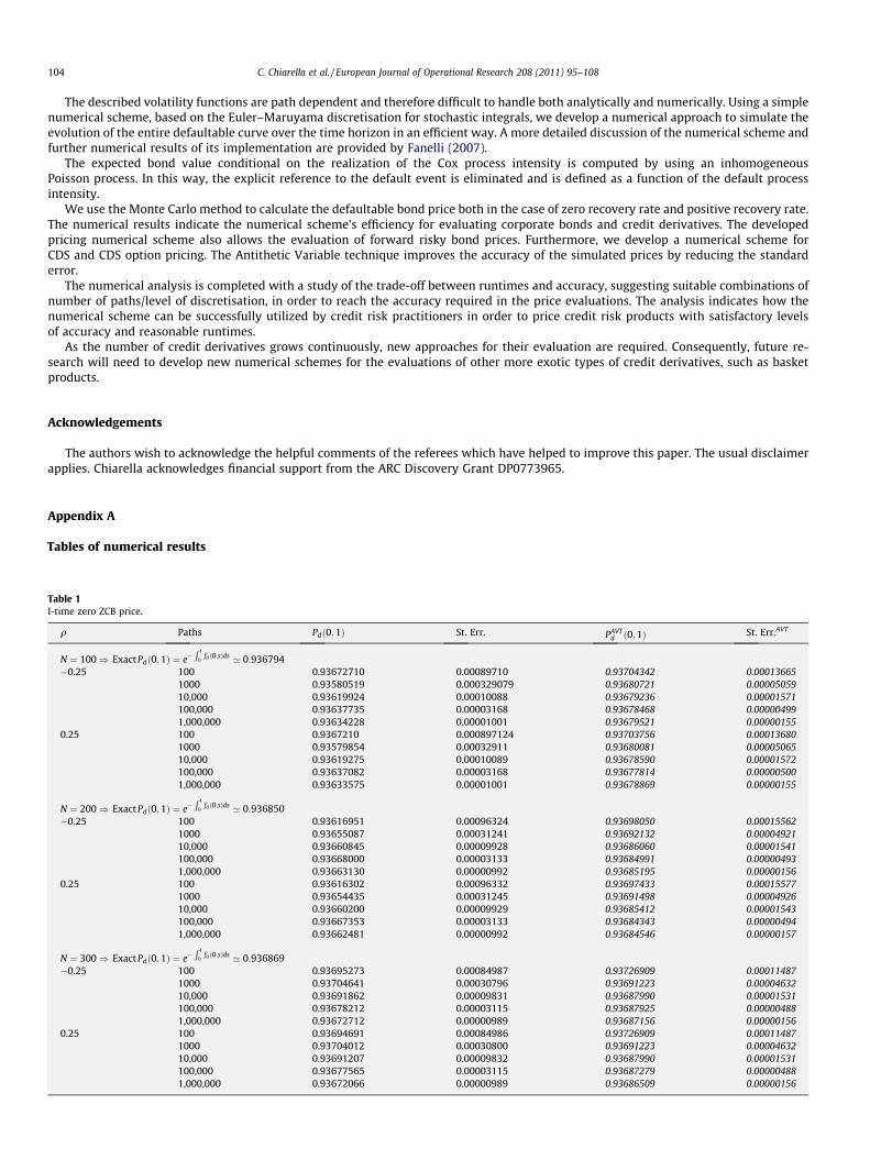
with P ¼ 100; 1000; 10;000; 100;000. In Table 7 we provide the RMSD values and the corresponding runtimes for different N and P in thecase of positive and negative correlations. We find that increasing the number of paths, the pricing accuracy improves, confirming the pre-vious considerations made about the results of the AV technique (Table 1). Clearly, both in the case of correlation coefficient equal to �0:25and 0:25, the calculation is obtained faster when N ¼ 100 than in the other cases. In particular, for each P, the runtime triples by increasingthe discretisation from 100 to 200 and it doubles when N goes from 200 to 300. In contrast, for a given P, the accuracy basically remainsunchanged when N ¼ 100;200 and 300. For each N, by increasing the number of paths from 100 to 1000 the accuracy improves by one dec-imal place, while it remains basically unchanged moving from 1000 to 10,000 paths. The best accuracy trade-off is obtained with 100,000paths: for all discretisations the accuracy improves by two decimal places with respect to the one obtained with P ¼ 100. This allows usto assert that the best efficiency trade-off of the numerical scheme is obtained with N ¼ 100, because runtimes are the lowest. With regardto the number of simulated paths, the choice will depend on the accuracy required. As we can see from Table 7, the accuracy/runtimes resultsseem not to be influenced by the sign of the correlation coefficient. For this reason we plot results only for q ¼ �0:25 in Figs. 1–3. On thehorizontal axis we measure the runtimes (seconds) on a logarithmic scale in order to better highlight the computational time differencesof the computed values. On the vertical axis the RMSDs are reported. The Figures are a more intuitive representation of the Table 7 dataand they allow the reader to more readily appreciate the conclusions drawn above. It is evident that, for a given P, as N increases, the run-time required to obtain a given accuracy increases. For example, a comparison of Figs. 1 and 2 shows that with 1000 paths we can reach theaccuracy of about 5� 10�5 in 9.53 s if N equals to 100, whereas we need 31.78 s if N equals to 200.

5. Conclusions

We have developed an HJM model for the defaultable interest rate term structure when the forward rate volatility functions depend ontime to maturity, on the instantaneous defaultable spot rate and on the entire forward curve. The Cox process describes the default eventand its intensity denotes the credit spread.


The described volatility functions are path dependent and therefore difficult to handle both analytically and numerically. Using a simplenumerical scheme, based on the Euler–Maruyama discretisation for stochastic integrals, we develop a numerical approach to simulate theevolution of the entire defaultable curve over the time horizon in an efficient way. A more detailed discussion of the numerical scheme andfurther numerical results of its implementation are provided by Fanelli (2007).

The expected bond value conditional on the realization of the Cox process intensity is computed by using an inhomogeneousPoisson process. In this way, the explicit reference to the default event is eliminated and is defined as a function of the default processintensity.

We use the Monte Carlo method to calculate the defaultable bond price both in the case of zero recovery rate and positive recovery rate.The numerical results indicate the numerical scheme’s efficiency for evaluating corporate bonds and credit derivatives. The developedpricing numerical scheme also allows the evaluation of forward risky bond prices. Furthermore, we develop a numerical scheme forCDS and CDS option pricing. The Antithetic Variable technique improves the accuracy of the simulated prices by reducing the standarderror.

The numerical analysis is completed with a study of the trade-off between runtimes and accuracy, suggesting suitable combinations ofnumber of paths/level of discretisation, in order to reach the accuracy required in the price evaluations. The analysis indicates how thenumerical scheme can be successfully utilized by credit risk practitioners in order to price credit risk products with satisfactory levelsof accuracy and reasonable runtimes.

As the number of credit derivatives grows continuously, new approaches for their evaluation are required. Consequently, future re-search will need to develop new numerical schemes for the evaluations of other more exotic types of credit derivatives, such as basketproducts.

Acknowledgements

The authors wish to acknowledge the helpful comments of the referees which have helped to improve this paper. The usual disclaimerapplies. Chiarella acknowledges financial support from the ARC Discovery Grant DP0773965.

Appendix A

Tables of numerical results

Table 1I-time zero ZCB price.

q Paths Pdð0;1Þ St. Err. PAVTd ð0;1Þ St. Err.AVT

N ¼ 100) ExactPdð0;1Þ ¼ e�R 1

0fdð0;sÞds ’ 0:936794

�0.25 100 0.93672710 0.00089710 0.93704342 0.000136651000 0.93580519 0.000329079 0.93680721 0.0000505910,000 0.93619924 0.00010088 0.93679236 0.00001571100,000 0.93637735 0.00003168 0.93678468 0.000004991,000,000 0.93634228 0.00001001 0.93679521 0.00000155

0.25 100 0.9367210 0.000897124 0.93703756 0.000136801000 0.93579854 0.00032911 0.93680081 0.0000506510,000 0.93619275 0.00010089 0.93678590 0.00001572100,000 0.93637082 0.00003168 0.93677814 0.000005001,000,000 0.93633575 0.00001001 0.93678869 0.00000155


0fdð0;sÞds ’ 0:936850

�0.25 100 0.93616951 0.00096324 0.93698050 0.000155621000 0.93655087 0.00031241 0.93692132 0.0000492110,000 0.93660845 0.00009928 0.93686060 0.00001541100,000 0.93668000 0.00003133 0.93684991 0.000004931,000,000 0.93663130 0.00000992 0.93685195 0.00000156

0.25 100 0.93616302 0.00096332 0.93697433 0.000155771000 0.93654435 0.00031245 0.93691498 0.0000492610,000 0.93660200 0.00009929 0.93685412 0.00001543100,000 0.93667353 0.00003133 0.93684343 0.000004941,000,000 0.93662481 0.00000992 0.93684546 0.00000157


0fdð0;sÞds ’ 0:936869

�0.25 100 0.93695273 0.00084987 0.93726909 0.000114871000 0.93704641 0.00030796 0.93691223 0.0000463210,000 0.93691862 0.00009831 0.93687990 0.00001531100,000 0.93678212 0.00003115 0.93687925 0.000004881,000,000 0.93672712 0.00000989 0.93687156 0.00000156

0.25 100 0.93694691 0.00084986 0.93726909 0.000114871000 0.93704012 0.00030800 0.93691223 0.0000463210,000 0.93691207 0.00009832 0.93687990 0.00001531100,000 0.93677565 0.00003115 0.93687279 0.000004881,000,000 0.93672066 0.00000989 0.93686509 0.00000156

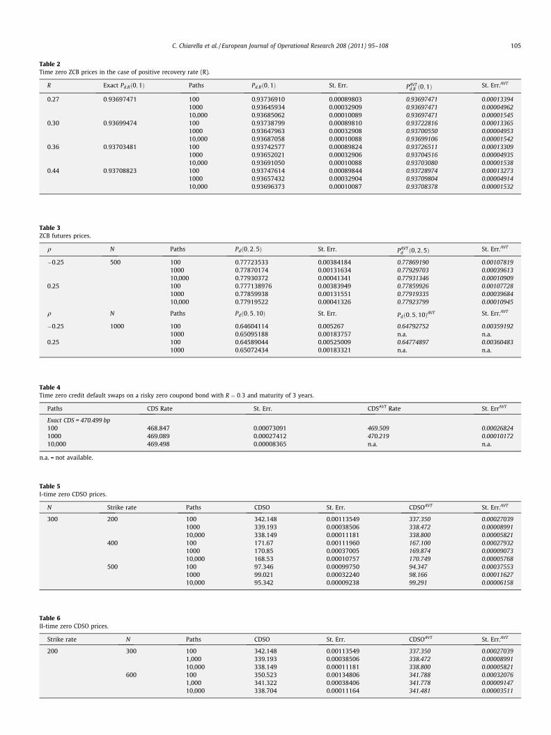
Table 5I-time zero CDSO prices.

N Strike rate Paths CDSO St. Err. CDSOAVT St. Err.AVT

300 200 100 342.148 0.00113549 337.350 0.000270391000 339.193 0.00038506 338.472 0.0000899110,000 338.149 0.00011181 338.800 0.00005821

400 100 171.67 0.00111960 167.100 0.000279321000 170.85 0.00037005 169.874 0.0000907310,000 168.53 0.00010757 170.749 0.00005768

500 100 97.346 0.00099750 94.347 0.000375531000 99.021 0.00032240 98.166 0.0001162710,000 95.342 0.00009238 99.291 0.00006158

Table 3ZCB futures prices.

q N Paths Pdð0;2;5Þ St. Err. PAVTd ð0;2;5Þ St. Err.AVT

�0.25 500 100 0.77723533 0.00384184 0.77869190 0.001078191000 0.77870174 0.00131634 0.77929703 0.0003961310,000 0.77930372 0.00041341 0.77931346 0.00010909

0.25 100 0.777138976 0.00383949 0.77859926 0.001077281000 0.77859938 0.00131551 0.77919335 0.0003968410,000 0.77919522 0.00041326 0.77923799 0.00010945

q N Paths Pdð0;5;10Þ St. Err. Pdð0;5;10ÞAVT St. Err.AVT

�0.25 1000 100 0.64604114 0.005267 0.64792752 0.003591921000 0.65095188 0.00183757 n.a. n.a.

0.25 100 0.64589044 0.00525009 0.64774897 0.003604831000 0.65072434 0.00183321 n.a. n.a.

Table 4Time zero credit default swaps on a risky zero coupond bond with R ¼ 0:3 and maturity of 3 years.

Paths CDS Rate St. Err. CDSAVT Rate St. ErrAVT

Exact CDS = 470.499 bp100 468.847 0.00073091 469.509 0.000268241000 469.089 0.00027412 470.219 0.0001017210,000 469.498 0.00008365 n.a. n.a.

n.a. = not available.

Table 6II-time zero CDSO prices.

Strike rate N Paths CDSO St. Err. CDSOAVT St. Err.AVT

200 300 100 342.148 0.00113549 337.350 0.000270391,000 339.193 0.00038506 338.472 0.0000899110,000 338.149 0.00011181 338.800 0.00005821

600 100 350.523 0.00134806 341.788 0.000320761,000 341.322 0.00038406 341.778 0.0000914710,000 338.704 0.00011164 341.481 0.00003511

Table 2Time zero ZCB prices in the case of positive recovery rate (R).

R Exact Pd;Rð0;1Þ Paths Pd;Rð0;1Þ St. Err. PAVTd;R ð0;1Þ St. Err.AVT

0.27 0:93697471 100 0.93736910 0.00089803 0.93697471 0.000133941000 0.93645934 0.00032909 0.93697471 0.0000496210,000 0.93685062 0.00010089 0.93697471 0.00001545

0.30 0:93699474 100 0.93738799 0.00089810 0.93722816 0.000133651000 0.93647963 0.00032908 0.93700550 0.0000495310,000 0.93687058 0.00010088 0.93699106 0.00001542

0.36 0:93703481 100 0.93742577 0.00089824 0.93726511 0.000133091000 0.93652021 0.00032906 0.93704516 0.0000493510,000 0.93691050 0.00010088 0.93703080 0.00001538

0.44 0:93708823 100 0.93747614 0.00089844 0.93728974 0.000132731000 0.93657432 0.00032904 0.93709804 0.0000491410,000 0.93696373 0.00010087 0.93708378 0.00001532


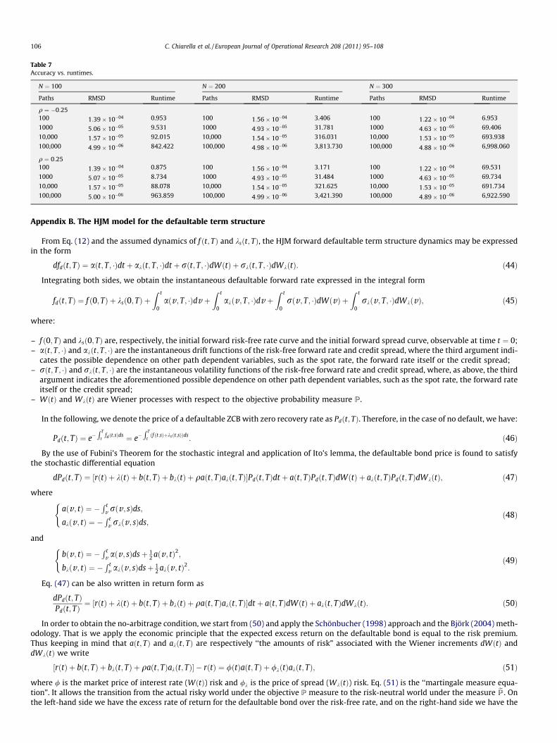
Table 7Accuracy vs. runtimes.

N ¼ 100 N ¼ 200 N ¼ 300

Paths RMSD Runtime Paths RMSD Runtime Paths RMSD Runtime

q ¼ �0:25100 1:39� 10�04 0.953 100 1:56� 10�04 3.406 100 1:22� 10�04 6.953

1000 5:06� 10�05 9.531 1000 4:93� 10�05 31.781 1000 4:63� 10�05 69.406

10,000 1:57� 10�05 92.015 10,000 1:54� 10�05 316.031 10,000 1:53� 10�05 693.938

100,000 4:99� 10�06 842.422 100,000 4:98� 10�06 3,813.730 100,000 4:88� 10�06 6,998.060

q ¼ 0:25100 1:39� 10�04 0.875 100 1:56� 10�04 3.171 100 1:22� 10�04 69.531

1000 5:07� 10�05 8.734 1000 4:93� 10�05 31.484 1000 4:63� 10�05 69.734

10,000 1:57� 10�05 88.078 10,000 1:54� 10�05 321.625 10,000 1:53� 10�05 691.734

100,000 5:00� 10�06 963.859 100,000 4:99� 10�06 3,421.390 100,000 4:89� 10�06 6,922.590


Appendix B. The HJM model for the defaultable term structure

From Eq. (12) and the assumed dynamics of f ðt; TÞ and ksðt; TÞ, the HJM forward defaultable term structure dynamics may be expressedin the form

dfdðt; TÞ ¼ aðt; T; �Þdt þ akðt; T; �Þdt þ rðt; T; �ÞdWðtÞ þ rkðt; T; �ÞdWkðtÞ: ð44Þ

Integrating both sides, we obtain the instantaneous defaultable forward rate expressed in the integral form

fdðt; TÞ ¼ f ð0; TÞ þ ksð0; TÞ þZ t

0aðv; T; �Þdv þ

Z t

0akðv ; T; �Þdv þ

Z t

0rðv; T; �ÞdWðvÞ þ

Z t

0rkðv; T; �ÞdWkðvÞ; ð45Þ

where:

– f ð0; TÞ and ksð0; TÞ are, respectively, the initial forward risk-free rate curve and the initial forward spread curve, observable at time t ¼ 0;– aðt; T; �Þ and akðt; T; �Þ are the instantaneous drift functions of the risk-free forward rate and credit spread, where the third argument indi-

cates the possible dependence on other path dependent variables, such as the spot rate, the forward rate itself or the credit spread;– rðt; T; �Þ and rkðt; T; �Þ are the instantaneous volatility functions of the risk-free forward rate and credit spread, where, as above, the third

argument indicates the aforementioned possible dependence on other path dependent variables, such as the spot rate, the forward rateitself or the credit spread;

– WðtÞ and WkðtÞ are Wiener processes with respect to the objective probability measure P.

In the following, we denote the price of a defaultable ZCB with zero recovery rate as Pdðt; TÞ. Therefore, in the case of no default, we have:

Pdðt; TÞ ¼ e�R T

tfdðt;sÞds ¼ e�

R T

tðf ðt;sÞþksðt;sÞÞds

: ð46Þ

By the use of Fubini’s Theorem for the stochastic integral and application of Ito’s lemma, the defaultable bond price is found to satisfythe stochastic differential equation

dPdðt; TÞ ¼ ½rðtÞ þ kðtÞ þ bðt; TÞ þ bkðtÞ þ qaðt; TÞakðt; TÞ�Pdðt; TÞdt þ aðt; TÞPdðt; TÞdWðtÞ þ akðt; TÞPdðt; TÞdWkðtÞ; ð47Þ

where

aðv ; tÞ ¼ �R t

v rðv ; sÞds;

akðv ; tÞ ¼ �R t

v rkðv ; sÞds;

(ð48Þ

and

bðv; tÞ ¼ �R t

v aðv ; sÞdsþ 12 aðv ; tÞ2;

bkðv ; tÞ ¼ �R t

v akðv ; sÞdsþ 12 akðv; tÞ2:

(ð49Þ

Eq. (47) can be also written in return form as

dPdðt; TÞPdðt; TÞ

¼ ½rðtÞ þ kðtÞ þ bðt; TÞ þ bkðtÞ þ qaðt; TÞakðt; TÞ�dt þ aðt; TÞdWðtÞ þ akðt; TÞdWkðtÞ: ð50Þ

In order to obtain the no-arbitrage condition, we start from (50) and apply the Schönbucher (1998) approach and the Björk (2004) meth-odology. That is we apply the economic principle that the expected excess return on the defaultable bond is equal to the risk premium.Thus keeping in mind that aðt; TÞ and akðt; TÞ are respectively ‘‘the amounts of risk” associated with the Wiener increments dWðtÞ anddWkðtÞ we write

½rðtÞ þ bðt; TÞ þ bkðt; TÞ þ qaðt; TÞakðt; TÞ� � rðtÞ ¼ /ðtÞaðt; TÞ þ /kðtÞakðt; TÞ; ð51Þ

where / is the market price of interest rate (WðtÞ) risk and /k is the price of spread (WkðtÞ) risk. Eq. (51) is the ‘‘martingale measure equa-tion”. It allows the transition from the actual risky world under the objective P measure to the risk-neutral world under the measure eP. Onthe left-hand side we have the excess rate of return for the defaultable bond over the risk-free rate, and on the right-hand side we have the


linear combination of the volatilities and market prices of risk that combine to yield the instantaneous risk premium. Some simple rearrange-ments express (51) in the more convenient form

bðt; TÞ � /ðtÞaðt; TÞ þ bkðt; TÞ � /kðtÞakðt; TÞ þ qaðt; TÞakðt; TÞ ¼ 0: ð52Þ

By substituting (48) and (49) into (52) we obtain

�Z T

taðt; sÞdsþ 1

2

Z T

trðt; sÞds

� �2

�Z T

takðt; sÞdsþ 1

2

Z T

trkðt; sÞds

� �2

þ qZ T

trðt; sÞds

Z T

trkðt; sÞds

þ /ðtÞZ T

trðt; sÞdsþ /kðtÞ

Z T

trkðt; sÞds ¼ 0: ð53Þ

By differentiating with respect to T, the above expression can be rewritten in the form

� aðt; TÞ þ rðt; TÞZ T

trðt; sÞds� akðt; TÞ þ rkðt; TÞ

Z T

trkðt; sÞdsþ qrðt; TÞ

Z T

trkðt; sÞds

þ qrkðt; TÞZ T

trðt; sÞds� /ðtÞrðt; TÞ � /kðtÞrkðt; TÞ ¼ 0: ð54Þ

From (54) we can obtain the HJM forward rate drift restriction for defaultable processes, namely

adðt; TÞ ¼ aðt; TÞ þ akðt; TÞ ¼ rðt; TÞZ T

trðt; sÞdsþ rkðt; TÞ

Z T

trkðt; sÞds

þ q rðt; TÞZ T


Z T

trðt; sÞds

� �0 � /ðtÞrðt; TÞ � /kðtÞrkðt; TÞ: ð55Þ

We define two new processes

fW ðtÞ ¼WðtÞ þZ t

0ð�/ðsÞÞds; ð56Þ

and

fW kðtÞ ¼WkðtÞ þZ t

0ð�/kðsÞÞds; ð57Þ

so that

dfW ðtÞ ¼ dWðtÞ � /ðtÞdt; ð58Þ

and

dfW kðtÞ ¼ dWkðtÞ � /kðtÞdt: ð59Þ

For later calculations we note that the last two equations imply that

dWðtÞ ¼ dfW ðtÞ þ /ðtÞdt; ð60Þ
and
dWkðtÞ ¼ dfW kðtÞ þ /kðtÞdt: ð61Þ

By an application of Girsanov’s Theorem fW ðtÞ and fW kðtÞ will be Wiener processes under eP. By substituting (55), (60) and (61) into (44)we obtain

dfdðt; TÞ ¼ rðt; TÞZ T

trðt; sÞdsþ rkðt; TÞ

Z T

trkðt; sÞdsþ qrðt; TÞ

Z T

trkðt; sÞdsþ qrkðt; TÞ

Z T

trðt; sÞds

� �dt þ rðt; TÞdfW ðtÞ

þ rkðt; TÞdfW kðtÞ: ð62Þ

By integrating, we obtain the instantaneous defaultable forward rate dynamics in stochastic integral equation form, namely

fdðt; TÞ ¼ f ð0; TÞ þ ksð0; TÞ0 þZ t

0rðv; TÞ

Z T

vrðv; sÞdsþ rkðv ; TÞ

Z T

vrkðv ; sÞds

� �dv

þZ t

0q rðv ; TÞ

Z T

vrkðv; sÞdsþ rkðv ; TÞ

Z T

vrðv ; sÞds

� �dv þ

Z t

0rðv ; TÞdfW ðvÞ þ rkðv; TÞdfW kðvÞh i

: ð63Þ

From (63) we derive the defaultable spot rate process rdðtÞ ¼ fdðt; tÞ, so that

rdðtÞ ¼ f ð0; tÞ þ ksð0; tÞ þZ t

0rðv ; tÞ

Z t

vrðv ; sÞdsþ rkðv; tÞ

Z t

vrkðv ; sÞds

� �dv

þZ t

0q rðv; tÞ

Z t

vrkðv; sÞdsþ rkðv; tÞ

Z t

vrðv ; sÞds

� �dv þ

Z t

0rðv ; tÞdfW ðvÞ þ rkðv; tÞdfW kðvÞh i

: ð64Þ

From (55) and (5) we deduce the HJM credit spread drift condition, which can be written

akðt; TÞ ¼ q rðt; TÞZ T


Z T

trðt; sÞds

� �þ rkðt; TÞ

Z T

trkðt; sÞds� /kðtÞrkðt; TÞ: ð65Þ


As in the default free HJM model, the derivative security price is evaluated independently of the market prices of risk, because they getabsorbed in the change of measure to eP, under which the spot rate and bond price processes are expressed in the arbitrage-free dynamics.Finally we derive the bond pricing formula under eP.

We start by choosing the numeraire

BdðtÞ ¼ eR t

0rdðsÞds

;

so that relative bond price is given by

Zðt; TÞ ¼ Pdðt; TÞBdðtÞ

¼ Pdðt; TÞe�R t

0rdðtÞds

: ð66Þ

By applying Ito’s Lemma to (66) and recalling the definitions (48) and (49), we obtain

dZðt; TÞ ¼ bðt; TÞZðt; TÞ þ bkðt; TÞZðt; TÞ½ �dt þ aðt; TÞZðt; TÞdW þ akðt; TÞZðt; TÞdWk: ð67Þ

By Girsanov’s Theorem and using relation (52), the process (67) can be written in terms of the Brownian motions (58) and (59) gener-ated by the equivalent martingale probability measure eP, thus we write

dZðt; TÞ ¼ aðt; TÞZðt; TÞdfW ðtÞ þ akðt; TÞZðt; TÞdfW kðtÞ: ð68Þ

Since the stochastic differential equation is driftless, Zðt; TÞ is a martingale under the probability measure eP and the bond value is cal-culated as the expected value with respect to the probability measure eP with expected future payoffs discounted using the defaultable raterdðtÞ, that is

Pdðt; TÞ ¼ EeP e�R t

trdðsÞds

� �: ð69Þ

The above evaluation rule may be applied to price any derivative security within the HJM framework. An exhaustive mathematicalexplanation of the risk-neutral valuation principle is given in Bielecki and Rutkowski (2001).

References

Bielecki, T., Rutkowski, M., 2001. Credit risk: modeling. Valuation and Hedging. Springer-Verlag.Björk, T., 2004. Arbitrage Theory in Continuous Time, second ed. OXFORD Finance.Black, F., Cox, J., 1976. Valuing Corporate securities: some effects of bond indenture provisions. Journal of Finance 31 (2), 351–367.Brigo, D., Morini, M., 2005. CDS market formulas and models. In: Proceedings of the 18th Annual Warwick Options Conference, September 30, 2005, Warwick, UK.Chen, R., Cheng, X., Fabozzi, F.J., Liu, B., 2008. An explicit, multi-factor credit default swap pricing model with correlated factors. Journal of Financial and Quantitative Analysis

43 (1), 123–160.Chiarella, C., Clewlow, L., Musti, S., 2005. A volatility decomposition control variate technique for Monte Carlo simulations of Heath Jarrow Morton models. European Journal

of Operational Research 161 (2), 325–336.Cox, J., Ingersoll, J., Ross, S., 1985. A theory of the term structure of interest rates. Econometrica 53, 385–407.Das, S., Sundaram, R., 2000. A discrete-time approach to arbitrage-free pricing of credit derivatives. Management Science 46 (1), 46–62.Duffie, D., Lando, D., 2001. Term structures of credit spreads with incomplete accounting information. Econometrica 69, 633–664.Duffie, D., Singleton, K., 1999. Modelling term structures of defaultable bonds. Review of Financial Studies 12, 687–720.Fanelli, V. (2007). Numerical implementation of a credit risk model in the HJM framework. Ph.D. Thesis, Dipartimento di Scienze Economiche, Matematiche e Statistiche,

Universitdi Foggia.Heath, D., Jarrow, R., Morton, A., 1992. Bond pricing and the term structure of interest rates: a new methodology for contingent claims valuation. Econometrica 60 (1), 77–105.Hull, J., White, A., 2000. Valuing credit default swaps I: no counterparty default risk. Journal of Derivatives 8 (1), 29–40.Hull, J., White, A., 2001. Valuing credit default swaps II: modeling default correlations. Journal of Derivatives 8 (3), 12–22.Jamshidian, F., 2004. Valuation of credit default swaps and swaptions. Finance and Stochastics 8 (3), 343–371.Jarrow, R., Lando, D., Turnbull, S., 1997. A Markov model for the term structure of credit spreads. Review of Financial Studies 10, 481–523.Jarrow, R.A., Turnbull, S.M., 1995. Pricing derivatives on financial securities subject to credit risk. Journal of Finance 50 (1), 53–85.Jeanblanc, M., Rutkowski, M., 2002. Default risk and hazard process. In: Geman, H., Madan, D., Pliska, S.R., Vorst, T. (Eds.), Mathematical Finance-Bachelier Congress 2000,

Springer-Verlag, Berlin, pp. 281–312.Kloeden, P., Platen, E., 1999. Numerical Solution of Stochastic Differential Equations. Springer-Verlag.Lando, D., 1998. On Cox processes and credit risky securities. Review of Derivatives Research 2 (2/3), 99–120.Longstaff, F., Schwartz, E., 1995. The pricing of credit risk derivatives. Journal of Fixed Income 5 (1), 6–14.Maksyumiuk, R., Gtarek, D., 1999. Applying HJM to credit risk. Risk 12 (5), 67–68.Merton, R., 1974. On the pricing of corporate debt: the risk structure of interest rates. Journal of Finance 29, 449–470.Moody’s Investors Service, 2007. European Corporate Default and Recovery Rates, 1982–2006.Pugachevsky, D., 1999. Generalizing with HJM. Risk 12, 103–105.Schönbucher, P., 1996. Valuation of securities subject to credit risk, University of Bonn, Department of Statistics, retrieved May 10, 2006, from <http://www.schonbucher.de>.Schönbucher, P., 1998. Term structure modelling of defaultable bonds. Review of Derivatives Research 2, 123–134.Shimko, D., Tejima, N., Deventer, D., 1993. The pricing of risky debt when interest rates are stochastic. Journal of Fixed Income, 58–66.Zhou, C., 1997. Jump-diffusion approach to modeling credit risk and valuing defaultable securities, Finance and Economics Discussion Paper Series 1997/15, Board of

Governors of the Federal Reserve System.

http://www.schonbucher.de

Documents

Modelling the evolution of credit spreads using the Cox process within the HJM framework: A CDS option pricing model