Modelling the cost-effectiveness of primary hip

CENTRE FOR HEALTH ECONOMICS

Modelling the cost-effectiveness of primary hip replacement: how cost-effective is the Spectron

compared to the Charnley prosthesis?

Andrew Briggs Mark Sculpher

Jill Dawson Ray Fitzpatrick David Murray

Henrik Malchau

CHE Technical Paper Series 28

2

CENTRE FOR HEALTH ECONOMICS TECHNICAL PAPER SERIES The Centre for Health Economics has a well established Discussion Paper series which was originally conceived as a means of circulating ideas for discussion and debate amongst a wide readership that included health economists as well as those working within the NHS and pharmaceutical industry. The introduction of a Technical Paper Series offers a further means by which the Centre’s research can be disseminated. The Technical Paper Series publishes papers that are likely to be of specific interest to a relatively specialist audience, for example papers dealing with complex issues that assume high levels of prior knowledge, or those that make extensive use of sophisticated mathematical or statistical techniques. The content and its format are entirely the responsibility of the author, and papers published in the Technical Paper series are not subject to peer-review or editorial control, unlike those produced in the Discussion Paper series. Offers of further papers, and requests for information should be directed to Frances Sharp in the Publications Office, Centre for Health Economics, University of York.

December 2003. © Andrew Briggs,, Mark Sculpher, Jill Dawson, Ray Fitzpatrick, David Murray, Henrik Malchau

3

Modelling the cost-effectiveness of primary hip replacement: how cost-effective is the Spectron compared to the Charnley prosthesis?

Technical Report

Andrew Briggs1

Mark Sculpher2

Jill Dawson3

Ray Fitzpatrick4

David Murray5

Henrik Malchau6

1. Health Economics Research Centre, University of Oxford, Institute for

Health Sciences, Headington, Oxford OX3 7LF, UK

2. Centre for Health Economics, University of York, Heslington, York YO10

5DD, UK

3. School of Health Care, Oxford Brookes University, 44 London Road,

Oxford OX3 7PD, UK

4. Department of Public Health, University of Oxford, Institute for Health

Sciences, Headington, Oxford OX3 7LF, UK

5. Nuffield Orthopaedic Centre, Headington, Oxford OX3 7LD, UK

6. Department of Orthopedics, Institute of Surgical Sciences, Sahlgrenska

University Hospital, Göteborg University, S-413 45 Göteborg, Sweden

4

Preamble The purpose of this Technical Report is to describe the development of a fully probabilistic cost-effectiveness model of primary hip replacement. This development is built upon the structure of a previously reported cost-effectiveness model presented as part of a general Health Technology Assessment report on the Hip Prostheses. The new model retains the same (Markov) structure of the original, but is updated to a fully probabilistic model from available data sources. Evidence on long-term failure rates of the Spectron prosthesis (an example of a modern cemented prosthesis) compared to the Charnley prosthesis (the most commonly used prosthetic device in the UK) was obtained from the Swedish National Hip Arthroplasty Register – one of the largest registries of hip prosthesis use in the world. Information on quality of life for patients undergoing hip replacement surgery was obtained from a study of patients at the Nuffield Orthopaedic Centre in Oxford, who were given EQ-5D questionnaires immediately prior to and 12 months following hip replacement surgery. These two patient level data sources allow statistical estimation of the distribution of the associated model parameters together with their covariance structure. Cost data on the prostheses themselves were obtained from the manufacturers and cost data for revision operations were obtained from published NHS reference costs. Mortality rates were obtained from published life-tables. Distributions for the remaining model parameters were obtained from the literature. A particular feature of the model was the ability to estimate cost-effectiveness by age and sex of the patient, since it is well established that age and sex have an important effect on the risk of revision.

5

1 Introduction The effectiveness and cost-effectiveness of primary total hip replacement (THR) has been established,1,2 at least in some patient groups, and approximately 50,000 procedures are now undertaken annually in the UK.3 However, there is less clarity regarding the cost-effectiveness of alternative prostheses. A range of prostheses is available for THR, with considerable variation in acquisition cost.4 The Charnley THR is generally considered to be the ‘gold standard’ and is one of the cheapest implants available. There are now available, however, a number of new designs and modifications of old designs that may have better results that the Charnley but are more expensive. In order for these new, more expensive, prostheses to show their cost-effectiveness relative to the Charnley, they must be able to show a reduced failure rate sufficient to generate meaningful gains in quality-adjusted life expectancy and/or cost savings from lower rates of revision surgery. In 2000, the National Institute for Clinical Excellence in the UK reviewed available evidence on the effectiveness and cost-effectiveness of alternative hip prostheses.5NICE concluded that prostheses should only be used in the NHS if they are able to demonstrate, using appropriate trial or observational data, 10-year revision rates of 10% or less, or rates consistent with that over a shorter period of not less than 3 years. NICE’s guidance also made clear the dearth of effectiveness data from appropriately powered randomised trials with sufficient follow-up to assess long-term revision rates. The Institute recognised that data on long-term revision rates would typically have to be identified in non-experimental studies, such as national registers. The Swedish National Total Hip Arthroplasty Register was started in 1979, and is one of the most established sources of data of this sort.6 It covers all hospitals in Sweden, and now includes over 205,000 hip arthroplasties. In order to use these data on the revision rates associated with alternative prostheses to establish their comparative cost-effectiveness, it is necessary to bring to bear additional data inputs such as the prices of the prostheses, the mortality rate associated with hip replacement and the underlying rate in relevant populations, the health-related quality of life implications of the failure of a primary arthroplasty and the cost

6

of a revision operation. In order to synthesis these and other data, decision analytic modelling provides a crucial role. These are mathematical expressions of the treatment pathways and prognoses that patients may experience consequent on alternative interventions. They facilitate estimates of differential effectiveness and cost-effectiveness recognising the uncertainty associated with data inputs introduced into the model. Decision analytic models have been developed which can assess the cost-effectiveness of hip replacement in general,2 and of alternative hip prostheses.7-9

In 1996, we developed a cost-effectiveness model to provide a general framework for assessing the cost-effectiveness of alternative hip prostheses.9 This subsequently provided one source of information upon which NICE’s guidance was based.5 In this paper, we report on the further development of this model. In the Swedish National Total Hip Arthroplasty Register there are a number of cemented THRs which may have better survival rates than the Charnley. These include the Lubinus SPII, the Exeter Polished, the Scan Hip and the Spectron EF. To explore the cost-effectiveness of these, we have compared the Charnley with the Spectron.

2 Model Structure The analysis is based on a simple Markov process, which is a form of decision analytic model used widely in health services research, and in economic evaluation in particular. A Markov model involves dividing a patient’s possible prognoses into a series of health states. The probabilities defining transition between each of these states are specified over a particular time frame (a ‘cycle’) such as a month or a year. With the aid of a computer, the model is run over a large number of cycles to see how a hypothetical cohort of patients would move between states. Different probabilities are defined for each form of management under evaluation and the costs and benefits of the comparators are estimated on the basis of the length of time the cohort of patients spends in each state. The Markov model is employed to predict the prognosis of patients who have undergone primary THR. Following the operation, patients are assumed to enter the Markov model, which consists of four distinct states:

7

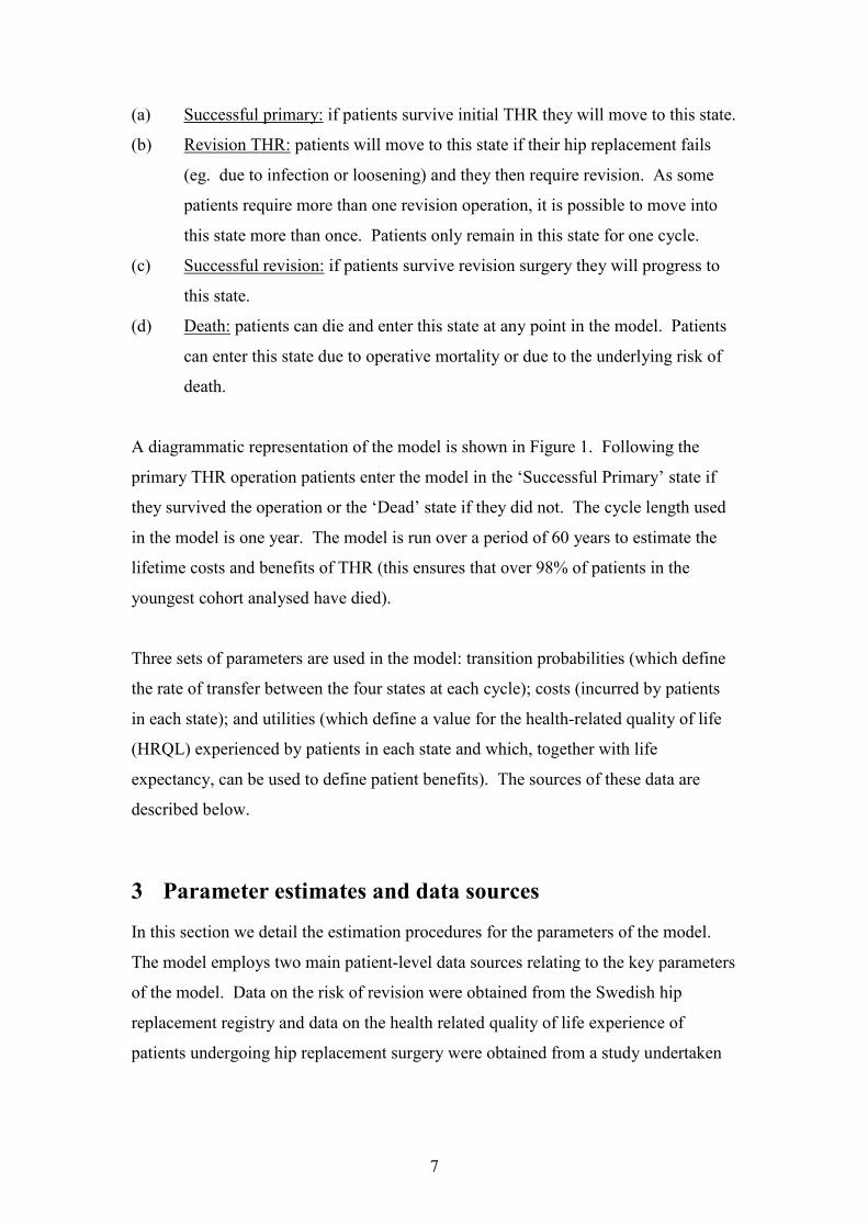
(a) Successful primary: if patients survive initial THR they will move to this state. (b) Revision THR: patients will move to this state if their hip replacement fails

(eg. due to infection or loosening) and they then require revision. As some patients require more than one revision operation, it is possible to move into this state more than once. Patients only remain in this state for one cycle.

(c) Successful revision: if patients survive revision surgery they will progress to this state.

(d) Death: patients can die and enter this state at any point in the model. Patients can enter this state due to operative mortality or due to the underlying risk of death.

A diagrammatic representation of the model is shown in Figure 1. Following the primary THR operation patients enter the model in the ‘Successful Primary’ state if they survived the operation or the ‘Dead’ state if they did not. The cycle length used in the model is one year. The model is run over a period of 60 years to estimate the lifetime costs and benefits of THR (this ensures that over 98% of patients in the youngest cohort analysed have died). Three sets of parameters are used in the model: transition probabilities (which define the rate of transfer between the four states at each cycle); costs (incurred by patients in each state); and utilities (which define a value for the health-related quality of life (HRQL) experienced by patients in each state and which, together with life expectancy, can be used to define patient benefits). The sources of these data are described below.

3 Parameter estimates and data sources In this section we detail the estimation procedures for the parameters of the model. The model employs two main patient-level data sources relating to the key parameters of the model. Data on the risk of revision were obtained from the Swedish hip replacement registry and data on the health related quality of life experience of patients undergoing hip replacement surgery were obtained from a study undertaken

8

in the UK. Other parameter estimates required to populate the model were obtained from the literature.

3.1 Revision risks: evidence from the Swedish Register The Swedish National Hip Arthroplasty Register contains records of all hip replacement operations performed in Sweden. We obtained data from the registry of all patients receiving either a Charnley or Spectron primary hip replacement in the period 1992-2000. This period was chosen since it is the period within which both the current manifestations of the Charnley and Spectron prostheses have been approximately constant. Only data where both the cup and stem from the same manufacturer had been used (less than 1% of cases had used unmatched cup and stem) were included. For the Spectron, all patients having an All-Poly Cup and a Spectron EF or EF Primary Stem (Smith and Nephew, Memphis, Tenn, USA) were used. The final data set employed contained data on 20,495 patients undergoing a primary hip replacement: 18,505 (90%) of these received the Charnley prosthesis and the remaining 1,990 (10%) received the Spectron. The mean follow up period was 4 years 3 months with a maximum follow up of just over eight years. This gave a total of almost 90,000 patient years at risk, during which 574 failures were observed. The purpose of this section is to describe the approach taken to estimating the risk of revision from the Swedish Registry data. We begin with simple non-parametric methods; we go on to consider an appropriate parametric form of the hazard function; and finally we consider the use of dual hazard functions to generate a ‘bathtub’ failure curve for extrapolation.

3.1.1 Initial nonparametric survival analysis The data from the Swedish Registry represent time to event information, with the event in this case being the failure of the prosthesis (defined by the need for revision). Since the time period is relatively short (median follow-up four years, max eight years) and the need for revision relatively rare, many patients in the data set do not have the event of interest. This represents right censoring of the data and standard survival analysis techniques can be employed to handle this issue. Perhaps the most commonly employed method for handling survival data of this kind is the non-

9

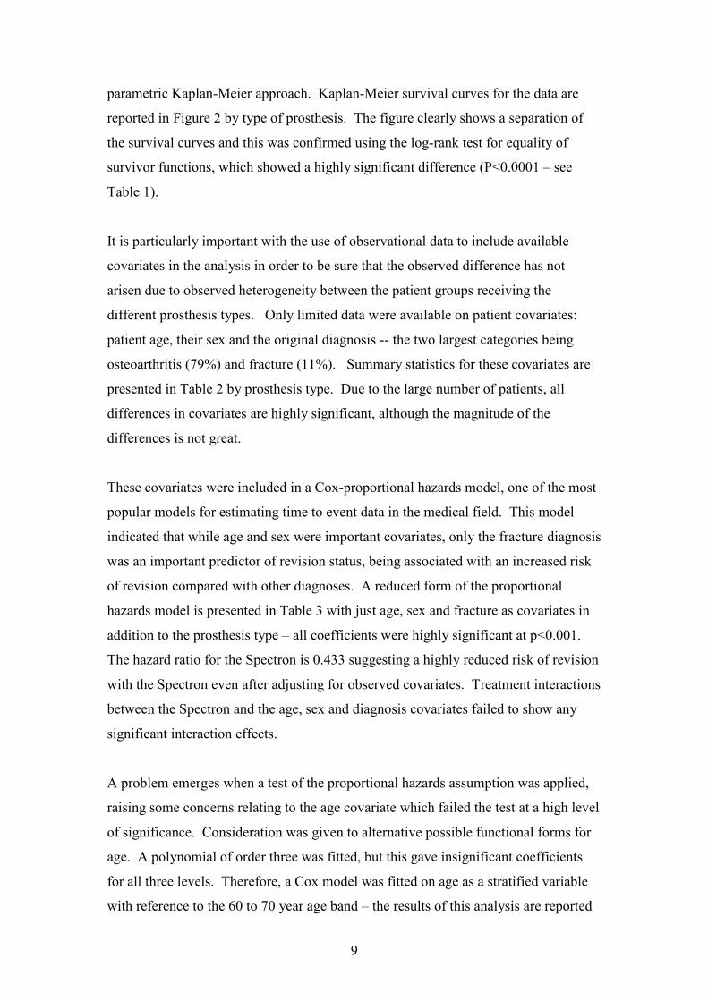
parametric Kaplan-Meier approach. Kaplan-Meier survival curves for the data are reported in Figure 2 by type of prosthesis. The figure clearly shows a separation of the survival curves and this was confirmed using the log-rank test for equality of survivor functions, which showed a highly significant difference (P<0.0001 – see Table 1). It is particularly important with the use of observational data to include available covariates in the analysis in order to be sure that the observed difference has not arisen due to observed heterogeneity between the patient groups receiving the different prosthesis types. Only limited data were available on patient covariates: patient age, their sex and the original diagnosis -- the two largest categories being osteoarthritis (79%) and fracture (11%). Summary statistics for these covariates are presented in Table 2 by prosthesis type. Due to the large number of patients, all differences in covariates are highly significant, although the magnitude of the differences is not great. These covariates were included in a Cox-proportional hazards model, one of the most popular models for estimating time to event data in the medical field. This model indicated that while age and sex were important covariates, only the fracture diagnosis was an important predictor of revision status, being associated with an increased risk of revision compared with other diagnoses. A reduced form of the proportional hazards model is presented in Table 3 with just age, sex and fracture as covariates in addition to the prosthesis type – all coefficients were highly significant at p<0.001. The hazard ratio for the Spectron is 0.433 suggesting a highly reduced risk of revision with the Spectron even after adjusting for observed covariates. Treatment interactions between the Spectron and the age, sex and diagnosis covariates failed to show any significant interaction effects. A problem emerges when a test of the proportional hazards assumption was applied, raising some concerns relating to the age covariate which failed the test at a high level of significance. Consideration was given to alternative possible functional forms for age. A polynomial of order three was fitted, but this gave insignificant coefficients for all three levels. Therefore, a Cox model was fitted on age as a stratified variable with reference to the 60 to 70 year age band – the results of this analysis are reported

10

in Table 4. The results of the age-stratified model show a generally declining risk of revision with age (just as in the unstratified model). The two lower age bands have insignificant coefficients, probably due to low numbers in these groups (see Table 3). The failure of the proportional hazards assumption remains a problem for the upper age bands.

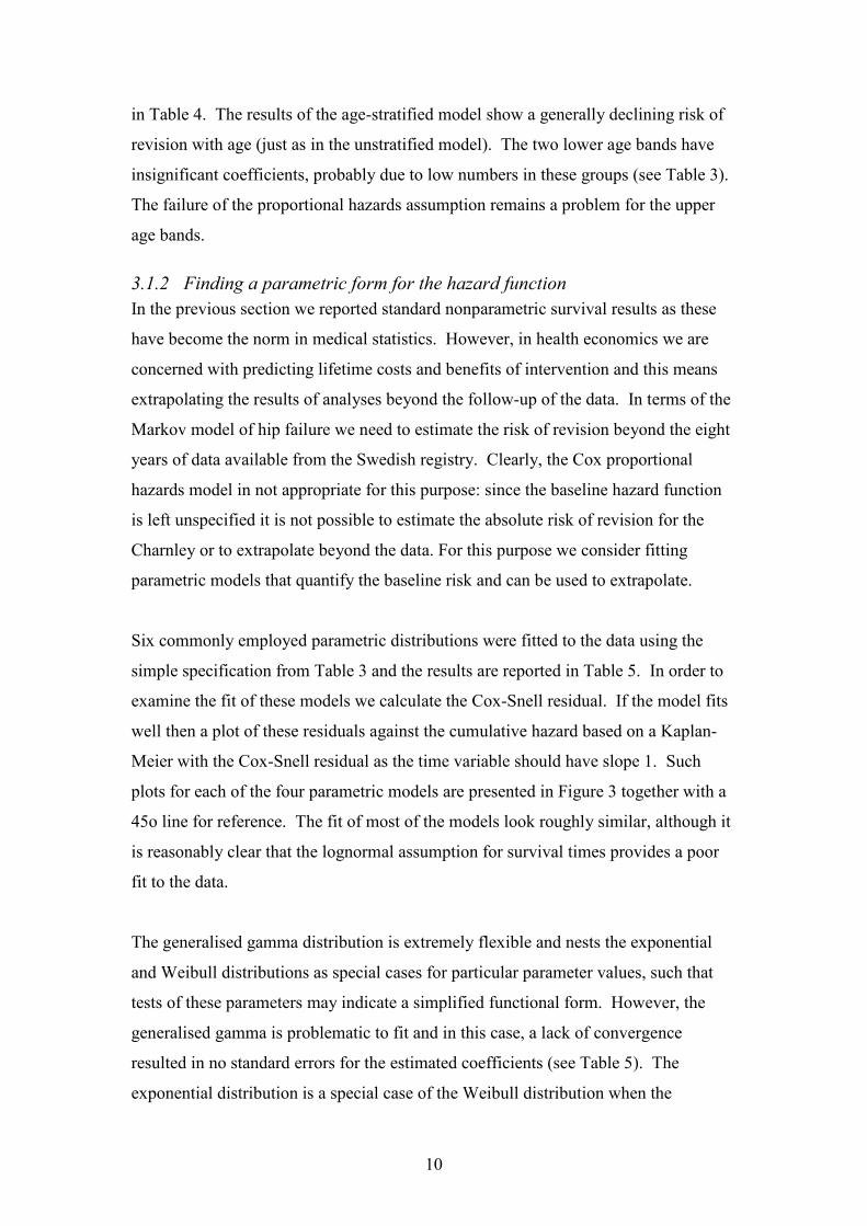
3.1.2 Finding a parametric form for the hazard function In the previous section we reported standard nonparametric survival results as these have become the norm in medical statistics. However, in health economics we are concerned with predicting lifetime costs and benefits of intervention and this means extrapolating the results of analyses beyond the follow-up of the data. In terms of the Markov model of hip failure we need to estimate the risk of revision beyond the eight years of data available from the Swedish registry. Clearly, the Cox proportional hazards model in not appropriate for this purpose: since the baseline hazard function is left unspecified it is not possible to estimate the absolute risk of revision for the Charnley or to extrapolate beyond the data. For this purpose we consider fitting parametric models that quantify the baseline risk and can be used to extrapolate. Six commonly employed parametric distributions were fitted to the data using the simple specification from Table 3 and the results are reported in Table 5. In order to examine the fit of these models we calculate the Cox-Snell residual. If the model fits well then a plot of these residuals against the cumulative hazard based on a Kaplan-Meier with the Cox-Snell residual as the time variable should have slope 1. Such plots for each of the four parametric models are presented in Figure 3 together with a 45o line for reference. The fit of most of the models look roughly similar, although it is reasonably clear that the lognormal assumption for survival times provides a poor fit to the data. The generalised gamma distribution is extremely flexible and nests the exponential and Weibull distributions as special cases for particular parameter values, such that tests of these parameters may indicate a simplified functional form. However, the generalised gamma is problematic to fit and in this case, a lack of convergence resulted in no standard errors for the estimated coefficients (see Table 5). The exponential distribution is a special case of the Weibull distribution when the

11

ancillary parameter is equal to one – thus from Table 5 it is possible to reject the exponential distribution in favour of the Weibull since the ancillary parameter is clearly below one. Choosing between the remaining non-nested models standard likelihood ratio or Wald tests are not appropriate making the problem of choosing between the models more difficult. A common solution is to use the Additional (Aikake’s) Information Criterion (AIC), which proceeds by penalising the log-likelihood in relation to the number of parameters estimated. The AIC is defined as

( ) ( )2 log-likelihood 2 1AIC c p= − + + +

where c represents the number of covariates estimated and p is the number of ancillary parameters employed in the model. The AIC for each model is given in the final row of Table 5 with lower values indicating the preferred model. It turns out that the Gamma distribution has the lowest AIC, but in light of its failure to converge this seems not to be a sensible choice. Of the remaining distributions, the Weibull has the lowest AIC. However, the general observation from the residual plots that there is little to choose between the models is also true of the analysis based on the AIC.

3.1.3 Reasons for failure and ‘bathtub’ curves From the analysis above, the Weibull model was chosen as the most appropriate from for the survival analysis, based on the fit to the data. The Weibull distribution has the following probability density function:

{ }1( ) expf t t tγ γλγ λ−= −

that is characterised by two parameters λ and γ .

The hazard function is: 1( )h t tγλγ −= .

Note that it should be clear from these expressions that in the case of 1γ = , the Weibull expressions above reduce to those of the exponential distribution. The purpose of fitting a parametric model to the data was to allow extrapolation. Figure 3

12

shows the hazard function from the Weibull distribution for a female aged 60 years without an initial diagnosis of fracture who receives the Charnley prosthesis. It is clear from this figure that the estimated hazard function is monotonically decreasing over time with the consequence that extrapolation of this model results in lower and lower hazard rates in future time periods. In fact the monotonically decreasing nature of the hazard function arises from the estimate of the γ parameter as less than one. We might question how realistic the assumption of a decreasing hazard function is – we might expect, for example, that hip prostheses may begin to fail as they reach the end of their useful life. A well known model in the engineering literature is that the lifetimes of components have U-shaped or ‘bathtub’ failure curves, where initially failure rates may be high reflecting faulty or incorrectly fitted components, the rate may then stabilise before rising again as components wear out in use. This seems to be a reasonable model for hip failure and, in consultation with clinical experts, we explored the reasons for revision – these revision reasons are summarised in Table 6. The most frequently recorded reason for revision (59% of all revisions) was deemed to be a long-term revision reason, another three reasons (36% of all reasons) were deemed to be early revision reasons. On the basis of this classification two separate Weibull functions were estimated, one for 338 (59%) of revisions that were considered long term and one for the remaining 236 (41%) of revisions that we label as early revisions. The results of these two separate Weibull regressions are reported in Table 7 and show the expected result that short term failure has a monotonically decreasing hazard function ( 0.5γ ≈ ) while for long term failures the Weibull hazard is increasing ( 1.5γ ≈ ). The combined hazard function, obtained by adding the separate hazard functions for early and late failures, is shown in Figure 5 for a 60-year-old female without an initial diagnosis of fracture receiving the Charnley prosthesis (c.f. Figure 3). This failure curve exhibits the properties that we might consider reasonable a priori – the ‘bathtub’ shape. This is crucial for the modelling since it is the late failure curve that has most effect on the extrapolated failure rates. Notice from Table 7 the effect of separate estimation of failure rates on the significance of the coefficients. It is clear from the early failure model that only an initial fracture diagnosis appears to be a significant predictor of early failure. By

13

contrast, age, sex and prosthesis type are highly significant predictors of late prosthesis failure. Recall that the purpose of this analysis of prosthesis failure rates from the Swedish Registry data is to estimate the transition probability for prosthetic failure in the Markov model – other important parameters to be included are the quality of life values for the different model states and the background mortality rates that represent a competing risk for prosthesis failure. Both the quality of life parameters and mortality rates can be broken down by age and sex. However, no information is available for the effect on quality of life or mortality by an initial diagnosis of fracture. In light of this and in light of the fact that fracture is only predictive of early failure, which has little influence on long term failure rates) we chose to omit the fracture variable from the survival model of prosthesis failure. The model for early and late failure without the fracture covariate are presented in Table 8. We undertook the separate estimation of early and late revisions because we believe the failure curve to be bathtub shaped. However, since the treatment effect of the Spectron is higher in the long-term model and this has most influence on the extrapolated failure rates it might be argued that this approach inflates the treatment effect. Therefore, we also considered a very simple model of a constant hazard rate that was extrapolated. This exponential model is also presented in Table 8. The final parameter estimates required to allow the appropriate propagation of parameter uncertainty through the model are the correlations between the coefficient estimates, obtained from the variance-covariance matrices of the estimated models. The correlation coefficients between each of the coefficient parameters of the three models reported in Table 8 are presented in Table 9.

3.2 Quality of life for hip patients: evidence from the Nuffield Orthopaedic Centre

As part of a wider research agenda,10 patients undergoing total hip replacement at the Nuffield Orthopaedic Centre (NOC), Oxford, United Kingdom, completed an EQ-5D questionnaire at 2-weeks prior to and 12 months after their operation. Overall, age, sex and information on whether the operation was a primary or revision procedure

14

were available for 1,494 patients who fully completed the EQ-5D questionnaire either pre-operation (1,148 patients) or at 12 months post-operation (1,035 patients). In this section we describe the development of regression models that provide an estimate of the quality of life of patients experiencing hip replacement by age and sex of the patient, which can then be employed to provide utility estimates for the states of the Markov model. Only 689 patients (46%) completed a questionnaire both before and at 12 months after the operation. We therefore model the before and after quality of life values using the full set of available data in each case, but adjust for repeated measurement by correlating the resulting models using the observed correlation coefficient for the 689 patients with complete data. Quality of life data are constrained on the interval ( ),1−∞ , although the use of the EQ-5D tariffs in this study to obtain the utility estimates effectively bounds the lower end of the distribution to be equal to the tariff of the worst EQ-5D health state, where a patient has severe problems associated with each dimension of the scale (a tariff value of –0.6). We might consider the non-linear transformation ( ) ( )ln 1z g y y= = − ,where y is the EQ-5D tariff value, in order to apply our modelling to an unconstrained scale. The back-transformation ( ) ( )1 expy h z z= = − can then be used to transform back to the original scale. However, this transformation creates a problem for patients scoring a utility of one (state 11111 of the EQ-5D) since the log of zero is undefined. We return to this problem in the description of the modelling below. The distribution of the quality of life data from the NOC are presented in Figure 6 for the pre- and post-THR procedure and on the raw and transformed scales. The bounding of the data does not seem to be a big problem for scores taken before the THR procedure, which seems reasonable a priori since it is known that the need for hip-replacement is associated with much morbidity. However, one year after the procedure, many patients (over one quarter in this data set) mapped into the best health state in the EQ-5D index and were, therefore, assigned a utility score of one. Due to the problem of the log of zero being undefined the distribution for the transformed post-THR procedure data is shown only for patients recording a utility

15

score less than one. Transformation of the data seems to have considerable effect on the post-THR distribution, but little effect on the pre-THR distribution. Regression models were fitted to the utility data presented in Figure 6 using age, sex and whether the procedure represented a revision operation as explanatory variables and the results are presented in Table 10. Models were fitted on the transformed and untransformed scales and the residual versus fitted value plots for each model of Table 10, are presented in the corresponding panel of Figure 7. For post-THR scores on the transformed scale we employed a Tobit model which treats the utility scores of one that could not be transformed as censored values. This has the effect of distributing the ‘spike’ of the density for individuals scoring an untransformed utility of one, between 0.88 (the highest utility associated with a non 11111 EQ-5D state) and one, after retransformation. Due to the censoring issue, it is not possible to construct a convention residual versus fitted plot – therefore Figure 7(d) shows a plot for a straightforward OLS model on available data on the transformed scale in order to examine the importance of heteroscedasticity. The models on the raw scale exhibit evidence of heteroscedasticity, particularly post-THR, which is to be expected given the bounding of the scale. Models on the transformed scale show less evidence of pattern in the residual versus fitted plots, although there is still some evidence of remaining heteroscedasticity in the post-THR model. Therefore, the chosen models were those on the transformed scale, despite the slightly reduced explanatory power of the post-THR model. To mitigate against any remaining effects of heteroscedasticity, robust standard errors were estimated using the White-corrected variance estimates (Stata Corporation, 2001). The correlation matrix for the regression coefficients of the transformed regression models are presented in Table 11. What is clear from the analysis of the regression results, both on the raw utility and the transformed utility scales is that age, sex and whether the procedure is a revision operation are all important predictors of the health related quality of life experience of patients. While the overall explanatory power of the models is low, the significance of the individual coefficients on the explanatory variables is high.

16

3.3 Other model parameters While the two patient level data sources outlined above provide parameter estimates for the key revision risk and quality of life parameters for the model, there remained a number of remaining parameters that were required for the model. These parameters were obtained from secondary published sources.

3.3.1 Mortality rates In our original model9 we assumed that patients experiencing hip replacement surgery had a survival experience equivalent to those observed in the general population. That is, we assumed that the need for hip replacement only affected patient’s quality of life, not length of life. However, a recent study has directly compared the risk of death following both primary and revision hip replacement procedures to the risk of death observed in the general population.11 Based on over 9,000 primary procedures, the estimated relative risk of death was 1.01 (95% CI: 0.94-1.04) in men and 1.06 (1.03-1.09) in women. For revision procedures (n=1331) the estimated relative risks were 1.07 (0.99-1.15) for men and 1.09 (1.01-1.18) for women. After careful consideration and in consultation with clinical colleagues we decided not to include these increased risks of mortality for two reasons: firstly, the estimates are only statistically significant for women; secondly, there is a danger of double counting if these elevated mortality risks are combined with the operative mortality rates described below. Furthermore, other studies have only found increased mortality rates in the period immediately after operation.12

The other mortality parameter relates to operative mortality rates as part of the procedure and the general risk of undergoing anaesthesia. These proved difficult to obtain from the literature. In the same paper estimating increased mortality risks for patients having undergone a hip replacement procedure, Sodermann and colleagues present a graph of mortality rates against time.11 We took the zero time point on this graph as an estimate of operative mortality (approximately 2.0 % from the graph).

3.3.2 Re-revision risks The Swedish registry data gives a robust method to estimate the risk of revision following primary THR directly. However, there is also a chance that these revisions

17

will have to be re-revised. This information was not available from the data we received from the Swedish registry. Instead we used data from a study of the survival of 109 revision procedures where re-revision was the defined failure endpoint.13 They estimated that at 10 years following revision, 85.4% of the prosthesis had not been revised. We translated this into a constant risk of failure of 1.6% per year. A constant failure risk was considered an appropriate simplifying assumption given the relatively low risk for the initial revision.

3.3.3 Cost of total hip replacement procedures In our original model9 we employed a bottom-up costing procedure based on the clinical experience of surgeons at the Nuffield Orthopaedic Centre, Oxford, in order to come up with a cost estimate of each procedure based on the type of prosthesis (and associated consumables) employed, the time in theatre and the staff present during the procedure. This time we adopted a simpler approach that we believe is more generalisable. Costs of the prostheses themselves were obtained from the published list prices available from the manufacturers: £505 for the Charnley and £715 for the Spectron (579 and £788 respectively, including cement). We assumed that there would be no difference in the procedure costs for the primary THR and that as a consequence it was unnecessary to estimate the cost of a primary THR procedure (since these net out from each arm of the model). For revision procedures, we employed figures produced as part of the NHS reference costing exercise.14 Procedures are grouped into HRGs and mean costs and interquartile ranges are quoted for each group. Primary THR procedures are listed with a mean cost of £3,889 although revision THR procedures do not have an individual entry. Instead revision hip and knee procedures are grouped together: a standard hip/knee revision is listed as £5,294 (interquartile range: £4,034 - £6,040) and a complex hip/knee revision is listed as £6,321 (£2,190). The relative proportions of hip to knee revisions are not known, although a primary knee replacement procedure is listed as £4,390. To adjust the basic figure of £5,294 would require a reduction to allow for the more expensive knee replacement procedure and an increase to allow for some more complex procedures. We therefore take the net effect

18

to be approximately zero and use £5,294 as our estimate of the cost of a revision THR procedure.

3.3.4 Discounting Following UK government guidelines,15 we employ differential discounting - 6% for costs and 1.5% for health outcomes.

4 Parameter distributions for the probabilistic cost-effectiveness analysis

In order to propagate uncertainty through the model, distributions were assigned to all model parameters that are estimated with uncertainty. Distributions are chosen to reflect sampling uncertainty associated with the parameter estimation and this process together with the parametric assumptions employed are outlined below.

4.1 Revision risks The Wiebull distribution is presented in section 3.1.3 above as a function of a scale parameter and an ancillary shape parameter γ . The parameter coefficients from the reduced forms of the Weibull models presented in Table 8 estimate the shape parameter directly and the scale parameter as a linear function of covariates, both on the natural log scale. That is the estimated hazard function is, ( ) ( ) 1

0 1 2 3exp age male spectronh t tγβ β β β γ −= + + + where the β ’s represent estimated coefficients. It should be clear from the above expression that it is the exponential of the coefficients given in Table 8 that give the hazard ratios in the Weibull model. In order to estimate random variates from the estimated models the raw coefficients from Table 8 were assumed to follow a multivariate normal distribution with a correlation structure given by the coefficients from the correlation matrix of Table 9. Cholesky decomposition of the covariance matrix was performed and the correlated random variates, y, obtained from y Tz µ= + , where T is the Cholesky decomposition

19

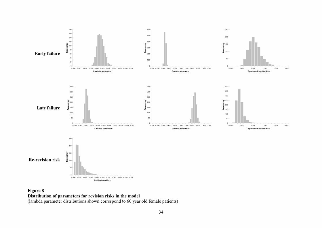
matrix, z is a vector of independent standard normal random variates and µ is the vector of estimated coefficients. The first two rows of Figure 8 show the parameter distributions for the early and late revision equations respectively. The lambda parameter relates to the baseline shape of the Charnley hazard function for a 60 year old female patient. The relative risk of revision with a Spectron prosthesis is shown as a separate distribution. The transition probability for re-revision was estimated as a constant hazard of 1.6% per year from a small study by Hultmark and colleagues.13 Unfortunately, it was not possible from the reported results to accurately estimate a variance for this parameter. Instead, we simply assumed a lognormal distribution (since the hazard must be positive) and a coefficient of variation for the parameter (the ratio of the standard error to the mean) of 0.2. The resulting distribution of the hazard is shown in the final row of Figure 8.

4.2 Utility scores The calculation of utility scores was outlined in Section 3.2 above where it was chosen to estimate utility scores on the transformed scale due to concerns of heteroscedasticity and bounding of the utility scale. The estimated model was 0 1 2 3age male revisioni i i i iz β β β β ε= + + + +

where iz is the transformed utility score, the 'sβ are the estimated coefficients and iεis a random error term. Random variates were obtained from a multivariate normal distribution for the coefficients presented in Table 10(c)&(d) with the correlation matrices presented in Table 11 using the Cholesky decomposition method outlined in Section 4.1 above. In addition, Cholesky decomposition was also employed to correlate the random variables for the before and after THR procedure regressions using the estimated correlation coefficient of 0.26 obtained from patients who completed both the before and after questionnaires. Once random variates were obtained on the transformed scale, these were back-transformed to the original scale. The distribution for the utility estimates (for women aged 60 years) is shown in Figure 9 for each of the states of the model.

20

4.3 Mortality risks Three types of mortality parameters are employed in the model. The first are the background age and sex specific mortality rates obtained from standard life-tables. The second are relative mortality risks for patients undergoing THR procedures compared to the overall population. Finally, there are operative mortality rates related to the procedure itself. Published life-tables are based on large numbers of registered deaths and therefore represent a precise estimate of age and sex specific mortality rates. Nevertheless to represent uncertainty in the estimation of these rates we took the following approach. Yearly rates were available for the last seven years, we therefore estimated the sample variance across the last seven years and used this as an estimate of variance of the estimated rate taken from the most recently available rate (1999). In the presence of trend this will be an overestimate of true variance; however, the trend over the last seven years is expected to be low and therefore the method should be approximately correct. Mortality rates were estimated for all age groups, however, only mortality rates for men and women aged 60 years is presented in the first row of Figure 10. Sodermman and colleagues estimated relative risk of mortality among patients having experienced either a primary or revision THR procedure relative to the general population by gender.11 The authors presented 95% confidence intervals and so the following method to fit distributions were applied. Assuming a lognormal distribution the natural logarithm of the point estimate and confidence limits were taken and the interval range on the log scale calculated. This range was divided by 2 1.96× in order to estimate the standard error on the log scale. A normal random variate on the log scale was generated using the point estimate and standard error estimated as described above – this random variate was then exponentiated to give a log-normally distributed relative risk. The relative risk distribution following primary and revision procedures are shown in Figure 10 by gender. Operative mortality rates were estimated by interpolation from a figure in Sodermann et al11 and it was therefore not possible to obtain a reliable estimate of variance of the parameter. We therefore assumed that the parameter followed a beta distribution with

21

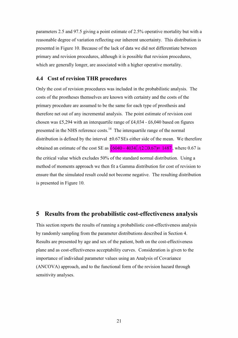
parameters 2.5 and 97.5 giving a point estimate of 2.5% operative mortality but with a reasonable degree of variation reflecting our inherent uncertainty. This distribution is presented in Figure 10. Because of the lack of data we did not differentiate between primary and revision procedures, although it is possible that revision procedures, which are generally longer, are associated with a higher operative mortality.

4.4 Cost of revision THR procedures Only the cost of revision procedures was included in the probabilistic analysis. The costs of the prostheses themselves are known with certainty and the costs of the primary procedure are assumed to be the same for each type of prosthesis and therefore net out of any incremental analysis. The point estimate of revision cost chosen was £5,294 with an interquartile range of £4,034 - £6,040 based on figures presented in the NHS reference costs.14 The interquartile range of the normal distribution is defined by the interval 0.67± SEs either side of the mean. We therefore obtained an estimate of the cost SE as ( )6040 4034 /(2 0.67) 1487− × = , where 0.67 is the critical value which excludes 50% of the standard normal distribution. Using a method of moments approach we then fit a Gamma distribution for cost of revision to ensure that the simulated result could not become negative. The resulting distribution is presented in Figure 10.

5 Results from the probabilistic cost-effectiveness analysis This section reports the results of running a probabilistic cost-effectiveness analysis by randomly sampling from the parameter distributions described in Section 4. Results are presented by age and sex of the patient, both on the cost-effectiveness plane and as cost-effectiveness acceptability curves. Consideration is given to the importance of individual parameter values using an Analysis of Covariance (ANCOVA) approach, and to the functional form of the revision hazard through sensitivity analyses.

22

5.1 Age and sex adjusted results Before considering the probabilistic results, the point estimates of incremental cost and QALYs by age and sex are presented on the cost-effectiveness plane in Figure 11. Results are shown separately for males and females and for age at primary THR procedure of 40, 50, 60, 70, 80 and 90 years. The dotted lines in the figure indicate the estimate of a continuous age function and should not be interpreted as representing incremental cost-effectiveness ratios. Incremental ratios would be obtained for any age by the slope of the line joining that point to the origin of the figure. It is clear that for younger ages for both men and women, the Spectron dominates the Charley prosthesis, being both cost saving and associated with increased QALYs. The difference between the sexes diminishes as patients get older – this makes sense since both age curves are tending toward the same point – the greater a patient’s age the more important the natural death rate as a competing risk with prosthesis failure. In the limit, where a patient will almost certainly die before prosthesis failure, the Spectron will be £209 more expensive than the Charnley (the simple difference in the prosthesis costs) and will have no QALY benefits. Of course, the results presented in Figure 11 are subject to uncertainty and this is precisely what the probabilistic cost-effectiveness analysis is designed to capture. For example, in Figure 12(a) the results of 1,000 random evaluations of the model for women aged 60 years are presented on the cost-effectiveness plane and in Figure 12(b) these simulation results are summarised as a cost-effectiveness acceptability curve. The results show that for 60-year-old women, the Spectron is a highly cost-effective use of resources, even when all the appropriate parameter uncertainties are taken into account. The base case age and sex adjusted results are presented in Table 12 and as a series of cost-effectiveness acceptability curves in Figure 13. The results show that for all but the eldest patients, the cost-effectiveness of the Spectron is clear, even when uncertainty is taken into account. Overall, the cost-effectiveness for men is greater than that for women, which is largely driven by the greater revision risk for males apparent from the hazard models of Section 3.1.

23

5.2 Sensitivity analyses The probabilistic cost-effectiveness analysis reported above is effectively a probabilistic sensitivity analysis that captures the joint uncertainty in all parameters simultaneously. However, two aspects of the analysis deserve further consideration. Firstly, consideration is given to the individual contribution of each parameter in the model. Secondly, we consider the use of an alternative functional form for the revision hazard function.

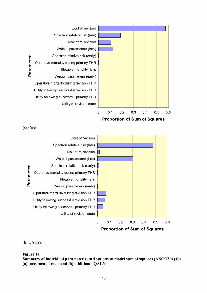
5.2.1 Parameter importance Although the analysis reported in Section 5.1 above gives a useful representation of the overall uncertainty in the model, it is still interesting to note the contribution made by individual model parameters. To do this we recorded the values of the input parameters in addition to the addition costs and QALY outputs from the model and we used and Analysis of Covariance (ANCOVA) approach (equivalent to linear regression) to explore the proportion of the total model sums of squares that was explained by each individual model input parameter. This approach assumes a linear relationship between the input parameters (explanatory variables) and the output parameters (dependent variables) when in fact the overall model is non-linear. However, since the ANCOVA model explains over 95% of the variation for each of the cost and QALY output variables, it is clear that the linear model is a good approximation. A summary of the ANCOVA results applied separately to (a) incremental costs and (b) incremental QALYs is presented in Figure 14. This analysis suggests that it is the relative risk of late failure for the Spectron prosthesis, the cost of the revision procedure and the baseline risk of late revision for the Charnley prosthesis that are most important in explaining variation in the overall results. It is on the better estimation of these parameters that future research should focus if better estimates of cost-effectiveness are required.

24

5.2.2 Risk functional form Given the way in which the hazard functions for revision were extrapolated in the form of a ‘bath-tub’ failure curve (see Section 3.1.3), it is not surprising that it is the late failure estimates of absolute revision risk for the Charnley and relative revision risk for the Spectron that were identified as key parameters in the analysis of the previous section. However, this may raise the concern that the results are merely dependent on the particular approach to modelling the hazard function. For this reason we repeat the main analysis employing a different form for the hazard function: instead of estimating separate early and late hazards, we simply estimate a constant (exponential) hazard function which we then extrapolate beyond the follow-up of the registry data. The results of this reanalysis based on the exponential distribution of survival times (constant hazard of revision) is presented in Table 13 and in Figure 15. Overall, the results are slightly less favourable for the Spectron as the extrapolated hazard is somewhat lower than that under the assumption of the increasing hazard of late failures in the base case analysis. However, from a policy perspective, the Spectron still looks to be very good value for money for most age groups.

6 Summary This report has provided detailed documentation on the modelling of the cost-effectiveness of the Spectron prosthesis relative to the Charnley. The cost-effectiveness model presented here indicates that, based on mean costs and QALYs and compared to the Charnley, the Spectron is cost saving in younger patients, and generates incremental cost-effectiveness ratios of between £1,000 and £16,000 in older patient groups. Allowing for uncertainty in parameter estimates, the probability of the Spectron being more cost-effective than the Charnley ranges from 70% to 100%.

25

References

1. Fitzpatrick, R, Shortall, E, Sculpher, M et al. Primary total hip replacement surgery: a systematic review of outcomes and modelling of cost-effectiveness associated with different prostheses . Health Technology Assessment 1998;2 (20).

2. Chang, RW, Pellissier, JM, and Hazen, GB. A cost-effectiveness analysis of total hip arthroplasty for osteoarthritis of the hip. Journal of the American Medical Association 1996;275:858-865.

3. Williams M, Frankel S, Nanchanal K, Coast J, Donovan J. Epidemiologically Based Needs Assessment. Total Hip Replacement. DHA Project: Research programme commisioned by the NHS Management Executive. London: Crown Publisher, 1992.

4. Murray, DW, Carr, AJ, and Bulstrode, CJ. Which primary total hip replacement? Journal of Bone and Joint Surgery 1995;77B:520-527.

5. National Institute for Clinical Excellence. Guidance on the Selection of Prostheses for Primary Total Hip Replacement (www.nice.org.uk). London: National Institute for Clinical Excellence, 2000.

6. Herberts, P and Malchau, H. Long-term registration has improved the quality of hip replacement: a review of the Swedish THR Register comparing 160,000 cases. Acta Orthopaedica Scandinavica 2000;71:111-21.

7. Daellenbach, HG, Gillespie, WJ, Crosbie, P et al. Economic appraisal of new technology in the absence of survival data - the case of total hip replacement. Social Science and Medicine 1990;31:1287-1293.

8. Gillespie, WJ, Pekarsky, B, and O'Connell, DL. Evaluation of new technologies for total hip replacement: economic modelling and clinical trials. Journal of Bone and Joint Surgery 1995;77B:528-533.

9. Briggs, A, Sculpher, M, Britton, A et al. The costs and benefits of primary total hip replacement. How likely are new prostheses to be cost-effective? International Journal of Technology Assessment in Health Care 1998;14:4:743-761.

10. Dawson, J, Fitzpatrick, R, Frost, S et al. Evidence for the validity of a patient-based instrument for assessment of outcome after revision hip replacement. JBone Joint Surg 2001;83-B:1125-9.

11. Soderman, P, Malchau, H, Herberts, P et al. Are the findings in the Swedish National Total Hip Arthroplasty Register valid? A comparison between the Swedish National Total Hip Arthroplasty Register, the National Discharge Register, and the National Death Register. The Journal of Arthroplasty 2000;15:884-889.

12. Seagroatt, V, Tan, HS, Goldacre, M et al. Elective total hip replacement; incidence, emergency readmission rate, and postoperative mortality. British Medical Journal 1991;303:1431-1435.

13. Hultmark, P, Karrholm, J, Stromberg, C et al. Cemented first time revisions of

26

femoral component. Prospective 7 to 13 years' follow-up using second generation and third generation technique. The Journal of Arthroplasty 2000;15:551-561.

14. NHS Executive. The New NHS - 2000 Reference Cost (http://www.doh.gov.uk/nhsexec/refcosts.htm#down). London: NHS Executive, 2001.

15. Department of Health. Policy Appraisal and Health. London: Department of Health, 1995.

27

Primary THR

Revision THR

Successful Primary Death

Successful Revision

Figure 1 State transition diagram of the Markov model for hip replacement

28

Kapla

n-Meie

rS(t)

analysis time0 2 4 6 8

.9

.95

1Spectron

Charnley

Figure 2 Kaplan-Meier estimate of the survivor function by type of prosthesis

29

Exponential-ln

(Kap

lan-M

eier)

Cox-Snell residual0 .1 .2 .3

0

.1

.2

.3Weibull

-ln(K

aplan

-Meie

r)


0

.1

.2

.3

Log-Normal

-ln(K

aplan

-Meie

r)


0

.1

.2

.3Log-logistic

-ln(K

aplan

-Meie

r)


0

.1

.2

.3

Gompertz

-ln(K

aplan

-Meie

r)


0

.1

.2

.3Generalised Gamma

-ln(K

aplan

-Meie

r)


0

.1

.2

.3

Figure 3 Residual plots for six possible parametric survival models

30

Maximum follow-up

00.002

0.0040.0060.008

0.01

0.0120.0140.0160.018

0.02

0 5 10 15 20 25 30analysis time

Haza

rdfu

nctio

n

Figure 4 Weibull hazard function for a female aged 60 without initial diagnosis of fracture who receives a Charnley implant The solid line indicates the fit to the data and the dotted line indicates the extrapolated hazard beyond the follow-up period.

31

0.00%

0.20%

0.40%

0.60%

0.80%

1.00%

1.20%

1.40%

0 5 10 15 20Years

Tran

sition

prob

abilit

yMaximumfollow-up

Early failure

Combined failure

Late failure

Figure 5 Modelling early and late failure probabilities separately in order to obtain a ‘bathtub’ failure curve

32

(a)

Frac

tion

Utility score pre-THR-.6 0 .5 1

0

.1

.2

.3

(b)

Frac

tion

Utility score 12 months post-THR-.6 0 .5 1

0

.1

.2

.3

(c)

Frac

tion

Transformed utility score pre-TH-2 -1 0 1

0

.1

.2

.3

(d)Fr

actio

nTransformed utility score 12 mon

-2 -1 0 10

.1

.2

.3

Figure 6Quality of life scores for (a)&(c) Pre-THR procedure and (b)&(d) 12-months post THR on the (a)&(b) Untransformed and (c)&(d)Transformed utility scales(Note that the distribution in (d) omits those patients who score a full health utility of one on the untransformed scale)

33

(a)

Resid

uals

Fitted values.251663 .434291

-.903899

.726495

(b)

Resid

uals

Fitted values.422513 .823931

-1.34034

.577487

(c)

Resid

uals

Fitted values-.699347 -.39916

-1.66884

.998363

(d)Re

sidua

lsFitted values

-1.30014 -.781158-1.24409

1.57046

Figure 7Residual versus fitted plots for the best fitting models from Table 10 for (a)&(c) Pre-THR procedure and (b)&(d) 12-months post THRon the (a)&(b) Untransformed and (c)&(d) Transformed utility scales(note that (d) plots the residuals from a model on uncensored utility only, not the Tobit model from Table 10)

34

Early failure

0

20

40

60

80

100

120

140

160

180

0.000 0.001 0.002 0.003 0.004 0.005 0.006 0.007 0.008 0.009 0.010Lambda parameter

Freq

uenc

y

0

100

200

300

400

500

600

0.000 0.200 0.400 0.600 0.800 1.000 1.200 1.400 1.600 1.800 2.000Gamma parameter

Freq

uenc

y

0

50

100

150

200

250

0.000 0.400 0.800 1.200 1.600 2.000Spectron Relative Risk

Freq

uenc

y

Late failure

0

50

100

150

200

250

300

350

0.000 0.001 0.002 0.003 0.004 0.005 0.006 0.007 0.008 0.009 0.010Lambda parameter

Freq

uenc

y

0

50

100

150

200

250

300

350

0.000 0.200 0.400 0.600 0.800 1.000 1.200 1.400 1.600 1.800 2.000Gamma parameter

Freq

uenc

y

0

50

100

150

200

250

300

350

400

0.000 0.400 0.800 1.200 1.600 2.000Spectron Relative Risk

Freq

uenc

y

Re-revision risk

0

50

100

150

200

250

0.000 0.020 0.040 0.060 0.080 0.100 0.120 0.140 0.160 0.180 0.200Re-Revision Risk

Freq

uenc

y

Figure 8Distribution of parameters for revision risks in the model(lambda parameter distributions shown correspond to 60 year old female patients)

35

Utility scores

0

50

100

150

200

250

300

350

400

450

0.40 0.50 0.60 0.70 0.80 0.90 1.00Successful Primary THR

Freq

uenc

y

0

50

100

150

200

250

0.40 0.50 0.60 0.70 0.80 0.90 1.00Successful Revision THR

Freq

uenc

y

0

50

100

150

200

250

300

0.40 0.50 0.60 0.70 0.80 0.90 1.00Revision of THR

Freq

uenc

y

Figure 9Distribution of utility scores for each state in the model (for women aged 60 years)

36

Backgroundmortality rates

0

50

100

150

200

250

5 6 7 8 9 10 11 12 13 14 15Deaths per 1,000 per year (females)

Freq

uenc

y0

20

40

60

80

100

120

140

5 6 7 8 9 10 11 12 13 14 15Deaths per 1,000 per year (males)

Freq

uenc

y

Operative mortality rate

020

4060

80

100120

140

160180

200

0 0.02 0.04 0.06 0.08 0.1Operative mortality rate

Freq

uenc

y

Cost of revision THR procedure

0

20

40

60

80

100

120

140

160

£0 £2,000 £4,000 £6,000 £8,000 £10,000 £12,000Cost of revision THR

Freq

uenc

y

Figure 10 Mortality and cost parameter distributions

37

9080

70

60

50

40

8090

70

60

50

40

-£1,200

-£1,000

-£800

-£600

-£400

-£200

£-

£200

£400

-0.2 0.0 0.2 0.4 0.6 0.8 1.0

Additional QALYs

Incre

ment

alco

stMalesFemales

Figure 11 Point estimate results on the cost-effectiveness plane by age and sex

38

-£800

-£700

-£600

-£500

-£400

-£300

-£200

-£100

£-

£100

£200

0.00 0.05 0.10 0.15 0.20 0.25 0.30 0.35QALYs gained

Addit

ional

Cost

(a)

0.00

0.10

0.20

0.30

0.40

0.50

0.60

0.70

0.80

0.90

1.00

£- £5,000 £10,000 £15,000 £20,000Value of ceiling ratio

Prob

abilit

ycos

t-effe

ctive

(b) Figure 12 Results of probabilistic cost-effectiveness analysis for the Spectron prosthesis in women aged 60 years presented (a) on the cost-effectiveness plane and (b) as an acceptability curve

39

00.10.20.30.40.50.60.70.80.9

1


Prob

abilit

ycos

t-effe

ctive

Age 40Age 50Age 60Age 70Age 80Age 90

(a) Males

00.10.20.30.40.50.60.70.80.9

1


Prob

abilit

ycos

t-effe

ctive


(b) Females Figure 13 Acceptability curves for the cost-effectiveness of the Spectron prosthesis by age for (a) males and (b) females

40

0 0.1 0.2 0.3 0.4 0.5 0.6

Utility of revision stateUtility following successful primary THRUtility following successful revision THROperative mortality during revision THR

Weibull parameters (early)lifetable mortality risks

Operative mortality during primary THRSpectron relative risk (early)

Weibull parameters (late)Risk of re-revision

Spectron relative risk (late)Cost of revision

Para

meter

Proportion of Sum of Squares

(a) Costs

0 0.1 0.2 0.3 0.4 0.5 0.6

Utility of revision stateUtility following successful primary THRUtility following successful revision THROperative mortality during revision THR

Weibull parameters (early)lifetable mortality risks

Operative mortality during primary THRSpectron relative risk (early)

Weibull parameters (late)Risk of re-revision

Spectron relative risk (late)Cost of revision

Para

meter

Proportion of Sum of Squares

(b) QALYs Figure 14 Summary of individual parameter contributions to model sum of squares (ANCOVA) for (a) incremental costs and (b) additional QALYs

41

00.10.20.30.40.50.60.70.80.9

1


Prob

abilit

ycos

t-effe

ctive


(a) Males

00.10.20.30.40.50.60.70.80.9

1


Prob

abilit

ycos

t-effe

ctive


(b) Females Figure 15 Probabilistic cost-effectiveness results by age for (a) Males and (b) Females assuming an exponential survival distribution

42

Table 1 Log-rank test for the equality of the survivor functions Prosthesis Observed Expected

Spectron 22 51.06Charnley 552 522.94

Total 574 574

chi2(1) = 18.18Pr>chi2 = <0.0001

Table 2 Summary statistics for patients in the Swedish Registry receiving either a Charnley or Spectron prosthesis as a primary hip replacement Charnley Spectron

patients 18505 1990mean age (sd) 72 (9.2%) 74 (8.1%)Age distribution (%) <40 years 70 (0.4%) 5 (0.3%) 40-50 years 264 (1.4%) 16 (0.8%) 50-60 years 1418 (7.7%) 60 (3.0%) 60-70 years 4836 (26.1%) 391 (19.7%) 70-80 years 8090 (43.7%) 1014 (51.0%) 80-90 years 3630 (19.6%) 481 (24.2%) >90 years 197 (1.1%) 23 (1.2%)Gender (%) female 12337 (66.7%) 1472 (74.0%) male 6168 (33.3%) 518 (26.0%)Initial diagnosis (%) Osteoarthritis 12970 (70.1%) 1348 (67.7%) Fracture 1692 (9.1%) 319 (16.0%) Other 3843 (20.8%) 323 (16.2%)

43

Table 3 Cox proportional hazards model Explanatory variable Hazard Ratio* SE

spectron 0.435 0.095age** 0.974 0.004male 1.785 0.150fracture 1.718 0.221*All coefficients significant at the p<0.001 level **Age coefficient failed the test of proportional hazards

Table 4 Cox proportional hazard stratified on age Explanatory variable* Hazard Ratio SE P value

spectron 0.433 0.094 <0.001 age <40 0.847 0.602 0.815 age 40-50 1.289 0.370 0.378 age 50-60 1.369 0.199 0.030 age 70-80** 0.790 0.078 0.018 age 80+** 0.521 0.073 <0.001 male 1.772 0.150 <0.001 fracture 1.742 0.225 <0.001 *Comparison group is aged 60-70 **Age coefficients failed the test of proportional hazards

44

Table 5Alternative parametric specifications for the survival analysis

Exponential Weibull Log Normal Log Logistic Gompertz Gamma*coefficient(SE) coefficient(SE) coefficient(SE) coefficient(SE) coefficient (SE) coefficient (SE)

Constant** 5.625(0.477) 3.753(0.385) 3.630(.)spectron 0.436(0.095) 0.427(0.093) 1.055(0.269) 1.040(0.270) 0.431(0.094) 1.042(.)age 0.974(0.004) 0.974(0.004) 0.032(0.006) 0.032(0.005) 0.974(0.004) 0.032(.)male 1.788(0.151) 1.783(0.150) -0.776(0.124) -0.710(0.107) 1.785(0.150) -0.702(.)fracture 1.721(0.221) 1.712(0.220) -0.820(0.188) -0.672(0.162) 1.717(0.221) -0.640(.)ancillary (1) - 0.818(0.031) 3.240(0.113) 1.210(0.046) -0.046(0.022) 0.515(.)ancillary (2) - - - - - 2.395(.)

log L -3196 -3181 -3202 -3183 -3194 -3180AIC 6402 6375 6416 6377 6400 6374*No standard errors available due to lack of convergence**No constants reported for Exponential, Weibull or Gompertz: presented in hazard ratio form – other distributions in accelerated time form.

45

Table 6 Reasons for revision given in the Swedish Registry together with a classification of whether the reasons are related to early or late revisions

Revision Reason Frequency Percentage Classification

1 ??? 2. Primary deep injection 5. Dislocation 6. Technical problem x. Other

338 72 94 21 49

59% 13% 16% 4% 8%

Late Early Early Early

Unknown Total 574 100%

Table 7 Separate Weibull models for early and late prosthesis failures Early failures Late failures

Hazard ratio(SE) P value Hazard ratio(SE) P value

spectron 0.637(0.171) 0.093 0.258(0.099) 0.000 age40 0.992(0.007) 0.255 0.963(0.005) 0.000 male 1.352(0.183) 0.025 2.177(0.238) 0.000 fracture 2.203(0.387) 0.000 1.303(0.251) 0.170 gamma 0.485(0.030) 1.454(0.069)

46

Table 8Reduced Weibull models for early and late failures plus exponential model for overall failure rate

Early failures Late failures ExponentialRaw

coefficient(SE)Hazard

ratio P valueRaw

coefficient(SE)Hazardratio P value

Rawcoefficient(SE)

Hazardratio P value

constant -5.351(0.276) - 0.000 -5.491(0.208) - 0.000 -4.466(0.140) - 0.000spectron -0.242(0.270) 0.785 0.133 -1.344(0.383) 0.261 0.000 -0.805(0.218) 0.447 0.000age40 -0.002(0.008) 0.998 0.599 -0.037(0.005) 0.964 0.000 -0.024(0.004) 0.976 0.000male 0.305(0.149) 1.356 0.056 0.769(0.109) 2.157 0.000 0.557(0.084) 1.745 0.000gamma -0.813(0.069) 0.444 - 0.374(0.047) 1.454 - - - - -

47

Table 9 Correlations between the coefficients in the three models reported in Table 7 spectron age male constant gamma

Early failures (Weibull)spectron 1age -0.064 1male 0.023 0.081 1constant 0.027 -0.983 -0.18 1 gamma 0.012 -0.005 0.00 -0.082 1Late failures (Weibull)spectron 1age -0.056 1male 0.005 0.044 1constant 0.026 -0.931 -0.189 1 gamma 0.015 -0.005 0.011 -0.301 1All failures (Exponential)spectron 1age -0.064 1male 0.011 0.06 1constant 0.034 -0.98 -0.188 1

48

Table 10The ‘best’ fitting models for estimating quality of life scores for (a)&(c) Pre-THR procedure and (b)&(d) 12-months post THR on the(a)&(b) Untransformed and (c)&(d) Transformed utility scales (for residual plots see Figure 7)

pre-THR Coefficient SE P-Value pre-THR Coefficient SE P-Value

constant 0.294 0.024 0.000 constant 0.676 0.031 0.000age 0.000 0.001 0.524 age40 0.006 0.002 0.002age40^2 age40^2 0.000 0.000 0.002male 0.117 0.019 0.000 male 0.072 0.017 0.000revision -0.036 0.022 0.112 revision -0.145 0.019 0.000Adjusted R2=0.03Cook-Weisberg heteroscedasticity test: P=0.05

Adjusted R2=0.08Cook-Weisberg heteroscedasticity test: P<0.0001

(a) (b)

pre-THR Coefficient SE P-Value pre-THR Coefficient SE P-Value

constant -0.456 0.040 0.000 constant -1.658 0.077 0.000age40 -0.001 0.001 0.372 age40 0.001 0.002 0.692male -0.188 0.031 0.000 male -0.226 0.058 0.000revision 0.042 0.038 0.267 revision 0.503 0.058 0.000Adjusted R2=0.03Cook-Weisberg heteroscedasticity test: P=0.58

Adjusted R2=0.03

(c) (d)

49

Table 11 Correlation coeffiecients between the coefficients of the transformed utility models of Table 9 constant age male revision

Pre-THR procedure constant 1 age -0.839 1 male -0.381 0.063 1 revision -0.196 0.010 -0.029 1

12 months post-THR procedure constant 1 age -0.838 1 male -0.351 0.043 1 revision -0.332 0.032 0.033 1

50

Table 12Base case results for the cost-effectiveness of the Spectron versus Charnley prosthesis by age and sex (Weibull hazard function)Patient group Charnley Spectron ICER Probability

Costs QALYs Costs QALYs cost-effective*

Male40 years £ 2,664 20.6 £ 1,624 21.5 Spectron Dominates 1.0050 years £ 2,017 16.6 £ 1,309 17.1 Spectron Dominates 1.0060 years £ 1,421 12.3 £ 1,083 12.5 Spectron Dominates 1.0070 years £ 1,009 8.3 £ 939 8.3 Spectron Dominates 1.0080 years £ 776 5.2 £ 860 5.2 £ 3,768 1.0090 years £ 693 4.0 £ 833 4.0 £ 11,697 0.91

Female40 years £ 1,892 21.7 £ 1,255 22.5 Spectron Dominates 1.0050 years £ 1,430 17.9 £ 1,080 18.3 Spectron Dominates 1.0060 years £ 1,078 13.7 £ 959 13.9 Spectron Dominates 1.0070 years £ 842 9.5 £ 882 9.5 £ 673 1.0080 years £ 700 5.9 £ 834 5.9 £ 7,000 0.9990 years £ 649 4.6 £ 818 4.6 £ 16,839 0.70

51

Table 13Base case results for the cost-effectiveness of the Spectron versus Charnley prosthesis by age and sex (Exponential hazard function)Patient group Charnley Spectron ICER Probability

Costs QALYs Costs QALYs cost-effective*

Male40 years £ 1,931 21.2 £ 1,477 21.6 Spectron Dominates 1.0050 years £ 1,547 16.9 £ 1,262 17.1 Spectron Dominates 1.0060 years £ 1,212 12.4 £ 1,089 12.5 Spectron Dominates 1.0070 years £ 945 8.3 £ 958 8.3 £ 261 1.0080 years £ 778 5.2 £ 880 5.2 £ 5,640 0.9990 years £ 702 4.0 £ 845 4.1 £ 13,155 0.86

Female40 years £ 1,471 22.1 £ 1,223 22.5 Spectron Dominates 1.0050 years £ 1,225 18.1 £ 1,101 18.3 Spectron Dominates 1.0060 years £ 1,006 13.8 £ 990 13.9 Spectron Dominates 1.0070 years £ 827 9.5 £ 904 9.5 £ 1,652 1.0080 years £ 712 5.9 £ 850 5.9 £ 7,829 0.9990 years £ 662 4.6 £ 827 4.6 £ 15,655 0.77* Based on the health service being willing to pay up to £20,000 per additional QALYICER=incremental cost-effectiveness ratio.

Documents

Modelling the cost-effectiveness of primary hip