Embed Size (px)
Citation preview
MODELLING THE AUSTRALIAN EXCHANGE RATE, LONGBOND YIELD AND INFLATIONARY EXPECTATIONS
Alison Tarditi
Research Discussion Paper
9608
November 1996
Economic Analysis Department
Reserve Bank of Australia
This is a revised version of a paper prepared for the Bank for InternationalSettlements Central Bank Econometrics Meeting, 14th-15th December 1995. I amvery grateful to Lynne Cockerell and John Simon for enthusiastic researchassistance. Thanks also to John Romalis for execution of the macroeconomic modelsimulations and to David Gruen, Philip Lowe and Malcolm Edey for draftingcomments. The views expressed are those of the author and are not necessarilythose of the Reserve Bank of Australia.
Abstract
More than two decades have passed since the initial relaxation of domestic interestrate controls in Australia and just over one decade since the float of the Australiandollar. Interest rates and exchange rates now constitute two of the most importantchannels through which macroeconomic policy can affect the broader economy. It iswidely recognized that expectations play a critical role in these mechanisms,affecting both the timing and speed with which interest and exchange rates transmitshocks through to real activity and prices. Over the longer run, the influence of thesetwo asset prices extends to the efficient allocation of capital and resources. Thispaper builds on previous work undertaken at the Reserve Bank and the OECD todevelop single-equation, behavioural models of these two variables. Considerationis paid to the role of inflation expectations in affecting their behaviour. In particular,a model of ex ante real bond yields is estimated using a measure of forward-lookinginflationary expectations which has been constructed by recourse to a Markovswitching technique.
JEL Classification Numbers F31, E43, E44, C32.
Table of Contents
1. Introduction 1
2. The Macroeconomic Model Approach 2
2.1 Exchange Rate Determination 3
2.2 Interest Rate Determination 5
2.3 Response to Shocks 6
2.4 Assessment 9
3. A Behavioural Model of the Australian Real Exchange Rate 11
3.1 What Determines the Australian Real Exchange Rate? 11
3.2 The Empirical Results 18
4. A Behavioural Model of the Australian Long-Term Interest Rate 26
4.1 The Real Bond Yield Fundamentals in Brief 26
4.2 Measuring Inflationary Expectations 30
4.3 Empirical Results for the Long Bond Yield Equation With Forward-Looking Inflationary Expectations 35
5. Conclusion 40
Appendix A: Data Sources 42
Appendix B: The Behavioural Model of the Australian Real Exchange Rate –Integration Tests and Diagnostics 46
Appendix C: The Behavioural Model of Australian Long Bond Yields – IntegrationTests and Diagnostics 51
REFERENCES 56
MODELLING THE AUSTRALIAN EXCHANGE RATE, LONGBOND YIELD AND INFLATIONARY EXPECTATIONS
Alison Tarditi
1. Introduction
More than two decades have passed since the initial relaxation of domestic interestrate controls in Australia and just over one decade since the float of the Australiandollar. Interest rates and exchange rates now constitute two of the most importantchannels through which macroeconomic policy can affect the broader economy. It iswidely recognized that expectations play a critical role in these mechanisms,affecting both the timing and speed with which interest and exchange rates transmitshocks through to real activity and prices. Over the longer run, their influenceextends to the efficient allocation of capital and resources. This paper developsempirical models of each of these variables for Australia.
Section 2 begins with a brief review of the exchange rate and bond rate equations intwo of Australia’s existing macroeconomic models. These large-scale models offerthe convenience of an internally-consistent link between these asset price variablesand the real economy and typically embody forward-looking financial sectorexpectations. Their exchange rate and long bond rate equations reflect orthodoxtheoretical relationships; they are not estimated equations. The textbook-styleimpulse responses obtained from the macroeconomic modelling of exchange rateand bond rate behaviour offer useful baseline profiles. But the distinctive behaviourof these asset prices, observed in the data in practice, is not fully captured by themacroeconomic model approach. Policymakers need to think more critically aboutthe determinants of these variables since they consititute two of the most importantchannels of policy transmission. To this end, the remainder of the paper builds onprevious work undertaken at the Reserve Bank and the OECD to develop single-equation, behavioural models of the Australian real exchange rate and long bondyield, respectively. In particular, some attention is paid to the role that inflationexpectations might play in affecting these two asset prices.
Section 3 builds on the wealth of earlier applied econometric studies of theAustralian real exchange rate. This previous literature identifies roles for the terms
2
of trade, net foreign liabilities and long-term interest differentials in determiningexchange rate movements. The paper adds, to these factors, direct roles formacroeconomic policy and inflation expectations, which are found to improve theperformance of the model.
In contrast, very little work has been undertaken in Australia on modelling thebehaviour of long bond rates. Section 4 draws on work undertaken at the OECD byOrr, Edey and Kennedy (1995). This work identifies a comprehensive list of thefundamental determinants of real long-term yields across a 17 country panel dataset, including Australia. This paper trials these determinants in a time-series modelof the Australian ex ante real long bond rate. This time-series specification suffersseveral inadequacies and raises the question of how best to transform nominal bondyields into real magnitudes. Because inflation expectations are largely unobservable,the paper spends some time exploring one possible methodology for theirmeasurement.
In practice, inflationary expectations can be heavily conditioned on a country’shistorical inflation performance. In Australia, successful inflation reduction policiesin the early 1990s appear to have been accompanied by falls in existing measuredinflationary expectations series. Section 4.2 discusses some inadequacies of theseexisting measures and estimates an alternative, forward-looking inflationaryexpectations series. For this purpose, a Markov switching technique is used. Thismethodology endogenises shifts in the series and produces estimates of theprobabilities associated with remaining in particular (high or low) inflationaryregimes. A model of the long-term bond yield, deflated with this unconventionalforward-looking series, performs quite well. Section 5 concludes.
2. The Macroeconomic Model Approach
This section focuses on two widely quoted macroeconomic models of the Australianeconomy: the Murphy model and the TRYM model.1. These macro models embody
1 The current (1995) version of the Murphy model consists of 538 equations. TRYM was
developed between 1990 and 1993 and consists of 23 estimated equations, 3 financial marketidentities, 2 default response functions for monetary and fiscal policy and about 100 identitieslinking these key variables (Downes 1995).
3
similar philosophies, sharing many common features of design and specification.They have similar theoretical underpinnings, with Keynesian properties in the shortrun (prices are sticky and output is demand-determined) and neoclassical propertiesin the long run. Equations describing the exchange rate and the long-term bond yieldare elements of the financial sectors of these models and reflect orthodox theoreticalconsiderations; they are not estimated behavioural equations. This section brieflydiscusses these two financial sector equations and their implied responses to shocks.
The process of expectations formation is central to the performance of themacro-model equations. Financial sector expectations are typically assumed to bemodel-consistent. In particular, inflation expectations are constructed from somecombination of the current inflation rate and the equilibrium inflation rate which isderived from the steady-state version of the model. The equilibrium inflation rate issecured in the long run by assuming that the authorities have an exogenously-determined target for some nominal variable. In TRYM, the authorities target themoney growth path; in recent versions of the Murphy model, a nominal incometarget is specified. The equilibrium inflation rate is then that rate which is consistentwith the difference between money supply (nominal income) and real output growthin the long run.
In the Murphy model, quarterly inflationary expectations are then calculated from aweighted average of current inflation and the model’s one-quarter-ahead predictedlong-term equilibrium inflation rate. In TRYM, inflationary expectations areevaluated as the average rate of inflation over the next ten years as implied by thedifference between the current level of prices and the equilibrium price level inperiod t+40 quarters.
2.1 Exchange Rate Determination
Each of the macro models employs a concept of the equilibrium real exchange rate.This is defined as that rate which achieves macroeconomic (that is, simultaneousinternal and external) balance; it is calculated by a calibration of the steady-stateversion of the model prior to any dynamic simulation. In this way, the equilibriumexchange rate reflects the specification of interactions within the individualmacroeconomic model. In TRYM, for example, adjustment back to the equilibriumrate, following any shock, is assumed to be complete within 40 quarters.
4
After tying down the long-run real equilibrium exchange rate, current and futurechanges in the real exchange rate are determined by an uncovered interest paritycondition – if foreign long (10-year) interest rates are above domestic rates, thecurrent value of the exchange rate must be below its equilibrium value. In the longrun, the interest differential collapses (either to zero or, alternatively, to someconstant risk premium).
The macro-models’ equilibrium exchange rate is akin to the concept of the so-calledfundamental equilibrium exchange rate (FEER), popularised by Williamson in theearly 1980s. It realises internal balance, interpreted in the standard way, asachieving the underlying level of potential output which is consistent with theNAIRU. External balance is more difficult to define, and In’t Veld (1991), incalculating equilibrium exchange rates for each of the G3 countries, found that hisresults were very sensitive to changes in this definition. The concept is intended todescribe an equilibrium position in the current account; in the Australian macromodels this is achieved with a stable ratio of foreign liabilities to GDP (typicallystabilised at around 45 per cent, a little higher than the current level).2 As with anyintertemporal analysis, the path to external balance depends on current assessmentsof the future values of variables. The part of the macroeconomic model that iscritical in this exercise is the trade sector which consists of equations expressing thedependence of output and the balance of payments on demand and competitiveness(the real exchange rate). For example, the present discounted value of future termsof trade shocks impacts upon the current exchange rate to the extent that it movesthe equilibrium exchange rate in the long run; the equilibrium exchange rate movesto offset income effects on the current account and restore external balance.
Bayoumi, Clark, Symansky and Taylor (1994) conducted sensitivity analysis on themacroeconomic models of several industrial economies. They found that theestimated range in the calculated equilibrium exchange rates varied between 10 and30 per cent. This degree of imprecision implies that interpretation of such anequilibrium rate is perhaps better restricted to the identification of relatively large
2 This definition recognises that the current account on external transactions is the counterpart
of the capital account. The equilibrium current account represents the desired intertemporalreallocation of resources between countries and identifying the preferred path for the currentaccount means identifying the preferred path for international debt (Clark, Bartolini, Bayoumiand Symansky 1994, p.14).
5
exchange rate misalignments. Furthermore, the calculation of equilibrium realexchange rates as a basis for policy depends on an analysis of whether there arepredictable shifts in the real exchange rate and the extent to which different sourcesof these shifts can be disentangled (for example, structural changes from long-lagdynamics). This is an exercise more appropriately undertaken in the behaviouralframework outlined in Section 3.
2.2 Interest Rate Determination
Consistent with traditional textbook models, the short-term interest rate in thesemacro models is endogenous. As discussed above, the authorities are assumed totarget an exogenously-determined nominal variable. In TRYM, for example, wherethis target variable is the money-growth path, a simple error-correcting moneydemand equation describes the link between the model’s financial and real sectors.TRYM goes some way towards recognising the role of the short-term interest rateas the policy instrument by inverting the long-run component of this estimatedmoney demand equation. This produces what might be broadly interpreted as a rate-setting monetary policy rule: the current level of the short-run nominal interest rateis determined by medium-term changes in nominal demand relative to the moneysupply. By its nature, this policy rule is arbitrary and a highly simplifiedrepresentation of the policy formation process; there is no reason to think that theparameters and dynamics of the inverted money-demand function, with exogenousmoney, necessarily describe those of a reasonable rate-setting policy rule. 3
In the Murphy Model, the authorities react to a nominal income target. In bothmacroeconomic models, the primary function of these mechanisms is to ensure thatthe economy moves towards a stable growth path in the very long run. The Fishereffect is assumed complete and this delivers the real interest rate.
3 As discussed in Edey and Romalis (1996), the exogenous money-growth path target can be
compared to a target index for an appropriately weighted average of prices and output. In thisway, this approach can be argued to retain some validity for policy analysis, despite thehistorically poor indicator value of monetary aggregates. However, inverting a money demandfunction to obtain the short-term interest rate is an invalid statistical process. Edey (1990)presents a general argument that policy under an interest-rate setting rule with freely chosenparameters dominates money targeting apropos the stabilisation of output and prices.
6
At the other end of the yield curve, determination of the long bond rate is analogousto the macro-models’ treatment of the exchange rate. Over the long run,international arbitrage ensures that (typically subject to a constant risk premium)domestic and foreign long-term real interest rates are equalised. In this way,aggregate demand and supply are equilibrated by adjustments in the real exchangerate. Movements in the Australian bond yield away from the foreign rate(equilibrium) are then determined by a term structure calculation. 4
2.3 Response to Shocks
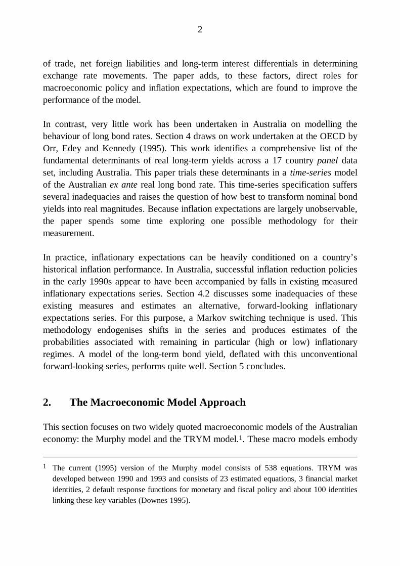
To better illustrate the relevant properties of the macroeconomic models, responsesto a domestic monetary policy shock and a terms of trade shock in the TRYMmodel are illustrated (Figures 1 and 2). 5
Firstly, a permanent 1 percentage point reduction in the exogenous money supply iseffected; this can be thought of as a standard textbook monetary policy tightening.Unfortunately, as described earlier, the macro model is not typically set up to dealwith an explicit interest rate shock. Such a simulation in TRYM would involvesuccessive manipulation of the money supply, producing ‘bumpy’ responsefunctions.
In the manner of forward-looking monetary models, the asset price variables ‘jump’instantaneously in reaction to any shock, typically exhibiting a damped
4 The term structure calculation is macro-model dependent. In the Murphy model, for example,
the yield on a 10-year security is set equal to the expected return from holding a continuoussequence of one-quarter securities over the next 10 years; the term premium is assumed to bezero. The expected returns from holding one-quarter securities are model consistent(Murphy 1988).
5 These results from the Treasury Macroeconomic (TRYM) model should in no way be regardedas being Treasury analyses of the effect of a given policy change or as having the sanction ofthe Treasury, the Treasurer or the Commonwealth Government.
7
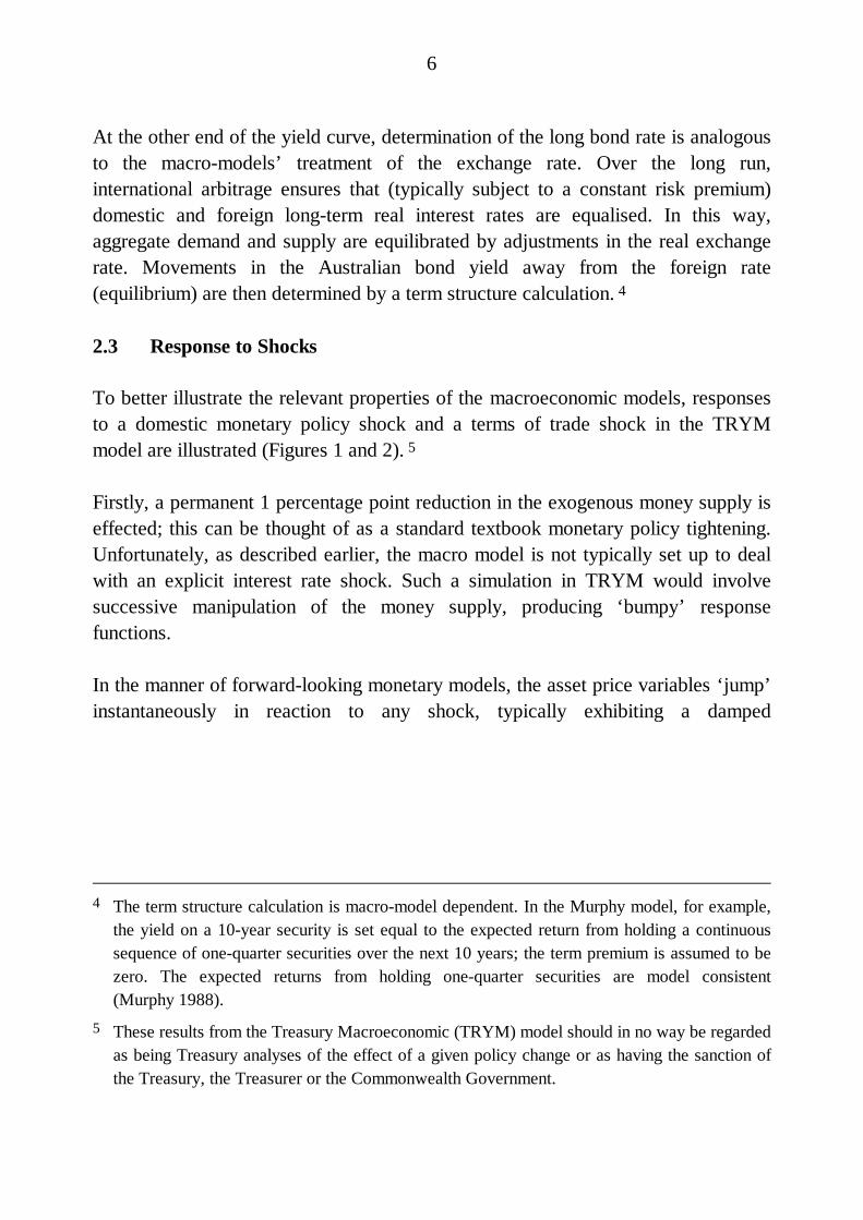
Figure 1: Money Supply ShockPermanent 1% Reduction
-0.3
0.0
0.3
0.6
-0.3
0
0.3
0.6
-0.3
0.0
0.3
0.6
-0.3
0.0
0.3
0.6
-0.5
0.0
0.5
1.0
-0.5
0.0
0.5
1.0
Real 90-day bank bill rate
Trade-weighted index
Nominal
Real
Real long interest rate
Inflation expectations
Real long interest rate andinflation expectations
Quarters from shock
0.90.9
Longrun
4 8 12 16 20 24 28 320
oscillation back to their long-run paths.6 A permanent 1 percentage pointcontraction of the money supply raises real short-term interest rates by 0.63 of apercentage point (Panel 1, Figure 1). This delivers a temporary fall-off in demandand a 1 percentage point reduction in the price level. The price fall is anticipatedand agents immediately reduce their inflationary expectations by 0.14 of apercentage point.
The nominal 10-year bond yield jumps up by 0.08 per cent in the initial quarter ofthe shock; through the uncovered interest parity (UIP) condition, the nominal
6 This long-run adjustment behaviour is largely due to the lagged adjustment processes
describing the demand side of the macro models.
8
exchange rate must depreciate by 0.08 of a percentage point per annum for the next10 years in order to equalise domestic and foreign returns. This requires animmediate appreciation of the exchange rate. Consistent with the imposedtheoretical condition of long-run money neutrality, the 1 per cent decrease in themoney supply has no effect on real variables in the long run, but leaves the nominalexchange rate appreciated by 1 percentage point.
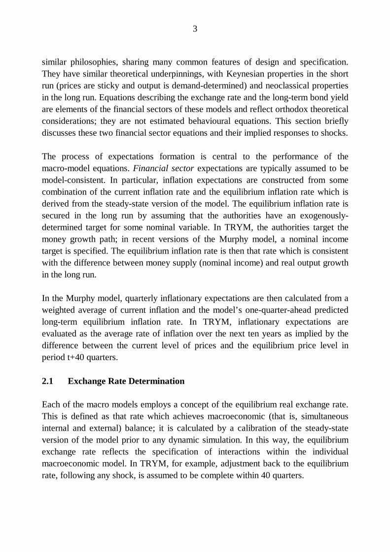
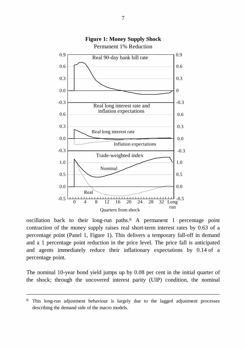
Alternatively, consider a sustained terms of trade shock, here effected through anincrease in the foreign price of exports that is maintained for ten quarters (Figure2).7 This shock raises domestic income. A proportion of the higher domestic incomeis spent on non-tradeable goods; this places upward pressure on prices and interestrates, appreciating the exchange rate via the UIP condition. The real exchange rateappreciates by around half of a percentage point.
If the shock had been permanent, the macro-model’s equilibrium exchange ratewould also have appreciated. This is because not all of the higher income arisingfrom a permanent increase in the terms of trade is spent on imports and the currentaccount balance improves; the macro-model’s equilibrium exchange rate must thenappreciate to generate a smaller trade surplus in the long run and thereby restoreexternal balance.
7 The shock is sustained over 10 quarters because this appears to be the average duration of
terms of trade shocks historically observed in the data.
9
Figure 2: Terms of Trade ShockSustained 1% Increase in Export Prices
-0.05
0.00
0.05
0.10
-0.05
0.00
0.05
0.10
Real long interest rate andinflation expectations
Real long interest rate
Inflation expectations
Trade-weighted index
-0.05
0.00
0.05
0.10
0.15
-0.05
0.00
0.05
0.10
0.15Real 90-day bank bill rate
Nominal
Real
-0.20
0.00
0.20
0.40
0.60
-0.20
0.00
0.20
0.40
0.60
0.20 0.20
Quarters from shock
Longrun
322824201612840
2.4 Assessment
The textbook-style impulse responses obtained from the macroeconomic models aredriven partly by the theoretical assumptions concerning financial market behaviouroutlined above. A number of critical points are worth highlighting.
• Within the macroeconomic model framework, the exchange rate and long bondyield display an instantaneous ‘jump’ response to shocks. This is usuallyfollowed by a damped oscillation to (partly) unwind the initial impulse.Experience suggests that such impulse responses do not accurately capture realworld dynamics.
10
• Inflationary expectations are also characterised as a ‘jump’ variable; theirinstantaneous response to shocks occurs before any adjustment in actualinflation. This feature of the macro-model approach does not line up closelywith actual experience. In many cases, a change in measured inflationaryexpectations has not occurred until after a change in actual inflation hasoccurred.
• Macro models are typically designed to produce policy simulations asresponses to shocks under one particular rule – a money-growth rule, forexample, in the case of TRYM. By contrast, policy simulations are morenaturally examined under alternative policy rules and in terms of changes in theshort-term interest rate.
• The size of the estimated exchange rate responses to terms of trade shockscannot comfortably accommodate the long-standing observed correlationbetween movements in the terms of trade and the Australian dollar (firstdocumented by Blundell-Wignall and Thomas (1987)).
• The assumption of UIP, embodying risk-neutrality (or a constant riskpremium), perfect capital mobility, efficiency in the foreign exchange market,and negligible transactions costs has no empirical support (Smith and Gruen(1989) for Australia; Goodhart (1988) and Hodrick (1987) for internationalevidence). Quite apart from the validity of the UIP assumption, which turns onthe issue of unbiasedness, predictions of future exchange rates based on UIPtend to be highly inaccurate.
With these points in mind, the remainder of this paper proceeds to develop simpler,single-equation behavioural models of the Australian exchange rate and long bondrate. This approach allows characterisation of the distinctive observed behaviour ofthese variables.
11
3. A Behavioural Model of the Australian Real Exchange Rate
3.1 What Determines the Australian Real Exchange Rate?
Previous empirical work (the most recent and comprehensive of which is Blundell-Wignall, Fahrer and Heath (1993), hereafter BW) has identified three statisticallysignificant determinants of the Australian real exchange rate:
• the terms of trade;
• net foreign liabilities (proxied by the cumulative current account deficit); and
• real long-term interest differentials.
Each of these is addressed in turn. Firstly, while all three ‘fundamentals’ have beenreported as statistically significant determinants of the real TWI exchange rate overthe period since the floating of the Australian dollar, only the terms of trade hasconsistently retained its explanatory power over a longer sample period (1973:Q2-1992:Q3). This latter result is consistent with the cross-country study of Amano andvan Norden (1992) which documents a robust relationship between the realdomestic price of oil and real effective exchange rates in Germany, Japan and theUnited States. They interpret the real oil price as capturing exogenous terms of tradeshocks and find these shocks to be the most important factor determining realexchange rates over the long run.
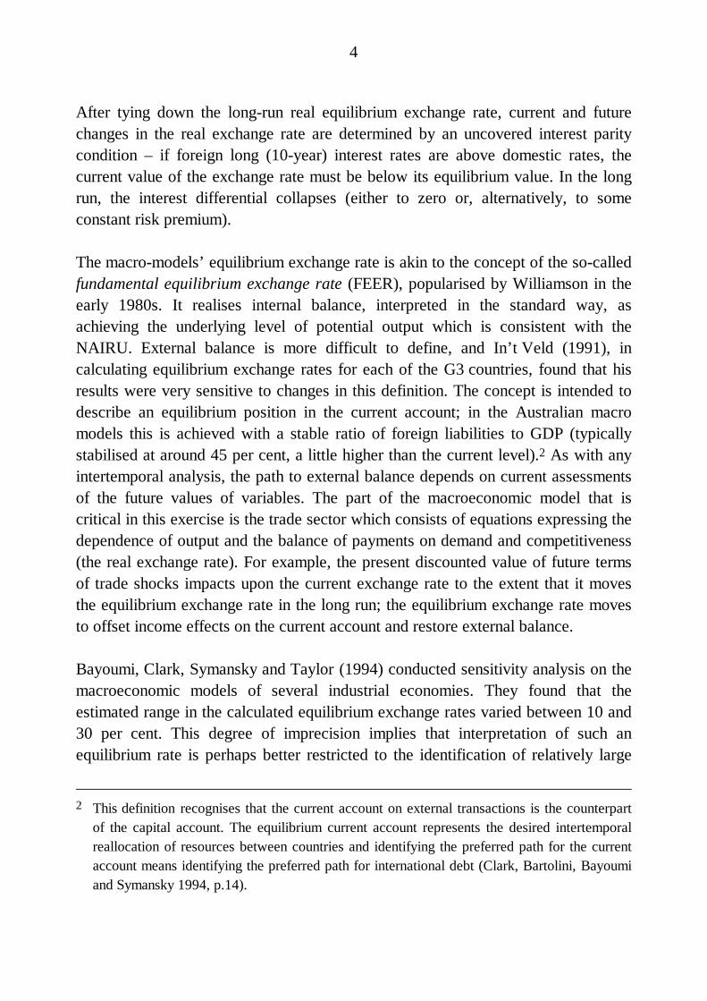
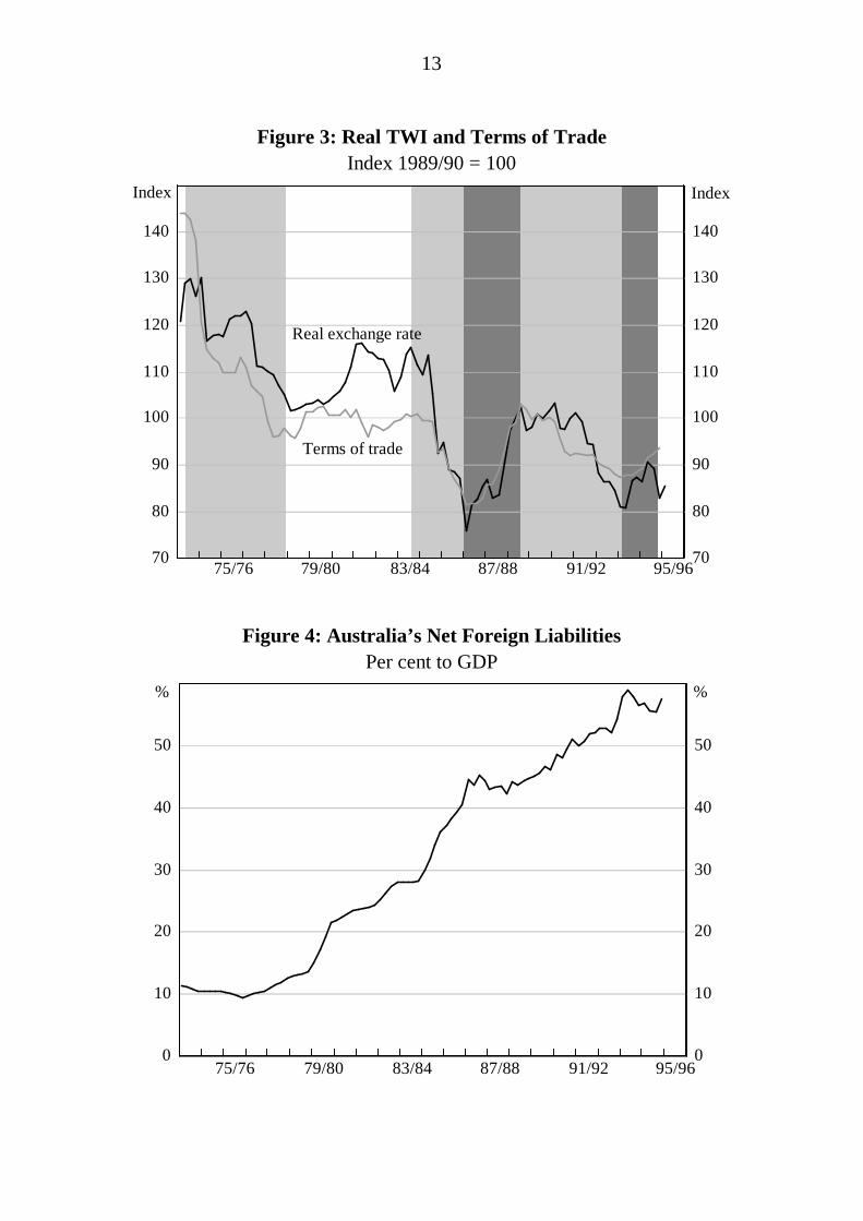
The relationship between the terms of trade and the Australian real exchange rate isstriking, as shown in Figure 3.8 Depreciations of the real TWI occurring in 1974-1978; 1984-1986; and 1991-1993 were all associated with falls in the terms of trade(denoted by the pale grey bars in Figure 3). Similarly, the real TWI appreciated over1987-1989 and 1994 when the terms of trade improved (highlighted by the darkergrey bars).
8 This is the terms of trade for goods and services. It seems reasonable to take the terms of trade
as exogenous because Australia’s share of world trade is small and it exports relatively fewdifferentiated products. Dwyer, Kent and Pease (1994) present empirical evidence forAustralia.
12
An exception can be identified in the early 1980s. This period coincides with aresources investment boom, promoted by the second OPEC oil-price shock andprovides a good example of the role that expectations can play in determiningmovements in the exchange rate. The resources boom generated optimisticexpectations about future improvements in the terms of trade and thereby, futureincome; the TWI appreciated despite little change in the prevailing terms of trade.Given that the anticipated improvements never eventuated, a correction inexpectations contributed to the magnitude of the real TWI depreciation over 1985and the first half of 1986.
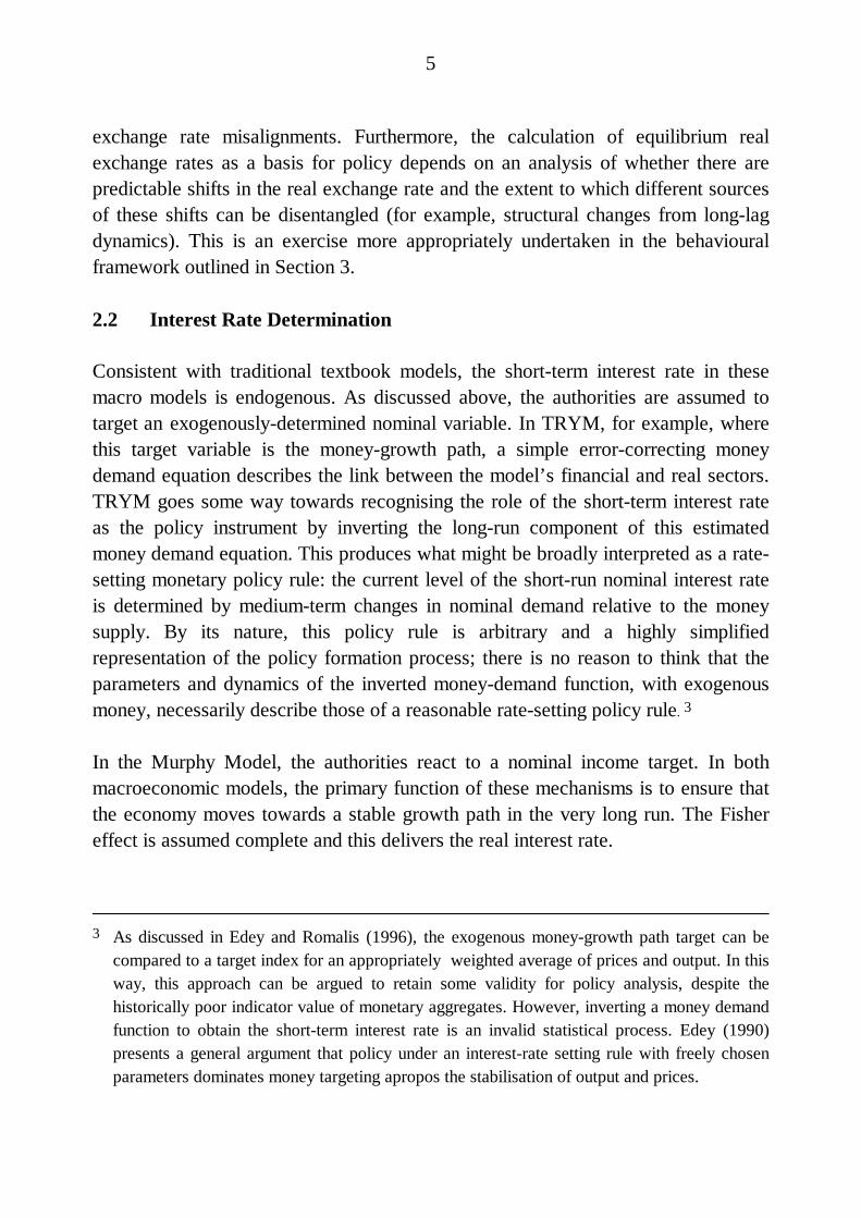
Secondly, Australia experienced a rapid and sustained rise in net foreign liabilitiesover the 1980s (Figure 4).9 Increasing net foreign liabilities, as a share of wealth,require larger balance of trade surpluses to restore equilibrium.
Similar to the macro-model mechanism of maintaining external balance, this mayrequire a depreciation of the real exchange rate to attract resources into thetradeables sector. (Of course, if the real return on investment is high, the highertrade surpluses may be achieved without a real depreciation.)
Thirdly, the vast majority of the literature finds that the long-term real interestdifferential has the most success in obtaining significant and correctly signedestimates in exchange rate equations (Gruen and Wilkinson (1991) and BW forAustralia; Isard (1988) and Shafer and Loopesko (1983) for international evidence).Long-term interest differentials are often justified on the grounds that shocks to thereal exchange rate can persist for long periods and this slow reversion towardsequilibrium is simply more appropriately matched by a correspondingly long-terminterest rate.10 This seems curious given that the
9 Empirical work generally uses the cumulated current account deficit as a proxy for net foreign
liabilities because it abstracts from valuation effects.
10 Isard (1983) supports the use of long (10-year) interest rate differentials on the grounds thatthey are convenient to interpret. As in the Australian macro models, he assumes that theexpected real exchange rate in 10 years time is the equilibrium exchange rate; in this way, thelong (10-year) real interest differential (corrected for any risk premium) can be interpreted asdenoting the annual rate of real depreciation/appreciation of the dollar expected by the marketover the next 10 years.
13
Figure 3: Real TWI and Terms of TradeIndex 1989/90 = 100
70
80
90
100
110
120
130
140
70
80
90
100
110
120
130
140
Index
Real exchange rate
Terms of trade
Index
95/9691/9287/8883/8479/8075/76
Figure 4: Australia’s Net Foreign LiabilitiesPer cent to GDP
0
10
20
30
40
50
0
10
20
30
40
50
%
95/9691/9287/8883/8479/8075/76
%
14
exchange rate is considered to be an important channel through which changes inthe policy-determined short-term interest rate feed through to the economy.De Kock and Deleire (1994) estimate that, post 1982 in the United States, theexchange rate accounts for roughly one-third of monetary policy transmission tooutput, compared to a near-negligible contribution earlier. Perhaps it is the case thatearlier Australian studies did not have the benefit of a sufficiently long sampleperiod, after the floating of the Australian dollar, over which to estimate theirexchange rate models. At any rate, this seems to beg further investigation.
The real long-term interest differential in existing models could simply be replacedby a real short-term interest differential. As customarily measured – using 12-months-ended inflation rates – real short-term interest rate differentials would reflectthe prevailing stance of domestic, relative to foreign, monetary policy; but theywould fail to capture any market anticipation of the future paths of short-terminterest rates, inflation and growth.
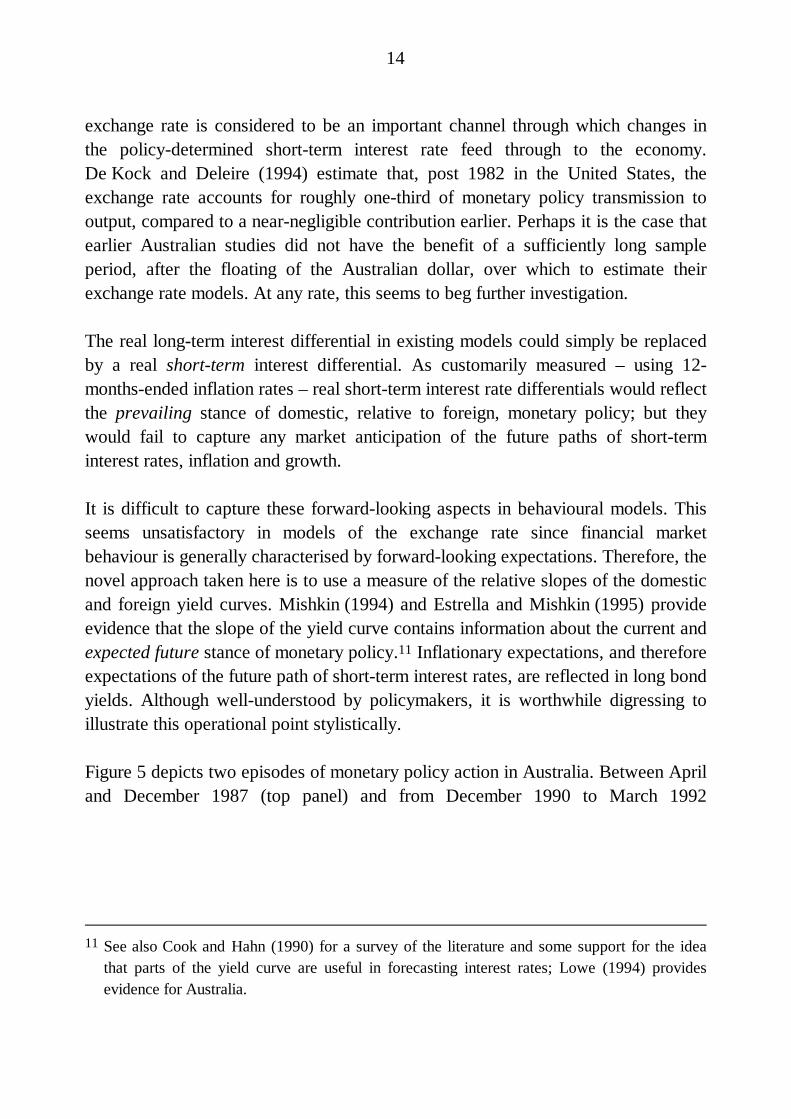
It is difficult to capture these forward-looking aspects in behavioural models. Thisseems unsatisfactory in models of the exchange rate since financial marketbehaviour is generally characterised by forward-looking expectations. Therefore, thenovel approach taken here is to use a measure of the relative slopes of the domesticand foreign yield curves. Mishkin (1994) and Estrella and Mishkin (1995) provideevidence that the slope of the yield curve contains information about the current andexpected future stance of monetary policy.11 Inflationary expectations, and thereforeexpectations of the future path of short-term interest rates, are reflected in long bondyields. Although well-understood by policymakers, it is worthwhile digressing toillustrate this operational point stylistically.
Figure 5 depicts two episodes of monetary policy action in Australia. Between Apriland December 1987 (top panel) and from December 1990 to March 1992
11 See also Cook and Hahn (1990) for a survey of the literature and some support for the idea
that parts of the yield curve are useful in forecasting interest rates; Lowe (1994) providesevidence for Australia.
15
Figure 5: Episodes of Policy Change
-4
-2
0
-4
-2
0
-6
-4
-2
0
-6
-4
-2
0
Change from 10 April 1987
Change from 18 December 1990
10-year bond
10-year bond
Cash rate
Cash rate
543210
%pts
%pts
%pts
%pts
-1Quarters from policy change represented on horizontal axis
(bottom panel), the operational instrument of monetary policy in Australia – thenominal cash rate – was reduced by around 5 1
2 percentage points.
In the first episode, in 1987, the long bond yield remained relatively unchanged(falling by a small 0.48 of a percentage point). By comparison, over the early 1990sepisode, the long bond yield fell by almost 4 percentage points. At this time, someprogress on inflation was already widely apparent in Australia and so marketexpectations for future inflation may well have moderated with the reduction in thecash rate. Of course, this discussion is simplistic and ignores a number of issues, butto the extent that inflation expectations explain some of the fall in the long end ofthe yield curve, agents were not expecting short-rates to have to rise very much inthe future. Relative to the example in 1987, the slope of the yield curve remainedfairly flat. By this measure, the stance of monetary policy was relatively tighter than
16
over the 8 months to December 1987, despite equivalent movements in the nominalcash rate.
Also of interest to policymakers is the role of fiscal policy in determining exchangerate behaviour. Rarely mentioned in earlier work on the Australian exchange rate,the impact of fiscal policy can occur through two separate channels and istheoretically ambiguous.
• Firstly, the simplest Mundell-Fleming model predicts that expansionary fiscalpolicy causes an appreciation of the exchange rate. The intuition for this resultis that increased government spending raises demand for domestic outputwhich, in turn, induces a currency appreciation (alternatively, increaseddemand exerts upward pressure on interest rates which induces capital inflowand a stronger currency). The appreciated currency reduces the value offoreign demand, which restores the original level of output.
• Secondly, fiscal policy can impact upon the exchange rate through a riskpremium. Fiscal expansion may be penalised by investors who perceive anincreased probability of default or expect higher inflation in the future becausethey believe that the incentive exists for the Government to ‘inflate’ its debtaway; in order to hold Australian dollar assets, they demand a risk premium ondomestic interest rates. Furthermore, it is often argued that higher governmentbudget deficits are associated with negative sentiment on the exchange ratebecause they imply lower national savings and so greater net foreign liabilitiesin the longer run. In this way, it is argued that the exchange rate depreciates.To the extent that the negative sentiment arises because of the overall size ofnet foreign liabilities, rather than their public/private composition, this effectmay be partly captured, over the long run, by a cumulated current accountvariable.
Both the monetary and fiscal policy variables discussed above seem likely to beimportant, in addition to the variables identified in earlier work, for explainingmovements in the Australian real exchange rate. To ascertain the empirical validityof this proposition, the BW equation, being the most recent in this literature, istested for and appears to suffer from omitted variable bias.
17
Table 1: Omitted Variable Tests
Estimation period RESET Rainbowtest
Significance level
1984:Q1-1992:Q3(BW 1993)
3.11** F(18,10): 0.035
1984:Q1-1995:Q2(Updated BW sample)
2.61** F(24,16): 0.026
1985:Q1-1995:Q2(Tarditi 1996)
2.02* F(22,14): 0.089
Notes: ** and * denote rejection of the null hypothesis of no omitted variables at the 5% and10% significance level.
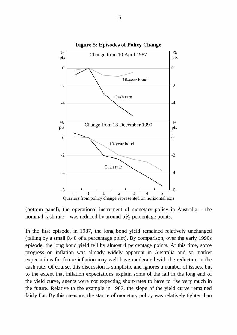
Table 1 summarises the results from application of the ‘rainbow test’, a member ofthe Ramsey (1969) RESET family of tests for the omission of unknown variables(Utts 1982).12 The test is conducted over several post-float sample periods, whenthe exchange rate became a channel of transmission for monetary policy; the nullhypothesis of no omitted variables is consistently rejected. The omitted variable(s)will be captured in the error process and as a consequence, the estimatedcoefficients in the BW equation will be both biased and inconsistent.
In an effort to address this bias, several modifications to the BW specification aremade. Specifically, the terms of trade and cumulated current account deficit areretained. A yield gap differential replaces the long-term interest differential andtakes the form:
YGAP = (is{ − iL ) − (is − iL )*} (1)
12 The ‘rainbow test’ compares estimates of the variance of the regression disturbance obtained
from estimation over the relevant full sample and a truncated sub-sample; if the null hypothesisis true, both variance estimates are unbiased. The test statistic is an F-statistic, adjusted for theappropriate degrees of freedom. See Kmenta (1990, pp.454-455) for a full description of thetest. It should be noted that the consequences of omitting relevant explanatory variables are thesame as those of using an incorrect functional form.
18
where:
(is − iL ) measures the slope of the domestic yield curve as the differencebetween the domestic nominal cash rate (is) and the domesticnominal long (10 year) bond yield (iL ) ;
(is − iL )* measures the slope of the foreign yield curve using equivalentforeign interest rates (see Appendix A for details on the constructionof world interest rates and Table B.2 in Appendix B for statisticalconfirmation of the implied restrictions in (1)).
In addition, a role for fiscal policy is accommodated by including a measure of thechange in the Commonwealth Government budget balance, expressed as aproportion of GDP (hereafter, the fiscal variable). While it would be preferable touse a cyclically-adjusted measure of the fiscal position, this was not available forAustralia.13
3.2 The Empirical Results
Following the convention for time series methodology, the order of integration ofthe real exchange rate and its proposed explanatory variables is established (seeTable B.3 in Appendix B for detailed statistics). To this end, the AugmentedDickey-Fuller (Dickey and Fuller 1981; Said and Dickey 1984) and Elliot,Rothenberg and Stock (1992) (DF-GLS) tests of a unit root null, together with theKwiatkowski, Phillips, Schmidt and Shin (1992) (KPSS) test of a stationary (trendstationary) null, are employed.14 Confirming the results of Bleaney (1993) and
13 Typically, the government budget tends to be in surplus when the economy is growing strongly
and vice versa. The fiscal variable was tested against domestic and foreign growth variablesand measures of the output gap to eliminate the possibility that it was just proxying theeconomic cycle. The fiscal variable retained its explanatory power over both the shorter post-float period (1985:Q1-1995:Q2) and the longer, historical sample period (1973:Q4-1995:Q2).These results were not qualitatively altered when the Commonwealth Government measure ofthe fiscal position was replaced by a measure of the change in the public sector borrowingrequirement.
14 The null hypothesis of a unit root in the ADF and DF-GLS tests may result in a type II error;series may appear to contain a unit root because the data are insufficient to provide strong
19
Gruen and Kortian (1996), these tests imply mean reversion of the Australian realexchange rate to a slowly declining trend.15 Similar evidence of stationarity existsfor other countries (see, for example, Phylaktis and Kassimatis (1994); Liu and He(1991) and Huizinga (1987)).16 The integration tests also provide evidence that theterms of trade and other explanatory variables are I(0) processes.
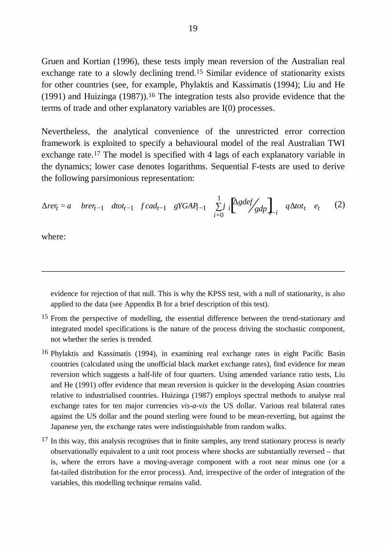
Nevertheless, the analytical convenience of the unrestricted error correctionframework is exploited to specify a behavioural model of the real Australian TWIexchange rate.17 The model is specified with 4 lags of each explanatory variable inthe dynamics; lower case denotes logarithms. Sequential F-tests are used to derivethe following parsimonious representation:
∆rert = α + βrert − 1 + δtott − 1 + φcadt− 1 + γYGAPt − 1 + ϕ ii=0
1∑ ∆gdef
gdp[ ]t− i+ θ∆tott + εt (2)
where:
evidence for rejection of that null. This is why the KPSS test, with a null of stationarity, is alsoapplied to the data (see Appendix B for a brief description of this test).
15 From the perspective of modelling, the essential difference between the trend-stationary andintegrated model specifications is the nature of the process driving the stochastic component,not whether the series is trended.
16 Phylaktis and Kassimatis (1994), in examining real exchange rates in eight Pacific Basincountries (calculated using the unofficial black market exchange rates), find evidence for meanreversion which suggests a half-life of four quarters. Using amended variance ratio tests, Liuand He (1991) offer evidence that mean reversion is quicker in the developing Asian countriesrelative to industrialised countries. Huizinga (1987) employs spectral methods to analyse realexchange rates for ten major currencies vis-a-vis the US dollar. Various real bilateral ratesagainst the US dollar and the pound sterling were found to be mean-reverting, but against theJapanese yen, the exchange rates were indistinguishable from random walks.
17 In this way, this analysis recognises that in finite samples, any trend stationary process is nearlyobservationally equivalent to a unit root process where shocks are substantially reversed – thatis, where the errors have a moving-average component with a root near minus one (or afat-tailed distribution for the error process). And, irrespective of the order of integration of thevariables, this modelling technique remains valid.
20
rer Australian real TWI exchange rate;
tot terms of trade;
cad cumulated current account deficit, expressed as a proportion of GDP(defined such that a current account deficit is a positive number);
YGAP relative slopes of domestic and foreign yield curves as described in(1) above (see Table B.2 in Appendix B for statistical confirmationof the implied interest rate restrictions);
∆gdefgdp fiscal variable, defined as the log change in the Commonwealth
Government deficit and expressed as a proportion of GDP (definedsuch that a budget deficit is a positive number);
ε white noise error term;
∆ first difference operator.
Given the time-series properties of the data, this specification is used to distinguishdifferent types of influences on the real exchange rate and, in this way, retains onecharacteristic of the macroeconomic models described in Section 2 – namely, thegeneral framework wherein the real exchange rate – affected by speculative andcyclical factors – eventually tends toward a path determined by underlying structuralfactors. The macroeconomic fundamentals, identified in Section 3.1 above, set theparameters within which the exchange rate should move in the medium term andprovide a pertinent framework from which to assess the appropriateness of policysettings.
The model is estimated over two sample periods; three decades of data encompasstwo broad exchange rate regimes in which the dynamics of the real exchange rateare unlikely to be identical. With this in mind, results for equation (2) over the post-
21
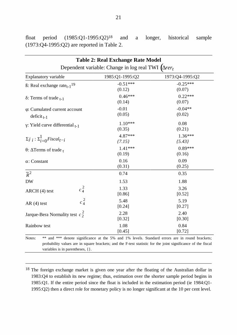
float period (1985:Q1-1995:Q2)18 and a longer, historical sample(1973:Q4-1995:Q2) are reported in Table 2.
Table 2: Real Exchange Rate ModelDependent variable: Change in log real TWI ∆rert( )
Explanatory variable 1985:Q1-1995:Q2 1973:Q4-1995:Q2
ß: Real exchange ratet-119 -0.51***(0.12)
-0.25***(0.07)
δ: Terms of trade t-1 0.46***(0.14)
0.22***(0.07)
φ: Cumulated current account deficit t-1
-0.01(0.05)
-0.04**(0.02)
γ: Yield curve differential t-1 1.10***(0.35)
0.08(0.21)
Σϕi : Σi=01 Fiscalt− i
4.87***{7.15}
1.36***{5.43}
θ: ∆Terms of trade t 1.41***(0.19)
0.89***(0.16)
α: Constant 0.16(0.31)
0.09(0.25)
R2 0.74 0.35
DW 1.53 1.88
ARCH (4) test χ42 1.33
[0.86]3.26
[0.52]
AR (4) test χ42 5.48
[0.24]5.19
[0.27]
Jarque-Bera Normality test χ22 2.28
[0.32]2.40
[0.30]Rainbow test 1.08
[0.45]0.84
[0.72]Notes: ** and *** denote significance at the 5% and 1% levels. Standard errors are in round brackets;
probability values are in square brackets; and the F-test statistic for the joint significance of the fiscalvariables is in parentheses, {}.
18 The foreign exchange market is given one year after the floating of the Australian dollar in
1983:Q4 to establish its new regime; thus, estimation over the shorter sample period begins in1985:Q1. If the entire period since the float is included in the estimation period (ie 1984:Q1-1995:Q2) then a direct role for monetary policy is no longer significant at the 10 per cent level.

22
Three points are worth noting straight away.
• As expected, it is only after the floating of the Australian dollar that theexchange rate has played a role in channelling changes in real interest ratesthrough to the broader economy.20
• On the other hand, the cumulated current account deficit is only significant inexplaining the real exchange rate over the fuller, historical sample period; thisaccords with its longer-run structural nature.21 Over this period, the level ofAustralia’s net foreign liabilities is estimated to have exerted some downwardpressure on the real exchange rate, but this has been of a relatively small orderof magnitude; a one percentage point increase in net foreign liabilities to GDP,ceteris paribus, has an estimated long run effect of 1/6 of a percentage point onthe real exchange rate over this period.
• The positive coefficient on the fiscal policy variable implies a conventionally-signed Mundell-Flemming effect during the sample period.
The remainder of this section concentrates on interpretation of the results obtainedfrom estimation of this model over the post-float period. Simple impulse responsediagrams show the estimated impact of shocks to the yield curve and to the terms oftrade, ceteris paribus, on the real exchange rate.
The first shock is defined as a one percentage point inversion of the Australian yieldcurve relative to the foreign yield curve, maintained for eight quarters. In response,the real exchange rate is estimated to appreciate by 2.2 percentage points; 76 percent of the adjustment is complete after two quarters (Figure 6a). This gradual
19 β measures the speed of adjustment which, for the post-float regression, implies a half life of1 quarter; this is not unreasonable given that the real exchange rate is trend stationary.
20 It is worth noting that the relative yield gap variable outperforms (statistically) the alternativeshort-term real interest differential over this sample period (see Table B.4 in Appendix B fordetails).
21 This is the opposite of the BW result that the cumulated current account deficit is onlysignificant over the shorter, post-float sample period and even then, that it is outperformed bya simple trend (see Table B.1 in Appendix B).
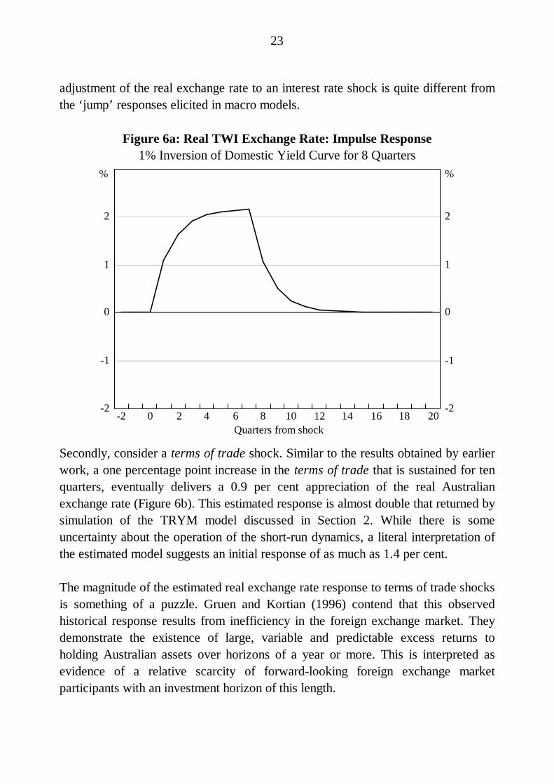
23
adjustment of the real exchange rate to an interest rate shock is quite different fromthe ‘jump’ responses elicited in macro models.
Figure 6a: Real TWI Exchange Rate: Impulse Response1% Inversion of Domestic Yield Curve for 8 Quarters
-2
-1
0
1
2
-2
-1
0
1
2
% %
Quarters from shock20181614121086420-2
Secondly, consider a terms of trade shock. Similar to the results obtained by earlierwork, a one percentage point increase in the terms of trade that is sustained for tenquarters, eventually delivers a 0.9 per cent appreciation of the real Australianexchange rate (Figure 6b). This estimated response is almost double that returned bysimulation of the TRYM model discussed in Section 2. While there is someuncertainty about the operation of the short-run dynamics, a literal interpretation ofthe estimated model suggests an initial response of as much as 1.4 per cent.
The magnitude of the estimated real exchange rate response to terms of trade shocksis something of a puzzle. Gruen and Kortian (1996) contend that this observedhistorical response results from inefficiency in the foreign exchange market. Theydemonstrate the existence of large, variable and predictable excess returns toholding Australian assets over horizons of a year or more. This is interpreted asevidence of a relative scarcity of forward-looking foreign exchange marketparticipants with an investment horizon of this length.

24
Figure 6b: Real TWI Exchange Rate: Impulse ResponseSustained 1% Terms of Trade Shock
-2 0 2 4 6 8 10-0.3
0.0
0.3
0.6
0.9
1.2
-0.3
0.0
0.3
0.6
0.9
1.2
%%
Quarters from shock
If this myopic behaviour does indeed prevail, participants in the foreign exchangemarket may not be adequately distinguishing between temporary,soon-to-be-reversed shocks and longer, more sustained shifts in the terms of trade.This would result in Australia’s real exchange rate moving more tightly with theterms of trade than would be consistent with perfectly forward-looking investorbehaviour. While the smaller responses to temporary terms of trade shocksgenerated by the macro models is theoretically appealing, the presence of excessreturns in the foreign exchange market undermines the predictions of UIP; thiscondition is the central relationship determining exchange rate outcomes in themacro models.
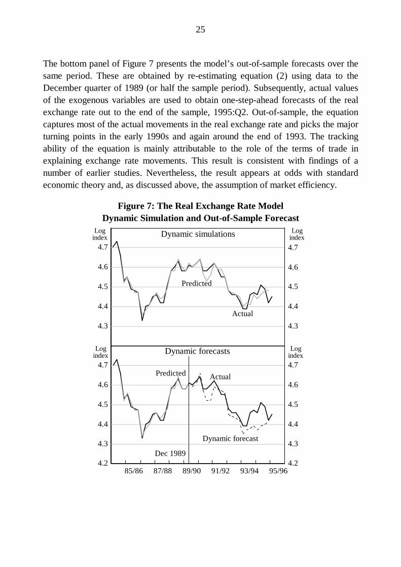
To give some idea of the model’s fit, Figure 7 compares the actual behaviour of thereal Australian TWI exchange rate over the post-float period, with predicted valuesfrom this model up to the June quarter of 1995. In sample, the model fits very well.
25
The bottom panel of Figure 7 presents the model’s out-of-sample forecasts over thesame period. These are obtained by re-estimating equation (2) using data to theDecember quarter of 1989 (or half the sample period). Subsequently, actual valuesof the exogenous variables are used to obtain one-step-ahead forecasts of the realexchange rate out to the end of the sample, 1995:Q2. Out-of-sample, the equationcaptures most of the actual movements in the real exchange rate and picks the majorturning points in the early 1990s and again around the end of 1993. The trackingability of the equation is mainly attributable to the role of the terms of trade inexplaining exchange rate movements. This result is consistent with findings of anumber of earlier studies. Nevertheless, the result appears at odds with standardeconomic theory and, as discussed above, the assumption of market efficiency.
Figure 7: The Real Exchange Rate ModelDynamic Simulation and Out-of-Sample Forecast
4.3
4.4
4.5
4.6
4.7
4.3
4.4
4.5
4.6
4.7
85/86 87/88 89/90 91/92 93/94 95/964.2
4.3
4.4
4.5
4.6
4.7
4.2
4.3
4.4
4.5
4.6
4.7
Dynamic forecasts
Dynamic simulations
Dec 1989
Logindex
Logindex
Logindex
Logindex
Dynamic forecast
ActualPredicted
Actual
Predicted
26
4. A Behavioural Model of the Australian Long-Term InterestRate
In contrast to the volume of literature on determinants of the exchange rate, work onmodelling the behaviour of the Australian long bond rate is scarce. This section ofthe paper draws on recent work undertaken at the OECD by Orr et al., who identifya comprehensive list of the fundamental determinants of real long-term interest ratesacross a 17-country panel data set, including Australia. The authors also provide asuccinct yet comprehensive discussion of each of these determinants. Thisdiscussion will not be repeated here. Instead, by using the ‘fundamental’ variablesidentifed by Orr et al., a time-series equation for the Australian ex ante real longbond rate is trialed.
This time-series specification suffers several inadequacies and raises the question ofhow best to transform nominal bond yields into real magnitudes. Since inflationexpectations are largely unobservable, Section 4.2 of the paper spends some timeexploring one possible methodology for their measurement. Estimation of a simplemodel of inflation, specified to endogenise shifts between a high and a low inflationregime, is used to generate forward-looking expectations. This methodology seemsparticularly apt for Australia, where successful inflation reduction policies in theearly 1990s have been accompanied by a discrete shift in existing survey measuresof inflationary expectations. The explanatory performance of this unconventionalforward-looking measure is compared to an existing survey measure of inflationaryexpectations in a time-series model of nominal long bond rates.
4.1 The Real Bond Yield Fundamentals in Brief
I begin with the principle determinants of real long bond yields. Orr et al. list thesedeterminants as the domestic rate of return on capital, the world real long bondyield, and various risk premia. They note that these risk premia are likely to dependon:
• the perceived degree of each country’s monetary policy commitment to pricestability. Recognising that the expectations of market participants may followsome adaptive process, they use the existing level of inflationary expectations,conditioned on some longer-run historical performance (the average rate ofinflation over the preceding 10 years, π 10 ). In this way, movements in bond
27
yields relative to changes in current inflationary expectations will depend onthe weight that investors attribute to Australia’s relatively poorer historicalinflation performance;
• the expected sustainability of government fiscal and net external debt positions.Orr et al. measure these with the ratios of government budget positions andcumulated current account deficits, respectively, to GDP; and
• some undiversifiable domestic portfolio risk associated with holding bonds.22
Following the time-series methodology outlined in Section 3, the real long bondyield, r, deflated simply, first of all, with (annualised) quarterly underlying inflationrates, is determined by an unrestricted error correction model.23 Tests of the orderof integration of each variable are presented in Table C.1 in Appendix C. Four lagsof each of the differenced ‘fundamental’ variables, together with domestic growth,were included in the initial dynamic specification of the model; F-tests were thenused to derive the parsimonious final model:
∆rt = αrt− 1 + β π 10 − Et (π ){ }+ γ0 RetCapt − 1 + σ∆rt − 2 + φ∆ RetCapt− 1 +
λ0∆Et (π ) + λ2∆Et− 2 (π) + θ∆GDeft + gt − ii=0
1∑ + εt
(3)
where:rt real Australian 10-year bond yield, deflated with annualised
quarterly underlying inflation rates;π 10 the average rate of inflation over the preceding 10 years;Et(π ) current inflationary expectations, generated by a Hodrick-Prescott
filter of the GDP deflator;RetCap return on capital, measured as in Orr et al., as the ratio of gross
operating surplus of private corporate trading enterprises to thatsector’s capital stock;
22 It may also be the case that some degree of liquidity risk exists for Australia, due to a relatively
shallow bond market. It is reasonable to expect that this risk is declining over time as themarket matures and deepens.
23 Annualised quarterly inflation rates are used to avoid the introduction of autocorrelation.
28
GDef Commonwealth Government Budget deficit, expressed as aproportion of GDP (a deficit is denoted as a positive number);
g domestic GDP growth, measured with the four-quarter-ended growthrate of GDP;
εt white noise error term;∆ difference operator.
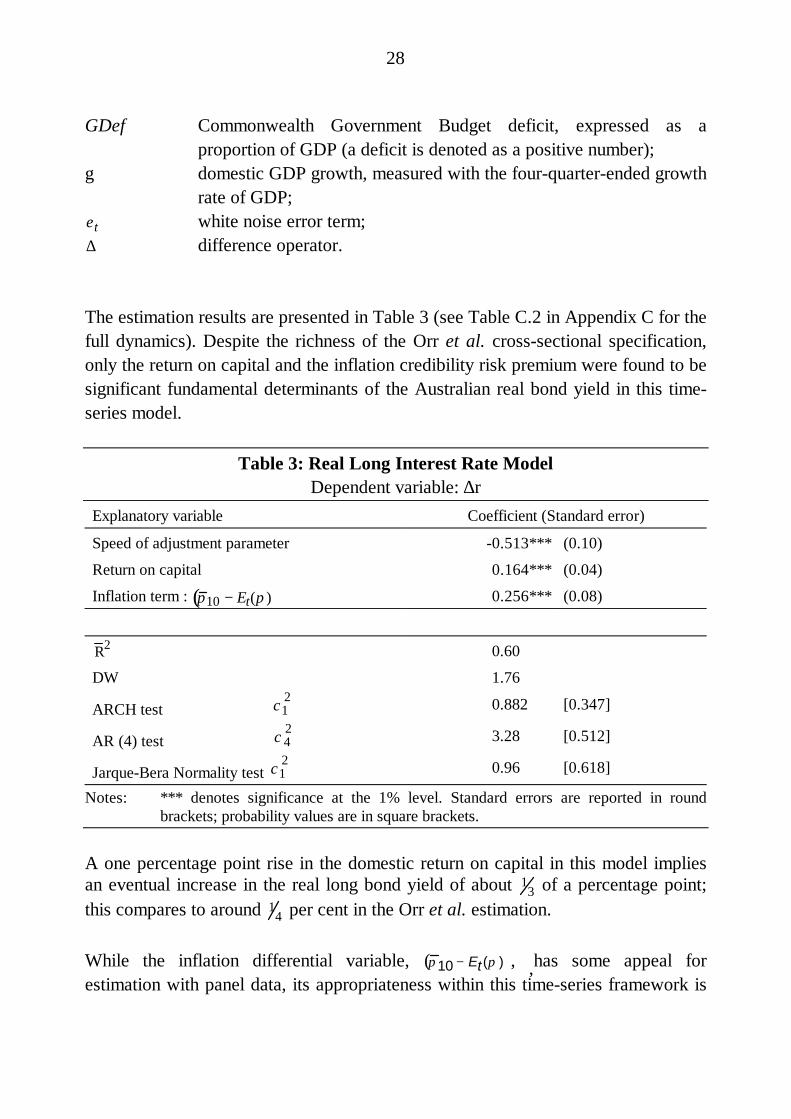
The estimation results are presented in Table 3 (see Table C.2 in Appendix C for thefull dynamics). Despite the richness of the Orr et al. cross-sectional specification,only the return on capital and the inflation credibility risk premium were found to besignificant fundamental determinants of the Australian real bond yield in this time-series model.
Table 3: Real Long Interest Rate ModelDependent variable: ∆r
Explanatory variable Coefficient (Standard error)
Speed of adjustment parameter -0.513*** (0.10)
Return on capital 0.164*** (0.04)
Inflation term : π 10 − Et(π)( ) 0.256*** (0.08)
R 2 0.60
DW 1.76
ARCH test χ12 0.882 [0.347]
AR (4) test χ42 3.28 [0.512]
Jarque-Bera Normality test χ12 0.96 [0.618]
Notes: *** denotes significance at the 1% level. Standard errors are reported in roundbrackets; probability values are in square brackets.
A one percentage point rise in the domestic return on capital in this model impliesan eventual increase in the real long bond yield of about 1
3 of a percentage point;this compares to around 1
4 per cent in the Orr et al. estimation.
While the inflation differential variable, π 10 − E t ( π ) ( ) , ,has some appeal forestimation with panel data, its appropriateness within this time-series framework is
29
difficult to justify. This is because, by construction, the real bond yield will often berelatively high in periods when the current (expected) rate of inflation is low; thiswill also be true of the inflation variable. That is, the existence of some meanreversion in inflation would generate this positive, significant coefficient on theinflation differential variable.
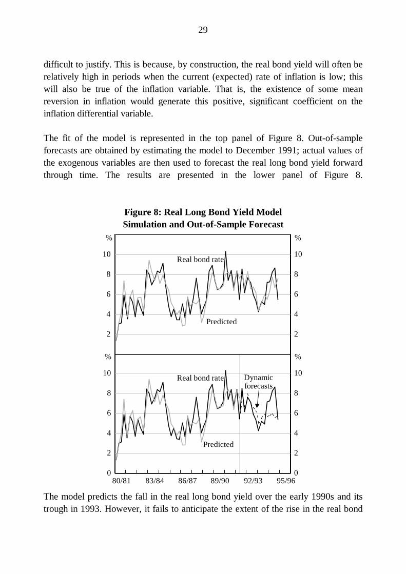
The fit of the model is represented in the top panel of Figure 8. Out-of-sampleforecasts are obtained by estimating the model to December 1991; actual values ofthe exogenous variables are then used to forecast the real long bond yield forwardthrough time. The results are presented in the lower panel of Figure 8.
Figure 8: Real Long Bond Yield ModelSimulation and Out-of-Sample Forecast
2
4
6
8
10
2
4
6
8
10Real bond rate
Dynamicforecasts
%%
80/81 83/84 86/87 89/90 92/93 95/960
2
4
6
8
10
0
2
4
6
8
10
Predicted
Real bond rate
%%
Predicted
The model predicts the fall in the real long bond yield over the early 1990s and itstrough in 1993. However, it fails to anticipate the extent of the rise in the real bond
30
yield over the course of 1994, suggesting, perhaps, that the world-wide bond marketsell-off was not completely consistent with fundamentals. Despite the fact that asimilar pattern was documented in most OECD countries over 1994, the panelestimation in Orr et al. also fails to predict bond yield behaviour over this period.
Given the reservations with the model’s (likely spurious) dependence on theinflation differential term, π 10 − E t ( π ) ( ) , it may be the case that the dependentvariable, measured as it is, with backward-looking inflationary expectations, is notan adequate measure of the ex ante real long bond yield. The remainder of thissection concentrates on one alternative method of constructing a forward-lookingmeasure of inflation expectations for inclusion in a model of Australian long bondyields.
4.2 Measuring Inflationary Expectations
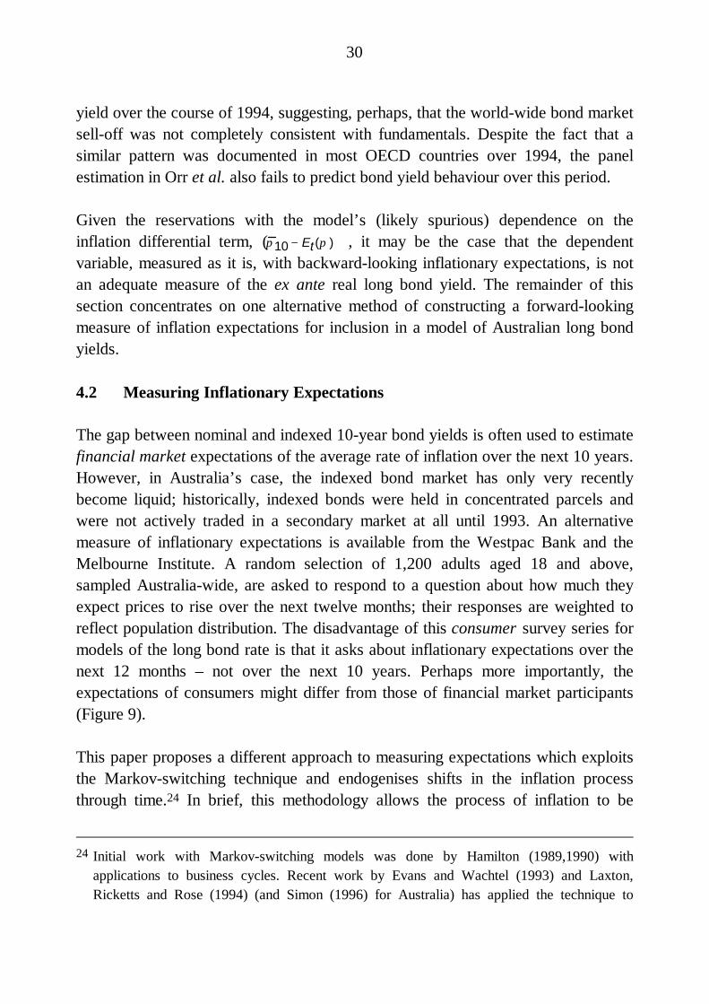
The gap between nominal and indexed 10-year bond yields is often used to estimatefinancial market expectations of the average rate of inflation over the next 10 years.However, in Australia’s case, the indexed bond market has only very recentlybecome liquid; historically, indexed bonds were held in concentrated parcels andwere not actively traded in a secondary market at all until 1993. An alternativemeasure of inflationary expectations is available from the Westpac Bank and theMelbourne Institute. A random selection of 1,200 adults aged 18 and above,sampled Australia-wide, are asked to respond to a question about how much theyexpect prices to rise over the next twelve months; their responses are weighted toreflect population distribution. The disadvantage of this consumer survey series formodels of the long bond rate is that it asks about inflationary expectations over thenext 12 months – not over the next 10 years. Perhaps more importantly, theexpectations of consumers might differ from those of financial market participants(Figure 9).
This paper proposes a different approach to measuring expectations which exploitsthe Markov-switching technique and endogenises shifts in the inflation processthrough time.24 In brief, this methodology allows the process of inflation to be
24 Initial work with Markov-switching models was done by Hamilton (1989,1990) with
applications to business cycles. Recent work by Evans and Wachtel (1993) and Laxton,Ricketts and Rose (1994) (and Simon (1996) for Australia) has applied the technique to
31
characterised by two different regimes, the first identified by relatively highinflation; the second, by relatively low inflation. Switches between these states arebased on a probabilistic process.25 Maximum likelihood estimation of the two-statemodel returns a probability that inflation is in one or other of these regimes. This isused to construct a probability-weighted n-period-ahead inflationary expectationsseries which is, by its nature, forward looking. Thus constructed, this series is foundto be superior to its survey alternative in a model of the nominal bond yield (Section4.3).
Figure 9: Measures of Inflationary Expectations
2
4
6
8
10
2
4
6
8
10
Survey of consumerexpectations
Financial market expectations(Nominal less indexed bond yield)
95/9693/9491/9289/9087/8885/86
% %
inflation with a view to examining the issue of central bank credibility. The Gauss programmeused for estimation of the Markov switching model is an adaption of that used by Hamilton(1989) and Goodwin (1993) and I thank Thomas Goodwin for generously providing me withthe computor code.
25 A Markov process is one where the (fixed) probability of being in a particular state is onlydependent upon what the state was last period.
32
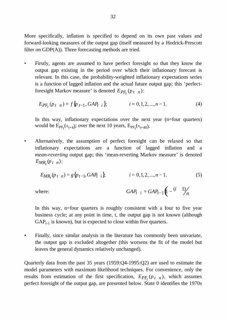
More specifically, inflation is specified to depend on its own past values andforward-looking measures of the output gap (itself measured by a Hodrick-Prescottfilter on GDP(A)). Three forecasting methods are tried.
• Firstly, agents are assumed to have perfect foresight so that they know theoutput gap existing in the period over which their inflationary forecast isrelevant. In this case, the probability-weighted inflationary expectations seriesis a function of lagged inflation and the actual future output gap; this ‘perfect-foresight Markov measure’ is denoted EPFt (πt + n ) :
EPFt (πt + n ) = f π t− 1, GAPt+ i{ }; i = 0,1,2, ...,n − 1. (4)
In this way, inflationary expectations over the next year (n=four quarters)would be EPFt(πt+4); over the next 10 years, EPFt(πt+40).
• Alternatively, the assumption of perfect foresight can be relaxed so thatinflationary expectations are a function of lagged inflation and amean-reverting output gap; this ‘mean-reverting Markov measure’ is denotedEMRt (πt+ n) :
EMRt (πt+ n) = g πt − 1,GAPt+ i{ }; i = 0,1,2, ...,n − 1. (5)
where: GAPt + i = GAPt− 1 1 − (i + 1)n( )
In this way, n=four quarters is roughly consistent with a four to five yearbusiness cycle; at any point in time, t, the output gap is not known (althoughGAPt-1 is known), but is expected to close within five quarters.
• Finally, since similar analysis in the literature has commonly been univariate,the output gap is excluded altogether (this worsens the fit of the model butleaves the general dynamics relatively unchanged).
Quarterly data from the past 35 years (1959:Q4-1995:Q2) are used to estimate themodel parameters with maximum likelihood techniques. For convenience, only theresults from estimation of the first specification, EPFt (πt + n ) , which assumesperfect foresight of the output gap, are presented below. State 0 identifies the 1970s
33
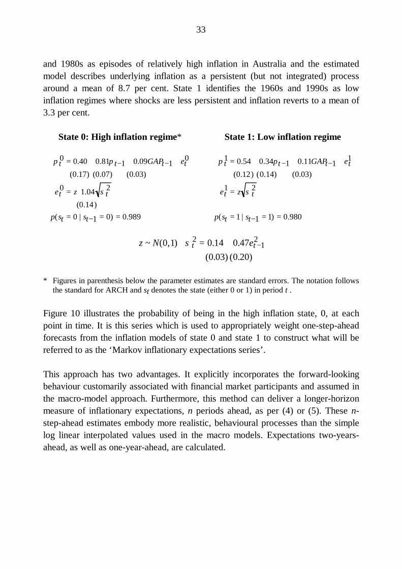
and 1980s as episodes of relatively high inflation in Australia and the estimatedmodel describes underlying inflation as a persistent (but not integrated) processaround a mean of 8.7 per cent. State 1 identifies the 1960s and 1990s as lowinflation regimes where shocks are less persistent and inflation reverts to a mean of3.3 per cent.
State 0: High inflation regime* State 1: Low inflation regime
πt0 = 0.40 + 0.81πt− 1 + 0.09GAPt− 1 + εt
0
(0.17) (0.07) (0.03)
εt0 = z⋅1.04 σt
2
(0.14)p(st = 0 | st− 1 = 0) = 0.989
πt1 = 0.54 + 0.34πt − 1 + 0.11GAPt− 1 + εt
1
(0.12) (0.14) (0.03)
εt1 = z σt
2
p(st = 1 | st− 1 = 1) = 0.980
z ~ N(0,1) σt2 = 0.14 + 0.47εt − 1
2
(0.03) (0.20)
* Figures in parenthesis below the parameter estimates are standard errors. The notation followsthe standard for ARCH and st denotes the state (either 0 or 1) in period t .
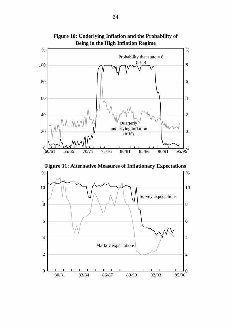
Figure 10 illustrates the probability of being in the high inflation state, 0, at eachpoint in time. It is this series which is used to appropriately weight one-step-aheadforecasts from the inflation models of state 0 and state 1 to construct what will bereferred to as the ‘Markov inflationary expectations series’.
This approach has two advantages. It explicitly incorporates the forward-lookingbehaviour customarily associated with financial market participants and assumed inthe macro-model approach. Furthermore, this method can deliver a longer-horizonmeasure of inflationary expectations, n periods ahead, as per (4) or (5). These n-step-ahead estimates embody more realistic, behavioural processes than the simplelog linear interpolated values used in the macro models. Expectations two-years-ahead, as well as one-year-ahead, are calculated.
34
Figure 10: Underlying Inflation and the Probability ofBeing in the High Inflation Regime
0
20
40
60
80
100
-2
0
2
4
6
8
Quarterlyunderlying inflation
(RHS)
Probability that state = 0(LHS)
%
95/9690/9185/8680/8175/7670/7165/66
%
60/61
Figure 11: Alternative Measures of Inflationary Expectations
0
2
4
6
8
10
0
2
4
6
8
10
Survey expectations
95/9692/9389/9086/8783/8480/81
% %
Markov expectations
35
It is clear from Figure 11 that the behaviour of the Markov expectations series isquite distinct from that of the consumer survey measure. For exposition, only theMarkov one-year-ahead inflationary expectations, generated by agents with perfectforesight of the output gap, EPFt (πt + 4 ) , are illustrated in Figure 11. Thealternative, mean-reverting output gap specification and the two-year-aheadforecasts of Markov expectations exhibit similar patterns and timing.
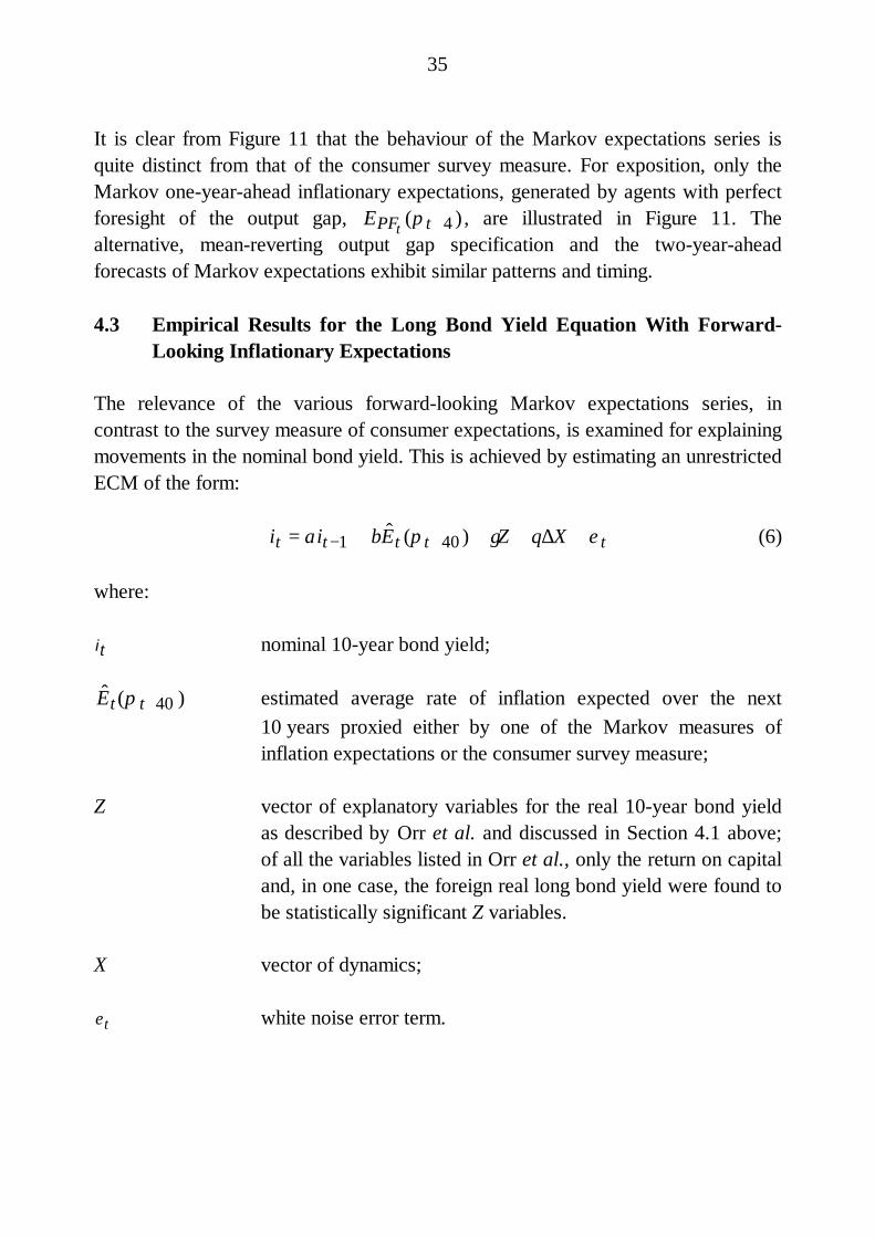
4.3 Empirical Results for the Long Bond Yield Equation With Forward-Looking Inflationary Expectations
The relevance of the various forward-looking Markov expectations series, incontrast to the survey measure of consumer expectations, is examined for explainingmovements in the nominal bond yield. This is achieved by estimating an unrestrictedECM of the form:
it = αit − 1 + β E t (πt + 40 ) + γZ + θ∆X + εt (6)
where:
i t nominal 10-year bond yield;
E t (π t+ 40 ) estimated average rate of inflation expected over the next10 years proxied either by one of the Markov measures ofinflation expectations or the consumer survey measure;
Z vector of explanatory variables for the real 10-year bond yieldas described by Orr et al. and discussed in Section 4.1 above;of all the variables listed in Orr et al., only the return on capitaland, in one case, the foreign real long bond yield were found tobe statistically significant Z variables.
X vector of dynamics;
εt white noise error term.
36
Four lags of each of the differenced explanatory variables were initially included inthe dynamic specification of the model; F-tests were then used to derive theparsimonious final model. Table 4 summarises the results from estimation of (6)using the competing measures of E t (π t+ 40 ) .
Table 4: Australian Nominal Long Bond Yield EquationDependent variable: ∆i
(1981:Q1-1995:Q2)
t Ε (πt+ n) Z
ModelNo.
Measure of
t Ε ( t + 40π )ß
(t-statistic)α
Speed ofadjustment
(t-stat)
γοReturn on
capital(t-stat)
γ1r*
(t-stat)
R 2 H0 : α = − β(p-value)
1 ΕPFt (πt+ 4) 0.204(4.80)
-0.241(4.36)
0.079(2.68)
0.13(1.90)
0.332 0.61
2 ΕMRt (πt + 4) 0.223(4.10)
-0.226(4.38)
0.083(2.97)
— 0.284 0.93
3 Survey 0.262(3.09)
-0.299(3.47)
0.083(2.31)
— 0.271 0.33
4 ΕPFt (π t+ 8 ) 0.091(2.05)
-0.065(2.95)
— — 0.216 0.32
5 ΕMRt (π t+ 8 ) 0.245(3.21)
-0.210(3.61)
0.066(2.33)
— 0.214 0.44
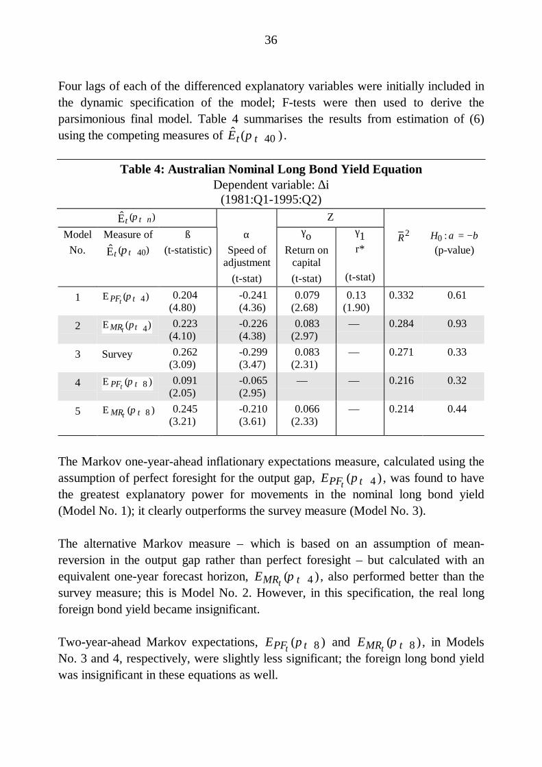
The Markov one-year-ahead inflationary expectations measure, calculated using theassumption of perfect foresight for the output gap, EPFt (πt + 4 ) , was found to havethe greatest explanatory power for movements in the nominal long bond yield(Model No. 1); it clearly outperforms the survey measure (Model No. 3).
The alternative Markov measure – which is based on an assumption of mean-reversion in the output gap rather than perfect foresight – but calculated with anequivalent one-year forecast horizon, EMRt (π t+ 4 ) , also performed better than thesurvey measure; this is Model No. 2. However, in this specification, the real longforeign bond yield became insignificant.
Two-year-ahead Markov expectations, EPFt (πt + 8 ) and EMRt (π t+ 8 ) , in ModelsNo. 3 and 4, respectively, were slightly less significant; the foreign long bond yieldwas insignificant in these equations as well.
37
The remainder of this section concentrates on the results obtained from Model No.1’s specification (see Table C.3 in Appendix C for the full estimated dynamics):
∆it = αit− 1 + β EPFt (πt+ 4 )[ ]t− 1+ γ0 Re tCapt− 1 + γ1rt− 1
* +
θ0 ii=0
2∑ ∆rt − i + θ1∆ ΕPFt
(π t+ 4 )[ ]t − 1+ θ2 gt− 3 + εt
(7)
where:
it nominal Australian 10-year bond yield;
ΕPFt (πt+ 4 ) Markov model estimates of inflationary expectations asdefined in (4) above or consumer survey measure;
RetCap return on capital;
r* US real 10-year bond rate;
g domestic GDP growth;
εt white noise error term;
∆ difference operator.
Full-sample predictions from this very simple nominal long bond yield equation fitthe actual data very well (Figure 12).

38
Figure 12: Nominal 10-year Bond Yield Dynamic Simulationand Out-of-Sample Forecasts
8
10
12
14
16
8
10
12
14
16
6
8
10
12
14
16
6
8
10
12
14
16
95/9692/9389/9086/8783/84
Predicted
Actual
Predicted
Actual
Dynamicforecast
% %
%%
80/81
Dynamic forecasts
As in Section 4.1, out-of-sample forecasts were obtained by estimating the model toDecember 1991; actual values of the exogeneous variables were then used toforecast the nominal long bond yield forward in time. The model anticipates theturning point in bond yields in late 1993 as well as their subsequent pick-up over1994, presumably because it contains the foreign bond yield (r*); the other modelsdid not.
The null hypothesis in the final column of Table 4 tests that the Fisher Hypothesisholds, such that movements in inflationary expectations are matched one-for-one bymovements in the nominal interest rate. This restriction is necessary for validreparameterisation of Model No. 1 (equation (7)) as a real bond yield equation; thenull hypothesis could not be rejected. Trivially, additional restrictions are also
39
accepted such that this model, re-estimated as a real bond yield equation, deliversthe same parameter estimates on the Z variables.
In this way, while equation (3) in Section 4.1, presented a model of the real10-year bond yield, deflated with backward-looking expectations, equation (7)provides an alternative model wherein real yields are constructed using a forward-looking Markov measure of expectations. The main features of this latter model arelisted below.
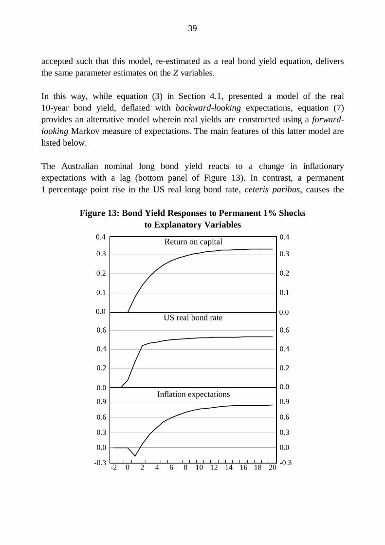
The Australian nominal long bond yield reacts to a change in inflationaryexpectations with a lag (bottom panel of Figure 13). In contrast, a permanent1 percentage point rise in the US real long bond rate, ceteris paribus, causes the
Figure 13: Bond Yield Responses to Permanent 1% Shocksto Explanatory Variables
0.1
0.2
0.3
0.1
0.2
0.3
0.2
0.4
0.6
0.2
0.4
0.6
-0.3
0.0
0.3
0.6
0.9
-0.3
0.0
0.3
0.6
0.9
Return on capital
US real bond rate
Inflation expectations
20181614121086420-2
0.4
0.00.0
0.00.0
0.4
40
Australian real long bond yield to react instantaneously; by the second quarter afterthe shock, the domestic long bond yield would be around 0.54 of a percentage pointhigher (panel 2, Figure 13; this is larger than the 0.30 of a percentage point impliedby the Orr et al. cross-section estimates for Australia).
Consistent with the result obtained from estimation of equation (3), a permanent1 percentage point improvement in the return on Australian capital raises thedomestic real yield by around 1
3 of a percentage point; this response occurs moreslowly than that estimated for a change in the US real rate (panel 1, Figure 13).
5. Conclusion
There is no single, simple conclusion to be drawn from this research, but, rather, aseries of points can be made.
Interest rates and exchange rates now form part of the transmission mechanism bywhich policy changes feed through to the broader economy. Expectations play acritical role in this mechanism, affecting both the timing and speed of transmission.Theoretical discussions of interest and exchange rate markets typically characteriseexpectations as forward looking. However, it has been difficult to model this type ofbehaviour within an empirical framework.
One approach has been to rely on the relevant components of full-scale,intertemporal macroeconomic models. These models typically embody theoreticallyconsistent, long-run properties and rational, forward-looking expectations in thefinancial sector. In Australian macroeconomic models, such exchange rate and bondyield equations are not estimated; they reflect orthodox theoretical considerationsincluding uncovered interest parity and the term-structure hypothesis. But thetextbook-style results produced by these macro models have limited relevance forpractical policymaking.
Alternatively, single-equation, behavioural models can be used to document theobserved historical relationships in the data. These have typically assumed thatexpectations are formed adaptively, that is, are backward looking. The research inthis paper concentrates on introducing forward-looking, policy elements intobehavioural models of the Australian real exchange rate and long bond yield.
41
Given that expectations play a central role in determining the responses to variousshocks, the macroeconomic and behavioural model approaches are probably bestdistinguished by a comparison of impulse response functions. In particular, thesetwo methodologies provide different characterisations of the behaviour of the realexchange rate. In the macro-model framework, monetary policy shocks elicit aninstantaneous change in the real exchange rate which is subsequently and graduallyunwound. In contrast, the behavioural model developed in this paper does not returnthis instantaneous ‘jump’ response. Instead, the real exchange rate only graduallytransmits a change in monetary policy through to the broader economy so that thefull impact of the policy change through this channel is felt with a lag. Despite verydifferent adjustment paths, both models produce final responses of a similar order ofmagnitude.
On the other hand, about half of a sustained terms of trade shock is finally passedthrough to the real exchange rate in the macro models; this occurs through an initialjump in the exchange rate, followed by gradual adjustment towards the long run.While this result is theoretically appealing, it does not describe the actual behaviourof the Australian real exchange rate. The behavioural model estimates that the realexchange rate moves much more closely with terms of trade shocks, regardless ofwhether the shocks are temporary or sustained over very long periods. Someovershooting is estimated to occur immediately. This result is puzzling, but it isconsistent with the idea that agents in the foreign exchange market look forwardover only a relatively short horizon. The inherent difficulty of incorporatinginefficient mechanisms into the macro-model framework may be one source of thedisparity between the macro-model results and those recorded by the behaviouralmodels.
Incorporating forward-looking behaviour into a bond yield equation is lessstraightforward. In this paper, it is achieved by explicitly modelling the formation ofinflation expectations. Expectations are generated from a series of assessmentsabout the probability of shifting between a high and a low inflation regime. This isparticularly apt in Australia, since a discrete shift in inflationary expectationsoccurred in the early 1990s. The superior performance of the shorter-horizonmeasures of inflation expectations suggests that some myopia may exist in thismarket as well. Further work in this area might consider whether there are roles forboth forward and backward-looking elements within the long bond rate model.

42
Appendix A: Data Sources
The data for Section 3 of the paper were collected for the period fromSeptember 1973 to June 1995. The data for Section 4 were collected for the periodfrom December 1979 to June 1995. All indexes are based to 1989/90 = 100. ThisAppendix lists each of the variables used in the paper together with their method ofconstruction and original data source(s).
Real exchange rateIndex.Reserve Bank of Australia.
Terms of tradeIndex; Seasonally adjusted; Goods and services measure.The terms of trade was spliced to the goods and services trend measure atSeptember 1974.Australian Bureau of Statistics, Cat. No. 5302.0, Table 9.
Nominal Gross Domestic Product (GDP)$m; Seasonally adjusted; Income measure.Australian Bureau of Statistics, Cat. No. 5206.0.
Real Gross Domestic ProductAverage measure; The growth variable is the quarterly growth of real GDP.Australian Bureau of Statistics, Cat. No. 5206.0.
Cumulated current accountCurrent account balance; $m; Seasonally adjusted.The cumulated current account for each quarter is calculated as the cumulative sumof quarterly current account balances from September 1959 and taken as aproportion of annualised GDP:
ieΣ j=1t current account j / GDPt ×4( )( )
Australian Bureau of Statistics, Cat. No. 5302.0, Table 3.

43
Net foreign liabilitiesNet International Investment Position at end of period.$m.Annual data for the period June 1974 – June 1985, quarterly data thereafter.Expressed as a proportion of annual GDP.June 1974-June 1978: Reserve Bank of Australia Occasional Paper No. 8.June 1979-June 1995: Australian Bureau of Statistics, Cat. No. 5306.0, Table 1.
FiscalCommonwealth Government Budget Balance;The fiscal variable for the four quarters of each fiscal year is measured as thechange in the annual Commonwealth Government Budget Balance as a proportionof GDP, calculated on a quarterly basis.1995/96 Commonwealth Budget Paper No. 1.
Cash rateReserve Bank of Australia Bulletin, Table F.1, and internal sources.
90-day bank billReserve Bank of Australia Bulletin, Table F.1, and internal sources.
10-year bond rateReserve Bank of Australia Bulletin, Table F.2, and internal sources.
GDP in US dollarsAnnual GDP for United States, Canada and the United Kingdom, measured inmillions of US dollars, are applied as weights in the construction of world variables.The UK measure of GDP is quarterly and is converted into an annual measure.
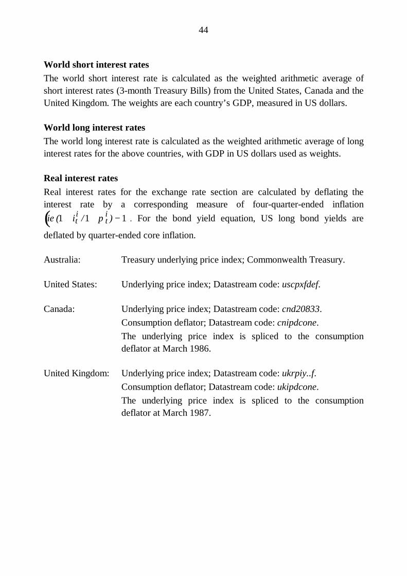
44
World short interest ratesThe world short interest rate is calculated as the weighted arithmetic average ofshort interest rates (3-month Treasury Bills) from the United States, Canada and theUnited Kingdom. The weights are each country’s GDP, measured in US dollars.
World long interest ratesThe world long interest rate is calculated as the weighted arithmetic average of longinterest rates for the above countries, with GDP in US dollars used as weights.
Real interest ratesReal interest rates for the exchange rate section are calculated by deflating theinterest rate by a corresponding measure of four-quarter-ended inflationie (1 + it
i /1 + π ti ) − 1( ). For the bond yield equation, US long bond yields are
deflated by quarter-ended core inflation.
Australia: Treasury underlying price index; Commonwealth Treasury.
United States: Underlying price index; Datastream code: uscpxfdef.
Canada: Underlying price index; Datastream code: cnd20833.Consumption deflator; Datastream code: cnipdcone.The underlying price index is spliced to the consumptiondeflator at March 1986.
United Kingdom: Underlying price index; Datastream code: ukrpiy..f.Consumption deflator; Datastream code: ukipdcone.The underlying price index is spliced to the consumptiondeflator at March 1987.
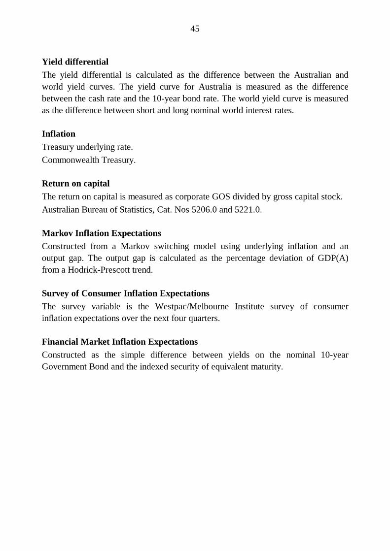
45
Yield differentialThe yield differential is calculated as the difference between the Australian andworld yield curves. The yield curve for Australia is measured as the differencebetween the cash rate and the 10-year bond rate. The world yield curve is measuredas the difference between short and long nominal world interest rates.
InflationTreasury underlying rate.Commonwealth Treasury.
Return on capitalThe return on capital is measured as corporate GOS divided by gross capital stock.Australian Bureau of Statistics, Cat. Nos 5206.0 and 5221.0.
Markov Inflation ExpectationsConstructed from a Markov switching model using underlying inflation and anoutput gap. The output gap is calculated as the percentage deviation of GDP(A)from a Hodrick-Prescott trend.
Survey of Consumer Inflation ExpectationsThe survey variable is the Westpac/Melbourne Institute survey of consumerinflation expectations over the next four quarters.
Financial Market Inflation ExpectationsConstructed as the simple difference between yields on the nominal 10-yearGovernment Bond and the indexed security of equivalent maturity.
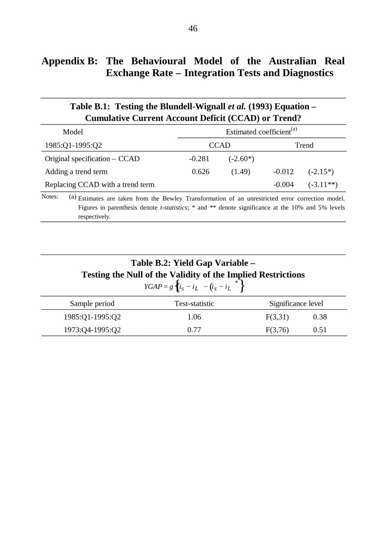
46
Appendix B: The Behavioural Model of the Australian RealExchange Rate – Integration Tests and Diagnostics
Table B.1: Testing the Blundell-Wignall et al. (1993) Equation –Cumulative Current Account Deficit (CCAD) or Trend?
Model Estimated coefficient(a)
1985:Q1-1995:Q2 CCAD Trend
Original specification – CCAD -0.281 (-2.60*)
Adding a trend term 0.626 (1.49) -0.012 (-2.15*)
Replacing CCAD with a trend term -0.004 (-3.11**)Notes: (a) Estimates are taken from the Bewley Transformation of an unrestricted error correction model.
Figures in parenthesis denote t-statistics; * and ** denote significance at the 10% and 5% levelsrespectively.
Table B.2: Yield Gap Variable –Testing the Null of the Validity of the Implied Restrictions
YGAP = γ is − iL( )− is − iL( )*{ }Sample period Test-statistic Significance level
1985:Q1-1995:Q2 1.06 F(3,31) 0.38
1973:Q4-1995:Q2 0.77 F(3,76) 0.51
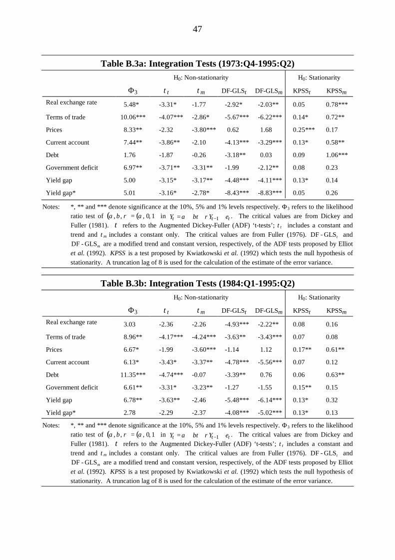
47
Table B.3a: Integration Tests (1973:Q4-1995:Q2)H0: Non-stationarity H0: Stationarity
Φ 3 ττ τµ DF-GLSτ DF-GLSµ KPSSτ KPSSµReal exchange rate 5.48* -3.31* -1.77 -2.92* -2.03** 0.05 0.78***
Terms of trade 10.06*** -4.07*** -2.86* -5.67*** -6.22*** 0.14* 0.72**
Prices 8.33** -2.32 -3.80*** 0.62 1.68 0.25*** 0.17
Current account 7.44** -3.86** -2.10 -4.13*** -3.29*** 0.13* 0.58**
Debt 1.76 -1.87 -0.26 -3.18** 0.03 0.09 1.06***
Government deficit 6.97** -3.71** -3.31** -1.99 -2.12** 0.08 0.23
Yield gap 5.00 -3.15* -3.17** -4.48*** -4.11*** 0.13* 0.14
Yield gap* 5.01 -3.16* -2.78* -8.43*** -8.83*** 0.05 0.26
Notes: *, ** and *** denote significance at the 10%, 5% and 1% levels respectively. Φ 3 refers to the likelihoodratio test of α , β, ρ( )= α , 0, 1( ) in Yt =α + βt + ρYt − 1 + et . The critical values are from Dickey andFuller (1981). τ refers to the Augmented Dickey-Fuller (ADF) ‘t-tests’; ττ includes a constant andtrend and τµ includes a constant only. The critical values are from Fuller (1976). DF - GLSτ andDF - GLSµ are a modified trend and constant version, respectively, of the ADF tests proposed by Elliotet al. (1992). KPSS is a test proposed by Kwiatkowski et al. (1992) which tests the null hypothesis ofstationarity. A truncation lag of 8 is used for the calculation of the estimate of the error variance.
Table B.3b: Integration Tests (1984:Q1-1995:Q2)H0: Non-stationarity H0: Stationarity
Φ 3 ττ τµ DF-GLSτ DF-GLSµ KPSSτ KPSSµReal exchange rate 3.03 -2.36 -2.26 -4.93*** -2.22** 0.08 0.16
Terms of trade 8.96** -4.17*** -4.24*** -3.63** -3.43*** 0.07 0.08
Prices 6.67* -1.99 -3.60*** -1.14 1.12 0.17** 0.61**
Current account 6.13* -3.43* -3.37** -4.78*** -5.56*** 0.07 0.12
Debt 11.35*** -4.74*** -0.07 -3.39** 0.76 0.06 0.63**
Government deficit 6.61** -3.31* -3.23** -1.27 -1.55 0.15** 0.15
Yield gap 6.78** -3.63** -2.46 -5.48*** -6.14*** 0.13* 0.32
Yield gap* 2.78 -2.29 -2.37 -4.08*** -5.02*** 0.13* 0.13
Notes: *, ** and *** denote significance at the 10%, 5% and 1% levels respectively. Φ 3 refers to the likelihoodratio test of α , β, ρ( )= α , 0, 1( ) in Yt =α + βt + ρYt − 1 + et . The critical values are from Dickey andFuller (1981). τ refers to the Augmented Dickey-Fuller (ADF) ‘t-tests’; ττ includes a constant andtrend and τµ includes a constant only. The critical values are from Fuller (1976). DF - GLSτ andDF - GLSµ are a modified trend and constant version, respectively, of the ADF tests proposed by Elliotet al. (1992). KPSS is a test proposed by Kwiatkowski et al. (1992) which tests the null hypothesis ofstationarity. A truncation lag of 8 is used for the calculation of the estimate of the error variance.
48
The DF-GLS test (Elliot et al. 1992) is a modified version of the AugmentedDickey-Fuller (ADF) t-test, having the advantages that it exhibits superior powerproperties and suffers from only small size distortions in finite samples. The testingprocedure involves firstly demeaning or detrending the series using GeneralisedLeast Squares and then running the ADF test regression using that series. Theconstant and time trend terms are omitted from the test regression. The t-statistic on(ρ-1) is then used to test for significance against the appropriate critical value. Thedemeaned case (DF-GLS
µ) is comparable to including a constant term in the ADF
test; the critical values are taken from Fuller (1976) and the no-constant variant ofthe MacKinnon (1991) table. The detrended case (DF-GLSτ) is comparable toincluding a constant and a time trend in the ADF test; the critical values have beentabulated by Elliot et al.
The KPSS (1992) test is applied in the following way. All series can be written asthe sum of a trend (ξt), a random walk (rt), and a stationary component (εt) suchthat:
yt = ξt + rt + εtwhere: rt=rt-1+ut.
If the series is stationary (that is, there is no random walk component), the varianceof ut will be zero. The test statistic for the null hypothesis of no unit root is an LMstatistic which is a function of estimated residuals and an estimate of the long-runerror variance. These residuals are either the demeaned series (ηµ ) or the demeanedand detrended series (ητ ). The critical values for these tests are detailed inKwiatkowski et al. (1992, p.166).
These tests provide evidence over the full sample period (1973:Q4-1995:Q2) thatthe real exchange rate; terms of trade; interest differentials; yield gaps; currentaccount deficit; government budget balance; and relative productivity differentialsare I(0), with the first two series exhibiting this stationarity around a trend. Theseconclusions are also supportable over the shorter sample period (1984:Q1-1995:Q2).
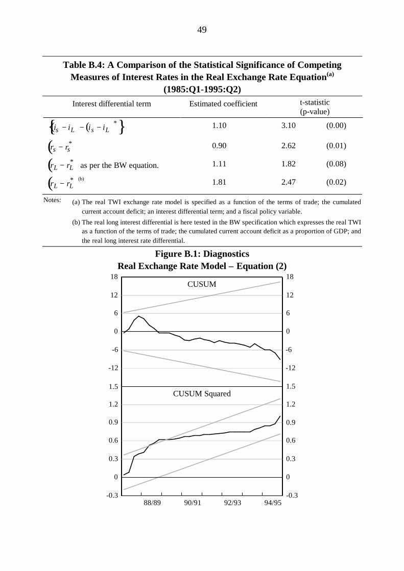
49
Table B.4: A Comparison of the Statistical Significance of CompetingMeasures of Interest Rates in the Real Exchange Rate Equation(a)
(1985:Q1-1995:Q2)Interest differential term Estimated coefficient t-statistic
(p-value)
is − iL( )− is − iL( )*{ } 1.10 3.10 (0.00)
rs − rs*( ) 0.90 2.62 (0.01)
rL − rL*( ) as per the BW equation. 1.11 1.82 (0.08)
rL − rL*( )(b) 1.81 2.47 (0.02)
Notes: (a) The real TWI exchange rate model is specified as a function of the terms of trade; the cumulatedcurrent account deficit; an interest differential term; and a fiscal policy variable.
(b) The real long interest differential is here tested in the BW specification which expresses the real TWIas a function of the terms of trade; the cumulated current account deficit as a proportion of GDP; andthe real long interest rate differential.
Figure B.1: DiagnosticsReal Exchange Rate Model – Equation (2)
-12
-6
0
6
12
18
-12
-6
0
6
12
18
88/89 90/91 92/93 94/95-0.3
0
0.3
0.6
0.9
1.2
-0.3
0
0.3
0.6
0.9
1.2
1.5
CUSUM
CUSUM Squared1.5
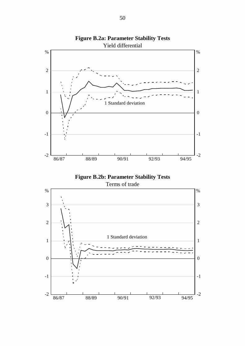
50
Figure B.2a: Parameter Stability TestsYield differential
-2
-1
0
1
2
-2
-1
0
1
2
94/9592/9390/9188/8986/87
%%
1 Standard deviation
Figure B.2b: Parameter Stability TestsTerms of trade
-2
-1
0
1
2
3
-2
-1
0
1
2
3
1 Standard deviation
94/9592/9390/9188/8986/87
%%
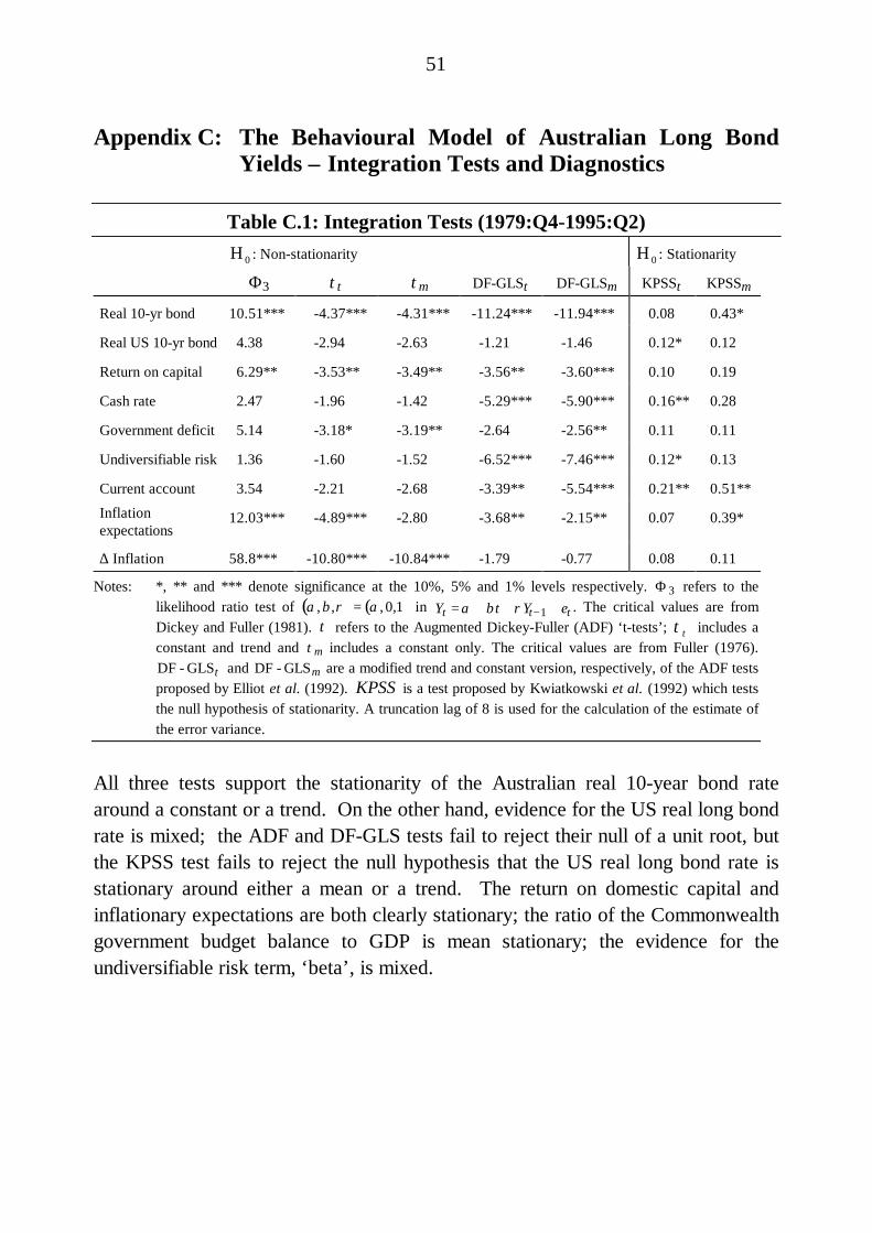
51
Appendix C: The Behavioural Model of Australian Long BondYields – Integration Tests and Diagnostics
Table C.1: Integration Tests (1979:Q4-1995:Q2)H 0 : Non-stationarity H 0 : Stationarity
Φ 3 ττ τµ DF-GLSτ DF-GLSµ KPSSτ KPSSµ
Real 10-yr bond 10.51*** -4.37*** -4.31*** -11.24*** -11.94*** 0.08 0.43*
Real US 10-yr bond 4.38 -2.94 -2.63 -1.21 -1.46 0.12* 0.12
Return on capital 6.29** -3.53** -3.49** -3.56** -3.60*** 0.10 0.19
Cash rate 2.47 -1.96 -1.42 -5.29*** -5.90*** 0.16** 0.28
Government deficit 5.14 -3.18* -3.19** -2.64 -2.56** 0.11 0.11
Undiversifiable risk 1.36 -1.60 -1.52 -6.52*** -7.46*** 0.12* 0.13
Current account 3.54 -2.21 -2.68 -3.39** -5.54*** 0.21** 0.51**
Inflationexpectations
12.03*** -4.89*** -2.80 -3.68** -2.15** 0.07 0.39*
∆ Inflation 58.8*** -10.80*** -10.84*** -1.79 -0.77 0.08 0.11
Notes: *, ** and *** denote significance at the 10%, 5% and 1% levels respectively. Φ 3 refers to thelikelihood ratio test of α ,β,ρ( )= α , 0,1( ) in Yt =α + βt + ρYt − 1 + et . The critical values are fromDickey and Fuller (1981). τ refers to the Augmented Dickey-Fuller (ADF) ‘t-tests’; ττ includes aconstant and trend and τµ includes a constant only. The critical values are from Fuller (1976).DF - GLSτ and DF - GLSµ are a modified trend and constant version, respectively, of the ADF testsproposed by Elliot et al. (1992). KPSS is a test proposed by Kwiatkowski et al. (1992) which teststhe null hypothesis of stationarity. A truncation lag of 8 is used for the calculation of the estimate ofthe error variance.
All three tests support the stationarity of the Australian real 10-year bond ratearound a constant or a trend. On the other hand, evidence for the US real long bondrate is mixed; the ADF and DF-GLS tests fail to reject their null of a unit root, butthe KPSS test fails to reject the null hypothesis that the US real long bond rate isstationary around either a mean or a trend. The return on domestic capital andinflationary expectations are both clearly stationary; the ratio of the Commonwealthgovernment budget balance to GDP is mean stationary; the evidence for theundiversifiable risk term, ‘beta’, is mixed.
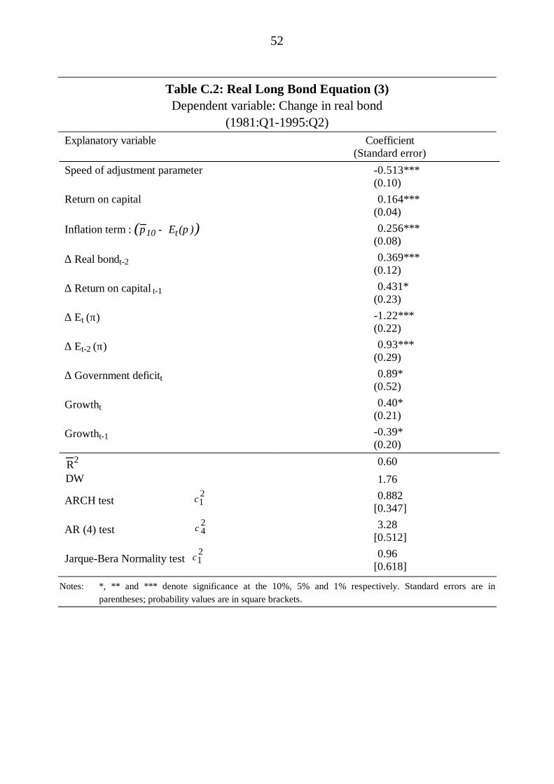
52
Table C.2: Real Long Bond Equation (3)Dependent variable: Change in real bond
(1981:Q1-1995:Q2)Explanatory variable Coefficient
(Standard error)Speed of adjustment parameter -0.513***
(0.10)Return on capital 0.164***
(0.04)Inflation term : π 10 − Et (π)( ) 0.256***
(0.08)
∆ Real bondt-2 0.369***(0.12)
∆ Return on capital t-1 0.431*(0.23)
∆ Εt (π) -1.22***(0.22)
∆ Εt-2 (π) 0.93***(0.29)
∆ Government deficitt 0.89*(0.52)
Growtht 0.40*(0.21)
Growtht-1 -0.39*(0.20)
R 2 0.60DW 1.76
ARCH test χ12 0.882
[0.347]
AR (4) test χ42 3.28
[0.512]
Jarque-Bera Normality test χ12 0.96
[0.618]
Notes: *, ** and *** denote significance at the 10%, 5% and 1% respectively. Standard errors are inparentheses; probability values are in square brackets.
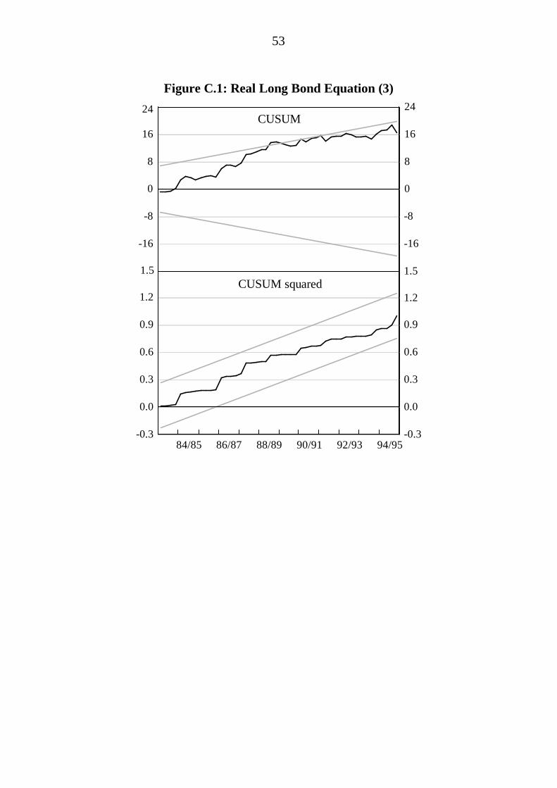
53
Figure C.1: Real Long Bond Equation (3)
-16
-8
0
8
16
-16
-8
0
8
16
24CUSUM
84/85 86/87 88/89 90/91 92/93 94/95-0.3
0.0
0.3
0.6
0.9
1.2
-0.3
0.0
0.3
0.6
0.9
1.2
1.5CUSUM squared
24
1.5
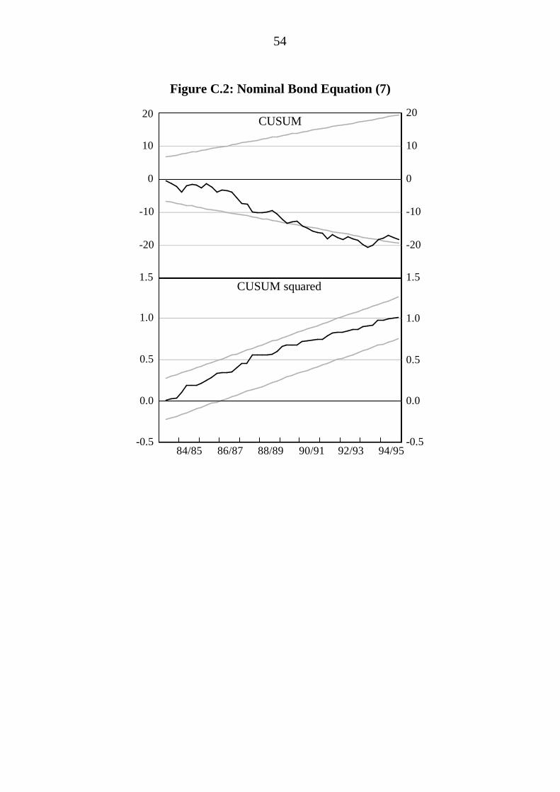
54
Figure C.2: Nominal Bond Equation (7)
-20
-10
0
10
-20
-10
0
10
20
-0.5
0.0
0.5
1.0
-0.5
0.0
0.5
1.0
1.5
CUSUM
CUSUM squared
94/9592/9390/9188/8986/8784/85
20
1.5
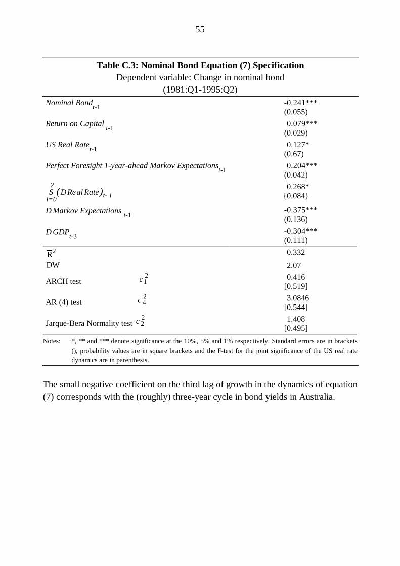
55
Table C.3: Nominal Bond Equation (7) SpecificationDependent variable: Change in nominal bond
(1981:Q1-1995:Q2)Nominal Bondt-1 -0.241***
(0.055)Return on Capital t-1 0.079***
(0.029)US Real Ratet-1 0.127*
(0.67)Perfect Foresight 1-year-ahead Markov Expectationst-1 0.204***
(0.042)
Σi= 0
2∆ Real Rate( )t− i
0.268*{0.084}
∆ Markov Expectations t-1 -0.375***(0.136)
∆ GDPt-3-0.304***(0.111)
R 2 0.332DW 2.07
ARCH test χ12 0.416
[0.519]
AR (4) test χ42 3.0846
[0.544]
Jarque-Bera Normality test χ22 1.408
[0.495]Notes: *, ** and *** denote significance at the 10%, 5% and 1% respectively. Standard errors are in brackets
(), probability values are in square brackets and the F-test for the joint significance of the US real ratedynamics are in parenthesis.
The small negative coefficient on the third lag of growth in the dynamics of equation(7) corresponds with the (roughly) three-year cycle in bond yields in Australia.
56
REFERENCES
Amano, R. and S. van Norden (1992), ‘A Forecasting Equation for the Canada-U.S. Dollar Exchange Rate’, The Exchange Rate and the Economy, Proceedings ofa conference held at the Bank of Canada, 22-23 June, pp. 207-265.
Bayoumi, T., P. Clark, S. Symansky and M. Taylor (1994), ‘The Robustness ofEquilibrium Exchange Rate Calculations to Alternative Assumptions andMethodologies’, in J. Williamson (ed.), Estimating Equilibrium Exchange Rates,Institute for International Economics, Washington, DC.
Bleaney, M. (1993), ‘The Australian Real Exchange Rate, Terms of Trade andPrimary Commodity Prices 1901-91’, Credit Research Paper No. 93/6, Universityof Nottingham.
Blundell-Wignall, A. and M. Thomas (1987), ‘Deviations from Purchasing PowerParity: The Australian Case’, Reserve Bank of Australia Research DiscussionPaper No. 8711.
Blundell-Wignall, A., J. Fahrer and A. Heath (1993), ‘Major Influences on theAustralian Dollar Exchange Rate’, in A. Blundell-Wignall (ed.), The ExchangeRate, International Trade and the Balance of Payments, Proceedings of aConference, Reserve Bank of Australia, pp. 30-78.
Clark, P., L. Bartolini, T. Bayoumi and S. Symansky (1994), ‘Exchange Ratesand Economic Fundamentals: A Framework for Analysis’, IMF Occasional Paper,December.
Cook, T. and T. Hahn (1990), ‘Interest Rate Expectations and the Slope of theMoney Market Yield Curve’, Federal Reserve Bank of Richmond EconomicReview, 76(5), pp. 3-26.
De Kock, G. and T. Deleire (1994), ‘The Role of the Exchange Rate in theMonetary Transmission Mechanism: A Time-Series Analysis’, Federal ReserveBank of New York, Research Paper No. 9412.
57
Dickey, D.A. and W.A. Fuller (1981), ‘Likelihood Ratio Statistics forAutoregressive Time Series with a Unit Root’, Econometrica, 49(4),pp. 1057-1072.
Downes, P. (1995), ‘An Introduction to the TRYM Model: Applications andLimitations’, 1995 IFAC Symposium on Modelling and Control of National andRegional Economies Conference Volume, 2-5th July, The Institution of Engineers,Australia.
Dwyer, J., C. Kent and A. Pease (1994), ‘Exchange Rate Pass-Through: Testingthe Small Country Assumption for Australia’, Economic Record, 70(211), pp. 408-423.
Edey, M. (1990), ‘Operating Objectives for Monetary Policy’, Reserve Bank ofAustralia Research Discussion Paper No. 9007.
Edey, M. and J. Romalis (1996), ‘Issues in Modelling Monetary Policy’, ReserveBank of Australia Research Discussion Paper No. 9604.
Elliot, G., T.J. Rothenberg and J.H. Stock (1992), ‘Efficient Tests for anAutoregressive Unit Root’, Mimeo, November.
Estrella, A. and F.S. Mishkin (1995), ‘The Term Structure of Interest Rates andIts Role in Monetary Policy for the European Central Bank’, NBER Working PaperNo.5279.
Evans, M. and P. Wachtel (1993), ‘Inflation Regimes and the Sources of InflationUncertainty’, Journal of Money, Credit and Banking, 25(3), pp. 475-511.
Fuller, W.A. (1976), Introduction to Statistical Time Series, Wiley, New York.
Goodhart, C. (1988), ‘The Foreign Exchange Market: A Random Walk with aDragging Anchor’, Economica, 55, November, pp. 437-460.
Goodwin, T.H. (1993), ‘Business-Cycle Analysis with a Markov-SwitchingModel’, Journal of Business and Economic Statistics, 11(3), pp. 331-339.
58
Gruen, D.W.R. and J. Wilkinson (1991), ‘Australia’s Real Exchange Rate – Is itExplained by the Terms of Trade or by Real Interest Differentials?’, Reserve Bankof Australia Research Discussion Paper No. 9108.
Gruen, D.W.R. and T. Kortian (1996), ‘Why does the Australian Dollar Movewith the Terms of Trade?’, Reserve Bank of Australia Research Discussion PaperNo. 9601.
Hamilton, J.D. (1989), ‘A New Approach to the Economic Analysis ofNon-Stationary Time Series and the Business Cycle’, Econometrica, 57(2),pp. 357-384.
Hamilton, J.D. (1990), ‘Analysis of Time Series Subject to Changes in Regime’,Journal of Econometrics, 45, pp. 39-70.
Hodrick, R.J. (1987), ‘The Empirical Evidence on the Efficiency of Forward andFutures Foreign Exchange Markets’, Fundamentals of Pure and AppliedEconomics, 24, Harwood Academic Publishers, New York.
Huizinga, J. (1987), ‘An Empirical Investigation of the Long-Run Behaviour ofReal Exchange Rates’, Carnegie-Rochester Conference Series on Public Policy,27, pp. 149-214.
In’t Veld, J.W. (1991), ‘Fundamental Balance and Equilibrium Exchange Rates’,Journal of International Money and Finance, 10(2), pp. 279-291.
Isard, P. (1983), ‘An Accounting Framework and Some Issues for Modelling HowExchange Rates Respond to the News’, in J. Frenkel (ed.), Exchange Rates andInternational Macroeconomics, University of Chicago Press, Chicago.
Isard, P. (1988), ‘Exchange Rate Modelling: An Assessment of AlternativeApproaches’, in R.C. Bryant et al. (eds), Empirical Macroeconomics forInterdependent Economies, The Brookings Institute, Washington, D.C.,pp. 183-201.
Kmenta, J. (1990), Elements of Econometrics (Second Edition), MaxwellMacmillan, New York.
59
Kwiatkowski, D., P.C.B. Phillips, P. Schmidt and Y. Shin (1992), ‘Testing theNull Hypothesis of Stationary Against the Alternative of a Unit Root’, Journal ofEconometrics, 54, pp. 159-178.
Laxton, D., N. Ricketts and D. Rose (1994), ‘Uncertainty, Learning and PolicyCredibility’, Economic Behaviour and Policy Choice Under Price Stability,Proceedings of a Conference Held at the Bank of Canada, Ottawa, pp. 173-234.
Liu, C.Y. and J. He (1991), ‘Do Real Exchange Rates Follow Random Walks? AHeteroscedasticity-Robust Autocorrelation Test’, International Economic Journal,5(3), pp. 39-48.
Lowe, P. (1994), ‘The Link Between the Cash Rate and Market Interest Rates,Reserve Bank of Australia Research Discussion Paper No. 9504.
MacKinnon, J.G. (1991), ‘Critical Values for Cointegration Tests’, in R.F. Engleand C.W.J. Granger (eds), Long-Run Economic Relationships: Readings in Co-integration, Oxford University Press, New York, pp. 267-276.
Mishkin, F. (1994), ‘The Predictive Power of Interest Rate Spreads: Evidencefrom Six Industrialised Countries’, Reserve Bank of Australia Seminar, May.
Murphy, C.W. (1988), ‘Rational Expectations in Financial Markets and theMurphy Model’, Australian Economic Papers, 27, Supplement, pp. 61-91.
Orr, A., M. Edey and M. Kennedy (1995), ‘The Determinants of Real Long-TermInterest Rates: 17 Country Pooled-Time-Series Evidence’, OECD Working PaperNo. 155.
Phylaktis, K. and Y. Kassimatis (1994), ‘Does the Real Exchange Rate Follow aRandom Walk? The Pacific Basin Perspective’, Journal of International Moneyand Finance, 13(4), pp. 476-495.
Ramsey, J.B. (1969), ‘Tests for Specification Errors in Classical Linear LeastSquares Regression Analysis’, Journal of Royal Statistical Society, Series B, 31,pp. 350-371.
60
Said, S.E. and D.A. Dickey (1984), ‘Testing for Unit Roots in Autoregressive-Moving Average Series of Unknown Order’, Biometrika, 71, pp. 599-607.
Shafer, J.R. and B.E. Loopesko (1983), ‘Floating Exchange Rates After10 Years’, Brookings Papers on Economic Activity, 1, pp. 1-70.
Simon, J. (1996), ‘A Markov-Switching Model of Inflation in Australia’, ReserveBank of Australia Research Discussion Paper No. 9611.
Smith, J. and D.W.R. Gruen (1989), ‘A Random Walk Around the $A:Expectations, Risk, Interest Rates and Consequences for External Imbalance’,Reserve Bank of Australia Research Discussion Paper No. 8906.
Utts, J.M (1982), ‘The Rainbow Test for Lack of Fit in Regression’,Communications in Statistics – Theory and Methods, 11, pp. 2801-2815.