Modelling ship-generated sediment transport in the River ...publications.lib.chalmers.se/records/fulltext/203326/203326.pdf · The methodology for modelling ship-generated sediment

Modelling ship-generated sediment transport in

the River Göta Älv

Master of Science Thesis in the Master’s Programme Infrastructure and

Environmental Engineering

JORGE SANCHEZ RACIONERO

Department of Civil and Environmental Engineering

Division of Water Environment Technology

CHALMERS UNIVERSITY OF TECHNOLOGY

Göteborg, Sweden 2014

Master’s Thesis 2014:72

MASTER’S THESIS 2014:72

Modelling ship-generated sediment transport in the River

Göta Älv

Master of Science Thesis in the Master’s

Programme Infrastructure and Environmental Engineering




CHALMERS UNIVERSITY OF TECHNOLOGY


Modelling ship-generated sediment transport in the River Göta Älv




© JORGE SANCHEZ RACIONERO, 2014

Examensarbete / Institutionen för bygg- och miljöteknik,

Chalmers tekniska högskola 2014:72



Chalmers University of Technology

SE-412 96 Göteborg

Sweden

Telephone: + 46 (0)31-772 1000

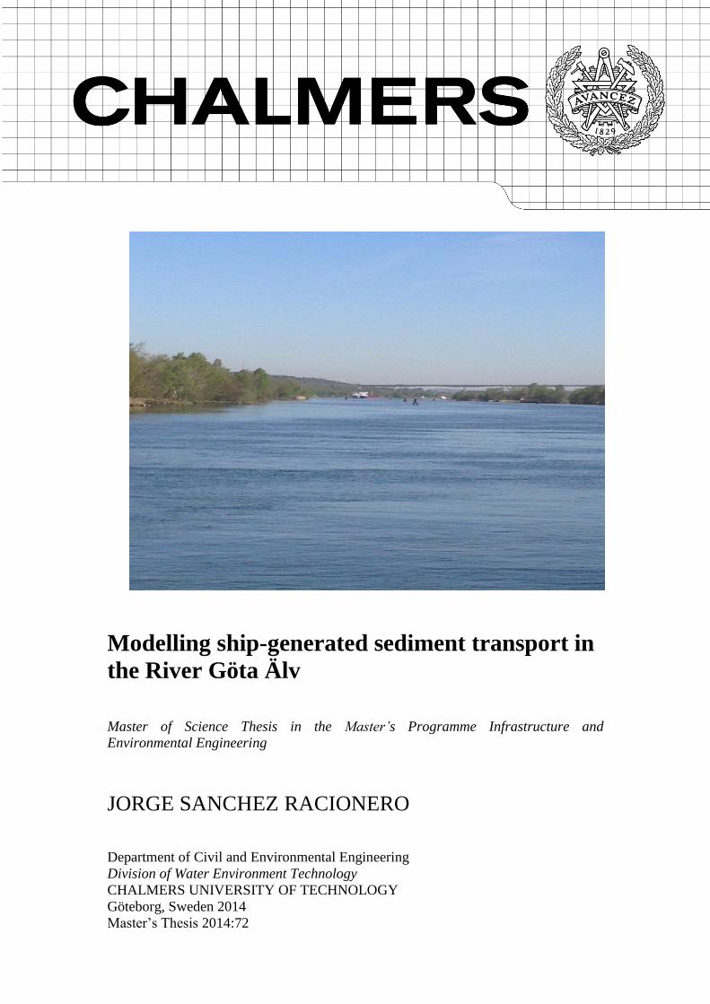
Cover:

An image of a vessel navigating through the River Göta Älv in Lärjeholm (Bondelind

2014).

Chalmers Reproservice / Department of Civil and Environmental Engineering


I

Modelling ship-generated sediment transport in the River Göta Älv






Chalmers University of Technology

ABSTRACT

When a vessel navigates through a natural waterway or a channel, it increases

turbidity in the water body, due to the vessel induced waves, the drawdown, the

vessel-generated currents and the propeller wash. As some heavy metals are easily

attached to suspended sediments, using this water as a source of drinking water can

represent a health risk for consumers.

In the River Göta Älv, the vessel traffic is around 6 000 ships per year, and it is

expected to grow in the future. The river is used as a source of raw water by several

drinking water plants. So the local authorities and drinking water producers in

Gothenburg have interest in predicting the increase of turbidity caused by ship

navigation in the river, for minimizing the health risks for consumers.

In this Master Thesis, a coupled hydrodynamic-sediment transport modelling

approach has been used to forecast turbidity increases after ship passages. The

software used to create the models was MIKE 21 Flow Model FM. A 2D

hydrodynamic model of the River Göta Älv was generated using a flexible mesh

approach. A mesh sensibility analysis was performed to obtain a solution not

dependent on the mesh. Furthermore, validation of the modelled hydrodynamics was

performed. The validation confirmed it was possible to model the river

hydrodynamics satisfactory for any period of the year 2013.

Several ship passages that occurred in the River Göta Älv during 2013 were analysed,

by comparing the turbidity curves measured at Lärjeholm intake and the average

flows measured in the river. Several passages of one ship were selected to be

modelled.

The methodology for modelling ship-generated sediment transport was developed in

this Master Thesis. Coupling the output of the hydrodynamic model with the Mud

Transport module, the transport of sediments generated after this ship passage was

simulated.

The results of the models showed that using the ship-generated sediment transport

methodology the model underestimates the turbidity increase caused by vessels

navigation. Different ideas have been suggested for performing further research.

According to the obtained results, it can be stated that coupling hydrodynamic

modelling with sediment transport modelling is a useful approach for simulating the

increase of turbidity caused by vessels navigation.

Key words: Hydrodynamic modelling, sediment transport modelling, turbidity, vessel,

MIKE 21

II

CHALMERS Civil and Environmental Engineering, Master’s Thesis 2014:72 III

Table of Contents

PREFACE V

NOTATIONS VII

1 INTRODUCTION 1

1.1 Aim 1

2 BACKGROUND 2

2.1 The River Göta Älv study area 2 2.1.1 General description 2 2.1.2 Geology 3

2.1.3 Morphology 3

2.2 Vessels 4 2.2.1 Ship generated waves 4

2.2.2 Squat effect 7 2.2.3 Vessels traffic along the River Göta Älv 8

2.3 Sediment transport processes 8

2.3.1 Transport of sediments caused by environmental factors 9

2.3.2 Transport of sediments caused by ships 10 2.3.3 Suspended sediments in the River Göta Älv 14 2.3.4 Turbidity 14

2.3.5 Estimated total annual transported sediment in the River Göta Älv 14

2.4 Numerical models of sediment transport 15

2.4.1 NAVEFF-SED sediment suspension model 15 2.4.2 Numerical modelling of coupled drawdown and wake 15 2.4.3 Numerical modelling of the sediment re-suspension induced by boat

traffic 16

3 METHODOLOGY 17

3.1 Ship-generated turbidity at Lärjeholm 17

3.2 Hydrodynamic model 17 3.2.1 Mesh generation 18 3.2.2 Initial conditions 20 3.2.3 Boundary conditions 21 3.2.4 Validation 24

3.3 Ship-generated sediment transport model 25 3.3.1 Model set-up 26 3.3.2 Selected ship passage calculations 30

4 RESULTS AND DISCUSSION 34

4.1 Ship-generated turbidity 34

CHALMERS, Civil and Environmental Engineering, Master’s Thesis 2014:72 IV

4.2 Mesh sensitivity analysis results 39

4.3 Hydrodynamic validation results 43

4.4 Ship-generated sediment transport model output 50 4.4.1 Ship passage studied (Case I) 50

4.4.2 Another passage of the same ship for a different date (Case II) 52

5 SUGGESTIONS FOR FURTHER RESEARCH 54

6 CONCLUSIONS 55

REFERENCES 56

APPENDIX I: PRIMARY WAVE DRAWDOWN 61

APPENDIX II: MAXIMUM SECONDARY WAVE HEIGHT 62

APPENDIX III: PROPELLER WASH-INDUCED EROSION 63

APPENDIX IV: NAVEFF-SED SEDIMENT SUSPENSION MODEL 65

CHALMERS Civil and Environmental Engineering, Master’s Thesis 2014:72 V

Preface

This Master Thesis has been performed during the first half of the year 2014. It was

part of the project “Undersökning för att beskriva storlek och dynamik i sedimentbun-

den föroreningstransport i Göta älv”, which was a project carried out by Chalmers

University of Technology, the City of Gothenburg and the Göta Älvs Vattenvårdsför-

bund.

The Master Thesis was performed at “Kretslopp och Vatten” Department of the City

of Gothenburg and at the Department of Civil and Environmental Engineering at

Chalmers University of Technology.

First of all, I would like to thank my supervisors Ekaterina Sokolova, Mia Bondelind

and Olof Bergstedt for their guidance, constructive criticisms and feedbacks during

the project.

For various steps of the modelling process, it was necessary to gather much data. So I

would like to thank the following institutions for their collaborative and helpful atti-

tude providing me with the needed data: the Swedish Maritime Administration, Vat-

tenfall AB, SMHI and Alelyckan drinking water plant.

Besides, I would like to thank Ida-Maja Hassellöv and Fredrik Olindersson, from

Chalmers University of Technology, for providing me with the ship traffic

information (AIS data) used in this Master Thesis.

Also I am grateful to Ulf Olsson and Johan Eriksson, from The Swedish Maritime

Administration, for the data provided by them and the interesting discussion we held.

A special mention is to Angela Liceras Hernandez, for her invaluable help, precise

advices and contributing discussions during this Master Thesis.

Finally, I would like to thank my friends and my family for their help and support

during all the years of hard work at university, especially to my parents, my sister, my

aunt and my grandparents, who have always supported and encouraged me.

Gothenburg, June 2014

Jorge Sanchez Racionero

CHALMERS, Civil and Environmental Engineering, Master’s Thesis 2014:72 VI

Notations

Greek upper case letters

Increased sediment concentration after a ship passage

∆h Water level drop

Total mass per time unit released by the ship

Difference between the mass density of the sediments and the fluid

Diffusion coefficient

Greek lower case letters

Empirical floc erosion rate

Wave diffusion constant

Maximum depth of scour

Bed shear stress

Critical stress of erosion

Critical value below which the mud behaves like a fluid

σ Wave frequency

Water velocity in the horizontal plane

Empirical constant

Dimensionless coefficient dependant on the ship entrance length

Von Kármán coefficient

Kinematic viscosity of fluid

Density of the fluid

Solids weight fraction

Roman lower case letters

River width

Cross-sectional average concentration

Median sediment grain size

Ship draft

Current friction factor

Wave friction factor

Gravity

Water level depth

Total number of point sources

Manning roughness coefficient

Time which takes a point source to release a mass t1 Time span when the increase of turbidity was caused by a ship passage

Wave orbital velocity amplitude at the bed

Shear velocity

vship Ship average speed

Coordinate in the current direction

Distance from the sailing line in the perpendicular direction

Depth of erosion

CHALMERS Civil and Environmental Engineering, Master’s Thesis 2014:72 VII

Roman upper case letters

Area of the river cross-section

River cross section area

BS Ship width

Clearance distance between the propeller tip and the seabed

Concentration of clay released by a point source

Concentration of silt released by a point source

Sediment concentration released by a point source

Sediment concentration just above the bed

Upper concentration limit for free settling

Propeller diameter

Distance between two consecutive point sources

Erosion rate

Length Froude number

Modified Froude number

Densimetric Froude number

Depth Froude number

H Weight height

HM Maximum secondary wave height

Nikuradse roughness parameter

L Wave length

LE Ship entrance length

Distance up-stream from Lärjeholm cross section until where the ship

passage affects the turbidity increase

LS Ship length

Empirical erosion constant

Mass

Sediment mass released by a point source

Proportion of silt fraction

Proportion of clay fraction

Flow released by a point source

Average river flow

Hydraulic radius

Gradient Richardson number

Reynolds number of the jet

Slope of the energy line

Primary wave drawdown

Source flux

Cross-sectional average current velocity

Ship velocity relative to water velocity

Horizontal water velocity component in the horizontal plane

Volume of displacement of water due to ship form

Efflux velocity

Vertical water velocity component in the horizontal plane

Sediment settling velocity

Free sediment settling velocity

CHALMERS, Civil and Environmental Engineering, Master’s Thesis 2014:72 VIII

CHALMERS, Civil and Environmental Engineering, Master’s Thesis 2014:72 1

1 Introduction

Erosion of the riverbanks and the riverbed caused by natural processes has been a

matter of concern for engineering and environmental sciences for many years.

But because of the rapid increase of world shipping commerce produced in recent

years, it has risen up a special concern on studying the effects of vessels navigation in

the natural waterways, such as rivers and navigation channels. Vessels navigation

causes erosion and re-suspension of sediments due to the vessel- induced waves, the

drawdown, the vessel-generated currents and the propeller wash (Trimbak M.

Parchure 2001). All of these effects acting simultaneously set off the erosion and

transport processes, causing an increase of the turbidity in the river water column.

The River Göta Älv flows from Lake Vänern to Kattegat. The river is used as a water

source for supplying drinking water to 700 000 consumers(Sokolova, Pettersson et al.

2013). The river is also used as a waterway for vessels transport. Due to the increase

of vessels traffic occurred during the last years, it has been measured in Alelyckan

monitoring station (Lärjeholm raw water intake) high values of turbidity increase in

the water column after ship passages. Turbidity is utilized as a water quality indicator.

Suspended sediments are the major contributor to turbidity and they are potential

contaminants carrier. Some heavy metals are easily attached to suspended sediments

(Bodo 1989), representing a health risk for consumers. So it has risen up a strong

concern in the drinking water producers and Authorities on minimizing health risks

for consumers associated to ships navigation effects.

To study the turbidity increase generated after ship passages in the river water

column, hydrodynamic modelling and sediment transport modelling are thought to be

useful. Hydrodynamic modelling can be used to describe the temporal and spatial

variability of water conditions in the river occurred after a ship passage. Sediment

transport modelling can describe erosion, transport and deposition of sediments under

the action of currents and waves. The combination of both approaches can be useful to

estimate and predict sediments concentrations after ship passages. It can provide

water producers with a useful tool for assessing health risks related to raw water

contamination.

1.1 Aim

The aim of this Master Thesis was to model the increase of turbidity measured at

Lärjeholm raw water intake after ship passages. Therefore, the area represented by the

models was the stretch of the River Göta Älv from Lilla Edet until Torshamnen.


2 Background

The project requires a well understanding of the River Göta Älv area geology and

morphology, as well as a deep knowledge of the vessel traffic in the river and their

effects on it. Moreover, sediment transport processes and numerical models

simulating these processes need to be studied.

2.1 The River Göta Älv study area

In this section, it is first presented some general information about the case-study area

and then more detailed information about geology and morphology of the River Göta

Älv is presented.

2.1.1 General description

The River Göta Älv rises in Lake Vänern in the southwest of Sweden and discharges

at Kattegat in Gothenburg, western coast of Sweden. The River Göta Älv has a total

length of 93 km, being the largest river in the country (Vattenvårdsförbund 2014). The

basin of the River Göta Älv occupies one tenth of the Sweden land area,

approximately 50 200 km2, which includes the Lake Vänern catchment area as well.

In this study the focus is on the stretch between Lake Vänern and the Sea Kattegat,

compromising an area of 13 300 km2 (Zhang 2009). Lake Vänern is the largest lake in

Sweden and the third largest in Europe. It is located 44 m above sea level and is on

average 27 m deep (Canals 2010). It has a volume of 153 km3, contributing to the

River Göta Älv flow in more than a 90% of the total river flow. The River Göta Älv is

the river in Sweden which has the highest mean flow, with an average water flow of

550 m³/s. The rest of the River Göta Älv flow is originated from local tributaries,

direct runoff of the surrounding areas and groundwater. The travel time from Vänern

Lake to the farthest gauging station (Lärjeholm) varies between 1.5–5 days depending

on the discharge. The discharge from Lake Vänern to the River Göta Älv is regulated

to a maximum discharge of 1 030 m3/s in order to prevent downstream bank erosion

and flooding (Göransson, Larson et al. 2013).

There are 25 tributaries located in the River Göta Älv basin, of which Säveån is the

largest river with a catchment area of 1 475 km². The following largest tributaries

after Säveån are Slumpån, Mölndal, Grönån and Lärjeån, having drainage areas

between 120 and 400km². At the south part of the city of Kungälv, the River Göta Älv

bifurcates into two branches: a northern branch, called the River Nordre, and a

southern branch, still called the River Göta Älv. The River Nordre receives

approximately between 2/3 and 3/4 of the water flow while the southern branch

receives the remaining 1/3 of the water flow (Vattenvårdsförbund 2014).

There are seven measuring stations along the River Göta Älv, distributed from the

Lake Vänern to the Lake Lärjeholm. These stations are Skräcklan, Gäddebäck,

Älvabo, Garn, Södra Nol, Surte and Lärjeholm. In these stations the values of pH,

turbidity, conductivity, temperature and redox potential are analyzed to indicate the

water pollution rate. There is a fixed connection between two of these stations (Surte

and Lärjeholm) and the monitoring data for waterworks are collected at the Alelyckan

drinking water treatment plant control center. In this plant, these data is treated and

analyzed. When high pollution rates are detected, the drinking water plant intake is

closed.

The River Göta Älv is used for drinking water production, transportation, hydropower

production, fish farming and sport fishing. Many municipalities use it as a drinking


water source, supplying nowadays more than 700 000 consumers, among which

Gothenburg is the biggest with approximately 500 000 consumers. Gothenburg has

two different drinking water treatment plants (Lackarebäck and Alelyckan). The raw

water intake is called Lärjeholm and it is placed in the River Göta Älv, (Sokolova,

Pettersson et al. 2013).

The River Göta Älv is regulated by three hydropower stations to generate electricity

as mentioned before. These hydropower stations are located at Vargön, Trollhättan,

and Lilla Edet. Besides, there is a screen facility in the River Nordre to regulate the

river flow and protecting the river from the salt water intrusion coming from the sea

(Poveda 2009). So the water flow in the River Göta Älv is governed by the water level

at the Lake Vänern and the fluctuations of the energy demand.

2.1.2 Geology

The River Göta Älv catchment area is characterized by crystalline bedrock, mainly

gneiss. The soil layers in the River Göta Älv valley consist of clay. The most frequent

type of clay that can be found is glacial clay(SGI 2012). This was deposited in the

vicinity of the melting ice sheet after the glacial period. This glacial clay has a slightly

coarser grain composition than superimposed clays (Sundborg and Norrman 1963).

The River Göta Älv valley is filled with glaciomarine and younger marine clays

(Brack and Stevens 2001), the post-glacial clays. These post-glacial clays were

deposited during a period of fast uplift, when sedimentation took place mainly in a

marine environment within a deep and fairly broad fjord (Sundborg and Norrman

1963). Post-glacial clays in the River Göta Älv valley are mostly present at levels

below 25 m above the sea level. It means that they can be found along the river

downstream Trollhättan. The post-glacial clays layer thickness in the valley is rarely

higher than 15 m. A surface layer (less than 0.5 m) of post-glacial sediments of

varying grain size (clay to gravel) is found in nearly the entire river channel.

Postglacial clay is grey colour, usually unclear and layered. The flat parts of the valley

are often the result of post-glacial clay formed (SGI 2012). In many places, on the top

of the layers there is presence of sandy-silty sediments, which were deposited in fresh

or brackish water conditions (Sundborg and Norrman 1963). In the southern part of

the valley, the thickness of the clay layers increases higher up in the stratification

while sand and silt layers decreases in frequency. Also the presence of fractions of

blocks is remarkable in some specific locations (SGI 2012).

The total thickness of fine sediments in the River Göta Älv valley area is significant.

After different surveys conducted to study the fine sediments layer thickness, it has

been reported that the thickness in Gothenburg is 130 m, at least 54 m in Nol, 50 m in

Lilla Edet, 60 m in Ström, 62 m in Slumpån and in the south of Intagan 55 m

(Sundborg and Norrman 1963).

2.1.3 Morphology

The valley of the River Göta Älv presents two distinct landscapes. One of these

landscapes is located between the municipalities of Tröllhättan and Göta, in the

northern part of the River Göta Älv valley. The other is located between the

municipalities of Göta and Gothenburg, in the southern part of the River Göta Älv

valley.


In the northern part, the old bottom of the fjord raised substantially above the sea level

due to the land uplift produced after the glacial time. In this area, the river cut its way

deep into the clay deposits, creating a relatively narrow furrow with sandy banks of

about 20 m height. The relative height difference between the sediment surface and

the riverbed has a maximum value of 40 m(Sundborg and Norrman 1963). The valley

presents a very variable landscape, with high eroded riverbanks, gully formations and

scars caused by previous landslides.

In the southern part, the riverbanks become lower and lower the more downstream

section the river flows through. The bottom of the valley still retains the original

features of undisturbed sedimentation surface, although there are some scars caused

by previous landslides. In the shallow areas of the river contemporary sedimentation

occurs. This southern part of the valley is at an earlier stage of development compared

to the northern part. The land uplift continues and the progress of erosion is slow. For

this part erosion development is predicted to be similar to the one which has occurred

in the northern part (Sundborg and Norrman 1963).

The erosion process which occurs in the River Göta Älv and in the adjacent areas

contributes to the change in the morphology and stability conditions. During the

second half of the 20th

century five landslides of different sizes have occurred in the

River Göta Älv valley. Here landslides might have been caused by the erosion process

(Hultén, Edstam et al. 2006).

2.2 Vessels

When a ship navigates through a water body, it generates a wave system, and the

propeller jets induce flows into the water mass. This affects the hydrodynamic

conditions in the river. There are many factors which are involved in these

phenomena. Some of these factors are the river flow, the flow velocity and the river

bathymetry. Some other important factors are the ship dimensions, the draught and the

ship speed as well as the factors related to the propeller jets like the number of blades,

the blades area and the propeller revolutions per minute. In very shallow water

conditions, the squat effect can become a serious risk for navigation. To prevent some

risks associated to these effects generated by vessels, some limitations to navigation

have been imposed to ships manoeuvring in the River Göta Älv.

2.2.1 Ship generated waves

A vessel navigating through a homogeneous fluid experiences resistance to motion

caused by viscous and pressure forces generating a wave system in the fluid (Sorensen

1973).

Vessel motion through a water body generates a wave system formed by two different

components (Bertram 2000): the primary component and the secondary component.

The primary waves component is usually referred as drawdown and is caused by the

pressure and the velocity distributions along the ship hull. At the bow and the stern of

the ship an increase of pressure is produced because of the displacement of water,

while in the middle of the ship pressure decreases (Göransson, Larson et al. 2013).

The secondary waves component appears because of the disturbances at the bow and

the stern. The secondary waves include two sets of diverging waves that move

forward and out from the disturbance, and one set of transverse waves that move in


the direction of the disturbance. The divergent waves are also known as Kelvin wake

in honour to Lord Kelvin that was the first person to study them (Sorensen 1973).

The transverse and diverging waves meet a common tangent that forms an angle of

54°44´ with the sailing line of the disturbance. The common tangent point (also called

cusp) has a theoretical amplitude of infinity due to mathematical limitations

(Kostyukov 1959) and form an angle of 19°28´ with the sailing line for all deep water

disturbance speeds (Sorensen 1973).

The sets of diverging waves will travel independently of each other if the bow and

stern are sufficiently separated, but the bow and the stern transverse waves will be

superimposed. The divergent waves travel away from the vessel forming a theoretical

angle of 35°30´ to the sailing line.

At the sailing line, the transverse waves travel at the same velocity as the ship, so the

wave velocity is equal to the ship velocity. Out of the sailing line, the transverse

waves decrease in length and speed (Sorensen 1973).

To describe the characteristics of the wave system created, as well as the physical

processes involved in the generation and subsequent behaviour of the waves, the

following assumptions have to be made for applying the Linearized Wave theory

(Sorensen 1973):

1. The water is homogeneous and incompressible and surface tension forces are

negligible

2. Flow is irrational, the shear stresses at the air-water interface, at the bottom or

at any other solid surface are negligible

3. The pressure at the air-water interface is constant

4. Wave amplitude is small compared the wave depth and wave length

The primary and secondary generated waves can be described by their main

properties, which are the wave height (H), the wave period (T) and the wavelength

(L). There are several factors which affect the wave system generated by a vessel

when it navigates (Kriebel 2005). One of the most important is the type of

environment where the wave system is created, which could be deep or shallow

waters and restricted or unrestricted waters (Rupert Henn 2001). According to the

ratio of the water depth to the ship draft, four categories of environment can be

described according to Vantorre (2003):

Deep water / > 3.0

where is the water depth and is the ship draft

Medium deep water 1.5 < / < 3.0

Shallow water 1.2 < / < 1.5

Very shallow water / < 1.2

The River Göta Älv corresponds to a restricted water body with shallow water

conditions. Other important factors according to Rupert Henn (2001), Bertram (2000)

and to Kriebel (2005) are:

Ship dimensions: ship length LS and ship width BS

Hull design: could be described by the entrance length LE, which is the

distance between the ship bow and the point of maximum ship hull width. The


vessels navigating through the River Göta Älv have in general a short entrance

length (Althage 2010)

Ship draught: Ship velocity (US) relative to water velocity (VR):

Water level depth:

Distance from the sailing line:

River cross sectional area ( )

Volume of displacement of water due to ship form at draft : For characterizing the ship generated waves, two different non-dimensional quantities

(which do not depend on the vessel draft or the design of the underwater body) are

often employed, the depth Froude number ( ) and the length Froude number ( ),

which have the following expressions

√

(1)

√

(2)

where is the acceleration due to gravity. The Froude number used depends on

whether the water is deep or shallow. During many years for deep water conditions it

has been used the length Froude number while for shallow water was used the depth

Froude number. But (Kriebel 2005) stated that in many situations both numbers

should be used to achieve a better characterization of waves regardless of the water

depth and proposed formulas to calculate primary and secondary waves, using a

modified Froude number , defined as:

( )

(3)

where dimensionless coefficient α varies with the hull form and being described as

( ) (4)

where is the ship block coefficient defined as

(5)

The normal block coefficient for tankers is 0.8 while for container ships and ferries is

between 0.5 and 0.7 (Turbo 2011).

When a ship moves at a constant velocity in a rectangular channel of breadth b and

depth h, it has been observed to generate a sequence wave packet called solitons, one

after another, provided that the depth Froude number, , is less than about 1.2

(Ertekin, Webster et al. 1985). In the case study for the River Göta Älv, the depth

Froude number is sufficiently low ( <0.7) in all cases (Göransson, Larson et al.


2013), so solitons are not generated. Thus, these types of waves were neglected in this

Master Thesis approach.

Further information and formulation about the primary wave drawdown ( ) and the

maximum secondary wave height (HM) can be found in Appendices I and II.

2.2.2 Squat effect

A ship in motion creates streamlines of return flow water down the ship sides and

under the ship bottom. These streamlines are specially speeded up under the ship,

causing a drop in pressure which produces a vertical ship sinkage in the water surface.

Besides, the ship generally trims fore or aft. On a ship, trim is the longitudinal

movement experienced by a ship which generates differences between the forward

draft and the after draft. Ship squat is the overall decrease in the static under keel

clearance, which is the distance between the deepest point of the vessel´s hull and the

riverbed. Ship squat is made up of two different components: the vertical ship sinkage

and the trimming effect (Barrass 2004). This phenomenon occurs both in deep waters

and shallow waters. Although in shallow waters, the consequences for navigation

might involve higher risks. Different studies conducted by the Swedish Maritime

Administrations on hydrographical vessels revealed that when the depth below the

keel was higher than five to seven times the vessel draft, the draft increase is not

affected by the bottom depth (Olsson 2009). A ship navigating in a trench navigation

channel will cause the water surface elevation to be lowered because of the increased

velocity which flows around the ship due to the Bernoulli effect (USACE 2006). In

shallow waters, where the static under keel clearance is between 1 or 1.5 m,

grounding due to excessive squat could occur at the bow or at the stern (Barrass

2004).

One of the most important parameters affecting the squat is the block coefficient. A

vessel with a large block coefficient and little or no static trim will normally have a

forward trim. Vessels with block coefficients lower than 0.7 will usually have an aft

trim in shallow water. The initial trim decides whether the vessel bow or stern will be

most affected by squat (Olsson 2009). Although the factor that has the largest

influence on the size of the trim change and the sinkage is the vessel speed (Olsson,

Jakobsson et al. 2008).

A one-dimensional approximation (Blaauw 1984) can be used to calculate the

resulting water level drawdown. The lowering of the water level (or drop, ∆h) is equal

to the mean ship sinkage and therefore the squat (USACE 2006), expressed as

follows:

(

( ) )

(6)

where


2.2.3 Vessels traffic along the River Göta Älv

The River Göta Älv has been since ancient times an important waterway for both

commercial and recreational boats. There is a traffic between 2500 and 2700 of

commercial ships per year and about 3500 recreational boats per year(Hultén, Edstam

et al. 2006).

Due to manageability and safety reasons, there are restrictions to the dimensions of

the vessels navigating the river. It is limited to a maximum length of 89 m, maximum

width of 13.4 m and a maximum draught of 5.4 m. Allowed maximum draught may

vary depending on the water level.

Vessels which navigate through the River Göta Älv must fulfil some speed

restrictions imposed by the Swedish Maritime Administration. The maximum allowed

speed in the canal is 10 knots (between Lärje and Dalbo bridge), with some areas

where allowed speed is lower (varying from 5 to 7 knots).

2.3 Sediment transport processes

Sediments present at the riverbanks and the riverbed usually have a wide range of

sediments types, ranging from gravel and coarse sand (known as non-cohesive

sediments) to fine particles like clay or silt (known as cohesive sediments) (Trimbak

M. Parchure 2001). Non-cohesive sediments form a rigid bed upon deposition, so the

erosion rate can be related directly to the flow properties and the diameter of the

sediments (Van Maren, Winterwerp et al. 2009). Cohesive sediments sometimes

include organic-rich sediments and waste materials. Cohesive sediments are strongly

affected by the negative charge of its particles, resulting in a slow formation of a soft

consolidated bed, where the interstitial pore water is expulsed over the time.

Flocculation occurs for cohesive sediments, attaching particles and boosting the

formation of flocs. Flocculation is affected by the type of particle, its natural

properties, some biological processes and the hydrodynamic conditions (Willis and

Krishnappan 2004).

Mashriqui (2003), following the theory presented by the U.S. Interagency Committee

on Water Resources, Subcommittee on Sedimentation (1957), provided the fall

velocity characteristics of sediments for different grain size and characteristics in 20° C water temperature conditions:

Table 1. Sediment size and settling velocity

Sediment Type >Grain

Diameter (mm)

<Grain Diameter (mm)

Average Diameter (mm)

Settling Velocity

(m/s)

Clay 0.0020 0.0040 0.0030 0.00002

Very Fine Silt 0.0040 0.0080 0.0060 0.00006

Fine Silt 0.0080 0.0160 0.0120 0.00019


Medium Silt 0.0160 0.0320 0.0240 0.00050

Coarse Silt 0.0320 0.0625 0.0473 0.00150

Very Fine Sand 0.0625 0.1250 0.0938 0.00350

Fine Sand 0.1250 0.2500 0.1875 0.00700

Medium Sand 0.2500 0.5000 0.3750 0.01700

Coarse Sand 0.5000 1.0000 0.7500 0.02800

Very Coarse Sand

1.0000 2.0000 1.5000 0.04200

2.3.1 Transport of sediments caused by environmental factors

The transport of sediments in a river is mainly caused by the current of the river,

which drags the suspended material in the water column, although there are other

environmental processes affecting the sediments transport (wind force, presence of

aquatic plants, artificial barriers and landslides). Sediment discharge into a river can

have two different pathways: the stream channel sediment transport (bed load,

suspended load and wash load) and land surface transport (mass movement). Each of

these contributions of sediments has a different time scale, requiring the surface

transport much more time to develop than the stream sediment transport (Mouri,

Shiiba et al. 2011).

The transport processes for the cohesive and non-cohesive sediments are very

different. The most important parameters affecting the non-cohesive sediment

transport are particle size, density and critical shear stress for incipient motion (Marin

2005). In the case of cohesive sediments, the size and density of the cohesive

sediment particles themselves become dependent variables. In addition, particle

mineralogy, the electrochemical nature of the flowing medium and biological factors

such as bacteria content and other organic material are important factors (Willis and

Krishnappan 2004).

When matter is transported in a river, it is spread due to dispersion caused by

turbulent diffusion perpendicular to the dominant longitudinal current direction in

combination with velocity variations over the cross section. The effect of dispersion in

the longitudinal direction can be described by the one-dimensional advection-

diffusion equation, which has the following expression (Bergdahl and Bondelind

2013):

(7)

where

( ): Concentration of a substance, cross-sectional average

: Coordinate in the current direction, measured downstream from the releasing point


: Current velocity, cross-sectional average

: Longitudinal dispersion coefficient, which according to Fischer, Imberger et al.

(1979), in natural watercourses it is mainly governed by horizontal velocity

differences. It can be estimated as follows:

(8)

where

: River width

: Water depth

: Shear velocity, having the following expression for turbulent flow conditions in a

wide channel:

√

where

: Slope of the energy line, which has the following expression

⁄

where

: Manning roughness coefficient

: Hydraulic radius, which can be calculated as

: Area of the river cross-section

A solution for Equation 7 in the case of instantaneous release of the mass in the

point m at the time t=0 s, is the following:

( ) ⁄

√ ( ( )

)

(9)

2.3.2 Transport of sediments caused by ships

When vessels navigate through a river, the generated flows are variable in quantity

and direction, affecting the river flow. Due to these turbulences in the river flow, the

time available for the sediment consolidation process is short. A very thin and easily

erodible layer (some few centimeters in thickness) is formed at the surface, creating

the erosion, deposition and consolidation sediments cycle (Trimbak M. Parchure

2001). This thin layer between the water column and firm bed has a high content of

water and very low cohesive shear strength. This thin layer can suffer two modes of

failure. The first, called surface erosion, appears due to the floc-by-floc rupture and

entrainment of the surficial sediment. The second, called mass erosion, is caused by

dynamic shear loading of the bed. In this case, the plane of failure lies deep in the bed


and the failure results in a fast entrainment of the sediments above the plain

(Partheniades 1982).

2.3.2.1 Wave generation by moving vessels

The waves, possibly in combination with the river current, mobilize material from the

bed, bringing it up into the water column. A concentration profile develops depending

on the forcing conditions and the properties of the sediment. As the waves decay, the

material settles again, at a low rate because of the fine grain sizes prevailing

(Göransson, Larson et al. 2013).

In open areas, the primary waves generated by the navigation of vessels tend to have

less influence on the bed and bank sediments than in restricted waterways. However,

the drawdown produced has a higher relevance in restricted waterways due to the

effects that it has on the bed and bank sediments (Göransson, Larson et al. 2013).

Drawdown could generate large particle velocities at the bed because of long

wavelength; and after shoaling, it will create large wave heights at the shoreline. The

ratio between the cross-sectional areas of the vessel and of the waterway shows the

importance of the drawdown effects in a restricted waterway. The smaller this ratio is,

the smaller the effects of the drawdown are.

2.3.2.2 Propeller wash-induced erosion

As a direct consequence of the increase in the size and the speed of seaborne

transport, vessels have been upgraded with higher installed engine capacity and

increased manoeuvrability. Large-diameter propellers and bow thrusters create an

increase of the wash on the bed and the banks of harbour basins and navigation

channels (Hong, Chiew et al. 2013). Propeller-wash induced erosion does not

represent a serious risk itself in open water bodies. But if this erosion takes place in

harbours, it can damage the maritime structures and induced a risky situation (Hashmi

H. N. 2007). Therefore, there has been an increasing interest in studying the

characteristics of the propeller-induced scour because of its erosive power (Hong,

Chiew et al. 2013). It could damage the quay structures affecting the structures

stability, ultimately leading to its failure (Hashmi H. N. 2007).

Different methods have been developed to approximate the maximum depth of scour

for a specific wash configuration in situations without berth structures present. In this

report, the methodology developed by (G. A. Hamill 1999) is presented, who

conducted an extensive study of the scouring action of a range of propellers. These

equations have a limited applicability since they were formulated for conditions which

assume that the propeller wash was generated in unobstructed conditions, where free

expansion could take place. In the case of the River Göta Älv, the conditions in the

sailing line are unobstructed for the vessels, so the equations described in Appendix

III have full applicability. The maximum depth of scour ( ) is function of the

following variables:

( ) (10)

: Efflux velocity

: Propeller diameter


: Median sediment grain size

: Clearance distance between the propeller tip and the seabed

: Density of the fluid

: Acceleration due to gravity

: Difference between the mass density of the sediments and the fluid

: Kinematic viscosity of fluid

A complete build-up of the equations can be found in Appendix III.

2.3.2.3 Bed shear stress

Disturbances generated by vessels navigation through a river can cause erosion and

re-suspension of sediments. Erosion or re-suspension of bottom sediments is one of

the most important factors controlling fine sediment transport in natural water bodies

(Sanford and Maa 2001). The shear stress at the sediment-water interface is a decisive

factor in the sediments erosion and transport processes (Jepsen, Roberts et al. 2012).

The action of the waves generated by vessels produce bed shear stresses, which may

or may not result in sediment suspension depending on the relative magnitudes of the

wave-induced bed shear stresses. Shear strength of cohesive sediment bed increases

with increasing bulk density (Trimbak M. Parchure 2001). There are different site-

specific sediment characteristics which oppose the shear stresses at the riverbed

generated by vessels waves and currents. Several of these sediments characteristics

are the particle size distribution, cohesiveness, particle density, water content (or bulk

density) and binding (or biological disturbance) (R. Jespen 1997) and (Sanford and

Maa 2001).

According to (Sanford and Maa 2001), the erosion process can be classified in Type I

and Type II erosion. Type I erosion occurs when the bed critical stress for erosion ( ) increases with the depth into the sediments, limiting the extent of erosion. Type II

erosion means that has a constant value which does not change with the sediments

depth.

Power law erosion formulation for Type I erosion is

( [ ( )] ) (11)

= Erosion rate

= Empirical floc erosion rate

and = Empirical constants

= Applied shear stress

= Critical stress of erosion

= Depth of erosion

Erosion formulation used for Type II is the following simple linear relationship

( ) (12)

= Empirical erosion constant


Rydell, Persson et al. (2011) measured the values of the erosion constant ( ) for

different sections of the River Göta Älv, obtaining the following values:

Table 2. Erosion Constant measured in different sections of the River Göta Älv

Section of the River Göta Älv Erosion constant ( ),

[Kg/m2/s]

Vänern - Lilla Edet 1, 97 x 10-7

Lilla Edet - Bohus 6, 66 x 10-7

Bohus – Nordre Älv fjord 3, 59 x 10-6

Bohus – Göteborgs hamn 2, 60 x 10-5

Rydell, Persson et al. (2011) classifies the bottom of the River Göta Älv in five

different classes according to their bottom behavior. There are materials which tend

to sediment and others which tend to be eroded and/or transport in the bottom.

Attending to this classification, Rydell, Persson et al. (2011) in their report calculated

the value of the critical shear stress ( ) for the River Göta Älv, as presented in Table

3.

Table 3. Type of materials present in the River Göta Älv riverbed, their probable

behaviour and the critical shear stresses

Bottom class

Assessed materials Probable bottom

behaviour Critical shear

stress ( ), [Pa]

Class 1 Very loose sediments (clayey mud, muddy

clay) Sedimentation bottom 0.34

Class 2 Loose sediments (clay,

mud, silt, organic material)

Sedimentation bottom 0.36

Class 3 Fine sand, silt, hard clay,

organic matter Among the bottom 0.37

Class 4 Between sand, coarse

sand Erosion and /or

transport bottom 0.51

Class 5 Gravelly sand, gravel,

stone Erosion and /or

transport bottom 0.76

The decrease in the erosion rate of stratified beds occurs due to increase of the

cohesive shear strength in comparison to the erosion of the bed with respect to depth.

Erosion is detained where the bed shear stress ( ) equals the bed shear strength. This


value of is equal to the critical shear stress ( ) at that depth. increases with bed

consolidation time, resulting in a decrease of the erosion rate (Partheniades 1982).

2.3.3 Suspended sediments in the River Göta Älv

Rydell et al. (2011) made a classification of the suspended sediments according to the

transport behavior in the river bed and the water flow. These four groups are:

Wash load. Particles which has no contact with the bottom of the river. They

only are transported by the river flow.

Suspended load. Particles which are transported by the river flow as the wash

load, but have contact with the bottom of the river.

Dissolved load. Particles which are present in the water body with a very small

size.

Bed load. Material which suffers a friction process during the transport

process.

2.3.4 Turbidity

Turbidity is the cloudy appearance of water which is caused by suspended material

(Consulting 2010) . There are many sources which provide suspended material to the

rivers, creating turbidity in the water body. The tributaries of the river bring

suspended sediments, as well as the precipitation runoff of the surroundings. Besides,

the erosion of the riverbed and the river banks caused naturally or by human action

also contributes.

The measured turbidity reflects the suspended sediment concentration (SSC), but the

relationship between SSC and the turbidity is typically complex (Göransson, Larson

et al. 2013).Turbidity is strongly correlated to settlement time of the eroded material

and the particle sizes. It is very site specific and without laboratory measurements of

samples from the specific site, the estimation of relationship between the turbidity

levels (FNU) and the total suspended sediments (mg/L) is uncertain (Consulting

2010).

Althage (2010) conducted a sampling campaign in the River Göta Älv at Garn station,

in which several samples were taken. The suspended sediment concentration and the

turbidity were analysed simultaneously. An approximately linear relationship was

obtained were 1 mg/l of SSC corresponded to a turbidity of 1 FNU.

2.3.5 Estimated total annual transported sediment in the River Göta

Älv

The most common sediment transport in the River Göta Älv is the one generated by

the erosion which occurs in the river banks (Göransson and Persson 2011). An

estimation of the total annual transported sediment in the River Göta Älv stated a

quantity between 130 000 and 170 000 tons. Approximately, the 40% of it leaves

through the southern branch (Göta Älv) (SGI 2012).

Althage (2010) conducted calculations of the total annual erosion due to ship passages

effects in the River Göta Älv, taking water samples from the river for turbidity

measurements. These estimations where calculated using the relationship between

SPM and turbidity. It was supposed that the annual number of vessels navigating the


River Göta Älv would be 1600, an affected river width of 11 m and the total length of

the River Göta Älv (93 km) affected by vessels motion. The total annual eroded mass

caused by vessels motion was estimated in 40 000 tonnes.

2.4 Numerical models of sediment transport

Different approaches have been developed by several authors aiming to model the

hydrodynamics induced by ships moving and the sediment transport caused by vessels

in natural flows. Some of the models used in this document to get a close

understanding of how this phenomenon can be modelled are presented here.

2.4.1 NAVEFF-SED sediment suspension model

The desktop computational procedure NAVEFF-SED developed by Trimbak M.

Parchure (2001) is presented here to give an estimation of depth-averaged sediment

suspension concentration representing simplified natural conditions under vessel

generated waves and the shear stresses produced at the riverbed. It takes into account

the sediment settling and deposition plus erosion from the bed and the upward

diffusion by short period waves and/or superposed current, as it is the case study for

the River Göta Älv. This methodology can be applied both to cohesive and non-

cohesive sediments under a variety of conditions and parameter selection.

A complete build-up of the NAVEFF-SED model equations can be found in Annex

IV.

2.4.2 Numerical modelling of coupled drawdown and wake

MacDonald (2003) developed the Ship-Generated Hydrodynamics (SGH) computer

model in order to predict the effects of deep-draft vessel traffic. This model does not

include any approach to the sediments transport, although provides a good

understanding of the vessel generated hydrodynamics. The SGH model is comprised

of two dynamically-coupled sub-models, one for the wake and one for the drawdown,

which calculate vessel-generated water surface fluctuations, current velocities and

wake transformation. The model uses a finite difference technique approach to

separate the vessel-induced flow mathematically into a high frequency component, the

wake, and a low frequency component, the drawdown, during the temporal integration

of the equations of motion. After integration over the depth, this results in the

standard shallow water equations (conservation of mass and momentum) for the

drawdown.

The model is constructed to permit the use of complex channel geometry and

bathymetry, realistic ship hull shapes and variable sailing lines, and employs an auto-

calibration technique to ensure accurate wake generation.

This computer model has been used successfully and cost-effectively on a number of

projects in Canada and the US.


2.4.3 Numerical modelling of the sediment re-suspension induced by

boat traffic

A 1DV model was set up in a study conducted by Smaoui, Ouahsine et al. (2011) to

model the sediment re-suspension induced by vessels traffic in the "Canal de la

Sensée" (north of France) and in the Seine River. The 1DV model was obtained by

neglecting all the horizontal gradients, except the pressure gradient. It is based in a set

of equations for the mean and turbulent movements and the continuity equation. The

propeller effects were neglected in the calculations.

To evaluate how different passing boats impact on the waterway, field measurements

of the hydraulic conditions (the water elevations close to the bank and the flow

velocities in the vicinity of the bottom) and the solid suspended matter concentrations

(SSM) were made at different points.

The 1DV model supplies information on turbulence, bottom stress shear and

sedimentary flux.

Despite of its apparent simplicity, the model considered all the governing processes

(hydrodynamic, turbulence, sediment transport) to compute the boat induced sediment

transport.


3 Methodology

In this chapter the ship-generated turbidity increase at Lärjeholm is described.

Furthermore, this chapter describes the approach used to represent the hydrodynamics

of the River Göta Älv using a computational model. It provides a description of how

the hydrodynamic model has been setup and how the computational mesh has been

generated. Furthermore, it explains the mesh sensitivity analysis and the

hydrodynamics validation process followed. Finally, it states the methodology

developed for modelling the ship-generated sediment transport in the river.

3.1 Ship-generated turbidity at Lärjeholm

To determine the generated turbidity caused by a ship passing Lärjeholm, data on

turbidity, ship passages and flow conditions have been compared. Data from year

2013 has been evaluated. The turbidity values are continuously measured at the

Lärjeholm measuring station. These data were provided by “Kretslopp och Vatten”

from Gothenburg city. Data on water flow in the river in the Göta Älv branch were

provided by Vattenfall (Vattenfall 2013). Data on ship passages were retrieved from

AIS data on ship navigation provided by The Swedish Maritime Administration

(Sjöfartsverket 2014).

Different ships have passed the River Göta Älv during the year 2013. Some examples

of these ships are Walona, Origo, Bristol, Nordic Sina, Patria and Shetland Cement. It

was, however, not possible to evaluate all ship passages within the scope of this

thesis.

The aim was choosing a turbidity increase occurred after a ship passage that could

clearly be correlated with the ship passage. Also, it was intended to choose this

turbidity peak during a medium-high turbidity period in the river, because of the

interest that the drinking water producers in Gothenburg city had in studying these

turbidity peaks, for water quality reasons. Besides, it was intended to select a ship

with the biggest dimensions allowed to navigate through the River Göta Älv,

especially with the maximum allowed draught (5.4m).Furthermore, only upstream

passages were studied because they are the ones which create the highest turbidity

increases because of navigating against the river current direction.

So after studying several ship passages in different time periods during the year 2013,

it was decided that the ship Patria was the one which fulfil better these requirements.

Therefore it was the ship chosen for modelling the turbidity increase after its passages

in Lärjeholm cross-section. Patria ship dimensions are: a draught of 5.4m, a length of

82m and a breadth of 13m.Its gross tonnage is 2210 t and its dead weight is 3519t. It

was built in 1995 (MarineTraffic 2014). This ship navigated quite often through the

River Göta Älv during year 2013 (nearly once every 10days) (Sjöfartsverket 2014).

3.2 Hydrodynamic model

The hydrodynamic conditions in the River Göta Älv were modelled using the

simulation software MIKE 21 Flow Model FM (Flexible Mesh) developed by DHI.

The model is based on the numerical solution of the two-dimensional shallow water

equations, the depth-integrated incompressible Reynolds averaged Navier-Stokes

equations. The model consists of continuity, momentum, temperature, salinity and

density equations. The spatial discretization of the primitive equations is performed


using a cell-centered finite volume method. The spatial domain is discretized by

subdivision of the continuum into non-overlapping elements. In the horizontal plane

an unstructured grid is used comprising of triangular elements. An approximate

Riemann solver is used for computation of the convective fluxes. For the time

integration an explicit scheme is used (DHI 2012).

3.2.1 Mesh generation

For obtaining reliable results from the hydrodynamic model of the River Göta Älv, it

was essential to provide the software with a suitable mesh. This mesh had to represent

with an adequate resolution the bathymetry of the river and the flow fields as well as

the river boundaries. Assigning the right geographical position to each node in the

mesh was crucial to represent the hydrodynamic river conditions.

Mesh generation was carried out using MIKE Zero Mesh Generator. Using this tool, a

flexible mesh (consisting of triangles in the horizontal plane) was generated (DHI

2012). GIS data files provided by the Swedish Geotechnical Institute (SGI) and by the

Swedish Maritime Administration (Sjöfartsverket) were used to define the bathymetry

and the contour of the River Göta Älv in the mesh. The map projection used was

SWEREF99 TM. The contour of the river was defined by nodes and arcs (which

assembled these nodes). The mesh was created with 46 098 nodes and 84 268 mesh

elements (triangles) in the horizontal plane. In the vertical plane, for each triangle it

was made an interpolation of the GIS bathymetry data contained in that triangle,

assigning an average depth to each. The domain used in the model covered the area

between the municipality of Lilla Edet and the mouth of the River Göta Älv in

Torshamnen. The branch Nordre Älv, when the River Göta Älv bifurcates in

Kungsälv, has not been included in the mesh. The domain used in the model and a

detailed view of the mesh at Lärjeholm are represented in Figures 1 and 2

respectively.

Figure 1. Mesh used to model the River Göta Älv in the stretch between Lilla Edet and

Torshamnen.


Figure 2. Detailed view of the mesh at Lärjeholm

The length of the mesh triangles sides varied from approximately 10m to 37m. The

smallest triangle angle was 26°.

3.2.1.1 Mesh sensitivity analysis

The resolution of the mesh is a trade-off between quality of the model and

computational time needed to run simulations. The smallest mesh elements as well as

the number of mesh elements condition the simulation time (DHI 2012).

Due to the critical influence of the mesh on the model results, a mesh sensitivity

analysis was performed. The purpose of this sensitivity analysis was to have a

solution that was not dependant on the mesh, with a reasonable computational time.

To evaluate the effect of the mesh on the modelling results, three different parameters

(water surface elevation and the two water velocity components in the horizontal

plane, U and V) were compared in three different locations along the river using four

different meshes. The coordinates of these locations in the reference frame

SWEREF99 are the following:

Agnesberg: (6409032.65; 322135.21)

Lärjeholm: (6406611.18; 321799.92)

Eriksberg: (6399658.38; 316879.51)

Successive mesh refinement was carried out. The same bathymetry and river contour

data were used for all meshes.

When using MIKE software to generate a mesh it is not possible to choose the number

of elements in the mesh. It can only be chosen the maximum mesh element area and

the smallest mesh element angle. So choosing different maximum mesh element area

and the smallest mesh element angle, several meshes were created. The information

on these meshes can be seen in Table 4.


Table 4. Meshes characteristics used in the mesh sensitivity analysis

Mesh type Number of

mesh elements

Number of mesh nodes

Min triangle

side length

[m]

Max triangle

side length

[m]

Max triangle

area

[m2]

Smallest triangle

angle

[°]

Coarse mesh 21 068 12 525 20 70 1000 26°

Intermediate mesh

42 263 23 959 17 56 500 26°

Fine mesh 84 268 46 098 10 37 250 26°

Very fine mesh

105 332 57 126 7 25 200 26°

The four models calculated had the same initial conditions, same boundary conditions

and same sources (tributaries of the river), differing only in the mesh. The period

modelled had a duration of three days, from 09/08/2013 at 00:00:00 until 12/08/2013

at 00:00:00, with a time step of 10 minutes.

3.2.2 Initial conditions

The initial conditions used for all the models have been the water surface elevations

of all the points of the domain at the first step of the simulation. The water level

depends on the water flow, so each modelled period had its own initial conditions file.

These initial conditions files were Grid Series files.

The data used to create the initial conditions files were the surface elevations at the

boundaries Lilla Edet and Torshamnen. The initial surface water level data in Lilla

Edet were acquired from Vattenfall and in Torshamnen from the Swedish

Meteorological and Hydrological Institute (SMHI). The initial surface elevation

values for the rest of the mesh nodes were specified by interpolation between the

values of these two boundaries.

In Figure 3, it can be seen an example of the initial conditions for one of the models

which has been simulated. This model represented Medium Water Flow conditions

during 2013. The average water flow in this case was: 490 m3/s at Lilla Edet, 340 m

3/s

in Nordre Älv and 150 m3/s in the Göteborg branch.The period modelled had a length

of three days, from 09/08/2013 at 00:00:00 until 12/08/2013 at 00:00:00, with a time

step of 10 minutes. The water level used for initial conditions in Lilla Edet was 0.37

m and 0.098 m in Torshamnen.


Figure 3. Initial conditions file with the nodes surface elevation for a Medium Water

Flow conditions model (from 09/08/2013 at 00:00:00 until 12/08/2013 at 00:00:00)

3.2.3 Boundary conditions

In all the models created, the entire river contour was modelled as closed boundaries

to represent the interface land-water (land boundaries), except for three areas which

were considered open boundaries.

In the closed boundaries, normal fluxes were forced to zero for all variables.

The three open boundaries were located as follows: the inlet at Lilla Edet, the outlet at

Nordre Älv and the outlet at Torshamnen. All the open boundary conditions files

were Time Series files.

The boundary conditions at Lilla Edet and at Nordre Älv were defined by the water

flows (specified discharge), with hourly time step. The water flow data at Lilla Edet

and at Nordre Älv were acquired from Vattenfall. A Time Series file example

containing the water flows in Lilla Edet and in Nordre Älv files can be seen in Figure

4, following the same example shown above in Section 3.2.2. The water flow values

in Nordre Älv are negative because the flows came out of the model.


Figure 4. Time Series file created to represent the water flow variations in Lilla Edet

and Nordre Älv boundaries from 09/08/2013 at 00:00:00 until 12/08/2013 at

00:00:00, with a time step of 1 hour.

The boundary conditions at Torshamnen were defined by the water surface elevation

and the water velocity components in the horizontal plane ( and velocities) with

hourly time step which covered the whole period of each model simulation. These

types of boundary conditions are called flather conditions in the models.

The water velocity components in the horizontal plane ( and velocities) at

Torshamnen were calculated with hourly time step, with values which covered the

whole simulation period. For these calculations the water flow data (acquired from

Vattenfall) and the total area of Torshamnen cross-section (6160m2) were used.

Assuming that the horizontal water velocity (v) formed 190° with the X-axis (Figure

5), the formulas used to calculate the velocity components for each time step in each

model were:

(13)

( ) (14)

( ) (15)

where

: Water velocity in the horizontal plane

: Horizontal water velocity component in the horizontal plane


: Vertical water velocity component in the horizontal plane

: Water flow in Torshamnen cross-section

: Cross-section area in Torshamnen

Figure 5. Horizontal water velocity component (v) at Torshamnen, which forms with the x-axis.

The water surface elevation data in Torhamnen were acquired from SMHI. To input

these water surface elevation data into the models, it was followed the same

methodology described above for the boundaries Lilla Edet and Nordre Älv. In Figure

6 it can be seen an example of a surface elevation Time Series file which was created.

Figure 6. Time Series file created to represent the water surface elevation in

Torshamnen boundary from 09/08/2013 at 00:00:00 until 12/08/2013 at 00:00:00,

with a time step of 1 hour.


3.2.3.1 Tributaries

The River Göta Älv area which has been modelled, located between Lilla Edet and

Torshamnen, includes several tributaries, but in these models only the six tributaries

which have the highest flows (Gårdaån, Grönån, Lärjeån, Säveån, Mölndalsån and

Haltorpsån) were incorporated (Figure 7).

Figure 7. Flows from tributaries of the River Göta Älv during 2013 (created with

SMHI provided data)

The tributaries were included into the hydrodynamic models as point sources with

continuous variable flow, using the data acquired from SMHI. The tributary flow data

was provided with daily values, so before the setup of each hydrodynamic simulation,

time series files had to be created for each tributary, representing the continuous

discharge of every tributary.

3.2.4 Validation

The hydrodynamic model is the base model in which the sediment transport model

will be implemented. So for ensuring that hydrodynamics were solved in a precise

mode and not interfering in the sediments transport results, a hydrodynamics

validation process was performed.

The validation of hydrodynamics was done by comparing measured and simulated

water levels in different locations along the River Göta Älv for different models,

which represented different water flow conditions in the river for the year 2013.

Three different periods were modelled, creating three different models with 3 days

simulation time each. The aim was to represent three different water flow conditions

in the River Göta Älv during year 2013. The first period represented high flow water

conditions (from 03/03/2013 at 00:00:00 until 06/03/2013 at 00:00:00), the second

period represented medium flow conditions (from 09/08/2013 at 00:00:00 until


12/08/2013 at 00:00:00) and the third period represented low flow conditions (from

23/10/2013 at 00:00:00 until 26/10/2013 at 00:00:00) (Figure 8).

Figure 8. River Göta Älv water flow during year 2013 measured in Lilla Edet cross-

section. The red, orange and yellow lines show the three different periods modelled to

conduct the hydrodynamics validation.

The water levels measured in four different locations of the River Göta Älv were

compared with the water levels outputs of the three different models. The coordinates

of these four locations in SWEREF99 projection are the following:

Agnesberg: (6409032.65; 322135.21)

Lärjeholm: (6406611.18; 321799.92)

Tingstadstunneln: (6401740.89; 320579.61)

Eriksberg: (6399658.38; 316879.51)

A map showing these locations can be seen in Figure 9.

Figure 9. Map showing the four locations where validation of hydrodynamics has

been performed.

3.3 Ship-generated sediment transport model

When a vessel navigates through a river, it generates turbulences in the river flow,

creating usually an increase of turbidity in the water column (for further information

see Section 2.2 and Section 2.3.). In this section the methodology developed to model

the ship-generated sediment transport in a river is presented. Furthermore, this


methodology is applied to study one ship passage occurred in the River Göta Älv

during year 2013.

3.3.1 Model set-up

The ship is assumed to continuously stir up sediment while traveling up the river,

Figure 10. In the model (Figure 10), it is assumed that ship-generated sediments

(turbidity increase) can be described by a system of point sources of sediments (Si).

The sources are placed at discrete points along the river with a distance . Each point

source discharge a sediment mass , every , times. It represents the

increase of sediments concentration in the water column caused by the ship passage

travelling upstream the river.

The model is set-up by coupling the 2D hydrodynamic model of the river with the

MIKE Mud Transport module. The erosion process in the river and other sources

providing sediments to the river have not been considered in this model. The

calculations for Si, , and are further described in the following

sections.

Figure 10. System of sediment point sources used to model the turbidity increase

generated by a ship passage and measured at Lärjeholm intake after the instant the

ship navigated through this cross section ( ) .

In MIKE 21, there are three types of sources: simple, standard and connected sources.

The sources used in the model in this thesis were simple sources. This means that

each point source contribution to the continuity equation was taken into account in the

hydrodynamic model. If the magnitude of the source is positive, water is discharge

into the ambient and if the magnitude is negative, water is discharged out of the


ambient water (DHI 2012). In the models developed here, all the point sources

magnitude was positive. It means that all sources discharged a positive flow ( ) into the model.

Each point source of the model was implemented into the software using a source flux

(SF), as follows (DHI 2012):

[kg/s] (16)

: Flow of the point source [m3/s]

: Sediment concentration of the point source [kg/m3]

See Section 3.3.1.4 for and calculations.

3.3.1.1 and

The sediments concentration and flow released by each point source were correlated

to the turbidity increase measured at Lärjeholm after ship passages (turbidity data

provided by “Kretslopp och Vatten”, from the City of Gothenburg). For calculations,

it was used the relationship between the increase of sediment concentration ( )

and turbidity measured in the River Göta Älv at Garn station by Althage (2010): 1

mg/l of SSC corresponded to a turbidity of 1 FNU. Although this relationship is very

time and site specific. So, if in future research it is available data from Lärjeholm

cross section, it is advised to be used.

The value of was calculated approximating the area enclosed by the turbidity

curve and the horizontal T2 axis (Figure 11) with a rectangle of the same area, whose

sides were and . The origin of coordinates is placed at a turbidity of 0

FNU and a time of T1=T2=0 s (instant when the ship navigated through Lärjeholm

intake cross section). The horizontal T2 axis is the horizontal T1 axis displaced a

distance Turbinit , which is the turbidity value measured when the ship navigated just

through Lärjeholm intake section. is the time that, according to the rectangle

approximation made, the ship generated the increase of turbidity . The creator of

the model must choose for each model.

t1 is the time span when the turbidity increase is assumed to have been caused only by

the ship passage. After the time t1, turbidity values measured at Lärjeholm are caused

by different reasons than the ship passage, as it could be the runoff coming into the

river or the natural re-suspension of sediments caused by the river current. t1 must also

be decided by the model creator studying the turbidity curve and deciding until when

the turbidity increase was produced only by the ship passage effects.


Figure 11. Scheme showing the rectangle ( and sides) used to

approximate its area to the area enclosed by the turbidity curve and the horizontal

time axis T2 .

In the methodology developed in this Master Thesis, it was assumed that

measured at Lärjeholm raw water intake was the concentration of the entire cross

section after the ship passage. Multiplying by the average river flow ( ) measured in

the river, it was obtained the total sediments mass per time unit ( ) released by

the ship.

: Sediments mass increase per time unit [kg/s] (17)

3.3.1.2 Distance and

is the distance between consecutive point sources(Figure 10), assuming that the

ship speed was vship. This distance had to be decided by the model creator, taking into

account that there is a minimum limit distance, due to the model mesh triangles size.

So should always be higher than this minimum value to avoid placing two point

sources in the same mesh cell.

vship is the average speed of the ship chosen to be modelled when it navigated through

the study stretch of the river. It is calculated using the AIS data (provided by The

Swedish Maritime Administration). It took the ship a time to navigate between

two consecutive point sources.

[m/s] (18)

𝐶𝑠𝑒𝑑

Turbinit

𝑡𝑆𝑜𝑢𝑟𝑐𝑒

t1

T1

T2

Turbidity [FNU]


3.3.1.3

is the total sediment mass released by one point source in each release. This

mass represents the turbidity increase generated by the ship passage through all the

cross sections during a period of time , in which the ship navigated through these

sections (Figure 10). had the following expression:

[Kg] (19)

3.3.1.4 and

So the values for the sources sediment concentrations and flows ( and respectively) had to fulfil the following relation:

[Kg] (20)

where is the time which takes a point source to release . This

time was assumed to have a value of 1s for approximating it to an instantaneous

release of the mass in the river. has to be chosen by the model

creator. In this Master Thesis it was decided to use a value of =1 m3/s for all

models.

The hypothesis made about the turbidity increase content produced in the river after

ship passages was that turbidity was composed only of clay and silt material, with a

higher content of clay material ( % of total concentration corresponding to silt and

% to clay, being + =100%). This hypothesis was made according to the soil

content present in the River Göta Älv and surrounding areas. The concentration of

clay and silt released by each point source fulfilled the following expressions:

[kg/m3] (21)

[kg/m3] (22)

[kg/m3] (23)

3.3.1.5

To estimate the river length ( ) up-stream until where the ship affects the

turbidity increase at Lärjeholm cross-section, it was used Equation 9. Assuming an

instantaneous release of mass in the point x0=0 m at a time t0=0 s, it

was calculated the x coordinate in the current direction where the mass release has

almost disappeared (a sediment concentration of 0 kg/m3),

at a time t1. This time was

the time when the turbidity increase after the ship passage could be clearly attributed

to have been caused only by the ship passage.

The distance was calculated assuming that the dominant process affecting the

sediments transport in the river the longitudinal dispersion. It is caused by the

turbulent diffusion, perpendicular to the dominant longitudinal current direction, in

combination with velocity variations over the cross-section. was also the

maximum distance until where the point sources should be located in the model.


3.3.1.6 and

The total number of sediment releases in the model is , calculated as follows:

(24)

The total number of point sources ( ) used in the model is calculated as follows:

(25)

So each point source released a quantity of sediments a number of times:

(26)

3.3.2 Selected ship passage calculations

The ship passage whose turbidity increase was chosen to model was the PATRIA

passage through Lärjeholm intake cross section the 26/10/13 at 00:48:30.

In the ship-generated model created, it was used two different types of sediment

fractions, which were silt and clay. The particle size considered for silt was 0.024 mm

with a settling velocity of 0.0005 m/s. The particle size considered for clay was 0.003

mm with a settling velocity of 0.00002 m/s.

It was assumed that there was no erosion in the riverbed and riverbanks for the entire

simulation (a critical erosion shear stress of 0 N/m2 and an erosion coefficient of 0

kg/m2/s). The critical deposition shear stress coefficients used were 0.36 N/m

2 for silt

and 0.35 N/m2 for clay.

In the model the following events were not considered: waves, precipitation, wind and

tidal.

The calculations of the parameters calculated to create the ship-generated sediment

transport model of this ship passage have been performed following the same

structure explained in Section 3.3.1.

3.3.2.1 and

First, it was study the graph of the increase of turbidity measured at Lärjeholm cross

section after this ship passage (Figure 12), applying the rectangle correlation.


Figure 12. Rectangle with the same area as the area enclosed by the turbidity curve

and the horizontal time axis T2 with the turbidity value measured when the ship

passed through Lärjeholm cross section. In the example shown, the ship navigated

through Lärjeholm cross section the 26/10/13 at 00:48:30. The turbidity measured at

that moment in the drinking water intake was Turbinit=6.3 FNU.

The area contained under the turbidity increase curve measured at Lärjeholm between

00:48:30 26/10/2013 to 02:45:30 26/10/2013, that is the time span when the turbidity

increase could be assumed to have been caused only by the ship passage (t1 h),

had a value of 0.03953 kg*min/m3. Approximating this area to a rectangle with the

same area (whose sides were and ) and choosing a value of 35

min, the value of was then 0.001129 kg/m3

(Figure 12).

With m3/s (using measured data from Vattenfall), Equation 16 was solved

obtaining kg/s.

3.3.2.2 Distance and

It was chosen a distance between sediment sources in the model of 100m. This

distance was high enough for not placing 2 point sources in the same mesh cell.

Besides, it was calculated the PATRIA ship velocity the 26/10/13 at 00:48:30 (using

the data provided by The Swedish Maritime Administration), resulting

m/s.

Then, it was calculated a

s solving Equation 18.

3.3.2.3

Solving Equation 19, it was obtained:

kg

3.3.2.4 and

It was chosen =1s and m3/s, so according to Equation 21:

𝐶𝑠𝑒𝑑

𝑡𝑆𝑜𝑢𝑟𝑐𝑒


kg/m

3.

Choosing a proportion in the sediments content of 35% of silt and 65% of clay, using

Equations 23 and 24, it is obtained:

kg/m3

kg/m3

3.3.2.5

The river width varies between 95 m and 160 m between Lärjeholm and 1 km

upstream cross-section. So it was decided to use an intermediate river width of

m in the calculations. The river depth in that stretch was calculated using the

bathymetry data used to create the mesh (data from SGI and from The Swedish

Maritime Administration), so an average river depth of m was used. The

Manning roughness coefficient used in calculations was s/m1/3

(Coon

1998).

The longitudinal dispersion coefficient was calculated using Equation 8, resulting a

value m2/s.

To calculate , it was solved Equation 9 as follows:

( ) ⁄

√ (

( )

) kg/m

3

obtaining a m. It meant that the point sources of the model had to

be placed a maximum upstream distance of 936 m from Lärjeholm cross-section.

3.3.2.6 and

Using Equation 25, it was calculated the number of sources necessary to use in the

model:

sources

So it was decided to use 9 different sediment point sources.

According to Equation 24:

releases

So each source released a number of times using Equation 26 equal to:

releases

It was decided to use 8 releases for each source with a time span of .

Then, the first point source (located 100 m upstream Lärjeholm cross section) released

8 times every 32 sec, starting the 26/10/13 at 00:49:02 and finishing at 00:52:46. The

last point source (located 900 m upstream Lärjeholm cross section) also released 8

times every 32 sec, but started the 26/10/13 at 00:53:18 and finished at 00:57:02. The


sources in between behaved in the same way, starting to release with a time gap

between them of 32 sec and releasing 8 times as well.


4 Results and Discussion

This section is divided in four parts. In the first one, the analysis performed for five

different ship passages of Patria vessel is shown. Then, the results of the mesh

sensitivity analysis and the hydrodynamic validation are presented. Finally, the results

obtained from the ship-generated sediment transport modelling process are shown.

4.1 Ship-generated turbidity

Five consecutive upstream Patria ship passages have been further evaluated. The

turbidity graphs measured at Lärjeholm intake and the average hourly flow graphs can

be observed in the following Figures 13 A-B, 14 A-B, 15 A-B, 16 A-B and 17 A-B,

respectively.

A

B

Figure 13. Turbidity values covering a period from 3h before until 6h after the ship

Patria navigated through Lärjeholm intake cross-section (04/10/13 at 07:21:45) (A)

and average hourly flow measured in the River Göta Älv branch (B).


A

B





A

B





A

B





A

B




Studying the turbidity graphs together with the average flow graphs, it could not be

found any clear pattern which related these two parameters. This might be because of

several reasons. First, because the average flows studied in the five cases had very

similar values, varying between 156 m3/s to 127 m

3/s. Furthermore, other factors

affecting turbidity, as precipitation or wind, were not considered in these

comparisons. Finally, the quantity and type of sediments deposited at the riverbed and

at the riversides are not always the same for each cross section, due to mixing and

transport processes.


4.2 Mesh sensitivity analysis results

Two different parameters (water surface elevation and the two water velocity

components in the horizontal plane, and ) were compared, during the whole

modelled period, in three different locations using four different meshes.

The results of the water surface elevation in the three different locations for the four

different mesh models can be seen in Figure 18. Also, it has been added the measured

water surface values at these three locations (using data provided by “Kretslopp och

Vatten”, from the City of Gothenburg).

A

B


C

Figure 18. Surface water elevations simulated by four models (using a different mesh

in each model) at three different locations in the River Göta Älv: Agnesberg(A),

Lärjeholm (B) and Eriksberg (C), comparing them to the measured values.

The surfaces water elevations obtained from the Fine and Very Fine mesh models

were almost the same values during the whole modelling period. So it seemed that

using the Fine mesh in the models, the model surface water elevation results were any

longer sensitive to the mesh used. Besides, when the Fine and Very Fine meshes were

used, the surface water elevation outputs fitted well with the measured values for the

three locations in the River Göta Älv.

The results of the horizontal water velocity component in the three different

locations for the four different mesh models can be seen in Figure 19.

A


B

C

Figure 19. Horizontal water velocity component simulated by four models (using a

different mesh in each model) at three different locations in the River Göta Älv:

Agnesberg (A), Lärjeholm (B) and Eriksberg (C).


In the case of velocity component, measured values to compare with, which would

have helped to make a more accurate study, were not available. But reflecting on the

output values obtained from the four different models, it could be observed that the

velocity values from the Fine and Very Fine mesh models were similar, except in

Agnesberg, where they differ a little. Furthermore, the velocity values from these

two models were between the values obtained using the Coarse and Intermediate

mesh models, with again the exception of Agnesberg.

The results of the vertical water velocity component in the three different locations

for the four different mesh models can be found in Figure 20.

A

B


C

Figure 20. Vertical water velocity component simulated by four models (using a

different mesh in each model) at three different locations in the River Göta Älv:

Agnesberg (A), Lärjeholm (B) and Eriksberg (C).

Again, as it happened with the velocity component, measured velocity values to

compare with were not available.

The Fine and Very Fine mesh models gave very similar velocity values, but it was

not possible to find a tendency which showed that the models results were not

affected any longer from the mesh used while finer and finer meshes were used.

To sum up, the results between the Fine mesh model and the Very Fine mesh model

were very similar. This indicated that the model outputs were almost no longer

affected by the mesh used if the Fine mesh was used in the model. Refining the mesh

further seemed to have no significant influence on the model outputs. So it was

decided to use the Fine mesh for creating the hydrodynamic models. In this decision

process, it was also taken into account the computational time that each model

required. The required computational time for the Coarse, Intermediate, Fine and

Very fine mesh hydrodynamic models were 8 h, 20 h, 35 h and 70 h respectively.

4.3 Hydrodynamic validation results

The validation of hydrodynamics was done by comparing simulated and measured

water levels in four different locations along the River Göta Älv for different models,

which represented different water flow conditions in the river for the year 2013. The

results obtained for each location and each model are plotted in the following graphs

together with the measured water surface elevations.


For Low Stable water flow conditions results (from 23/10/13 at 00:00:00 to

26/10/13 at 00:00:00), see Figure 21.

A

B


C

D

Figure 21.Comparison between measured and modelled water surface elevation in

four different locations: Agnesberg (A), Lärjeholm (B), Tingstadstunneln (C) and

Eriksberg (D).


For High Stable water flow conditions results (from 06/03/13 at 00:00:00 to

09/03/13 at 00:00:00), see Figure 22.

A

B


C

D

Figure 22. Comparison between measured and modelled water surface elevation in


Eriksberg (D).


For Medium Irregular (varying) water flow conditions results (from 09/08/13 at

00:00:00 to 12/08/13 at 00:00:00), see Figure 23.

A

B


C

D

Figure 23. Comparison between measured and modelled water surface elevation in


Eriksberg (D).

In general terms, the output of the three different models fit well with the measured

values in the four locations studied. It can be observed in the figures that the measured

and modelled surface elevations differ at the beginning of the simulations. It means

that each model needed around 1.5 and 2h to stabilize the hydrodynamic conditions.

These stabilization times were found to be normal.

The validation illustrated that the model reproduced hydrodynamic situation in the

river in a realistic situation. Then, during any other period of the year 2013,

hydrodynamics could be modelled with enough accuracy.


4.4 Ship-generated sediment transport model output

In this section, it is first presented the results of the ship-generated sediment transport

model performed for the studied ship passage (see Section 3.3.2.). Then, the results of

a second model are presented. This model was generated simulating a passage of the

same ship studied before, but for a different date.

4.4.1 Ship passage studied (Case I)

The studied ship passage was the Patria passage through Lärjeholm intake cross

section the 26/10/13 at 00:48:30 (see Section 3.3.2).

The output of this model can be seen in Figure 24:

Figure 24. Ship-generated sediment transport model results for the Patria ship

passage (the 26/10/13 at 00:48:30) compared to the turbidity values measured at

Lärjeholm intake.

Comparing the measured turbidity and the modelled turbidity, it could be observed

that both started to increase almost at the same time. In general, the model predicted

lower turbidity values than the measured at Lärjeholm. It could be observed that the

measured turbidity curve showed a variable curve, having a big reduction followed by

a growth and finally another decrease. Nevertheless, the modelled turbidity curve was

more lineal, with small variability. No clear explanations were found that could

describe this behaviour. It should be studied in further research. Although one of the

reasons might be because of the way in which the point sources system released

sediments, with the same time span between consecutive releases.

Also, the rectangle approximation used in the model might explain the shape of the

modelled curves (close to a rectangular shape) and the reason why the measured

turbidity peak was not possible to be modelled.


Besides, it could be observed that the curve representing the total amount of

sediments and the clay fraction curve coincided most of the simulation time. This

means that most of the turbidity modelled was formed by clay. One of the reasons that

might explain this behaviour is that the quantity of clay released by the sources was

almost the double than the quantity of silt. Other reason could be that the

sedimentation velocity of the clay was much lower than the silt, remaining suspended

longer in the water column.

When creating the ship-generated sediment transport model, some different

assumption were made, which could have contributed to underestimated turbidity

increase measured after a ship passage.

One of them was considering that the turbidity increase was only caused by the ship

passage. So other processes which provided sediments to the water column at the

same time, as erosion in the river bottom or in the riverbanks, were not directly

included in this study. Besides, the rain and wind events, which contribute to the

mixing and transport processes, were also not included.

In order to simplify the model, other assumption taken was that turbidity measured at

Lärjeholm was composed only by sediments, using the relationship measured in the

River Göta Älv at Garn station by Althage (2010): 1 mg/l of SSC corresponded to a

turbidity of 1 FNU. This relationship is very site and time specific, so its use in the

model has a strong importance. It might have strongly affected the model results.

Sediment concentrations in the model were assumed to be formed only by two

fractions: clay and silt. It is probable that the content of these two fractions in the

turbidity measured at Lärjeholm were high, because of the type of soils present in the

area. For each of these fractions, a unique particle size was considered, fixing then

their particle properties in the model. This is not completely accurate, because the

particle size of each type of sediment fraction varies within a range. But as first

approach, it is thought to be close enough to reality using only one particle size for

each sediment fraction.

In the calculations of the model (Section 3.3.2), as an approximation and

simplification of reality, it was used for all river cross sections, average constant

values for the river flow, water velocities and the river cross section dimensions. This

might have affected the results of the model too.

In the model, it was considered that the ship passage caused the same turbidity

increase in all cross sections than the one measured at Lärjeholm. But in reality, each

cross section experiences a different turbidity increase. It depends on many different

parameters. For instance, in the quantity and the type of easy re-suspended sediments

deposited in the riverbed and riverbanks in each section, or in the river flow.

However, the river stretch ( ) where the point sources were located in the model

was not very long, so these parameters were expected to be very likely within these

cross sections.

All the ship passages studied were upstream. This was made because upstream

passages are the ones that usually generate higher turbidity increases. Besides, for

upstream passages, it is usually easier to attribute the turbidity increase to the ship

effects. In most of downstream passages, it is difficult to see any clear pattern of

turbidity values after a ship passage event.


4.4.2 Another passage of the same ship for a different date (Case II)

It was decided to apply the same parameters calculated in Section 3.2.2 to the same

ship, but to a different passage (different date). The purpose was to study if the ship-

generated sediment transport model could describe any passage of a ship once it had

been studied a passage of this ship. The hypothesis was that a ship always causes the

same increase of turbidity each time that it navigates through the same stretch of the

river.

The different ship passage modelled in this Case II was the Patria passage through

Lärjeholm intake cross section, the 04/10/13 at 07:21:45. At that moment, the

turbidity value measured at Lärjeholm cross section was 2.83 FNU. It means a value

Turbinit=2.83 FNU ≈ 0.00283 kg/m3 (Althage 2010) (see Section 3.3.1).

The output of this model can be seen in Figure 25:

Figure 25. Ship-generated sediment transport model results for the Patria ship

passage (the 04/10/13 at 07:21:45) compared to the turbidity values measured at

Lärjeholm intake.

Comparing the measured turbidity and the modelled turbidity, it could be observed

that the values differed. But in general, the modelled total sediment concentration

followed the same pattern that the measured total sediments concentration at

Lärjeholm. In this case, the turbidity peak was better accomplished than in the

previous model, Case I (Section 4.4.1). Furthermore, it can be also observed that the

model overestimated the turbidity values in comparison to the measured turbidity at

Lärjeholm.

As in the previous model, both type of sediments contributed to the total sediment

concentration, but performing a very likely behaviour, something that did not

happened before. Not a clear explanation was found to justify this situation. Although,


the different hydrodynamic conditions of each model can explain this behaviour (see

Figures 13-B and 15-B).

According to the results of this model (Figure 26), it is not clear yet that the model is

able to predict turbidity increase after ship passages. Further research is needed to

achieve a better fitting between the modelled and measured turbidity values.


5 Suggestions for further research

Modelling the increase of turbidity generated after ship passages is a difficult task,

because it involves several complex processes depending on many different variables.

Due to the lack of time within the scope of this Master Thesis, it was not possible to

conduct or implement all the planned ideas. Thus, some of these ideas are presented

here intending to facilitate future research.

First, it is suggested to conduct a sampling campaign in the River Göta Älv for

measuring increase of turbidity caused by ship passages. These measurements should

be conducted at different cross sections, maybe using a separation distance between

cross sections of . In each cross section, turbidity should be measured at different

heights and at different distances from the ship sailing line. This should be done at

different times before and after the studied ship passage. Furthermore, the content and

type of particles which form the turbidity should be analysed. This would allow a

better understanding of the turbidity distribution and behaviour in the river cross

section, which would help to set up a better ship-generated sediment transport model.

With all of these data, it would be more convenient to use a 3D hydrodynamic model

instead of a 2D model.

In further studies, precipitation and wind events should be included, because they may

affect the processes of transport and mixing of sediments in the river. Besides, erosion

caused by natural watercourses should be included.

For improving the ship-generated sediment transport model developed in this Master

Thesis, sediment cross-section sources could be used instead of sediment point

sources. This means that instead of releasing sediments in certain points, it would be

done using complete river cross-sections. For implementing this idea into the model,

differential calculus should be used. The river cross-sections would release sediments

consecutively, being activated at the instant that the ship navigates through that cross-

section and stopping releasing sediments just in the following instant, when the ship is

already in the consecutive cross-section.

Finally, it is suggested to model passages of ships which have different dimensions,

different navigation velocities for different river flow conditions, to study if the ship-

generated sediment transport model can be generalized to all possible cases.


6 Conclusions

Coupling hydrodynamic modelling with sediment transport modelling is an

appropriate approach for studying the turbidity increase generated by a ship passage.

In this Master Thesis, a methodology to analyse the increase of turbidity after a ship

passage has been created. After this analysis, the model can be used for predicting

future turbidity increases for the same ship.

This methodology has been applied to two passages of the same ship, both occurred

during 2013. The results showed that the model underestimated turbidity after a ship

passage. Modelled turbidity curves did not followed clearly the same pattern than the

measured turbidity curves.

Thus, this methodology is thought to be useful as a first approach to predict the

behaviour of this complex phenomenon. But as the modelled results did not fit with

measured values, some ideas have been presented suggesting future research for

achieving more accurate results.

If the methodology is improved in future, it could provide drinking water producers

with a useful tool for predicting turbidity increases generated after ship. Therefore, it

could help them managing the production of drinking water, ensuring a higher quality

of the raw water taken from the River Göta Älv.


References

Althage, J. (2010). Ship-Induced Waves and Sediment Transport in Göta River,

Sweden Master Thesis, Lund University.

Barrass, C. B. (2004). Chapter 17 - Ship squat in open water and in confined channels.

Ship Design and Performance for Masters and Mates. C. B. Barrass. Oxford,

Butterworth-Heinemann: 148-163.

Bergdahl, L. and M. Bondelind (2013). Transport and Mixing Processes in Water

Engineering. Gothenburg, Sweden, Chalmers University of Technology.

Bertram, V. (2000). Practical Ship Hydrodinamics. Elsevier.

Blaauw, H. G., de Groot, M.T., Knaap, F.C.M., and Pilarczyk, K.W (1984). Design of

bank protection of inland navigation fairways. Conference on Flexible Armoured

Revetments Incorporating Geotextiles. London, Thomas Telford.

Bodo, B. A. (1989). "Heavy metals in water and suspended particulates from an urban

basin impacting Lake Ontario." Science of The Total Environment 87–88(0): 329-

344.

Bondelind, M. (2014). An image of a vessel navigating through the River Göta Älv in

Lärjeholm. Chalmers University of Technology, Department of Civil and

Environmental Engineering.

Brack, K. and R. Stevens (2001). "Historical pollution trends in a disturbed, estuarine

sedimentary environment, SW Sweden." Environmental Geology 40(8): 1017-1029.

Canals, T. S. a. N. (2010). from http://www.sverigesochnorgeskanaler.com/lakes/.

Consulting, A. (2010). Assessment of Waves and Propeller Wash Associated with

Shipping: Final Report. Australia, Victoria.

Coon, W. F. (1998). Estimation of Roughness Coefficients for Natural Stream

Channels with Vegetated Banks. U. S. D. o. t. Interior and U. S. G. Survey. Denver,

CO (USA), USGS science for a changing world.

DHI (2012). MIKE 21 & MIKE 3 FLOW MODEL FM, Mud Transport Module,

Scientific Documentation. Horsholm, Denmark.

DHI (2012). MIKE 21 FLOW MODEL FM, Hydrodynamic Module, User Guide.

Horsholm, Denmark.

Ertekin, R. C., W. C. Webster, et al. (1985). SHIP-GENERATED SOLITONS,

Hamburg, W Ger, Natl Acad Press.

Fischer, H. B., J. Imberger, et al. (1979). Mixing in Inland and Coastal Waters. San

Diego, California, USA, Harcourt Brace Jovanovich.

G. A. Hamill, H. T. J. a. D. P. S. (1999). "PROPELLER WASH SCOUR NEAR

QUAY WALLS." JOURNAL OF WATERWAY, PORT, COASTAL, AND OCEAN

ENGINEERING.

Göransson, G., M. Larson, et al. (2013). "Ship-Generated Waves and Induced

Turbidity in the River Göta Älv, Sweden." Journal of Waterway, Port, Coastal, and

Ocean Engineering: 130716214831004.

http://www.sverigesochnorgeskanaler.com/lakes/


Göransson, G., M. Larson, et al. (2013). "Variation in turbidity with precipitation and

flow in a regulated river system – river Göta Älv, SW Sweden." Hydrology

and Earth System Sciences 17(7): 2529-2542.

Göransson, G. and H. Persson (2011). "Transport av suspenderat material i Göta Älv."

GAU - delrapport 4.

Hamill, G. A. (1988). "The scouring action of the propeller jet produced by a slowly

manoeuvring ship." Bull. No. 62, Permanent International Association of Navigation

Congresses, 85–110.

Hashmi H. N. , G. A. R., Hamill G.A. and Stewart D.P.J. (2007). "Propeller-wash

induced erosion and methods for its prediciton." Technical Journal, University of

Engineering and Technology Taxila.

Hong, J.-H., Y.-M. Chiew, et al. (2013). "Scour Caused by a Propeller Jet." Journal of

Hydraulic Engineering 139(9): 1003-1012.

Hultén, C., T. Edstam, et al. (2006). Geotekniska förutsättningar för ökad tappning

från Vänern till Göta älv. Varia 565. S. Informationstjänsten. Linköping, Statens

geotekniska institut (SGI).

Jepsen, R. A., J. D. Roberts, et al. (2012). "Shear Stress Measurements and Erosion

Implications for Wave and Combined Wave-Current Generated Flows." Journal of

Waterway, Port, Coastal, and Ocean Engineering 138(4): 323-329.

Kostyukov, A. A. (1959). Theory of ship waves and wave resistance. Leningrad, State

Union Publ. House.

Kriebel, D. L. a. S., W.N. (2005). An empirical model for ship-generated waves. 7th

International Conference on Mathematical and Numerical Aspects of Waves

(WAVES´05). BROWN UNIVERSITY Rhode Island , USA.

MacDonald, N. J. (2003). Numerical modelling of coupled drawdown and wake.

Canadian Coastal Conference 2003. P. I. E. Corp. Ottawa, ON, Canada K1E 3P4.

Marin, E. M. (2005). Hidrologia Practica. Madrid, Servicio de Publicaciones-

Coleccion Escuelas.

Mashriqui, H. S. (2003). Hydrodynamic and Sediment Transport Modeling of Deltaic

Sediment Processes. Doctor of Philosophy, Faculty of the Louisiana State University.

Mouri, G., M. Shiiba, et al. (2011). "Modeling shallow landslides and river bed

variation associated with extreme rainfall-runoff events in a granitoid mountainous

forested catchment in Japan." Geomorphology 125(2): 282-292.

Olsson, U. (2009). The importance to determine the dynamic draft (sinkage and squat)

on a hydrographical survey vessel, Swedish Maritime Administration.

Olsson, U., L. Jakobsson, et al. (2008). Mälarsquat, Inmätning och kontroll av tartygs

dynamiska rörelser och djupgående med stöd av RTK, Bilagor. 601 78 Norrköping,

SJÖFARTSVERKET.

Partheniades, A. J. M. a. E. (1982). "Resuspension of Deposited Cohesive Sediment

Beds."

PIANC (1987). "Guidelines for the design and construction of flexible revetments

incorporating geotextiles for inland waterways." Working Group 4 of the Permanent


Technical Committee, Permanent International Association of Navigation Congresses,

Brussels.

Poveda, I. B. (2009). Åtgärder av Ormoskärmen för att säkerställa vattenkvaliteten vid

Alelyckans råvattenintag. Samrådssunderlag, Vattenfall Vattenkraft AB.

R. Jespen, J. R. a. W. L. (1997). Effects of bulk density on sediment erosion rates. U.

o. C. Department of Mechanical and Environmental Engineering, Santa Barbara, CA

93106. Netherlands, Kluwer Academic Publishers. Water, Air and Soil Pollution.

Rajaratnam, N. (1981). "Erosion by plain turbulent jets." J. Hydr. Res., Delft, The

Netherlands, 19(2).

Rupert Henn, S. D. S. a. T. J. (2001). Influence of Canal Topography on Ship Waves

in Shallow Water. 16th International Workshop on Water Waves and Floating Bodies.

22.-25. April 2001, AKI Grand Hotel, Hiroshima.

Rydell, B., H. Persson, et al. (2011). Fördjupningsstudie om Erosion i Vattendrag.

Göta älvutredningen - delrapport 2. S. SGI Informationstjänsten. Linköping, Sweden,

Statens geotekniska institut (SGI).

Rydell, B., H. Persson, et al. (2011). Erosionsförhållanden i Göta älv. S. SGI

Informationstjänsten. Linköping, Sweden, Statens geotekniska institut (SGI).

Sanford, L. P. and J. P. Y. Maa (2001). "A unified erosion formulation for fine

sediments." Marine Geology 179(1–2): 9-23.

SGI (2012). Skredrisker i Göta älvdalen i ett förändrat klimat. S. d. Göta

älvutredningen 2009-2011. 581 93 Linköping, AJ E-print AB. Slutrapport Del 1 -

Samhällskonsekvenser.

Sjöfartsverket. (2014). from http://www.sjofartsverket.se/en/.

Smaoui, H., A. Ouahsine, et al. (2011). Numerical Modelling of the Sediment Re-

Suspension Induced by Boat Traffic, Sediment Transport. D. Silvia and S. Ginsberg,

InTech.

Sokolova, E., T. J. R. Pettersson, et al. (2013). "Hydrodynamic Modelling of

Microbial Water Quality in a Drinking Water Source." 517-526.

Sorensen, R. M. (1973). Ship-Generated Waves. Advances in Hydroscience. C. Ven

Te, Elsevier. Volume 9: 49-83.

Sundborg, Å. and J. Norrman (1963). Göta Älv. Hydrologi och morfologi med

särskild hänsyn till erosionsprocesserna. Stockholm, Sveriges Geologiska

Undersökning.

Trimbak M. Parchure, W. H. M. J., and Allen M. Teeter (2001). "Desktop method for

estimating vessel-induced sediment suspension." Journal of Hydraulic Engineering.

Turbo, M. D. (2011). Basic Principles of Ship Propulsion. M. D. Turbo. Denmark: 45.

USACE (2006). "Hydraulic Design of Deep-Draft Navigation Projects." HQUSACE

Publications.

Van Maren, D. S., J. C. Winterwerp, et al. (2009). "Suspended sediment dynamics and

morphodynamics in the Yellow River, China." Sedimentology 56(3): 785-806.

http://www.sjofartsverket.se/en/


Vantorre, M. (2003). Review of practical methods for assessing shallow and restricted

water effects. International Conference on Marine Simulation and Ship

Maneuverability (MARSIM 2003). Kanazawa, Japan.

Vattenfall. (2013). from http://www.vattenfall.se/sv/privat.htm.

Vattenvårdsförbund,G.ä.(2014).from

http://www.gotaalvvvf.org/faktaomgotaalv/biflodenochsjoar.4.4cb0c02512d8ec4da8f

8000717.html.

Willis, D. H. and B. G. Krishnappan (2004). "Numerical modelling of cohesive

sediment transport in rivers." Canadian Journal of Civil Engineering 31(5): 749-758.

Zhang, C. (2009). A Three-Dimensional Model of Göta Älv for Water Quality

Simulation, Chalmers University of Technology.

http://www.vattenfall.se/sv/privat.htm



Appendix I: Primary wave drawdown

Kriebel (2005) stated the equation for the primary wave drawdown ( ) as a result of

the laboratory and field tests that conducted using his own collected data and

combining it with existing empirical equations. The drawdown equation is the

following:

( )

(27)

where and

(Göransson, Larson et al. 2013) conducted a field study in the River Göta Älv

collecting data of ship passages measuring different parameters to determine the wave

system generated by the vessels. In this study it was assessed the correlation between

measured and the calculated value using equation Eq. 27 and the agreement

obtained between both values were rather poor, so it was proposed to use an increased

value of multiplier equal to 1.5, reducing the error measure significantly. Based on

correlation analysis of the collected data, (Göransson, Larson et al. 2013) identified

the most important parameters related to the variations of the primary wave

drawdown ( ) forming non-dimensional groups to develop an empirical relationship

of these factors and with the following expression:

(28)

where and


Appendix II: Maximum secondary wave height

(Göransson, Larson et al. 2013) stated the empirical equation for the maximum

secondary wave height (HM) as a result of the laboratory and field tests conducted by

themselves and others collected data. The drawdown equation is the following:

( ) (

) ⁄

(29)

where is a dimensionless coefficient dependant on the ship entrance length, which

has the following expression:

( ( ))

(30)

There is a more simple formula for the maximum secondary wave height (HM) that

was proposed by (PIANC 1987) after conducting different studies for narrow

waterways. This formula is based on the depth Froude number ( ) to the power of

four as it follows:

( )

(31)

where is a coefficient that usually has a value of unity.

During a field study in the River Göta Älv conducted by (Göransson, Larson et al.

2013) collecting data of ship passages, it was assessed that Equation 31 yielded better

agreement of with measurements than Equation 29.


Appendix III: Propeller wash-induced erosion

G. A. Hamill (1999) conducted an extensive study of the scouring action of a range of

propellers. Its methodology is presented here to calculate the maximum depth of scour

( ). These equations have a limited applicability because were calculated for

conditions which assume that the propeller wash was generated in unobstructed

conditions where free expansion could take place. In the case of the River Göta Älv,

the conditions in the sailing line are unobstructed for the vessels, so the equations

described above have fully applicability.

The maximum depth of scour ( ) is function of the following variables:

( )

: Efflux velocity

: Propeller diameter

: Median sediment grain size

: Clearance distance between the propeller tip and the seabed

: Density of the fluid

: Acceleration due to gravity

: Difference between the mass density of the sediments and the fluid

: Kinematic viscosity of fluid

The efflux velocity has the following expression:

√ (32)

where is the number of propeller revolutions per second and is the propeller

thrust coefficient.

The effect of viscosity in the erosion process can be neglected as long as the Reynolds

number of the jet,( ), is higher than 104, according to (Rajaratnam 1981). The

Reynolds number of the jet can be calculated as:

(33)

(Hamill 1988) calculated the values of for several jets and all where in a range

between 1.2x105 and 2.3x10

5, so the effect of the viscosity can be neglected in any

analysis. So the maximum depth of scour dependencies with several factors can be

rewritten (G. A. Hamill 1999):

[

]

(34)


: Densimetric Froude number, which can be calculated as

√

(35)

: Ratio of the propeller diameter to the sediment grain size

: Ratio of the clearance to the sediment grain size

(Hamill 1988) stated that the maximum depth of scour varies as a logarithmic

function of time in the form:

[ ( )] (36)

(

)

( )

( )

(37)

(

)

( )

( )

(38)

where the time t is seconds, is in millimetres.


Appendix IV: NAVEFF-SED sediment suspension

model

The erosion equation defined by the shear stresses can be expressed as

[

] (39)

: Erosion rate

: Erosion rate constant, which is a sediment specific empirical coefficient,

determined in lab or field tests

(40)

where , and are empirical coefficients

: Bed shear stress

{

}

(41)

√

(42)

(43)

(44)

= Wave friction factor

= Wave orbital velocity amplitude at the bed

= Depth-averaged current velocity

= Current friction factor

= Nikuradse roughness parameter

= Manning roughness coefficient

= Wave number


= Water depth

= Acceleration of gravity

: Critical shear stress for erosion, which is calculated as

( ) (45)

and are parameters calculated experimentally

= Solids weight fraction

= Critical value below which the mud behaves like a fluid

The model solves the 1D vertical convection diffusion equation

(

)

(46)

: Sediment mass concentration

: Time

: Vertical dimension

: Diffusion coefficient

: Sediment settling velocity

These two last parameters are calculated as

( ) ( )

( )

( )

(47)

{

( )

}

(48)

( )

(49)

= Wave diffusion constant

= Wave height

σ= Wave frequency

= Von Kármán coefficient, usually 0.4


= Shear velocity

, , , , and = Coefficients calculated empirically

= Free settling velocity of sediment, determined by experiment

= Upper concentration limit for free settling

= Gradient Richardson number

= Fluid density

= Horizontal velocity considering both the waves and the current effects

For setting up this model, it is also necessary to specify the initial concentration

profile. The boundary conditions are zero concentration flux at the water surface. The

Erosion/deposition flux is calculated then as

{

[ ]

( )

}

(50)

= Sediment concentration just above the bed

= Critical shear stress for deposition obtained empirically

The 1D vertical convection diffusion Equation 46 is solved by an implicit finite

difference scheme. The initial values needed into the different parameters are taken

from a literature review or determined through laboratory experiments.

The result of the final value of suspension concentration is calculated adding the

sediments ambient concentration to the value of sediment mass concentration

obtained from solving the Equation 46. Wind-generated waves as well as effect of

vegetation on the river banks were not considered in this methodology for predicting

sediments suspension under vessel-generated waves.

Documents

Modelling ship-generated sediment transport in the River ...publications.lib.chalmers.se/records/fulltext/203326/203326.pdf · The methodology for modelling ship-generated sediment