HAL Id: hal-00191080https://hal.archives-ouvertes.fr/hal-00191080

Submitted on 23 Nov 2007

HAL is a multi-disciplinary open accessarchive for the deposit and dissemination of sci-entific research documents, whether they are pub-lished or not. The documents may come fromteaching and research institutions in France orabroad, or from public or private research centers.

L’archive ouverte pluridisciplinaire HAL, estdestinée au dépôt et à la diffusion de documentsscientifiques de niveau recherche, publiés ou non,émanant des établissements d’enseignement et derecherche français ou étrangers, des laboratoirespublics ou privés.

Modelling Rearrangement Process of MartensitePlatelets in a Magnetic Shape Memory Alloy Ni2MnGa

Single Crystal under Magnetic Field and (or) StressAction

Jean-Yves Gauthier, Christian Lexcellent, Arnaud Hubert, Joël Abadie,Nicolas Chaillet

To cite this version:Jean-Yves Gauthier, Christian Lexcellent, Arnaud Hubert, Joël Abadie, Nicolas Chaillet. ModellingRearrangement Process of Martensite Platelets in a Magnetic Shape Memory Alloy Ni2MnGa Sin-gle Crystal under Magnetic Field and (or) Stress Action. Journal of Intelligent Material Systemsand Structures, SAGE Publications, 2007, 18 (3), pp.289-299. �10.1177/1045389X06066094�. �hal-00191080�

1

Modelling Rearrangement Process of Martensite Platelets in

a Magnetic Shape Memory Alloy Ni2MnGa Single Crystal

under Magnetic Field and (or) Stress Action

J. Y. GAUTHIER,1,∗ C. LEXCELLENT,2 A. HUBERT,1 J. ABADIE1 and N. CHAILLET1

1Laboratoire d’Automatique de Besancon UMR CNRS 659624 rue Alain Savary, 25000 BESANCON, France

2Institut FEMTO-ST, Departement de Mecanique Appliquee R. Chaleat UMR CNRS 6174

24 rue de l’Epitaphe, 25000 BESANCON, France

ABSTRACT: The aim of the paper is the modelling ofthe rearrangement process between martensite variantsin order to use Magnetic Shape Memory alloys (MSMs)as actuators. In the framework of the thermodynamic ofirreversible processes, an efficient choice of the internalvariables in order to take into account the magneticand the mechanical actions and a free energy functionare stated. The behaviour is chosen as magneticallyreversible and mechanically irreversible. An equivalencebetween magnetic field action H and uniaxial stressaction σ for the initiation of the rearrangement isestablished. Finally, model predictions are comparedwith experimental measurements.

Key Words: Magnetic shape memory alloys, Reorien-tation process, Single crystal, Actuator, Modelling.

INTRODUCTION

Magnetic Shape Memory alloys (MSMs) are at-

tractive materials because they can be controlled not

only by stress and temperature actions as the classical

Shape Memory Alloys (SMAs) but also by a magnetic

field. They also present a response time 100 times

shorter than classical SMAs while the two types of

alloys present equivalent performances in term of de-

formation amplitude (about 6 % for a complete phase

transformation for SMAs or reorientation process for

MSMs). In the present paper, a particular attention is

paid to the modelling of the Ni2MnGa single crystal

thermo-magneto-mechanical behaviour.

Thanks to classical SMAs, the mechanical contri-

bution is well understood while the magnetic one

is nowadays more delicate to integrate in a model.

Thermodynamic of Irreversible Processes (T.I.P.) is

used and efficient internal variables are chosen in

——————-∗Author to whom correspondence should be addressed.E-mail: jean-yves.gauthier@ens2m.fr

order to built a thermodynamical potential. With an

average method of micromechanics (Mori and Tanaka,

1973), a macroscopic Gibbs free energy function is

derived for the (n+1) phases mixture i.e. one austenite

phase and n martensite variants in the single crystal.

The first part of this paper will propose an expres-

sion for the Gibbs free energy. A special attention

is devoted to the rearrangement process between two

variants of martensite M1 and M2 under the stress

action and (or) the magnetic field. In a second part,

this energy expression will be completed with the

Clausius-Duhem inequality (corresponding to an ir-

reversible behaviour), the kinetic equation (modelling

of the hysteretic internal loop) and the heat equation.

Then, a complete magneto-thermo-mechanical model

is obtained. In the final part, we will compare this

model with experimental measurements.

At the end of the paper, a glossary defines all

variables.

INTERNAL VARIABLES MODEL

RELATED TO THE MSM SINGLE CRYSTAL

BEHAVIOUR

The MSM sample Gibbs free energy G expression

can be split into four parts: the chemical contribution

Gchem (generally associated to the latent heat of the

phase transformation), the mechanical one Gmech ,

the magnetic one Gmag and the thermal one Gtherm

(associated to the heat capacity).

G(Σ, T, ~H, zo, z1, ...zn, α, θ) =

Gchem(T, zo) + Gmech(Σ, zo, z1, ...zn)

+ Gmag( ~H, zo, ...zn, α, θ) + Gtherm(T )

(1)

where the state variables are:

• Σ: applied stress tensor,

2

• ~H: magnetic field,

• T : temperature.

The internal variables are:

• zo: austenite volume fraction,

• zk: volume fraction of martensite variant k (k ∈{1; n}), i.e. the martensite presents n different

variants. Letn

Σk=1

zk = (1 − zo) be the global

fraction of martensite,

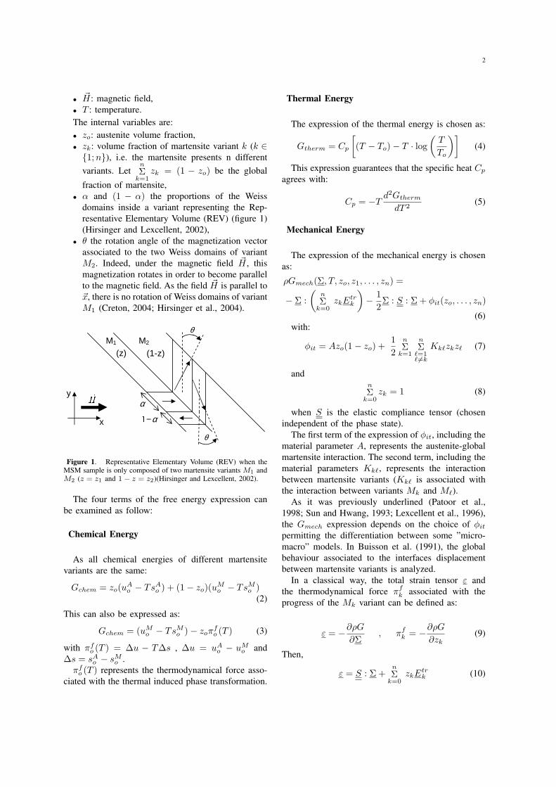
• α and (1 − α) the proportions of the Weiss

domains inside a variant representing the Rep-

resentative Elementary Volume (REV) (figure 1)

(Hirsinger and Lexcellent, 2002),

• θ the rotation angle of the magnetization vector

associated to the two Weiss domains of variant

M2. Indeed, under the magnetic field ~H , this

magnetization rotates in order to become parallel

to the magnetic field. As the field ~H is parallel to

~x, there is no rotation of Weiss domains of variant

M1 (Creton, 2004; Hirsinger et al., 2004).

M1 M2

(1-z) (z)

x

y α 1 α−

θ θ H�

Figure 1. Representative Elementary Volume (REV) when theMSM sample is only composed of two martensite variants M1 andM2 (z = z1 and 1 − z = z2)(Hirsinger and Lexcellent, 2002).

The four terms of the free energy expression can

be examined as follow:

Chemical Energy

As all chemical energies of different martensite

variants are the same:

Gchem = zo(uAo − TsA

o ) + (1 − zo)(uMo − TsM

o )(2)

This can also be expressed as:

Gchem = (uMo − TsM

o ) − zoπfo (T ) (3)

with πfo (T ) = ∆u − T∆s , ∆u = uA

o − uMo and

∆s = sAo − sM

o .

πfo (T ) represents the thermodynamical force asso-

ciated with the thermal induced phase transformation.

Thermal Energy

The expression of the thermal energy is chosen as:

Gtherm = Cp

[

(T − To) − T · log

(

T

To

)]

(4)

This expression guarantees that the specific heat Cp

agrees with:

Cp = −Td2Gtherm

dT 2(5)

Mechanical Energy

The expression of the mechanical energy is chosen

as:

ρGmech(Σ, T, zo, z1, . . . , zn) =

− Σ :

(

n

Σk=0

zkEtrk

)

− 1

2Σ : S : Σ + φit(zo, . . . , zn)

(6)

with:

φit = Azo(1 − zo) +1

2

n

Σk=1

n

Σℓ=1ℓ 6=k

Kkℓzkzℓ (7)

andn

Σk=0

zk = 1 (8)

when S is the elastic compliance tensor (chosen

independent of the phase state).

The first term of the expression of φit, including the

material parameter A, represents the austenite-global

martensite interaction. The second term, including the

material parameters Kkℓ, represents the interaction

between martensite variants (Kkℓ is associated with

the interaction between variants Mk and Mℓ).

As it was previously underlined (Patoor et al.,

1998; Sun and Hwang, 1993; Lexcellent et al., 1996),

the Gmech expression depends on the choice of φit

permitting the differentiation between some ”micro-

macro” models. In Buisson et al. (1991), the global

behaviour associated to the interfaces displacement

between martensite variants is analyzed.

In a classical way, the total strain tensor ε and

the thermodynamical force πfk associated with the

progress of the Mk variant can be defined as:

ε = −∂ρG

∂Σ, π

fk = −∂ρG

∂zk

(9)

Then,

ε = S : Σ +n

Σk=0

zkEtrk (10)

3

The left member of equation (10) corresponds to

the classical elastic strain tensor. The right member

corresponds to the phase transformation strain (be-

tween austenite and one variant of martensite) or

reorientation of martensite platelets.

πfo = Σ : Etr

o − A(1 − 2zo) (phase transformation)

(11)

πfk = Σ : Etr

k − Kkℓzℓ (k ∈ {1;n}) (reorientation)

(12)

The Clausius-Duhem inequality can be written, then

the dissipation increment is:

dD =

n∑

k=o

πfkdzk > 0 (13)

Crystallography of the Ni2MnGa

The parent austenitic phase exhibits a cubic struc-

ture called L21 (the lattice parameter ao is chosen

around 5.82 A and is considered independent of the

alloy composition and temperature). Under cooling or

stress action, this alloy can generate three different

martensitic phases:

• the modulated five-layered martensite (Quadratic

5M) with an induced strain in the order of 6 %,

• the modulated seven layered martensite structure

(Monoclinic 7M) with 10% of induced strain,

• the non modulated quadratic phase (NMT) 16 to

20%.

The present paper is devoted to the most common

Ni2MnGa martensite e.g. the 5M. This alloy was used

and a 2.5% strain up to 500 Hz was performed (Henry

et al., 2002; Marioni et al., 2003). The Ni2MnGa

MSM element applied as a sensor is investigated by

Mullner et al. (2003) and Suorsa et al. (2004).

U i describes the homogeneous deformation that

takes the lattice of the austenite to that of marten-

site and is called the ”Bain matrix” or the ”Phase

Transformation Matrix”. The austenite → martensite

5M Phase Transformation corresponds to a cubic to

tetragonal phase transformation.

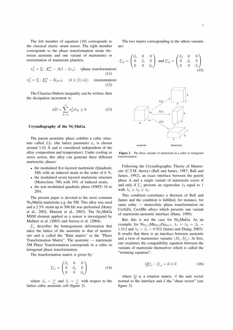
The transformation matrix is given by:

U1

=

βc 0 00 βa 00 0 βa

(14)

where βa = aao

and βc = cao

with respect to the

lattice cubic austenite cell (figure 2).

The two matrix corresponding to the others variants

are:

U2

=

βa 0 00 βc 00 0 βa

and U3

=

βa 0 00 βa 00 0 βc

(15)

ao

ao

ao (U2)

(U3)

(U1)

Austenite Martensite

c

a

a

a

c a

a

a

c

Figure 2. The three variants of martensite in a cubic to tetragonaltransformation.

Following the Crystallographic Theory of Marten-

site (C.T.M. theory) (Ball and James, 1987; Ball and

James, 1992), an exact interface between the parent

phase A and a single variant of martensite exists if

and only if U i presents an eigenvalue λ2 equal to 1

with λ1 > λ2 > λ3.

This condition constitutes a theorem of Ball and

James and the condition is fulfilled, for instance, for

same cubic → monoclinic phase transformation on

CuAlZn, CuAlBe alloys which presents one variant

of martensite-austenite interface (Hane, 1999).

But, this is not the case for Ni2MnGa. As an

example, for Ni51.3Mn24.0Ga24.7, λ1 = λ2 = βa =1.013 and λ3 = βc = 0.952 (James and Zhang, 2005).

It results that there is an interface between austenite

and a twin of martensites variants (Mi, Mj). At first,

one examines the compatibility equation between the

variants of martensite themselves which is called the

”twinning equation”:

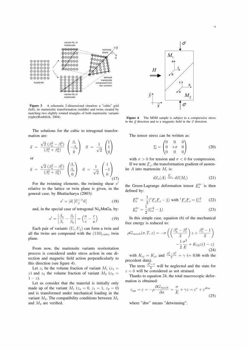
QU i − U j = ~a ⊗ ~n (16)

where Q is a rotation matrix, ~n the unit vector

normal to the interface and ~a the ”shear vector” (see

figure 3).

4

twinned martensite

composed from two variants

variant M1 of martensite

variant M2 of martensite

twinning plane

Austenite

n� a� Figure 3. A schematic 2-dimensional situation: a ”cubic” grid

(left), its martensitic transformation (middle) and twins created bymatching two slightly rotated triangles of both martensitic variants(right)(Roubıcek, 2004).

The solutions for the cubic to tetragonal transfor-

mation are:

~a =

√2 (β2

a − β2

c )

(β2c + β2

a)

βc

−βa

0

~n =1√2

110

or

~a =

√2 (β2

a − β2

c )

(β2c + β2

a)

βc

βa

0

~n =1√2

1−10

(17)

For the twinning elements, the twinning shear s′

relative to the lattice or twin plane is given, in the

general case, by Bhattacharya (2003):

s′ = |~a|∣

∣U−1

j ~n∣

∣ (18)

and, in the special case of tetragonal Ni2MnGa, by:

s′ =

∣

∣

∣

∣

βa

βc

− βc

βa

∣

∣

∣

∣

=(a

c− c

a

)

(19)

Each pair of variants (Ui, Uj) can form a twin and

all the twins are compound with the (110)cubic twin

plane.

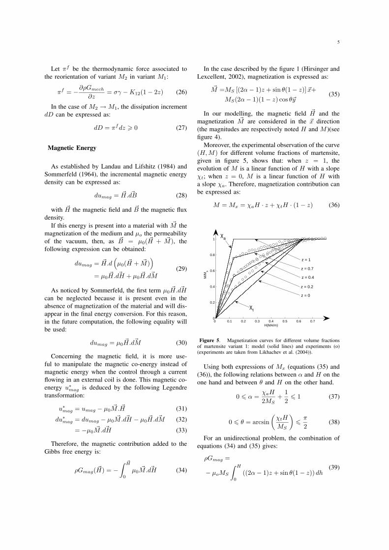
From now, the martensite variants reorientation

process is considered under stress action in one di-

rection and magnetic field action perpendicularly to

this direction (see figure 4).

Let z1 be the volume fraction of variant M1 (z1 =z) and z2 the volume fraction of variant M2 (z2 =1 − z).

Let us consider that the material is initially only

made up of the variant M1 (zo = 0, z1 = 1, z2 = 0)

and is transformed under mechanical loading in the

variant M2. The compatibility conditions between M1

and M2 are verified.

1M

2M a

a

a

a

c

c

σ σ x

� y� H

Figure 4. The MSM sample is subject to a compressive stressin the ~y direction and to a magnetic field in the ~x direction.

The tensor stress can be written as:

Σ =

0 0 00 +σ 00 0 0

(20)

with σ > 0 for tension and σ < 0 for compression.

If we note F i, the transformation gradient of austen-

ite A into martensite Mi is:

d~xo(A)F i−−→ d~x(Mi) (21)

the Green-Lagrange deformation tensor Etri is then

defined by:

Etri =

1

2(tF iF i − 1) with tF iF i = U2

i (22)

Etri =

1

2(U2

i − 1) (23)

In this simple case, equation (6) of the mechanical

free energy is reduced to:

ρGmech(σ, T, z) = −σ

((

β2

a − β2

c

2

)

z +β2

c − 1

2

)

−1

2

σ2

E+ K12z(1 − z)

(24)

with Kij = Kji andβ2

a−β2

c

2= γ (= 0.06 with the

precedent data).

The termβ2

c−1

2will be neglected and the state for

z = 0 will be considered as not strained.

Thanks to equation 24, the total macroscopic defor-

mation is obtained:

εyy = ε = −ρ∂Gmech

∂σ=

σ

E+ γz = εe + εdtw

(25)

where ”dtw” means ”detwinning”.

5

Let πf be the thermodynamic force associated to

the reorientation of variant M2 in variant M1:

πf = −∂ρGmech

∂z= σγ − K12(1 − 2z) (26)

In the case of M2 → M1, the dissipation increment

dD can be expressed as:

dD = πfdz > 0 (27)

Magnetic Energy

As established by Landau and Lifshitz (1984) and

Sommerfeld (1964), the incremental magnetic energy

density can be expressed as:

dumag = ~H. ~dB (28)

with ~H the magnetic field and ~B the magnetic flux

density.

If this energy is present into a material with ~M the

magnetization of the medium and µo the permeability

of the vacuum, then, as ~B = µ0( ~H + ~M), the

following expression can be obtained:

dumag = ~H.d(

µ0( ~H + ~M))

= µ0~H. ~dH + µ0

~H. ~dM(29)

As noticed by Sommerfeld, the first term µ0~H. ~dH

can be neglected because it is present even in the

absence of magnetization of the material and will dis-

appear in the final energy conversion. For this reason,

in the future computation, the following equality will

be used:

dumag = µ0~H. ~dM (30)

Concerning the magnetic field, it is more use-

ful to manipulate the magnetic co-energy instead of

magnetic energy when the control through a current

flowing in an external coil is done. This magnetic co-

energy u∗mag is deduced by the following Legendre

transformation:

u∗mag = umag − µ0

~M. ~H (31)

du∗mag = dumag − µ0

~M. ~dH − µ0~H. ~dM (32)

= −µ0~M. ~dH (33)

Therefore, the magnetic contribution added to the

Gibbs free energy is:

ρGmag( ~H) = −∫ ~H

0

µ0~M. ~dH (34)

In the case described by the figure 1 (Hirsinger and

Lexcellent, 2002), magnetization is expressed as:

~M =MS [(2α − 1)z + sin θ(1 − z)] ~x+

MS(2α − 1)(1 − z) cos θ~y(35)

In our modelling, the magnetic field ~H and the

magnetization ~M are considered in the ~x direction

(the magnitudes are respectively noted H and M )(see

figure 4).

Moreover, the experimental observation of the curve

(H, M) for different volume fractions of martensite,

given in figure 5, shows that: when z = 1, the

evolution of M is a linear function of H with a slope

χt; when z = 0, M is a linear function of H with

a slope χa. Therefore, magnetization contribution can

be expressed as:

M = Mx = χaH · z + χtH · (1 − z) (36)

0 0.1 0.2 0.3 0.4 0.5 0.6 0.7 0

0.2

0.4

0.6

0.8

1

H(MA/m)

M/M

s

z = 0

z = 0.2

z = 0.4

z = 0.7

z = 1

χt

χa

Figure 5. Magnetization curves for different volume fractionsof martensite variant 1: model (solid lines) and experiments (o)(experiments are taken from Likhachev et al. (2004)).

Using both expressions of Mx (equations (35) and

(36)), the following relations between α and H on the

one hand and between θ and H on the other hand.

0 6 α =χaH

2MS

+1

26 1 (37)

0 6 θ = arcsin

(

χtH

MS

)

6π

2(38)

For an unidirectional problem, the combination of

equations (34) and (35) gives:

ρGmag =

− µoMS

∫ H

0

((2α − 1)z + sin θ(1 − z)) dh(39)

6

As z and H are independent variables:

ρGmag =

− µoMS

(

z

∫ H

0

(2α − 1)dh + (1 − z)

∫ H

0

sin θdh

)

(40)

For the integration, the H domain is split in three

cases.

1) First case:

H < MS

χae.g. 0 < α < 1 , 0 < θ < π

2

⇒

∫ H

0

(2α − 1)dh =

∫ H

0

χah

MS

dh =χaH2

2MS∫ H

0

sin(θ)dh =

∫ H

0

χth

MS

dh =χtH

2

2MS

(41)

2) Second case:

MS

χa< H < MS

χte.g. α = 1 , 0 < θ < π

2

⇒

∫ H

0

(2α − 1)dh =

∫

MSχa

0

(2α − 1)dh

+

∫ H

MSχa

(2α − 1)dh = H − MS

2χa

∫ H

0

sin(θ)dh =χtH

2

2MS

(42)

3) Third case:

H > MS

χte.g. α = 1 , θ = π

2

⇒

∫ H

0

(2α − 1)dh = H − MS

2χa

∫ H

0

sin(θ)dh =

∫

MSχt

0

sin(θ)dh

+

∫ H

MSχt

sin(θ)dh = H − MS

2χt

(43)

A synthesis of the three previous cases gives:

∫ H

0

(2α − 1)dh = (2α − 1)H − MS

2χa

(2α − 1)2

∫ H

0

sin(θ)dh = sin(θ)H − MS

2χt

(sin(θ))2

(44)

Lastly, the expression of the magnetic contribution

of the Gibbs free energy function becomes:

ρGmag(H, z, α, θ) =

− µ0MS

[

z

(

(2α − 1)H − MS

2χa

(2α − 1)2)

+(1 − z)

(

sin(θ)H − MS

2χt

(sin(θ))2)]

(45)

Gibbs Free Energy Expression for Reorientation

Process of Martensite Variants

According to the previous calculations, the free

energy expression can finally be reached:

ρG(σ,H, T, z, α, θ) = Cp

[

(T − To) − T · logT

To

]

− σγz − σ2

2E+ K12z(1 − z)

− µoMS

(

z

(

(2α − 1)H − MS

2χa

(2α − 1)2)

+ (1 − z)

(

(sin θ)H − MS

2χt

(sin θ)2))

(46)

This paper deals with rearrangement of marten-

site platelets and not phase transformation explaining

why the ”chemical contribution” is not considered.

However, the magneto-mechanical expression for the

rearrangement between two variants of martensite

under magnetic field and (or) stress action is rather

complicated.

To determine G, the coupling between mechanic

and magnetism is not caused by the choice of a

magneto-mechanic Gmech,mag expression, but by the

choice of the internal variables (z in the considered

paper).

GIBBS FREE ENERGY MODEL

HANDLING

Calculations of the Different Thermodynamical

Forces

In a classical way the total deformation and the

magnetization M can be written from (25) and (35)

respectively as:

ε = −∂(ρG)

∂σ=

σ

E+ γz = εe + εdtw (47)

µoM = −∂(ρG)

∂H(48)

= µoMS ((2α − 1)z + sin θ(1 − z)) (49)

7

The thermodynamical force associated with the

progression of the Weiss domain width α and rotation

angle of the magnetization θ are:

∂(ρG)

∂α= −2µoMSz

(

H − MS

χa

(2α − 1)

)

= 0

(50)

∂(ρG)

∂θ= −µoMS(1 − z) cos θ

(

H − MS

χt

sin θ

)

= 0

(51)

The choice of the free energy expression confirms

that the pure magnetic behaviour is considered as

reversible (e.g. without hysteresis).

Finally, let us examine the thermodynamical force

associated with the z fraction of martensite:

πf∗ = −∂ρG

∂z= σγ − K12(1 − 2z)

+ µoMS

[

(2α − 1)H − MS

2χa

(2α − 1)2

−H sin θ +MS

2χt

sin2 θ

]

(52)

This can be reduced to:

πf∗ = σγ − K12(1 − 2z)

− µoM2

S

(

(1 − 2α) sin θ

χt

+(2α − 1)2

2χa

+sin2 θ

2χt

)

(53)

The mechanical behaviour of the considered mate-

rial is highly irreversible e.g. with strong hysteresis.

Hence the inequality of Clausius-Duhem can be writ-

ten as:

dD = −ρdG(σ,H, T, z) − µoMdH − εdσ > 0(54)

This expression can be reduced to:

dD = πf∗dz > 0 (55)

Kinetic Equations and Minor Loops

To obtain the full characterization of the thermo-

dynamic behaviour, the previous set of equations has

to be completed with kinetic equations. The complete

forward and reverse transformations (major loop) can

so be obtained.

Let us note the equation (53) as:

πf∗ = Π(σ, α, θ) − K12(1 − 2z) (56)

with:

Π(σ, α, θ) = σγ − µoM2

S

(

(1 − 2α) sin θ

χt

+(2α − 1)2

2χa

+sin2 θ

2χt

) (57)

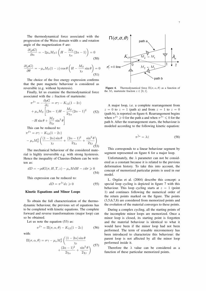
z ( , , )σ α θΠ 0 12K * 0fπ =

oλ path a

path b

1 2 1M M→2 1M M← line Figure 6. Thermodynamical force Π(σ, α, θ) as a function of

the M1 martensite fraction z ∈ [0, 1].

A major loop, i.e. a complete rearrangement from

z = 0 to z = 1 (path a) and from z = 1 to z = 0(path b), is reported on figure 6. Rearrangement begins

when πf∗ > 0 for the path a and when πf∗ 6 0 for the

path b. After the rearrangement starts, the behaviour is

modeled according to the following kinetic equation:

˙πf∗ = λz (58)

This corresponds to a linear behaviour segment by

segment represented on figure 6 for a major loop.

Unfortunately, the λ parameter can not be consid-

ered as a constant because it is related to the previous

deformation history. To take this into account, the

concept of memorized particular points is used in our

model.

L. Orgeas et al. (2004) describe this concept: a

special loop cycling is depicted in figure 7 with this

behaviour. This loop cycling starts at z = 1 (point

1) and continues following the numerical order of

the return points marked on the figure. The points

(3,5,6,7,8) are considered from memorized points and

the evolution of the material converges to these points.

During a complex cycling, all the starting points of

the incomplete minor loops are memorized. Once a

minor loop is closed, its starting point is forgotten

and the material behaviour is identical to what it

would have been if the minor loop had not been

performed. The term of erasable micromemory has

been introduced to characterize this behaviour: the

parent loop is not affected by all the minor loop

performed inside it.

Therefore the λ value can be considered as a

function of these particular memorized points.

8 z ( , , )σ α θΠ 1 � � � � � � � � 0

Figure 7. Description of a special loop cycling including theconcept of memorized particular points.

Heat Equation

Furthermore, the heat equation can be expressed

from the Gibbs free energy expression. The energy

conservation principle induces the following equation:

ρu(ε, ~M, s, z, α, θ) = −pi + rext − div~q (59)

where pi = −Σ : ε − µ0~H · ~M is the power of

internal effort, rext is the external heat contribution

and ~q is the heat flux density vector.

According to the Legendre transformation:

G(Σ, ~H, T, z, α, θ) =

u(ε, ~M, s, z, α, θ) − Ts − σ : ε

ρ− µ0

~H · ~M

ρ

(60)

We can obtain:

ρG = rext − div~q − ρT s − ρsT

−σ : ε − µ0~H · ~M

(61)

On the other hand:

ρG =∂ρG

∂σσ +

∂ρG

∂HH +

∂ρG

∂TT +

∂ρG

∂zz

+∂ρG

∂αα +

∂ρG

∂θθ

= −εσ − µ0MH − ρsT − πf∗z + 0 · α + 0 · θ(62)

The combination of equations (61) and (62) gives:

πf∗z = −rext + div~q + ρT s (63)

By introducing the Cp parameter, the heat equation

expression is finally written:

πf∗z = −rext + div~q + ρCpT (64)

COMPARAISON BETWEEN MODEL

PREDICTION AND EXPERIMENTS

Experimental Set-up

The MSM sample which is used comes from Adap-

tamat Ltd. Its dimensions are 3 × 5 × 20 mm. The

martensite start temperature of the material is 36◦C.

Experiments are achieved at room temperature. A

magnetic field is created by a coil and concentrated

by a ferromagnetic circuit into an horizontal air-

gap. Mechanical loading can be applied vertically

(perpendicular to the magnetic field) with masses and

a lever arm. A F.W. Bell 7010 teslameter enables to

measure the magnetic field into the air-gap and a LAS

2010V laser sensor displays a vertical displacement

information.

Equivalence Between Magnetic Field H and

Stress Action σ: Yield Line (H, σ) for Martensite

Variants Rearrangement Initiation

In a classical way, the rearrangement process starts

when the thermodynamical force πf∗ reaches a critical

value called πcr. For a constant temperature T < A0

s:

πf∗(σ,H, z = 0) = πcr (65)

⇒πcr = σγ − K12

− µoM2

S

(

(1 − 2α) sin θ

χt

+(2α − 1)2

2χa

+sin2 θ

2χt

)

(66)

Three situations must be examined.

• Zone I: no saturation appears in α and θ.

By using the following relations between α and

H on one part and between θ and H on an

another part:

2α − 1 =χaH

MS

(67)

sin θ =χtH

MS

(68)

Finally, the critical thermodynamical force is:

πcr = σγ − K12 −µ0H

2

2(χt − χa) (69)

σ is affine in the square of H .

• Zone II: saturation appears in α but not in θ.

9

α = 1 , sin θ = χtHMS

πcr = σγ − K12 −µ0M

2

S

2χa

+ µoMSH − µ0χt

2H2

(70)

σ is affine in a second degree polynom in H .

• Zone III: saturation appears in α and θ.

α = 1 and sin θ = 1

πcr = σγ − K12 −µ0M

2

S

2

(

1

χa

− 1

χt

)

(71)

In this third situation σ reaches a constant value

whatever H .

Figure 8 enables to compare experimental measure-

ments to predictions with:

µ0MS = 0.65 T , χt = 0.82 , χa = 4 , πcr+K12 =20.103 Pa , γ = 0.055

−4 −3.5 −3 −2.5 −2 −1.5 −1 −0.5 0 0.5 0

0.1

0.2

0.3

0.4

0.5

0.6

σ (MPa)

H (

MA

/m)

M2

M1

Zone I

Zone II

Zone III

Figure 8. Yield line (H, σ) for martensite variants rearrangementinitiation - model prediction (line) and experiments (points).

Mechanical Testing With or Without Magnetic

Field

For these experiments, according to the hypothesis

of the model, z = 0 and ε = 0 correspond to a sample

composed of only M2 variant (first situation). z = 1and ε = γ correspond to a sample composed of only

M1 variant (second situation). The starting point of

these experiments corresponds to the second situation

(z = 1). A compressive stress is applied to transform

the M1 variant into the M2 variant then released (σ =0 → σ = −|σmax| → σ = 0).

The first experiment is conducted without magnetic

field and the second one is conducted when a constant

magnetic field is applied (H = 600 kA/m). The

parameters for the model are the same than before

−2 −1 0 1 2 3 4 5−8

−6

−4

−2

0

ε (%)

σ (M

Pa)

−2 −1 0 1 2 3 4 5−8

−6

−4

−2

0

ε (%)

σ (M

Pa)

H = 0 A/m

H = 600 kA/m

Finishing point(z = 0,M

2)

Starting point(z = 1,M

1)

Starting and finishing points(z = 1,M

1)

(z = 0,M2)

Figure 9. Strain vs stress plots for two different magnetic fields:model prediction (solid line) and experiments (crosses or circles).

with moreover: πcr = 0, λ0 = 110.103 Pa and

E = 500.106 Pa. The results are reported on the figure

9.

The first experiment enables to note that the fin-

ishing point does not correspond to the starting point

whereas these two points correspond when the mag-

netic field is applied. The antagonistic effect be-

tween compressive stress and magnetic field is clearly

demonstrated: the forward deformation is obtained by

the stress when the backward deformation is recov-

ered by the magnetic field. Moreover the predictions

correspond well to the measurements.

Tests Under Constant Compressive Load

The starting point of this experiment corresponds

to the first situation described above (z = 0, ε = 0).

Then, a mass is applied to exert a constant compres-

sive load σ (z = 0, ε = εe). By means of an electro-

magnet, a magnetic field is applied: two identical

cycles (H = 0 → H = Hmax → H = 0) are

repeated. This enables to show first an external loop

and secondly an internal loop.

10

0 0.2 0.4

0246

σ = 0 MPa

H(MA/m)

ε (%

)

0 0.2 0.4

0246

σ = −0.25 MPa

H(MA/m)

ε (%

)0 0.2 0.4

0246

σ = −0.5 MPa

H(MA/m)

ε (%

)

0 0.2 0.40246

σ = −0.75 MPa

H(MA/m)

ε (%

)

0 0.2 0.40246

σ = −1 MPa

H(MA/m)

ε (%

)

0 0.2 0.40246

σ = −1.25 MPa

H(MA/m)

ε (%

)

0 0.2 0.40246

σ = −1.5 MPa

H(MA/m)

ε (%

)

0 0.2 0.40246

σ = −1.75 MPa

H(MA/m)

ε (%

)

0 0.2 0.4

0246

σ = −2 MPa

H(MA/m)

ε (%

)

0 0.2 0.4

0246

σ = −2.25 MPa

H(MA/m)

ε (%

) Figure 10. Strain vs magnetic field plots for different stresses:model prediction (dotted line) and experiments (solid line).

11

This experiment is conducted for different masses

(σ = 0 , −0.25, −0.5, −0.75, −1, −1.25, −1.5,

−1.75, −2 and −2.25 MPa) and its results are re-

ported on the figure 10.

We can notice some discrepancy between prediction

and measurements, but, the model predicts relatively

well the external and the internal loop. For this large

pre-stress bandwidth, the results of the model are quite

encouraging.

CONCLUSION

A new model integrating uniaxial stress action per-

pendicular to the magnetic field on a MSM Ni2MnGa

single crystal is built. The material behaviour is con-

sidered as magnetically reversible and mechanically

irreversible. Thanks to the thermodynamical force

associated to the martensite reorientation initiation

process, an equivalence between magnetic field H and

stress action σ is obtained. The curves describing the

strain evolution ε as a function of magnetic field H ,

under constant external compression, are fairly fitted

by the present model. Future works will concern the

design and control of actuators using MSMs as active

elements in a smart structure.

NOMENCLATURE

Mi = martensite variant iG = Gibbs free energy

Gchem = chemical Gibbs free energyGmech = mechanical Gibbs free energyGmag = magnetic Gibbs free energy

Gtherm = thermal Gibbs free energyΣ = applied stress tensorT = temperature~H = magnetic fieldzo = austenite volume fraction

1 − zo = martensite volume fractionzk = volume fraction of martensite variant kn = number of different variantsα = proportion of the Weiss domain inside a variantθ = rotation angle of the magnetization vector~M = magnetization vector

uAo = specific internal energy of the austenite phase

uMo = specific internal energy of the martensite phase

sAo = specific entropy of the austenite phase

sMo = specific entropy of the martensite phaseTo = reference temperatureCp = specific heat

Etrk = rearrangement deformation tensorS = elastic compliance tensor

A = interaction parameter between austenite and martensiteKkl = interaction parameter between Mk and Ml

ao = lattice parameter of austenite phaseU i = phase transformation matrix from austenite into Mi

a = long lattice parameter of martensite phasec = short lattice parameter of martensite phase

βa = aao

βc = cao

Q = rotation matrix~n = unit normal to the interface~a = ”shear vector”s′ = twinning shearz = z1 for the simple case (M1 fraction)

1 − z = z2 for the simple case (M2 fraction)σ = applied stress for the simple case

M = magnetization for the simple caseH = magnetic field for the simple caseε = total strain for the simple case

εe = elastic strain for the simple case

εdtw = ”detwinning” strain for the simple caseF i = transformation gradient tensor of austenite into Mi

E = Young’s modulusγ = total uniaxial rearrangement strainρ = mass density

umag = magnetic energy~B = magnetic flux density

u∗

mag = magnetic co-energy

µo = permeability of the vacuumMS = saturation magnetizationχt = magnetic susceptibility for hard magnetization directionχa = magnetic susceptibility for easy magnetization directionAo

s = austenite start temperature at stress free state

πf∗ = thermodynamical force associated with zdD = dissipation increment

λ = kinetic parameterλo = kinetic parameter for major loopu = specific internal energypi = power of internal effort

rext = external heat source~q = heat flux density vectors = specific entropy

πcr = critical value for thermodynamical force πf∗

REFERENCES

Ball, J. and James, R. 1987. “Fine phase mixtures asminimizers of energy”. Arch. Rational. Mech. Anal.,100:13–52.

Ball, J. and James, R. 1992. “Proposed experimental testsof the theory of fine microstructure and the two wellproblem”. Phil. Trans. Royal Soc. London, A 338:389–450.

Bhattacharya, K. 2003. Microstructure of Martensite : WhyIt Forms and How It Gives Rise to the Shape-MemoryEffect. Oxford series on materials modelling.

Buisson, M., Patoor, E., and Berveiller, M. 1991. “Com-portement global associe aux mouvements d’interfacesentre variantes de martensite”. C.R. Acad. Sci. Paris,313(2):587–590.

Creton, N. 2004. Etude du comportement magneto-mecanique des alliages a memoire de forme de typeHeusler Ni-Mn-Ga. PhD thesis, Universite de Franche-Comte (France).

Hane, K. F. 1999. “Bulk and thin film microstructures inuntwinned martensites”. Journal of the Mechanics andPhysics of Solids, 47(9):1917–1939.

Henry, C., Bono, D., Feuchtwanger, J., Allen, S., andO’Handley, R. 2002. “Field-induced actuation ofsingle crystal ni-mn-ga”. J. of Applied Phys., 91:7810–7811.

Hirsinger, L., Creton, N., and Lexcellent, C. 2004. “Fromcrystallographic properties to macroscopic detwinningstrain and magnetisation of ni-mn-ga magnetic shapememory alloys”. J. Phys. IV, 115:111–120.

12

Hirsinger, L. and Lexcellent, C. 2002. “Modelling detwin-ning of martensite platelets under magnetic and (or)stress actions in ni-mn-ga alloys”. J. of Magnetismand Magnetic Materials, 254-255:275–277.

James, R. and Zhang, Z. 2005. “A way to search formultiferroic materials with ”unlikely” combinationsof physical properties”. to appear in ”Interplay ofMagnetism and Structure in Functional Materials”(ed. L. Manosa, A. Planes, A.B. Saxena), SpringerVerlag.

Landau, L., Lifshitz, E., and Pitaevskii, L. 1984. Electro-dynamics of Continuous Media : Volume 8 (Courseof Theoretical Physics) (2nd Edition). Butterworth-Heinemann.

Lexcellent, C., Goo, B., Sun, Q., and Bernardini, J.1996. “Characterization, thermodynamical behav-iour and micromechanical-based constitutive model ofshape memory cu-zn-al single crystals”. Acta. Met.Mat., 44(9):3773–3780.

Likhachev, A., Sozinov, A., and Ullakko, K. 2004. “Dif-ferent modeling concepts of magnetic shape memoryand their comparison with some experimental resultsobtained in ni-mn-ga”. Materials Science and Engi-neering A, 378:513–518.

Marioni, M., O’Handley, R., and Allen, S. 2003. “Pulsedmagnetic field-induced actuation of ni-mn-ga singlecrystals”. Applied Physics Letters, 83:3966–3968.

Mori, T. and Tanaka, K. 1973. “Average stress in matrixand average elastic energy of materials with misfittinginclusions”. Acta Met., 21:571–574.

Mullner, P., Chernenko, V., and Kostorz, G. 2003. “Stress-induced twin rearrangement resulting in change ofmagnetization in a ni-mn-ga ferromagnetic marten-site”. Scripta Mat., 49:129–133.

Orgeas, L., Vivet, A., Favier, D., Lexcellent, C., and Liu,Y. 2004. “Hysteretic behaviour of a cu-zn-al singlecrystal during superelastic shear deformation”. ScriptaMaterialia, 51:297–302.

Patoor, E., Eberhardt, A., and Berveiller, M. 1998. “Thermo-mechanical modelling of shape memory alloys”. Arch.Mech., 40-5,6:775–794.

Roubıcek, T. 2004. “Models of microstructure evolution inshape memory alloys”. In Nonlinear Homogenizationand its Applications to Composites, Polycrystals andSmart Materials, pages 269–304. P. Ponte Castanedaet al. eds., Kluwer.

Sommerfeld, A. 1964. Thermodynamics and StatisticalMechanics. Academic Press.

Sun, Q. and Hwang, K. 1993. “Micromechanics modellingfor the constitutive behavior of polycrystalline shapememory alloys - i : Derivation of general relations”.J. Mech. Phys. Solids, 41(1):1–17.

Suorsa, I., Tellinen, J., Aaltio, I., Pagounis, E., and Ullakko,K. 2004. “Design of active element for msm-actuator”.In ACTUATOR 2004 / 9th International Conference onNew Actuators, Bremen (Germany).