J. Agr. Sci. Tech. (2017) Vol. 19: 1439-1452

1439

1 Department of Agricultural Economics, Extension and Rural Development, University of Pretoria, South

Africa. * Corresponding author; email: mesay44@gmail.com 2 Bureau for Food and Agricultural Policy (BFAP), University of Pretoria, South Africa. 3 Centre for Environmental Economics and Policy Analysis (CEEPA), University of Pretoria, South

Africa.

Modelling Price Formation and Dynamics in the Ethiopian

Maize Market

M. Y. Gurmu1*, F. Meyer2, and R. Hassan3

ABSTRACT

This study is an attempt to examine price formation, and dynamics in the Ethiopian

maize market. A single commodity partial equilibrium and the Johansen’s co-integration

approaches were used to investigate maize price formation and market integration in the

Ethiopian maize market. Findings from the maize industry outlook indicated that maize

production is expected to grow for the forecasted period. An increase in maize production

was, however, not enough to offset the growth on the demand side. From the yield

simulation analysis, we found that a 20% increase in maize yield would reduce nominal

maize price by 81%. Co-integration analysis indicated that the Ethiopian wholesale maize

markets have become more efficient in the recent years suggesting that price related

information is transmitted more efficiently across consumption and production wholesale

maize markets.

Keywords: Agricultural market, Equilibrium price, Maize, Market integration, Price

formation.

INTRODUCTION

With the recent turmoil in international food

market, “getting market prices right” has

become an important topic for most

governments, including the Ethiopian

government. In response to the sharp rise in

domestic grain prices of 2007/2008, the

Ethiopian government introduced a wide range

of policy instruments to tame the soaring

domestic food prices. After the reform of

market liberalization in March 1990, for the

first time the government has become heavily

involved in commercial wheat imports. As a

form of domestic supply stabilization policy,

the Ethiopian government additionally

imposed an indefinite export ban on major

cereal crops including maize, sorghum, teff

and wheat. Generally, it is argued that before

embarking on any intervention in domestic

grain market, a better understanding of the

price formation and possible scenarios of the

dynamic grain market environment is crucial

for policy makers to make informed decisions

for the betterment of producers, investors,

traders, and consumers’ welfare. Moreover,

the dynamic market environment in which

producers and consumers operate necessitate a

better understanding of price discovery and

dynamics of the product they produce. It is

against this backdrop that commodity

modelling can provide valuable information to

assist role players in decision-making.

Several studies have attempted to analyse

inter-regional spatial grain market integration

in Ethiopia (Negassa et al., 2004; Getnet et al.,

2005; Jaleta and Gebremedhin, 2009;

Ulimwengu et al. 2009; Kelbore, 2013;

Tamru, 2013). These studies used different

approaches ranging from the primitive

correlation analysis to dynamic time series

Dow

nloa

ded

from

jast

.mod

ares

.ac.

ir at

8:0

7 IR

ST

on

Sun

day

Janu

ary

9th

2022

_______________________________________________________________________ Gurmu et al.

1440

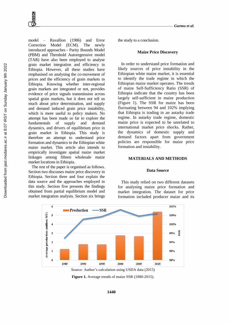
Source: Author’s calculation using USDA data (2015)

Figure 1. Average trends of maize SSR (1980-2015).

model – Ravallion (1986) and Error

Correction Model (ECM). The newly

introduced approaches - Parity Bounds Model

(PBM) and Threshold Autoregressive model

(TAR) have also been employed to analyse

grain market integration and efficiency in

Ethiopia. However, all these studies have

emphasised on analysing the co-movement of

prices and the efficiency of grain markets in

Ethiopia. Knowing whether inter-regional

grain markets are integrated or not, provides

evidence of price signals transmission across

spatial grain markets, but it does not tell us

much about price determination, and supply

and demand induced grain price instability,

which is more useful to policy makers. No

attempt has been made so far to explore the

fundamentals of supply and demand

dynamics, and drivers of equilibrium price in

grain market in Ethiopia. This study is

therefore an attempt to understand price

formation and dynamics in the Ethiopian white

maize market. This article also intends to

empirically investigate spatial maize market

linkages among fifteen wholesale maize

market locations in Ethiopia.

The rest of the paper is organised as follows.

Section two discusses maize price discovery in

Ethiopia. Section three and four explain the

data source and the approaches employed in

this study. Section five presents the findings

obtained from partial equilibrium model and

market integration analysis. Section six brings

the study to a conclusion.

Maize Price Discovery

In order to understand price formation and

likely sources of price instability in the

Ethiopian white maize market, it is essential

to identify the trade regime in which the

Ethiopian maize market operates. The trends

of maize Self-Sufficiency Ratio (SSR) of

Ethiopia indicate that the country has been

largely self-sufficient in maize production

(Figure 1). The SSR for maize has been

fluctuating between 94 and 102% implying

that Ethiopia is trading in an autarky trade

regime. In autarky trade regime, domestic

maize price is expected to be unrelated to

international market price shocks. Rather,

the dynamics of domestic supply and

demand factors apart from government

policies are responsible for maize price

formation and instability.

MATERIALS AND METHODS

Data Source

This study relied on two different datasets

for analysing maize price formation and

market integration. The dataset for price

formation included producer maize and its Dow

nloa

ded

from

jast

.mod

ares

.ac.

ir at

8:0

7 IR

ST

on

Sun

day

Janu

ary

9th

2022

Maize Price Formation and Dynamics __________________________________________

1441

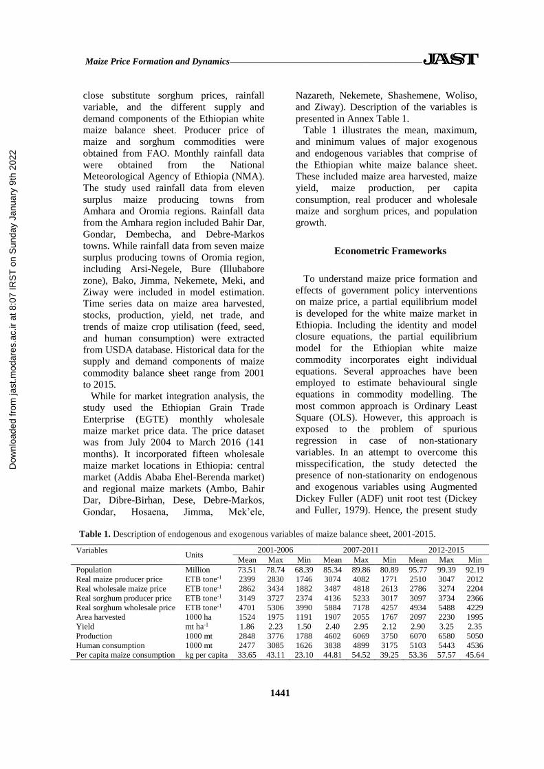
Table 1. Description of endogenous and exogenous variables of maize balance sheet, 2001-2015.

Variables

Units

2001-2006 2007-2011 2012-2015

Mean Max Min Mean Max Min Mean Max Min

Population Million 73.51 78.74 68.39 85.34 89.86 80.89 95.77 99.39 92.19

Real maize producer price ETB tone-1 2399 2830 1746 3074 4082 1771 2510 3047 2012

Real wholesale maize price ETB tone-1 2862 3434 1882 3487 4818 2613 2786 3274 2204

Real sorghum producer price ETB tone-1 3149 3727 2374 4136 5233 3017 3097 3734 2366

Real sorghum wholesale price ETB tone-1 4701 5306 3990 5884 7178 4257 4934 5488 4229

Area harvested 1000 ha 1524 1975 1191 1907 2055 1767 2097 2230 1995

Yield mt ha-1 1.86 2.23 1.50 2.40 2.95 2.12 2.90 3.25 2.35

Production 1000 mt 2848 3776 1788 4602 6069 3750 6070 6580 5050

Human consumption 1000 mt 2477 3085 1626 3838 4899 3175 5103 5443 4536

Per capita maize consumption kg per capita 33.65 43.11 23.10 44.81 54.52 39.25 53.36 57.57 45.64

close substitute sorghum prices, rainfall

variable, and the different supply and

demand components of the Ethiopian white

maize balance sheet. Producer price of

maize and sorghum commodities were

obtained from FAO. Monthly rainfall data

were obtained from the National

Meteorological Agency of Ethiopia (NMA).

The study used rainfall data from eleven

surplus maize producing towns from

Amhara and Oromia regions. Rainfall data

from the Amhara region included Bahir Dar,

Gondar, Dembecha, and Debre-Markos

towns. While rainfall data from seven maize

surplus producing towns of Oromia region,

including Arsi-Negele, Bure (Illubabore

zone), Bako, Jimma, Nekemete, Meki, and

Ziway were included in model estimation.

Time series data on maize area harvested,

stocks, production, yield, net trade, and

trends of maize crop utilisation (feed, seed,

and human consumption) were extracted

from USDA database. Historical data for the

supply and demand components of maize

commodity balance sheet range from 2001

to 2015.

While for market integration analysis, the

study used the Ethiopian Grain Trade

Enterprise (EGTE) monthly wholesale

maize market price data. The price dataset

was from July 2004 to March 2016 (141

months). It incorporated fifteen wholesale

maize market locations in Ethiopia: central

market (Addis Ababa Ehel-Berenda market)

and regional maize markets (Ambo, Bahir

Dar, Dibre-Birhan, Dese, Debre-Markos,

Gondar, Hosaena, Jimma, Mek’ele,

Nazareth, Nekemete, Shashemene, Woliso,

and Ziway). Description of the variables is

presented in Annex Table 1.

Table 1 illustrates the mean, maximum,

and minimum values of major exogenous

and endogenous variables that comprise of

the Ethiopian white maize balance sheet.

These included maize area harvested, maize

yield, maize production, per capita

consumption, real producer and wholesale

maize and sorghum prices, and population

growth.

Econometric Frameworks

To understand maize price formation and

effects of government policy interventions

on maize price, a partial equilibrium model

is developed for the white maize market in

Ethiopia. Including the identity and model

closure equations, the partial equilibrium

model for the Ethiopian white maize

commodity incorporates eight individual

equations. Several approaches have been

employed to estimate behavioural single

equations in commodity modelling. The

most common approach is Ordinary Least

Square (OLS). However, this approach is

exposed to the problem of spurious

regression in case of non-stationary

variables. In an attempt to overcome this

misspecification, the study detected the

presence of non-stationarity on endogenous

and exogenous variables using Augmented

Dickey Fuller (ADF) unit root test (Dickey

and Fuller, 1979). Hence, the present study

Dow

nloa

ded

from

jast

.mod

ares

.ac.

ir at

8:0

7 IR

ST

on

Sun

day

Janu

ary

9th

2022

_______________________________________________________________________ Gurmu et al.

1442

estimated behavioural equations using a

combination of the Error Correction Model

(ECM) (for non-stationary & co-integrated

series) and OLS (for stationary equations).

Maize area harvested and ending stocks

equations were estimated using Error

Correction Model (ECM). Whereas, maize

yield and per capita maize consumption

equations were estimated using OLS.

After estimating the single behavioural

equations, the next step was to estimate the

model closure. The choice of closure

technique depends on the trade regimes. As

illustrated in Figure 1, model closure under

autarky trade regime is determined by

equating total supply and total demand.

Price is thus solved endogenously in the

domestic market. Once the behavioural

equations are estimated, it is important to

make sure that the results are capturing a

true reflection of the maize market decision-

making behaviour in Ethiopia. One way of

checking robustness of model estimation is

through model validation techniques.

Following Pindyck and Rubinfeld (1991),

the following seven statistical techniques

namely Mean Average Error (MAE), Mean

Average Percentage Error (MAPE), Root

Mean Squared Error (RMSE), Theil

Inequality Coefficient (U), Bias, Variance,

and Covariance proportions were employed

to evaluate the forecasting ability of the

model.

In addition, this study examined spatial

maize market integration among fifteen

wholesale maize market locations in

Ethiopia. Given the small sample properties

and multivariate nature, the Johansen’s

Maximum Likelihood (ML) method was

used to test maize market integration. To

illustrate the model specification steps for

the Johansen’s ML method, suppose that a

set of g wholesale maize market prices (g ≥ 2) are under consideration that are I(1) and

co-integrated.

A VAR with k lags containing these

variables could be set up:

𝑦𝑡= 𝛽1𝛾𝑡−1 + 𝛽2𝛾𝑡−2 + ⋯ + 𝛽𝑘𝛾𝑡−𝑘 + 𝑢𝑡 (1)

A Vector Error Correction Model (VECM)

of the above VAR (1) form can be specified

as follows:

Δ𝑦𝑡 = Π 𝛾𝑡−𝑘+ Γ1Δ 𝛾𝑡−1+ Γ2Δ 𝛾𝑡−2 +…

Γ𝑘−1Δ 𝛾𝑡−(𝑘−1) + 𝑢𝑡 (2)

where Π = (∑ 𝛽𝑖𝑘𝑖=1 ) − 𝐼𝑔 and Γ𝑖 =

(∑ 𝛽𝑗𝑖𝑗=1 ) − 𝐼𝑔

The test for co-integration between the

‘y’s is calculated by looking at the rank of

the Π matrix. The rank of the Π matrix is

equal to the number of non-zero

characteristic roots or Eigen values. The

Eigen values denoted by 𝜆𝑖 must be positive

and less than one in absolute value and are

put in ascending order 𝜆𝑖 ≥ 𝜆2 ≥ ⋯ ≥ 𝜆𝑔. If the variables are not co-integrated,

the rank of Π will not be significantly

different from zero, so 𝜆𝑖 ≈ 0 ∀ 𝑖. Trace

and Max-Eigen test statistics were used to

test for the presence of co-integration under

the Johansen approach. The test statistics are

formulated as:

𝜆𝑡𝑟𝑎𝑐𝑒 (𝑟) = −𝑇 ∑ ln (1 −𝑔𝑖=𝑟+1 𝜆�̂�),

and (3)

𝜆𝑚𝑎𝑥 (𝑟, 𝑟 + 1) = −𝑇 ln(1 − �̂� r +1) (4)

where, 𝑟 is the number of co-integrating

vectors under the null hypothesis and 𝜆�̂� is

the estimated value for the ith ordered Eigen

value from the matrix. The test statistics

follow non-standard distribution, and the

critical values are provided by Johansen and

Juselius (1990). If the test statistic is greater

than the critical value obtained from the

Johansen’s table, reject the null of r co-

integrating vectors in favour of the

alternative 𝑟 + 1 (𝜆𝑚𝑎𝑥) or more than 𝑟 for

(𝜆𝑡𝑟𝑎𝑐𝑒). The testing is conduced

sequentially under the null, 𝑟 =0, 1, … . , 𝑔 − 1 (Brooks, 2008).

For 1< rank (Π) <g, there are r co-

integrating vectors. Π is then defined as the

product of the two matrices, 𝛼 and 𝛽, of

dimension (g × r) and (r × g), respectively.

i.e.

Π= 𝛼𝛽′ (5)

Dow

nloa

ded

from

jast

.mod

ares

.ac.

ir at

8:0

7 IR

ST

on

Sun

day

Janu

ary

9th

2022

Maize Price Formation and Dynamics __________________________________________

1443

Table 2. Results for maize supply response.

Variables Coefficient Std Error

Short-run elasticities

Constant 0.043** 0.016

D(RPMAIZEP) 0.062 0.174

D(RPSORGP) -0.057 0.199

D(RAINL) 0.0004** 0.0002

Error (-1) -0.205 0.115

Adjusted R2 0.59

F-statistics 2.87*

Long-run supply response

Constant 897.74 521.87

RPMAIZEP 0.167 0.329

RPSORGP -0.139 0.268

LNTREND 65.061** 16.662

RAINL 1.128 1.006

Adjusted R2 0.52

F-statistics 4.750**

*, **: Stand for significance at 10 and 5% levels.

The matrix 𝛽 gives the co-integrating

vectors, while 𝛼 is known as the adjustment

parameters.

RESULTS AND DISCUSSION

Modelling Maize Price Formation

Area Harvested

Table 2 summarizes the results obtained

from the dynamic error correction model by

regressing maize acreage on deflated own

and substitute crop prices, time trend and

rainfall for maize area for the period 2001-

2015. Area harvested, sorghum and maize

real producer prices were converted to

logarithmic value in order to easily interpret

values as elasticities.

Estimating the maize supply response using

adaptive expectation and partial adjustment

models would lead to spurious regression.

Alemu et al. (2003) have pointed out that

spurious regression and inconsistent and

indistinct short-run and long-run elasticity

estimates are the major pitfalls of the

traditional Nerlovian supply response

models. We have made an attempt to

estimate a maize acreage model using an

Error Correction Model (ECM). ECM

overcomes spurious regression problems and

give robust estimates of short-run and long-

run elasticities.

We modelled the maize supply response

equation using the two-stage approaches

proposed by Alemu et al. (2003). First, a

static long-run equilibrium regression is

estimated. Second, a dynamic error

correction model is conducted by including

the lagged residual from the static long-run

equilibrium regression (of course, the

residual from long-run equilibrium

regression should be stationary). Findings

from the maize supply response suggest that

farmers respond very little to price in

planning their maize acreage. The estimates

of low short-run and long-run price

elasticities of supply are comparable with

the results that have been obtained by other

studies in the field of supply response in

Ethiopia and elsewhere in smallholder

farmers’ responsiveness to market incentives

(Alemu et al., 2003; Tripathi, 2008). The

low price elasticities of supply can be

attributed to structural constraints that have

limited farmers in making informed

adjustment to market incentives. The land

tenure system also contributes to the low

magnitude of agricultural supply response in

Ethiopia. In Ethiopia, land belongs to the

state and farmers cannot lease it or get it

from other farmers. As a result, farmers

continue to practice farming within their

small landholding sizes, with little or no

prospects for acquiring additional land or for

expanding their cultivation. The other reason

for low supply response is the subsistence

nature of maize farming practices in

Ethiopia. Maize is mainly produced for

household consumption (> 75%). Only 13%

of maize production is marketed (CSA,

2011).

Furthermore, we also noticed that non-

price factors such as rainfall and

technological progress captured by the trend

variable are more important determinants in

the maize supply response than price-related

factors are. Hence, from this analysis, it can

Dow

nloa

ded

from

jast

.mod

ares

.ac.

ir at

8:0

7 IR

ST

on

Sun

day

Janu

ary

9th

2022

_______________________________________________________________________ Gurmu et al.

1444

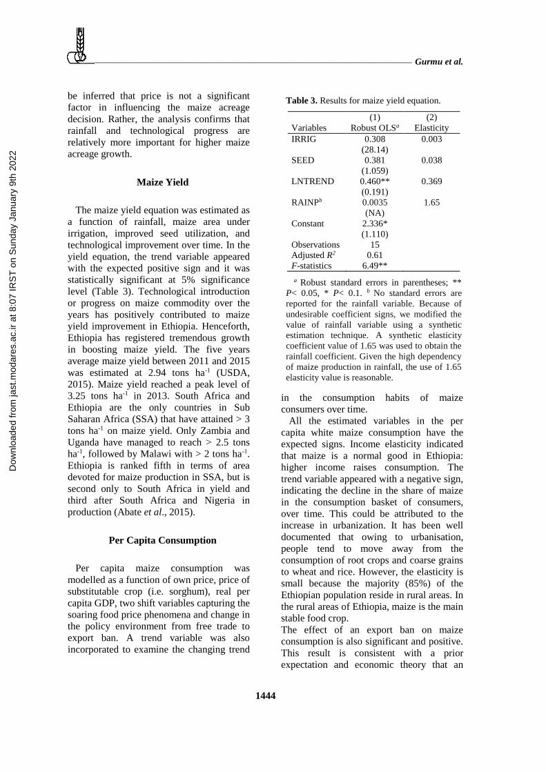
Table 3. Results for maize yield equation.

(1) (2)

Variables Robust OLSa Elasticity

IRRIG 0.308 0.003

(28.14)

SEED 0.381 0.038

(1.059)

LNTREND 0.460** 0.369

(0.191)

RAINPb 0.0035 1.65

(NA)

Constant 2.336*

(1.110)

Observations 15

Adjusted R2

F-statistics

0.61

6.49**

a Robust standard errors in parentheses; **

P< 0.05, * P< 0.1. b No standard errors are

reported for the rainfall variable. Because of

undesirable coefficient signs, we modified the

value of rainfall variable using a synthetic

estimation technique. A synthetic elasticity

coefficient value of 1.65 was used to obtain the

rainfall coefficient. Given the high dependency

of maize production in rainfall, the use of 1.65

elasticity value is reasonable.

be inferred that price is not a significant

factor in influencing the maize acreage

decision. Rather, the analysis confirms that

rainfall and technological progress are

relatively more important for higher maize

acreage growth.

Maize Yield

The maize yield equation was estimated as

a function of rainfall, maize area under

irrigation, improved seed utilization, and

technological improvement over time. In the

yield equation, the trend variable appeared

with the expected positive sign and it was

statistically significant at 5% significance

level (Table 3). Technological introduction

or progress on maize commodity over the

years has positively contributed to maize

yield improvement in Ethiopia. Henceforth,

Ethiopia has registered tremendous growth

in boosting maize yield. The five years

average maize yield between 2011 and 2015

was estimated at 2.94 tons ha-1 (USDA,

2015). Maize yield reached a peak level of

3.25 tons ha-1 in 2013. South Africa and

Ethiopia are the only countries in Sub

Saharan Africa (SSA) that have attained > 3

tons ha-1 on maize yield. Only Zambia and

Uganda have managed to reach > 2.5 tons

ha-1, followed by Malawi with > 2 tons ha-1.

Ethiopia is ranked fifth in terms of area

devoted for maize production in SSA, but is

second only to South Africa in yield and

third after South Africa and Nigeria in

production (Abate et al., 2015).

Per Capita Consumption

Per capita maize consumption was

modelled as a function of own price, price of

substitutable crop (i.e. sorghum), real per

capita GDP, two shift variables capturing the

soaring food price phenomena and change in

the policy environment from free trade to

export ban. A trend variable was also

incorporated to examine the changing trend

in the consumption habits of maize

consumers over time.

All the estimated variables in the per

capita white maize consumption have the

expected signs. Income elasticity indicated

that maize is a normal good in Ethiopia:

higher income raises consumption. The

trend variable appeared with a negative sign,

indicating the decline in the share of maize

in the consumption basket of consumers,

over time. This could be attributed to the

increase in urbanization. It has been well

documented that owing to urbanisation,

people tend to move away from the

consumption of root crops and coarse grains

to wheat and rice. However, the elasticity is

small because the majority (85%) of the

Ethiopian population reside in rural areas. In

the rural areas of Ethiopia, maize is the main

stable food crop.

The effect of an export ban on maize

consumption is also significant and positive.

This result is consistent with a prior

expectation and economic theory that an

Dow

nloa

ded

from

jast

.mod

ares

.ac.

ir at

8:0

7 IR

ST

on

Sun

day

Janu

ary

9th

2022

Maize Price Formation and Dynamics __________________________________________

1445

Table 4. Results for per capita maize

consumption.

(1) (2)

Variables Robust OLSa Elasticity

RMPRICE -0.0045 -0.322

(0.008)

RPCGDP 0.117 0.012

(0.167)

RSORGPRICE 0.007 0.074

(0.008)

SHIFT05 11.12*

(5.592)

SHIFT2011 14.65*

TREND -2.894

(3.867)

-0.0071

Constant 6.720

(22.567)

Observations 15

Adjusted R2

F-statistics

0.64

5.086**

a Robust standard errors in parentheses; ** P<

0.05, * P< 0.1.

Table 5. Estimated results for ending stocks.

(1) (2)

Variables ECM a Elasticity

D (MPROD) 0.0952 1.04

(1.624)

D (RMPRICE)b -0.0397

(NA) -1.2

D (BSTOCK) 0.310

(1.083) 0.319

D (AID) -0.096

(-0.954)

-0.139

ECT (-1) -

1.345**

Constant 2.672

(0.059)

Observations 14

Adjusted R2 0.45

F-statistics 3.095*

a Robust standard errors in parentheses; ** P<

0.05, * P< 0.1. b No standard errors are reported for the real

whole sale maize price. The reported value is a

calibrated coefficient value using a

hypothetical elasticity value of -1.2

export ban in the face of high domestic

maize production would lower maize price in

the domestic market. As a result, consumers

would enjoy low prices through increasing

their maize consumption. However, this

assertion would work only if the export of

maize became profitable. Removing an

export ban has no effect if exports are not

profitable. The experiences of other

countries on the effects of export bans on

domestic prices are mixed. Diao et al. (2013)

found that the maize export ban in Tanzania

reduced maize producer prices by 9 to 19%.

In contrast, Porteous (2012) and Chapoto and

Jayne (2009) found no significant

relationship between an export ban and

domestic prices. The authors argue that in

most countries, export bans are implemented

in response to soaring domestic grain prices.

Unless the prices in other trading partner

countries rise much faster, the higher

domestic prices are likely to make exports

unprofitable and the ban unnecessary.

Ending Stocks

Ending stocks was modelled as a function

of beginning stocks, maize production, real

wholesale maize price and wheat food aid.

With the exception of real wholesale maize

price, the estimated variables in the ending

stock equation were consistent with our

expectations (Table 5). As opposed to our

expectation and economic theory, real

wholesale maize price was positive in the

original ECM model. This means that as the

wholesale prices increase, traders would sell

maize production to the EGTE. This is not

realistic because when wholesale prices

increase traders become reluctant to sell to

the EGTE. Instead, they tend to sell to open

markets at higher price. To overcome this

difficulty, a calibration technique was

employed to arrive at the expected negative

sign.

Model Performance

The reported forecast statistics value

indicates that most of the forecast accuracy

statistics using Theil’s Inequality Coefficient

(U) produced results closer to zero, which is

Dow

nloa

ded

from

jast

.mod

ares

.ac.

ir at

8:0

7 IR

ST

on

Sun

day

Janu

ary

9th

2022

_______________________________________________________________________ Gurmu et al.

1446

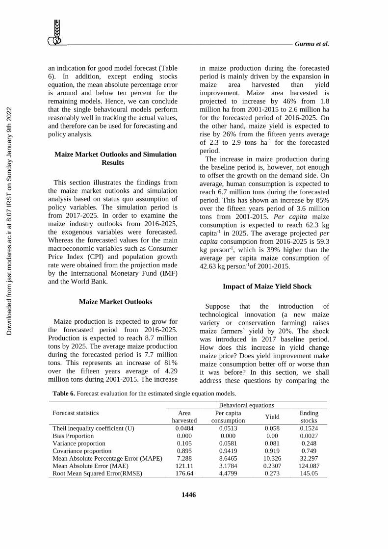
Table 6. Forecast evaluation for the estimated single equation models.

Forecast statistics

Behavioral equations

Area

harvested

Per capita

consumption Yield

Ending

stocks

Theil inequality coefficient (U) 0.0484 0.0513 0.058 0.1524

Bias Proportion 0.000 0.000 0.00 0.0027

Variance proportion 0.105 0.0581 0.081 0.248

Covariance proportion 0.895 0.9419 0.919 0.749

Mean Absolute Percentage Error (MAPE) 7.288 8.6465 10.326 32.297

Mean Absolute Error (MAE) 121.11 3.1784 0.2307 124.087

Root Mean Squared Error(RMSE) 176.64 4.4799 0.273 145.05

an indication for good model forecast (Table

6). In addition, except ending stocks

equation, the mean absolute percentage error

is around and below ten percent for the

remaining models. Hence, we can conclude

that the single behavioural models perform

reasonably well in tracking the actual values,

and therefore can be used for forecasting and

policy analysis.

Maize Market Outlooks and Simulation

Results

This section illustrates the findings from

the maize market outlooks and simulation

analysis based on status quo assumption of

policy variables. The simulation period is

from 2017-2025. In order to examine the

maize industry outlooks from 2016-2025,

the exogenous variables were forecasted.

Whereas the forecasted values for the main

macroeconomic variables such as Consumer

Price Index (CPI) and population growth

rate were obtained from the projection made

by the International Monetary Fund (IMF)

and the World Bank.

Maize Market Outlooks

Maize production is expected to grow for

the forecasted period from 2016-2025.

Production is expected to reach 8.7 million

tons by 2025. The average maize production

during the forecasted period is 7.7 million

tons. This represents an increase of 81%

over the fifteen years average of 4.29

million tons during 2001-2015. The increase

in maize production during the forecasted

period is mainly driven by the expansion in

maize area harvested than yield

improvement. Maize area harvested is

projected to increase by 46% from 1.8

million ha from 2001-2015 to 2.6 million ha

for the forecasted period of 2016-2025. On

the other hand, maize yield is expected to

rise by 26% from the fifteen years average

of 2.3 to 2.9 tons ha-1 for the forecasted

period.

The increase in maize production during

the baseline period is, however, not enough

to offset the growth on the demand side. On

average, human consumption is expected to

reach 6.7 million tons during the forecasted

period. This has shown an increase by 85%

over the fifteen years period of 3.6 million

tons from 2001-2015. Per capita maize

consumption is expected to reach 62.3 kg

capita-1 in 2025. The average projected per

capita consumption from 2016-2025 is 59.3

kg person-1, which is 39% higher than the

average per capita maize consumption of

42.63 kg person-1of 2001-2015.

Impact of Maize Yield Shock

Suppose that the introduction of

technological innovation (a new maize

variety or conservation farming) raises

maize farmers’ yield by 20%. The shock

was introduced in 2017 baseline period.

How does this increase in yield change

maize price? Does yield improvement make

maize consumption better off or worse than

it was before? In this section, we shall

address these questions by comparing the

Dow

nloa

ded

from

jast

.mod

ares

.ac.

ir at

8:0

7 IR

ST

on

Sun

day

Janu

ary

9th

2022

Maize Price Formation and Dynamics __________________________________________

1447

Table 7. Yield simulation and percentage increase compared to the baseline.

Affected components 2017 2018 2019 2020 2021 2022 2023 2024 2025

Maize yield tons ha-1

Baseline 2.86 2.91 2.89 2.88 2.92 2.93 2.96 2.94 3.00

Scenario 3.43 2.91 2.89 2.88 2.92 2.93 2.96 2.94 3.00

Absolute change 0.57 0.0 0.0 0.0 0.0 0.0 0.0 0.0 0.0

% Change 20% 0% 0% 0% 0% 0% 0% 0% 0%

Maize production Thousand tons

Baseline 6890 7193 7324 7498 7759 7972 8242 8374 8755

Scenario 8262 7193 7324 7498 7759 7972 8242 8374 8755

Absolute change 1373 0.0 0.0 0.0 0.0 0.0 0.0 0.0 0.0

% Change 20% 0% 0% 0% 0% 0% 0% 0% 0%

Domestic maize use Thousand tons

Baseline 6858 7126 7277 7455 7692 7909 8165 8325 8661

Scenario 7849 7337 7372 7498 7711 7918 8169 8326 8662

Absolute change 991 211 95 43 19 9 4 1 0

% Change 14% 3% 1% 1% 0% 0% 0% 0% 0%

Ending stocks Thousand tons

Baseline 441 509 556 599 666 728 805 854 948

Scenario 823 680 632 632 681 734 808 855 949

Absolute change 382 171 76 34 15 6 3 1 1

% Change 87% 34% 14% 6% 2% 1% 0% 0% 0%

Nominal wholesale

maize price ETB ton-1

Baseline 5733 5599 5845 5989 5717 5465 4855 4742 3759

Scenario 1061 4545 5347 5756 5609 5416 4833 4732 3755

Absolute change -4672 -1054 -498 -233 -108 -49 -22 -10 -4

% Change -81% -19% -9% -4% -2% -1% 0% 0% 0%

Source: Model outcomes.

simulation results with the baseline values.

We answer the question about the impact of

maize yield simulation in three steps.

Primarily, we examine the short-run and

long-run response of the different

components of the maize market model.

Then, we consider the direction and

proportion of the shift. In the end, we

quantify how these dynamic changes in the

supply and demand components translate

into the maize market equilibrium price.

The dynamic responses of the maize sub-

sector for a bumper harvest are summarised

in Table 7. From the yield simulation

analysis, it is clear that a 20% increase in

maize yield would result in an increase in

maize production by 20%. The impact of

yield simulation is more pronounced and

persistent on maize ending stocks and

nominal maize price. As compared to the

baseline, a 20% increase in maize yield

could reduce nominal maize price

substantially by 81%. In the short-run

(within the year), a positive change in yield

would increase maize ending stocks by 87%,

and the effect will also continue in the long-

run. A 20% positive change in maize yield

would lead to an increase in ending stocks

by 34, 14, 6, and 2% in 2018, 2019, 2020,

and 2021, respectively. A moderate impact

is noticed on domestic maize use; a 20%

change in maize yield could increase

domestic maize use by 14%. Harvested

maize area has remained unaffected by a

Dow

nloa

ded

from

jast

.mod

ares

.ac.

ir at

8:0

7 IR

ST

on

Sun

day

Janu

ary

9th

2022

_______________________________________________________________________ Gurmu et al.

1448

Table 8. Descriptive results of the nominal wholesale maize market prices, July 2004 to March 2016

(ETB a 100 kg-1).

Markets Mean Std. Dev. Max Min Driving distance from Addis

Ababa (km)

Market

type

Addis Ababa 347.46 157.28 631 123 - Surplus

Ambo 330.38 154.85 696 110 119 Surplus

Bahir Dar 343.93 169.82 770 112 552 Surplus

Debre-Birhan 356.44 164.87 663 123 132 Surplus

DM b 361.74 180.87 774 116 306 Surplus

Gondar 370.40 171.10 791 141 732 Surplus

Hosaena 376.68 182.01 801 127 228 Surplus

Jimma 316.61 157.59 718 100 352 Surplus

Nazareth 348.92 163.31 680 120 86.5 Surplus

Nekemete 312.28 155.94 635 96 318 Surplus

Shashemene 358.01 180.97 770 107 251 Surplus

Woliso 344.57 162.63 718 107 111 Surplus

Ziway 345.43 167.69 718 106 163 Surplus

Dese 358.07 160.01 690 129 388 Deficit

Mek’ele 385.17 179.46 904 99 762 Deficit

a Using the exchange rate of 13 May 2016, 1 Ethiopian Birr (ETB) was trading at around 0.046 USD. b Denotes Debre-Markos.

20% positive change in maize yield.

Long-run Relationships

This section examines the spatial maize

market integration among fifteen wholesale

maize markets in Ethiopia. Wholesale maize

markets are selected based on their

representativeness of crop production,

consumption areas, importance to the

national grain trade flow and data

availability. The descriptive results for the

wholesale maize prices are presented in

Table 8.

Since all the price series are non-stationary

and integrated of the same order I(1), co-

integration analysis is therefore appropriate

to investigate the long-run relation among

maize market prices. Given the large number

of maize markets, co-integration tests are

conducted in a pairwise fashion. Following

the results of Toda and Yamamoto (1995)

causality test. Addis Ababa maize market is

treated as an exogenous maize market. Thus,

in the subsequent co-integration analysis,

regional wholesale maize markets are paired

with Addis Ababa maize market. The use of

Addis Ababa maize price as a central market

is appropriate to this study because with 15

maize markets, there are 105 [(n2-n)/2]

possible market pairs.

Co-integration among maize market pairs

is tested using Johansen’s method (Johansen

1991). The results for the co-integrated

maize market pairs are presented in Table 9.

Trace and Maximal Eigen value test

statistics provided no conflicting results. In

both cases, the null of zero co-integrating

vectors (r= 0) was rejected. The last column

in table 9 presents the lag length selected for

long-run analysis of market pairs. Optimum

lags were chosen using the information

criterion [Akaike Information Criterion

(AIC), Schwarz Bayesian Criterion (SBC),

and Likelihood Ratio (LR)].

Results from Johansen co-integration tests

show that no co-integration was found

between Addis Ababa with regional maize

markets of Debre-Markos, Hosaena,

Shashemene, and Nazareth market pairs.

Given the proximity of Nazareth and Addis

Ababa, the absence of co-integration

between the two wholesale maize markets

was not expected. One possible cause for the

absence of co-integration between Nazareth

and Addis Ababa maize market could be the

Dow

nloa

ded

from

jast

.mod

ares

.ac.

ir at

8:0

7 IR

ST

on

Sun

day

Janu

ary

9th

2022

Maize Price Formation and Dynamics __________________________________________

1449

Table 9. Johansen tests for co-integration between wholesale maize market prices .

Markets Trace Ho Trace statistic Max Ho Max-Eigen statistic Lags

Addis-Ambo 𝑟 = 0 29.08*** 𝑟= 0 29.00***

2 𝑟 ≤ 1 0.075 𝑟= 1 0.075

Addis-BDa 𝑟 = 0 23.81*** 𝑟= 0 20.09**

2 𝑟 ≤ 1 3.72 𝑟= 1 3.72

Addis-DBa 𝑟 = 0 19.74*** 𝑟= 0 19.64***

3 𝑟 ≤ 1 0.10 𝑟= 1 0.10

Addis-Dese 𝑟 = 0 25.29*** 𝑟= 0 25.20***

2 𝑟 ≤ 1 0.09 𝑟= 1 0.09

Addis-Gondar 𝑟 = 0 20.38*** 𝑟= 0 20.37***

2 𝑟 ≤ 1 0.008 𝑟= 1 0.009

Addis-Jimma 𝑟 = 0 18.53*** 𝑟= 0 18.47***

9 𝑟 ≤ 1 0.06 𝑟= 1 0.06

Addis-Mek’ele 𝑟 = 0 13.71** 𝑟= 0 13.71**

3 𝑟 ≤ 1 0.003 𝑟= 1 0.003

Addis-Nekemete 𝑟 = 0 22.44** 𝑟= 0 18.87**

8 𝑟 ≤ 1 3.57 𝑟= 1 3.57

Addis-Woliso 𝑟 = 0 35.06*** 𝑟= 0 34.91***

2 𝑟 ≤ 1 0.15 𝑟= 1 0.15

Addis-Ziway 𝑟 = 0 27.01*** 𝑟= 0 26.87***

2 𝑟 ≤ 1 0.15 𝑟= 1 0.15

a BD and DB stand for Bahir Dar and Debre-Birhan markets. ***, **: Significance levels at 1 and 5%.

presence of structural breaks, which may

lead to misleading inference on co-

integration results. It is widely accepted that

the presence of structural breaks distorts the

validity of conventional unit root and co-

integration tests (Phillips, 1986; Perron,

1989). Therefore, tracing out the presence of

breaks in our data series is crucial,

especially in the presence of commodity

price crisis of 2008 and 2011. Furthermore,

since 2008, the Ethiopian government

intervened in domestic grain market in

response to high domestic commodity

prices. Hence, ignoring structural break test

in volatile commodity market environment

and with the presence of government

interventions in agricultural market might

falsely lead to non-rejection of the null

hypothesis of no co-integration.

The Bai and Perron (1998) breakpoint test is

used to analyse the effects of structural

breaks on maize markets integration. The

Bai and Perron (1998) structural break test is

useful to test unknown breaks in the price

series. The test uses the full sample and

adopts a different dummy variable for each

break. We further tested the presence of co-

integration by accounting the identified

structural breaks using the Stock and

Watson’s (1993) Dynamic Ordinary Least

Square approach (DOLS). The Johansen

method, being a full information technique,

is exposed to the problem that parameter

estimates in one equation are affected by any

misspecification in other equations (Azzam

& Hawdon, 1999:7). In contrast, the Stock

and Watson method is a robust single

equation approach, which overcomes the

simultaneity bias by incorporating leads and

lags of first differences of the regressors,

and for serially correlated errors by a

Generalized Least Squares (GLS) procedure.

For the sake of brevity, the mathematical

specifications and results for the Bai and

Perron (1998) breakpoint and DOLS tests

are not presented here. Interested readers can

refer to Rafailidis and Katrakilidis (2014) to

get a detailed explanation in these two

approaches.

Indeed, the conclusion for co-integration

tests altered when breakpoints were

considered in the analysis. Analysing co-

Dow

nloa

ded

from

jast

.mod

ares

.ac.

ir at

8:0

7 IR

ST

on

Sun

day

Janu

ary

9th

2022

_______________________________________________________________________ Gurmu et al.

1450

integration by taking into account breaks

gives a different story for maize markets

considered as non- cointegrated in

Johansen’s approach (see annex Tables 2-3).

Regional maize markets (Shashemene,

Nazareth, Debre-Markos, and Hosaena)

found to have no co-integration with Addis

Ababa maize market which became co-

integrated when structural breaks were taken

into account.

CONCLUSIONS

This study is an attempt to examine price

formation and dynamics in the Ethiopian

maize market. Results from the Johansen

tests reveal that out of 14 maize market

pairs, long-run relationship is confirmed in

11 market pairs. Nevertheless, the

conclusion for co-integration tests altered

when breakpoints were considered in the

analysis. When structural breaks were

considered in the price series, all regional

maize market pairs became co-integrated

with the central Addis Ababa maize market.

Co-integration of all maize market pairs

considered in this study is a reflection of

better spatial maize market linkages in

Ethiopia after the introduction of a

Structural Adjustment Program (SAP).

Findings from price formation

demonstrate that technological progress on

maize commodity has increased maize yield

in Ethiopia. As a result, maize production

has improved considerably. As demonstrated

in the yield simulation result, a 20% increase

in maize yield would increase maize

production by 20% and could reduce maize

price substantially by 81%. This may create

disincentives for producers. Thus any

interventions in the input sector should go

hand in hand with market development.

Given the imposition of an export ban on

maize, the only available market for farmers

and traders is the domestic market. The

domestic maize market outlet is also

confronted with many challenges. The major

challenge is the low maize demand in urban

areas. In spite of maize being the cheapest

source of calorie, consumption of processed

maize is not common in Ethiopia. As a

result, millers have allotted much of their

processing capacity to wheat flour and

products than maize flour. As explained by

(RATES, 2003), maize represents only 4%

of the total milling capacity in Ethiopia. The

challenge for expansion of maize processing

industry is the low demand in urban areas,

where the purchasing power is relatively

better. In such a situation, involvement in

maize processing industry is not feasible for

investors. In addition, the use of maize grain

and residue for poultry and livestock

production has not been widely practiced in

Ethiopia. Despite having the largest

livestock population in Africa, the use of

maize residues for silage making at

smallholder and industrial level is very

limited in Ethiopia. Therefore, expansion of

the industrial use of maize is an advisable

policy option. Governments could take steps

in enticing private sectors and small-scale

enterprises to take part in the sector, by

providing credit and infrastructure services.

Furthermore, linking private processors with

potential processed food buyers such as the

Purchase for Progress Program (P4P) of the

World Food Program (WFP) and productive

safety net programmes is a step in the right

direction. Thus, the output from private

processors will be channelled to food

insecure or drought prone areas of Ethiopia

either for a relief or food for work

initiatives.

REFERENCES

1. Abate, T., Bekele, S., Abebe, M., Dagne,

W., Yilma, K., Kindie, T., Menale, K.,

Gezahegn, B., Berhanu, T. and Tolera, K.

2015. Factors that Transformed Maize

Productivity in Ethiopia. Food Sec., 7: 965–

981.

2. Alemu, Z. G., Oosthuizen, K. and van

Schalkwyk, H. D. 2003. Grain-Supply

Response in Ethiopia: An Error-Correction

Approach. Agrekon, 42: 389-404.

Dow

nloa

ded

from

jast

.mod

ares

.ac.

ir at

8:0

7 IR

ST

on

Sun

day

Janu

ary

9th

2022

Maize Price Formation and Dynamics __________________________________________

1451

3. Asche, F., Gjølberg, O. and Guttormsen, A.

G. 2012. Testing the Central Market

Hypothesis: A Multivariate Analysis of

Tanzania Sorghum Markets. Agri. Econ, 43:

115-123.

4. Azzam, A. A. and Hawdon, D.

1999. Estimating the Demand for Energy in

Jordan: A Stock-Watson Dynamic OLS

(DOLS) Approach. Surrey Energy

Economics Discussion Paper, University of

Surrey, UK.

5. Bai, J. and Perron, P. 1998. Estimating and

Testing Linear Models with Multiple

Structural Changes. Econometrica, 66: 47-

68.

6. Brooks, C. 2008. Introductory Econometrics

for Finance. Second Edition, Cambridge

University Press, UK.

7. Central Statistical Agency (CSA). 2011.

Agricultural Sample Survey 2010/2011. I.

Report on Area and Production of Major

Crops (Private Peasant Holdings, Meher

Season. Statistical bulletin, Addis Ababa.

8. Chapoto, A. and Jayne, T. 2009. The

Impacts of Trade Barriers and Market

Interventions on Maize Price Predictability:

Evidence from Eastern and Southern Africa.

International Development Draft Working

Paper 102, Michigan State University.

9. De, Z. H. O. U. and Koemle, D. 2015. Price

Transmission in Hog and Feed Markets of

China. J. Int. Agri., 14(6): 1122-1129.

10. Diao, X., Kennedy, A., Mabiso, A. and

Pradesha, A. 2013. Economy Wide Impact

of Maize Export Bans on Agricultural

Growth and Household Welfare in Tanzania:

A Dynamic Computable General

Equilibrium Model Analysis. International

Food Policy Research Institute (IFPRI),

Discussion Paper 01287, Washington, DC.

11. Dickey, D. A., and Fuller, W. A. 1979.

Distribution of the Estimator for

Autoregressive Time Series with a Unit

Root. J. A. Stat. Ass, 74(366): 427-431.

12. Getnet, K., Verbeke, W. and Viaene, J.

2005. Modelling Spatial Price Transmission

in the Grain Markets of Ethiopia with an

Application of ARDL Approach to White

Teff. Agri. Econ., 33: 491-502.

13. Jaleta, M. and Gebermedhin, B. 2009. Price

Co-Integration Analyses of Food Crop

Markets: The Case of Wheat and Teff

Commodities in Northern Ethiopia. The

International Association of Agricultural

Economists Conference, Beijing, China;

August 16-22, 2009.

14. Johansen, S. and Juselius, K. 1990.

Maximum Likelihood Estimation and

Inference on Co-integration with

Applications to the Demand for Money. Ox.

B. Econ. Stat., 52: 169-210.

15. Johansen, S. 1991. Estimation and

Hypothesis Testing of Co-Integration

Vectors in Gaussian Vector Autoregressive

Models. Econometrica, 59(6): 1551-1580.

16. Kelbore, Z. G. 2013. Transmission of World

Food Prices to Domestic Market: The

Ethiopian Case. University of Trento.

Retrieved from [https://mpra.ub.uni-

muenchen.de/49712].

17. Negassa, A., Myers, R. and Gabre-Madhin,

E. 2004. Grain Marketing Policy Changes

and Spatial Efficiency of Maize and Wheat

Markets in Ethiopia. MTDI Discussion

Paper 66, International Food Policy

Research Institute (IFPRI), Washington, DC

18. Perron, P. 1989. The Great Crash, the Oil

Price Shock, and the Unit Root Hypothesis.

Econometrica, 57: 1361-1401.

19. Phillips, P. C. B. 1986. Understanding

Spurious Regression in Econometrics, J.

Econom., 33: 311-340.

20. Pindyck, R. S. and Rubinfeld, D. L. 1991.

Econometric Models and Economic

Forecasts. McGraw-Hill, NewYork.

21. Porteous, O. C. 2012. Empirical Effects of

Short-Term Export Bans: The Case of

African Maize. Working Paper, Department

of Agricultural Economics, University of

California, Berkeley.

22. Rafailidis, P. and Katrakilidis, C. 2014. The

Relationship between Oil Prices and Stock

Prices: A Non-Linear Asymmetric Co-

Integration Approach, Ap. Fin. Econ., 24:

793-800.

23. Ravallion, M. 1986. Testing Market

Integration. A. J. Agr. Econ., 68(1): 102-09.

24. Regional Agricultural Trade Expansion

Support Programme (RATES). 2003. Maize

market Assessment and Baseline Study for

Ethiopia, Nairobi, Kenya.

25. Stock, J. H. and Watson, M. W. 1993. A

Simple Estimate of Co-Integrating Vector in

Higher Ordered Integrated Systems,

Econometrica, 61(4): 783-820.

26. Tamru, S. 2013. Spatial Integration of

Cereal Markets in Ethiopia. Ethiopia

Strategy Support Program - Ethiopian

Dow

nloa

ded

from

jast

.mod

ares

.ac.

ir at

8:0

7 IR

ST

on

Sun

day

Janu

ary

9th

2022

_______________________________________________________________________ Gurmu et al.

1452

Development Research Institute, Addis

Ababa, Ethiopia.

27. The Food and Agriculture Organization

(FAO). 2015. FAOSTAT Production

Database. Retrieved 05/11/2015,

http:/faostat3.fao.org/download.

28. Toda, H. Y. and Yamamoto, T. 1995.

Statistical Inference in Vector Auto-

Regressions with Partially Integrated

Processes. J. Econ. 66:225–250.

29. Tripathi, A. 2008. Estimation of Agricultural

Supply Response Using Co-Integration

Approach. Indira Gandhi Institute of

Development Research, Mumbai.

30. Ulimwengu, J. M., Workneh, S. and Paulos,

Z. 2009. Impact of Soaring Food Price in

Ethiopia: Does Location Matter? IFPRI.

31. United States Department of Agriculture

(USDA). 2015. Commodity Database.

Available:

http://apps.fas.usda.gov/psdonline/psdquery.

aspx [2015, 24 November].

اتیوپی ذرت بازار در قیمت پویایی و گیری شکل سازی مدل

و ر. حسنم. ی. گورمو، ف. میر،

چکیده

یک جزئی تعادل .است اتیوپی ذرت بازار در قیمت پویایی و گیری شکل بررسی مطالعه اینهدف

( برایthe Johansen’s co-integration approaches) یوهانسن سازی همگام روشهای و کالا

یافته .گرفت قرار استفاده مورد اتیوپی ذرت فروش در بازار ادغام و ذرت قیمت بررسی شکل گیری

شده، افزایش یابد. بینی پیش دوره طی ذرت رود تولیدانتظار می نشان میدهد که ذرت صنعت های

تحلیل و تجزیه اگرچه افزایش تولید ذرت، برای جبران نیاز و تقاضای در حال رشد کافی نبوده است. از

18 تواند منجر به کاهش می ذرت افزایش در عملکرد ٪02 که مشخص شد عملکرد، سازی شبیه

ذرت فروشی عمده بازارهای که داد نشان انباشتگی هم تحلیل و تجزیه .شود ذرت اسمی درصدی قیمت

با مرتبط اطلاعات بهتر و بیشتر انتقال گر داشته اند که نشان بیشتری کارایی اخیر های سال در اتیوپی

. باشد می ذرت محصولات عمده تولید و مصرف بازار در قیمت

Dow

nloa

ded

from

jast

.mod

ares

.ac.

ir at

8:0

7 IR

ST

on

Sun

day

Janu

ary

9th

2022