Embed Size (px)
Citation preview
Chapter 7Calculation of Gibbs Energy of Solvation
7.1 Theory – Link Between Microscopic and MacroscopicWorld
In the next chapters, a short summary with regard to link the microscopic and macro-scopic world is given. For a more detailed description, the reader is referred to theliterature (van Gunsteren and Berendsen 1987; Jensen 1999; Frenkel and Smit 2002;van der Spoel et al. 2005).
7.1.1 Statistical Mechanical Basics
In this chapter we deal with the problem to connect a model or a microscopic pictureof matter to measurable macroscopic quantities. Linking these two worlds representsthe only possibility to validate models and gain insight into the molecular processes.Referring to the chapter of thermodynamical basics we established a model for theligand receptor interaction by formulating the equilibrium
L + R � LR (7.1)
characterized by its equilibrium constant, a measurable quantity:
K = cLRco
cLcR
(7.2)
To understand the processes leading to this equilibrium constant on a molecular level,we remember the fundamental equation resulting from the first and second law ofthermodynamics in the case of constant pressure and temperature:
�Go = −RT ln K. (7.3)
Because we transfer the measurable quantity K into the energetic quantity �Go wemake the first move to answer our central question. Obviously the next step is the
A. Strasser, H.-J. Wittmann, Modelling of GPCRs, 75DOI 10.1007/978-94-007-4596-4_7, © Springer Science+Business Media Dordrecht 2013
76 7 Calculation of Gibbs Energy of Solvation
connection of �Go to the interactions which take place when the ligand L leaves itssolvation state and enters the receptor R to form the complex LR. This link is givenby the concepts of Classical Statistical Mechanics in combination with QuantumMechanics. As formerly stated (Chap. 1), Quantum Mechanics would be the bestchoice for describing the behaviour of matter in a microscopic world but up to now itis impossible to handle large biochemical systems. So we use the Classical StatisticalMechanics which uses the Hamiltonian function
H ( �p, �r) = Ekin( �p) + Epot(�r) (7.4)
the sum of the total kinetic (Ekin) and the potential energy (Epot) as a central function tocalculate macroscopic quantities. H depends on the momenta ( �p) and the coordinates(�r) of all species present in the system of interest. Because we are interested in theequilibrium state of a system, H depends not explicitly on time. The expression forthe kinetic part of H is the sum over the kinetic energies of all species i:
Ekin( �p) =∑
i
�p2i
2mi
(7.5)
where mi denotes the mass and �pi the momentum of a particle i. The potential energyEpot(�r) comprises energies resulting from binding interactions, ion-ion, ion-dipoleor dipole-dipole interactions. Note, that the Hamiltonian function does not containvariables like the pressure p or the temperature T. These parameters appear in theexpressions of macroscopic quantities like the internal energy U of a system withfixed volume, temperature and number of particles, which will read as:
U (V , T , N ) = σV
QV
∫. . .
∫H ( �pi , �ri) exp
(−H ( �pi , �ri)
kT
)d �pid�ri (7.6)
where
QV = σV
∫. . .
∫exp
(−H ( �pi , �ri)
kT
)d �pid�ri (7.7)
k and T denote the Boltzmann constant and the temperature, N is the total number ofparticles in the system and σV is a normalisation constant. The integration is extendedover all values of the momenta and coordinates of all species i present in the system.The quantity QV is called the partition function at constant volume. Having a closerlook onto the Eqs. 7.6 and 7.7 U is identified as the mean value of the Hamiltonianfunction H over the so called phase space given by all the momenta and coordinates.Referring to a system with fixed pressure, temperature and number of particles we get:
H (p, T , N ) = σp
Qp
∫ ∫. . .
∫(H ( �pi , �ri) + pV )
· exp
(−H ( �pi , �ri) + pV
kT
)d �pid�ridV (7.8)
7.1 Theory – Link Between Microscopic and Macroscopic World 77
where
Qp = σp
∫ ∫. . .
∫exp
(−H ( �pi , �ri) + pV
kT
)d �pid�ridV (7.9)
is the partition function at constant pressure with the normalisation constant σp.Equations 7.8 and 7.9 contain the product of the pressure p and the volume V totransform the internal energy U into the enthalpy H, which must not be mixed upwith the Hamiltonian function H ( �p, �r). The Gibbs energy for a system at constantpressure, temperature and number of particles reads:
G = −kT ln Qp. (7.10)
It should be taken into consideration that the Gibbs energy G does not represent amean value, like the internal energy U or the enthalpy H, which will lead to newconcepts in the calculation of this quantity in the framework of Molecular Dynamics.
So, making use of the concepts of Statistical Mechanics we are able to calculateall important thermodynamical quantities after formulating the potential energy Epot.We therefore should be able to calculate measurable quantities like the ligand receptorassociation constant and compare the results with experimental values in order torefine our models.
7.1.2 From Potential Energy to the Chemical Potential
To calculate the equilibrium constant for the association process, Eq. 7.1, weremember the equation from the chapter of thermodynamical basics:
�Go = μoLR − μo
L − μoR. (7.11)
Because the chemical potential of each species LR, L or R means its Gibbs energy permole in accordance to Eq. 7.10 we have to evaluate the partition function Qp for con-stant pressure and constant temperature of an appropriate system, containing a num-ber of particles LR, L or R, which equals the Avogadro number NA, considering theparticular reference state. After defining the potential energy Epot(�r) we have to inte-grate over the whole phase space, which indeed is a very difficult task as this functionwill not be given in a simple analytical form. There are attempts to solve this problemwith the so-called Monte Carlo method (Metropolis 1987; Bouzida et al. 1992), butthis procedure takes a lot of time and the results very often are not satisfactory. Forlarge biochemical systems, the Molecular Dynamics is a widely accepted alternative(Christen and van Gunsteren 2008). This concept uses the Newton equation of mo-tion to follow the evolution of an arbitrary system with time, i. e. we will monitor allproperties of interest, for example the potential and kinetic energy of our system, intheir dependence of time. But now another problem arises in defining the equilibriumstate and calculating the corresponding macroscopic quantities U, H and G.
78 7 Calculation of Gibbs Energy of Solvation
First we postulate the equality between the mean values in phase space and themean on time scale from MD calculations, which is applicable for the quantities Uand H. Having a look on Eq. 7.10 we see that this concept does not hold for theGibbs energy. So there is no simple possibility to calculate this important quantityand therefore no way to estimate the equilibrium constant on the base of MolecularDynamics. To overcome this problem, the concept of perturbation with respect tothe potential energy is introduced. Suppose we have a system at constant pressure,temperature and constant number of particles. We indicate this state as state “1” andaccording to Eq. 7.9 the partition function Qp(1) for an arbitrary species is given bythe equation:
Qp(1) =∫ ∫
. . .
∫exp
(−H (1) ( �pi , �ri) + pV
kT
)d �pid�ridV . (7.12)
Now assume the Hamiltonian energy of our system has changed to state “2” byvariation of the particle interactions for example. We will then write the partitionfunction Qp(2):
Qp(2) =∫ ∫
. . .
∫exp
(−H (2) ( �pi , �ri) + pV
kT
)d �pid�ridV . (7.13)
Calculating the Gibbs energy for example of state “2” according to Eq. 7.10 yields:
G(2) = −kT ln Qp(2). (7.14)
Let us reformulate this equation in the following way:
G(2) = −kT ln
(Qp(1)Qp(2)
Qp(1)
). (7.15)
To what extent does this mathematical manipulation help us to solve our problem?First we can write the right hand side of Eq. 7.15 in the following form:
G(2) = −kT ln (Qp(1)) − kT lnQp(2)
Qp(1)(7.16)
and making use of Eq. 7.10, we have
G(2) = G(1) − kT lnQp(2)
Qp(1). (7.17)
Next we will reformulate Qp(2):
Qp(2) = ∫ ∫. . .
∫exp
(−H (2) ( �pi , �ri) + pV − (H (1) ( �pi , �ri) + pV )
kT
)
· exp
(−H (1) ( �pi , �ri) + pV
kT
)d �pid�ridV
(7.18)
7.1 Theory – Link Between Microscopic and Macroscopic World 79
which only means to multiply the integrand of Eq. 7.13 by one. Now, the resultantterm Qp(2)�Qp(1) represents the phase mean of the quantity
exp
(−H (2) ( �pi , �ri) + pV − (H (1) ( �pi , �ri) + pV )
kT
). (7.19)
This result is very important for the Molecular Dynamics simulation procedure be-cause this phase mean corresponds to the mean in time scale. We follow the timeevolution of our system in state “1” and calculate H(2) for the same set of variables�pi and �ri . The result represents the difference G(2)−G(1) due to a change in thepotential energy between the states 1 and 2. So we are able to use the MD simulationmethod to calculate a difference of the Gibbs energy for two distinct states of oursystem with the help of the so-called thermodynamic perturbation formula.
7.1.3 The Concept of the Coupling Parameter Within MDSimulations
The mentioned procedure for calculating the mean according to Eq. 7.18 sometimesleads to convergence problems in MD simulations especially if state “2” energeti-cally is far from state “1”. As a workaround to get the term G(2)−G(1) a stepwiseintegration based on small differences of the Hamiltonian energies between neigh-bouring states could be performed. Returning to Eq. 7.10 we introduce a so-calledcoupling parameter λ which described the state of the system. Therefore, a variationof λ indicates a change of the system state and we can write
G(λ) = −kT ln (Qp(λ)) (7.20)
where Qp(λ) reads
Qp(λ) =∫ ∫
. . .
∫exp
(−H (λ) ( �pi , �ri) + p · V
k · T
)d �pid�ridV . (7.21)
Within the framework of the coupling-parameter concept, the Coulomb potential forinstance between two sites i and j separated by the distance rij for example, is definedby the following equation:
Eel = 1
4πεorij
((1 − λ)q (1)
i q(1)j + λq
(2)i q
(2)j
). (7.22)
Therein, the superscripts (1) and (2) refer to the state 1 and 2, respectively.
80 7 Calculation of Gibbs Energy of Solvation
A differential small change in λ, dλ will lead to the following expression for Qp:
dQp(λ)
dλ= − 1
kT
∫ ∫. . .
∫dH (λ) ( �pi , �ri)
dλ
· exp
(−H (λ) ( �pi , �ri) + pV
kT
)d �pid�ridV (7.23)
and according to Eq. 7.10
dG(λ)
dλ= − kT
Qp(λ)
dQp(λ)
dλ(7.24)
where the term dQ(λ)dλ
1Qp(λ) represents a mean value of dH (λ)( �pi ,�ri )�dλ and so we are
able to calculate dG(λ)�dλ as a function of λ by MD simulation. A numerical integra-tion procedure will yield the desired term G(2)−G(1). The concept of the couplingparameter λ could be thought as special case of the energy perturbation conceptmentioned in the foregoing section.
In the next two sections, we will apply the concept of the coupling parameter tothe calculation of the Gibbs energy of solvation for the system ethanol/water andsubsequently to the estimation of the equilibrium constant for the ligand bindingprocess.
7.2 Examples – Conceptual and Practical Considerations
7.2.1 Example 1: Ethanol in Water – Conceptual Considerations
From a thermodynamic point of view, the desired solvation energy requires thecalculation of the reference chemical potentials (at the pressure of 1 bar and thetemperature of 298.15 K), when transferring one mole of ethanol from the ideal gasstate into the solvent (water), forming an ideal solution of concentration 1 mol/l.
�Gosol = μo
EtOH − μo,gEtOH. (7.25)
Applying the coupling parameter concept, we will start from a system state 1, whichcorresponds to the solution of nEtOH moles of ethanol and nH2O moles of water. Inthe next step, we will switch off all interactions between ethanol and water, arrivingin a system state 2, comprising of the pure solvent and a “solute”, which will beconsidered as an ideal gas. The Gibbs energy corresponding to state 1 will read:
G(1) = nEtOH
(μo
EtOH + RT lncEtOH
co
)+ nH2O
(μ∗
H2O + RT ln xH2O
). (7.26)
7.2 Examples – Conceptual and Practical Considerations 81
Here, we assume a dilute solution of ethanol in water in order to neglect the interac-tions between the solute molecules and the influence of remaining ethanol moleculeson the interaction of a particular solute molecule with the solvent. This assumptionallows omitting the activity coefficients (compare Chap. 10) and so we are able toestablish an ideal solution. The reference chemical potential of the solvent μ∗
H2O
refers to the pure solvent at 1 bar and 298.15 K. The corresponding concentrationvariable is then given by the mole fraction xH2O.
For state 2, we may write:
G(2) = nEtOHμo,gEtOH + nH2Oμ∗
H2O (7.27)
where μo,gEtOH denotes the reference state of the ideal gas ethanol at standard pressure.
Taking the difference G(1)−G(2) we arrive at:
G(1) − G(2) = nEtOH(μo
EtOH − μo,gEtOH
) + nEtOHRT lncEtOH
co
+ nH2ORT ln xH2O (7.28)
because the terms containing the reference chemical potential for the solvent canceland the first term within parenthesis of the right hand side of Eq. 7.28 corresponds tothe Gibbs energy of solvation. The left hand side of Eq. 7.28 will be calculated withthe help of MD-coupling-parameter concept and so requires to set up an appropriatesystem. In the framework of GROMACS MD simulations, the quantity mole may bereplaced by particle numbers. Thus, one mole of some species means one particle ofthe species in the simulation. To set up the system, one would choose one moleculeof ethanol, firstly, to fulfil the requirement of neglecting the formerly discussedinteractions, and secondly, to have the desired term μo
EtOH − μo,gEtOH isolated on the
right hand side of Eq. 7.28. The next problem is the choice of the quantity nH2O. Ofcourse, one could try to use a number of water molecules in such a way, that the twoconcentration terms on the right hand side of Eq. 7.28 would cancel:
RT
(ln
cEtOH
co
+ nH2O lnnH2O
1 mol + nH2O
)= 0. (7.29)
The calculated difference G(1)−G(2) equals the Gibbs energy of solvation in thiscase. The concentration term cEtOH may be written approximately as
cEtOH = nEtOHρH2O
nEtOHMEtOH + nH2OMH2O
(7.30)
where the symbols MEtOH and MH2O denote the molar masses of the solute andthe solvent, ρH2O means the density of water and will be substituted in the case ofdilute solution by 1 kg/l. Taking into account nEtOH = 1 mol, we get an equation forestimating nH2O , which, after solving numerically, exhibits the result of 18 watermolecules. However, for a simulation with periodic boundary conditions, the systemcomprised of 19 molecules will be too small. So, the question arises, how manywater molecules to use and how to treat the concentration terms in Eq. 7.28. To set
82 7 Calculation of Gibbs Energy of Solvation
up a system large enough for an exact simulation, the box size should be as large aspossible, i.e. nH2O is much larger than nEtOH, xH2O will be approximately one andthe term ln xH2O will reach zero. But if we choose nEtOH = 1 mol and calculate theterm nH2ORT ln xH2O for several numbers of water molecules, we would conjecturethe limiting value −RT. So, what is the correct result? As we demand a large numberof solvent particles, we already see that the logarithm of the mole fraction of thesolvent reaches the value zero, but this term is multiplied by the nH2O itself. Onthe one hand, we have a term approaching zero, but on the other hand we havea term getting larger and larger. To achieve the correct result of this product, wehave to use the so-called rule of L’Hospital which tells us that the limiting value ofthe expression will be −RT. If we choose NH2O = 512, we get xH2O = 0.998051and nH2ORT ln xH2O = −2.476 kJ per mol ethanol. For NH2O = 3,000, xH2O =0.999667 and nH2ORT ln xH2O = −2.477 kJ per mole ethanol, which is close to thelimiting value − RT (−2.479 kJ per mole ethanol) at a temperature of 298.15 K. So,a choice of the number of solvent molecules between 512 and 3,000 or higher willlead to a constant term of approximately −RT in Eq. 7.28. Now let us have a lookonto the concentration term in Eq. 7.28:
nEtOHRT lncEtOH
co
. (7.31)
Setting nEtOH equal to 1 mol, the value of cEtOH is determined by the choice of thenumber of water molecules, which define the system volume. Having NH2O = 800,we get a cubic box size of 2.87538 nm atT = 298.15 K and p = 1 bar. The concentrationof ethanol for a box volume V is then given by
cEtOH = 1 mol
NAV(7.32)
with a value of 0.0698 mol/l. The corresponding energy term for 1 mol of ethanol willbecome RT ln cEtOH
co= −6.599 kJ. The experimental value of �Go
sol is −20.98 kJ/mol. Thus, the concentration term just calculated, represents a fraction of approxi-mate 30 % and the corresponding solvent term of about 12 %. To reduce the amountof corrections necessary for calculating solvation energies, Villa et al has given aworkaround of this problem by taking the number of solvent molecules as 3,000,placed in a cubic box of length 4.5 nm, using a so-called twin-range cut-off distanceof 0.8 and 1.4 nm, respectively (Villa and Mark 2002).
The partial charges of the sites of the solutes are adjusted to reproduce the exper-imental values of the quantity �Go
sol neglecting the discussed concentration terms.So the calculated difference G(1)−G(2) directly corresponds to the Gibbs energyof solvation. Referring to our present example, a number of 3,000 water moleculesand 1 mol molecule of ethanol gives rise to a mol fraction of water xH2O = 0.999667,whereas the molar concentration of ethanol reads as cEtOH = 0.01822 mol/l. At a tem-perature of 298.15 K, the concentration terms of Eq. 7.28 will influence the above
mentioned difference of the Gibbs energies by RT(
ln cEtOH
co+ nH2O ln xH2O
)=
−12.41 kJ per mol ethanol, which is about 60 % of the experimental value

7.2 Examples – Conceptual and Practical Considerations 83
Table 7.1 Differences inpotential and kinetic energyof one ethanol surrounded by3,000 water molecules fordifferent cut-off’s
Run Cut-off [nm] Epot [kJ/mol] Ekin [kJ/mol]
1 0.5 −85,911 33,4632 1.4 −128,801 33,4593 2.0 −128,968 33,458
−20.98 kJ/mol (Cabani et al. 1981). Thus, the evaluation of the parameters of anyforce-field, which should describe properties of solutions in an exact manner, has toconsider these facts to avoid artificial effects. As G(1)−G(2) is the quantity resultingfrom a simulation, the term to be subject of adjustment is given by:
G(1) − G(2) − RT
(ni ln
ci
co
+ nH2O ln xH2O
)= ni
(μo
i − μo,gi
)(7.33)
for an arbitrary species i.Another problem arises from the so-called cut-off distance for calculating the
coulomb and van der Waals interactions between sites during a MD simulation. Shortcut-off distances will fasten the calculation, but lead to more inaccurate results. Usingboundary conditions and the PME method, this cut-off must not exceed the half ofthe cubic box length. To get insight into the consequences for different values of thecut-off distance, we will analyze the total kinetic and potential energy of a systemcontaining 1 molecule of ethanol and 3,000 molecules of water at 1 bar and 298.15 K.For this, we do three independent runs of a 1,000 ps MD simulation and calculate themean of these energies over a time interval from 500 ps to 1,000 ps with the help ofthe GROMACS command g_energy. The result may look like given in Table 7.1:
We see, that the results corresponding to the first cut-off value differ considerablyfrom that of run 2 and 3, which exhibit nearly the same results with respect to thecomputational error. A 1,000 ps MD simulation with 3,000 water molecules andone molecule of ethanol using a twin-range cut-off between 0.8 and 1.4 nm (Villaand Mark 2002) exhibits a kinetic energy of 33,975 kJ/mol and a potential energyof −130,183 kJ/mol. Both values are different to the values given in Table 7.1 andreflect the importance of the simulation conditions.
7.2.2 Example 2: Ligand-Receptor-Complexand Affinity – Conceptual Considerations
Now let us apply the concept, discussed so far to evaluate the equilibrium constantaccording to Eq. 7.3. To do so, we must have knowledge about the reference chemicalpotentials according to Eq. 7.11. To elucidate the application of coupling parameterslet us have a look on the system state 1 consisting of nL moles of ligand moleculesand nS moles of solvent molecules at a given pressure and temperature. We assumethat nS is much larger than nL. Thus, the interactions between the ligand particlesmay be neglected just as the influence of the ligand molecules on the solvation of
84 7 Calculation of Gibbs Energy of Solvation
a particular ligand molecule. The system state 2 will be defined for all interactionsbetween ligand and solvent particles switched off, so we have a system containingthe ligand as an ideal gas and the pure solvent. Making use of the concept of theforegoing section we are able to calculate the difference G(2)−G(1). We may writethe expressions for G(1) and G(2) from a thermodynamic point of view:
G(1) = nL ·(
μoL + RT ln
(cL
co
)+ nS · (
μ∗s + RT ln (xs)
)). (7.34)
Here, again for the solvent, we make use of the reference chemical potential for thepure state of water at 1 bar and 298.15 K.
G(2) = nLμo,gL + nsμ
∗s (7.35)
where μ∗s denote the reference chemical potential of the pure solvent with mole
fraction xS and μo,gL denotes the reference chemical potential of the ligand as an ideal
gas.Substracting G(1) from G(2) yields:
G(2) − G(1) = nL
(μ
o,gL − μo
L − RT ln
(cL
co
))
+ ns
(μ∗
s − μ∗s − RT ln (xs)
). (7.36)
As the terms for the reference potential of the solvent cancel the Eq. (7.36) nowreads:
G(2) − G(1) = nL
(μ
o,gL − μo
L − RT ln
(cL
co
))− nSRT ln (xS). (7.37)
Next we will do a similar calculation for the ligand-receptor-complex where theinteractions between the ligand and the receptor will be switched off. We define thestarting state 3 composed of nLR moles of ligand-receptor-complexes and nS molesof solvent where nS is much larger than nLR and nL. By switching of the interactionsbetween the ligand and the receptor, we arrive at state 4 comprising of the ligand asan ideal gas and the empty receptor located in the solvent. The Gibbs energy of state3, G(3), and state 4, G(4), are represented by the Eqs. 7.38 and 7.39:
G(3) = nLR
(μo
LR + RT ln
(cLR
co
))+ ns
(μ∗
s + RT ln (xs))
(7.38)
G(4) = nLμo,gL + nR
(μo
R + RT ln
(cR
co
))+ ns
(μ∗
s + RT ln (xs)). (7.39)
Formulating the difference G(4)−G(3), the entire solvent terms cancel and we get:
G(4) − G(3) = nLμo,gL + nR
(μo
R + RT ln
(cR
co
))
−nLR
(μo
LR + RT ln
(cLR
co
)).
(7.40)
7.2 Examples – Conceptual and Practical Considerations 85
Because the ligand, the receptor and the ligand-receptor-complex are charged gen-erally, appropriate counter ions have to be present in an electrically neutral solution.For the discussion of the thermodynamics of the association process, we presuppose,that these counter ions do not influence the formation of the ligand-receptor-complex.
For the process under consideration we have
nLR = nL = nR. (7.41)
So, the concentration terms cancel and the difference yields:
G(4) − G(3) = nL
(μ
o,gL + μo
R − μoLR
). (7.42)
Establishing the difference:
(G(2) − G(1)) − (G(4) − G(3)) (7.43)
will yield the following equation:
(G(2) − G(1)) − (G(4) − G(3)) = nL
(μo
LR − μoR − μo
L
)
− nLRT lncL
co
− nSRT ln xS (7.44)
because the terms containing μo,gL cancel. The first expression within parenthesis
on the right hand side of Eq. 7.44 equals the desired quantity �G◦ in the case ofnL = 1 mol. The second and third term represent the corrections analogous to thesolvation problem, discussed in this chapter. Applying the concept of the couplingparameter within the framework of MD simulations, we are able to evaluate theequilibrium constant for the association process, Eq. 7.1, according to Eq. 7.24.
7.2.3 Example 1: Ethanol in Water – Practical Considerations
After discussing the theoretical concept in the field of thermodynamics in combina-tion with thermodynamic integration method (coupling-parameter method), we willpresent the calculation of the Gibbs energy of solvation using the software packageGROMACS. Let us exemplary calculate the Gibbs energy of solvation for ethanolin water. Therefore, the following steps have to be performed.
� Construct the molecule, for which the Gibbs energy of solvation shouldbe calculated and save the coordinates as pdb-file
� Contact the PRODRG-Server in order to obtain the GROMACS-coordinates as a gro-file and the GROMACS-topology as a top-file (seeChap. 4)
� Change the size of the simulation box in an appropriate manner� Minimize your molecule in gas phase (see Chap. 6)
86 7 Calculation of Gibbs Energy of Solvation
� Calculate dG�dλ for gas phase via MD simulation, for example via the shellscript gibbs_energy (see below)
� Center your solute, obtained by item 4 in the simulation box� Solvate your solute with the desired solvens using the GROMACS
command genbox� Adopt your mdp-file for minimization, if necessary� Minimize your simulation box (solute in solvens)� Adopt your mdp-file for molecular dynamic simulation, if necessary� Calculate dG�dλ for ethanol in water via MD simulation, for example via
the shell script gibbs_energy (see below)
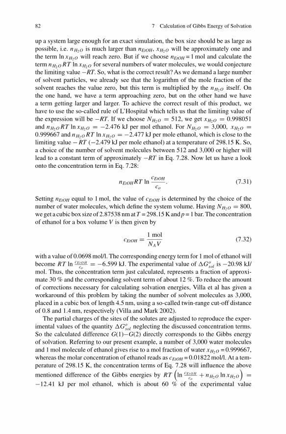
Fig. 7.1 Thermodynamiccycle for ethanol in water(coloured ligand: fullinteractions; grey ligand: noCoulomb and van der Waalsinteractions)
Each of the mentioned items will be explained now step by step: First, generatean appropriate gro- and top-file for ethanol, as described in detail in Chap. 4. Savethe files, shown explicitly in Chap. 4, as ethanol.gro and ethanol.itp. Inthe next step, one has to modify the topology file ethanol.itp. In the section[ atoms ], only the atom types, charges and masses for the state 1 are defined.To calculate the Gibbs energy of solvation according to the thermodynamic cycle(Fig. 7.1; Villa and Mark 2002), the solute has to be transferred into an ideal gas stateby switching of all the Coulomb and van der Waals interactions within ethanol.
The energy, which is necessary to remove all non-bonded internal interactions,like Coulomb- or van der Waals interaction for the solute in vacuum is representedby �Go
1 (Fig. 7.1). Therefore, all sites of state 1 are mutated gradually into dummysites, corresponding to state 2. In GROMACS, for example, a dummy is represented
7.2 Examples – Conceptual and Practical Considerations 87
by DUM, where all partial charges and van der Waals interaction parameters are setto zero. Therefore, in the section [ atoms ] three additional columns for type,charge and mass of the dummy sites are necessary. Setting the charges of all solutesites to zero and defining the site type DUM, switches off the Coulomb and van derWaals interactions between the sites of the solute. However, all internal, bondedinteractions and masses remain unchanged. The analogous energy term to removeall non-bonded internal interactions for the solute and between the solute and thesolvent is described by �Go
3 (Fig. 7.1), neglecting the concentration terms for ethanoland water as discussed in this chapter in the framework of parameter adjustment.Therefore, the same procedure as mentioned above for �Go
1 has to be performed.The energy, which is necessary to transfer the dummy solute from vacuum intosolvent is described by �Go
2 (Fig. 7.1). Since there is no interaction of the dummysolute with the remaining system, this value is zero. The values for �Go
1 and �Go3
can be calculated by appropriate MD simulations, as shown later. Subsequently, theGibbs energy of solvation of ethanol in water �Go
sol(EtOH) can be estimated via
�Gosol(EtOH) = �Go
1 − �Go3. (7.45)
In the following, the [ atoms ] section of ethanol.itp with the additionalcolumn is presented.
[ atoms ]; nr type resnr resid atom cgnr charge mass
1 CH3 1 DRG CAA 1 0.000 15.0350 DUM 0.0 15.03502 CH2 1 DRG CAC 1 0.266 14.0270 DUM 0.0 14.02703 OA 1 DRG OAB 1 −0.674 15.9994 DUM 0.0 15.99944 HO 1 DRG HAA 1 0.408 1.0080 DUM 0.0 1.0080
Save this file as ethanol.itp. Minimize the ethanol and save the resulting file asethanol_gas.gro. Solvate the minimized ethanol with an appropriate number of watermolecules, using the GROMACS commands editconf to center the solvent in thesimulation box and genbox for solvation. Minimize the box and save the file asethanol_sol.gro. Now, one can start the simulation to calculate the Gibbs en-ergy of solvation. Therefore, you would have to start a distinct number of subsequentmolecular dynamic simulations for discrete values of λ. Thereby, it should be takeninto account, to perform the calculations at least at eighteen values for λ, for example:0.0, 0.05, 0.1, 0.2, 0.3, 0.4, 0.45, 0.5, 0.55, 0.6, 0.7, 0.8, 0.9, 0.95, 0.975, 0.99, 0.995and 1.0. In general, a �λ of 0.1 can be used. But to avoid singularities around 0, 0.5and 1, at these regions, smaller �λ are recommended, as shown above. It is very use-ful to perform the calculations for aqueous and gaseous phase as in two different sub-directories aqueous and gaseous. Additionally, for each λ-calculation a separatesubdirectory in the subdirectory aqueous or gaseous should be used. Surely, youcan perform the simulations for each λ manually, but this is very inefficient. There-fore, it is more useful to use the shell script gibbs_energy, shown below. Usingthis script, all simulations of the aqueous or gaseous phase can be performed.
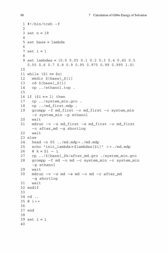
88 7 Calculation of Gibbs Energy of Solvation
1 #!/bin/tcsh −f23 set n = 1845 set base = lambda67 set i = 189 set lambdas = (0.0 0.05 0.1 0.2 0.3 0.4 0.45 0.5
0.55 0.6 0.7 0.8 0.9 0.95 0.975 0.99 0.995 1.0)1011 while ($i <= $n)12 mkdir ${base}_${i}13 cd ${base}_${i}14 cp ../ethanol.top .1516 if ($i = = 1) then17 cp ../system_min.gro .18 cp ../md_first.mdp .19 grompp −f md_first −o md_first −c system_min
−r system_min −p ethanol20 wait21 mdrun −v −s md_first −e md_first −o md_first
−c after_md −g shortlog22 wait23 else24 head -n 65 ../md.mdp>./md.mdp25 echo "init_lambda=$lambdas[$i]" >>./md.mdp26 @ k = $i − 127 cp ../${base}_$k/after_md.gro ./system_min.gro28 grompp −f md −o md −c system_min −r system_min
−p ethanol29 wait30 mdrun −v −s md −e md −o md −c after_md
−g shortlog31 wait32 endif3334 cd ..35 @ i++3637 end3839 set i = 140
7.2 Examples – Conceptual and Practical Considerations 89
41 while ( $i < = 18 )42 tail -n 100001 lambda_${i}/dgdl.xvg
> lambda_${i}/dgdl.dat43 echo "$i ‘average_gibbs lambda_${i}/dgdl.dat‘ "
>>lambda_gibbs.dat44 @ i++45 end
Before the script gibbs_energy can be started, the execute permission for theuser has to be set using the following command:
>chmod u+x gibbs_energy
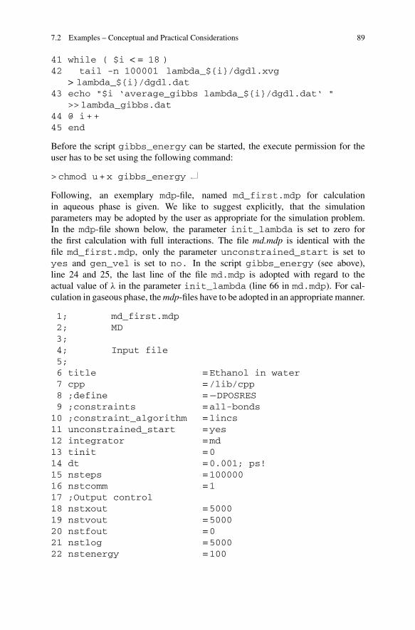
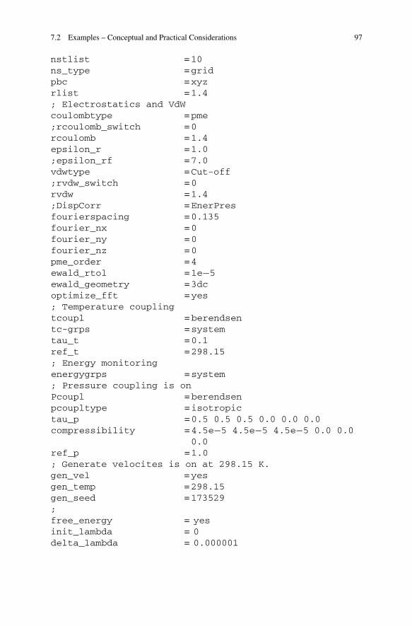
Following, an exemplary mdp-file, named md_first.mdp for calculationin aqueous phase is given. We like to suggest explicitly, that the simulationparameters may be adopted by the user as appropriate for the simulation problem.In the mdp-file shown below, the parameter init_lambda is set to zero forthe first calculation with full interactions. The file md.mdp is identical with thefile md_first.mdp, only the parameter unconstrained_start is set toyes and gen_vel is set to no. In the script gibbs_energy (see above),line 24 and 25, the last line of the file md.mdp is adopted with regard to theactual value of λ in the parameter init_lambda (line 66 in md.mdp). For cal-culation in gaseous phase, the mdp-files have to be adopted in an appropriate manner.
1; md_first.mdp2; MD3;4; Input file5;6 title =Ethanol in water7 cpp =/lib/cpp8 ;define = −DPOSRES9 ;constraints =all-bonds10 ;constraint_algorithm =lincs11 unconstrained_start =yes12 integrator =md13 tinit =014 dt =0.001; ps!15 nsteps =10000016 nstcomm =117 ;Output control18 nstxout =500019 nstvout =500020 nstfout =021 nstlog =500022 nstenergy =100

90 7 Calculation of Gibbs Energy of Solvation
23 ;Neighbor searching24 nstlist =1025 ns_type =grid26 pbc =xyz27 rlist =1.428 ;Electrostatics and VdW29 coulombtype =PME30 ;rcoulomb_switch =031 rcoulomb =1.432 epsilon_r =1.033 ;epsilon_rf =7.034 vdwtype =Cut-off35 ;rvdw_switch =036 rvdw =1.437 ;DispCorr =EnerPres38 fourierspacing =0.1239 fourier_nx =040 fourier_ny =041 fourier_nz =042 pme_order =443 ewald_rtol =1e-544 optimize_fft =yes45 ; Temperature coupling46 tcoupl =berendsen47 tc-grps =LIG SOL48 tau_t =0.1 0.149 ref_t =298 29850 ; Energy monitoring51 energygrps =LIG SOL52 ; Pressure coupling is not on53 Pcoupl =berendsen54 pcoupltype =isotropic55 tau_p =0.5 0.5 0.5 0.0 0.0 0.056 compressibility =4.5e-5 4.5e-5 4.5e-5 0.0
0.0 0.057 ref_p =1.058 ; Generate velocites is on at 298 K.59 gen_vel =yes60 gen_temp =29861 gen_seed =17352962 ; Free Energy Calculation63 free_energy =yes64 sc-alpha =1.565 sc-power =266 init_lambda =0.0
7.2 Examples – Conceptual and Practical Considerations 91
The files dgdl.dat, created by gibbs_energy contain two columns. The firstcolumn represents the time and the second one the values dG�dλ. To calculate the meanof dG�dλ at one λ, the gawk-script average_gibbs, presented below, can beused:
#!/usr/bin/gawk -f
BEGIN {s=0; n=0}
{n++; s=s+$2}
END {print s/n}
Before the script average_gibbs can be started, the execute permission for theuser has to be set using the following command:
>chmod u+x average_gibbs
Additionally, average_gibbs must reside in the same directory, as gibbs_energy, because average_gibbs is started in line 43 of gibbs_energy.Thus, after gibbs_energy has completed, a file named lambda_gibbs.datis created, containing λ in the first column and the mean of dG�dλ in the secondcolumn. With the help of the script integrate, shown later on, the integration canbe performed.
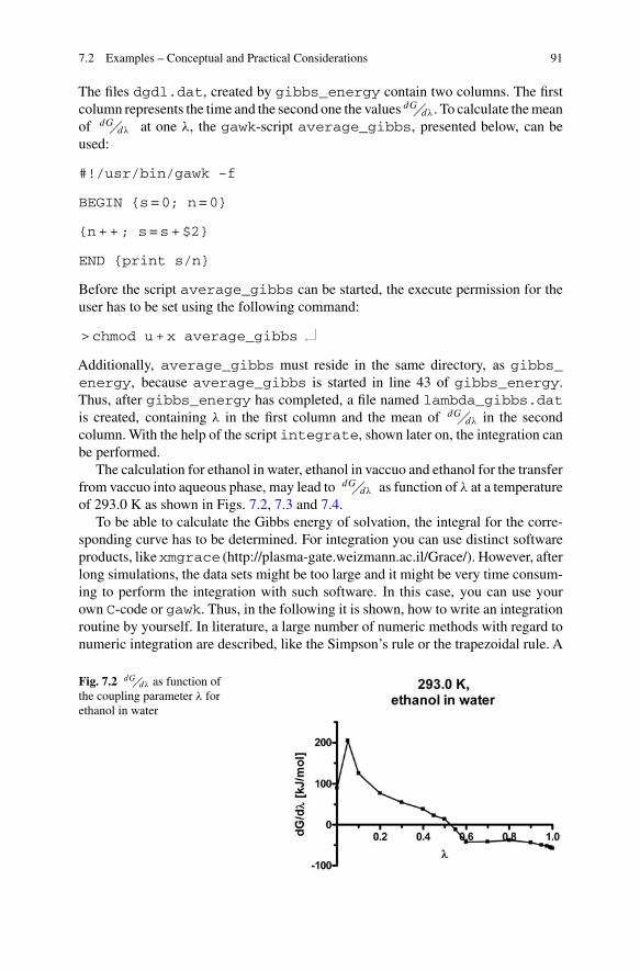
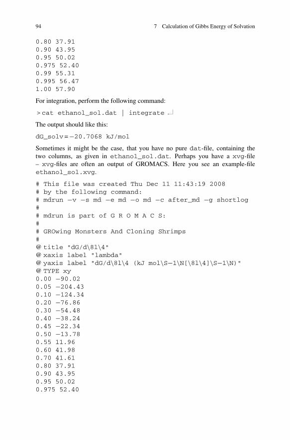
The calculation for ethanol in water, ethanol in vaccuo and ethanol for the transferfrom vaccuo into aqueous phase, may lead to dG�dλ as function of λ at a temperatureof 293.0 K as shown in Figs. 7.2, 7.3 and 7.4.
To be able to calculate the Gibbs energy of solvation, the integral for the corre-sponding curve has to be determined. For integration you can use distinct softwareproducts, likexmgrace (http://plasma-gate.weizmann.ac.il/Grace/). However, afterlong simulations, the data sets might be too large and it might be very time consum-ing to perform the integration with such software. In this case, you can use yourown C-code or gawk. Thus, in the following it is shown, how to write an integrationroutine by yourself. In literature, a large number of numeric methods with regard tonumeric integration are described, like the Simpson’s rule or the trapezoidal rule. A
Fig. 7.2 dG�dλ as function ofthe coupling parameter λ forethanol in water
92 7 Calculation of Gibbs Energy of Solvation
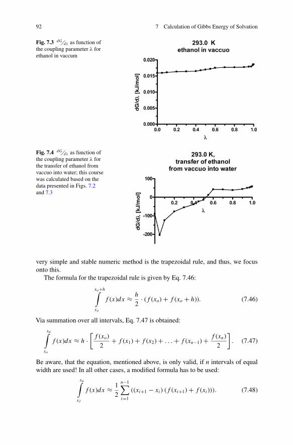
Fig. 7.3 dG�dλ as function ofthe coupling parameter λ forethanol in vaccum
Fig. 7.4 dG�dλ as function ofthe coupling parameter λ forthe transfer of ethanol fromvaccuo into water; this coursewas calculated based on thedata presented in Figs. 7.2and 7.3
very simple and stable numeric method is the trapezoidal rule, and thus, we focusonto this.
The formula for the trapezoidal rule is given by Eq. 7.46:
xo+h∫
xo
f (x)dx ≈ h
2· (f (xo) + f (xo + h)). (7.46)
Via summation over all intervals, Eq. 7.47 is obtained:
xn∫
xo
f (x)dx ≈ h ·[f (xo)
2+ f (x1) + f (x2) + . . . + f (xn−1) + f (xn)
2
]. (7.47)
Be aware, that the equation, mentioned above, is only valid, if n intervals of equalwidth are used! In all other cases, a modified formula has to be used:
xn∫
x1
f (x)dx ≈ 1
2
n−1∑
i=1
((xi+1 − xi) (f (xi+1) + f (xi))). (7.48)

7.2 Examples – Conceptual and Practical Considerations 93
Table 7.2 Derivative of the Gibbs energy with respect to the coupling parameter for the transfer ofethanol from vacuum into water at 293.0 K
λ 0.00 0.05 0.10 0.20 0.30 0.40dG/dλ [kJ/mol] −90.02 −204.43 −124.34 −76.86 −54.48 −38.24λ 0.45 0.50 0.55 0.60 0.70 0.80dG/dλ [kJ/mol] −22.34 −13.78 11.96 41.98 41.61 37.91λ 0.90 0.95 0.975 0.99 0.995 1.00dG/dλ [kJ/mol] 43.95 50.02 52.40 55.31 56.47 57.90
Therein, x0 corresponds to the lower bound of integration and xn to the upper boundof integration
Now, let us apply this integration method to the example ethanol in water, shownabove, in order to calculate the solvation energy. The data, presented in Fig. 7.4, aregiven in Table 7.2 and represent the derivative of the Gibbs energy with respect to λ
as a function of λ.The integration can easily be performed using Eq. 7.48 with the following
gawk-script, named integrate:
#!/usr/bin/gawk -f
BEGIN {s=0; n=0; OFS=’’’’}
{n++; x[n]=$1; y[n]=$2}
END {for(i=1;i<n;i++)s+=0.5*(x[i+1]−x[i])*(y[i+1]+y[i]);print ’’dG_solv=’’,s,’’ kJ/mol’’}
Now, you can open an editor, write the command sequences into the editor and savethe file with the name integrate. To test this script, you should first change yourfile access rights, using the following command:
>chmod u+x integrate
Next, create a file, containing the data shown in Table 7.2. In this example, we namethe file ethanol_sol.dat, which should look like this:
0.00 −90.020.05 −204.430.10 −124.340.20 −76.860.30 −54.480.40 −38.240.45 −22.340.50 −13.780.55 11.960.60 41.980.70 41.61
94 7 Calculation of Gibbs Energy of Solvation
0.80 37.910.90 43.950.95 50.020.975 52.400.99 55.310.995 56.471.00 57.90
For integration, perform the following command:
>cat ethanol_sol.dat | integrate
The output should like this:
dG_solv= −20.7068 kJ/mol
Sometimes it might be the case, that you have no pure dat-file, containing thetwo columns, as given in ethanol_sol.dat. Perhaps you have a xvg-file– xvg-files are often an output of GROMACS. Here you see an example-fileethanol_sol.xvg.
# This file was created Thu Dec 11 11:43:19 2008# by the following command:# mdrun −v −s md −e md −o md −c after_md −g shortlog## mdrun is part of G R O M A C S:## GROwing Monsters And Cloning Shrimps#@ title "dG/d\8l\4"@ xaxis label "lambda"@ yaxis label "dG/d\8l\4 (kJ mol\S−1\N[\8l\4]\S−1\N)"@ TYPE xy0.00 −90.020.05 −204.430.10 −124.340.20 −76.860.30 −54.480.40 −38.240.45 −22.340.50 −13.780.55 11.960.60 41.980.70 41.610.80 37.910.90 43.950.95 50.020.975 52.40
7.2 Examples – Conceptual and Practical Considerations 95
0.99 55.310.995 56.471.00 57.90
In this case, you cannot use the command shown above. Here, you have two alter-natives: First, you delete all lines, except the data lines. Or secondly, and more elegant
>grep -v ’ˆ[#@]’ ethanol_sol.xvg | integrate
What does this command do? If you take a closer look onto the file ethanol_sol.xvg, shown above, you see, that additionally to the data lines, there are linesstarting with the symbol # or @. These lines have to be deleted, which can be donewith the command
>grep -v ’ˆ [#@]’ ethanol_sol.xvg
The option -v inverts grep’s search: all lines, not containing one of the characters# or @ in the specified pattern at the beginning of the line, indicated by ∧, will beprinted and may be used as input to the command integrate (see Chap. 11).
Additionally, calculations of Gibbs energy of solvation can be performed at dif-ferent temperatures. This allows to calculate enthalpy and entropy of solvation. Youcan do so for example with ethanol in water. In Table 7.3, the predicted temperaturedependence of the Gibbs energy of solvation of ethanol in water is shown.
Table 7.3 Predicted valuesfor the Gibbs energy ofsolvation �Go
sol at differenttemperatures for ethanol inwater
T [K] �Gosol [kJ/mol]
283 −21.1 ± 0.3288 −21.0 ± 0.4293 −20.7 ± 0.2298 −20.5 ± 0.4303 −20.5 ± 0.3
For calculation of enthalpy and entropy of solvation, the following Eq. 7.49 canbe used for linear fit to obtain: �Ho
sol , �Sosol , and �Co
p,sol :
�Gosol(p, T ) = �Ho
sol(p, To) + �Cop,sol · (T − To)
− T ·(
�Sosol (p, To) + �Co
p,sol · ln
(T
To
)). (7.49)
Usually, the fit can be performed with adequate software. Besides that, you canprogram a leastsquare method by yourself. T o was set to 293 K. After fitting, thefollowing thermodynamic parameters were obtained for a temperature of 293 K(Table 7.4):
Table 7.4 Predictedthermodynamic referenceparameters at 293 K for thesolvation of ethanol in water
�Gosol −20.7 ± 0.2 kJ/mol
�Hosol −30.6 ± 1.7 kJ/mol
�Sosol −33.7 ± 5.8 J/(mol K)
�Cop,sol 498 ± 572 J/(mol K)
96 7 Calculation of Gibbs Energy of Solvation
The data points and the corresponding fit are shown in Fig. 7.5.
Fig. 7.5 Predicted values forthe Gibbs energy of solvationfor ethanol at differenttemperatures
Alternatively to the method presented above, method 1, for calculation of theGibbs energy of solvation, a second method – method 2 – can be used: To transfergaseous ethanol from ideal gas state at 1 bar and an arbitrary temperature into puresolvent, to obtain an ideal solution of ethanol in water, which corresponds to thedifference G(1)−G(2) (cf. Eq. 7.37) the following mdp-file has to be applied:
;; MD;; Input file;title =Ethanol in watercpp =/lib/cpp;define = −DPOSRES;constraints =all-bonds;constraint_algorithm =lincsunconstrained_start =yes ; or no, as appropriateintegrator =sd1tinit =0dt =0.001 ; ps!nsteps =1000000nstcomm =1; Output controlnstxout =1000nstvout =1000nstfout =0nstlog =1000nstenergy =1000; Neighbor searching
7.2 Examples – Conceptual and Practical Considerations 97
nstlist =10ns_type =gridpbc =xyzrlist =1.4; Electrostatics and VdWcoulombtype =pme;rcoulomb_switch =0rcoulomb =1.4epsilon_r =1.0;epsilon_rf =7.0vdwtype =Cut-off;rvdw_switch =0rvdw =1.4;DispCorr =EnerPresfourierspacing =0.135fourier_nx =0fourier_ny =0fourier_nz =0pme_order =4ewald_rtol =1e−5ewald_geometry =3dcoptimize_fft =yes; Temperature couplingtcoupl =berendsentc-grps =systemtau_t =0.1ref_t =298.15; Energy monitoringenergygrps =system; Pressure coupling is onPcoupl =berendsenpcoupltype =isotropictau_p =0.5 0.5 0.5 0.0 0.0 0.0compressibility =4.5e−5 4.5e−5 4.5e−5 0.0 0.0
0.0ref_p =1.0; Generate velocites is on at 298.15 K.gen_vel =yesgen_temp =298.15gen_seed =173529;free_energy = yesinit_lambda = 0delta_lambda = 0.000001
98 7 Calculation of Gibbs Energy of Solvation
sc_alpha = 1.5sc_power = 2.0couple-moltype = EtOHcouple-lambda0 = vdw-qcouple-lambda1 = nonecouple-intramol = no
The last nine lines of this file govern the calculation of �Gosol . For an explanation
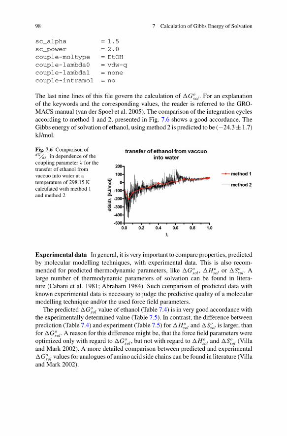
of the keywords and the corresponding values, the reader is referred to the GRO-MACS manual (van der Spoel et al. 2005). The comparison of the integration cyclesaccording to method 1 and 2, presented in Fig. 7.6 shows a good accordance. TheGibbs energy of solvation of ethanol, using method 2 is predicted to be (−24.3 ± 1.7)kJ/mol.
Fig. 7.6 Comparison ofdG�dλ in dependence of thecoupling parameter λ for thetransfer of ethanol fromvaccuo into water at atemperature of 298.15 Kcalculated with method 1and method 2
Experimental data In general, it is very important to compare properties, predictedby molecular modelling techniques, with experimental data. This is also recom-mended for predicted thermodynamic parameters, like �Go
sol , �Hosol or �So
sol . Alarge number of thermodynamic parameters of solvation can be found in litera-ture (Cabani et al. 1981; Abraham 1984). Such comparison of predicted data withknown experimental data is necessary to judge the predictive quality of a molecularmodelling technique and/or the used force field parameters.
The predicted �Gosol value of ethanol (Table 7.4) is in very good accordance with
the experimentally determined value (Table 7.5). In contrast, the difference betweenprediction (Table 7.4) and experiment (Table 7.5) for �Ho
sol and �Sosol is larger, than
for �Gosol . A reason for this difference might be, that the force field parameters were
optimized only with regard to �Gosol , but not with regard to �Ho
sol and �Sosol (Villa
and Mark 2002). A more detailed comparison between predicted and experimental�Go
sol values for analogues of amino acid side chains can be found in literature (Villaand Mark 2002).
7.2 Examples – Conceptual and Practical Considerations 99
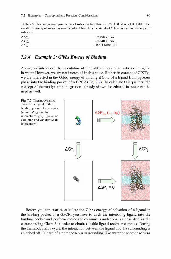
Table 7.5 Thermodynamic parameters of solvation for ethanol at 25 ◦C (Cabani et al. 1981). Thestandard entropy of solvation was calculated based on the standard Gibbs energy and enthalpy ofsolvation
�Gosol −20.98 kJ/mol
�Hosol −52.40 kJ/mol
�Sosol −105.4 J/(mol K)
7.2.4 Example 2: Gibbs Energy of Binding
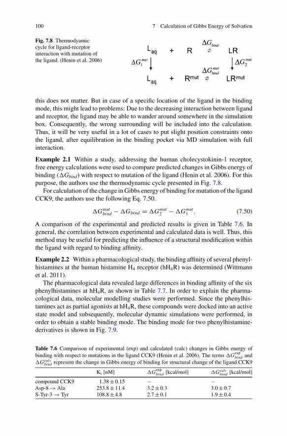
Above, we introduced the calculation of the Gibbs energy of solvation of a ligandin water. However, we are not interested in this value. Rather, in context of GPCRs,we are interested in the Gibbs energy of binding �Gbind of a ligand from aqueousphase into the binding pocket of a GPCR (Fig. 7.7). To calculate this quantity, theconcept of thermodynamic integration, already shown for ethanol in water can beused as well.
Fig. 7.7 Thermodynamiccycle for a ligand in thebinding pocket of a receptor(coloured ligand: fullinteractions; grey ligand: noCoulomb and van der Waalsinteractions)
Before you can start to calculate the Gibbs energy of solvation of a ligand inthe binding pocket of a GPCR, you have to dock the interesting ligand into thebinding pocket and perform molecular dynamic simulations, as described in thecorresponding Chap. 6 in order to obtain a stable ligand-receptor-complex. Duringthe thermodynamic cycle, the interaction between the ligand and the surrounding isswitched off. In case of a homogeneous surrounding, like water or another solvens
100 7 Calculation of Gibbs Energy of Solvation
Fig. 7.8 Thermodyamiccycle for ligand-receptorinteraction with mutation ofthe ligand. (Henin et al. 2006)
this does not matter. But in case of a specific location of the ligand in the bindingmode, this might lead to problems: Due to the decreasing interaction between ligandand receptor, the ligand may be able to wander around somewhere in the simulationbox. Consequently, the wrong surrounding will be included into the calculation.Thus, it will be very useful in a lot of cases to put slight position constraints ontothe ligand, after equilibration in the binding pocket via MD simulation with fullinteraction.
Example 2.1 Within a study, addressing the human cholecystokinin-1 receptor,free energy calculations were used to compare predicted changes in Gibbs energy ofbinding (�Gbind) with respect to mutation of the ligand (Henin et al. 2006). For thispurpose, the authors use the thermodynamic cycle presented in Fig. 7.8.
For calculation of the change in Gibbs energy of binding for mutation of the ligandCCK9, the authors use the following Eq. 7.50.
�Gmutbind − �Gbind = �Gmut
2 − �Gmut1 . (7.50)
A comparison of the experimental and predicted results is given in Table 7.6. Ingeneral, the correlation between experimental and calculated data is well. Thus, thismethod may be useful for predicting the influence of a structural modification withinthe ligand with regard to binding affinity.
Example 2.2 Within a pharmacological study, the binding affinity of several phenyl-histamines at the human histamine H4 receptor (hH4R) was determined (Wittmannet al. 2011).
The pharmacological data revealed large differences in binding affinity of the sixphenylhistamines at hH4R, as shown in Table 7.7. In order to explain the pharma-cological data, molecular modelling studies were performed. Since the phenylhis-tamines act as partial agonists at hH4R, these compounds were docked into an activestate model and subsequently, molecular dynamic simulations were performed, inorder to obtain a stable binding mode. The binding mode for two phenylhistamine-derivatives is shown in Fig. 7.9.
Table 7.6 Comparison of experimental (exp) and calculated (calc) changes in Gibbs energy ofbinding with respect to mutations in the ligand CCK9 (Henin et al. 2006). The terms �G
expbind and
�Gcalcbind represent the change in Gibbs energy of binding for structural change of the ligand CCK9
Ki [nM] �Gexpbind [kcal/mol] �Gcalc
bind [kcal/mol]
compound CCK9 1.38 ± 0.15 − −Asp-8 → Ala 253.8 ± 11.4 3.2 ± 0.3 3.0 ± 0.7S-Tyr-3 → Tyr 108.8 ± 4.8 2.7 ± 0.1 1.9 ± 0.4

7.2 Examples – Conceptual and Practical Considerations 101
Table 7.7 Binding affinities (pKi) of six phenylhistamine derivatives at hH4R at a temperature of298.15 K. (Wittmann et al. 2011)
R1 R2 pKi (hH4R)
PheHIS-1 H H 4.79 ± 0.04PheHIS-2 CF3 H 5.91 ± 0.12PheHIS-3 Br H 5.76 ± 0.01PheHIS-4 H CH3 6.13 ± 0.08PheHIS-5 CF3 CH3 6.80 ± 0.04PheHIS-6 Br CH3 6.56 ± 0.06
Fig. 7.9 Binding mode of two phenylhistamine derivatives PH-1 (left) and PH-5 (right) in thebinding pocket of hH4R. (Wittmann et al. 2011, copyright by Springer, with permission fromSpringer)
In case, that the small phenylhistamine (R1 = R2 = H) is bound to the receptor, twosmall empty pockets (Fig. 7.9, left: arrow 1 and arrow 2) were identified. If a morebulkier phenylhistamine (R1 = CF3, R2 = CH3) is bound to the receptor, the methylmoiety (CH3) fits well into pocket 1 (Fig. 7.9, right: arrow 1) and the trifluoromethylmoiety (CF3) fits well into pocket 2 (Fig. 7.9, right: arrow 2). Thus, it can besuggested that the additional methyl and trifluoromethyl moieties result in an increaseof interaction between the hH4R and ligand. This is in good accordance to higheraffinity of PH-5 compared to PH-1 (Table 7.7). However, using the thermodynamicintegration method, this qualitative explanation could be quantified (Table 7.8).
A correlation of the experimentally determined pKi values with the predictedchanges in Gibbs energy of solvation for the transfer of the ligands from aqueousphase into the binding pocket of hH4R is presented in Fig. 7.10.
As revealed by Fig. 7.10, the correlation between predicted and experimental datais quite well. In this case, there is rather no difference, if the predicted ��Go
sol valuefor the transfer of the ligand from aqueous phase in to binding pocket of hH4R, or thepredicted �Go
sol value of the ligand in the binding pocket of hH4R is correlated withthe experimentally determined pKi value. However, the more accurate way would be
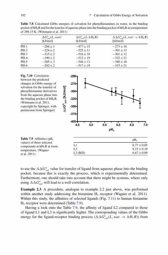
102 7 Calculation of Gibbs Energy of Solvation
Table 7.8 Calculated Gibbs energies of solvation for phenylhistamines in water, in the bindingpocket of hH4R and for the transfer of aqueous phase into the binding pocket of hH4R at a temperatureof 298.15 K. (Wittmann et al. 2011)
�Gosol(L, wat) �Go
sol(L, hH4R) ��Gosol(L, wat → hH4R)
[kJ/mol] [kJ/mol] [kJ/mol]
PH-1 −204 ± 1 −477 ± 15 −273 ± 16PH-2 −224 ± 2 −525 ± 11 −301 ± 13PH-3 −215 ± 2 −516 ± 10 −301 ± 12PH-4 −190 ± 2 −512 ± 19 −322 ± 21PH-5 −205 ± 3 −544 ± 13 −340 ± 16PH-6 −202 ± 2 −517 ± 19 −315 ± 21
Fig. 7.10 Correlationbetween the predictedchanges in Gibbs energy ofsolvation for the transfer ofphenylhistamine derivativesfrom the aqueous phase intothe binding pocket of hH4R.(Wittmann et al. 2011,copyright by Springer, withpermission from Springer)
Table 7.9 Affinities (pKi
values) of three selectedcompounds at hH1R at roomtemperature. (Wagneret al. 2011)
pKi
L1 6.77 ± 0.05L2 8.15 ± 0.10L3 (R/S) 6.67 ± 0.09
to use the ��Gosol value for transfer of ligand from aqueous phase into the binding
pocket, because this is exactly the process, which is experimentally determined.Furthermore, one should take into account that there might be systems, where onlyusing ��Go
sol will lead to a well correlation.
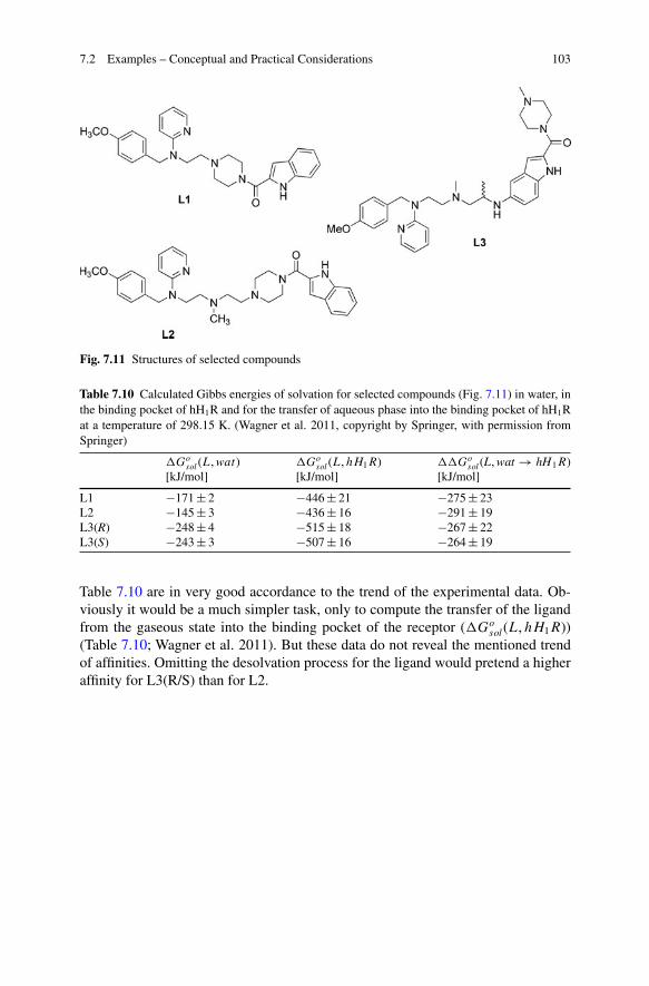
Example 2.3 A procedure, analogue to example 2.2 just above, was performedwithin another study addressing the histamine H1 receptor (Wagner et al. 2011).Within this study, the affinities of selected ligands (Fig. 7.11) to human histamineH1 receptor were determined (Table 7.9).
Having a look onto the Table 7.9, the affinity of ligand L2 compared to thoseof ligand L1 and L3 is significantly higher. The corresponding values of the Gibbsenergy for the ligand-receptor binding process (��Go
sol(L, wat → hH1R)) from
7.2 Examples – Conceptual and Practical Considerations 103
Fig. 7.11 Structures of selected compounds
Table 7.10 Calculated Gibbs energies of solvation for selected compounds (Fig. 7.11) in water, inthe binding pocket of hH1R and for the transfer of aqueous phase into the binding pocket of hH1Rat a temperature of 298.15 K. (Wagner et al. 2011, copyright by Springer, with permission fromSpringer)
�Gosol(L, wat) �Go
sol(L, hH1R) ��Gosol(L, wat → hH1R)
[kJ/mol] [kJ/mol] [kJ/mol]
L1 −171 ± 2 −446 ± 21 −275 ± 23L2 −145 ± 3 −436 ± 16 −291 ± 19L3(R) −248 ± 4 −515 ± 18 −267 ± 22L3(S) −243 ± 3 −507 ± 16 −264 ± 19
Table 7.10 are in very good accordance to the trend of the experimental data. Ob-viously it would be a much simpler task, only to compute the transfer of the ligandfrom the gaseous state into the binding pocket of the receptor (�Go
sol(L, hH1R))(Table 7.10; Wagner et al. 2011). But these data do not reveal the mentioned trendof affinities. Omitting the desolvation process for the ligand would pretend a higheraffinity for L3(R/S) than for L2.