Modelling of Defects DFT and complementary methods

Tor Svendsen BjørheimPhD fellow, FERMiO, Department of Chemistry

University of Oslo

NorFERM-2008, 3rd -7th of October 2008

Outline Background / Introduction DFT

Theory DFT calculations in practice Case studies

Supplementary Methods Nudged Elastic Band Molecular Dynamics Monte Carlo approach

Summary

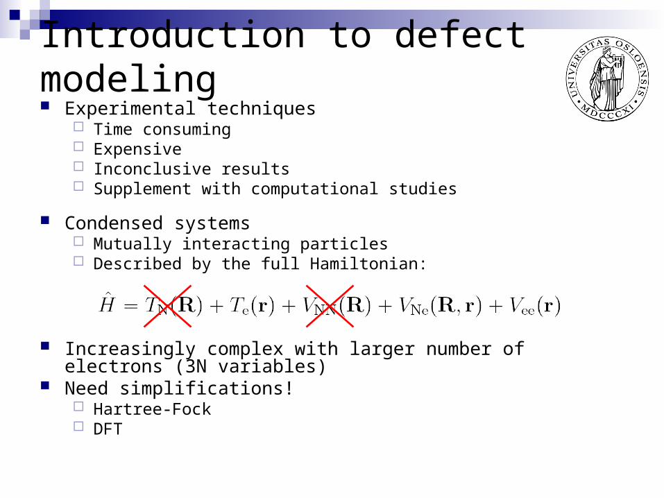
Introduction to defect modeling Experimental techniques

Time consuming Expensive Inconclusive results Supplement with computational studies

Condensed systems Mutually interacting particles Described by the full Hamiltonian:

Increasingly complex with larger number of electrons (3N variables) Need simplifications!

Hartree-Fock DFT

DFT -

Density Functional

Theory

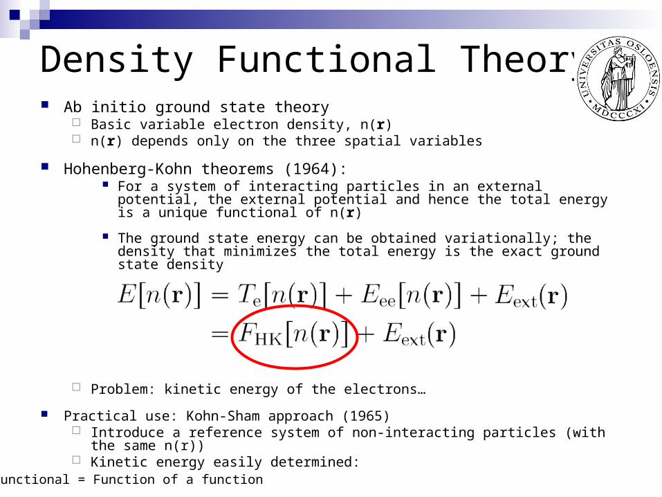
Density Functional Theory Ab initio ground state theory

Basic variable electron density, n(r) n(r) depends only on the three spatial variables

Hohenberg-Kohn theorems (1964): For a system of interacting particles in an external potential, the external

potential and hence the total energy is a unique functional of n(r)

The ground state energy can be obtained variationally; the density that minimizes the total energy is the exact ground state density

Problem: kinetic energy of the electrons…

Practical use: Kohn-Sham approach (1965) Introduce a reference system of non-interacting particles (with the same n(r)) Kinetic energy easily determined:

Functional = Function of a function

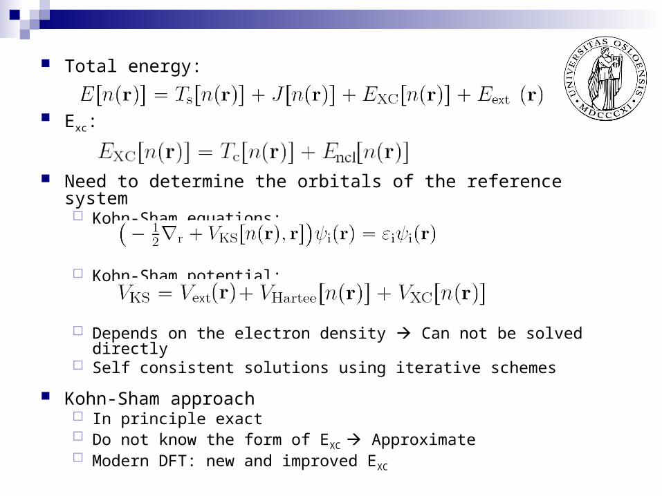
Total energy:

Exc:

Need to determine the orbitals of the reference system Kohn-Sham equations:

Kohn-Sham potential:

Depends on the electron density Can not be solved directly Self consistent solutions using iterative schemes

Kohn-Sham approach In principle exact Do not know the form of EXC Approximate Modern DFT: new and improved EXC

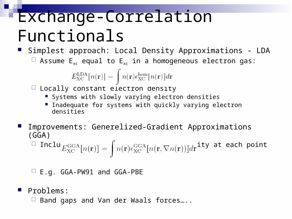
Simplest approach: Local Density Approximations - LDA Assume Exc equal to Exc in a homogeneous electron gas:

Locally constant electron density Systems with slowly varying electron densities Inadequate for systems with quickly varying electron densities

Improvements: Generelized-Gradient Approximations (GGA) Include gradients of the electron density at each point

E.g. GGA-PW91 and GGA-PBE

Problems: Band gaps and Van der Waals forces…..

Exchange-Correlation Functionals

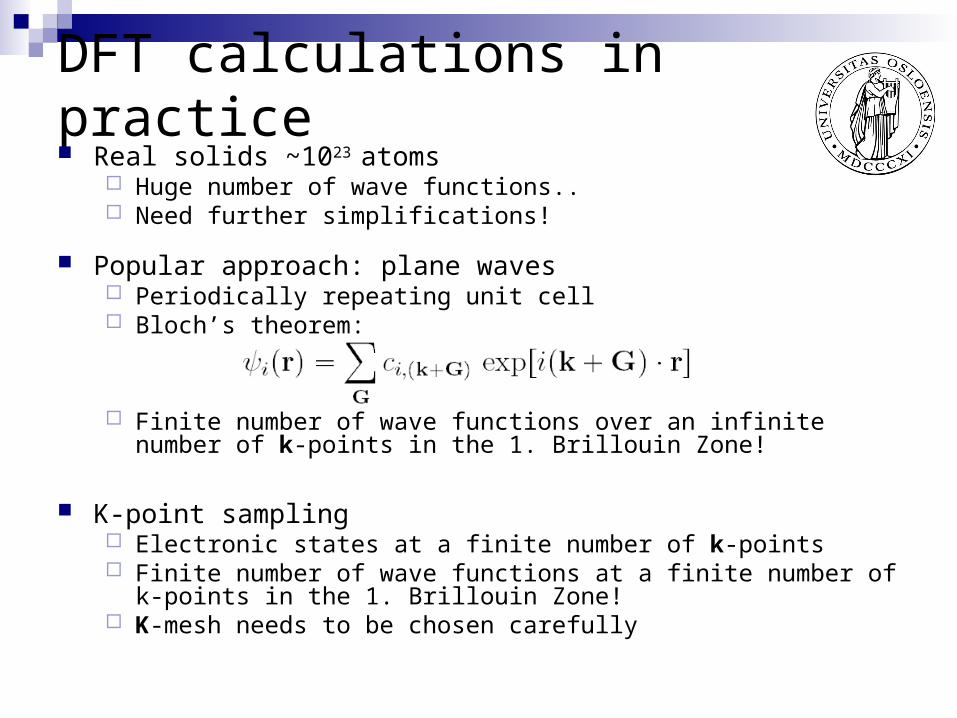
DFT calculations in practice Real solids ~1023 atoms

Huge number of wave functions.. Need further simplifications!

Popular approach: plane waves Periodically repeating unit cell Bloch’s theorem:

Finite number of wave functions over an infinite number of k-points in the 1. Brillouin Zone!

K-point sampling Electronic states at a finite number of k-points Finite number of wave functions at a finite number of k-points in the 1.

Brillouin Zone! K-mesh needs to be chosen carefully

Defects in solids

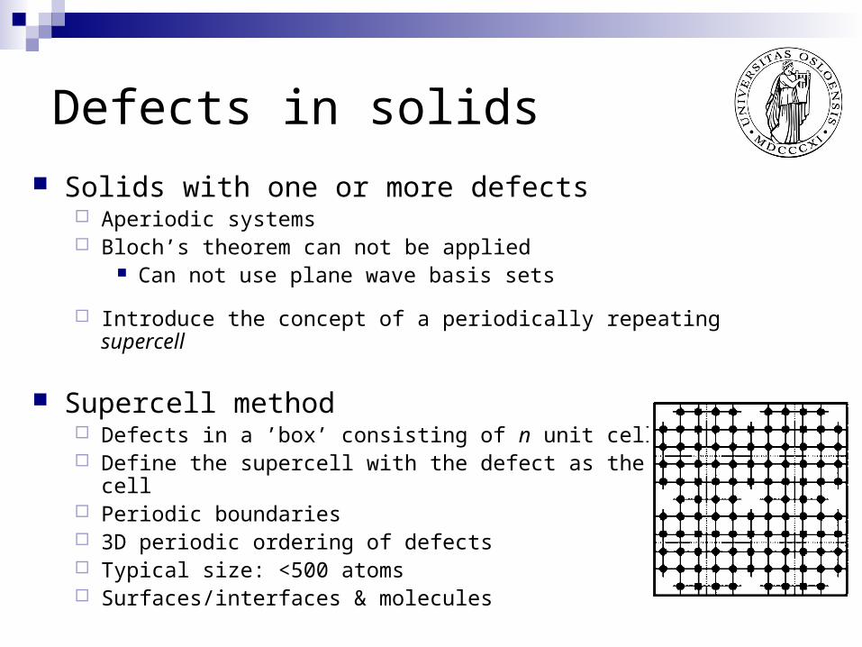
Solids with one or more defects Aperiodic systems Bloch’s theorem can not be applied

Can not use plane wave basis sets

Introduce the concept of a periodically repeating supercell

Supercell method Defects in a ’box’ consisting of n unit cells Define the supercell with the defect as the new unit cell Periodic boundaries 3D periodic ordering of defects Typical size: <500 atoms Surfaces/interfaces & molecules

Finite-Cluster approach Defects in finite atomic clusters No interaction with defects in neighboring unit cells Avoid surface effects: large clusters

Green’s Function Embedding Technique Purely mathematical Defect regions embedded in known DFT Green’s

function of bulk Ideal for studies of isolated defects (in theory) Numerically challenging…..

Alternative approaches

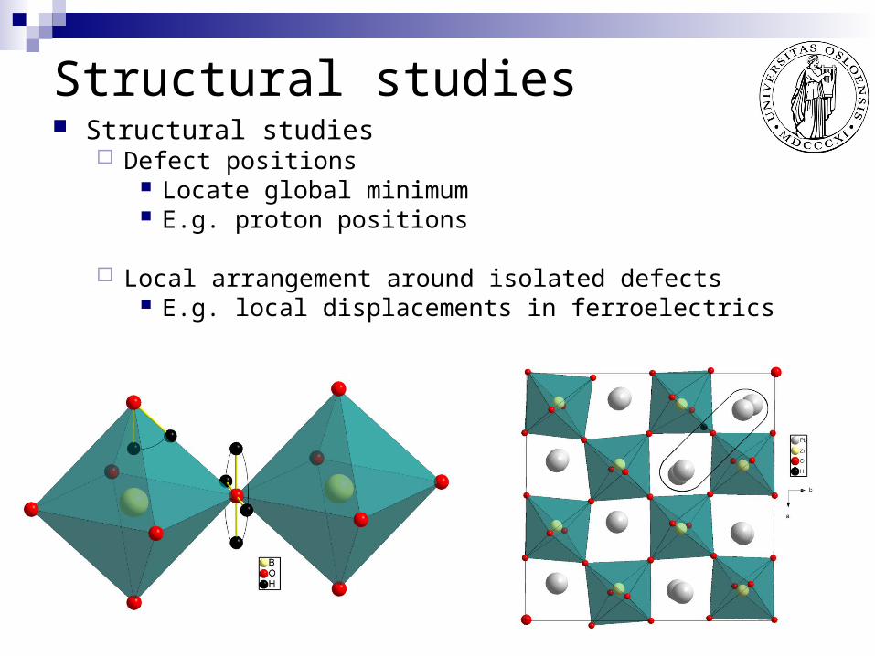
Structural studies Structural studies

Defect positions Locate global minimum E.g. proton positions

Local arrangement around isolated defects E.g. local displacements in ferroelectrics

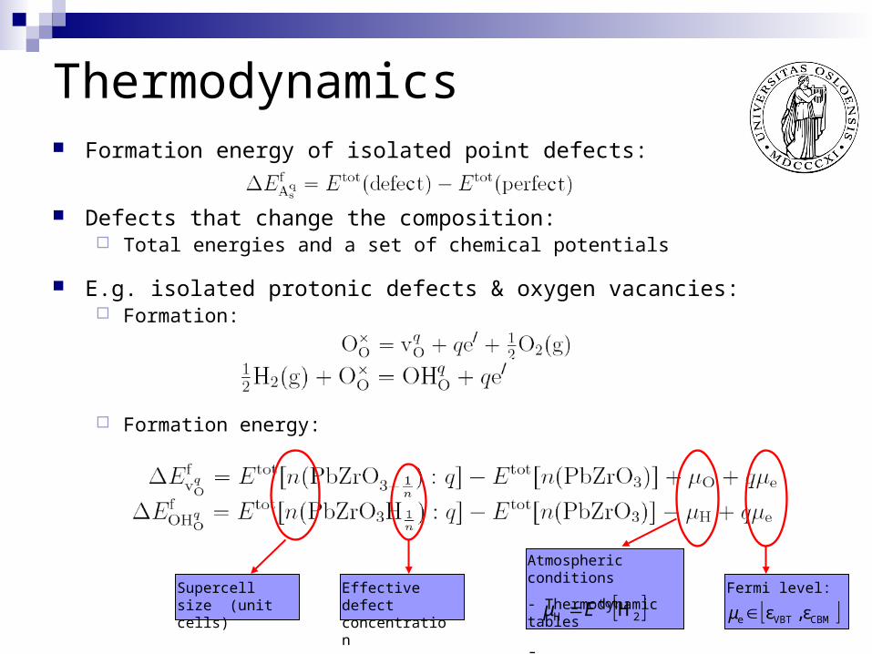
Thermodynamics Formation energy of isolated point defects:

Defects that change the composition: Total energies and a set of chemical potentials

E.g. isolated protonic defects & oxygen vacancies: Formation:

Formation energy:

Effective defect concentration

Supercell size (unit cells)

Atmospheric conditions

- Thermodynamic tables

-

Fermi level:

CBMVBTe ε,εμ 2tot

H HEμ

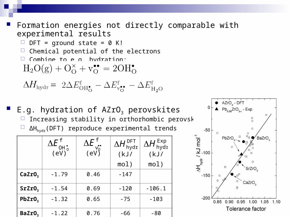
Formation energies not directly comparable with experimental results DFT = ground state = 0 K! Chemical potential of the electrons Combine to e.g. hydration:

E.g. hydration of AZrO3 perovskites Increasing stability in orthorhombic perovskites ∆Hhydr(DFT) reproduce experimental trends

f

vOEf

OHOE

(eV) (eV) (kJ/mol) (kJ/mol)

CaZrO3 -1.79 0.46 -147

SrZrO3 -1.54 0.69 -120 -106.1

PbZrO3 -1.32 0.65 -75 -103

BaZrO3 -1.22 0.76 -66 -80

DFThydrH Exp

hydrH

Defect levels Defect levels

Transition between charge states: Ef(q/q’) Experimentally: DLTS Determine the preferred charge state of defects

In supercell calculations: Determine ΔEf for all charge states ΔEf for all Fermi level positions Most stable: charge state with lowest ΔEf

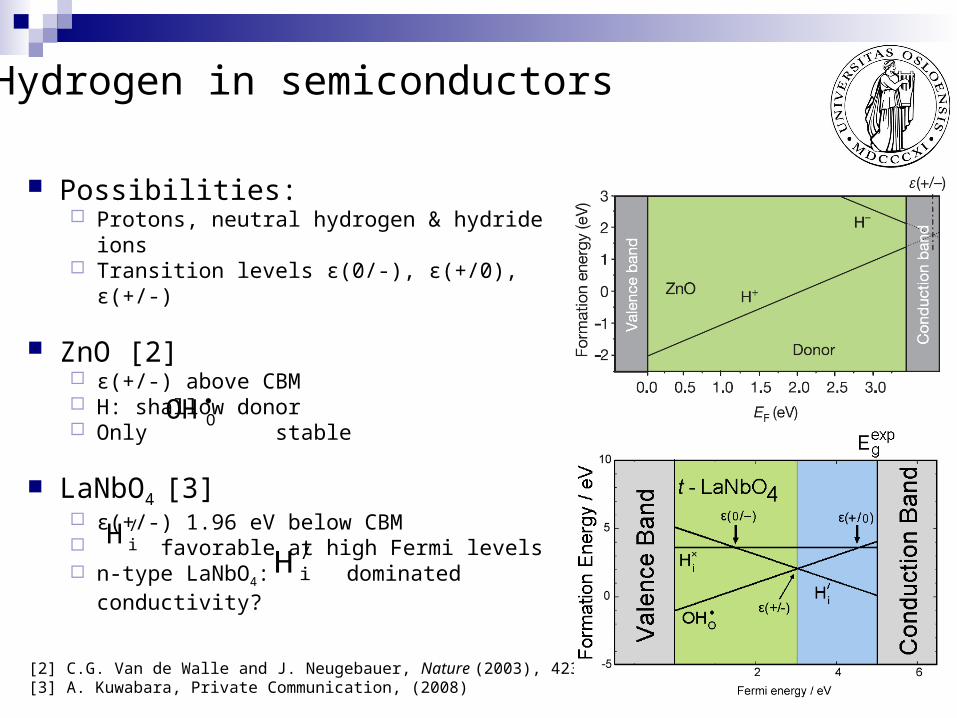
Possibilities: Protons, neutral hydrogen & hydride ions Transition levels ε(0/-), ε(+/0), ε(+/-)

ZnO [2] ε(+/-) above CBM H: shallow donor Only stable

LaNbO4 [3] ε(+/-) 1.96 eV below CBM favorable at high Fermi levels n-type LaNbO4: dominated

conductivity?

/iH

[2] C.G. Van de Walle and J. Neugebauer, Nature (2003), 423[3] A. Kuwabara, Private Communication, (2008)

OOH

/iH

Hydrogen in semiconductors

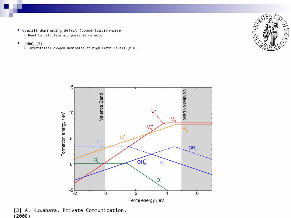
Overall dominating defect (concentration-wise) Need to calculate all possible defects

LaNbO4 [3] Interstitial oxygen dominates at high Fermi levels (0 K!)

[3] A. Kuwabara, Private Communication, (2008)

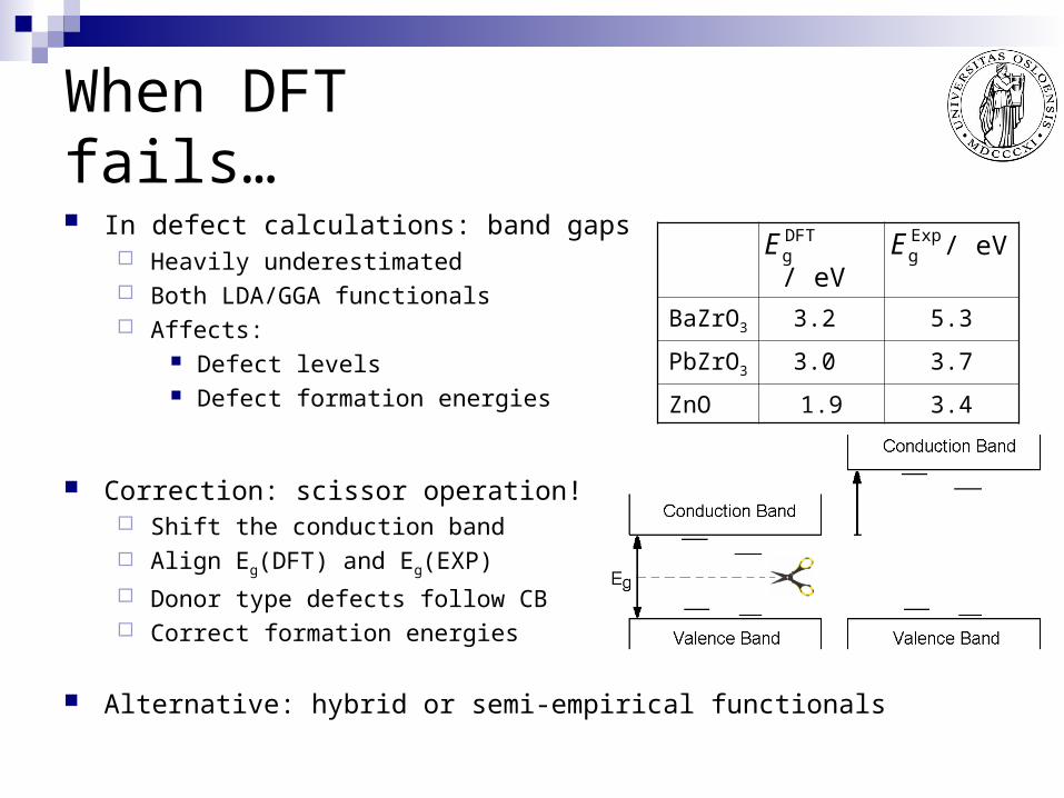
When DFT fails… In defect calculations: band gaps

Heavily underestimated Both LDA/GGA functionals Affects:

Defect levels Defect formation energies

Correction: scissor operation! Shift the conduction band Align Eg(DFT) and Eg(EXP)

Donor type defects follow CB Correct formation energies

Alternative: hybrid or semi-empirical functionals

/ eV / eV

BaZrO3 3.2 5.3

PbZrO3 3.0 3.7

ZnO 1.9 3.4

DFTgE

ExpgE

Complementary methods

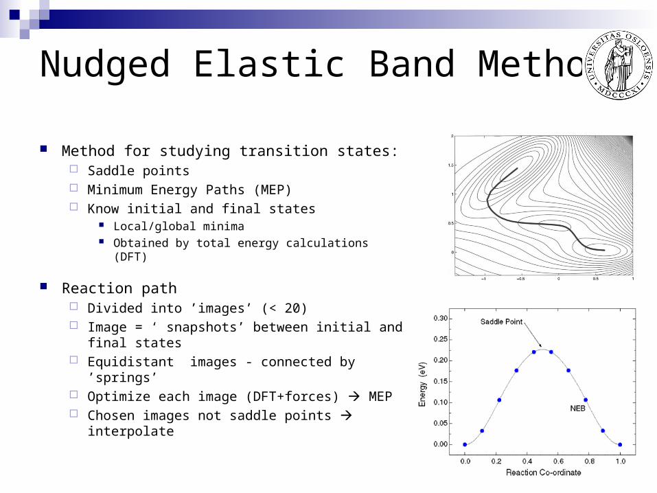
Nudged Elastic Band Method

Method for studying transition states: Saddle points Minimum Energy Paths (MEP) Know initial and final states

Local/global minima Obtained by total energy calculations (DFT)

Reaction path Divided into ’images’ (< 20) Image = ‘ snapshots’ between initial and final

states Equidistant images - connected by ’springs’ Optimize each image (DFT+forces) MEP Chosen images not saddle points interpolate

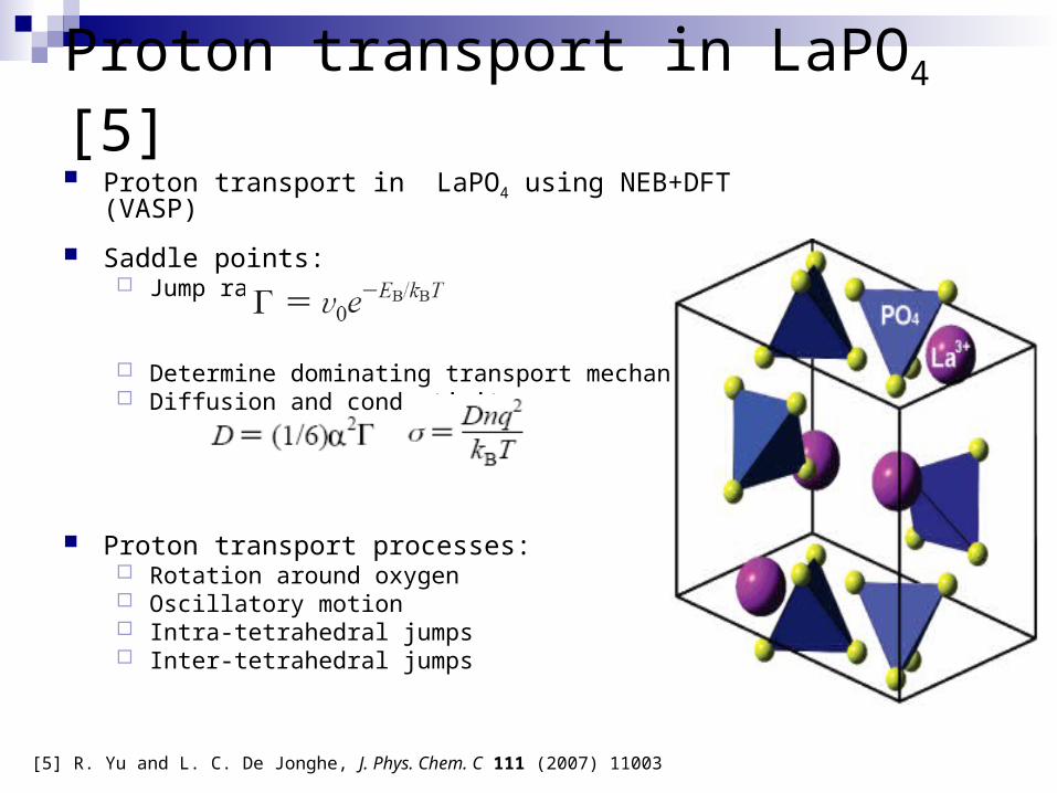
Proton transport in LaPO4 [5] Proton transport in LaPO4 using NEB+DFT (VASP)

Saddle points: Jump rates:

Determine dominating transport mechanism Diffusion and conductivity:

Proton transport processes: Rotation around oxygen Oscillatory motion Intra-tetrahedral jumps Inter-tetrahedral jumps

[5] R. Yu and L. C. De Jonghe, J. Phys. Chem. C 111 (2007) 11003

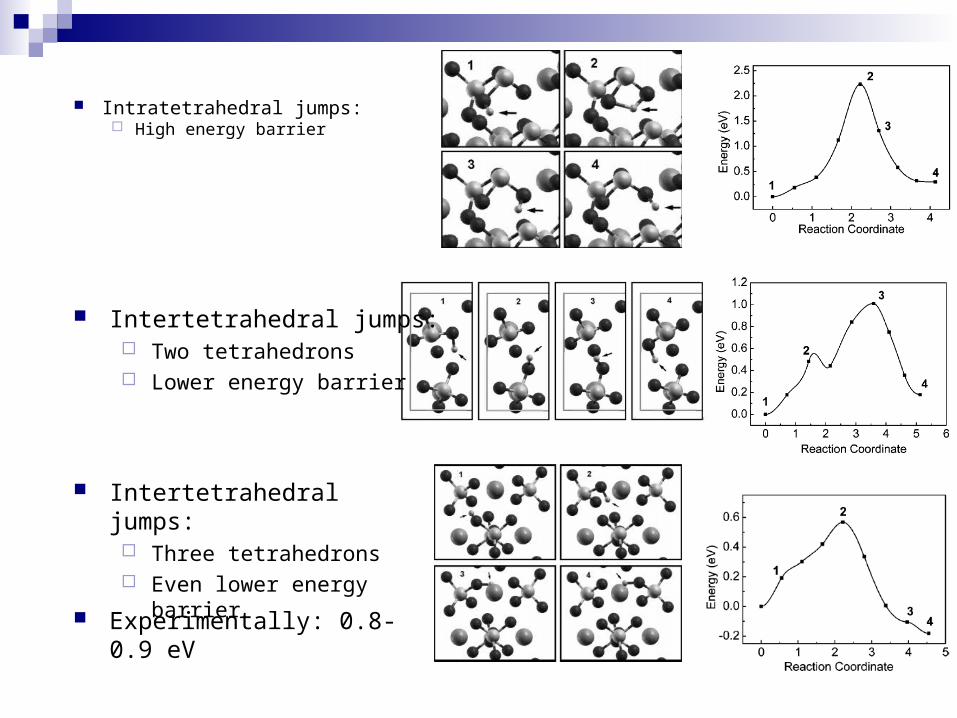
Intratetrahedral jumps: High energy barrier

Intertetrahedral jumps: Two tetrahedrons Lower energy barrier

Intertetrahedral jumps: Three tetrahedrons Even lower energy barrier

Experimentally: 0.8-0.9 eV

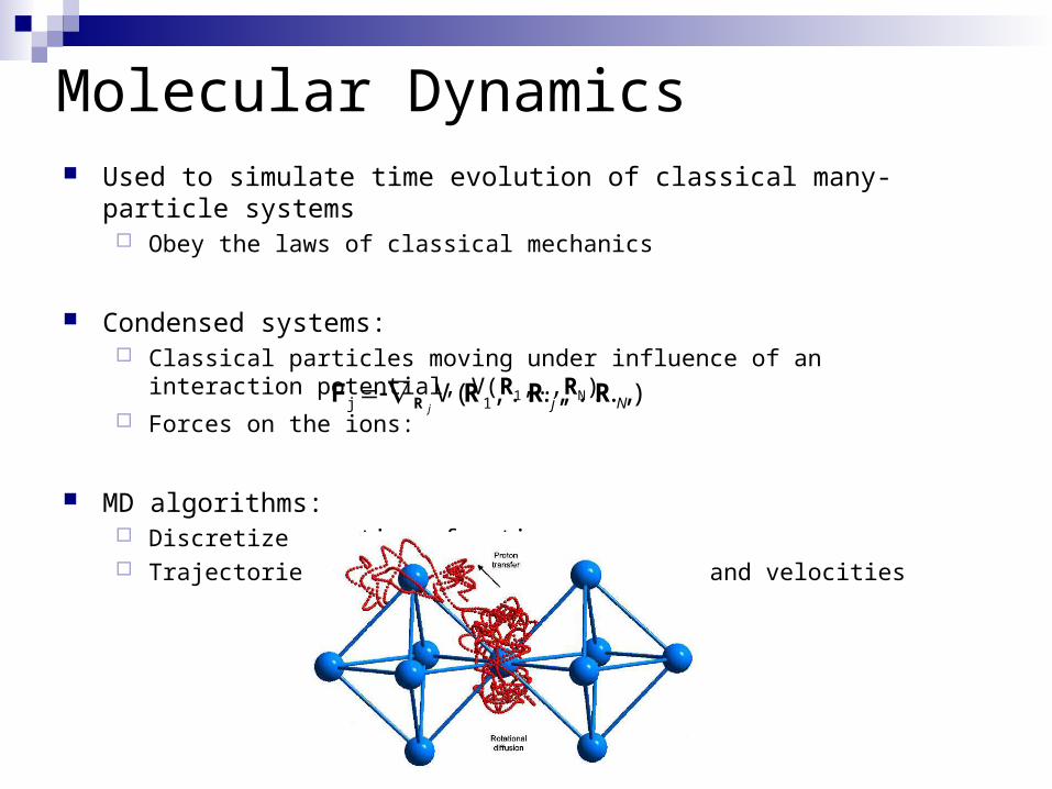
Molecular Dynamics Used to simulate time evolution of classical many-particle systems

Obey the laws of classical mechanics

Condensed systems: Classical particles moving under influence of an interaction potential, V(R1,…,RN)

Forces on the ions:

MD algorithms: Discretize equation of motion Trajectories: stepwise update positions and velocities

),...,,...,(V 1j NjjRRRF R

Interionic interactions: Model potential vs. first-principles

Model potential Parameterized to fit experimental or first principles data Advantages

Possible to treat large systems Long time evolution

Disadvantages Inaccurate potentials Poor force representation

First-principles First-principles electronic structure calculation (e.g. DFT) at each ionic step Advantages:

Accurate forces Realistic dynamic description

Disadvatages Computationally demanding Small systems (~100 ions) Short time periods (~ps)

Good statistical accuracy

Poor statistical accuracy..

Monte-Carlo approach Loosely described:

Statistical simulation methods

Conventional methods (MD): Discretize equations describing the physical process E.g. equations of motion

Monte-Carlo approach Simulate the physical process directly No need to solve the underlying equations Requirement: process described by probability distribution functions (PDF) Average results over the number of observations

Proton diffusion Jump frequency and PDF:

N

nmmP

1n/ TEii Bia0 k/exp

Summary

Many different computational approaches

Systematic trends

Fundamental processes

Predict defect properties of real materials

Combine different methods

Acknowledgements

Akihide Kuwabara

Espen Flage-Larsen

Svein Stølen

Truls Norby

Colleagues at the Solid State Electrochemistry group in Oslo

Thank You !!

Thank You!