Embed Size (px)
Citation preview

Modelling of
Contact and Friction in
Deep Drawing Processes
Andr�e Westeneng
This research project was sponsored by Corus and Quaker Chemical B.V. It wascarried out at the University of Twente.
ISBN: 90-365-1549-1
Printed by FEBO druk B.V., Enschede
Copyright c 2001 by J.D. Westeneng. Enschede
MODELLING OF CONTACT AND FRICTION IN DEEP DRAWINGPROCESSES
PROEFSCHRIFT
ter verkrijging vande graad van doctor aan de Universiteit Twente,
op gezag van de rector magni�cus,prof.dr. F.A. van Vught,
volgens besluit van het College voor Promotiesin het openbaar te verdedigen
op vrijdag 23 maart 2001 te 15.00 uur.
door
Jan Dirk Westeneng
geboren op 30 juli 1972te Woudenberg

Dit proefschrift is goedgekeurd door:
Promotor: prof.ir. A.W.J. de GeeAssistent-promotor: dr.ir. D.J. Schipper
Acknowledgements
This project is �nancially supported by Corus and Quaker Chemical B.V. Forthis support and for the many useful discussions during the \FRIS"-meetingsand practical assistance during the 4 years, I want to thank Wilko Emmens,Rudi ter Haar and Hans Holtkamp of Corus and Nico Broekhof, Jan Melsen andHenk Mulder of Quaker Chemical B.V.
Also many thanks to my supervisor and assistent-promotor Dik Schipper forthe many discussions and suggestions regarding the research. He supported mevery well during the promotion work. Prof.ir. A.W.J. de Gee is thanked for beingmy promotor.
Thanks to the other members of the graduation committee: Prof. dr. ir. H.J. Grootenboer, Prof. dr. ir. F.J.A.M. van Houten, Prof. dr. ir. J. Hu�etink andProf. dr. ir. M. Vermeulen.
For performing an adeaquate job, it is always important to have a nice atmo-sphere in the group. Especially, the co�ee breaks oftenly served with cake and thefriday-late-afternoon drinking events served as a good opportunity to socialize.Regularly playing table tennis, tennis and squash with some colleagues nulli�edthe e�ect of these events on my condition and gave me fun. I want to thank thefollowing (ex-)members of the Tribology group: Ton de Gee, Johan Ligterink,Hans Moes, Wijtze ten Napel, Matthijn de Rooij, Dik Schipper, Kees Venner,Laurens de Boer, Willy Kerver, Walter Lette, Erik de Vries, Bernd Brogle, RobCuperus, Mark van Drogen, Edwin Gelinck, Qiang Liu, Harald Lubbinge, MarcMasen, Henk Metselaar, Elmer Mulder, Dani�el van Odyck, Patrick Pirson, JanWillem Sloetjes, Ronald van der Stegen, Harm Visscher and Ysbrand Wijnant.
For practical assistance for shorter or longer time, I want to thank the sec-retaries Belinda Bruinink, Susan Godschalk, Marieke Jansen, Carolien Post, An-nemarie Teunissen, Debbie Vrieze and Yvonne Weber.
Laurens de Boer, Willie Kerver and Erik de Vries are thanked for manufac-turing parts for experimental devices and their technical assistance during theexperiments.
Katrina Emmett improved the english language in this thesis and is thanked

vi Acknowledgements
for this job.Dani�el van Odyck and Matthijn de Rooij are thanked for being my paran-
imfs. Matthijn is also thanked for the useful suggestions and discussions duringmy promotion time.
At last but not at least, my family, friends and former roommates at the Fazantstraatare thanked for supporting me during my promotion.
Samenvatting
Wrijving speelt bij plaatomvormingsprocessen als dieptrekken een belangrijkerol. Samen met de deformatie van het plaatmateriaal, bepaalt de wrijving de televeren stempel- en plooihouderkracht. Daardoor heeft zij bij dun plaatmateriaaleen grote invloed op de voor deformatie benodigde energie. Daarnaast heeftde wrijving een invloed op de spanningen en de rekken in het plaatmaterial enhierdoor op de kwaliteit van een diep te trekken produkt. Daarom is het vanbelang de wrijving tussen het gereedschap en het werkstuk te controleren.
Het is bekend dat wrijving bij gesmeerde contacten geen constante is maarvarieert als functie van bijvoorbeeld de dieptreksnelheid, als beschreven doorde Stribeck curve. Hierbij zijn (Elastische) Hydrodynamische Smering (EHL),Gemengde Smering (ML) en Grenssmering (BL) de mogelijke smeringsregimes.Uit de literatuur is bekend dat bij dieptrekprocessen grenssmering gecombineerdmet ploegen van gereedsschapsruwheidstoppen door het plaatmateriaal, in ditproefschrift aangeduid met BL&P, een veel voorkomend en belangrijk wrijv-ingsmechanisme is. De wrijvingsco�eÆci�ent in het BL&P regime wordt vaak con-stant verondersteld, maar metingen wijzen uit dat bij plaatomvormingsprocessenverscheidene parameters de wrijvingsco�eÆci�ent bepalen. De wrijving die optreedtin dit regime is in de literatuur nauwelijks gemodeleerd en daarom wordt in ditproefschrift een nieuw wrijvingsmodel gepresenteerd.
Een literatuur overzicht wordt gegeven, betre�ende de wrijving van grensla-gen, geadsorbeerd aan glijdende oppervlakken. In dit overzicht wordt aangetoonddat de wrijving van grenslagen afhankelijk is van de chemische structuur van delagen, de glijsnelheid, de temperatuur, de dikte van de lagen en de aangebrachtenormaaldruk.
Vervolgens wordt er een contactmodel ontwikkeld voor (ideaal) plastisch de-formerende plaatruwheden. Dit contactmodel voorspelt het waar contactopper-vlak van het plaatmateriaal dat nodig is voor het wrijvingsmodel. Resultatenvan berekeningen met het contactmodel laten zien dat het waar contactopper-vlak niet-lineair toeneemt met de nominale druk. Voor hoge drukken neemt hetminder dan evenredig toe met de nominale druk, terwijl voor lage drukken deafplatting sterk afhankelijk is van de ruwheidshoogte verdeling van het plaat-materiaal. De hardheid van het plaatmateriaal speelt eveneens een rol in het
viii Samenvatting
afplattingsproces.Een apparaat is gebouwd waarmee de topogra�e van een zacht ruw werkstuk-
materiaal in contact met een glazen stempel in situ kan worden gemeten ondersimultane werking van een normaalkracht en een trekbelasting. De resultatenvan experimenten waarin alleen een normaalkracht is aangebracht, laten zien datde experimentele waarden van het waar contactoppervlak goed worden voorspelddoor het contactmodel. Er is een verband gevonden tussen de afplating en dedikte van het plaatmateriaal. Bulkrek heeft eveneens een grote invloed op detopogra�e van het materiaal. Wanneer gelijktijdig een normaal- en een trekbe-lasting wordt aangebracht, kan afhankelijk van de nominale druk en de dikte vanhet plaatmateriaal zowel afplatting als verruwing van het plaatmateriaal optre-den.
Gebruikmakend van het contactmodel en de sliplijnen theorie van Challen &Oxley, is een model ontwikkeld voor voorspelling van de wrijving in vlakke con-tacten onder condities van grenssmering in combinatie met ploegen. Het wrijvingsmodel voorspelt een wrijvingsco�eÆci�ent die afhankelijk is van de nominale druk,de bulkrek, de hardheid van het plaatmateriaal, de hoogteverdelingsfunctie vande ruwheden van het plaatmateriaal, ruwheidsparameters van het gereedschap enhet grenssmeermiddel. Verschillende experimenten zijn uitgevoerd om het wrijv-ingsmodel te veri��eren. De trends van de wrijvingsco�eÆci�ent als functie van deruwheid van het gereedschap en de nominale druk worden goed door het wrijv-ings model voorspeld, al is de kwantitatieve overeenkomst soms wat minder. Ditis geen verrassing, gelet op de onzekerheden in de schattingen van een aantalonbekende input parameters van het model.
Summary
In Sheet Metal Forming (SMF) processes, such as deep drawing, friction playsan important role. Together with the deformation of the sheet, the friction de-termines the required punch force and the blankholder force. Consequently, thefriction in uences the energy which is needed to deform a sheet material. Frictionalso in uences the stresses and strains in the workpiece material and, hence, thequality of the product. Therefore, it is important to control the friction betweenthe tools and the workpiece.
It is well known that for lubricated contacts the coeÆcient of friction is not aconstant, which is clearly shown by a Stribeck curve with (Elasto) HydrodynamicLubrication ((E)HL), Mixed Lubrication (ML) and Boundary Lubrication (BL)as the lubrication regimes. It is shown in the literature that BL in combinationwith Ploughing (P) of tool asperities through the workpiece is an importantfriction mechanism in deep drawing processes. Usually, the coeÆcient of frictionin the BL&P regime is assumed to be constant, but measurements reported inthe literature show that it is in fact in uenced by many parameters. The BL&Pregime is not adequately modelled in the literature and, hence, a new frictionmodel is presented in this thesis.
A review is presented concerning friction between sliding surfaces with ad-sorbed boundary layers. It is shown that the friction between boundary layersdepends on the chemical structure of the layer, the sliding velocity, the temper-ature, the thickness of the layers and the applied pressure.
A contact model is derived assuming plastic deformation of the workpieceasperities. This contact model is used to obtain the real contact area of the sheetmaterial, necessary for the friction model. Results of calculations show that thereal contact area is not linearly proportional to the nominal pressure. For largepressures the real contact area increases less than proportionally with the nominalpressure, while for low pressures the real contact area is strongly dependent onthe height distribution of the surface asperities. The hardness of the workpiecealso in uences how it reacts to attening.
A test device is developed to measure the topography of a workpiece surfaceduring simultaneous normal and tensile loading. Performing static normal loadingmeasurements, the real contact area agrees rather well with the predicted values.
x Summary
A relation was found between the amount of attening and the thickness ofthe workpiece material. Bulk stretching also in uences the topography of theworkpiece. When simultaneous normal loading and stretching are applied, theworkpiece surface may be attened or roughened, depending on the thickness ofthe material and the applied nominal pressure.
Using the contact model, a friction model for at contacts is developed. ThecoeÆcient of friction appears to be dependent on the nominal pressure, the bulkstrain, the hardness and the asperity height distribution of the workpiece, rough-ness parameters of the tool and the boundary lubricant. In order to verify themodel, di�erent experiments have been performed. Although the trends of thecoeÆcient of friction as a function of the roughness of the tool and the nominalpressure are predicted well, the quantitative agreement is sometimes less, whichis not surprising, considering the uncertainties in the estimate of some of theinput parameters of the model.
Contents
Acknowledgements v
Samenvatting vii
Summary ix
Nomenclature xv
1 Introduction 11.1 Sheet Metal Forming (SMF) and deep drawing . . . . . . . . . . . 11.2 Friction in deep drawing . . . . . . . . . . . . . . . . . . . . . . . 3
1.2.1 Contact regions of deep drawing . . . . . . . . . . . . . . . 31.2.2 The generalized Stribeck curve . . . . . . . . . . . . . . . . 41.2.3 Boundary Lubrication and Ploughing . . . . . . . . . . . . 61.2.4 Lubrication mechanisms in deep drawing . . . . . . . . . . 6
1.3 The tribological system in deep drawing . . . . . . . . . . . . . . 71.4 The objective of this research . . . . . . . . . . . . . . . . . . . . 91.5 Overview . . . . . . . . . . . . . . . . . . . . . . . . . . . . . . . . 9
2 Boundary Lubrication and Ploughing (BL&P) - literature 112.1 Introduction . . . . . . . . . . . . . . . . . . . . . . . . . . . . . . 112.2 Boundary Lubrication (BL) . . . . . . . . . . . . . . . . . . . . . 11
2.2.1 Formation of boundary layers . . . . . . . . . . . . . . . . 122.2.1.1 Physical adsorption . . . . . . . . . . . . . . . . . 122.2.1.2 Chemical adsorption . . . . . . . . . . . . . . . . 132.2.1.3 Chemical reaction . . . . . . . . . . . . . . . . . 13
2.2.2 Friction of boundary layers . . . . . . . . . . . . . . . . . . 142.2.2.1 Experimental details . . . . . . . . . . . . . . . . 142.2.2.2 In uence of the pressure . . . . . . . . . . . . . . 152.2.2.3 In uence of the temperature . . . . . . . . . . . . 162.2.2.4 In uence of the speed . . . . . . . . . . . . . . . 162.2.2.5 In uence of the thickness of LB monolayers . . . 17
xii Contents
2.2.2.6 Combined in uence of parameters - curve �ts . . 172.3 Ploughing . . . . . . . . . . . . . . . . . . . . . . . . . . . . . . . 242.4 Modelling BL&P - the Challen and Oxley model . . . . . . . . . . 252.5 Summary . . . . . . . . . . . . . . . . . . . . . . . . . . . . . . . 30
3 A newly developed contact model 313.1 Overview of contact models . . . . . . . . . . . . . . . . . . . . . 31
3.1.1 Stochastic contact models for spherically shaped summits . 323.1.2 Numerical contact models . . . . . . . . . . . . . . . . . . 363.1.3 Contact models including bulk deformation . . . . . . . . . 363.1.4 Contact models including volume conservation . . . . . . . 37
3.2 An ideal plastic contact model . . . . . . . . . . . . . . . . . . . . 383.2.1 Derivation of the model . . . . . . . . . . . . . . . . . . . 383.2.2 Calculations with the ideal plastic contact model . . . . . 44
3.2.2.1 In uence of n . . . . . . . . . . . . . . . . . . . . 463.2.2.2 In uence of � . . . . . . . . . . . . . . . . . . . . 483.2.2.3 In uence of the height distribution functions . . . 48
3.2.3 No surface rise . . . . . . . . . . . . . . . . . . . . . . . . 523.3 A contact model including work hardening e�ects . . . . . . . . . 54
3.3.1 Derivation of the model . . . . . . . . . . . . . . . . . . . 543.3.2 Calculations with the work hardening model . . . . . . . . 58
3.3.2.1 In uence of n . . . . . . . . . . . . . . . . . . . . 593.3.2.2 In uence of � . . . . . . . . . . . . . . . . . . . . 59
3.4 A contact model including bulk strain e�ects . . . . . . . . . . . . 623.4.1 Overview of strain models . . . . . . . . . . . . . . . . . . 62
3.4.1.1 The model of Wilson & Sheu . . . . . . . . . . . 623.4.1.2 The model of Sutcli�e . . . . . . . . . . . . . . . 643.4.1.3 Calculations with strain models . . . . . . . . . . 66
3.4.2 Derivation of a new strain model . . . . . . . . . . . . . . 703.4.3 Calculations . . . . . . . . . . . . . . . . . . . . . . . . . . 73
3.5 In uence of sliding . . . . . . . . . . . . . . . . . . . . . . . . . . 773.6 Conclusions and summmary . . . . . . . . . . . . . . . . . . . . . 78
4 Experimental veri�cation of the contact model 814.1 The experimental device . . . . . . . . . . . . . . . . . . . . . . . 81
4.1.1 The normal force unit . . . . . . . . . . . . . . . . . . . . 814.1.2 The bulk tension force unit . . . . . . . . . . . . . . . . . 83
4.2 Experimental details . . . . . . . . . . . . . . . . . . . . . . . . . 844.2.1 Materials . . . . . . . . . . . . . . . . . . . . . . . . . . . 844.2.2 Data processing . . . . . . . . . . . . . . . . . . . . . . . . 844.2.3 Determination of the real contact area . . . . . . . . . . . 86
4.3 Normal load measurements . . . . . . . . . . . . . . . . . . . . . . 87
Contents xiii
4.3.1 Results . . . . . . . . . . . . . . . . . . . . . . . . . . . . . 874.3.2 Calculations . . . . . . . . . . . . . . . . . . . . . . . . . . 894.3.3 Comparison with the literature . . . . . . . . . . . . . . . 89
4.4 Stretching measurements . . . . . . . . . . . . . . . . . . . . . . . 924.4.1 Experimental procedure . . . . . . . . . . . . . . . . . . . 934.4.2 Results . . . . . . . . . . . . . . . . . . . . . . . . . . . . . 93
4.4.2.1 Free deformation . . . . . . . . . . . . . . . . . . 944.4.2.2 Free deformation followed by normal loading . . . 954.4.2.3 Simultaneous stretching and normal loading . . . 95
4.4.3 Calculations . . . . . . . . . . . . . . . . . . . . . . . . . . 1014.5 Deep drawing experiments . . . . . . . . . . . . . . . . . . . . . . 106
4.5.1 Introduction . . . . . . . . . . . . . . . . . . . . . . . . . . 1064.5.2 Results . . . . . . . . . . . . . . . . . . . . . . . . . . . . . 1064.5.3 Discussion . . . . . . . . . . . . . . . . . . . . . . . . . . . 112
4.6 Discussion of results . . . . . . . . . . . . . . . . . . . . . . . . . 1134.6.1 Normal load experiments . . . . . . . . . . . . . . . . . . . 1134.6.2 Stretching experiments . . . . . . . . . . . . . . . . . . . . 115
4.6.2.1 Free deformation of the asperities . . . . . . . . . 1154.6.2.2 Free deformation of the asperities followed by nor-
mal loading . . . . . . . . . . . . . . . . . . . . . 1164.6.2.3 Deformation of asperities during simultaneous -
stretching and normal loading . . . . . . . . . . . 1174.7 Summary . . . . . . . . . . . . . . . . . . . . . . . . . . . . . . . 117
5 A macroscopic friction model 1215.1 Overview of friction models . . . . . . . . . . . . . . . . . . . . . 1215.2 The structure of the friction model . . . . . . . . . . . . . . . . . 122
5.2.1 Step 1 - Static loading . . . . . . . . . . . . . . . . . . . . 1235.2.2 Step 2 - Sliding . . . . . . . . . . . . . . . . . . . . . . . . 123
5.3 The model . . . . . . . . . . . . . . . . . . . . . . . . . . . . . . . 1245.3.1 Assumptions . . . . . . . . . . . . . . . . . . . . . . . . . . 1245.3.2 Step 1 - static loading . . . . . . . . . . . . . . . . . . . . 1265.3.3 Step 2 - sliding . . . . . . . . . . . . . . . . . . . . . . . . 126
5.4 Calculation of friction . . . . . . . . . . . . . . . . . . . . . . . . 1285.4.1 In uence of the nominal pressure . . . . . . . . . . . . . . 1305.4.2 In uence of the hardness . . . . . . . . . . . . . . . . . . . 1315.4.3 In uence of lubricant-surface system . . . . . . . . . . . . 1325.4.4 In uence of the roughness of the tool . . . . . . . . . . . . 133
5.4.4.1 Lower bound of the model . . . . . . . . . . . . . 1345.4.4.2 Upper bound of the model . . . . . . . . . . . . . 136
5.4.5 In uence of the asperity height distribution function . . . 1375.5 In uence of the bulk strain . . . . . . . . . . . . . . . . . . . . . . 140
xiv Contents
5.6 Summary . . . . . . . . . . . . . . . . . . . . . . . . . . . . . . . 142
6 Experimental validation of the friction model 1456.1 Experimental devices . . . . . . . . . . . . . . . . . . . . . . . . . 145
6.1.1 The RON-tester . . . . . . . . . . . . . . . . . . . . . . . . 1456.1.2 The S-tribometer . . . . . . . . . . . . . . . . . . . . . . . 146
6.2 Materials speci�cations . . . . . . . . . . . . . . . . . . . . . . . . 1486.2.1 Workpiece materials . . . . . . . . . . . . . . . . . . . . . 1486.2.2 Tool materials . . . . . . . . . . . . . . . . . . . . . . . . . 1486.2.3 Lubricants . . . . . . . . . . . . . . . . . . . . . . . . . . . 149
6.3 Experimental procedures . . . . . . . . . . . . . . . . . . . . . . . 1506.3.1 RON-tester . . . . . . . . . . . . . . . . . . . . . . . . . . 1506.3.2 S-tribometer . . . . . . . . . . . . . . . . . . . . . . . . . . 151
6.4 E�ect of the roughness of the tool . . . . . . . . . . . . . . . . . . 1516.4.1 Experimental results . . . . . . . . . . . . . . . . . . . . . 1516.4.2 Theoretical results . . . . . . . . . . . . . . . . . . . . . . 152
6.5 E�ect of the nominal pressure . . . . . . . . . . . . . . . . . . . . 1556.5.1 High pressure results (line contacts) . . . . . . . . . . . . . 156
6.5.1.1 Experimental results . . . . . . . . . . . . . . . . 1566.5.1.2 Theoretical results . . . . . . . . . . . . . . . . . 157
6.5.2 Low pressure results ( at contacts) . . . . . . . . . . . . . 1596.5.2.1 Experimental results . . . . . . . . . . . . . . . . 1596.5.2.2 Theoretical results . . . . . . . . . . . . . . . . . 160
6.6 Discussion . . . . . . . . . . . . . . . . . . . . . . . . . . . . . . . 1636.6.1 E�ect of the roughness of the tool . . . . . . . . . . . . . . 1636.6.2 E�ect of the nominal pressure . . . . . . . . . . . . . . . . 163
6.6.2.1 High pressure results (line contacts) . . . . . . . 1636.6.2.2 Low pressure results ( at contacts) . . . . . . . . 164
7 Conclusions and recommendations 1657.1 Conclusions . . . . . . . . . . . . . . . . . . . . . . . . . . . . . . 1657.2 Recommendations . . . . . . . . . . . . . . . . . . . . . . . . . . . 167
A Physical explanation for the rise of the valleys 171
B Expressions for �1, �2, �3 and � 175
C Sheet properties 179
D Photographic impression 181
Bibliography 185
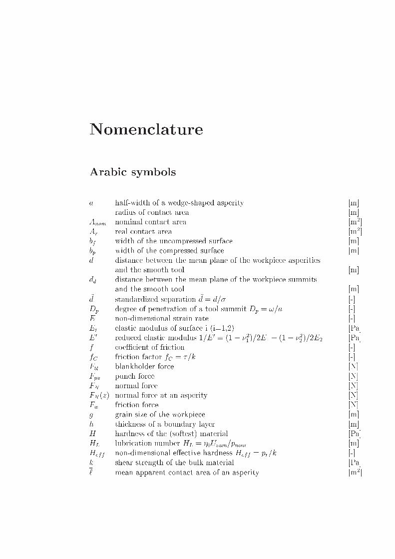
Nomenclature
Arabic symbols
a half-width of a wedge-shaped asperity [m]radius of contact area [m]
Anom nominal contact area [m2]Ar real contact area [m2]bf width of the uncompressed surface [m]bp width of the compressed surface [m]d distance between the mean plane of the workpiece asperities
and the smooth tool [m]dd distance between the mean plane of the workpiece summits
and the smooth tool [m]~d standardized separation ~d = d=� [-]Dp degree of penetration of a tool summit Dp = !=a [-]E non-dimensional strain rate [-]Ei elastic modulus of surface i (i=1,2) [Pa]E 0 reduced elastic modulus 1=E 0 = (1� �21)=2E1 + (1� �22)=2E2 [Pa]f coeÆcient of friction [-]fC friction factor fC = �=k [-]Fbl blankholder force [N]Fpu punch force [N]FN normal force [N]FN(z) normal force at an asperity [N]Fw friction force [N]g grain size of the workpiece [m]h thickness of a boundary layer [m]H hardness of the (softest) material [Pa]HL lubrication number HL = �0Usum=pnom [m]Heff non-dimensional e�ective hardness Heff = pr=k [-]k shear strength of the bulk material [Pa]
` mean apparent contact area of an asperity [m2]
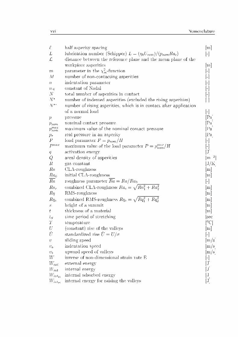
xvi Nomenclature
` half asperity spacing [m]L lubrication number (Schipper) L = (�0Usum)=(pnomRac) [-]L distance between the reference plane and the mean plane of the
workpiece asperities [m]m parameter in the �2m-function [-]M number of non-contacting asperities [-]n indentation parameter [-]nN constant of Nadai [-]N total number of asperities in contact [-]N� number of indented asperities (excluded the rising asperities) [-]N�� number of rising asperities, which is in contact after application
of a normal load [-]p pressure [Pa]pnom nominal contact pressure [Pa]pmaxnom maximum value of the nominal contact pressure [Pa]pr real pressure in an asperity [Pa]P load parameter P = pnom=H [-]Pmax maximum value of the load parameter P = pmaxnom=H [-]q activation energy [J]Q areal density of asperities [m�2]R gas constant [J/K]Ra CLA-roughness [m]Ra0 initial CLA-roughness [m]Ra roughness parameter Ra = Ra=Ra0 [-]
Rac combined CLA-roughness Rac =pRa21 +Ra22 [m]
Rq RMS-roughness [m]
Rqc combined RMS-roughness Rqc =pRq21 +Rq22 [m]
s height of a summit [m]t thickness of a material [m]tS time period of stretching [sec]T temperature [0C]U (constant) rise of the valleys [m]~U standardized rise ~U = U=� [-]v sliding speed [m/s]va indentation speed [m/s]vb upward speed of valleys [m/s]W inverse of non-dimensional strain rate E [-]Wext external energy [J]Wint internal energy [J]Wintst internal adsorbed energy [J]Wintri internal energy for raising the valleys [J]
Nomenclature xvii
z height of a workpiece asperity [m]~z standardized asperity height ~z = z=� [-]
Greek symbols
� fraction of real contact area of a single asperity [-]� fraction of real contact � = Ar=Anom [-]� radius of summits [m]�t el critical radius of tool summits above which elastic-plastic
deformation occurs [m]�t cu critical radius of tool summits below which cutting starts [m] empirical parameter in the junction growth theory of Tabor [-]Æ separation compared to the mean plane of the tool summits [m]�A area of asperity [m2]�z indentation [-]�h rise of the material in a compression test [m]` half asperity spacing [m]� nominal strain [-]�N natural strain [-]�Nst natural strain due to stretching [-]�Nbe
natural strain due to bending [-]_� strain rate [1/s]�1 energy factor [-]�2, �3 shape factor [-]�0 ambient viscosity [Pa s]� persistence parameter [-]� attack angle of a tool summit [-]�cu critical attack angle of a summit above which cutting starts [-]# angle of wedge-shaped workpiece asperity [-]� characterictic frequency of boundary layer [1/s]� characteristic frequency [1/s]�c autocorrelation length of a surface [m]�i Poisson's ratio of surface i (i = 1; 2) [-]� parameter in ideal plastic contact model [-]� areal density of summits [m�2]� standard deviation of the asperity height distribution function [m]~� standardized standard deviation ~� = �=�0 [-]�0 initial standard deviation [m]�s standard deviation of the summit height distribution function [m]
xviii Nomenclature
�y yield stress [Pa]�wh (additional) work hardening stress [Pa]& empirical parameter [-]� shear strength of boundary layer [Pa]�(z) asperity height distribution function [m�1]�s(s) summit height distribution function [m�1]~�(~z) standardized asperity height distribution function [-]� fan angle used in Sutcli�e's model [-]� parameter in work hardening contact model [-]
plasticity index = E 0=Hp�s=� [-]
! indentation of tool summit [m]
Subscripts
BL Boundary Lubricationel elasticL (normal) loadingpl plasticP ploughingS stretchingt toolw workpiecewh work hardening
Abbreviations
BL Boundary LubricationEBT Electro Beam textureEDT Electro Discharged Texture(E)HL (Elasto) Hydrodynamic LubricationMF Mill FinishedML Mixed LubricationP PloughingSFA Surface Force ApparatusSMF Sheet Metal Forming
Chapter 1
Introduction
1.1 Sheet Metal Forming (SMF) and deep draw-
ing
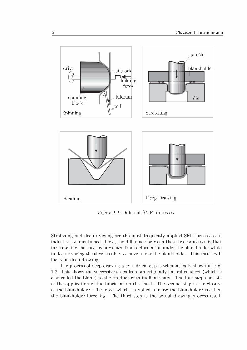
The shape of many metal products, which are used in daily life is obtained bymeans of Sheet Metal Forming (SMF) processes. SMF processes are characterizedby permanent deformation to a metal sheet. This permanent or plastic deforma-tion is attained by the application of an external load on the sheet. This loadmust be suÆciently high to ensure that after removing the load the speci�c shapeof the sheet is retained. Di�erent types of Sheet Metal Forming processes, shownin Fig. 1.1, are described brie y.
� Spinning: A circular sheet (blank) is clamped and rotated between a maledie (which possesses the shape of the �nal product) and the tailstock. Aspecial tool (a fulcrum) takes care of the deformation of the sheet.
� Stretching: In this process the sheet is �rmly clamped at its circumferenceafter which a punch deforms the sheet. The sheet receives the shape of thepunch. The deformation of the sheet is obtained from radial strain.
� Bending: Pressing the punch gradually on to the sheet, the sheet receivesthe shape of the punch. The material around the punch can move freely,so bending forces are the only forces which occur here.
� Deep drawing: In deep drawing the sheet (the blank) is put on the die, whichpossesses the shape of the product to be drawn. Then the blankholder isclosed on that part of the sheet, which is not deformed by the punch. Theblankholder prevents wrinkling of the sheet and controls the sliding of thesheet during the drawing process. After closing the blankholder, the punchis moved downwards deforming the sheet to its �nal shape.
2 Chapter 1: Introduction
spinningblock
pull
drive
holdingforce
fulcrum
punch
tailstock
die
blankholder
Spinning Stretching
Bending Deep Drawing
Figure 1.1: Di�erent SMF-processes.
Stretching and deep drawing are the most frequently applied SMF processes inindustry. As mentioned above, the di�erence between these two processes is thatin stretching the sheet is prevented from deformation under the blankholder whilein deep drawing the sheet is able to move under the blankholder. This thesis willfocus on deep drawing.
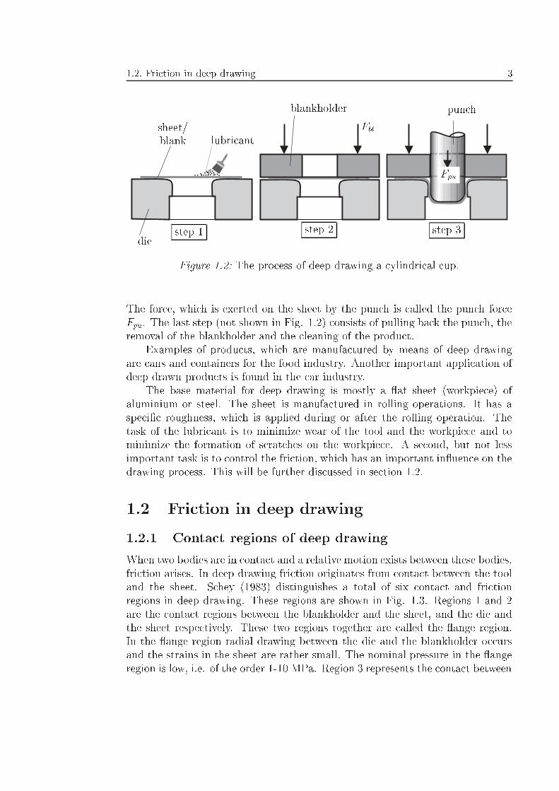
The process of deep drawing a cylindrical cup is schematically shown in Fig.1.2. This shows the successive steps from an originally at rolled sheet (which isalso called the blank) to the product with its �nal shape. The �rst step consistsof the application of the lubricant on the sheet. The second step is the closureof the blankholder. The force, which is applied to close the blankholder is calledthe blankholder force Fbl. The third step is the actual drawing process itself.
1.2. Friction in deep drawing 3
. .... .. .. .... .. .. .. .....
step 1 step 2 step 3
sheet/blank
die
blankholder punch
Fbl
Fpu
lubricant
Figure 1.2: The process of deep drawing a cylindrical cup.
The force, which is exerted on the sheet by the punch is called the punch forceFpu. The last step (not shown in Fig. 1.2) consists of pulling back the punch, theremoval of the blankholder and the cleaning of the product.
Examples of products, which are manufactured by means of deep drawingare cans and containers for the food industry. Another important application ofdeep drawn products is found in the car industry.
The base material for deep drawing is mostly a at sheet (workpiece) ofaluminium or steel. The sheet is manufactured in rolling operations. It has aspeci�c roughness, which is applied during or after the rolling operation. Thetask of the lubricant is to minimize wear of the tool and the workpiece and tominimize the formation of scratches on the workpiece. A second, but not lessimportant task is to control the friction, which has an important in uence on thedrawing process. This will be further discussed in section 1.2.
1.2 Friction in deep drawing
1.2.1 Contact regions of deep drawing
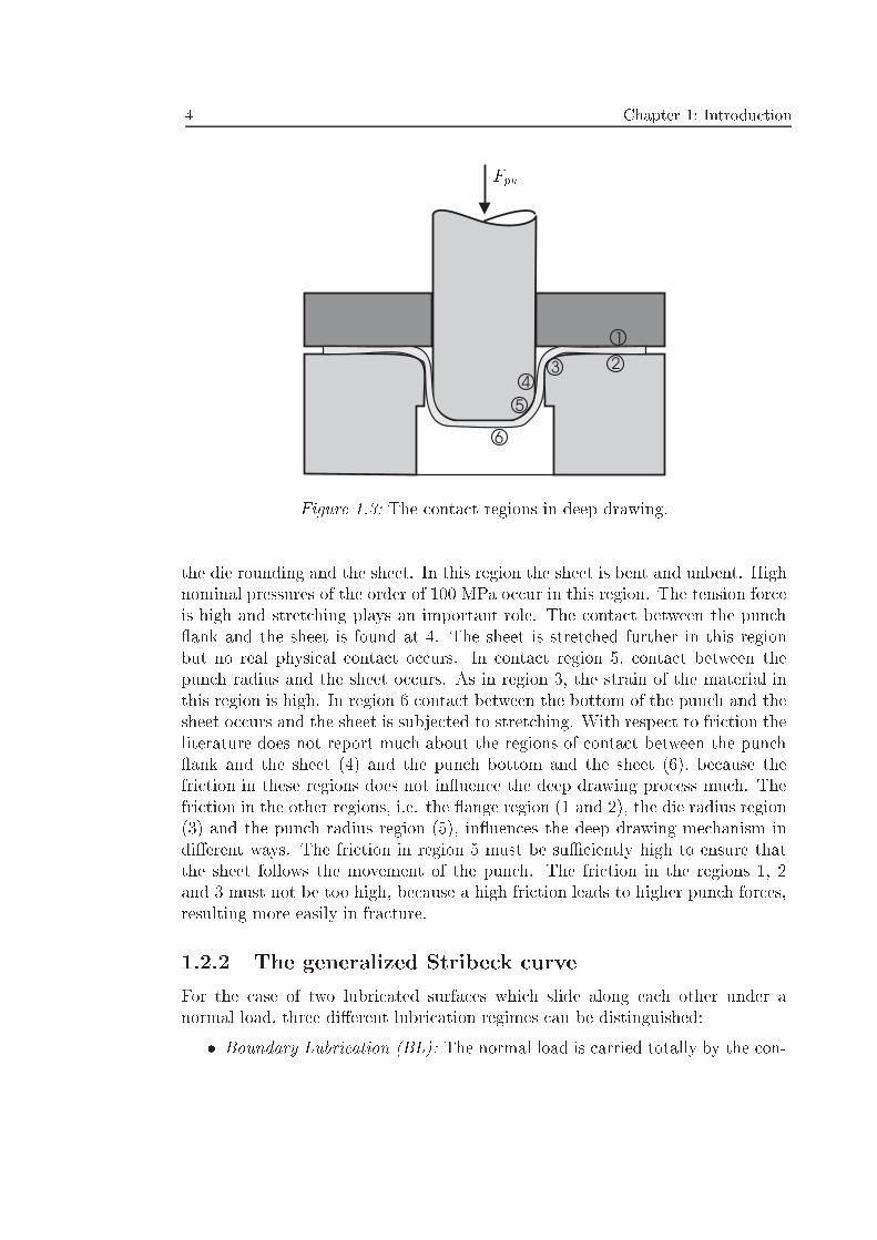
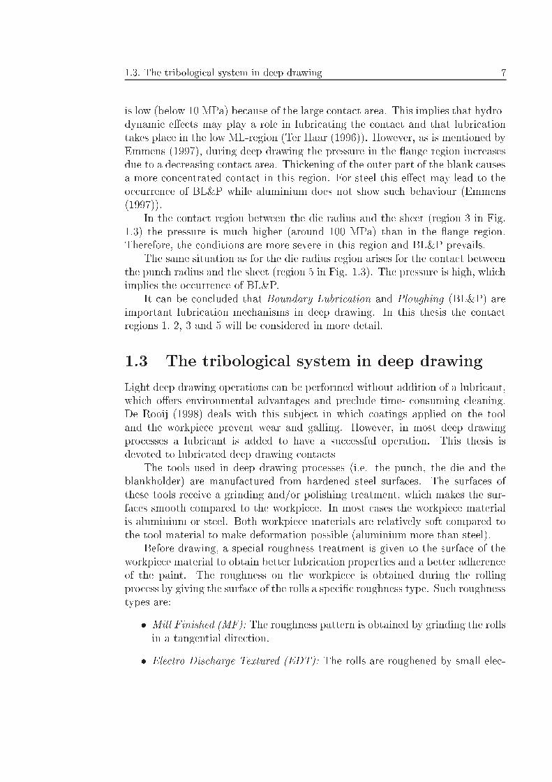
When two bodies are in contact and a relative motion exists between these bodies,friction arises. In deep drawing friction originates from contact between the tooland the sheet. Schey (1983) distinguishes a total of six contact and frictionregions in deep drawing. These regions are shown in Fig. 1.3. Regions 1 and 2are the contact regions between the blankholder and the sheet, and the die andthe sheet respectively. These two regions together are called the ange region.In the ange region radial drawing between the die and the blankholder occursand the strains in the sheet are rather small. The nominal pressure in the angeregion is low, i.e. of the order 1-10 MPa. Region 3 represents the contact between
4 Chapter 1: Introduction
6
5
43 2
1
Fpu
Figure 1.3: The contact regions in deep drawing.
the die rounding and the sheet. In this region the sheet is bent and unbent. Highnominal pressures of the order of 100 MPa occur in this region. The tension forceis high and stretching plays an important role. The contact between the punch ank and the sheet is found at 4. The sheet is stretched further in this regionbut no real physical contact occurs. In contact region 5, contact between thepunch radius and the sheet occurs. As in region 3, the strain of the material inthis region is high. In region 6 contact between the bottom of the punch and thesheet occurs and the sheet is subjected to stretching. With respect to friction theliterature does not report much about the regions of contact between the punch ank and the sheet (4) and the punch bottom and the sheet (6), because thefriction in these regions does not in uence the deep drawing process much. Thefriction in the other regions, i.e. the ange region (1 and 2), the die radius region(3) and the punch radius region (5), in uences the deep drawing mechanism indi�erent ways. The friction in region 5 must be suÆciently high to ensure thatthe sheet follows the movement of the punch. The friction in the regions 1, 2and 3 must not be too high, because a high friction leads to higher punch forces,resulting more easily in fracture.
1.2.2 The generalized Stribeck curve
For the case of two lubricated surfaces which slide along each other under anormal load, three di�erent lubrication regimes can be distinguished:
� Boundary Lubrication (BL): The normal load is carried totally by the con-
1.2. Friction in deep drawing 5
tacting asperities, which exist on both surfaces. These surfaces are pro-tected from dry contact by thin boundary layers, which are attached to thesurfaces.
� Mixed Lubrication (ML): A part of the load is carried by contacting asper-ities (separated by boundary layers) and another part of the load is carriedby the lubricant �lm.
� (Elasto) Hydrodynamic Lubrication ((E)HL): The load is carried totallyby the full �lm and contact between the opposing surfaces does not occur.When the normal load is high, elastic deformation of the surfaces may occur.In this case the term Elasto Hydrodynamic Lubrication is used to de�nethe lubrication mechanism.
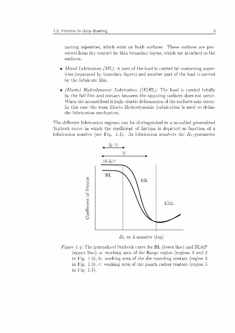
The di�erent lubrication regimes can be distinguished in a so-called generalizedStribeck curve in which the coeÆcient of friction is depicted as function of alubrication number (see Fig. 1.4). As lubrication numbers the HL-parameter
HL or L-number (log)
CoeÆcientoffriction
BLML
EHL
a
b c
BL&P
Figure 1.4: The generalized Stribeck curve for BL (lower line) and BL&P(upper line); a: working area of the ange region (regions 1 and 2in Fig. 1.3), b: working area of the die rounding contact (region 3in Fig. 1.3), c: working area of the punch radius contact (region 5in Fig. 1.3).
6 Chapter 1: Introduction
and the L-number are used. HL is de�ned as (Schipper (1988)):
HL =�0Usumpnom
(1.1)
with �0 as the (ambient) viscosity of the lubricant, Usum as the sum velocity of thesurfaces and pnom as the mean nominal pressure. The dimensionless L-number isde�ned as:
L = HL=Rac (1.2)
in which Rac is the combined CLA-roughness of both surfaces. Another numberwhich determines the lubrication regime is the �-value, de�ned as h=Rqc withh as the mean �lm thickness and Rqc as the combined RMS-roughness (Bair &Winer (1982)). Low values of HL, L or � imply the occurrence of Boundary Lu-brication, while for high values of HL, L or � Hydrodynamic Lubrication occurs.For intermediate values of HL, L and �, the contact is lubricated in the MixedLubrication regime. For more detailed information concerning the lubricationnumbers the reader is referred to Schipper (1988).
1.2.3 Boundary Lubrication and Ploughing
During BL, friction is entirely due to shear between the boundary layers, attachedto the surfaces. The existence of BL was �rst proven by Hardy & Doubleday(1922). The way in which sliding in the BL-regime takes place is very complicatedand described only for simple cases, i.e. when the chemical structure of thelayers is known. A \global" view concerning the sliding mechanism is given, forexample, by Briscoe, Scruton & Willis (1973) and Tabor (1982). In chapter 2more attention is paid to BL.
The idea that in realistic situations, friction is only due to shear between theboundary layers, was at �rst rejected by Bowden & Tabor (1954). For roughsurfaces and/or a large di�erence in hardness of the two sliding surfaces, frictioncan also be caused by plastic deformation of asperities. In this thesis this sourceof friction is called Ploughing. Because in deep drawing contact occurs betweensurfaces with a relatively large di�erence in hardness, ploughing also contributesto friction. The abbreviation BL&P is introduced to de�ne the combined actionof BL and ploughing (P). Possible exceptions are considered in the text.
1.2.4 Lubrication mechanisms in deep drawing
The three di�erent contact regions mentioned in section 1.2.1, which are impor-tant in deep drawing processes, i.e. regions 1,2,3 and 5 of Fig. 1.3, operate indi�erent lubrication regimes (see also Fig. 1.4). In the ange region, the pressure
1.3. The tribological system in deep drawing 7
is low (below 10 MPa) because of the large contact area. This implies that hydro-dynamic e�ects may play a role in lubricating the contact and that lubricationtakes place in the low ML-region (Ter Haar (1996)). However, as is mentioned byEmmens (1997), during deep drawing the pressure in the ange region increasesdue to a decreasing contact area. Thickening of the outer part of the blank causesa more concentrated contact in this region. For steel this e�ect may lead to theoccurrence of BL&P while aluminium does not show such behaviour (Emmens(1997)).
In the contact region between the die radius and the sheet (region 3 in Fig.1.3) the pressure is much higher (around 100 MPa) than in the ange region.Therefore, the conditions are more severe in this region and BL&P prevails.
The same situation as for the die radius region arises for the contact betweenthe punch radius and the sheet (region 5 in Fig. 1.3). The pressure is high, whichimplies the occurrence of BL&P.
It can be concluded that Boundary Lubrication and Ploughing (BL&P) areimportant lubrication mechanisms in deep drawing. In this thesis the contactregions 1, 2, 3 and 5 will be considered in more detail.
1.3 The tribological system in deep drawing
Light deep drawing operations can be performed without addition of a lubricant,which o�ers environmental advantages and preclude time- consuming cleaning.De Rooij (1998) deals with this subject in which coatings applied on the tooland the workpiece prevent wear and galling. However, in most deep drawingprocesses a lubricant is added to have a successful operation. This thesis isdevoted to lubricated deep drawing contacts
The tools used in deep drawing processes (i.e. the punch, the die and theblankholder) are manufactured from hardened steel surfaces. The surfaces ofthese tools receive a grinding and/or polishing treatment, which makes the sur-faces smooth compared to the workpiece. In most cases the workpiece materialis aluminium or steel. Both workpiece materials are relatively soft compared tothe tool material to make deformation possible (aluminium more than steel).
Before drawing, a special roughness treatment is given to the surface of theworkpiece material to obtain better lubrication properties and a better adherenceof the paint. The roughness on the workpiece is obtained during the rollingprocess by giving the surface of the rolls a speci�c roughness type. Such roughnesstypes are:
� Mill Finished (MF): The roughness pattern is obtained by grinding the rollsin a tangential direction.
� Electro Discharge Textured (EDT): The rolls are roughened by small elec-
8 Chapter 1: Introduction
tric discharges. In this way, when the sheet is rolled, craters arise on theworkpiece surface. EDT has a random nature.
� Electron Beam Textured (EBT): An electron beam is used to manufacturecraters in the surface of the roll. This is performed in such a way that adeterministic distribution of the roughness is obtained.
Not only the type of roughness but also the magnitude of the roughness may bedi�erent for di�erent roughness types. For example, MF surfaces mostly possessa lower roughness than EDT and EBT surfaces.
In deep drawing processes a mineral oil oftenly serves as a lubricant. In mostcases additives are added to the mineral oil, the base oil, to obtain special prop-erties of the lubricant. The function of these additives can vary from preventingharmful chemical changes of the oil or the surfaces to improving the e�ectivenessof lubrication as lowering the friction and/or wear. Besides all these functions,additives are sometimes used for special applications of the system. A review ofthe role of some additives and their interaction is given by Spikes (1989).
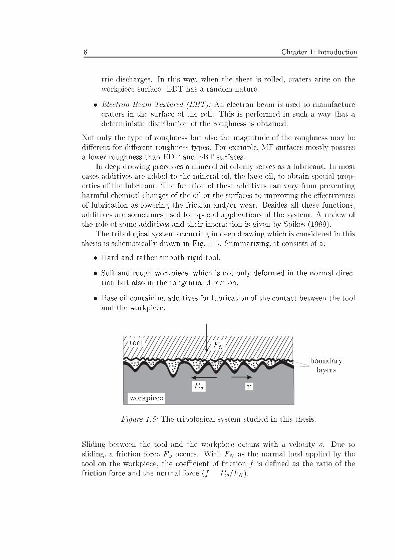
The tribological system occurring in deep drawing which is considered in thisthesis is schematically drawn in Fig. 1.5. Summarizing, it consists of a:
� Hard and rather smooth rigid tool.
� Soft and rough workpiece, which is not only deformed in the normal direc-tion but also in the tangential direction.
� Base oil containing additives for lubrication of the contact between the tooland the workpiece.
workpiece
tool
boundarylayers
FN
Fw v
Figure 1.5: The tribological system studied in this thesis.
Sliding between the tool and the workpiece occurs with a velocity v. Due tosliding, a friction force Fw occurs. With FN as the normal load applied by thetool on the workpiece, the coeÆcient of friction f is de�ned as the ratio of thefriction force and the normal force (f = Fw=FN).
1.4. The objective of this research 9
1.4 The objective of this research
It was shown earlier that BL&P play an important role in the lubrication of deepdrawing processes. Therefore, it is necessary to obtain a better understanding ofthe working of BL&P. Regarding BL&P, most attention in the literature is paidto experimental work. In this thesis a model will be developed, which can beused to calculate the coeÆcient of friction occurring in the BL&P-regime. Thismodel is an important tool to predict the friction in the BL&P-regime for deepdrawing processes. Compared with experimental work, the model o�ers a quickerand cheaper method for calculating the coeÆcient of friction. In this thesis noattention is paid to dry contact between surfaces. Wear is also not taken intoaccount.
1.5 Overview
A review of the literature available will be presented in chapter 2. BoundaryLubrication and Ploughing (BL&P) will be explained more extensively in thischapter. Chapter 3 will be devoted to the development of a new contact model,which can be applied to describe a deep drawing contact. This contact modelis necessary for the development of the friction model. In chapter 4 the con-tact model is extensively tested by means of several experiments. Chapter 5 isdedicated to the description of the friction model including BL and ploughing.In chapter 6 the theoretical results of the friction model will be compared withexperimental results. Conclusions and recommendations will be given in chapter7.

10 Chapter 1: Introduction
Chapter 2
Boundary Lubrication andPloughing (BL&P) - literature
2.1 Introduction
In the previous chapter a distinction is made between Boundary Lubrication (BL)and Ploughing (P). In this chapter these two sliding mechanisms are studied inmore detail on the basis of a review of the literature.
Section 2.2 focusses on the treatment of boundary lubrication (BL). Becauseof the complicated relation between friction in the BL regime on the one handand the chemical and physical properties of the lubricant and the surface and theoperational parameters on the other hand, most studies considering BL consistof experimental work. Section 2.3 deals with the ploughing mechanism. Somesimple relations will be given for the coeÆcient of friction of hard ploughingasperities with di�erent geometries. In section 2.4 a model for describing BL&Pis brie y discussed. The chapter ends with a short summary.
2.2 Boundary Lubrication (BL)
In Hardy & Doubleday (1922) it was postulated that for sliding metallic surfaces,covered by a thin monolayer of hydrocarbon, alcohol or fatty acids, a frictionmechanism occurred, which di�ers from the well known hydrodynamic lubricationmechanism. It was discovered that metallic surfaces were totally protected by aboundary �lm which was adsorbed to the surfaces. During sliding the friction isdue to shear of these boundary layers. The reducing e�ect of boundary layers onthe coeÆcient of friction is further con�rmed in an enormous number of papers.Some examples of the working of boundary layers are given in Langmuir (1920),Bowden & Leben (1940), Bowden & Tabor (1954) and Jahanmir & Beltzer (1986).
12 Chapter 2: Boundary Lubrication and Ploughing (BL&P) - literature
2.2.1 Formation of boundary layers
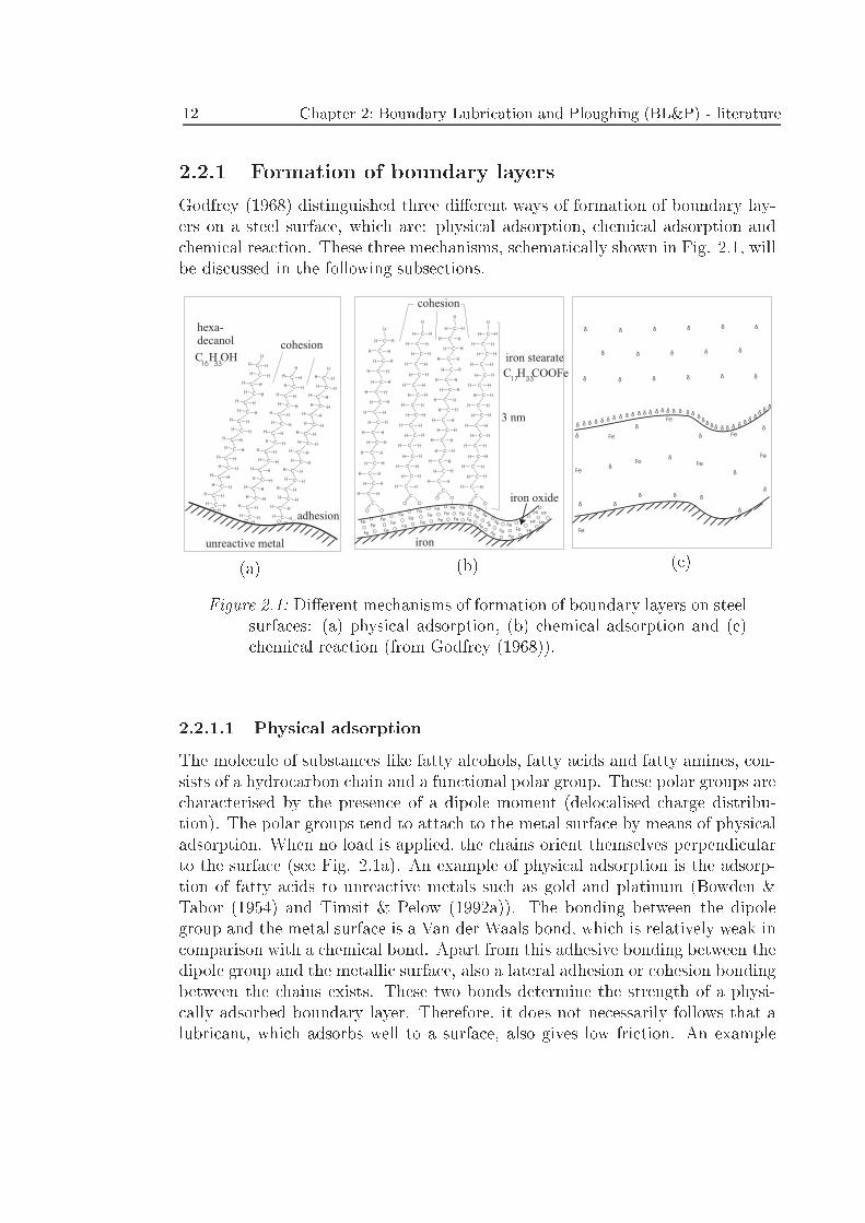
Godfrey (1968) distinguished three di�erent ways of formation of boundary lay-ers on a steel surface, which are: physical adsorption, chemical adsorption andchemical reaction. These three mechanisms, schematically shown in Fig. 2.1, willbe discussed in the following subsections.
HH C
C H
H
O H
H
C H
HH
H
C
C H
HH
H
C
C H
HH
H
C
C H
HH
H
C
C H
HH
H
C
C H
HH
H
C
C H
HH
H
C
HH C
C H
H
O H
H
C H
HH
H
C
C H
HH
H
C
C H
HH
H
C
C H
HH
H
C
C H
HH
H
C
C H
HH
H
C
C H
HH
H
C
C H
H
O H
H
C H
HH
H
C
C H
HH
H
C
C H
HH
H
C
C H
HH
H
C
C H
HH
H
C
C H
HH
H
C
C H
HH
H
C
HH C
FeFe
Fe
Fe
Fe
Fe Fe
Fe
Fe
Fe
Fe
FeFe
O Fe
Fe
OFe
Fe
OFe
Fe
OFe
FeO
Fe
FeO
Fe
FeO
Fe
Fe
OFe
Fe
O
OFe
O
OFe
O
O
Fe
O
O
FeO
O
FeO
O
Fe
O
O FeO
OFe
O
O
OO
FeFe
Fe
Fe
Fe
Fe
OO
OO
OO Fe
O
O
C
OO
H HC
H HC
H HC
H HC
H HC
H HC
H C
H C
H HC
H HC
H
H
H HC
H HC
H
H HC
H HC
H HC
H HC
C
OO
H HC
H HC
H HC
H HC
H HC
H HC
H C
H C
H HC
H HC
H
H
H HC
H HC
H
H HC
H HC
H HC
H HC
C
OO
H HC
H HC
H HC
H HC
H HC
H HC
H C
H C
H HC
H HC
H
H
H HC
H HC
H
H HC
H HC
H HC
H HC
C
OO
H HC
H HC
H HC
H HC
H HC
H HC
H C
H C
H HC
H HC
H
H
H HC
H HC
H
H HC
H HC
H HC
H HC
δδ δ
δ
δ
δ
δ
δ
δ
δ
δ
δ
δ
δ
δ
δ
δ
δ δ
δ
δ δ
δ δ δδ δ δδ
δ δ δ δ δ δδ
δ δ δδ
δδ δ δ δ
δ δ δδ
δδ δ δ
δ
δδδ
δδ
δ
δδ
δ
δδ
δ
unreactive metal
adhesion
iron
3 nm
iron oxide
iron stearatecohesion
cohesion
C H OH
C H COOFe
hexa-decanol
16
17
33
33
(a) (b) (c)
Figure 2.1: Di�erent mechanisms of formation of boundary layers on steelsurfaces: (a) physical adsorption, (b) chemical adsorption and (c)chemical reaction (from Godfrey (1968)).
2.2.1.1 Physical adsorption
The molecule of substances like fatty alcohols, fatty acids and fatty amines, con-sists of a hydrocarbon chain and a functional polar group. These polar groups arecharacterised by the presence of a dipole moment (delocalised charge distribu-tion). The polar groups tend to attach to the metal surface by means of physicaladsorption. When no load is applied, the chains orient themselves perpendicularto the surface (see Fig. 2.1a). An example of physical adsorption is the adsorp-tion of fatty acids to unreactive metals such as gold and platinum (Bowden &Tabor (1954) and Timsit & Pelow (1992a)). The bonding between the dipolegroup and the metal surface is a Van der Waals bond, which is relatively weak incomparison with a chemical bond. Apart from this adhesive bonding between thedipole group and the metallic surface, also a lateral adhesion or cohesion bondingbetween the chains exists. These two bonds determine the strength of a physi-cally adsorbed boundary layer. Therefore, it does not necessarily follows that alubricant, which adsorbs well to a surface, also gives low friction. An example
2.2. Boundary Lubrication (BL) 13
is given by Bowden & Tabor (1954) who showed that paraÆn oil which doesnot possess a polar group, gives the same friction as alcohol, although alcoholpossesses a polar group and adsorbs much better to a metal surface.
2.2.1.2 Chemical adsorption
Chemical adsorption or chemisorption is characterized by two stages. First, phys-ical adsorption of the dipole group at the end of a molecular chain to the surfaceoccurs. After physical adsorption, a chemical reaction occurs between the surfaceand the polar group. The chemical reaction depends on the chemical reactivity ofthe surface and environmental circumstances. An example of the in uence of theenvironment is given by Akhmatov (1966). In a humid environment, adsorbedstearic acid reacts with metal powders (chemical adsorption takes place) whilea dry environment inhibits the occurrence of a chemical reaction. However, ina review, Campbell (1969) describes exceptions to these �ndings. For example,oleic acid is e�ective for cutting aluminium and steel under both dry and wetconditions. Possibly, the environmental conditions in the dry case situation weredi�erent in the two tests. It is also known that a thick oxide layer enables a betterchemical adsorption and produces less friction (for example, Komvopoulos, Saka& Suh (1986)). To conclude, a general rule which determines whether physicalor chemical adsorption occurs, does not exist.
As is shown in Fig. 2.1b, stearic acid (C17H35COOH) forms a soap, i.e.iron stearate (C17H35COOFe), on an iron oxide layer. Fatty acids on aluminiumoxide also leads to chemical adsorption (Timsit & Pelow (1992b)). Therefore,for deep drawing aluminium and steel sheets, it is believed that fatty acids(CnH2n+1COOH) form metallic soaps (CnH2n+1COOM) on metals. M standsfor a metal ion while n is the number of carbon atoms in the hydrocarbon chain.
2.2.1.3 Chemical reaction
Some combinations of uids and substrates do not lead to physical adsorptionof these substances to the surface. In some cases a (direct) chemical reactionbetween the surface and the boundary lubricant occurs. A reaction product isformed (see Fig. 2.1c) which serves as an excellent medium for transmittingfriction forces. For example, in this way so-called extreme pressure lubricants(EP-lubricants) work, which possess friction reducing qualities. Cheng, Ling &Winer (1973) and Sakurai (1981) summarize the role chemical reactions play inBL for di�erent lubricants and surface materials. The science which is concernedwith this phenomenon is called tribochemistry or mechano-chemistry. No furtherattention is paid to this subject here.
14 Chapter 2: Boundary Lubrication and Ploughing (BL&P) - literature
2.2.2 Friction of boundary layers
In spite of an overwhelming interest in the literature, BL is still poorly un-derstood. Regarding the molecular mechanism of friction of chemically reactedboundary layers, no theory has yet been proposed in the literature. In this sec-tion the friction of physically and chemically adsorbed boundary layers is furtherdiscussed.
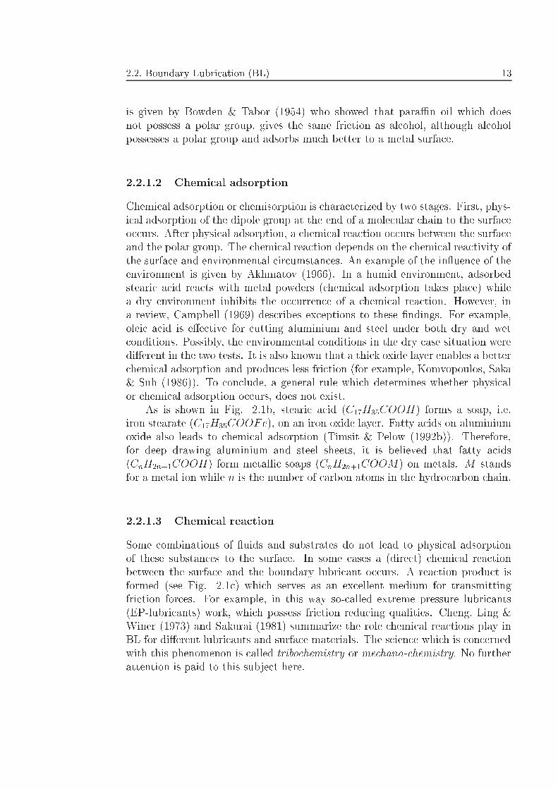
The friction force Fw is due to shear in the plane between the two bound-ary layers, shown schematically in Fig. 2.2, with FN as the normal load and
FN
v
COOH-group
CH3-group
plane of shear
Fw
Figure 2.2: Sliding of boundary layers of acids along each other in a cir-cular contact with mean pressure p and speed v.
v as the sliding speed. Sutcli�e, Taylor & Cameron (1978) distinguished twocauses of friction. The �rst cause of friction is when attractive forces betweenopposing layers are overcome (including losses due to internal rotation barriers).The second cause of friction is the lifting of tail groups of one layer over thetail groups of the other layer during sliding. This model was later called thecobblestone theory (Tabor (1982) and Homola, Israelachvili, McGuiggan & Gee(1990)). Despite theoretical work on the sliding and friction of adsorbed layers,such as the cobblestone theory or more sophisticated molecular dynamics studies(Landman, Luedtke & Ringer (1992), Glosli & McClelland (1993) and Dowson(1994)), values for the coeÆcient of friction are mainly obtained by performingmeasurements. In subsequent sections some results of these measurements willbe discussed in more detail.
2.2.2.1 Experimental details
Most experiments which will be discussed in this section, have been performed ona so-called Surface Force Apparatus (SFA). In an SFA the friction is measured ina circular contact between a sphere and a plane or between two crossed cylinders.
2.2. Boundary Lubrication (BL) 15
The sphere or one of the cylinders makes a reciprocating movement. To preventdry contact (adhesion) and ploughing e�ects, the lubricated surfaces are made ofmica or glass, which possess a very low roughness (the CLA-roughness is in theorder of a few nanometers). Because of the low roughness and the high hardnessof the mica and glass surfaces, the surfaces deform elastically. By using glass ormica surfaces, possible break-down (i.e. dry contact between the surfaces) canbe observed during sliding. For most of the systems discussed here, no break-down of the �lm was detected, which implies that friction was only due to shearbetween the boundary layers. One or more boundary layers are deposited onthe surfaces according to special techniques as Langmuir-Blodgett (LB) deposi-tion (Blodgett (1935)) and retraction from the melt (Bigelow, Pickett & Zisman(1946)). Experimental results, published in the literature, generally report valuesof the shear strength � , which are obtained by dividing the friction force Fw bythe Hertz contact area A, which carries the normal load.
2.2.2.2 In uence of the pressure
Several publications have appeared, in which the shear strength � is measuredas a function of the mean Hertzian contact pressure p. Here, a number of resultsobtained from the literature are �tted and the �ts are shown in Fig. 2.3a. Therelation between the coeÆcient of friction (f = �=p) and the pressure p is plottedin Fig. 2.3b. The numbers in Fig. 2.3 correspond with the numbers mentionedin the following list:
1. Briscoe et al. (1973) measured the shear strength of one, three and �veLB monolayers of calcium stearate (C17H35COOCa) adsorbed on glass at atemperature T of 20 0C and a sliding speed v of 0.06 mm/s. The di�erencesdue to the di�erent number of layers fell within the experimental error.
2. Briscoe et al. (1973) also report shear strength measurements with mono-layers of stearic acid (C17H35COOH) retracted from the melt for T = 20 0Cand v = 0.06 mm/s.
3. Similar experiments for LB monolayers of stearic acid on mica were carriedout by Briscoe & Evans (1982) for T = 21 0C and v = 3:6 �m/s.
4. Investigating the in uence of another surface material on the friction, Tim-sit & Pelow (1992b) measured the shear strength of LB monolayers of stearicacid on a glass slider and an aluminium coated glass substrate for T = 20 0Cand v=0.06 mm/s.
5. A uid with a di�erent structure than stearic acid and stearates, i.e. cal-cium carbonate (CaCO3) in dodecane, was tested by Georges & Mazuyer
16 Chapter 2: Boundary Lubrication and Ploughing (BL&P) - literature
(1991) on three di�erent apparatuses, using di�erent substrate materialsand di�erent operational parameters.
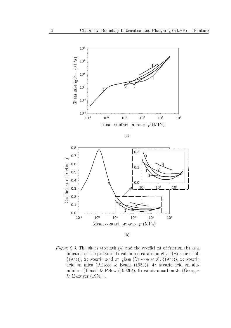
The experiments cover a wide pressure range, varying from 0.13 MPa to 3 GPa.From p = 1 MPa to p � 300 MPa Fig. 2.3a shows that the increase of the shearstrength is less than the increase of the pressure p, which results in a decreasingcoeÆcient of friction with increasing pressure. For pressures larger than 300 MPathe coeÆcient of friction increases when the pressure is increased. For LB layersof stearic acid adsorbed to aluminium (4), a larger shear strength is found thanfor the system stearic acid - glass (2), which is probably due to local disruptionof the layers, resulting in adhesive forces between aluminium and glass.
The following explanation is given for the results of shearing acid and stearateboundary layers shown in Fig. 2.3. The sliding process of these layers involvesthe shear of molecular chains along each other. The layers are physically or chem-ically adsorbed to the surface. A decreasing coeÆcient of friction for increasingpressures, is attributed to an increasing degree of orientation of the chains inthe sliding direction. Schematically this orientation is shown in Fig. 2.2. Theincrease of the friction force for increasing normal pressures above 300 MPa isdue to squeezing the molecular chains together. The two e�ects have an oppositee�ect on the coeÆcient of friction. Whether an increase or a decrease of thecoeÆcient of friction occurs depends on which of the e�ects is stronger.
The mean Hertzian pressure p in Fig. 2.3 is equivalent to the pressure proccurring in an asperity of the workpiece in contact with a smooth tool. Forpure plasticallly deforming asperities (i.e., elastic deformations are neglected), prequals the hardness H of the workpiece. In deep drawing aluminium and steelblanks, H varies from 250 MPa for soft aluminium to about 2 GPa for steel.Therefore, in deep drawing, this pressure region is of most practical interest.
2.2.2.3 In uence of the temperature
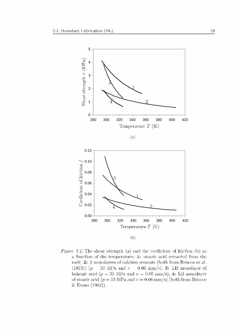
In Fig. 2.4a the shear strength is plotted versus the temperature for stearicand behenic acid and calcium stearate adsorbed to glass. The �ts are obtainedfrom experimental work by Briscoe et al. (1973) and Briscoe & Evans (1982).Fig. 2.4b shows the corresponding values of the coeÆcients of friction. Althoughexceptions exist (not shown in Fig. 2.4), in general it can be stated that whenthe temperature of a boundary layer is increased, the shear strength and thecoeÆcient of friction decrease.
2.2.2.4 In uence of the speed
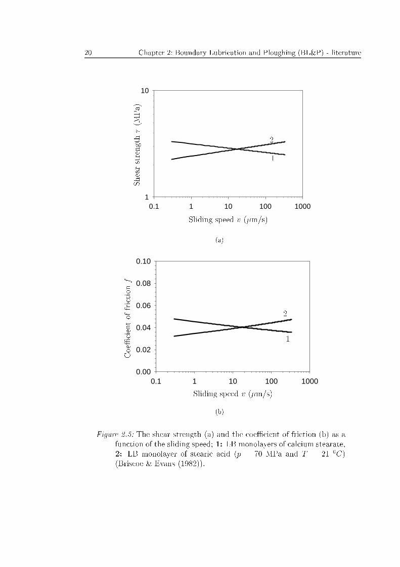
A few studies report on the in uence of the sliding speed v on the shear strength.In these studies, the speed is low, which makes temperature e�ects negligible.Briscoe & Tabor (1978) and Briscoe & Evans (1982) studied the in uence of
2.2. Boundary Lubrication (BL) 17
the speed and found di�erent results for di�erent uids. Fig. 2.5 shows theresults for LB monolayers of stearic acid and calcium stearate adsorbed on micasurfaces. Stearic acid shows an increasing shear strength with increasing speedwhile calcium stearate shows the opposite e�ect. According to Briscoe & Tabor(1978) two physical phenomena are responsible for the dependence of � on v. The�rst e�ect concerns the in uence of the speed on the strain rate in the boundary�lm, which leads to an increase of � . The strain rate is de�ned as v=h in whichh is the thickness of the boundary layer. The second e�ect of the speed hasto do with the visco-elastic behaviour of the boundary layers. This means thatwhen a normal load is applied, the monolayers need some time to respond tothe applied normal load. In other words, the \real load", which is carried bythe monolayers, is smaller than the applied load. The time of contact betweentwo monolayers is an important parameter, which determines the importance ofvisco-elastic behaviour. The measured coeÆcient of friction is smaller when thevisco-elastic e�ect is larger. The larger the contact time t (t = v=d with d asthe Hertzian diameter of the contact area), the more time the molecules get torespond to the application of the normal load, resulting in a smaller visco-elastice�ect.
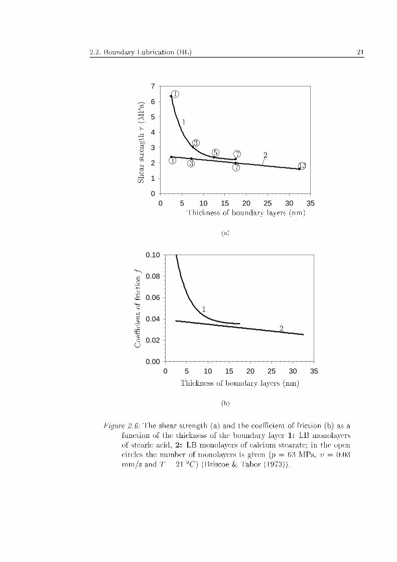
2.2.2.5 In uence of the thickness of LB monolayers
Briscoe & Tabor (1973) were able to accurately measure the in uence of thenumber of monolayers on the shear strength. Stearic acid and calcium stearateLB monolayers were deposited on glass. The thickness of one monolayer amountsto about 2.5 nm. Fig. 2.6 shows the results for p = 63 MPa, v = 0.03 mm/s andT = 21 0C. It can be concluded that increasing the number of monolayers resultsin a decrease of the shear strength. This e�ect is larger for stearic acid than forcalcium stearate.
2.2.2.6 Combined in uence of parameters - curve �ts
For later use in this thesis, a general relation for � as a function of the pressure p,the temperature T and the sliding speed v is needed. Based on the results shownin Fig. 2.3a, the following relation between � and p is proposed:
� = Cpn (2.1)
with C and n constants (n > 0). C and n can have di�erent values when theslope in the log � � log p graph is di�erent.
Based on results shown in Fig. 2.4a and following the analysis of Briscoeet al. (1973), the Eyring relation is assumed to describe the relation between �and T :
� = �0eq=RT (2.2)
18 Chapter 2: Boundary Lubrication and Ploughing (BL&P) - literature
10-1 100 101 102 103 104
10-2
10-1
100
101
102
103
Mean contact pressure p (MPa)
Shearstrength�( MPa)
1
2 3
4
5
(a)
10-1 100 101 102 103 1040.0
0.1
0.2
0.3
0.4
0.5
0.6
0.7
0.8
101 102 103
0.0
0.1
0.2
Mean contact pressure p (MPa)
CoeÆcientoffrictionf
1
1
2
2
3
3
4
4
5
5
(b)
Figure 2.3: The shear strength (a) and the coeÆcient of friction (b) as afunction of the pressure 1: calcium stearate on glass (Briscoe et al.(1973)), 2: stearic acid on glass (Briscoe et al. (1973)), 3: stearicacid on mica (Briscoe & Evans (1982)), 4: stearic acid on alu-minium (Timsit & Pelow (1992b)), 5: calcium carbonate (Georges& Mazuyer (1991)).
2.2. Boundary Lubrication (BL) 19
280 300 320 340 360 380 400 4200
1
2
3
4
5
Temperature T (K)
Shearstrength�(MPa )
1
2
3
4
(a)
280 300 320 340 360 380 400 4200.00
0.02
0.04
0.06
0.08
0.10
0.12
Temperature T (K)
CoeÆcientoffrictio nf
1
2
3
4
(b)
Figure 2.4: The shear strength (a) and the coeÆcient of friction (b) asa function of the temperature; 1: stearic acid retracted from themelt, 2: 3 monolayers of calcium stearate (both from Briscoe et al.(1973)) (p = 50 MPa and v = 0.06 mm/s), 3: LB monolayer ofbehenic acid (p = 35 MPa and v = 0.06 mm/s), 4: LB monolayerof stearic acid (p = 53 MPa and v = 0.06 mm/s) (both from Briscoe& Evans (1982)).
20 Chapter 2: Boundary Lubrication and Ploughing (BL&P) - literature
0.1 1 10 100 10001
10
Sliding speed v (�m/s)
Shearstrength�(MPa)
1
2
(a)
0.1 1 10 100 10000.00
0.02
0.04
0.06
0.08
0.10
Sliding speed v (�m/s)
CoeÆcientoffrictionf
1
2
(b)
Figure 2.5: The shear strength (a) and the coeÆcient of friction (b) as afunction of the sliding speed; 1: LB monolayers of calcium stearate,2: LB monolayer of stearic acid (p = 70 MPa and T = 21 0C)(Briscoe & Evans (1982)).
2.2. Boundary Lubrication (BL) 21
0 5 10 15 20 25 30 350
1
2
3
4
5
6
7
Thickness of boundary layers (nm)
Shearstrength�(MPa)
1
23
35
7
71
1
13
(a)
0 5 10 15 20 25 30 350.00
0.02
0.04
0.06
0.08
0.10
Thickness of boundary layers (nm)
CoeÆcientoffrictio nf
1
2
(b)
Figure 2.6: The shear strength (a) and the coeÆcient of friction (b) as afunction of the thickness of the boundary layer 1: LB monolayersof stearic acid, 2: LB monolayers of calcium stearate; in the opencircles the number of monolayers is given (p = 63 MPa, v = 0.03mm/s and T = 21 0C) (Briscoe & Tabor (1973)).
22 Chapter 2: Boundary Lubrication and Ploughing (BL&P) - literature
In eq. (2.2) �0 is a constant, R is the gas constant and q is the so-called activationenergy. q is a measure for the mobility of molecules. The higher the value of q,the larger the mobility of the molecules.
On the basis of the results shown in Fig. 2.5a, it is assumed that � is afunction of v according to:
� = Dvm (2.3)
with D and m constants. When � increases with increasing v, m > 0; in the casethat � decreases with increasing v, m < 0.
Taking the natural logarithm of eq. (2.1) and eq. (2.2) gives, respectively:
ln � = lnC + n ln p (2.4)
and:
ln � = ln �0 +q
RT(2.5)
If it is assumed that n is independent of T , eq. (2.4) and eq. (2.5) can becombined to:
ln � = F +q
RT+ n ln p (2.6)
in which F is another constant. Further, it is assumed that the strain rate e�ectof v, described in section 2.2.2.4, in uences F . Then F can be expressed asfollows:
F = � 00 ln
�v
h
1
�
�(2.7)
in which � 00 is a constant and � is de�ned as a \characteristic" frequency (Briscoe& Tabor (1978)). Finally, it is assumed that the visco-elastic e�ect of the speedonly in uences n. Then, n can be expressed as:
n = n0 exp
��vd
1
�
�(2.8)
in which n0 is a constant and � is another \characteristic" frequency. Eq. (2.8)implies that for high speeds n! 0, implying that the boundary layers do not gettime to respond to the application of the normal load for high speeds. Decreasingv results in a larger in uence on ln � . The limit is attained when v ! 0 forwhich n ! n0. In this case the layers has the maximum time to respond to theapplication of the normal load. So, 0 < n < n0. This is in agreement with the
2.2. Boundary Lubrication (BL) 23
conclusions drawn in section 2.2.2.4.Substituting eq. (2.7) and eq. (2.8) in eq. (2.6) gives:
ln � = � 00 ln
�v
h
1
�
�+
q
RT+ n0 exp
��vd
1
�
�ln p (2.9)
Eq. (2.9) is a general empirical-theoretical expression for � as function of p, T andv. Numerical values can be substituted now. The experimental results obtainedby Briscoe & Evans (1982) for shearing stearic acid monolayers deposited on micaare used. For these layers the dependence of � on p, v and T is known. FromFig. 2.5 it can be concluded that for stearic acid the strain rate e�ect is strongerthan the visco-elastic e�ect. Therefore, for convenience, it is assumed that thevisco-elastic e�ect may be neglected. Writing q0 = �� 00 ln(h�), eq. (2.9) becomes:
ln � = � 00 ln(v) +q
RT+ n00 ln p+ q0 (2.10)
� 00, q, n00 and q
0 can be obtained by means of �tting the experimental results. Thisyields:
�(p; T; v) = exp
�0:0539 ln(v) +
3544
T+ 0:907 ln(p)� 15
�(2.11)
with v in �m/s, T in K and p and � in MPa. Eq. (2.11) is valid for 0:3 < v <300 �m/s, 30 < p < 500 MPa and 297 < T < 325 K.
For completeness, also �ts of � as a function of p are given for the results shownin Fig. 2.3. Both p and � are in Pa.
1. Briscoe et al. (1973): calcium stearate on glass (1):
�(p) =n�
2:56 � 104p0:25�1:5 + �4:18 � 10�9p1:76�1:5o0:67 (2.12)
with 10 � 106 < p < 3000 � 106 Pa.2. Briscoe et al. (1973): stearic acid on glass (2):
�(p) =n�
10:65p0:73�30
+�0:017p1:06
�30o 1
30
(2.13)
with 10 � 106 < p < 3000 � 106 Pa.3. Timsit & Pelow (1992b) stearic acid on aluminum (4):
�(p) = 3:94p0:81 (2.14)
with 70 � 106 < p < 740 � 106 Pa.
24 Chapter 2: Boundary Lubrication and Ploughing (BL&P) - literature
4. Georges & Mazuyer (1991): calcium carbonate in dodecane on di�erentsubstrates (5):
�(p) =n�
7:80 � 10�4p1:50��4 + (2.15)h�2:39 � 104p0:28�1:5 + �6:31 � 10�5p1:31�1:5i�2:67��0:25
with 1:2 � 105 < p < 2800 � 106 Pa.
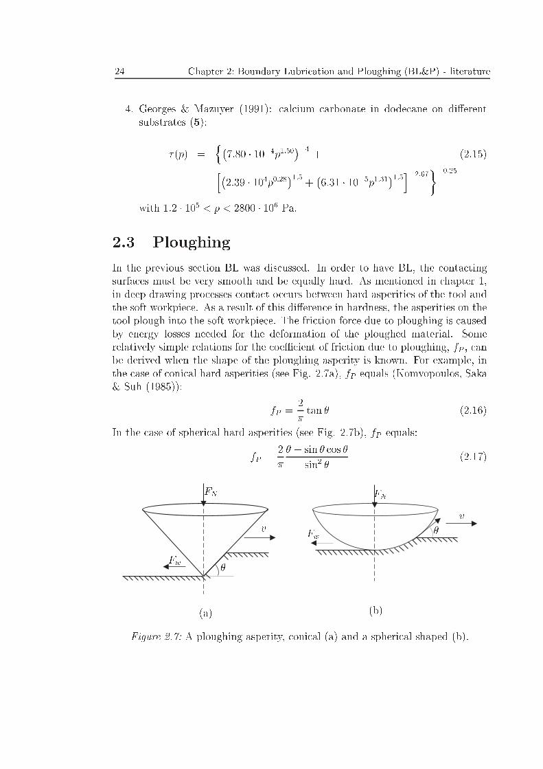
2.3 Ploughing
In the previous section BL was discussed. In order to have BL, the contactingsurfaces must be very smooth and be equally hard. As mentioned in chapter 1,in deep drawing processes contact occurs between hard asperities of the tool andthe soft workpiece. As a result of this di�erence in hardness, the asperities on thetool plough into the soft workpiece. The friction force due to ploughing is causedby energy losses needed for the deformation of the ploughed material. Somerelatively simple relations for the coeÆcient of friction due to ploughing, fP , canbe derived when the shape of the ploughing asperity is known. For example, inthe case of conical hard asperities (see Fig. 2.7a), fP equals (Komvopoulos, Saka& Suh (1985)):
fP =2
�tan � (2.16)
In the case of spherical hard asperities (see Fig. 2.7b), fP equals:
fP =2
�
� � sin � cos �
sin2 �(2.17)
(a) (b)
�
�
vv Fw
Fw
FNFN
Figure 2.7: A ploughing asperity, conical (a) and a spherical shaped (b).
2.4. Modelling BL&P - the Challen and Oxley model 25
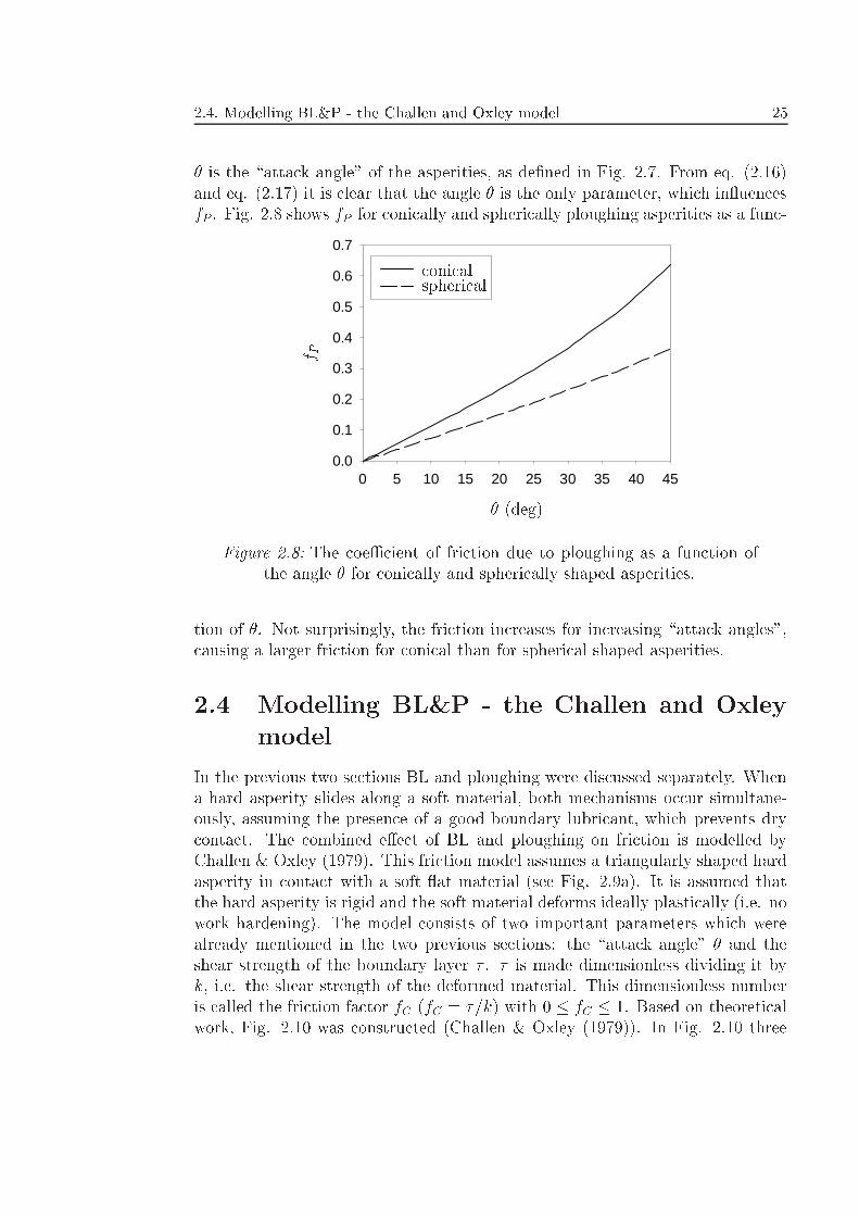
� is the \attack angle" of the asperities, as de�ned in Fig. 2.7. From eq. (2.16)and eq. (2.17) it is clear that the angle � is the only parameter, which in uencesfP . Fig. 2.8 shows fP for conically and spherically ploughing asperities as a func-
0 5 10 15 20 25 30 35 40 450.0
0.1
0.2
0.3
0.4
0.5
0.6
0.7
� (deg)
f P
conicalspherical
Figure 2.8: The coeÆcient of friction due to ploughing as a function ofthe angle � for conically and spherically shaped asperities.
tion of �. Not surprisingly, the friction increases for increasing \attack angles",causing a larger friction for conical than for spherical shaped asperities.
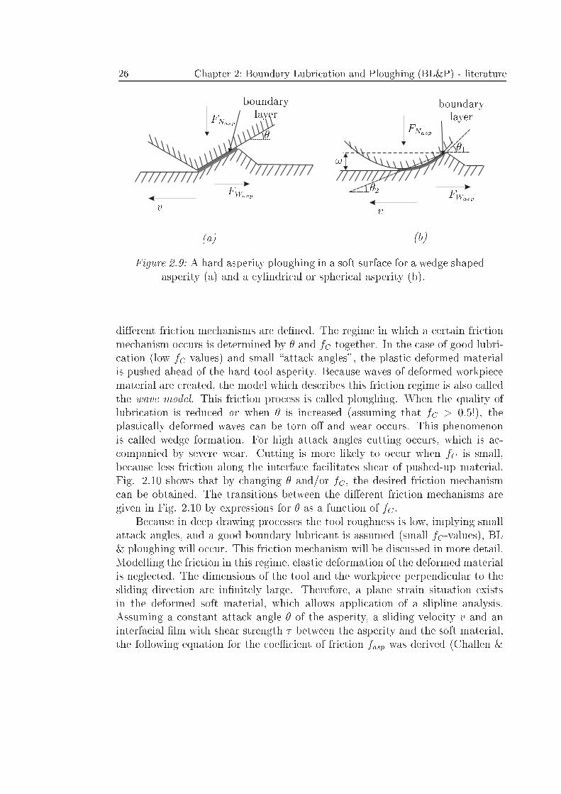
2.4 Modelling BL&P - the Challen and Oxley
model
In the previous two sections BL and ploughing were discussed separately. Whena hard asperity slides along a soft material, both mechanisms occur simultane-ously, assuming the presence of a good boundary lubricant, which prevents drycontact. The combined e�ect of BL and ploughing on friction is modelled byChallen & Oxley (1979). This friction model assumes a triangularly shaped hardasperity in contact with a soft at material (see Fig. 2.9a). It is assumed thatthe hard asperity is rigid and the soft material deforms ideally plastically (i.e. nowork hardening). The model consists of two important parameters which werealready mentioned in the two previous sections: the \attack angle" � and theshear strength of the boundary layer � . � is made dimensionless dividing it byk, i.e. the shear strength of the deformed material. This dimensionless numberis called the friction factor fC (fC = �=k) with 0 � fC � 1. Based on theoreticalwork, Fig. 2.10 was constructed (Challen & Oxley (1979)). In Fig. 2.10 three
26 Chapter 2: Boundary Lubrication and Ploughing (BL&P) - literature
�
boundarylayer
boundarylayer
!
FNasp
FNasp
�1
�2
vvFWasp
FWasp
(a) (b)
Figure 2.9: A hard asperity ploughing in a soft surface for a wedge shapedasperity (a) and a cylindrical or spherical asperity (b).
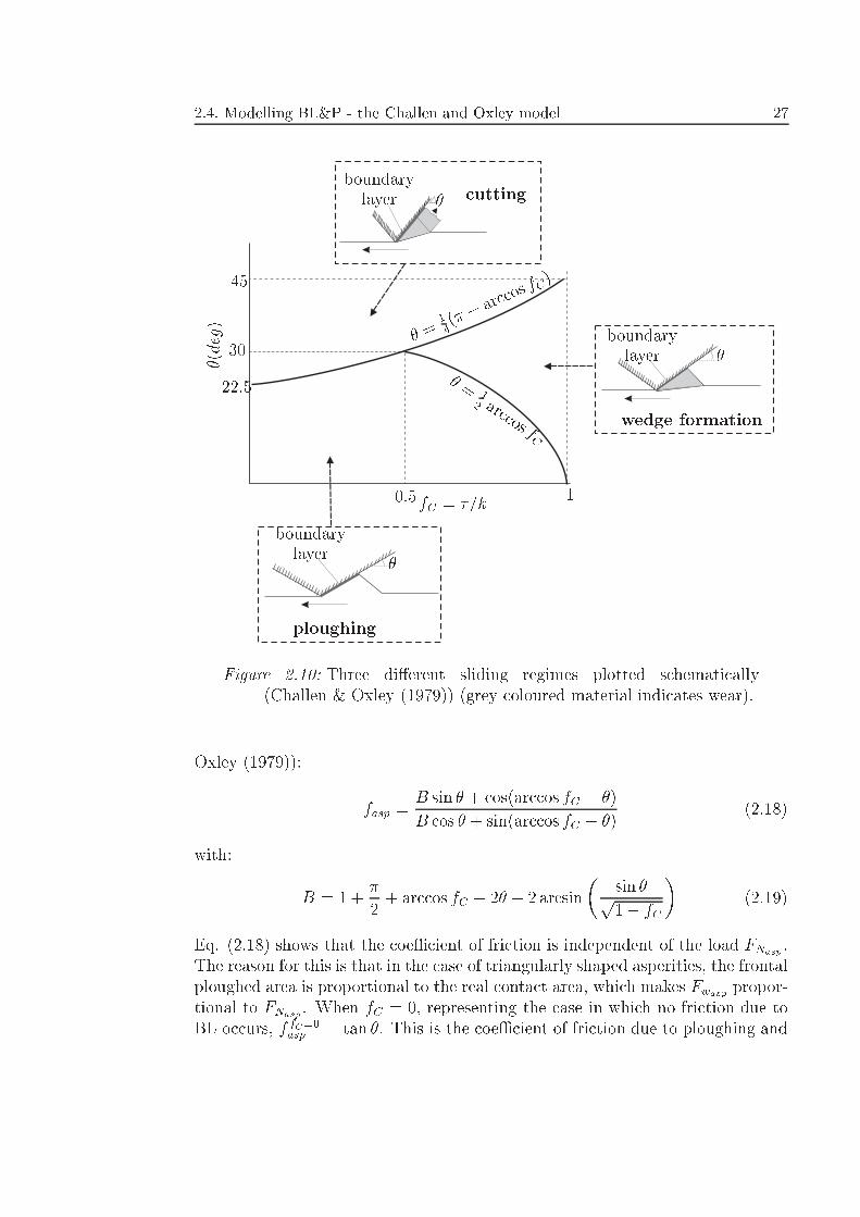
di�erent friction mechanisms are de�ned. The regime in which a certain frictionmechanism occurs is determined by � and fC together. In the case of good lubri-cation (low fC-values) and small \attack angles", the plastic deformed materialis pushed ahead of the hard tool asperity. Because waves of deformed workpiecematerial are created, the model which describes this friction regime is also calledthe wave model. This friction process is called ploughing. When the quality oflubrication is reduced or when � is increased (assuming that fC > 0:5!), theplastically deformed waves can be torn o� and wear occurs. This phenomenonis called wedge formation. For high attack angles cutting occurs, which is ac-companied by severe wear. Cutting is more likely to occur when fC is small,because less friction along the interface facilitates shear of pushed-up material.Fig. 2.10 shows that by changing � and/or fC , the desired friction mechanismcan be obtained. The transitions between the di�erent friction mechanisms aregiven in Fig. 2.10 by expressions for � as a function of fC .
Because in deep drawing processes the tool roughness is low, implying smallattack angles, and a good boundary lubricant is assumed (small fC-values), BL& ploughing will occur. This friction mechanism will be discussed in more detail.Modelling the friction in this regime, elastic deformation of the deformed materialis neglected. The dimensions of the tool and the workpiece perpendicular to thesliding direction are in�nitely large. Therefore, a plane strain situation existsin the deformed soft material, which allows application of a slipline analysis.Assuming a constant attack angle � of the asperity, a sliding velocity v and aninterfacial �lm with shear strength � between the asperity and the soft material,the following equation for the coeÆcient of friction fasp was derived (Challen &
2.4. Modelling BL&P - the Challen and Oxley model 27
� (deg)
boundarylayer
boundarylayer
boundarylayer
fC = �=k
ploughing
wedge formation
cutting
� =1
2 arccos fC
� =1
4(� �
arccos
fC)
0.5
30
22.5
1
45
�
�
�
Figure 2.10: Three di�erent sliding regimes plotted schematically(Challen & Oxley (1979)) (grey coloured material indicates wear).
Oxley (1979)):
fasp =B sin � + cos(arccos fC � �)
B cos � + sin(arccos fC � �)(2.18)
with:
B = 1 +�
2+ arccos fC � 2� � 2 arcsin
�sin �p1� fC
�(2.19)
Eq. (2.18) shows that the coeÆcient of friction is independent of the load FNasp .The reason for this is that in the case of triangularly shaped asperities, the frontalploughed area is proportional to the real contact area, which makes Fwasp propor-tional to FNasp. When fC = 0, representing the case in which no friction due toBL occurs, f fC=0asp = tan �. This is the coeÆcient of friction due to ploughing and
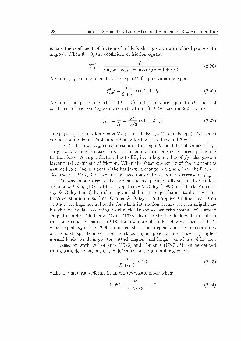
28 Chapter 2: Boundary Lubrication and Ploughing (BL&P) - literature
equals the coeÆcient of friction of a block sliding down an inclined plane withangle �. When � = 0, the coeÆcient of friction equals:
f �=0asp =fC
sin(arccos fC) + arccos fC + 1 + �=2(2.20)
Assuming fC having a small value, eq. (2.20) approximately equals:
f �=0asp =fC
2 + �� 0:194 � fC (2.21)
Assuming no ploughing e�ects (� = 0) and a pressure equal to H, the realcoeÆcient of friction fBL as measured with an SFA (see section 2.2) equals:
fBL =�
H=
fC
3p3� 0:192 � fC (2.22)
In eq. (2.22) the relation k = H=3p3 is used. Eq. (2.21) equals eq. (2.22) which
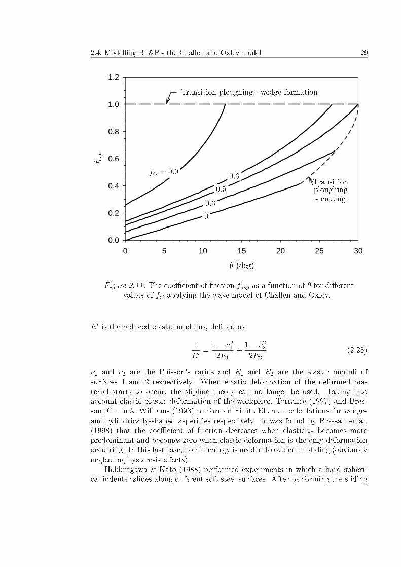
veri�es the model of Challen and Oxley for low fC values and � = 0.Fig. 2.11 shows fasp as a function of the angle � for di�erent values of fC .
Larger attack angles cause larger coeÆcients of friction due to larger ploughingfriction force. A larger friction due to BL, i.e. a larger value of fC , also gives alarger total coeÆcient of friction. When the shear strength � of the lubricant isassumed to be independent of the hardness, a change in k also a�ects the friction.Because k = H=3
p3, a harder workpiece material results in a decrease of fasp.
The wave model discussed above, has been experimentally veri�ed by Challen,McLean & Oxley (1984), Black, Kopalinsky & Oxley (1988) and Black, Kopalin-sky & Oxley (1990) by indenting and sliding a wedge shaped tool along a lu-bricated aluminium surface. Challen & Oxley (1984) applied slipline theories oncontacts for high normal loads, for which interaction occurs between neighbour-ing slipline �elds. Assuming a cylindrically shaped asperity instead of a wedgeshaped asperity, Challen & Oxley (1983) deduced slipline �elds which result inthe same equation as eq. (2.18) for low normal loads. However, the angle �,which equals �2 in Fig. 2.9b, is not constant, but depends on the penetration !of the hard asperity into the soft surface. Higher penetrations, caused by highernormal loads, result in greater \attack angles" and larger coeÆcients of friction.
Based on work by Torrance (1996) and Torrance (1997), it can be derivedthat elastic deformations of the deformed material dominate when:
H
E 0 tan �> 1:7 (2.23)
while the material deforms in an elastic-plastic mode when:
0:085 <H
E 0 tan �< 1:7 (2.24)
2.4. Modelling BL&P - the Challen and Oxley model 29
0 5 10 15 20 25 300.0
0.2
0.4
0.6
0.8
1.0
1.2
� (deg)
f asp
fC = 0:9
0
0.3
0.5
0.6
Transition ploughing - wedge formation
Transitionploughing- cutting
Figure 2.11: The coeÆcient of friction fasp as a function of � for di�erentvalues of fC applying the wave model of Challen and Oxley.
E 0 is the reduced elastic modulus, de�ned as
1
E 0=
1� �212E1
+1� �222E2
(2.25)
�1 and �2 are the Poisson's ratios and E1 and E2 are the elastic moduli ofsurfaces 1 and 2 respectively. When elastic deformation of the deformed ma-terial starts to occur, the slipline theory can no longer be used. Taking intoaccount elastic-plastic deformation of the workpiece, Torrance (1997) and Bres-san, Genin & Williams (1998) performed Finite Element calculations for wedge-and cylindrically-shaped asperities respectively. It was found by Bressan et al.(1998) that the coeÆcient of friction decreases when elasticity becomes morepredominant and becomes zero when elastic deformation is the only deformationoccurring. In this last case, no net energy is needed to overcome sliding (obviouslyneglecting hysteresis e�ects).
Hokkirigawa & Kato (1988) performed experiments in which a hard spheri-cal indenter slides along di�erent soft steel surfaces. After performing the sliding
30 Chapter 2: Boundary Lubrication and Ploughing (BL&P) - literature
experiments, the wear mode (ploughing, wedge formation or cutting) was deter-mined. Applying the de�nition � = �1 (see Fig. 2.9), a good agreement was foundwith Fig. 2.10, which proves that eq. (2.18) may also be applied for sphericalasperities.
2.5 Summary
In this chapter a review was presented of the literature regarding friction dueto Boundary Lubrication (BL) and Ploughing. It is shown that the friction ofboundary layers depends strongly on the applied pressure, the sliding speed andthe temperature. In general, the in uence of the pressure and the temperature onthe shear strength is largely similar for di�erent boundary layers. An increase ofthe pressure causes an increase of the shear strength while an increase of the tem-perature lowers the shear strength. However, the in uence of the speed dependson the type of lubricant. Fits are constructed, which describe the dependence ofthe shear strength of boundary layers on these parameters.
The in uence of the ploughing force is mainly determined by the hardness ofthe ploughed material (not for wedge shaped ploughing asperities) and the shapeof the ploughing asperity. Sharper ploughing asperities and a softer ploughedmaterial will lead to larger coeÆcients of friction. Both friction mechanisms areincluded in a friction model developed by Challen & Oxley (1979). This model,which describes the contact between one single ploughing asperity and a softmaterial, will be used in a macroscopic friction model with application to deepdrawing. First, a contact model for deep drawing is needed, which will be derivedin chapter 3.
Chapter 3
A newly developed contact model
In chapter 1 the contact regions between the tool and the workpiece in deepdrawing were discussed. A characteristic of these processes is the contact betweena hard smooth surface (the tool) and a soft rough surface (the workpiece). In sucha contact, the asperities of the soft workpiece are attened by the hard tool anda real contact area develops. The extent of attening depends on operationalparameters such as the normal load and the bulk strain, material parameterssuch as the hardness of the workpiece and roughness parameters. Contact modelsquantitatively describe the in uence of these parameters on the real contact area.
In this chapter a new contact model is presented, which is applicable to deepdrawing processes. The �rst section gives a short summary of contact modelspublished in the literature. In the second section a new contact model is derivedfor ideal plastically deforming asperities. In the third section this model is ex-tended by introducing work hardening e�ects. The fourth section deals with thein uence of the bulk strain on the contact behaviour. In section �ve the in uenceof shear strength on the real contact area is discussed. Finally, the conclusionsand a summary of this chapter are given in section six.
3.1 Overview of contact models
In the literature many contact models have been published which describe thecontact between two rough surfaces. A recent review was made by Liu, Wang &Lin (1999). The majority of models consider the contact between a hard perfectlysmooth surface and a soft rough surface. This is also assumed here. The modeof asperity deformation of the soft rough surface may be elastic, plastic or acombination. If ideal plastic deformation occurs, the real pressure in an asperityequals the hardness, if work hardening of the asperities occurs, the real pressurein an asperity is a function of the extent of deformation. A summary of somecontact models will be given now.
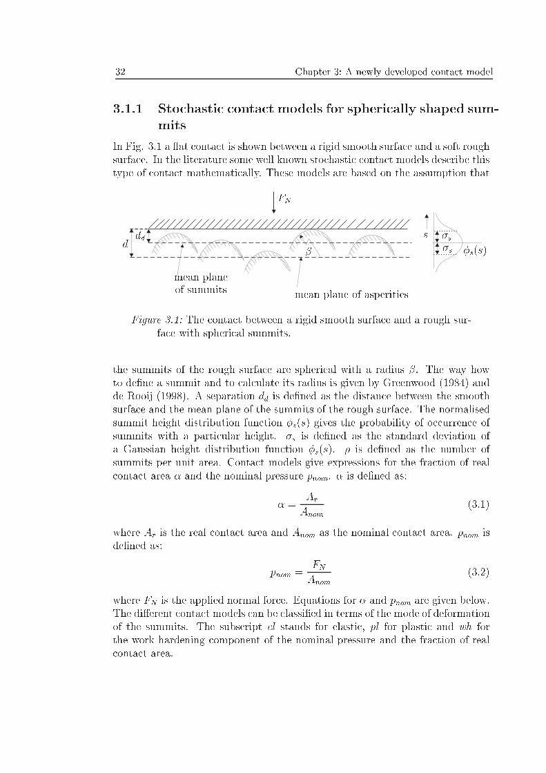
32 Chapter 3: A newly developed contact model
3.1.1 Stochastic contact models for spherically shaped sum-mits
In Fig. 3.1 a at contact is shown between a rigid smooth surface and a soft roughsurface. In the literature some well known stochastic contact models describe thistype of contact mathematically. These models are based on the assumption that
�
mean plane of asperities
mean planeof summits
�s(s)
s
FN
dd�s
�sd
Figure 3.1: The contact between a rigid smooth surface and a rough sur-face with spherical summits.
the summits of the rough surface are spherical with a radius �. The way howto de�ne a summit and to calculate its radius is given by Greenwood (1984) andde Rooij (1998). A separation dd is de�ned as the distance between the smoothsurface and the mean plane of the summits of the rough surface. The normalisedsummit height distribution function �s(s) gives the probability of occurrence ofsummits with a particular height. �s is de�ned as the standard deviation ofa Gaussian height distribution function �s(s). � is de�ned as the number ofsummits per unit area. Contact models give expressions for the fraction of realcontact area � and the nominal pressure pnom. � is de�ned as:
� =ArAnom
(3.1)
where Ar is the real contact area and Anom as the nominal contact area. pnom isde�ned as:
pnom =FNAnom
(3.2)
where FN is the applied normal force. Equations for � and pnom are given below.The di�erent contact models can be classi�ed in terms of the mode of deformationof the summits. The subscript el stands for elastic, pl for plastic and wh forthe work hardening component of the nominal pressure and the fraction of realcontact area.
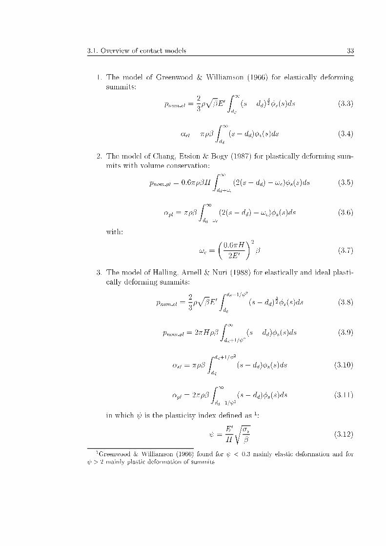
3.1. Overview of contact models 33
1. The model of Greenwood & Williamson (1966) for elastically deformingsummits:
pnom el =2
3�p�E 0
Z 1
dd
(s� dd)3
2�s(s)ds (3.3)
�el = ���
Z 1
dd
(s� dd)�s(s)ds (3.4)
2. The model of Chang, Etsion & Bogy (1987) for plastically deforming sum-mits with volume conservation:
pnom pl = 0:6���H
Z 1
dd+!c
(2(s� dd)� !c)�s(s)ds (3.5)
�pl = ���
Z 1
dd+!c
(2(s� dd)� !c)�s(s)ds (3.6)
with:
!c =
�0:6�H
2E 0
�2
� (3.7)
3. The model of Halling, Arnell & Nuri (1988) for elastically and ideal plasti-cally deforming summits:
pnom el =2
3�p�E 0
Z dd+1= 2
dd
(s� dd)3
2�s(s)ds (3.8)
pnom pl = 2�H��
Z 1
dd+1= 2(s� dd)�s(s)ds (3.9)
�el = ���
Z dd+1= 2
dd
(s� dd)�s(s)ds (3.10)
�pl = 2���
Z 1
dd+1= 2(s� dd)�s(s)ds (3.11)
in which is the plasticity index de�ned as 1:
=E 0
H
r�s�
(3.12)
1Greenwood & Williamson (1966) found for < 0:3 mainly elastic deformation and for > 2 mainly plastic deformation of summits
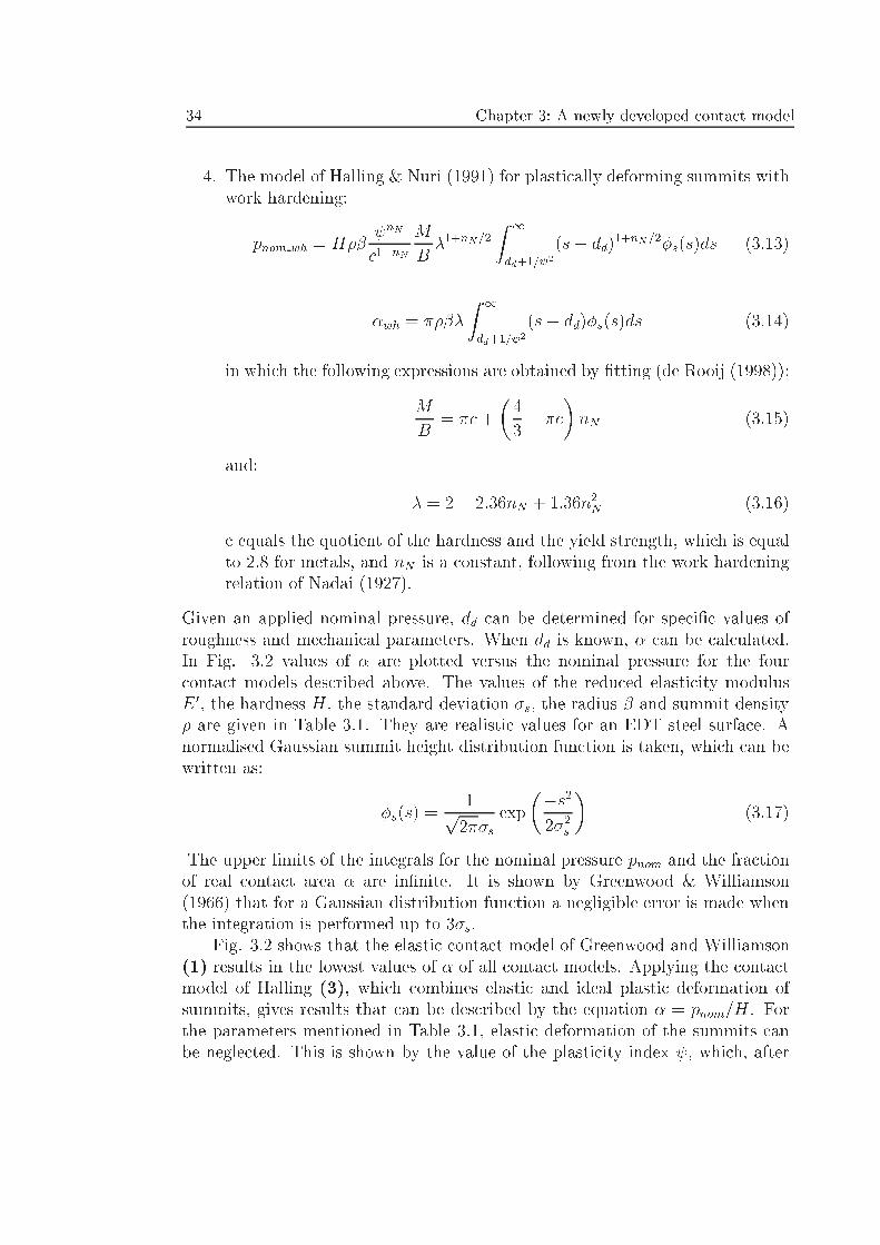
34 Chapter 3: A newly developed contact model
4. The model of Halling & Nuri (1991) for plastically deforming summits withwork hardening:
pnom wh = H�� nN
c1�nNM
B�1+nN=2
Z 1
dd+1= 2(s� dd)
1+nN=2�s(s)ds (3.13)
�wh = ����
Z 1
dd+1= 2(s� dd)�s(s)ds (3.14)
in which the following expressions are obtained by �tting (de Rooij (1998)):
M
B= �c+
�4
3� �c
�nN (3.15)
and:
� = 2� 2:36nN + 1:36n2N (3.16)
c equals the quotient of the hardness and the yield strength, which is equalto 2.8 for metals, and nN is a constant, following from the work hardeningrelation of Nadai (1927).
Given an applied nominal pressure, dd can be determined for speci�c values ofroughness and mechanical parameters. When dd is known, � can be calculated.In Fig. 3.2 values of � are plotted versus the nominal pressure for the fourcontact models described above. The values of the reduced elasticity modulusE 0, the hardness H, the standard deviation �s, the radius � and summit density� are given in Table 3.1. They are realistic values for an EDT steel surface. Anormalised Gaussian summit height distribution function is taken, which can bewritten as:
�s(s) =1p2��s
exp
��s22�2s
�(3.17)
The upper limits of the integrals for the nominal pressure pnom and the fractionof real contact area � are in�nite. It is shown by Greenwood & Williamson(1966) that for a Gaussian distribution function a negligible error is made whenthe integration is performed up to 3�s.
Fig. 3.2 shows that the elastic contact model of Greenwood and Williamson(1) results in the lowest values of � of all contact models. Applying the contactmodel of Halling (3), which combines elastic and ideal plastic deformation ofsummits, gives results that can be described by the equation � = pnom=H. Forthe parameters mentioned in Table 3.1, elastic deformation of the summits canbe neglected. This is shown by the value of the plasticity index , which, after
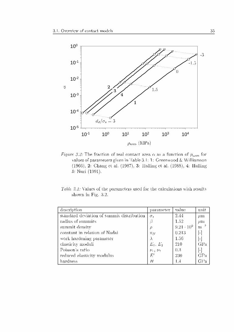
3.1. Overview of contact models 35
10-1 100 101 102 103 10410-5
10-4
10-3
10-2
10-1
100
pnom (MPa)
�
1
23
4
dd=�s = 3
1.5
0
-1.5
-3
Figure 3.2: The fraction of real contact area � as a function of pnom forvalues of parameters given in Table 3.1; 1: Greenwood &Williamson(1966), 2: Chang et al. (1987), 3: Halling et al. (1988), 4: Halling& Nuri (1991).
Table 3.1: Values of the parameters used for the calculations with resultsshown in Fig. 3.2.
description parameter value unitstandard deviation of summit distribution �s 2.44 �mradius of summits � 1.52 �msummit density � 9:21 � 109 m�2
constant in relation of Nadai nN 0.213 [-]work hardening parameter � 1.56 [-]elasticity moduli E1, E2 210 GPaPoisson's ratio �1, �2 0.3 [-]reduced elasticity modulus E 0 230 GPahardness H 1.4 GPa
36 Chapter 3: A newly developed contact model
substituting the values of the parameters given in Table 3.1, takes the value of208. Because this value is much larger than 2, plastic deformation dominates(Greenwood & Williamson (1966)).
If work hardening is taken into account (4), � becomes smaller than in thecase of ideal plastic deformation, because work hardening causes more resistanceagainst deformation. The plasticity model of Chang (2) gives the highest valuesof �. This is because Chang assumes the beginning of plasticity at a lower valueof the pressure in an asperity (i.e., 0:6 � H). The results from application ofChang's model can be described by the equation � = pnom=(0:6 �H).
Fig. 3.2 also shows points in the graph for which dd=�s equals -3 (i.e. whenall summits are in contact), -1.5, 0, 1.5 and 3 (i.e. no contact). When dd=�sequals -3, i.e. the situation of total contact, the theoretical value of � is notequal to 1, which is, of course, not realistic. Also, these contact models do notacount for the interaction between neighbouring asperities, which causes a lessthan proportionally increasing value of �. Concluding, these stochastic modelsare only valid for loads under which interactions between neighbouring asperitiesdo not occur (see also section 3.1.4).
3.1.2 Numerical contact models
Numerical contact models have been developed by, for example, Webster & Sayles(1986), Liang & Linqing (1991) and Lee (1996). These models mathematicallydescribe the contact between a smooth and a rough surface by considering theasperities as bars. Equations are applied which relate the displacement of anasperity to the pressure occurring in the asperities. In all these models elasticdisplacements of asperities are assumed. For plastic displacements, no such ex-pressions exist. Therefore, these models are not suitable for application in deepdrawing processes, because plastic deformations dominate in these processes.
3.1.3 Contact models including bulk deformation
A characteristic feature of deep drawing is bulk deformation. Bulk deformationhas an important e�ect on the attening and roughening of a surface. Contactmodels, which take this e�ect into account were developed by Wilson & Sheu(1988), Sutcli�e (1988) and Kimura & Childs (1999) for wedge-shaped asperitieswith an equal height. Numerical calculations, which show the e�ect of bulk defor-mation on attening, were performed by Ike & Makinouchi (1990) and Korzekwa,Dawson & Wilson (1992). In section 3.4 the e�ect of bulk deformation is treatedin more detail.
3.1. Overview of contact models 37
3.1.4 Contact models including volume conservation
It is experimentally shown by Pullen & Williamson (1972) that when the nominalpressure pnom is larger than 0:3 �H, the fraction of real contact area � increasesless than proportionally with the nominal pressure pnom. Uppal & Probert (1973)found non-linearity between � and pnom for nominal pressures larger than 0:025 �H.
When it is assumed that the volume of the indented asperities equals thevolume of the rising valleys, Pullen & Williamson (1972) derived the followingrelation between pnom=H and �:
pnom=H =�
1� �(3.18)
In contrast to the stochastic contact models, derived for summits, the modeldeveloped by Pullen & Williamson (1972) is valid for surface asperities. A sepa-ration d is introduced as the distance between the smooth surface and the meanplane of the surface asperities. �(z) is the normalised surface asperity heightdistribution function and U is the constant rise of the valleys. The separation dand the rise U can be obtained from:
� =
Z 1
d�U
�(z)dz (3.19)
and:
U =
Z 1
d�U
(z � d+ U)�(z)dz (3.20)
This plastic contact model of Williamson and Pullen is valid for arbitrarily shapedasperities. However, the model shows some important shortcomings:
� It does not account for asperity persistence (i.e. the resistance against de-formation at higher loads). This phenomenon was �rst discovered by Moore(1948). He found that contrary to expectations the application of a largenormal load to a rough aluminium material did not atten all asperities.The fraction of real contact area was lower than predicted by the idealplastic contact theory. This means that the real pressure pr, occurring inthe indented asperities, was higher than the hardness and in fact increasedduring indentation, because pr = pnom=�. Similar observations have beenreported by Williamson & Hunt (1972), Uppal & Probert (1973), Childs(1973) and Chivers, Mitchell & Rowe (1974). Because persistence also oc-curred for non-work hardening materials, it cannot be only explained by theoccurrence of work hardening. The phenomenon is still not well understoodand a good analytical method to describe asperity persistence does not yetexist.
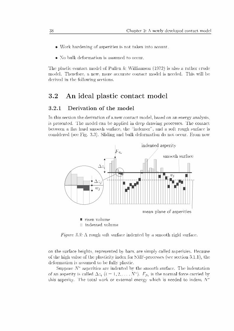
38 Chapter 3: A newly developed contact model
� Work hardening of asperities is not taken into acount.
� No bulk deformation is assumed to occur.
The plastic contact model of Pullen & Williamson (1972) is also a rather crudemodel. Therefore, a new, more accurate contact model is needed. This will bederived in the following sections.
3.2 An ideal plastic contact model
3.2.1 Derivation of the model
In this section the derivation of a new contact model, based on an energy analysis,is presented. The model can be applied in deep drawing processes. The contactbetween a at hard smooth surface, the \indenter", and a soft rough surface isconsidered (see Fig. 3.3). Sliding and bulk deformation do not occur. From now
mean plane of asperities
smooth surface
indented asperity
�zi
uj
FNi
�zjwj
indented volumerisen volume
Figure 3.3: A rough soft surface indented by a smooth rigid surface.
on the surface heights, represented by bars, are simply called asperities. Becauseof the high value of the plasticity index for SMF-processes (see section 3.1.1), thedeformation is assumed to be fully plastic.
Suppose N� asperities are indented by the smooth surface. The indentationof an asperity is called �zi (i = 1; 2; : : : ; N�). FNi
is the normal force carried bythis asperity. The total work or external energy which is needed to indent N�
3.2. An ideal plastic contact model 39
asperities amounts to:
WN�
ext =N�Xi=1
FNi�zi (3.21)
It is now assumed that, due to the indentation of N� asperities, the remainingnon-indented asperities rise. The physical explanation of this is presented inappendix A, where an analogy is drawn with the plane strain compression test.Due to the rise, new asperities will contact with the \indenter", as is shown inFig. 3.3. The number of asperities in contact with the indenter due to the riseonly is called N��. It is assumed that if these asperities were not in contact withthe indenter, they would rise by a distance uj with j = 1; 2; : : : ; N��. However,because this rise uj is restricted by the presence of the \indenter", the asperitiesactually rise a distance wj (wj � uj). An amount of workWN��
ext must be deliveredto prevent a rise �zj = uj�wj and keep the rising asperities below the \indenter".WN��
ext is given by:
WN��
ext =N��Xj=1
FNj�zj (3.22)
The total amount of work or external energy Wext is obtained by adding WN�
ext
(eq. (3.21)) to WN��
ext (eq. (3.22)), resulting in:
Wext =NXk=1
FNk�zk (3.23)
N is the total number of asperities in contact with the indenter (N = N�+N��).Without making further assumptions, eq. (3.23) can be written as:
Wext = �1FNd�zk with 0 < �1 � 1 (3.24)
where d�zk is the maximum indentation of the rough surface and:
�1 =
NPk=1
FNk�zk
d�zk NPk=1
FNk
=
NPk=1
FNk�zk
d�zkFN (3.25)
�1 may be regarded as some kind of energy factor, because it in uences the amountof external energy which must be delivered to indent a rough surface.
The external energy which is applied to indent the surface is used for two physical
40 Chapter 3: A newly developed contact model
mechanisms. One part of the energy will be absorbed by the indented surface.The remaining part will be used to lift up the valleys. Because of the energy bal-ance, the external energy Wext must equal the internal energy Wint. With Wintst
as the amount of absorbed energy and Wintri as the energy needed for raising thevalleys, this yields:
Wint = Wintst +Wintri (3.26)
The area of an asperity is equal to �A with all asperities having the same area.Because ideal plastic deformation is assumed, the real pressure in the indentedasperities equals the hardness H. Thus, Wintst, the absorbed energy, can bewritten as:
Wintst =NXk=1
H�A�zk (3.27)
In eq. (3.27) the summation is performed over the number of indented asperitiesN . This means that energy is only dissipated in the indented asperities. Intro-ducing the constant �2 (0 < �2 � 1) and writing N �A = Ar (Ar is the realcontact area), eq. (3.27) can be written as:
Wintst = �2HArd�zk (3.28)
with
�2 =
NPk=1
�zk
Nd�zk (3.29)
The parameter �2 is called a shape factor, because it is in uenced by the distri-bution of the asperities or the \shape" of the surface.
An equation for Wintri is required now. A parameter � is introduced, whichdetermines the amount of energy which is needed to lift up the valleys. � iscalled the asperity persistence parameter or simply the persistence parameter.Wintri can be written as the sum of the energy needed to raise N�� asperities,which touch the \indenter" after application of the normal load, and the energyneeded to raise M asperities, which are not in contact with the \indenter":
Wintri = �
MXm=1
umH�A+N��Xj=1
H�Awj
!(3.30)
When � = 0, no energy is needed to raise the valleys. A negative value of �implies that energy is released when the valleys rise, which is unlikely to happen.
3.2. An ideal plastic contact model 41
When � = 1, a maximum amount of energy must be delivered to lift up thevalleys. Concluding, 0 � � � 1.
The parameter � in uences the extent of asperity interaction or persistence.According to Childs (1977), persistence increases during an increase of the nor-mal load. Childs (1977) de�ned asperity persistence as \an increasing diÆcultyof \extruding" material through the gaps between the plastically compressed realareas of contact". In this way � will increase when the normal load is increased.More attention is paid to the in uence of the persistence parameter � on themodel in section 3.2.2.
Eq. (3.30) is considered. The following stochastic variables are introduced (seealso Fig. 3.4):
� u(z): the rise of the asperities which may be a function of the height of theasperities z.
� �(z): the normalised height distribution function of the asperities of therough surface.
� d: the separation, i.e. the distance between the indenter and the meanplane of the asperities of the rough surface.
� z1: the minimum height of an asperity, which comes into contact with thesmooth surface after application of the normal load. z1 can be obtainedfrom the condition:
z1 + u(z1) = d (3.31)
Using these variables eq. (3.30) can be written as:
Wintri = �HAnom
�Z d
�1
u(z)�(z)dz �Z d
z1
(z � z1)�(z)dz
�(3.32)
In eq. (3.32) d and u(z) are unknown parameters. Therefore, more equations areneeded. A second equation can be obtained by assuming volume conservation.Volume conservation applies when plastic deformation occurs. Applying volumeconservation and writing the equation in a deterministic way, leads to (see alsoFig. 3.3 and Fig. 3.4):
MXm=1
um�A| {z }V"1
+N��Xj=1
wj�A| {z }V"2
=N�Xj=1
�zj�A| {z }V#
(3.33)
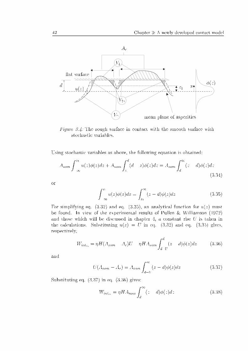
42 Chapter 3: A newly developed contact model
V#
V"2
V"1
d z1
Ar
�(z)
mean plane of asperities
u(z)
at surface
z
Figure 3.4: The rough surface in contact with the smooth surface withstochastic variables.
Using stochastic variables as above, the following equation is obtained:
Anom
Z z1
�1
u(z)�(z)dz + Anom
Z d
z1
(d� z)�(z)dz = Anom
Z 1
d
(z � d)�(z)dz
(3.34)
or Z z1
�1
u(z)�(z)dz =
Z 1
z1
(z � d)�(z)dz (3.35)
For simplifying eq. (3.32) and eq. (3.35), an analytical function for u(z) mustbe found. In view of the experimental results of Pullen & Williamson (1972)and those which will be discussed in chapter 4, a constant rise U is taken inthe calculations. Substituting u(z) = U in eq. (3.32) and eq. (3.35) gives,respectively,
Wintri = �H(Anom � Ar)U � �HAnom
Z d
d�U
(z � d)�(z)dz (3.36)
and
U(Anom � Ar) = Anom
Z 1
d�U
(z � d)�(z)dz (3.37)
Substituting eq. (3.37) in eq. (3.36) gives:
Wintri = �HAnom
Z 1
d
(z � d)�(z)dz (3.38)
3.2. An ideal plastic contact model 43
In eq. (3.38) the separation d is the only variable which is unknown. For reasonsof convenience, eq. (3.38) is written in a deterministic way:
Wintri = �H
N�Xi=1
�zi�A (3.39)
Assuming d�zk equals d�zi with k = 1; : : : ; N and i = 1; : : : ; N�, eq. (3.39) canbe written as:
Wintri = ��3H(Ar �N���A)d�zk (3.40)
with
�3 =
N�Pi=1
�zi
N�d�zk (3.41)
Similar to �2 (eq. (3.29)), �3 can be regarded as a shape factor. Substituting eq.(3.40) and eq. (3.28) in eq. (3.26) and equalling to eq. (3.24) gives:
FNH
=�2�1Ar +
�3�1� (Ar �N���A) (3.42)
The parameters �1, �2 and �3 can be expressed as a function of each other. Inappendix B it is shown that:
�2 =�
��1 (3.43)
with:
� =ArAnom
=
Z 1
d�U
�(z)dz (3.44)
and:
� =
Z 1
d�U
FN(z)�(z)dz ��Z d
d�U
(z + U � d)�(z)dz +
Z 1
d
(z � d)�(z)dz
�Z d
d�U
FN(z)(z + U � d)�(z)dz +
Z 1
d
FN (z)(z � d)�(z)dz
(3.45)
FN(z) is the normal force acting on an asperity with height z. � is determinedby FN(z), �(z), the separation d and the rise U. Appendix B also shows that�2 � �1, which gives 0 < � � �. The relation between �3 and �2 is:
�3 = � � �2 � c(d; U) (3.46)
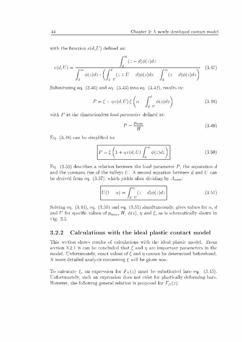
44 Chapter 3: A newly developed contact model
with the function c(d; U) de�ned as:
c(d; U) =
Z 1
d
(z � d)�(z)dzZ 1
d
�(z)dz ��Z d
d�U
(z + U � d)�(z)dz +
Z 1
d
(z � d)�(z)dz
� (3.47)
Substituting eq. (3.46) and eq. (3.43) into eq. (3.42), results in:
P = � + � c(d; U) �
���
Z d
d�U
�(z)dz
�(3.48)
with P as the dimensionless load parameter de�ned as:
P =pnomH
(3.49)
Eq. (3.48) can be simpli�ed to:
P = �
�1 + � c(d; U)
Z 1
d
�(z)dz
�(3.50)
Eq. (3.50) describes a relation between the load parameter P , the separation dand the constant rise of the valleys U . A second equation between d and U canbe derived from eq. (3.37), which yields after dividing by Anom:
U(1� �) =
Z 1
d�U
(z � d)�(z)dz (3.51)
Solving eq. (3.44), eq. (3.50) and eq. (3.51) simultaneously, gives values for �, dand U for speci�c values of pnom, H, �(z), � and �, as is schematically shown inFig. 3.5.
3.2.2 Calculations with the ideal plastic contact model
This section shows results of calculations with the ideal plastic model. Fromsection 3.2.1 it can be concluded that � and � are important parameters in themodel. Unfortunately, exact values of � and � cannot be determined beforehand.A more detailed analysis concerning � will be given now.
To calcutate �, an expression for FN(z) must be substituted into eq. (3.45).Unfortunately, such an expression does not exist for plastically deforming bars.However, the following general relation is proposed for FN(z):
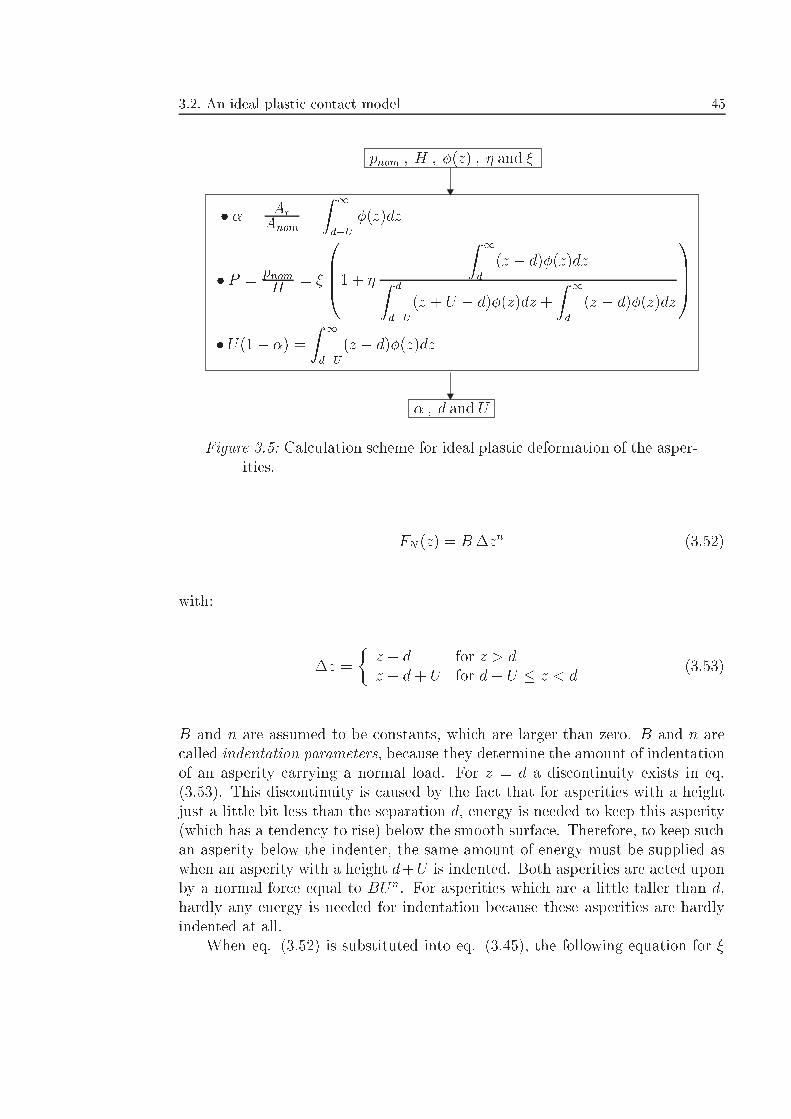
3.2. An ideal plastic contact model 45
pnom ; H ; �(z) ; � and �
� � = ArAnom
=
Z 1
d�U
�(z)dz
� P = pnomH = �
0BB@1 + �
Z 1
d
(z � d)�(z)dzZ d
d�U
(z + U � d)�(z)dz +
Z 1
d
(z � d)�(z)dz
1CCA� U(1� �) =
Z 1
d�U
(z � d)�(z)dz
� ; d and U
Figure 3.5: Calculation scheme for ideal plastic deformation of the asper-ities.
FN (z) = B�zn (3.52)
with:
�z =
�z � d for z > dz � d+ U for d� U � z < d
(3.53)
B and n are assumed to be constants, which are larger than zero. B and n arecalled indentation parameters, because they determine the amount of indentationof an asperity carrying a normal load. For z = d a discontinuity exists in eq.(3.53). This discontinuity is caused by the fact that for asperities with a heightjust a little bit less than the separation d, energy is needed to keep this asperity(which has a tendency to rise) below the smooth surface. Therefore, to keep suchan asperity below the indenter, the same amount of energy must be supplied aswhen an asperity with a height d+U is indented. Both asperities are acted uponby a normal force equal to BUn. For asperities which are a little taller than d,hardly any energy is needed for indentation because these asperities are hardlyindented at all.
When eq. (3.52) is substituted into eq. (3.45), the following equation for �
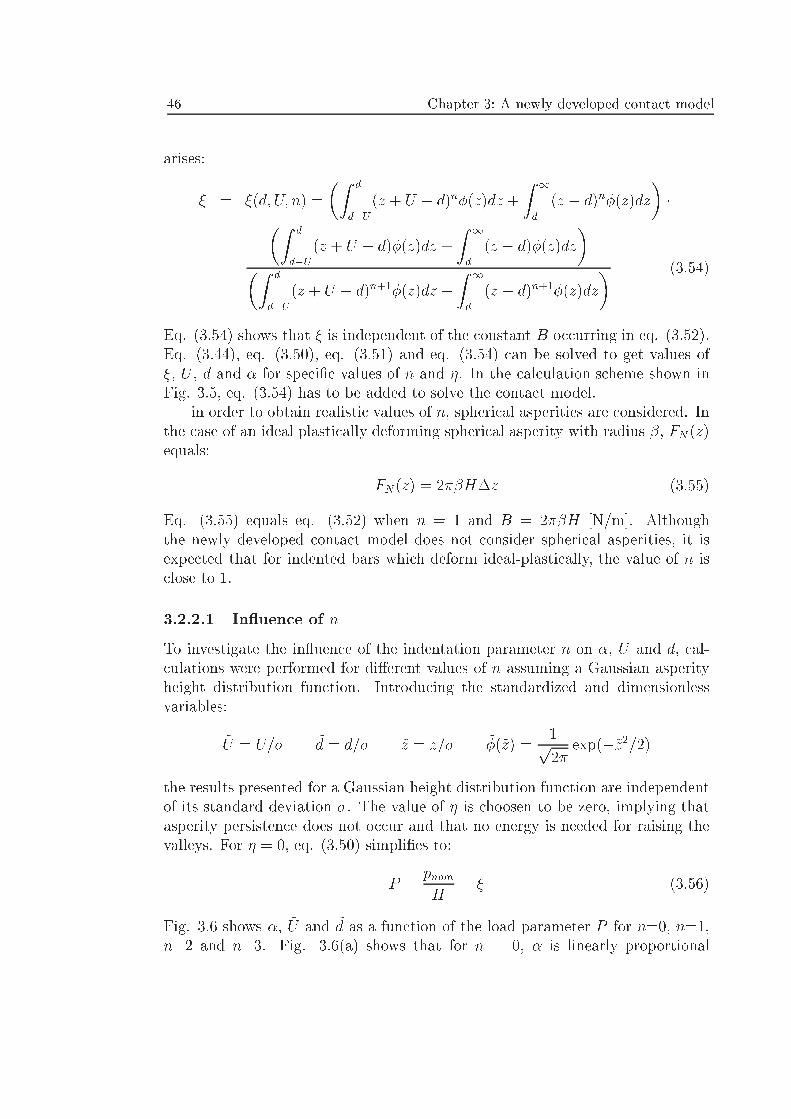
46 Chapter 3: A newly developed contact model
arises:
� = �(d; U; n) =
�Z d
d�U
(z + U � d)n�(z)dz +
Z 1
d
(z � d)n�(z)dz
���Z d
d�U
(z + U � d)�(z)dz +
Z 1
d
(z � d)�(z)dz
��Z d
d�U
(z + U � d)n+1�(z)dz +
Z 1
d
(z � d)n+1�(z)dz
� (3.54)
Eq. (3.54) shows that � is independent of the constant B occurring in eq. (3.52).Eq. (3.44), eq. (3.50), eq. (3.51) and eq. (3.54) can be solved to get values of�, U , d and � for speci�c values of n and �. In the calculation scheme shown inFig. 3.5, eq. (3.54) has to be added to solve the contact model.
in order to obtain realistic values of n, spherical asperities are considered. Inthe case of an ideal plastically deforming spherical asperity with radius �, FN (z)equals:
FN(z) = 2��H�z (3.55)
Eq. (3.55) equals eq. (3.52) when n = 1 and B = 2��H [N/m]. Althoughthe newly developed contact model does not consider spherical asperities, it isexpected that for indented bars which deform ideal-plastically, the value of n isclose to 1.
3.2.2.1 In uence of n
To investigate the in uence of the indentation parameter n on �, U and d, cal-culations were performed for di�erent values of n assuming a Gaussian asperityheight distribution function. Introducing the standardized and dimensionlessvariables:
~U = U=� ~d = d=� ~z = z=� ~�(~z) =1p2�
exp(�~z2=2)
the results presented for a Gaussian height distribution function are independentof its standard deviation �. The value of � is choosen to be zero, implying thatasperity persistence does not occur and that no energy is needed for raising thevalleys. For � = 0, eq. (3.50) simpli�es to:
P =pnomH
= � (3.56)
Fig. 3.6 shows �, ~U and ~d as a function of the load parameter P for n=0, n=1,n=2 and n=3. Fig. 3.6(a) shows that for n = 0, � is linearly proportional
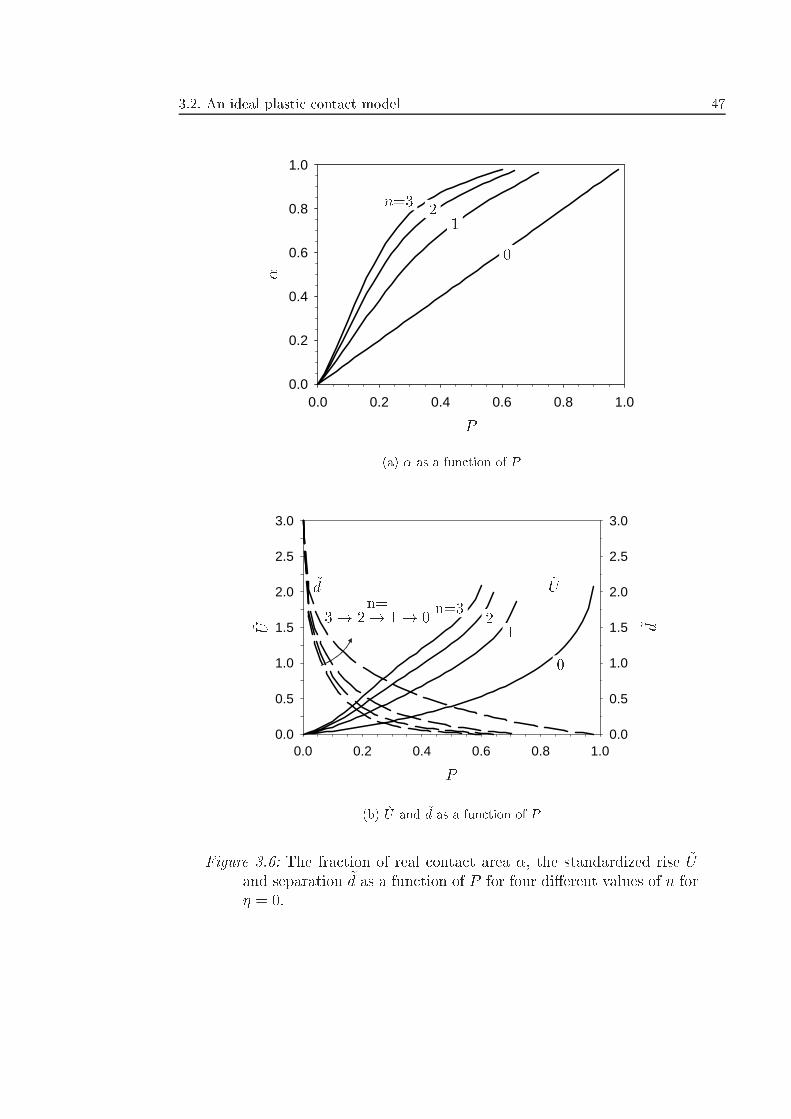
3.2. An ideal plastic contact model 47
0.0 0.2 0.4 0.6 0.8 1.00.0
0.2
0.4
0.6
0.8
1.0
P
�
12
n=3
0
(a) � as a function of P
0.0 0.2 0.4 0.6 0.8 1.00.0
0.5
1.0
1.5
2.0
2.5
3.0
0.0
0.5
1.0
1.5
2.0
2.5
3.0
P
~U
~ U
~d
~ d
n=3! 2! 1! 0
12
n=3
0
(b) ~U and ~d as a function of P
Figure 3.6: The fraction of real contact area �, the standardized rise ~Uand separation ~d as a function of P for four di�erent values of n for� = 0.
48 Chapter 3: A newly developed contact model
to P . The results can be described by the \classical" ideal plastic relation � =pnom=H = P . Higher values of n cause increasing values of �. Physically, a highervalue of n means a larger indentation of an asperity (eq. (3.52)), a higher rise ofthe valleys U and a larger real contact area. Up to P � 0:2, � is approximatelylinearly proportional to P (the behaviour of � as a function of P for low P -valueswill be discussed in chapter 5). For P > 0:2 and n > 0, � increases less thanproportionally to P . Fig. 3.6(b) shows that higher values of n and larger loadscause a smaller separation and a larger rise of the surface.
3.2.2.2 In uence of �
The in uence of di�erent values of the persistence parameter � on �, ~U and ~d isshown in Fig. 3.7. n is set equal to 1. Calculations were performed for � equalto 0, 1 and P and a Gaussian height distribution function. An �-value equal to 1implies that a maximum amount of energy is needed to raise the valleys. When� = P , asperity persistence increases with increasing load and more energy mustbe supplied to raise the valleys. Fig. 3.7(a) shows that when � = 1, � is lower forthe whole loading range than when � = 0. Physically this means that when � = 0less work has to be performed to raise the valleys, resulting in a larger value ofU and an increasing contact area. When � = P , the value of � is between thevalue of � for � = 0 and for � = 1. For low normal loads, � � 0, whilst for highvalues of the normal load � � 1.
3.2.2.3 In uence of the height distribution functions
Calculations with a Gaussian height distribution show that � is independent ofthe standard deviation �. This section deals with the in uence of asperity heightdistribution functions on the real contact area. First, the e�ect of the so-called�2m-distribution function is studied. Also a real (measured) height distributionfunction is substituted.
�2m-height distribution functionThe �2m-function was introduced by Adler & Firman (1981)2. �2m-distributionfunctions are useful to describe surfaces with a certain skewness. The distribu-tion function of a scaled �2m-function, also called an M-inverted �2m-function, canbe written as:
��2m(z) =
exp
��M � z
2N
�2m2 N
m2 ��m2
� (M � z)m2�1
(3.57)
2Adler & Firman (1981) used the symbol n instead of m
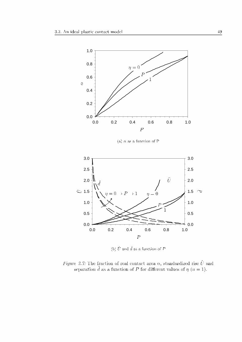
3.2. An ideal plastic contact model 49
0.0 0.2 0.4 0.6 0.8 1.00.0
0.2
0.4
0.6
0.8
1.0
P
�1
P
� = 0
(a) � as a function of P
0.0 0.2 0.4 0.6 0.8 1.00.0
0.5
1.0
1.5
2.0
2.5
3.0
0.0
0.5
1.0
1.5
2.0
2.5
3.0
P
~U
~ U
~d
~ d� = 0! P ! 1
1P
� = 0
(b) ~U and ~d as a function of P
Figure 3.7: The fraction of real contact area �, standardized rise ~U andseparation ~d as a function of P for di�erent values of � (n = 1).
50 Chapter 3: A newly developed contact model
with:
M = �
rm
2(3.58)
and:
N =�p2m
(3.59)
m is an integer and � is the standard deviation of an equivalent Gaussian heightdistribution function. Eq. (3.57) can be standardized, giving:
~��2m(~z) =
exp
�
~M � ~z
2 ~N
!2m2 ~N
m2 ��m2
� ( ~M � ~z)m2�1
(3.60)
with:
~M =
rm
2(3.61)
and:
~N =1p2m
(3.62)
Fig. 3.8 shows scaled �2m-functions for di�erent values of m. An equivalentGaussian distribution function is also shown in Fig. 3.8. As Fig. 3.8 shows, �2m-distribution functions do not include asperities higher than z = m. It also showsthat for larger m-values the �2m-function more closely approaches a Gaussiandistribution.
In Fig. 3.9 � is plotted versus P, applying �2m-distribution functions withm=3, 5, 10 and 20. Calculations were performed for � = P and n = 1. From Fig.3.9 it can be concluded that when a �2m-height distribution function is substitutedin the ideal plastic contact model, � is less than when a Gaussian height distri-bution function is applied. This e�ect can be explained by the fact that the tailof the Gaussian distribution function is larger than that of the �2m-distributionfunction.
Real height distribution functionInstead of substituting mathematical height distribution functions, a real (mea-sured) distribution function can also be substituted. As an example, the realdistribution function shown in Fig. 3.8, with an equivalent Gaussian standarddeviation � = 1:22 �m is substituted in the contact model. In Fig. 3.9 the pre-dicted fraction of real contact area is shown. In chapters 4 and 5 real asperityheight distribution functions will be applied more often.

3.2. An ideal plastic contact model 51
-4 -3 -2 -1 0 1 2 3 40.0
0.1
0.2
0.3
0.4
0.5
0.6
~z
~ �(~ z)
Gauss
m = 3! 5!10! 20
real distributionfunction
Figure 3.8: Standardized scaled �2m-distribution functions for m=3, 5,10 and 20 and the equivalent standardized Gaussian distributionfunction; a real distribution function is also plotted.
0.0 0.2 0.4 0.6 0.8 1.00.0
0.2
0.4
0.6
0.8
1.0
P
�
�2mrealGauss
m = 20! 10! 5! 3
Figure 3.9: The fraction of real contact area � as a function of P for�2m-distribution functions with di�erent values of m, a Gaussianfunction and a real function.
52 Chapter 3: A newly developed contact model
3.2.3 No surface rise
When no rise of the valleys occurs (i.e., U = 0), Wintri = 0 (see eq. (3.30)) andeq. (3.50) can be replaced by:
P = �0 (3.63)
with:
�0 = �0(d; FN(z)) =
Z 1
d
FN (z)�(z)dz �Z 1
d
(z � d)�(z)dzZ 1
d
FN (z)(z � d)�(z)dz
(3.64)
A relation between � and d is given by (eq. (3.44)):
� =
Z 1
d
�(z)dz (3.65)
Substituting eq. (3.52) into eq. (3.64), yields:
�0 =
Z 1
d
(z � d)n�(z)dz �Z 1
d
(z � d)�(z)dzZ 1
d
(z � d)n+1�(z)dz
(3.66)
Eq. (3.63) and eq. (3.65) can be solved simultaneously to obtain � and ~d (d=�)as a function of P and n. Fig. 3.10(a) and Fig. 3.10(b) give, respectively, �and ~d as a function of pnom=H for n=0, n=1, n=2 and n=3. When U = 0, Fig.3.10(a) shows that for n = 0 the relation between � and P is linear and agreeswith the result of Fig. 3.6(a) for n = 0. For low loads the results agree with thosefor � = 0, plotted in Fig. 3.6, because U is small and hardly a�ects the valueof �. However, for higher loads the results for � = 0 become larger than thosefor U = 0, because the value of U a�ects �. Fig. 3.10(b) shows that in contrastto previous results the dimensionless separation becomes negative for high loads.The reason for this phenomenon is that when U = 0, the indenter can be underthe mean plane of the rough surface, causing negative separations. In the case ofa rising surface, the separation is always positive.
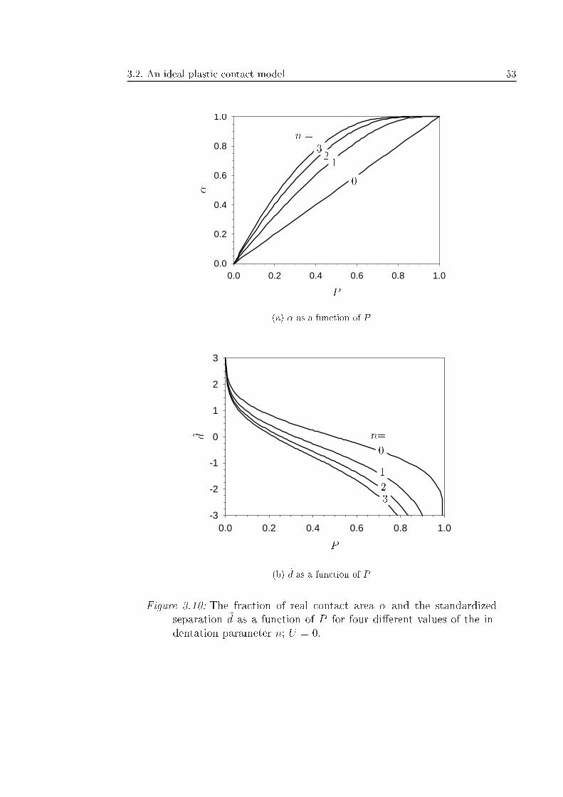
3.2. An ideal plastic contact model 53
0.0 0.2 0.4 0.6 0.8 1.00.0
0.2
0.4
0.6
0.8
1.0
P
�0
12
3n =
(a) � as a function of P
0.0 0.2 0.4 0.6 0.8 1.0-3
-2
-1
0
1
2
3
P
~ d
0
1
23
n=
(b) ~d as a function of P
Figure 3.10: The fraction of real contact area � and the standardizedseparation ~d as a function of P for four di�erent values of the in-dentation parameter n; U = 0.
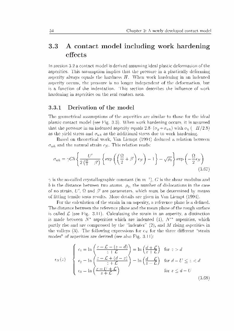
54 Chapter 3: A newly developed contact model
3.3 A contact model including work hardening
e�ects
In section 3.2 a contact model is derived assuming ideal plastic deformation of theasperities. This assumption implies that the pressure in a plastically deformingasperity always equals the hardness H. When work hardening in an indentedasperity occurs, the pressure is no longer independent of the deformation, butis a function of the indentation. This section describes the in uence of workhardening in asperities on the real contact area.
3.3.1 Derivation of the model
The geometrical assumptions of the asperities are similar to those for the idealplastic contact model (see Fig. 3.3). When work hardening occurs, it is assumedthat the pressure in an indented asperity equals 2:8 � (�y+�wh) with �y (=H/2.8)as the yield stress and �wh as the additional stress due to work hardening.
Based on theoretical work, Van Liempt (1994) deduced a relation between�wh and the natural strain �N . This relation reads:
�wh = Gb
(U 0
2�
2+ � 0
� �exp��2+ � 0
��N
�� 1
�+p�0
)exp
��2�N
�(3.67)
is the so-called crystallographic constant (in m�1), G is the shear modulus andb is the distance between two atoms. �0, the number of dislocations in the caseof no strain, U 0, and � 0 are parameters, which must be determined by meansof �tting tensile tests results. More details are given in Van Liempt (1994).
For the calculation of the strain in an asperity, a reference plane is a de�ned.The distance between the reference plane and the mean plane of the rough surfaceis called L (see Fig. 3.11). Calculating the strain in an asperity, a distinctionis made between N� asperities which are indented (1), N�� asperities, whichpartly rise and are compressed by the \indenter" (2), and M rising asperities inthe valleys (3). The following expressions for �N for the three di�erent \strainmodes" of asperities are derived (see also Fig. 3.11):
�N (z) =
8>>>>><>>>>>:�1 = ln
�z + L � (z � d)
z + L�= ln
�d+ Lz + L
�for z > d
�2 = ln
�z + L+ (d� z)
z + L�= ln
�d+ Lz + L
�for d� U � z < d
�3 = ln�z + U + Lz + L
�for z � d� U
(3.68)
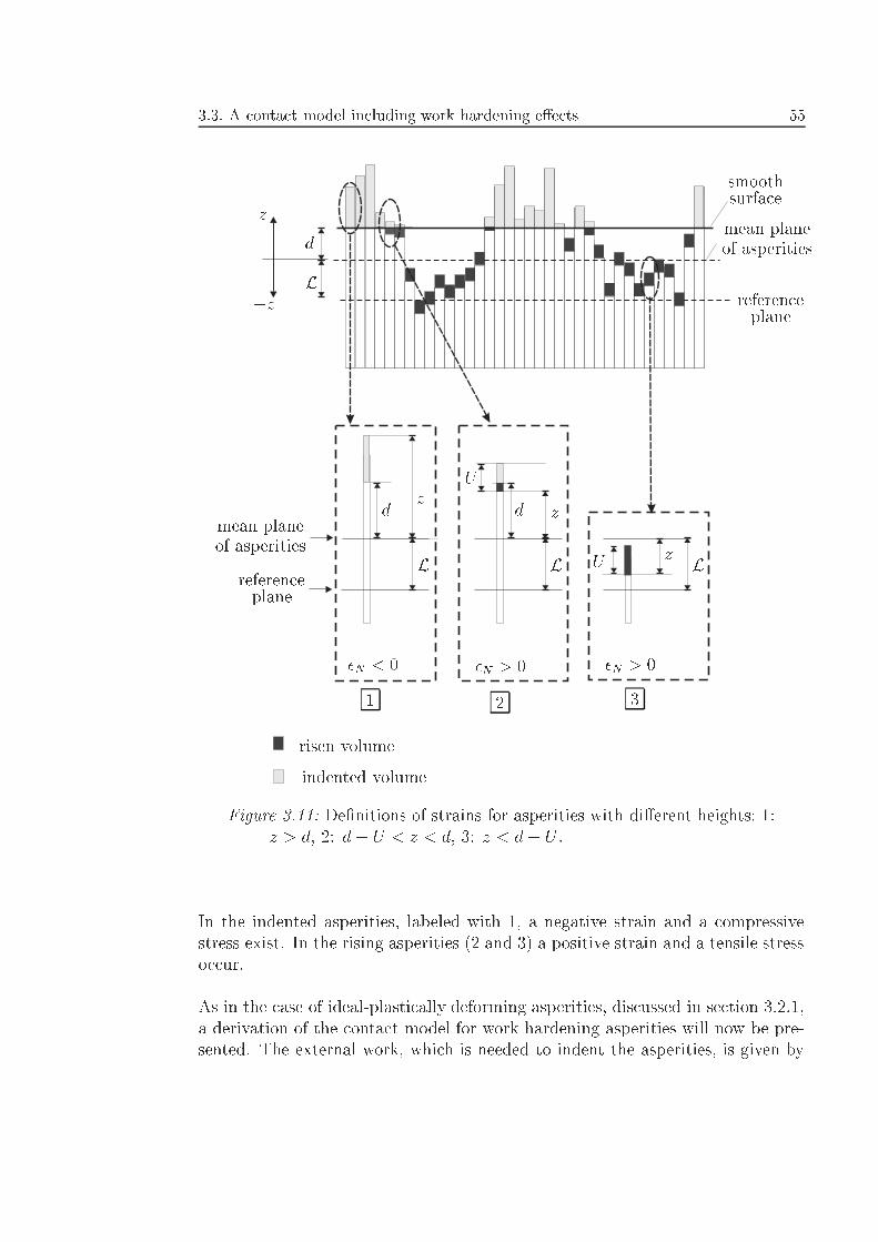
3.3. A contact model including work hardening e�ects 55
mean planeof asperities
smoothsurface
referenceplane
indented volume
risen volume
d
d
d
z
zz
L
LLL U
U
z
�z
mean planeof asperities
referenceplane
�N < 0 �N > 0 �N > 0
1 2 3
Figure 3.11: De�nitions of strains for asperities with di�erent heights; 1:z > d, 2: d� U < z < d, 3: z < d� U .
In the indented asperities, labeled with 1, a negative strain and a compressivestress exist. In the rising asperities (2 and 3) a positive strain and a tensile stressoccur.
As in the case of ideal-plastically deforming asperities, discussed in section 3.2.1,a derivation of the contact model for work hardening asperities will now be pre-sented. The external work, which is needed to indent the asperities, is given by
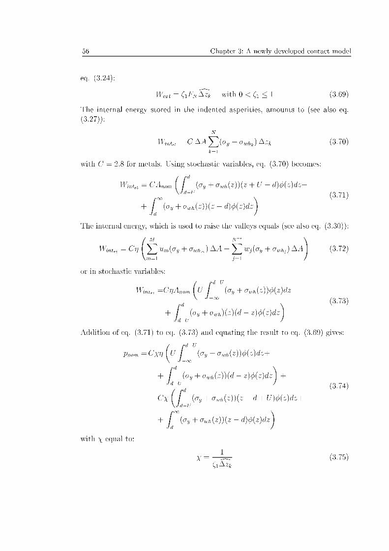
56 Chapter 3: A newly developed contact model
eq. (3.24):
Wext = �1FNd�zk with 0 < �1 � 1 (3.69)
The internal energy stored in the indented asperities, amounts to (see also eq.(3.27)):
Wintst = C�ANXk=1
(�y + �whk)�zk (3.70)
with C = 2:8 for metals. Using stochastic variables, eq. (3.70) becomes:
Wintst = CAnom
�Z d
d�U
(�y + �wh(z))(z + U � d)�(z)dz+
+
Z 1
d
(�y + �wh(z))(z � d)�(z)dz
� (3.71)
The internal energy, which is used to raise the valleys equals (see also eq. (3.30)):
Wintri = C�
MXm=1
um(�y + �whm)�A +N��Xj=1
wj(�y + �whj )�A
!(3.72)
or in stochastic variables:
Wintri =C�Anom
�U
Z d�U
�1
(�y + �wh(z))�(z)dz
+
Z d
d�U
(�y + �wh)(z)(d� z)�(z)dz
� (3.73)
Addition of eq. (3.71) to eq. (3.73) and equating the result to eq. (3.69) gives:
pnom =C��
�U
Z d�U
�1
(�y + �wh(z))�(z)dz+
+
Z d
d�U
(�y + �wh(z))(d� z)�(z)dz
�+
+ C�
�Z d
d�U
(�y + �wh(z))(z � d+ U)�(z)dz+
+
Z 1
d
(�y + �wh(z))(z � d)�(z)dz
�(3.74)
with � equal to:
� =1
�1d�zk (3.75)
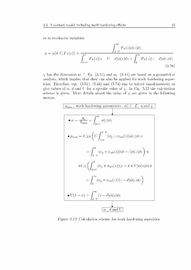
3.3. A contact model including work hardening e�ects 57
or in stochastic variables:
� = �(d; U; FN(z)) =
Z 1
d�U
FN(z)�(z)dzZ d
d�U
FN (z)(z + U � d)�(z)dz +
Z 1
d
FN(z)(z � d)�(z)dz
(3.76)
� has the dimension m�1. Eq. (3.51) and eq. (3.44) are based on a geometricalanalysis, which implies that they can also be applied for work hardening asper-ities. Therefore, eqs. (3.51), (3.44) and (3.74) can be solved simultaneously togive values of �, d and U for a speci�c value of �. In Fig. 3.12 the calculationscheme is given. More details about the value of � are given in the followingsection.
pnom ; work hardening parameters ; �(z) ; L ; � and �
� � = ArAnom
=
Z 1
d�U
�(z)dz
� pnom = C��
�U
Z d�U
�1
(�y + �wh(z))�(z)dz+
+
Z d
d�U
(�y + �wh(z))(d� z)�(z)dz
�+
+C�
�Z d
d�U
(�y + �wh(z))(z � d+ U)�(z)dz+
+
Z 1
d
(�y + �wh(z))(z � d)�(z)dz
�
� U(1� �) =
Z 1
d�U
(z � d)�(z)dz
� ; d and U
Figure 3.12: Calculation scheme for work hardening asperities.
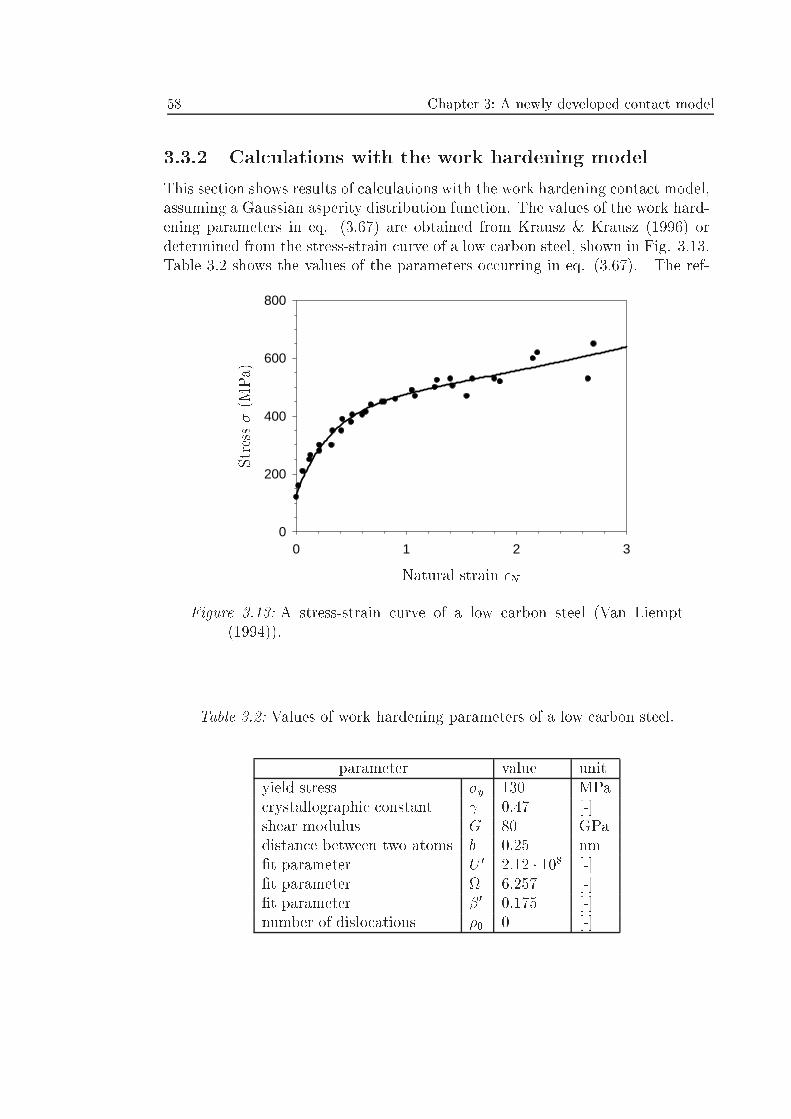
58 Chapter 3: A newly developed contact model
3.3.2 Calculations with the work hardening model
This section shows results of calculations with the work hardening contact model,assuming a Gaussian asperity distribution function. The values of the work hard-ening parameters in eq. (3.67) are obtained from Krausz & Krausz (1996) ordetermined from the stress-strain curve of a low carbon steel, shown in Fig. 3.13.Table 3.2 shows the values of the parameters occurring in eq. (3.67). The ref-
0 1 2 30
200
400
600
800
Natural strain �N
St re ss�( MPa)
Figure 3.13: A stress-strain curve of a low carbon steel (Van Liempt(1994)).
Table 3.2: Values of work hardening parameters of a low carbon steel.
parameter value unityield stress �y 130 MPacrystallographic constant 0.47 [-]shear modulus G 80 GPadistance between two atoms b 0.25 nm�t parameter U 0 2:12 � 108 [-]�t parameter 6.257 [-]�t parameter � 0 0.175 [-]number of dislocations �0 0 [-]
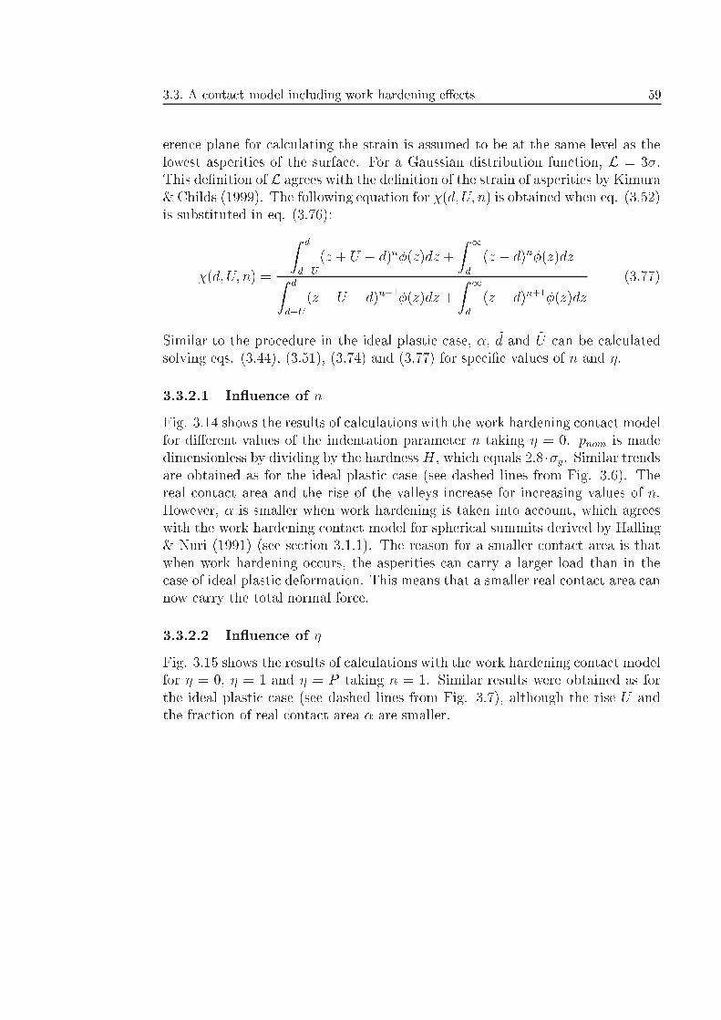
3.3. A contact model including work hardening e�ects 59
erence plane for calculating the strain is assumed to be at the same level as thelowest asperities of the surface. For a Gaussian distribution function, L = 3�.This de�nition of L agrees with the de�nition of the strain of asperities by Kimura& Childs (1999). The following equation for �(d; U; n) is obtained when eq. (3.52)is substituted in eq. (3.76):
�(d; U; n) =
Z d
d�U
(z + U � d)n�(z)dz +
Z 1
d
(z � d)n�(z)dzZ d
d�U
(z + U � d)n+1�(z)dz +
Z 1
d
(z � d)n+1�(z)dz
(3.77)
Similar to the procedure in the ideal plastic case, �, ~d and ~U can be calculatedsolving eqs. (3.44), (3.51), (3.74) and (3.77) for speci�c values of n and �.
3.3.2.1 In uence of n
Fig. 3.14 shows the results of calculations with the work hardening contact modelfor di�erent values of the indentation parameter n taking � = 0. pnom is madedimensionless by dividing by the hardness H, which equals 2:8��y. Similar trendsare obtained as for the ideal plastic case (see dashed lines from Fig. 3.6). Thereal contact area and the rise of the valleys increase for increasing values of n.However, � is smaller when work hardening is taken into account, which agreeswith the work hardening contact model for spherical summits derived by Halling& Nuri (1991) (see section 3.1.1). The reason for a smaller contact area is thatwhen work hardening occurs, the asperities can carry a larger load than in thecase of ideal plastic deformation. This means that a smaller real contact area cannow carry the total normal force.
3.3.2.2 In uence of �
Fig. 3.15 shows the results of calculations with the work hardening contact modelfor � = 0, � = 1 and � = P taking n = 1. Similar results were obtained as forthe ideal plastic case (see dashed lines from Fig. 3.7), although the rise U andthe fraction of real contact area � are smaller.
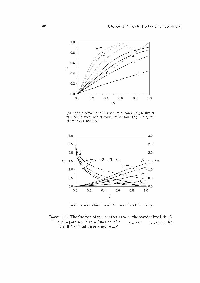
60 Chapter 3: A newly developed contact model
0.0 0.2 0.4 0.6 0.8 1.00.0
0.2
0.4
0.6
0.8
1.0
P
�0 0
1 1
2 23 3
n = n =
(a) � as a function of P in case of work hardening; results ofthe ideal plastic contact model, taken from Fig. 3.6(a) areshown by dashed lines
0.0 0.2 0.4 0.6 0.8 1.00.0
0.5
1.0
1.5
2.0
2.5
3.0
0.0
0.5
1.0
1.5
2.0
2.5
3.0
P
0
123
~U~ U
~d
~ dn =
n = 3! 2! 1! 0
(b) ~U and ~d as a function of P in case of work hardening
Figure 3.14: The fraction of real contact area �, the standardized rise ~Uand separation ~d as a function of P = pnom=H = pnom=2:8�y forfour di�erent values of n and � = 0.
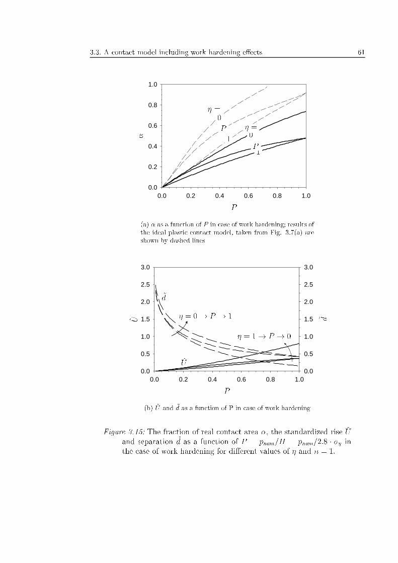
3.3. A contact model including work hardening e�ects 61
0.0 0.2 0.4 0.6 0.8 1.00.0
0.2
0.4
0.6
0.8
1.0
P
� 1
1
P
P
0
0
� =
� =
(a) � as a function of P in case of work hardening; results ofthe ideal plastic contact model, taken from Fig. 3.7(a) areshown by dashed lines
0.0 0.2 0.4 0.6 0.8 1.00.0
0.5
1.0
1.5
2.0
2.5
3.0
0.0
0.5
1.0
1.5
2.0
2.5
3.0
P
~U
~ U
~d
~ d� = 0! P ! 1
� = 1! P ! 0
(b) ~U and ~d as a function of P in case of work hardening
Figure 3.15: The fraction of real contact area �, the standardized rise ~Uand separation ~d as a function of P = pnom=H = pnom=2:8 � �y inthe case of work hardening for di�erent values of � and n = 1.
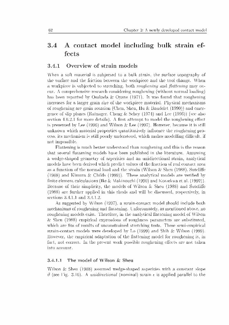
62 Chapter 3: A newly developed contact model
3.4 A contact model including bulk strain ef-
fects
3.4.1 Overview of strain models
When a soft material is subjected to a bulk strain, the surface topography ofthe surface and the friction between the workpiece and the tool change. Whena workpiece is subjected to stretching, both roughening and attening may oc-cur. A comprehensive research considering roughening (without normal loading)has been reported by Osakada & Oyane (1971). It was found that rougheningincreases for a larger grain size of the workpiece material. Physical mechanismsof roughening are grain rotation (Chen, Shen, Hu & Baudelet (1990)) and emer-gence of slip planes (Ratnager, Cheng & Schey (1974) and Lee (1996)) (see alsosection 4.6.2.1 for more details). A �rst attempt to model the roughening e�ectis presented by Lee (1996) and Wilson & Lee (1997). However, because it is stillunknown which material properties quantitatively in uence the roughening pro-cess, its mechanism is still poorly understood, which makes modelling diÆcult, ifnot impossible.
Flattening is much better understood than roughening and this is the reasonthat several attening models have been published in the literature. Assuminga wedge-shaped geometry of asperities and an unidirectional strain, analyticalmodels have been derived which predict values of the fraction of real contact areaas a function of the normal load and the strain (Wilson & Sheu (1988), Sutcli�e(1988) and Kimura & Childs (1999)). These analytical models are veri�ed by�nite element calculations (Ike & Makinouchi (1990) and Korzekwa et al. (1992)).Because of their simplicity, the models of Wilson & Sheu (1988) and Sutcli�e(1988) are further applied in this thesis and will be discussed, respectively, insections 3.4.1.1 and 3.4.1.2.
As suggested by Wilson (1997), a strain-contact model should include bothmechanisms of roughening and attening. Unfortunately, as mentioned above, noroughening models exist. Therefore, in the analytical attening model of Wilson& Sheu (1988) empirical expressions of roughness parameters are substituted,which are �ts of results of unconstrained stretching tests. These semi-empiricalstrain-contact models were developed by Lo (1999) and Shih & Wilson (1999).However, the empirical adaptation of the attening model for roughening is, infact, not correct. In the present work possible roughening e�ects are not takeninto account.
3.4.1.1 The model of Wilson & Sheu
Wilson & Sheu (1988) assumed wedge-shaped asperities with a constant slope# (see Fig. 3.16). A unidirectional (nominal) strain � is applied parallel to the
3.4. A contact model including bulk strain e�ects 63
# a
`
FN
x
y
z
Figure 3.16: The wedge-shaped geometry of asperities assumed by Wilson& Sheu and Sutcli�e.
orientation of the asperities (i.e., the z-direction). The length of the asperities inthe z-direction is much larger than the width of the asperities. Therefore, a planestress situation may be assumed in the asperities because the stress in z-directioncan be neglected. A plane strain situation occurs in the bulk (�x = 0). Wilson& Sheu (1988) de�ned an indentation speed of the asperities va and an upwardspeed vb of the valleys due to stretching. Performing a geometric analysis, Wilson& Sheu (1988) derived the following di�erential equation for the fraction of realcontact area of one asperity � as a function of the nominal strain �3:
d�
d�=
1
E tan#(3.78)
� is de�ned as:
� =a
`(3.79)
with a as the half width of an asperity and ` as the half asperity spacing (seeFig. 3.16). E, the non-dimensional strain rate, is de�ned as:
E =_�z`
va + vb(3.80)
with _�z as the strain rate in z-direction. Because equally shaped asperities and aconstant asperity spacing are assumed, the fraction of contact area of one asperity� equals the total fraction of contact area �. Wilson & Sheu (1988) de�ned anon-dimensional e�ective hardness Heff as:
Heff =prk
(3.81)
with pr as the real pressure in an asperity and k as the shear strength of thesurface material (k = H=3
p3). Applying an upper bound analysis, a semi-
empirical expression for Heff as a function of E is obtained:
Heff =2
f1(�)E + f2(�)(3.82)
3Wilson & Sheu (1988) assumed small values of # in which case tan# � #
64 Chapter 3: A newly developed contact model
with f1(�) and f2(�) functions of � de�ned as:
f1(�) = 0:515 + 0:345�� 0:86�2 (3.83)
and:
f2(�) =1
2:571� �� � ln(1� �)(3.84)
Because prAr = pnomAnom and using eq. (3.81), the e�ective hardness Heff maybe written as:
Heff =pnom�k
(3.85)
Substituting eq. (3.85) into eq. (3.82), an expression for E is obtained, which,when substituted into eq. (3.78), gives:
d�
d�=
1
tan#
pnomk f1(�)
2�� pnomk f2(�)
(3.86)
The application of an upper bound theory means that the e�ective hardness isoverestimated and the real contact area is underestimated. Eq. (3.82) can beused to plotHeff against E for a certain value of �. Fig. 3.17 shows the results for� = 0:1, � = 0:5 and � = 0:7 as the solid lines. The most important conclusionsare that the e�ective hardness decreases with increasing E and that Heff ! 0when E !1.
3.4.1.2 The model of Sutcli�e
As in the model of Wilson & Sheu (1988), wedge-shaped asperities were assumedby Sutcli�e (1988) (see Fig. 3.16). However, a unidirectional strain perpendicularto the orientation of the asperities is assumed (i.e. the x-direction). Unlike thesituation considered by Wilson & Sheu (1988), the asperities are in a plane strainmode (�z = 0). Therefore, a slipline analysis may be performed assuming an idealplastic material. Sutcli�e introduced a dimensionless parameter, the so-called fanangle �, which reads:
� =pnom4k
1� �
�=Heff
4(1� �) (3.87)
with, because of the geometrical conditions, 0 � � � �=2. Using the sliplinetheory, Sutcli�e was able to calculate the parameter Wde�ned as:
W =va + vb` _�x
(3.88)
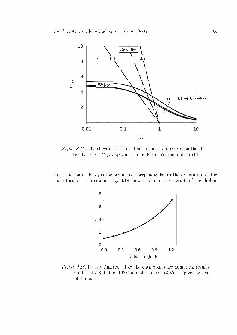
3.4. A contact model including bulk strain e�ects 65
0.01 0.1 1 10
2
4
6
8
10
E
Heff
Wilson
Sutcli�e
0.1 0.5 0.7
� = 0:1! 0:5! 0:7
� =
Figure 3.17: The e�ect of the non-dimensional strain rate E on the e�ec-tive hardness Heff applying the models of Wilson and Sutcli�e.
as a function of �. _�x is the strain rate perpendicular to the orientation of theasperities, i.e. x-direction. Fig. 3.18 shows the numerical results of the slipline
0.0 0.3 0.6 0.9 1.20
2
4
6
8
The fan angle �
W
Figure 3.18: W as a function of �; the data points are numerical resultsobtained by Sutcli�e (1988) and the �t (eq. (3.89)) is given by thesolid line.
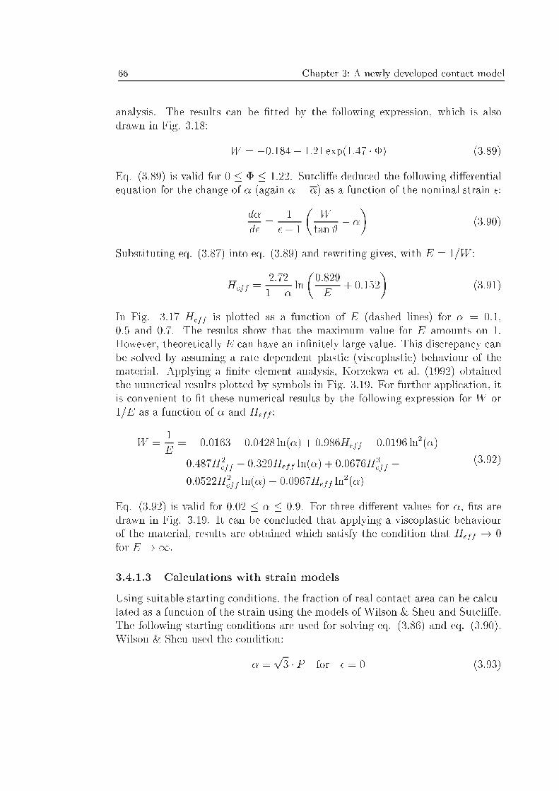
66 Chapter 3: A newly developed contact model
analysis. The results can be �tted by the following expression, which is alsodrawn in Fig. 3.18:
W = �0:184 + 1:21 exp(1:47 � �) (3.89)
Eq. (3.89) is valid for 0 � � � 1:22. Sutcli�e deduced the following di�erentialequation for the change of � (again � = �) as a function of the nominal strain �:
d�
d�=
1
�+ 1
�W
tan#� �
�(3.90)
Substituting eq. (3.87) into eq. (3.89) and rewriting gives, with E = 1=W :
Heff =2:72
1� �ln
�0:829
E+ 0:152
�(3.91)
In Fig. 3.17 Heff is plotted as a function of E (dashed lines) for � = 0:1,0.5 and 0.7. The results show that the maximum value for E amounts on 1.However, theoretically E can have an in�nitely large value. This discrepancy canbe solved by assuming a rate dependent plastic (viscoplastic) behaviour of thematerial. Applying a �nite element analysis, Korzekwa et al. (1992) obtainedthe numerical results plotted by symbols in Fig. 3.19. For further application, itis convenient to �t these numerical results by the following expression for W or1=E as a function of � and Heff :
W =1
E=� 0:0163� 0:0428 ln(�) + 0:986Heff � 0:0196 ln2(�)�0:487H2
eff � 0:329Heff ln(�) + 0:0676H3eff �
0:0522H2eff ln(�)� 0:0967Heff ln
2(�)
(3.92)
Eq. (3.92) is valid for 0:02 � � � 0:9. For three di�erent values for �, �ts aredrawn in Fig. 3.19. It can be concluded that applying a viscoplastic behaviourof the material, results are obtained which satisfy the condition that Heff ! 0for E !1.
3.4.1.3 Calculations with strain models
Using suitable starting conditions, the fraction of real contact area can be calcu-lated as a function of the strain using the models of Wilson & Sheu and Sutcli�e.The following starting conditions are used for solving eq. (3.86) and eq. (3.90).Wilson & Sheu used the condition:
� =p3 � P for � = 0 (3.93)
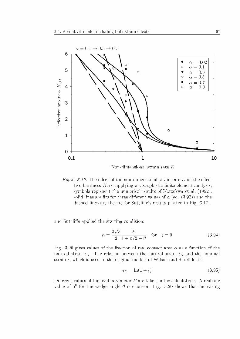
3.4. A contact model including bulk strain e�ects 67
0.1 1 100
1
2
3
4
5
6
Non-dimensional strain rate E
E�ect ivehardnessHeff
� = 0:02� = 0:1� = 0:3� = 0:5� = 0:7� = 0:9
� = 0:1! 0:5! 0:7
Figure 3.19: The e�ect of the non-dimensional strain rate E on the e�ec-tive hardness Heff , applying a viscoplastic �nite element analysis;symbols represent the numerical results of Korzekwa et al. (1992),solid lines are �ts for three di�erent values of � (eq. (3.92)) and thedashed lines are the �ts for Sutcli�e's results plotted in Fig. 3.17.
and Sutcli�e applied the starting condition:
� =3p3
2
P
1 + �=2� #for � = 0 (3.94)
Fig. 3.20 gives values of the fraction of real contact area � as a function of thenatural strain �N . The relation between the natural strain �N and the nominalstrain �, which is used in the original models of Wilson and Sutcli�e, is:
�N = ln(1 + �) (3.95)
Di�erent values of the load parameter P are taken in the calculations. A realisticvalue of 50 for the wedge angle # is choosen. Fig. 3.20 shows that increasing
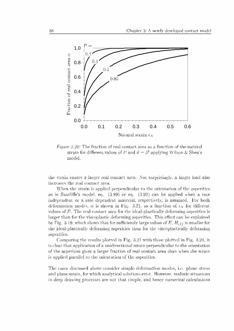
68 Chapter 3: A newly developed contact model
0.0 0.1 0.2 0.3 0.4 0.5 0.60.0
0.2
0.4
0.6
0.8
1.0
Natural strain �N
Fr ac tionofrealc ontacta rea�
P =
0.4
0.2
0.1
0.05
Figure 3.20: The fraction of real contact area as a function of the naturalstrain for di�erent values of P and # = 50 applying Wilson & Sheu'smodel.
the strain causes a larger real contact area. Not surprisingly, a larger load alsoincreases the real contact area.
When the strain is applied perpendicular to the orientation of the asperitiesas in Sutcli�e's model, eq. (3.89) or eq. (3.92) can be applied when a rateindependent or a rate dependent material, respectively, is assumed. For bothdeformation modes, � is shown in Fig. 3.21, as a function of �N for di�erentvalues of P . The real contact area for the ideal-plastically deforming asperities islarger than for the viscoplastic deforming asperities. This e�ect can be explainedby Fig. 3.19, which shows that for suÆciently large values of E, Heff is smaller forthe ideal-plastically deforming asperities than for the viscoplastically deformingasperities.
Comparing the results plotted in Fig. 3.21 with those plotted in Fig. 3.20, itis clear that application of a unidirectional strain perpendicular to the orientationof the asperities gives a larger fraction of real contact area than when the strainis applied parallel to the orientation of the asperities.
The cases discussed above consider simple deformation modes, i.e. plane stressand plane strain, for which analytical solutions exist. However, realistic situationsin deep drawing processes are not that simple, and hence numerical calculations
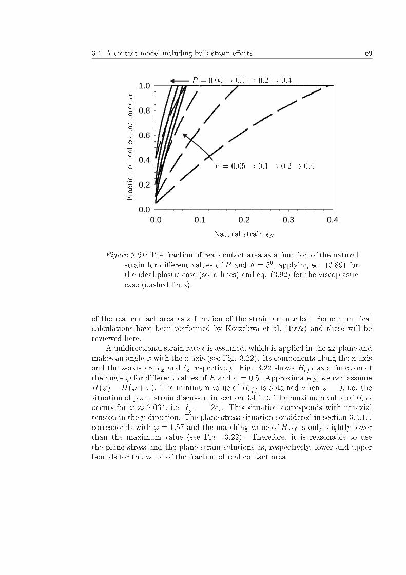
3.4. A contact model including bulk strain e�ects 69
0.0 0.1 0.2 0.3 0.40.0
0.2
0.4
0.6
0.8
1.0
Natural strain �N
Fractionofr ealcontactarea�
P = 0:05! 0:1! 0:2! 0:4
P = 0:05! 0:1! 0:2! 0:4
Figure 3.21: The fraction of real contact area as a function of the naturalstrain for di�erent values of P and # = 50, applying eq. (3.89) forthe ideal plastic case (solid lines) and eq. (3.92) for the viscoplasticcase (dashed lines).
of the real contact area as a function of the strain are needed. Some numericalcalculations have been performed by Korzekwa et al. (1992) and these will bereviewed here.
A unidirectional strain rate _� is assumed, which is applied in the xz-plane andmakes an angle ' with the x-axis (see Fig. 3.22). Its components along the x-axisand the z-axis are _�x and _�z respectively. Fig. 3.22 shows Heff as a function ofthe angle ' for di�erent values of E and � = 0:5. Approximately, we can assumeH(') = H('+ �). The minimum value of Heff is obtained when ' = 0, i.e. thesituation of plane strain discussed in section 3.4.1.2. The maximum value of Heff
occurs for ' � 2:034, i.e. _�y = �2 _�x. This situation corresponds with uniaxialtension in the y-direction. The plane stress situation considered in section 3.4.1.1corresponds with ' = 1:57 and the matching value of Heff is only slightly lowerthan the maximum value (see Fig. 3.22). Therefore, it is reasonable to usethe plane stress and the plane strain solutions as, respectively, lower and upperbounds for the value of the fraction of real contact area.
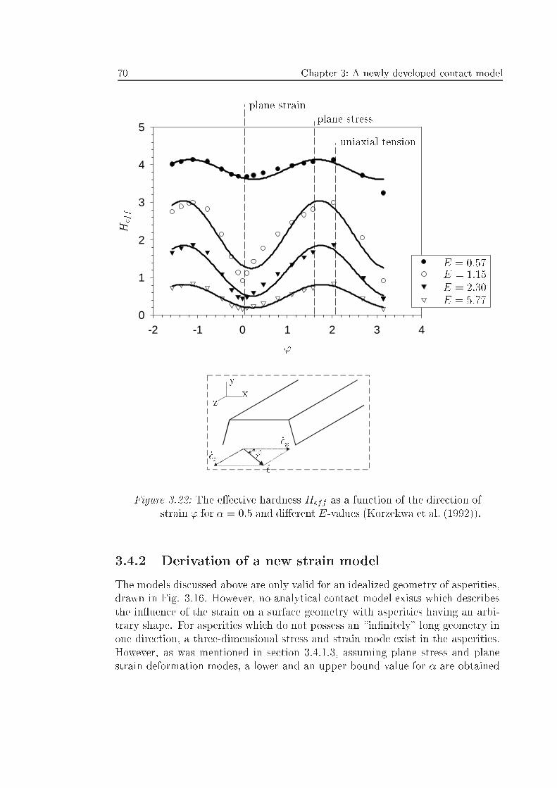
70 Chapter 3: A newly developed contact model
-2 -1 0 1 2 3 40
1
2
3
4
5
'
'
Heff
E = 0:57E = 1:15E = 2:30E = 5:77
_�_�z
_�x
plane strainplane stress
uniaxial tension
zx
y
Figure 3.22: The e�ective hardness Heff as a function of the direction ofstrain ' for � = 0:5 and di�erent E-values (Korzekwa et al. (1992)).
3.4.2 Derivation of a new strain model
The models discussed above are only valid for an idealized geometry of asperities,drawn in Fig. 3.16. However, no analytical contact model exists which describesthe in uence of the strain on a surface geometry with asperities having an arbi-trary shape. For asperities which do not possess an \in�nitely" long geometry inone direction, a three-dimensional stress and strain mode exist in the asperities.However, as was mentioned in section 3.4.1.3, assuming plane stress and planestrain deformation modes, a lower and an upper bound value for � are obtained
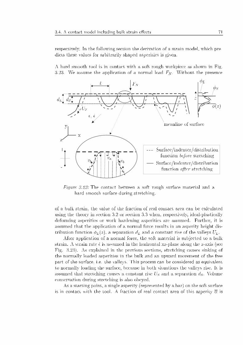
3.4. A contact model including bulk strain e�ects 71
respectively. In the following section the derivation of a strain model, which pre-dicts these values for arbitrarily shaped asperities is given.
A hard smooth tool is in contact with a soft rough workpiece as shown in Fig.3.23. We assume the application of a normal load FN . Without the presence
dSdL z
�(z)
vavb vb
�, _�
US
y
xz
FN`
meanline of surface
Surface/indenter/distributionfunction before stretching
Surface/indenter/distributionfunction after stretching
�L�S
+
-
Figure 3.23: The contact between a soft rough surface material and ahard smooth surface during stretching.
of a bulk strain, the value of the fraction of real contact area can be calculatedusing the theory in section 3.2 or section 3.3 when, respectively, ideal-plasticallydeforming asperities or work hardening asperities are assumed. Further, it isassumed that the application of a normal force results in an asperity height dis-tribution function �L(z), a separation dL and a constant rise of the valleys UL.
After application of a normal force, the soft material is subjected to a bulkstrain. A strain rate _� is assumed in the horizontal xz-plane along the z-axis (seeFig. 3.23). As explained in the previous sections, stretching causes sinking ofthe normally loaded asperities in the bulk and an upward movement of the freepart of the surface, i.e. the valleys. This process can be considered as equivalentto normally loading the surface, because in both situations the valleys rise. It isassumed that stretching causes a constant rise US and a separation dS. Volumeconservation during stretching is also obeyed.
As a starting point, a single asperity (represented by a bar) on the soft surfaceis in contact with the tool. A fraction of real contact area of this asperity � is
72 Chapter 3: A newly developed contact model
de�ned. We are interested in the change in � as a function of the nominal strain�, which for in�nitesimally small changes of � can be written as d�=d�. When tSis the time period of stretching and !S is the attening distance of an asperity4
due to stretching, d�=d� can be written as:
d�
d�=
d�
d!S
d!SdtS
dtSd�
(3.96)
The attening distance of an asperity !S equals (see Fig. 3.23):
!S = dL � dS + US (3.97)
Using eq. (3.97), the �rst term in eq. (3.96) can be written as:
d�
d!S=
d�
d(US � dS)(3.98)
De�ning va as the indentation speed and vb as the upward speed of the freesurface, the second term in eq. (3.96) equals:
d!SdtS
= va + vb (3.99)
Combining eqs. (3.96), (3.98) and (3.99) gives:
d�
d�=va + vb
_�
d�
d(US � dS)(3.100)
A length ` is now introduced, as the mean half asperity spacing (see Fig. 3.23).Using the de�nition of E given by eq. (3.80), eq. (3.100) can be written as:
d�
d�=
`
E
d�
d(US � dS)(3.101)
An expression for the term d�=d(US�dS) in eq. (3.101) is needed. It is assumedthat the fraction of real contact area for one asperity, �, equals the total fractionof contact area �. Therefore, we may di�erentiate the equation:
� =
Z 1
dS�US
�L(z)dz (3.102)
with respect to (US � dS), giving:
d�
d(US � dS)= �L(dS � US) (3.103)
4This de�nition corresponds to the de�nition of the attening speed va + vb by Wilson &Sheu (1988)
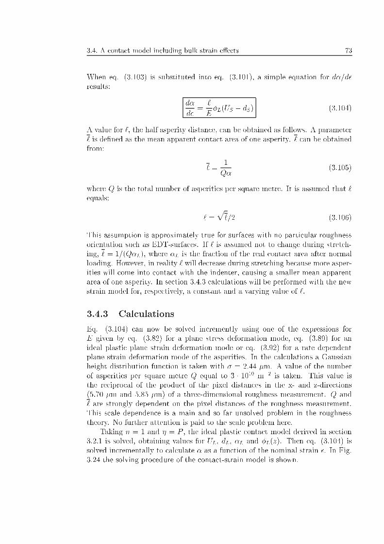
3.4. A contact model including bulk strain e�ects 73
When eq. (3.103) is substituted into eq. (3.101), a simple equation for d�=d�results:
d�
d�=
`
E�L(US � dS) (3.104)
A value for `, the half asperity distance, can be obtained as follows. A parameter` is de�ned as the mean apparent contact area of one asperity. ` can be obtainedfrom:
` =1
Q�(3.105)
where Q is the total number of asperities per square metre. It is assumed that `equals:
` =p`=2 (3.106)
This assumption is approximately true for surfaces with no particular roughnessorientation such as EDT-surfaces. If ` is assumed not to change during stretch-ing, ` = 1=(Q�L), where �L is the fraction of the real contact area after normalloading. However, in reality ` will decrease during stretching because more asper-ities will come into contact with the indenter, causing a smaller mean apparentarea of one asperity. In section 3.4.3 calculations will be performed with the newstrain model for, respectively, a constant and a varying value of `.
3.4.3 Calculations
Eq. (3.104) can now be solved incremently using one of the expressions forE given by eq. (3.82) for a plane stress deformation mode, eq. (3.89) for anideal plastic plane strain deformation mode or eq. (3.92) for a rate dependentplane strain deformation mode of the asperities. In the calculations a Gaussianheight distribution function is taken with � = 2:44 �m. A value of the numberof asperities per square metre Q equal to 3 � 1010 m�2 is taken. This value isthe reciprocal of the product of the pixel distances in the x- and z-directions(5:70 �m and 5:85 �m) of a three-dimensional roughness measurement. Q and` are strongly dependent on the pixel distances of the roughness measurement.This scale dependence is a main and so far unsolved problem in the roughnesstheory. No further attention is paid to the scale problem here.
Taking n = 1 and � = P , the ideal plastic contact model derived in section3.2.1 is solved, obtaining values for UL, dL, �L and �L(z). Then eq. (3.104) issolved incrementally to calculate � as a function of the nominal strain �. In Fig.3.24 the solving procedure of the contact-strain model is shown.
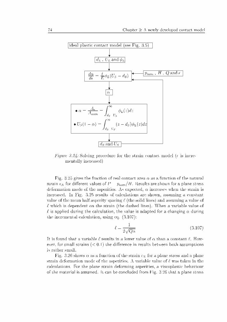
74 Chapter 3: A newly developed contact model
ideal plastic contact model (see Fig. 3.5)
dL ; UL and �L
d�d�
= `E�L(US � dS)
pnom ; H ; Q and �
�
dS and US
� � = ArAnom
=
Z 1
dS�US
�L(z)dz
� US(1� �) =
Z 1
dS�US
(z � dS)�L(z)dz
Figure 3.24: Solving procedure for the strain contact model (� is incre-mentally increased)
Fig. 3.25 gives the fraction of real contact area � as a function of the naturalstrain �N for di�erent values of P = pnom=H. Results are shown for a plane stressdeformation mode of the asperities. As expected, � increases when the strain isincreased. In Fig. 3.25 results of calculations are shown, assuming a constantvalue of the mean half asperity spacing ` (the solid lines) and assuming a value of` which is dependent on the strain (the dashed lines). When a variable value of` is applied during the calculation, the value is adapted for a changing � duringthe incremental calculation, using eq. (3.107):
` =1
2pQ�
(3.107)
It is found that a variable ` results in a lower value of � than a constant `. How-ever, for small strains (< 0:1) the di�erence in results between both assumptionsis rather small.
Fig. 3.26 shows � as a function of the strain �N for a plane stress and a planestrain deformation mode of the asperities. A variable value of ` was taken in thecalculations. For the plane strain deforming asperities, a viscoplastic behaviourof the material is assumed. It can be concluded from Fig. 3.26 that a plane stress
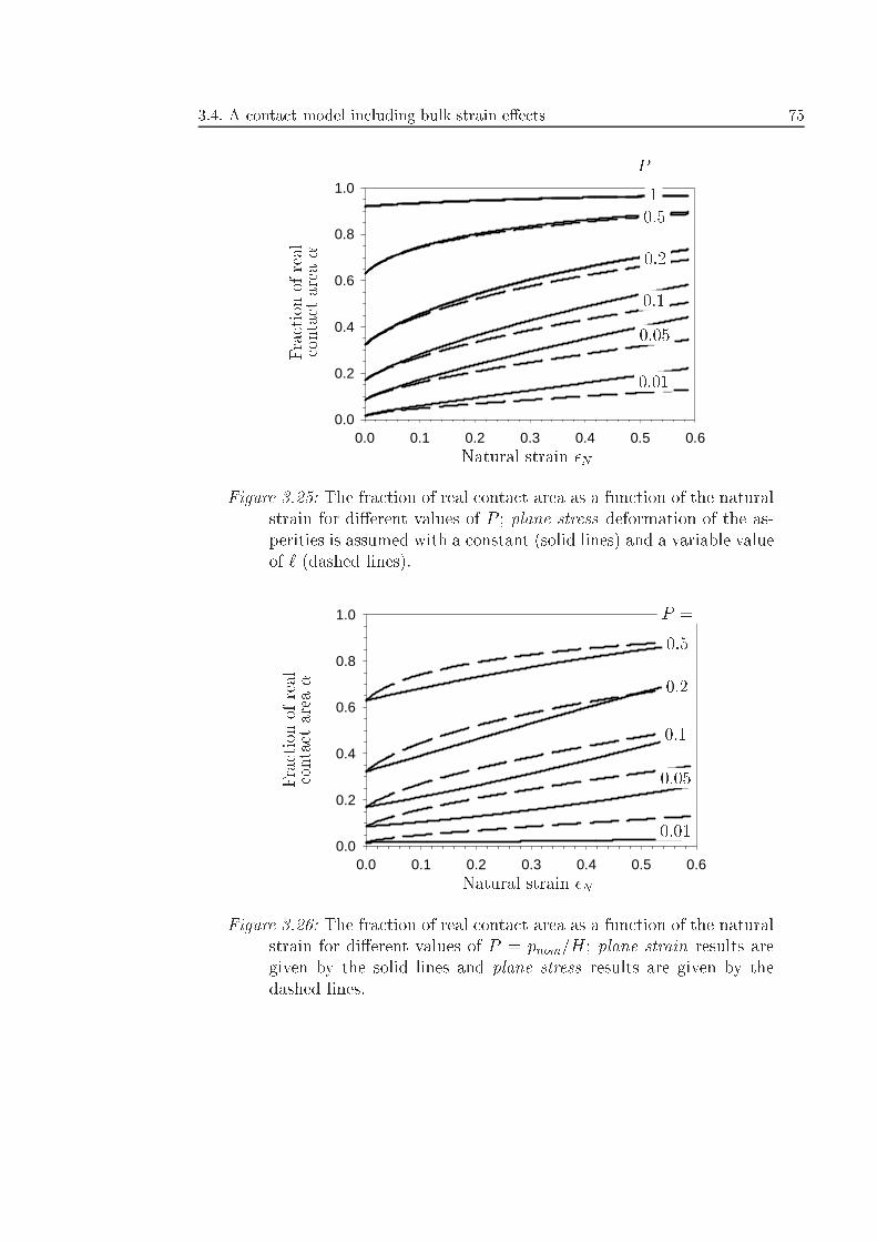
3.4. A contact model including bulk strain e�ects 75
0.0 0.1 0.2 0.3 0.4 0.5 0.60.0
0.2
0.4
0.6
0.8
1.0
Natural strain �N
Frac ti onofreal
c ontactarea�
0:01
0:05
0:1
0:2
0:5
1
P =
Figure 3.25: The fraction of real contact area as a function of the naturalstrain for di�erent values of P ; plane stress deformation of the as-perities is assumed with a constant (solid lines) and a variable valueof ` (dashed lines).
0.0 0.1 0.2 0.3 0.4 0.5 0.60.0
0.2
0.4
0.6
0.8
1.0
Natural strain �N
Fractiono frea l
cont ac tarea�
0:01
0:05
0:1
0:2
0:5
P =
Figure 3.26: The fraction of real contact area as a function of the naturalstrain for di�erent values of P = pnom=H; plane strain results aregiven by the solid lines and plane stress results are given by thedashed lines.
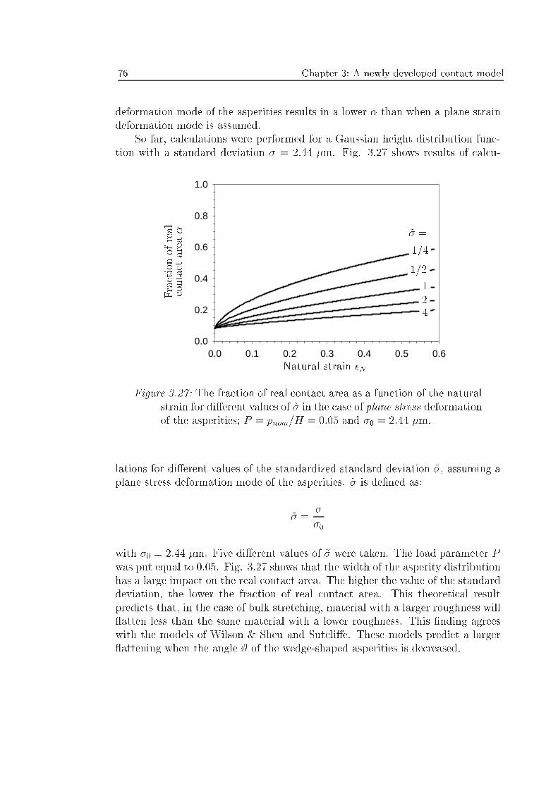
76 Chapter 3: A newly developed contact model
deformation mode of the asperities results in a lower � than when a plane straindeformation mode is assumed.
So far, calculations were performed for a Gaussian height distribution func-tion with a standard deviation � = 2:44 �m. Fig. 3.27 shows results of calcu-
0.0 0.1 0.2 0.3 0.4 0.5 0.60.0
0.2
0.4
0.6
0.8
1.0
Natural strain �N
Fractionofr eal
contac ta re a�
1/4
1/2
124
~� =
Figure 3.27: The fraction of real contact area as a function of the naturalstrain for di�erent values of ~� in the case of plane stress deformationof the asperities; P = pnom=H = 0:05 and �0 = 2:44 �m.
lations for di�erent values of the standardized standard deviation ~�, assuming aplane stress deformation mode of the asperities. ~� is de�ned as:
~� =�
�0
with �0 = 2:44 �m. Five di�erent values of ~� were taken. The load parameter Pwas put equal to 0.05. Fig. 3.27 shows that the width of the asperity distributionhas a large impact on the real contact area. The higher the value of the standarddeviation, the lower the fraction of real contact area. This theoretical resultpredicts that, in the case of bulk stretching, material with a larger roughness will atten less than the same material with a lower roughness. This �nding agreeswith the models of Wilson & Sheu and Sutcli�e. These models predict a larger attening when the angle # of the wedge-shaped asperities is decreased.
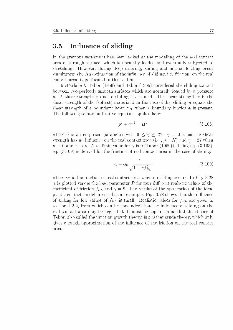
3.5. In uence of sliding 77
3.5 In uence of sliding
In the previous sections it has been looked at the modelling of the real contactarea of a rough surface, which is normally loaded and eventually subjected tostretching. However, during deep drawing, sliding and normal loading occursimultaneously. An estimation of the in uence of sliding, i.e. friction, on the realcontact area, is performed in this section.
McFarlane & Tabor (1950) and Tabor (1959) considered the sliding contactbetween two perfectly smooth surfaces which are normally loaded by a pressurep. A shear strength � due to sliding is assumed. The shear strength � is theshear strength of the (softest) material k in the case of dry sliding or equals theshear strength of a boundary layer �BL when a boundary lubricant is present.The following semi-quantitative equation applies here:
p2 + � 2 = H2 (3.108)
where is an empirical parameter with 0 � � 27. = 0 when the shearstrength has no in uence on the real contact area (i.e., p = H) and = 27 whenp! 0 and � ! k. A realistic value for is 9 (Tabor (1959)). Using eq. (3.108),eq. (3.109) is derived for the fraction of real contact area in the case of sliding:
� = �01p
1� f 2BL(3.109)
where �0 is the fraction of real contact area when no sliding occurs. In Fig. 3.28� is plotted versus the load parameter P for four di�erent realistic values of thecoeÆcient of friction fBL and = 9. The results of the application of the idealplastic contact model are used as an example. Fig. 3.28 shows that the in uenceof sliding for low values of fBL is small. Realistic values for fBL are given insection 2.2.2, from which can be concluded that the in uence of sliding on thereal contact area may be neglected. It must be kept in mind that the theory ofTabor, also called the junction growth theory, is a rather crude theory, which onlygives a rough approximation of the in uence of the friction on the real contactarea.
78 Chapter 3: A newly developed contact model
0.0 0.2 0.4 0.6 0.8 1.00.0
0.2
0.4
0.6
0.8
1.0
Load parameter P
Fr ac ti onofr ea lc ontactarea�
fBL = 0:16! 0:12! 0:08! 0:04! 0
fBL �=�00 1
0.04 1.0070.08 1.030.12 1.070.16 1.14
Figure 3.28: The in uence of sliding on � for di�erent values of fBL with = 9; the curve for fBL = 0 is calculated for an ideal plasticdeforming material; the table lists the relative growth of the realcontact area in the case of sliding.
3.6 Conclusions and summmary
In this chapter a new contact model is presented, which shows several improve-ments compared to the classical contact models discussed in section 3.1. Themain additional features of the new contact model are:
� The contact model describes the deformations of asperities during applica-tion of a normal load, which makes it useful for low and high normal loads.The contact models discussed in section 3.1.1 consider only deformationsof summits, which limits the application of these models below a certainnormal load. The model can be used to calculate the real contact area forreal asperity height distribution functions.
� It is assumed that when a normal load is applied, the parts of the surface,which do not carry the normal load (i.e. the valleys) rise. In the derivationof the ideal plastic contact model in section 3.2.1, it is assumed that this riseU is constant. However, according to the results of experiments discussed in
3.6. Conclusions and summmary 79
chapter 4 and the contact model of Chang et al. (1987) (see section 3.1.1),shallow valleys rise more than deep valleys. A similar derivation of the idealplastic contact model can be performed when an arbitrary function for therise u(z) is substituted into eq. (3.32) and eq. (3.35).
� In the contact model the in uence of asperity persistence is taken intoaccount by introducing the persistence parameter � with 0 � � � 1. Thelarger the value of �, the larger the in uence of asperity persistence andthe smaller the real contact area. � is not necessarily constant during anincrease of the load parameter P (= pnom=H), but can vary when P isincreased. In this chapter results of calculations are presented for � = P .
� Apart from an ideal-plastically deforming material, also the in uence ofwork hardening on the real contact area has been taken into account. Whenwork hardening occurs, a lower real contact area is predicted than for anideal-plastically deforming material. When work hardening occurs, the realpressure in an asperity is larger than the hardness, causing a lower realcontact area.
� The application of a bulk deformation implies an increase of the real contactarea. The amount of attening depends on the deformation mode in theasperities. Plane strain deformation gives a larger real contact area thanplane stress deformation (Fig. 3.25 and Fig. 3.26). Also the height dis-tribution function in uences the amount of attening, predicting a largerreal contact area when the standard deviation of the distribution functionis decreased (Fig. 3.27).
The attening process, predicted by the ideal plastic contact model, depends onthe applied nominal pressure, the hardness of the material and the asperity heightdistribution function.
When work hardening is assumed, the real contact area is not only in uencedby the nominal pressure and the height distribution function, but also by the workhardening parameters as described in the relation of Van Liempt (eq. (3.67)).An additional diÆculty of introducing work hardening is the question of how todetermine the distance L between the reference plane and the mean plane of theasperities. This distance can be regarded as a measure for how much indentingan asperity a�ects the stress in the material. The larger the value of L, the largerthe in uence of an applied normal force on the subsurface material. Therefore,L may not be a constant, as is assumed in the calculations in section 3.3.2, butcan increase when a larger load is applied.
Analytical calculations of the in uence of the bulk strain on the real contactarea are only possible when a plane strain or a plane stress deformation mode inthe asperities is assumed. In these calculations it is assumed that the normal and
80 Chapter 3: A newly developed contact model
the tensile load are simultaneously applied. Application of a bulk strain causesa decrease of the \e�ective hardness", which results in attening of the surface.When a surface is assumed to deform in a plane stress mode, the attening islarger than for a viscoplastic material, which deforms in a plane strain situation.Because in realistic situations asperities deform in a more complicated mode,the results for the plane strain and the plane stress mode can be considered as,respectively, lower and upper bound values (see section 3.4.1.3).
In this chapter no attention has been paid to elastically deforming asperities.In sheet metal forming processes the e�ect of elastic deforming asperities on thefriction process is usually neglected, in accordance with the high value of theplasticity index (eq. (3.12)).
In deep drawing, sliding and, consequently, friction occur between the work-piece and the tool. In section 3.5 the in uence of friction on the real contact areais investigated by application of the junction growth theory proposed by Tabor(1959). It is shown that the in uence of the shear strength on the real contactarea may be neglected, because the friction for BL is low (see section 2.2.2).
In chapter 4 a number of experiments will be presented carried out in orderto verify the theoretical work discussed here.
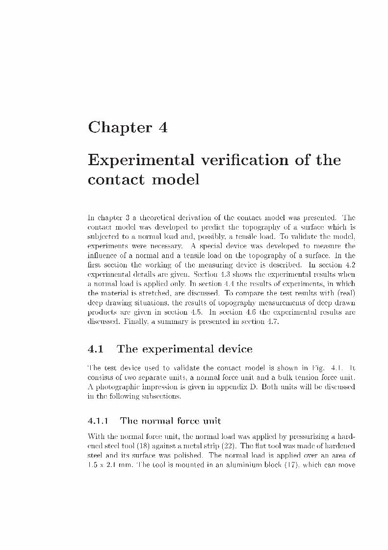
Chapter 4
Experimental veri�cation of thecontact model
In chapter 3 a theoretical derivation of the contact model was presented. Thecontact model was developed to predict the topography of a surface which issubjected to a normal load and, possibly, a tensile load. To validate the model,experiments were necessary. A special device was developed to measure thein uence of a normal and a tensile load on the topography of a surface. In the�rst section the working of the measuring device is described. In section 4.2experimental details are given. Section 4.3 shows the experimental results whena normal load is applied only. In section 4.4 the results of experiments, in whichthe material is stretched, are discussed. To compare the test results with (real)deep drawing situations, the results of topography measurements of deep drawnproducts are given in section 4.5. In section 4.6 the experimental results arediscussed. Finally, a summary is presented in section 4.7.
4.1 The experimental device
The test device used to validate the contact model is shown in Fig. 4.1. Itconsists of two separate units, a normal force unit and a bulk tension force unit.A photographic impression is given in appendix D. Both units will be discussedin the following subsections.
4.1.1 The normal force unit
With the normal force unit, the normal load was applied by pressurizing a hard-ened steel tool (18) against a metal strip (22). The at tool was made of hardenedsteel and its surface was polished. The normal load is applied over an area of1.5 x 2.1 mm. The tool is mounted in an aluminium block (17), which can move
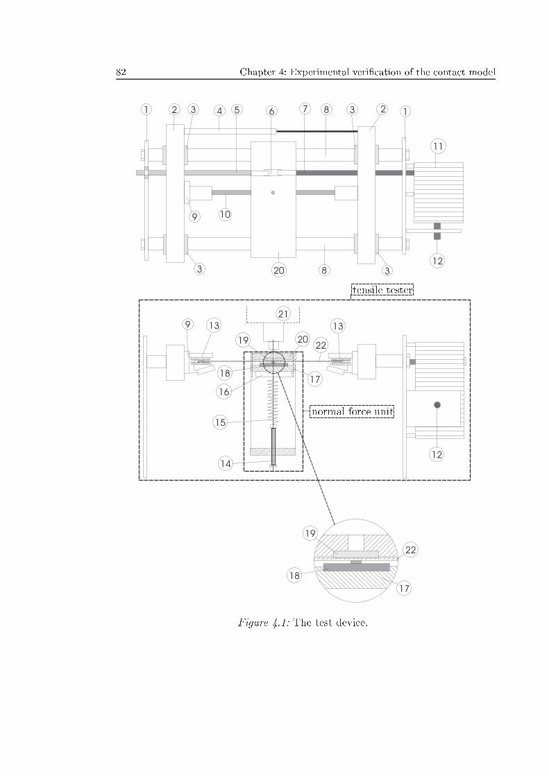
82 Chapter 4: Experimental veri�cation of the contact model
1 12 2
11
12
13
14
15
16
17
17
18
18
19
19
2022
22
20
21
12
109
9
8
8
4 5 6 73
3 3
3
13
normal force unit
tensile tester
Figure 4.1: The test device.
4.1. The experimental device 83
freely along vertical guides. The normal force is applied by means of tighteninga sti� spring (15) with a screw (14). A force transducer (16) enables the mea-surement of the normal load. The whole construction is mounted in a frame (20)clamped onto the translation guides (8) of a tensile tester unit. In the upper partof the normal force unit a sapphire disk (19) is mounted, which enables opticalmeasurement of the roughness of the surface of the strip. A three-dimensionaloptical roughness measurement apparatus (21) is used described in Lubbinge(1994). The magni�cation of the objective used for the measurements amountedto 2.5. Using this magni�cation, the dimensions of the measurement area were1.33 mm x 1.73 mm. The height resolution was less than 1 nm and the lateralresolution was 5.70 x 5.85 �m.
4.1.2 The bulk tension force unit
The second unit of the device shown in Fig. 4.1 is the bulk tension force unit.This consists of a �xed frame (1) in which two thick sti� guides (8) are mounted.Along brass slide rings (3), mounted on these guides, two sti� aluminium blocks(2) can be moved laterally. The blocks are driven by two spindles (5 and 7) withscrew threads in di�erent directions. The spindles are connected to each otherin the upper part of the normal force unit (20). When the spindles (5 and 7)are driven, the blocks move towards or from each other. Between these blocksa metal strip (10) is clamped by means of \self-clamping" units (13) attachedto the blocks. In this way a bulk tension force is applied to the strip. Thespindles (5 and 7) are driven by a turning axis (12) with an electric motor, whichis connected to the spindles by a transmission box (11). The tension force ismeasured with a force transducer (9) installed in line with the clamping unitsto avoid force moments. A displacement transducer (4) is used to measure theelongation �l of the strip. With l0 as the initial length of the strip, the naturalstrain �N is de�ned as:
�N = ln
�l0 +�l
l0
�(4.1)
With the experimental device described above, it is possible to measure thechange of the roughness and the real contact area as a function of the strainduring in situ application of a normal load. During stretching, sliding in thecentre of the strip between the sapphire disk and the strip material is practicallyzero.
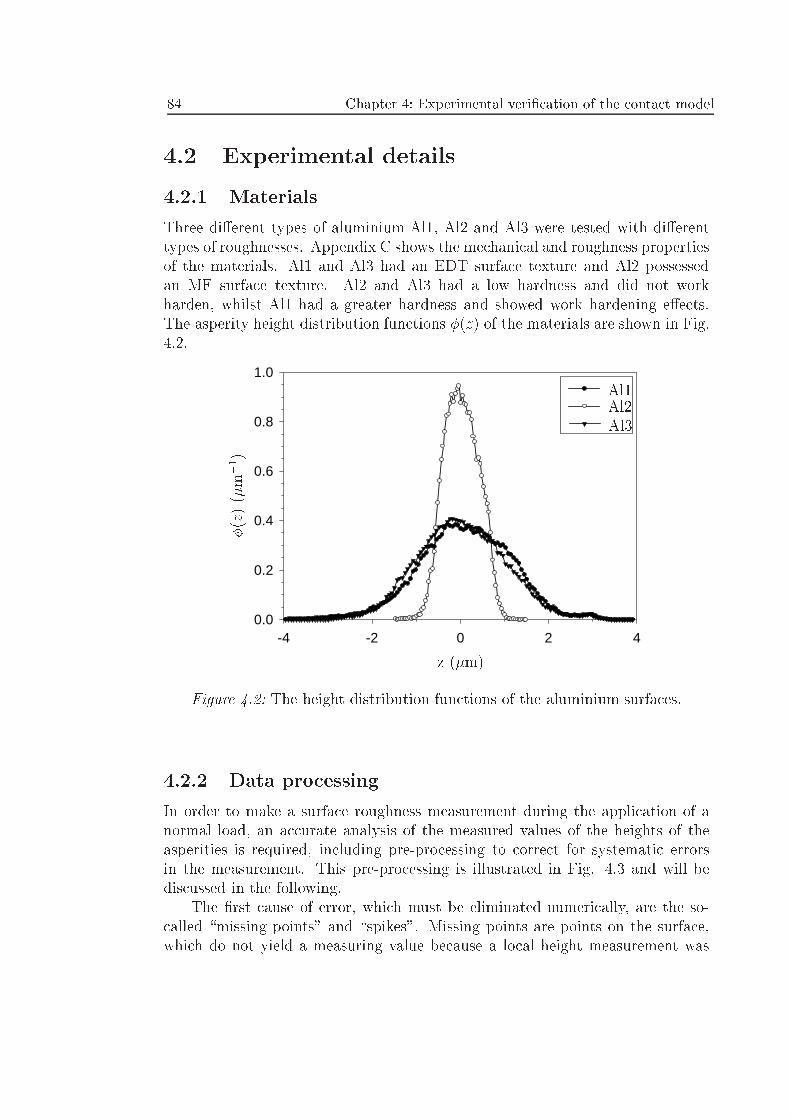
84 Chapter 4: Experimental veri�cation of the contact model
4.2 Experimental details
4.2.1 Materials
Three di�erent types of aluminium Al1, Al2 and Al3 were tested with di�erenttypes of roughnesses. Appendix C shows the mechanical and roughness propertiesof the materials. Al1 and Al3 had an EDT surface texture and Al2 possessedan MF surface texture. Al2 and Al3 had a low hardness and did not workharden, whilst Al1 had a greater hardness and showed work hardening e�ects.The asperity height distribution functions �(z) of the materials are shown in Fig.4.2.
-4 -2 0 2 40.0
0.2
0.4
0.6
0.8
1.0
z (�m)
�( z)(�m�1)
Al1Al2Al3
Figure 4.2: The height distribution functions of the aluminium surfaces.
4.2.2 Data processing
In order to make a surface roughness measurement during the application of anormal load, an accurate analysis of the measured values of the heights of theasperities is required, including pre-processing to correct for systematic errorsin the measurement. This pre-processing is illustrated in Fig. 4.3 and will bediscussed in the following.
The �rst cause of error, which must be eliminated numerically, are the so-called \missing points" and \spikes". Missing points are points on the surface,which do not yield a measuring value because a local height measurement was
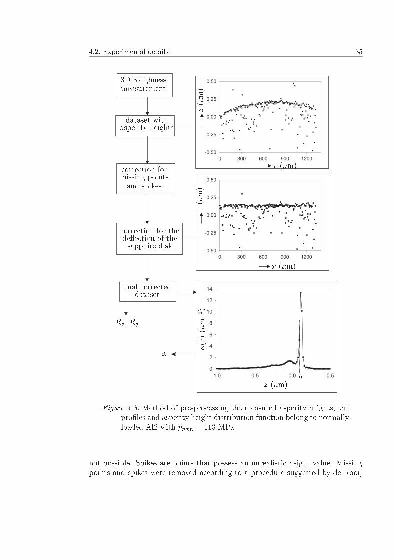
4.2. Experimental details 85
-1.0 -0.5 0.0 0.5
0
2
4
6
8
10
12
14
0 300 600 900 1200
-0.50
-0.25
0.00
0.25
0.50
0 300 600 900 1200
-0.50
-0.25
0.00
0.25
0.50
3D roughnessmeasurement
dataset withasperity heights
correction for thede ection of thesapphire disk
correction formissing pointsand spikes
�nal correcteddataset
Ra, Rq
�
z (�m)
z(�m)
z(�m)
�(z)(�m�1)
h
x (�m)
x (�m)
Figure 4.3: Method of pre-processing the measured asperity heights; thepro�les and asperity height distribution function belong to normallyloaded Al2 with pnom = 113 MPa.
not possible. Spikes are points that possess an unrealistic height value. Missingpoints and spikes were removed according to a procedure suggested by de Rooij
86 Chapter 4: Experimental veri�cation of the contact model
(1998).The second problem, which occurs when the roughness is measured during
in situ application of a normal load, is caused by the de ection of the sapphiredisk. Correction for this de ection occurs in the following way. Due to theapplication of a normal load, attening of the workpiece material occurs andmany small real contact regions inside the nominal contact area form. Whenthese real contact regions are suÆciently large, a �t through these regions canbe constructed numerically. With this �t, the curvature of the surface can beeliminated and a corrected set of asperity heights is obtained.
First the surface is corrected for the occurrence of missing points and spikes,followed by the elimination of the curvature due to normal loading.
4.2.3 Determination of the real contact area
As in the case of the roughness calculation, the determination of the real con-tact area is not a straightforward task. Di�erent methods, reviewed by Woo &Thomas (1980) and Bhushan (1984), exist, which are developed for determiningthe real area of contact. Among them the optical and the pro�lometry meth-ods are the most popular methods. Optical methods are often based on takingmicrophotographs of indented surfaces. By measuring the di�erence in contrast,the real contact area can be determined, e.g. Tsukizoe & Hisakado (1968), Uppal& Probert (1973) and Chivers et al. (1974).
In this work the fraction of real contact area � is determined by means ofmeasuring the topography of the surface during application of a normal load.When a normal load is applied on a surface, the highest asperities of the surfacewill be attened. Consequently, the asperity height distribution function will betruncated (see Fig. 4.3). According to Wihlborg (2000), it is diÆcult to obtainan objective value of the intersection height between the attened area and thevalleys. In this work the intersection height h is de�ned as the height for whichthe asperity height distribution function has a (local) maximum value, minus0:05 � �. � is the standard deviation of the height distribution function or theRMS-roughness of the attened surface. With z as the height of the asperities,� can be obtained from:
� =
Z 1
h
�(z)dz (4.2)
where �(z) is the height distribution function of the attened surface.
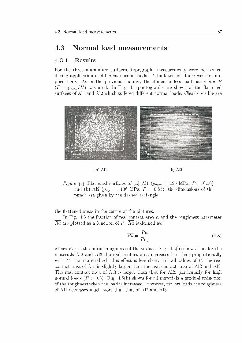
4.3. Normal load measurements 87
4.3 Normal load measurements
4.3.1 Results
For the three aluminium surfaces, topography measurements were performedduring application of di�erent normal loads. A bulk tension force was not ap-plied here. As in the previous chapter, the dimensionless load parameter P(P = pnom=H) was used. In Fig. 4.4 photographs are shown of the attenedsurfaces of Al1 and Al2 which su�ered di�erent normal loads. Clearly visible are
0.4 mm
0.4
mm
(a) Al1
0.4 mm
0.4
mm
(b) Al2
Figure 4.4: Flattened surfaces of (a) Al1 (pnom = 125 MPa, P = 0:16)and (b) Al2 (pnom = 136 MPa, P = 0:55); the dimensions of thepunch are given by the dashed rectangle.
the attened areas in the centre of the pictures.In Fig. 4.5 the fraction of real contact area � and the roughness parameter
Ra are plotted as a function of P . Ra is de�ned as:
Ra =Ra
Ra0(4.3)
where Ra0 is the initial roughness of the surface. Fig. 4.5(a) shows that for thematerials Al2 and Al3 the real contact area increases less than proportionallywith P . For material Al1 this e�ect is less clear. For all values of P , the realcontact area of Al1 is slightly larger than the real contact area of Al2 and Al3.The real contact area of Al3 is larger than that for Al2, particularly for highnormal loads (P > 0:3). Fig. 4.5(b) shows for all materials a gradual reductionof the roughness when the load is increased. However, for low loads the roughnessof Al1 decreases much more than that of Al2 and Al3.
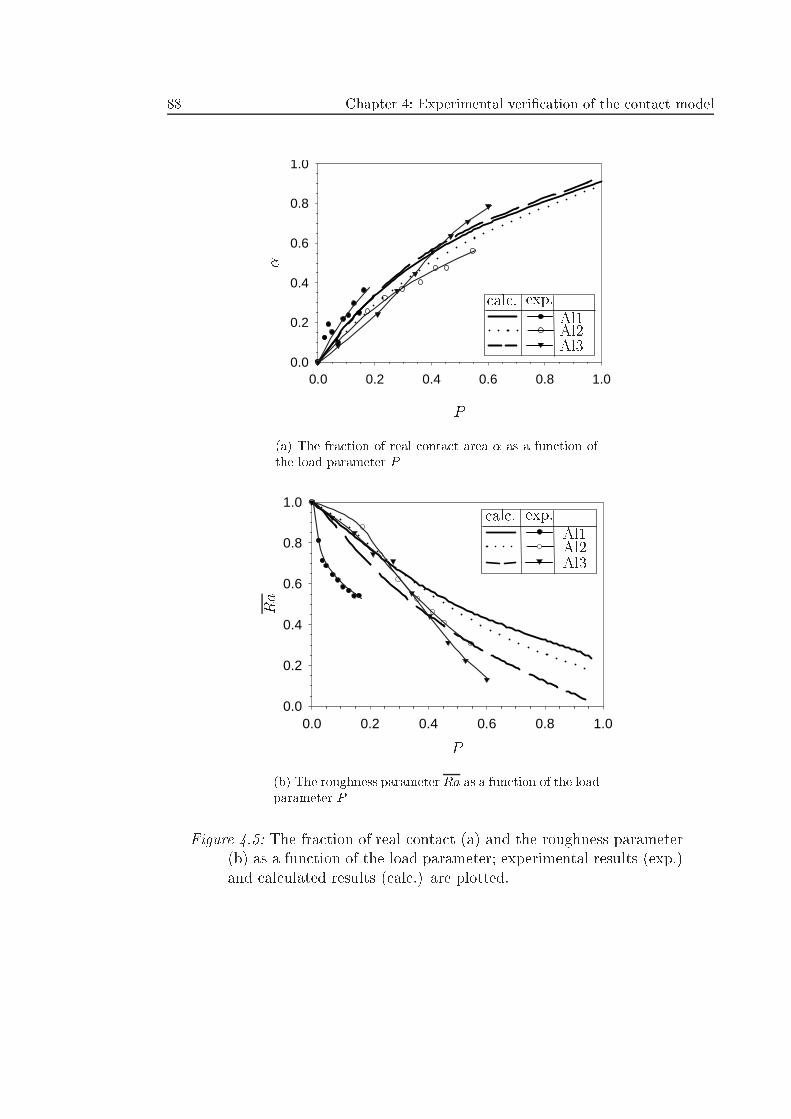
88 Chapter 4: Experimental veri�cation of the contact model
0.0 0.2 0.4 0.6 0.8 1.00.0
0.2
0.4
0.6
0.8
1.0
P
Al1Al2Al3
�
calc. exp.
(a) The fraction of real contact area � as a function ofthe load parameter P
0.0 0.2 0.4 0.6 0.8 1.00.0
0.2
0.4
0.6
0.8
1.0
P
Ra
Al1Al2Al3
calc. exp.
(b) The roughness parameter Ra as a function of the loadparameter P
Figure 4.5: The fraction of real contact (a) and the roughness parameter(b) as a function of the load parameter; experimental results (exp.)and calculated results (calc.) are plotted.
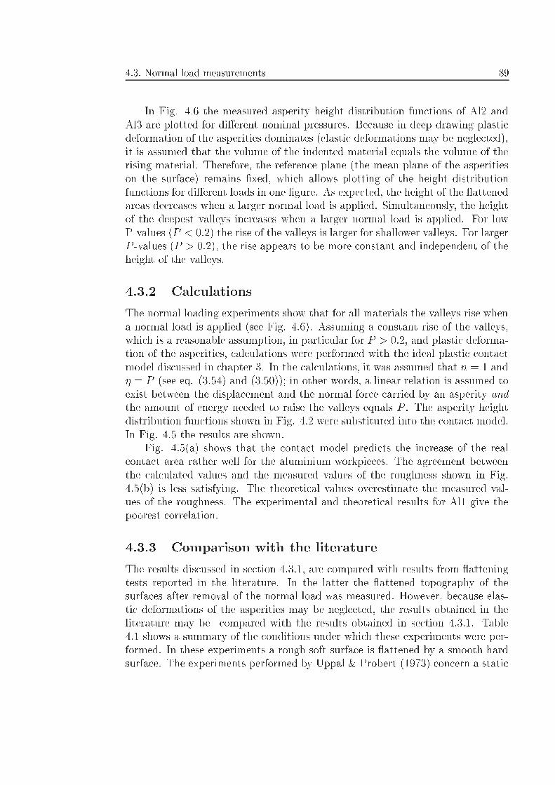
4.3. Normal load measurements 89
In Fig. 4.6 the measured asperity height distribution functions of Al2 andAl3 are plotted for di�erent nominal pressures. Because in deep drawing plasticdeformation of the asperities dominates (elastic deformations may be neglected),it is assumed that the volume of the indented material equals the volume of therising material. Therefore, the reference plane (the mean plane of the asperitieson the surface) remains �xed, which allows plotting of the height distributionfunctions for di�erent loads in one �gure. As expected, the height of the attenedareas decreases when a larger normal load is applied. Simultaneously, the heightof the deepest valleys increases when a larger normal load is applied. For lowP-values (P < 0:2) the rise of the valleys is larger for shallower valleys. For largerP -values (P > 0:2), the rise appears to be more constant and independent of theheight of the valleys.
4.3.2 Calculations
The normal loading experiments show that for all materials the valleys rise whena normal load is applied (see Fig. 4.6). Assuming a constant rise of the valleys,which is a reasonable assumption, in particular for P > 0:2, and plastic deforma-tion of the asperities, calculations were performed with the ideal plastic contactmodel discussed in chapter 3. In the calculations, it was assumed that n = 1 and� = P (see eq. (3.54) and (3.50)); in other words, a linear relation is assumed toexist between the displacement and the normal force carried by an asperity andthe amount of energy needed to raise the valleys equals P . The asperity heightdistribution functions shown in Fig. 4.2 were substituted into the contact model.In Fig. 4.5 the results are shown.
Fig. 4.5(a) shows that the contact model predicts the increase of the realcontact area rather well for the aluminium workpieces. The agreement betweenthe calculated values and the measured values of the roughness shown in Fig.4.5(b) is less satisfying. The theoretical values overestimate the measured val-ues of the roughness. The experimental and theoretical results for Al1 give thepoorest correlation.
4.3.3 Comparison with the literature
The results discussed in section 4.3.1, are compared with results from atteningtests reported in the literature. In the latter the attened topography of thesurfaces after removal of the normal load was measured. However, because elas-tic deformations of the asperities may be neglected, the results obtained in theliterature may be compared with the results obtained in section 4.3.1. Table4.1 shows a summary of the conditions under which these experiments were per-formed. In these experiments a rough soft surface is attened by a smooth hardsurface. The experiments performed by Uppal & Probert (1973) concern a static
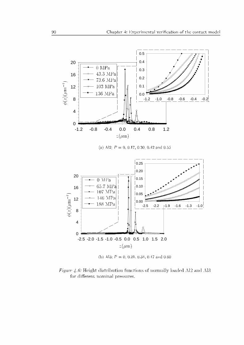
90 Chapter 4: Experimental veri�cation of the contact model
-1.2 -0.8 -0.4 0.0 0.4 0.8 1.20
4
8
12
16
20
-1.2 -1.0 -0.8 -0.6 -0.4 -0.20.0
0.1
0.2
0.3
0.4
0.5
z(�m)
�( z) (�m�1)
0 MPa
43.3 MPa
73.6 MPa
103 MPa
136 MPa
(a) Al2; P = 0, 0.17, 0.30, 0.42 and 0.55
-2.5 -2.0 -1.5 -1.0 -0.5 0.0 0.5 1.0 1.5 2.00
4
8
12
16
20
-2.5 -2.2 -1.9 -1.6 -1.3 -1.00.00
0.05
0.10
0.15
0.20
0.25
z(�m)
�( z)(�m�1)
0 MPa
65.7 MPa107 MPa146 MPa188 MPa
(b) Al3; P = 0, 0.21, 0.34, 0.47 and 0.60
Figure 4.6: Height distribution functions of normally loaded Al2 and Al3for di�erent nominal pressures.
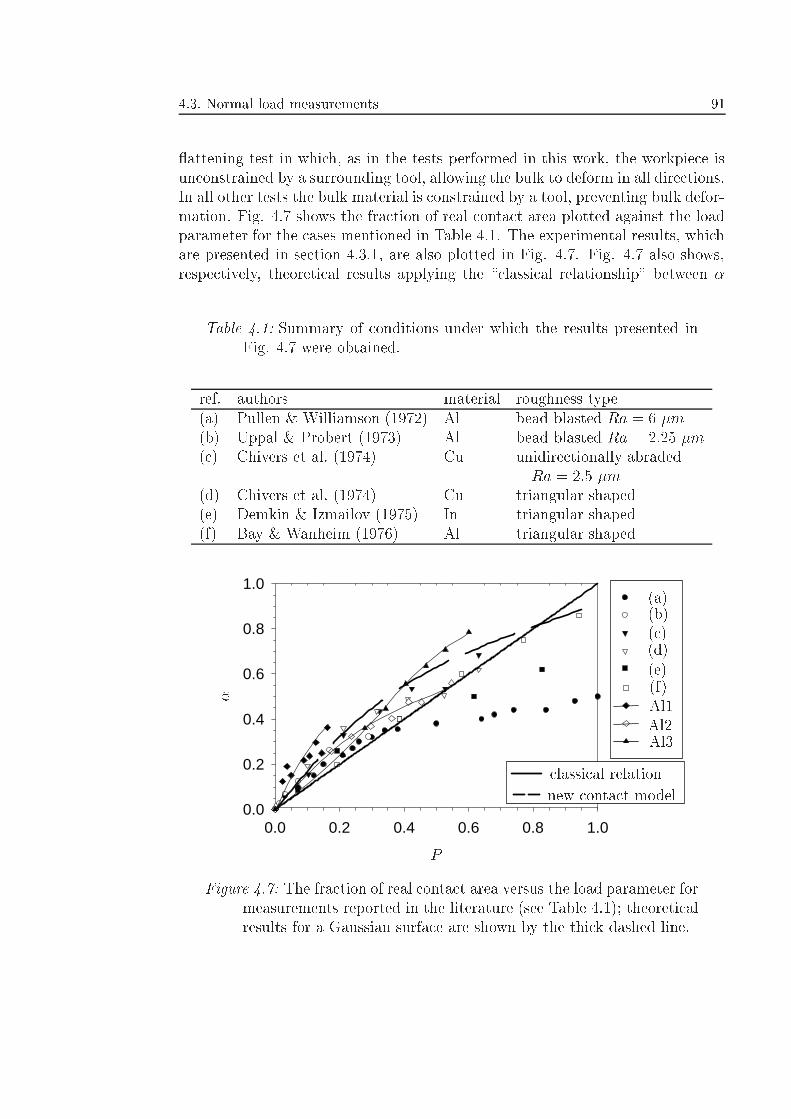
4.3. Normal load measurements 91
attening test in which, as in the tests performed in this work, the workpiece isunconstrained by a surrounding tool, allowing the bulk to deform in all directions.In all other tests the bulk material is constrained by a tool, preventing bulk defor-mation. Fig. 4.7 shows the fraction of real contact area plotted against the loadparameter for the cases mentioned in Table 4.1. The experimental results, whichare presented in section 4.3.1, are also plotted in Fig. 4.7. Fig. 4.7 also shows,respectively, theoretical results applying the \classical relationship" between �
Table 4.1: Summary of conditions under which the results presented inFig. 4.7 were obtained.
ref. authors material roughness type(a) Pullen & Williamson (1972) Al bead blasted Ra = 6 �m(b) Uppal & Probert (1973) Al bead blasted Ra = 2:25 �m(c) Chivers et al. (1974) Cu unidirectionally abraded
Ra = 2:5 �m(d) Chivers et al. (1974) Cu triangular shaped(e) Demkin & Izmailov (1975) In triangular shaped(f) Bay & Wanheim (1976) Al triangular shaped
0.0 0.2 0.4 0.6 0.8 1.00.0
0.2
0.4
0.6
0.8
1.0
P
�
(a)(b)(c)(d)(e)(f)Al1Al2Al3
classical relation
new contact model
Figure 4.7: The fraction of real contact area versus the load parameter formeasurements reported in the literature (see Table 4.1); theoreticalresults for a Gaussian surface are shown by the thick dashed line.
92 Chapter 4: Experimental veri�cation of the contact model
and P (� = pnom=H = P ) and the new contact model derived in section 3.2.1.The calculation with the new contact model was performed assuming a Gaussianheight distribution function of the workpiece for which the results are indepen-dent of the value of its standard deviation. From Fig. 4.7 it can be concludedthat with the possible exception of material Al1, the trend of all the experimentalresults is similar: the increase in real contact area is less than proportional to theload parameter. The \classical relationship" does not predict this non-linearityand underestimates the measured values of � for low values of P (P < 0:4). Forlarge values of P the classical relationship overestimates the results obtained byPullen & Williamson (1972) (a) and Demkin & Izmailov (1975) (e). The newcontact model predicts the fraction of real contact area better than the \classicalrelation" and it also includes the non-linearity between � and P . However, someexperimental results obtained by Pullen & Williamson (1972) (a) and Demkin &Izmailov (1975) (e), give lower values of � than predicted for reasons which arenot fully understood.
The rise of the valleys of a soft surface when a low normal load is applied,was also found by Uppal & Probert (1972) by performing indentation tests onsingle- and multi-asperity surfaces. It was found that for P < 1:0 the rise of deepvalleys was less than for shallow valleys. In the present work the same trend wasmeasured for P < 0:2, but for P > 0:2, a uniform rise was detected, agreeingwith the results published by Pullen & Williamson (1972).
4.4 Stretching measurements
In deep drawing processes bulk deformation of the workpiece occurs under dif-ferent conditions (see Fig. 1.3). In the ange region the material is hardlystretched during the application of the low nominal pressure applied by loadingthe blankholder. In the die rounding and punch radius regions, the strains in thematerial and the nominal pressure are large. On the ank of the punch, bulkdeformation occurs without a normal load.
In this section the in uence of the presence of a bulk strain on the topog-raphy of the surface is studied experimentally. The applied bulk deformation isuni-axial. In deep drawing processes the deformation of real three-dimensionalproducts is more complicated and deformations occur in all three directions. How-ever, when the asperities of the sheet material are unconstrained by a tool duringstretching (i.e., free deformation), Dautzenberg & Kals (1985) showed that whenthe e�ective strain is used as the governing parameter, the roughness of the sheetis independent of the deformation mode. On the contrary, when a normal loadand a tension force are applied simultaneously, the roughness depends on the de-formation mode. This is, for example, illustrated by the di�erent strain-contactmodels for plane stress deforming asperities (Wilson & Sheu (1988)) and plane
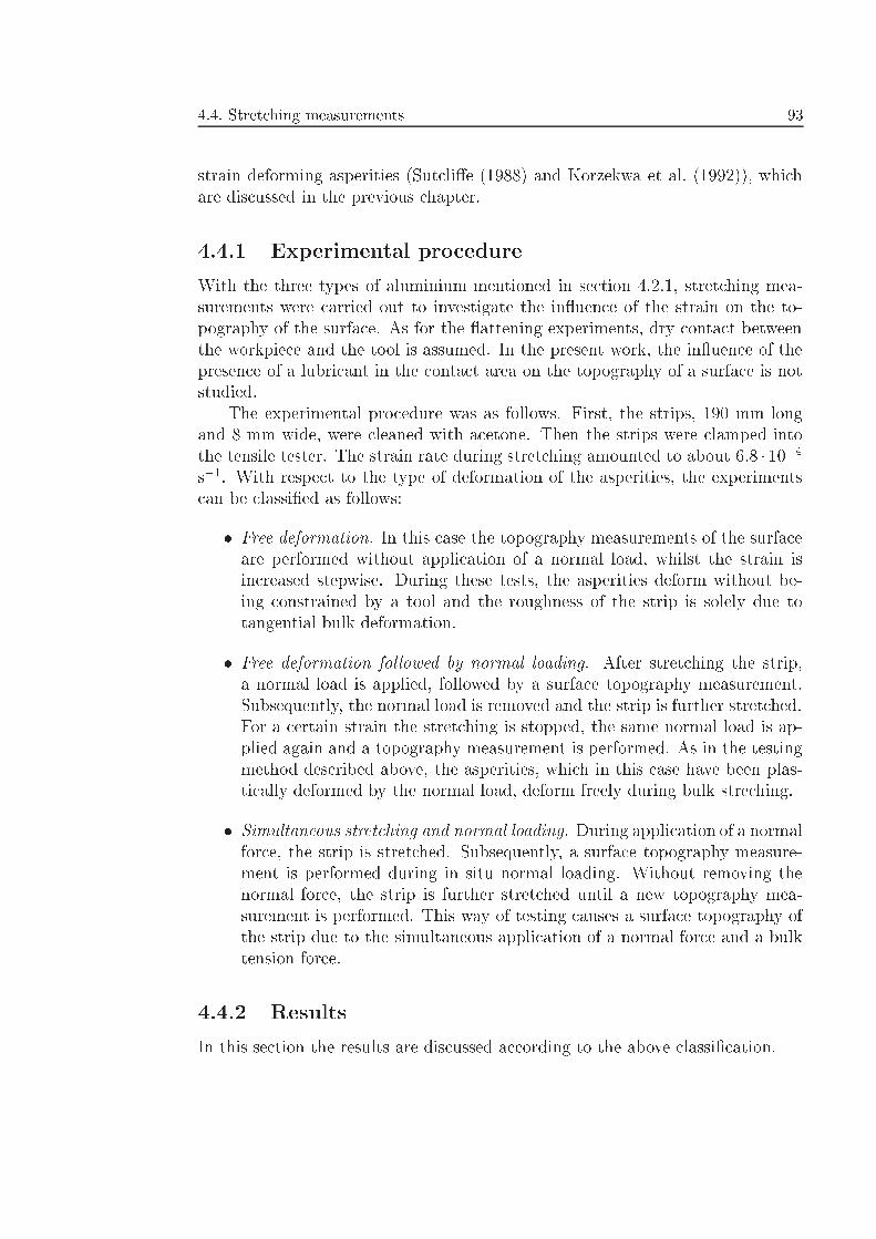
4.4. Stretching measurements 93
strain deforming asperities (Sutcli�e (1988) and Korzekwa et al. (1992)), whichare discussed in the previous chapter.
4.4.1 Experimental procedure
With the three types of aluminium mentioned in section 4.2.1, stretching mea-surements were carried out to investigate the in uence of the strain on the to-pography of the surface. As for the attening experiments, dry contact betweenthe workpiece and the tool is assumed. In the present work, the in uence of thepresence of a lubricant in the contact area on the topography of a surface is notstudied.
The experimental procedure was as follows. First, the strips, 190 mm longand 8 mm wide, were cleaned with acetone. Then the strips were clamped intothe tensile tester. The strain rate during stretching amounted to about 6:8 � 10�4s�1. With respect to the type of deformation of the asperities, the experimentscan be classi�ed as follows:
� Free deformation. In this case the topography measurements of the surfaceare performed without application of a normal load, whilst the strain isincreased stepwise. During these tests, the asperities deform without be-ing constrained by a tool and the roughness of the strip is solely due totangential bulk deformation.
� Free deformation followed by normal loading. After stretching the strip,a normal load is applied, followed by a surface topography measurement.Subsequently, the normal load is removed and the strip is further stretched.For a certain strain the stretching is stopped, the same normal load is ap-plied again and a topography measurement is performed. As in the testingmethod described above, the asperities, which in this case have been plas-tically deformed by the normal load, deform freely during bulk streching.
� Simultaneous stretching and normal loading. During application of a normalforce, the strip is stretched. Subsequently, a surface topography measure-ment is performed during in situ normal loading. Without removing thenormal force, the strip is further stretched until a new topography mea-surement is performed. This way of testing causes a surface topography ofthe strip due to the simultaneous application of a normal force and a bulktension force.
4.4.2 Results
In this section the results are discussed according to the above classi�cation.
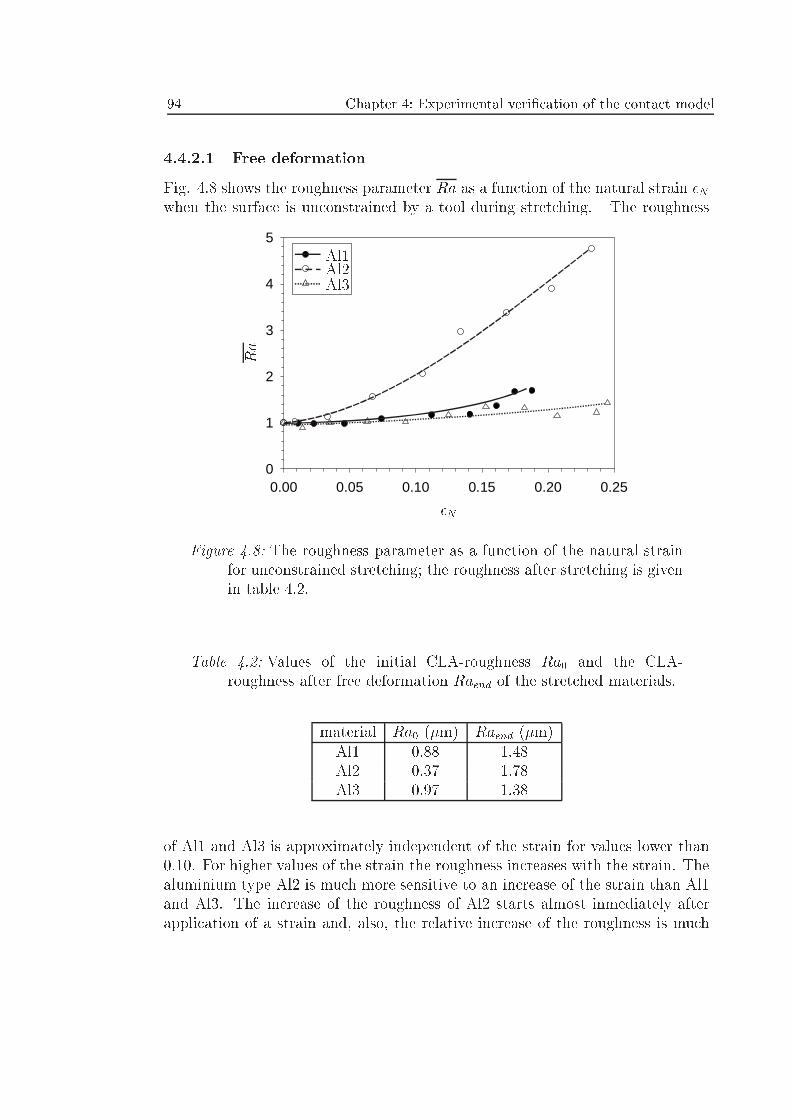
94 Chapter 4: Experimental veri�cation of the contact model
4.4.2.1 Free deformation
Fig. 4.8 shows the roughness parameter Ra as a function of the natural strain �Nwhen the surface is unconstrained by a tool during stretching. The roughness
0.00 0.05 0.10 0.15 0.20 0.250
1
2
3
4
5
�N
Ra
Al1Al2Al3
Figure 4.8: The roughness parameter as a function of the natural strainfor unconstrained stretching; the roughness after stretching is givenin table 4.2.
Table 4.2: Values of the initial CLA-roughness Ra0 and the CLA-roughness after free deformation Raend of the stretched materials.
material Ra0 (�m) Raend (�m)Al1 0.88 1.48Al2 0.37 1.78Al3 0.97 1.38
of Al1 and Al3 is approximately independent of the strain for values lower than0.10. For higher values of the strain the roughness increases with the strain. Thealuminium type Al2 is much more sensitive to an increase of the strain than Al1and Al3. The increase of the roughness of Al2 starts almost inmediately afterapplication of a strain and, also, the relative increase of the roughness is much
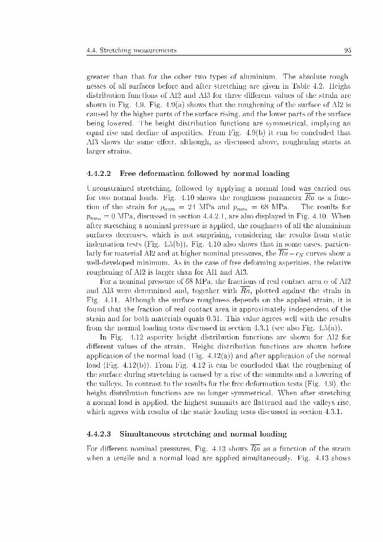
4.4. Stretching measurements 95
greater than that for the other two types of aluminium. The absolute rough-nesses of all surfaces before and after stretching are given in Table 4.2. Heightdistribution functions of Al2 and Al3 for three di�erent values of the strain areshown in Fig. 4.9. Fig. 4.9(a) shows that the roughening of the surface of Al2 iscaused by the higher parts of the surface rising, and the lower parts of the surfacebeing lowered. The height distribution functions are symmetrical, implying anequal rise and decline of asperities. From Fig. 4.9(b) it can be concluded thatAl3 shows the same e�ect, although, as discussed above, roughening starts atlarger strains.
4.4.2.2 Free deformation followed by normal loading
Unconstrained stretching, followed by applying a normal load was carried outfor two normal loads. Fig. 4.10 shows the roughness parameter Ra as a func-tion of the strain for pnom = 24 MPa and pnom = 68 MPa. The results forpnom = 0 MPa, discussed in section 4.4.2.1, are also displayed in Fig. 4.10. Whenafter stretching a nominal pressure is applied, the roughness of all the aluminiumsurfaces decreases, which is not surprising, considering the results from staticindentation tests (Fig. 4.5(b)). Fig. 4.10 also shows that in some cases, particu-larly for material Al2 and at higher nominal pressures, the Ra��N curves show awell-developed minimum. As in the case of free deforming asperities, the relativeroughening of Al2 is larger than for Al1 and Al3.
For a nominal pressure of 68 MPa, the fractions of real contact area � of Al2and Al3 were determined and, together with Ra, plotted against the strain inFig. 4.11. Although the surface roughness depends on the applied strain, it isfound that the fraction of real contact area is approximately independent of thestrain and for both materials equals 0.31. This value agrees well with the resultsfrom the normal loading tests discussed in section 4.3.1 (see also Fig. 4.5(a)).
In Fig. 4.12 asperity height distribution functions are shown for Al2 fordi�erent values of the strain. Height distribution functions are shown beforeapplication of the normal load (Fig. 4.12(a)) and after application of the normalload (Fig. 4.12(b)). From Fig. 4.12 it can be concluded that the roughening ofthe surface during stretching is caused by a rise of the summits and a lowering ofthe valleys. In contrast to the results for the free deformation tests (Fig. 4.9), theheight distribution functions are no longer symmetrical. When after stretchinga normal load is applied, the highest summits are attened and the valleys rise,which agrees with results of the static loading tests discussed in section 4.3.1.
4.4.2.3 Simultaneous stretching and normal loading
For di�erent nominal pressures, Fig. 4.13 shows Ra as a function of the strainwhen a tensile and a normal load are applied simultaneously. Fig. 4.13 shows
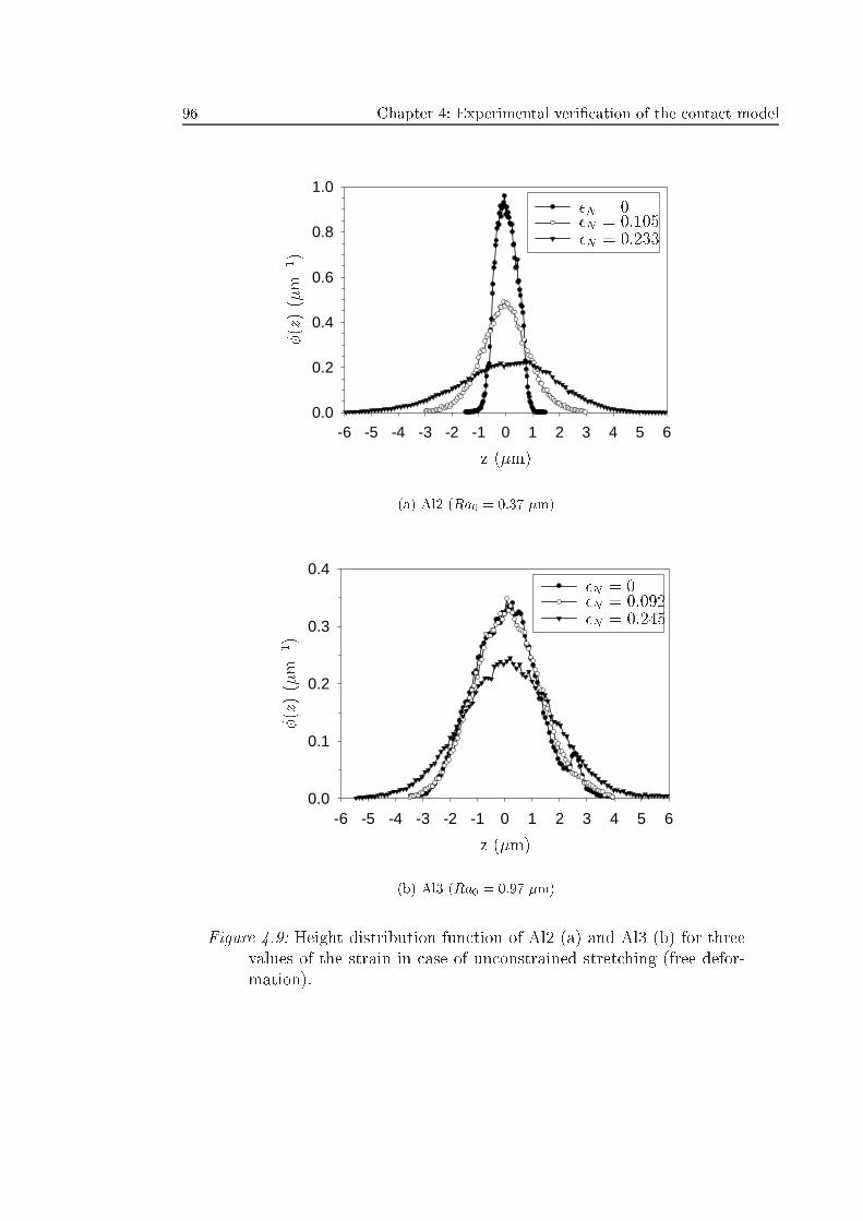
96 Chapter 4: Experimental veri�cation of the contact model
-6 -5 -4 -3 -2 -1 0 1 2 3 4 5 60.0
0.2
0.4
0.6
0.8
1.0
z (�m)
�(z)(�m�1)
�N = 0�N = 0:105�N = 0:233
(a) Al2 (Ra0 = 0:37 �m)
-6 -5 -4 -3 -2 -1 0 1 2 3 4 5 60.0
0.1
0.2
0.3
0.4
z (�m)
�(z)(�m�1)
�N = 0�N = 0:092�N = 0:245
(b) Al3 (Ra0 = 0:97 �m)
Figure 4.9: Height distribution function of Al2 (a) and Al3 (b) for threevalues of the strain in case of unconstrained stretching (free defor-mation).
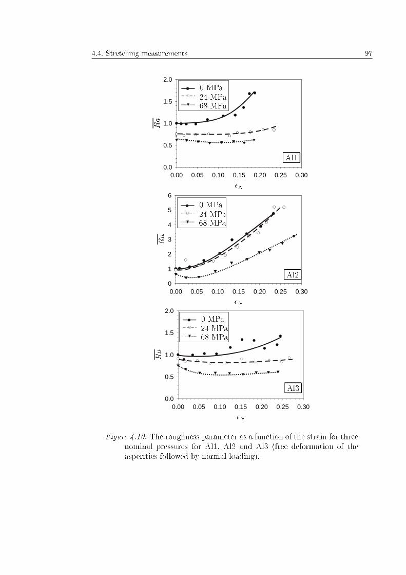
4.4. Stretching measurements 97
0.00 0.05 0.10 0.15 0.20 0.25 0.300.0
0.5
1.0
1.5
2.0
0.00 0.05 0.10 0.15 0.20 0.25 0.300
1
2
3
4
5
6
0.00 0.05 0.10 0.15 0.20 0.25 0.300.0
0.5
1.0
1.5
2.0
�N
�N
�N
Ra
Ra
Ra
0 MPa
0 MPa
0 MPa
24 MPa
24 MPa
24 MPa
68 MPa
68 MPa
68 MPa
Al1
Al2
Al3
Figure 4.10: The roughness parameter as a function of the strain for threenominal pressures for Al1, Al2 and Al3 (free deformation of theasperities followed by normal loading).
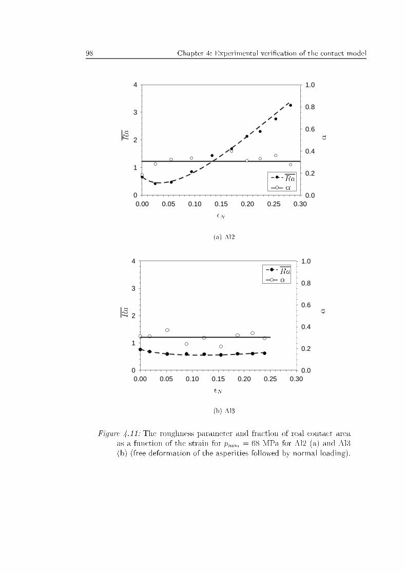
98 Chapter 4: Experimental veri�cation of the contact model
0.0
0.2
0.4
0.6
0.8
1.0
0.00 0.05 0.10 0.15 0.20 0.25 0.300
1
2
3
4
�N
Ra
Ra
�
�
(a) Al2
Plot 1Plot 1
0.0
0.2
0.4
0.6
0.8
1.0
0.00 0.05 0.10 0.15 0.20 0.25 0.300
1
2
3
4
�N
Ra
Ra
�
�
(b) Al3
Figure 4.11: The roughness parameter and fraction of real contact areaas a function of the strain for pnom = 68 MPa for Al2 (a) and Al3(b) (free deformation of the asperities followed by normal loading).
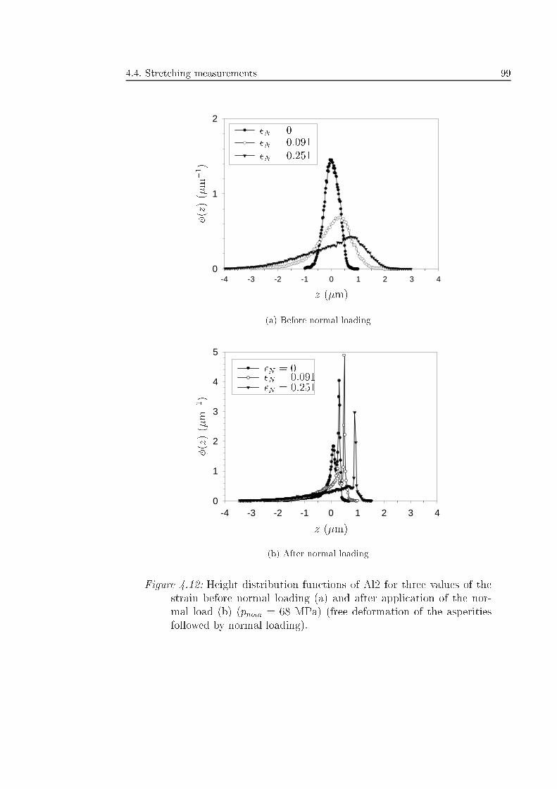
4.4. Stretching measurements 99
-4 -3 -2 -1 0 1 2 3 40
1
2
z (�m)
�( z)(�m�1)
�N = 0�N = 0:091�N = 0:251
(a) Before normal loading
-4 -3 -2 -1 0 1 2 3 40
1
2
3
4
5
z (�m)
�(z)(�m�1)
�N = 0�N = 0:091�N = 0:251
(b) After normal loading
Figure 4.12: Height distribution functions of Al2 for three values of thestrain before normal loading (a) and after application of the nor-mal load (b) (pnom = 68 MPa) (free deformation of the asperitiesfollowed by normal loading).
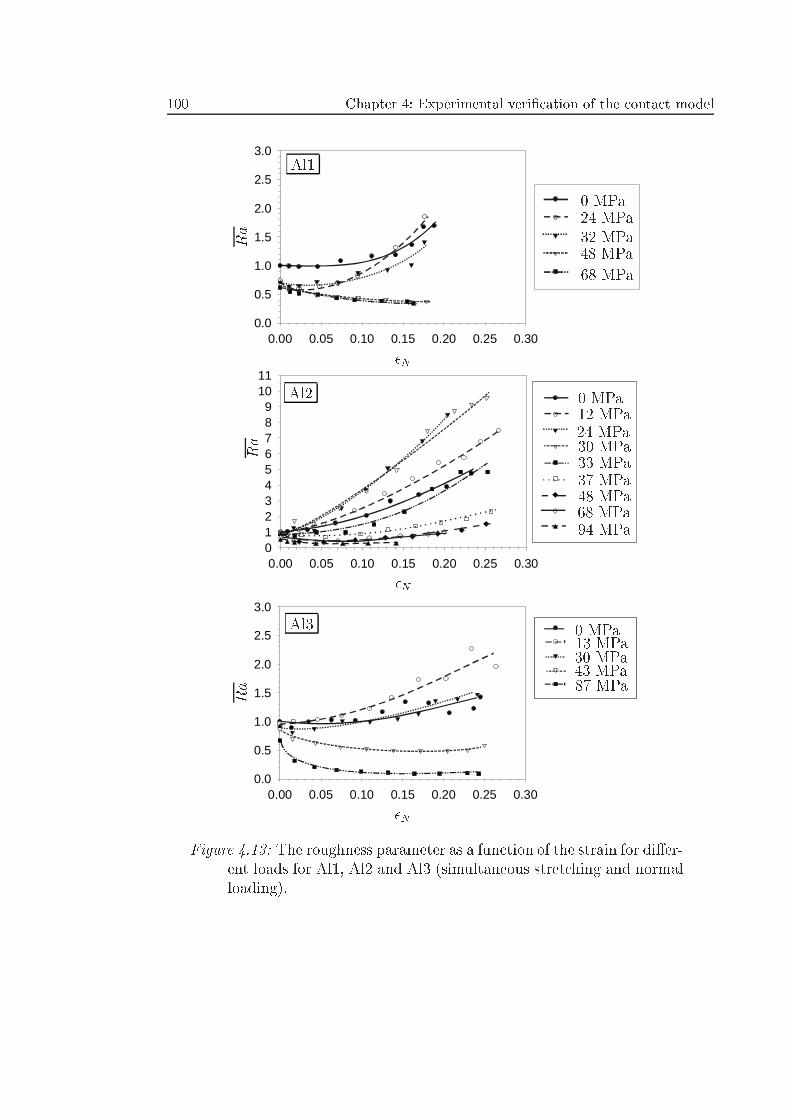
100 Chapter 4: Experimental veri�cation of the contact model
0.00 0.05 0.10 0.15 0.20 0.25 0.300.0
0.5
1.0
1.5
2.0
2.5
3.0
0.00 0.05 0.10 0.15 0.20 0.25 0.300123456789
1011
0.00 0.05 0.10 0.15 0.20 0.25 0.300.0
0.5
1.0
1.5
2.0
2.5
3.0
�N
�N
�N
Ra
Ra
Ra
0 MPa24 MPa32 MPa48 MPa
68 MPa
0 MPa12 MPa24 MPa30 MPa33 MPa37 MPa48 MPa68 MPa94 MPa
0 MPa13 MPa30 MPa43 MPa87 MPa
Al1
Al2
Al3
Figure 4.13: The roughness parameter as a function of the strain for di�er-ent loads for Al1, Al2 and Al3 (simultaneous stretching and normalloading).
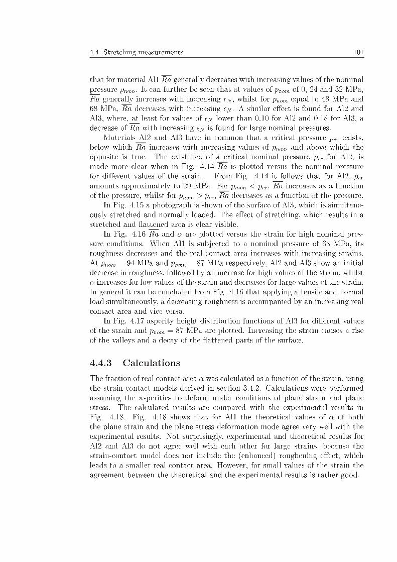
4.4. Stretching measurements 101
that for material Al1 Ra generally decreases with increasing values of the nominalpressure pnom. It can further be seen that at values of pnom of 0, 24 and 32 MPa,Ra generally increases with increasing �N , whilst for pnom equal to 48 MPa and68 MPa, Ra decreases with increasing �N . A similar e�ect is found for Al2 andAl3, where, at least for values of �N lower than 0.10 for Al2 and 0.18 for Al3, adecrease of Ra with increasing �N is found for large nominal pressures.
Materials Al2 and Al3 have in common that a critical pressure pcr exists,below which Ra increases with increasing values of pnom and above which theopposite is true. The existence of a critical nominal pressure pcr for Al2, ismade more clear when in Fig. 4.14 Ra is plotted versus the nominal pressurefor di�erent values of the strain. From Fig. 4.14 it follows that for Al2, pcramounts approximately to 29 MPa. For pnom < pcr, Ra increases as a functionof the pressure, whilst for pnom > pcr, Ra decreases as a function of the pressure.
In Fig. 4.15 a photograph is shown of the surface of Al3, which is simultane-ously stretched and normally loaded. The e�ect of stretching, which results in astretched and attened area is clear visible.
In Fig. 4.16 Ra and � are plotted versus the strain for high nominal pres-sure conditions. When Al1 is subjected to a nominal pressure of 68 MPa, itsroughness decreases and the real contact area increases with increasing strains.At pnom = 94 MPa and pnom = 87 MPa respectively, Al2 and Al3 show an initialdecrease in roughness, followed by an increase for high values of the strain, whilst� increases for low values of the strain and decreases for large values of the strain.In general it can be concluded from Fig. 4.16 that applying a tensile and normalload simultaneously, a decreasing roughness is accompanied by an increasing realcontact area and vice versa.
In Fig. 4.17 asperity height distribution functions of Al3 for di�erent valuesof the strain and pnom = 87 MPa are plotted. Increasing the strain causes a riseof the valleys and a decay of the attened parts of the surface.
4.4.3 Calculations
The fraction of real contact area � was calculated as a function of the strain, usingthe strain-contact models derived in section 3.4.2. Calculations were performedassuming the asperities to deform under conditions of plane strain and planestress. The calculated results are compared with the experimental results inFig. 4.18. Fig. 4.18 shows that for Al1 the theoretical values of � of boththe plane strain and the plane stress deformation mode agree very well with theexperimental results. Not surprisingly, experimental and theoretical results forAl2 and Al3 do not agree well with each other for large strains, because thestrain-contact model does not include the (enhanced) roughening e�ect, whichleads to a smaller real contact area. However, for small values of the strain theagreement between the theoretical and the experimental results is rather good.
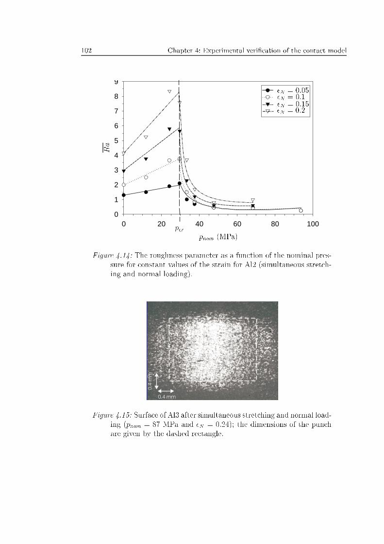
102 Chapter 4: Experimental veri�cation of the contact model
0 20 40 60 80 1000
1
2
3
4
5
6
7
8
9
pnom (MPa)
Ra
�N = 0:05�N = 0:1�N = 0:15�N = 0:2
pcr
Figure 4.14: The roughness parameter as a function of the nominal pres-sure for constant values of the strain for Al2 (simultaneous stretch-ing and normal loading).
0.4 mm
0.4
mm
Figure 4.15: Surface of Al3 after simultaneous stretching and normal load-ing (pnom = 87 MPa and �N = 0:24); the dimensions of the punchare given by the dashed rectangle.
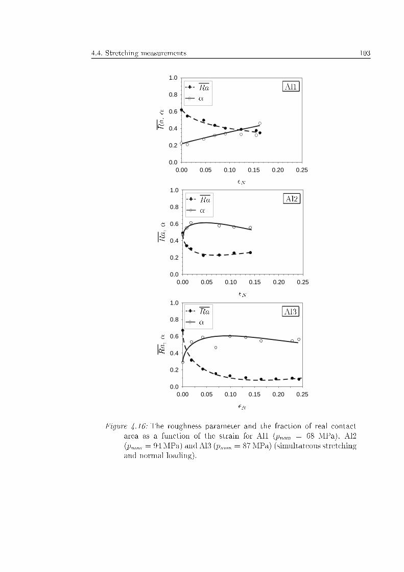
4.4. Stretching measurements 103
0.00 0.05 0.10 0.15 0.20 0.250.0
0.2
0.4
0.6
0.8
1.0
0.00 0.05 0.10 0.15 0.20 0.250.0
0.2
0.4
0.6
0.8
1.0
0.00 0.05 0.10 0.15 0.20 0.250.0
0.2
0.4
0.6
0.8
1.0
�N
�N
�N
Ra,�
Ra,�
Ra,�
Ra
Ra
Ra
�
�
�
Al1
Al2
Al3
Figure 4.16: The roughness parameter and the fraction of real contactarea as a function of the strain for Al1 (pnom = 68 MPa), Al2(pnom = 94 MPa) and Al3 (pnom = 87 MPa) (simultateous stretchingand normal loading).
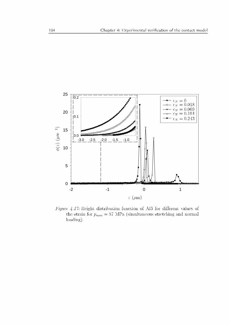
104 Chapter 4: Experimental veri�cation of the contact model
-2 -1 0 10
5
10
15
20
25
-3.0 -2.5 -2.0 -1.5 -1.00.0
0.1
0.2
z (�m)
�( z)(�m�1)
�N = 0�N = 0:018�N = 0:069�N = 0:164�N = 0:243
Figure 4.17: Height distribution function of Al3 for di�erent values ofthe strain for pnom = 87 MPa (simultaneous stretching and normalloading).
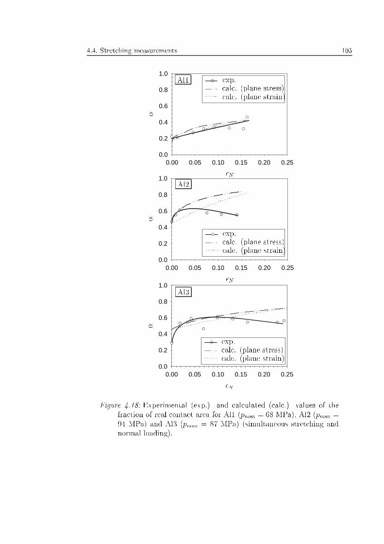
4.4. Stretching measurements 105
0.00 0.05 0.10 0.15 0.20 0.250.0
0.2
0.4
0.6
0.8
1.0
0.00 0.05 0.10 0.15 0.20 0.250.0
0.2
0.4
0.6
0.8
1.0
0.00 0.05 0.10 0.15 0.20 0.250.0
0.2
0.4
0.6
0.8
1.0
�N
�N
�N
�
�
�
exp.
exp.
exp.
calc. (plane stress)
calc. (plane stress)
calc. (plane stress)
calc. (plane strain)
calc. (plane strain)
calc. (plane strain)
Al1
Al2
Al3
Figure 4.18: Experimental (exp.) and calculated (calc.) values of thefraction of real contact area for Al1 (pnom = 68 MPa), Al2 (pnom =94 MPa) and Al3 (pnom = 87 MPa) (simultaneous stretching andnormal loading).
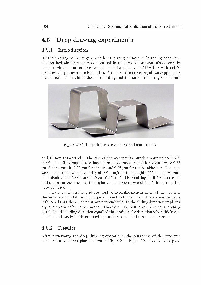
106 Chapter 4: Experimental veri�cation of the contact model
4.5 Deep drawing experiments
4.5.1 Introduction
It is interesting to investigate whether the roughening and attening behaviourof stretched aluminium strips discussed in the previous section, also occurs indeep drawing operations. Rectangular-hat-shaped cups of Al2 with a width of 50mm were deep drawn (see Fig. 4.19). A mineral deep drawing oil was applied forlubrication. The radii of the die rounding and the punch rounding were 5 mm
Figure 4.19: Deep drawn rectangular-had-shaped cups.
and 10 mm respectively. The size of the rectangular punch amounted to 70x70mm2. The CLA-roughness values of the tools measured with a stylus, were 0.78�m for the punch, 0.30 �m for the die and 0.26 �m for the blankholder. The cupswere deep drawn with a velocity of 100 mm/min to a height of 55 mm or 80 mm.The blankholder forces varied from 10 kN to 50 kN resulting in di�erent stressesand strains in the cups. At the highest blankholder force of 50 kN fracture of thecups occurred.
On some strips a �ne grid was applied to enable measurement of the strain atthe surface accurately with computer based software. From these measurementsit followed that there was no strain perpendicular to the sliding direction implyinga plane strain deformation mode. Therefore, the bulk strain due to stretchingparallel to the sliding direction equalled the strain in the direction of the thickness,which could easily be determined by an ultrasonic thickness measurement.
4.5.2 Results
After performing the deep drawing operations, the roughness of the cups wasmeasured at di�erent places shown in Fig. 4.21. Fig. 4.20 shows contour plots
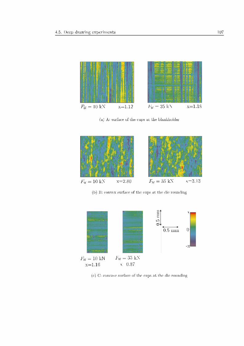
4.5. Deep drawing experiments 107
Fbl = 10 kN x=1.12 Fbl = 35 kN x=1.18
(a) A: surface of the cups at the blankholder
Fbl = 10 kN x=2.80 Fbl = 35 kN x=3.13
(b) B: convex surface of the cups at the die rounding
Fbl = 10 kN
x=1.16
Fbl = 35 kN
x=0.87
x
0
-x
0.5 mm
0.5mm
(c) C: concave surface of the cups at the die rounding
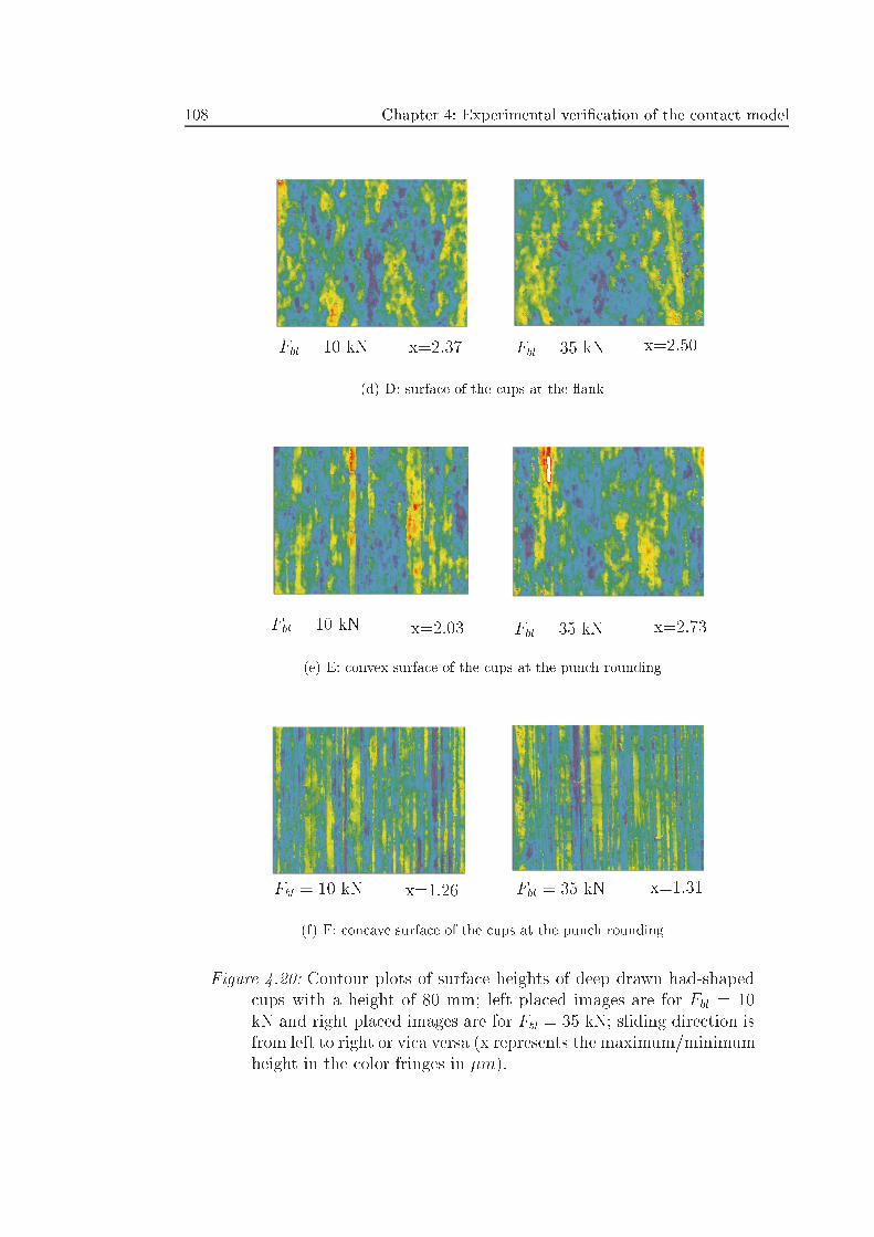
108 Chapter 4: Experimental veri�cation of the contact model
Fbl = 10 kN x=2.37 Fbl = 35 kN x=2.50
(d) D: surface of the cups at the ank
Fbl = 10 kN x=2.03 Fbl = 35 kN x=2.73
(e) E: convex surface of the cups at the punch rounding
Fbl = 10 kN x=1.26 Fbl = 35 kN x=1.31
(f) F: concave surface of the cups at the punch rounding
Figure 4.20: Contour plots of surface heights of deep drawn had-shapedcups with a height of 80 mm; left placed images are for Fbl = 10kN and right placed images are for Fbl = 35 kN; sliding direction isfrom left to right or vica versa (x represents the maximum/minimumheight in the color fringes in �m).
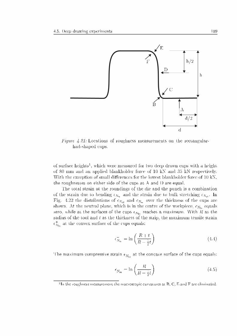
4.5. Deep drawing experiments 109
AB
C
D
E
F
d/2
d
h
h/2
Figure 4.21: Locations of roughness measurements on the rectangular-had-shaped cups.
of surface heights1, which were measured for two deep drawn cups with a heightof 80 mm and an applied blankholder force of 10 kN and 35 kN respectively.With the exception of small di�erences for the lowest blankholder force of 10 kN,the roughnesses on either side of the cups at A and D are equal.
The total strain at the roundings of the die and the punch is a combinationof the strain due to bending �Nbe
and the strain due to bulk stretching �Nst . InFig. 4.22 the distributions of �Nst and �Nbe
over the thickness of the cups areshown. At the neutral plane, which is in the centre of the workpiece, �Nbe
equalszero, while at the surfaces of the cups �Nbe
reaches a maximum. With R as theradius of the tool and t as the thickness of the strip, the maximum tensile strain�+Nbe
at the convex surface of the cups equals:
�+Nbe= ln
�R + t
R + 1
2t
�(4.4)
The maximum compressive strain ��Nbeat the concave surface of the cups equals:
��Nbe= ln
�R
R + 1
2t
�(4.5)
1In the roughness measurement the macroscopic curvatures at B, C, E and F are eliminated.
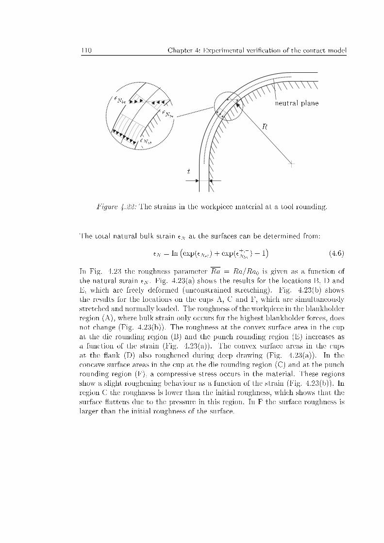
110 Chapter 4: Experimental veri�cation of the contact model
R
t
�+Nbe
��Nbe
�Nst
neutral plane
Figure 4.22: The strains in the workpiece material at a tool rounding.
The total natural bulk strain �N at the surfaces can be determined from:
�N = ln�exp(�Nst) + exp(�+;�Nbe
) + 1�
(4.6)
In Fig. 4.23 the roughness parameter Ra = Ra=Ra0 is given as a function ofthe natural strain �N . Fig. 4.23(a) shows the results for the locations B, D andE, which are freely deformed (unconstrained stretching). Fig. 4.23(b) showsthe results for the locations on the cups A, C and F, which are simultaneouslystretched and normally loaded. The roughness of the workpiece in the blankholderregion (A), where bulk strain only occurs for the highest blankholder forces, doesnot change (Fig. 4.23(b)). The roughness at the convex surface area in the cupat the die rounding region (B) and the punch rounding region (E) increases asa function of the strain (Fig. 4.23(a)). The convex surface areas in the cupsat the ank (D) also roughened during deep drawing (Fig. 4.23(a)). In theconcave surface areas in the cup at the die rounding region (C) and at the punchrounding region (F), a compressive stress occurs in the material. These regionsshow a slight roughening behaviour as a function of the strain (Fig. 4.23(b)). Inregion C the roughness is lower than the initial roughness, which shows that thesurface attens due to the pressure in this region. In F the surface roughness islarger than the initial roughness of the surface.
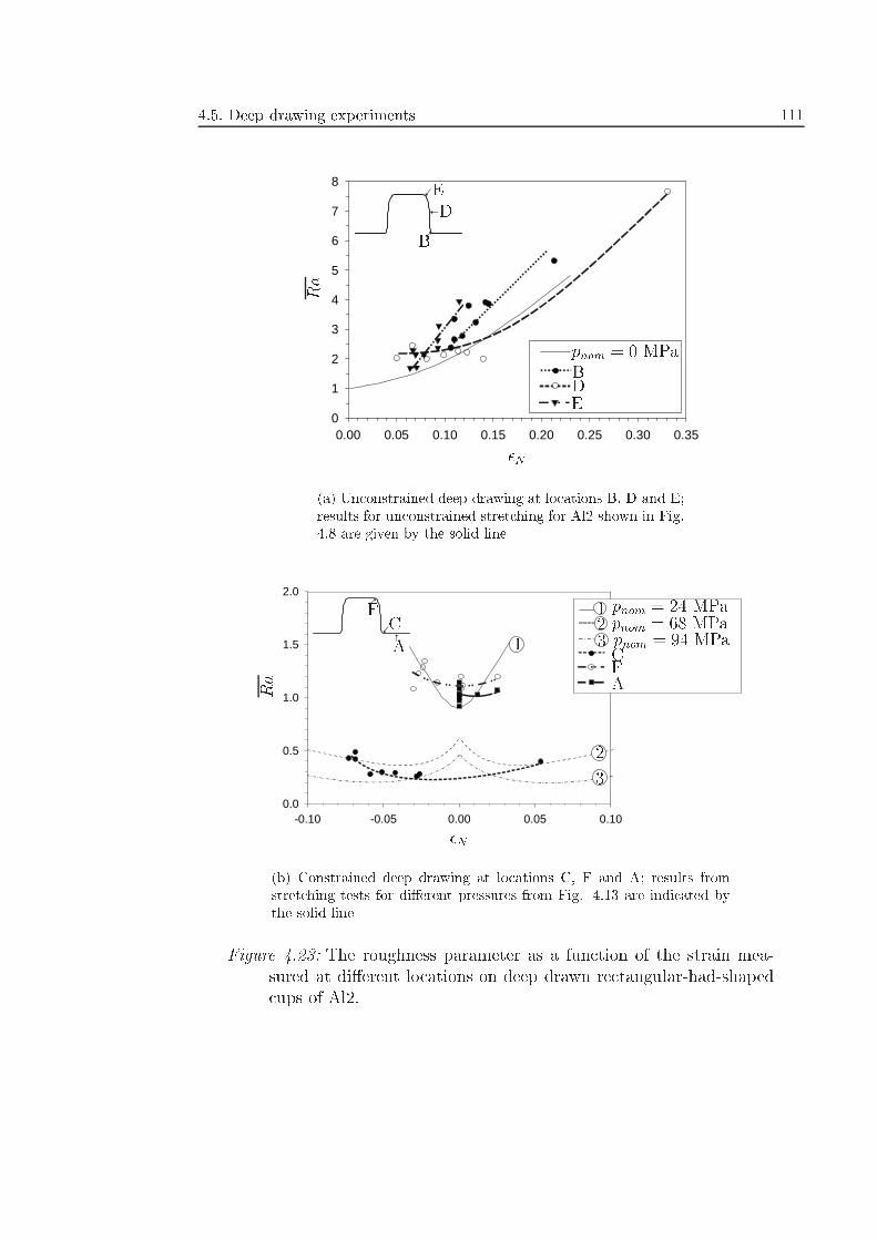
4.5. Deep drawing experiments 111
0.00 0.05 0.10 0.15 0.20 0.25 0.30 0.350
1
2
3
4
5
6
7
8
�N
Ra
B
B
D
D
E
E
pnom = 0 MPa
(a) Unconstrained deep drawing at locations B, D and E;results for unconstrained stretching for Al2 shown in Fig.4.8 are given by the solid line
-0.10 -0.05 0.00 0.05 0.100.0
0.5
1.0
1.5
2.0
�N
Ra
C
C
F
FA
A
pnom = 24 MPapnom = 68 MPapnom = 94 MPa
1
12
2
3
3
(b) Constrained deep drawing at locations C, F and A; results fromstretching tests for di�erent pressures from Fig. 4.13 are indicated bythe solid line
Figure 4.23: The roughness parameter as a function of the strain mea-sured at di�erent locations on deep drawn rectangular-had-shapedcups of Al2.
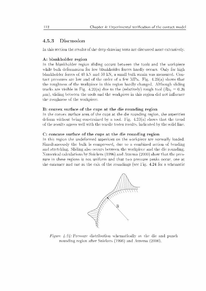
112 Chapter 4: Experimental veri�cation of the contact model
4.5.3 Discussion
In this section the results of the deep drawing tests are discussed more extensively.
A: blankholder regionIn the blankholder region sliding occurs between the tools and the workpiecewhile bulk deformation for low blankholder forces hardly occurs. Only for highblankholder forces of 40 kN and 50 kN, a small bulk strain was measured. Con-tact pressures are low and of the order of a few MPa. Fig. 4.23(a) shows thatthe roughness of the workpiece in this region hardly changed. Although slidingtracks are visible in Fig. 4.20(a) due to the (relatively) rough tool (Rat = 0.26�m), sliding between the tools and the workpiece in this region did not in uencethe roughness of the workpiece.
B: convex surface of the cups at the die rounding regionIn the convex surface area of the cups at the die rounding region, the asperitiesdeform without being constrained by a tool. Fig. 4.23(a) shows that the trendof the results agrees well with the tensile tester results, indicated by the solid line.
C: concave surface of the cups at the die rounding regionIn this region the undeformed asperities on the workpiece are normally loaded.Simultaneously the bulk is compressed, due to a combined action of bendingand stretching. Sliding also occurs between the workpiece and the die rounding.Numerical calculations by Sniekers (1996) and Atzema (2000) show that the pres-sure in these regions is not uniform and that two pressure peaks occur, one atthe entrance and one at the exit of the roundings (see Fig. 4.24 for a schematic
R
Figure 4.24: Pressure distribution schematically at the die and punchrounding region after Sniekers (1996) and Atzema (2000).
4.6. Discussion of results 113
view). When it is assumed that the deep drawing results may be compared withthe tensile tester results, i.e., the in uence of sliding on the topography is ne-glected, an estimation of the value of the pressure peak can be made. Comparingthe results for region C plotted in Fig. 4.23(b) with Fig. 4.13, the value of the�rst pressure peak is between 68 and 94 MPa. Because of the pressure peak, theroughness of the surface decreases and attening occurs (see also Fig. 4.20(c)).Because the material is hardly in real physical contact with the die rounding inthe centre (where the roughness measurement is performed), the strip roughenswith increasing strain because of the combined e�ect of bending and bulk stretch-ing. These results show that a compressive strain also results in roughening.
D: the ankIn Fig. 4.23(a) it is shown that, for strains between 0.05 and 0.15, the roughnessat the ank, which is twice the initial roughness, does not change as a functionof the strain. Only for a large strain of 0.33 does the ank roughen extensively.Because the roughness on the other side of the ank equals the roughness at D,the roughness at the ank is not in uenced by whether the asperities are �rst attened in region C or are roughened in B. Concluding, this \history e�ect"hardly in uences the roughness.
E: convex surface of the cups at the punch rounding regionThe surfaces of the had-shaped cups in this region roughen in a similar way asthe convex surfaces of the cups at the die rounding region (B). The roughness inthis region is slightly larger than the roughness of the asperities in region B.
F: concave surface of the cups at the punch rounding regionIn this region a similar pressure distribution exists as in region C (see Fig. 4.24).Fig. 4.23(b) shows that the asperities are less attened than the asperities in C,which is probably due to a lower pressure peak, because the punch has a largerrounding than the die. The asperities in F hardly roughen as result of strain,because the total strain is low (< 0:03). As for region C, an estimation of thepressure peak can be made when the results are compared with the results shownin Fig. 4.13. Roughly, the pressure peak at the punch rounding region is about24 MPa.
4.6 Discussion of results
4.6.1 Normal load experiments
For the same values of P (pnom=H), Fig. 4.5(a) shows that the real contact areaof Al1 is larger than the real contact areas of Al2 and Al3. This result is unex-
114 Chapter 4: Experimental veri�cation of the contact model
pected, because of the work hardening behaviour of the asperities of Al1, whichshould result in a lower real contact area and a larger roughness. A possible causeis the di�erence in thickness between the materials (see appendix C). Fig. 4.5(a)shows that the real contact area increases when a thinner aluminium specimenis applied (Al1 is the thinnest and Al2 is the thickest material). This e�ect isespecially pronounced for larger values of the load parameter. A comparision ismade with the experimental work of Greenwood & Rowe (1965). Greenwood &Rowe (1965) performed attening tests on rough aluminium at cylinders. Itwas found that aluminium surfaces attened more extensively when the heightof the aluminium cylinder was lower, which agrees with the experimental �nd-ings obtained in section 4.3. Kimura & Childs (1999) attempted to model thisphenomenon, considering plane strain compression of wedge shaped asperities.Theoretically, it was found that the fraction of real contact area is sensitive tothe thickness of a material t when t=� < 15 with � as the wavelength of theroughness. Substituting for � the autocorrelation length �c of the di�erent sur-faces (see appendix C), values of t=�c equal 4.8, 26 and 17 for, respectively, Al1,Al2 and Al3. Lower values of t=�c give larger real contact areas, agreeing withthe theoretical work of Kimura & Childs (1999).
The e�ect of the thickness on the real contact area is not directly included inthe contact model. However, the thickness of a material can be incoperated bymeans of the value of the persistence parameter �. For thin materials, � is small,while thicker materials have a larger value of �.
Unfortunately, no experimental results could be obtained for low values ofthe load parameter (P < 0:05), which are realistic values for the situation inthe ange region during deep drawing. The lateral resolution of the interferencemicroscope is not suÆcient to measure small real contact areas accurately.
Fig. 4.5(a) shows that when normal loading tests on aluminium surfaces areperformed, the theoretical values of the fraction of real contact area predicted bythe ideal plastic contact model, agree rather well with the experimental values.
As is shown in section 4.3.3, in the literature it has frequently been found thatthe increase in � is no longer proportional to P at high loads. This behaviouris often attributed to asperity persistence, �rst discovered by Moore (1948), andelastic recovery of the area beneath the asperities, which makes the measuredreal contact area smaller than the true real contact area. According to Childs(1977), the largest contribution to the non-proportionality between � and P canbe explained by elastic recovery of the subsurface material. However, the exper-imental results presented in section 4.3 were obtained from in situ topographymeasurements.
Moore (1948) attributed asperity persistence to the work hardening behaviourof an indented material. According to him, the diÆculty of attening a surface iscaused by increasing stresses in the indented asperities due to this work hardening.
4.6. Discussion of results 115
However, experimental results with non-hardening materials, obtained by Uppal,Probert & Thomas (1972) and Williamson & Hunt (1972) do not con�rm thishypothesis.
A plausible explanation for asperity persistence is the subsurface interac-tion of plastically deforming material, caused by neighbouring indented asperi-ties. Childs (1973) performed a rather crude slipline analysis of indented wedgeshaped asperities to investigate the e�ect of asperity persistence. A more ac-curate analysis was performed by Lee-Prudhoe, Sayler & Kaderic (1999), whodid numerical calculations of subsurface stresses in an elastic-plastic deformingmaterial. Although this approach seems to be adequate to predict stresses in anormally loaded surface, the exact physical mechanism(s) causing asperity per-sistence and its quantitative in uence on the real contact area are still unknown.Therefore, the method developed in chapter 3 to account for asperity persistenceby introducing the parameter � appears to be adequate for the time being.
4.6.2 Stretching experiments
4.6.2.1 Free deformation of the asperities
In the case of free deformation of the asperities, it was found that the roughnessincreases when the strain is increased (see Fig. 4.8). The roughening of sur-faces when a bulk strain is applied, was also found by Osakada & Oyane (1971),Thomson & Nayak (1980), Thomson & Shafer (1982), Abe, Shimizu & Nishiyama(1992), Dai & Chiang (1992) and Lubbinge, Ter Haar & Schipper (1997).
The cause of roughening is attributed to two processes (Thomson & Nayak(1980), Lee (1996)). Fig. 4.25 shows schematically the roughening process of astretched workpiece. For low strains the roughening is largely due to the emer-gence of �ne slip bands in particular grains. For strains lower than 0.10, thise�ect is mainly responsible for roughening (Lee (1996)). For larger strains theemergence of slip bands leads to mismatches at the grain boundaries, which causerelative sliding and rotation between grains. This process is called the \cobble-stoning process". Probably, the emergence of slip bands in grains has a neglegiblee�ect on the roughness for the rough surfaces Al1 and Al3, but has a large ef-fect on the roughness of the smoother Al2 surface. The \cobblestoning process",occurring from strains of 0.10, a�ects the roughness of all types of surfaces.
The amount of (relative) roughening of surfaces during stretching dependson a number of parameters. Thomson & Shafer (1982) found that the relativeroughening increases when the initial roughness of a surface is smaller. Anotherparameter with a large in uence on roughening is the grain size of the material.Larger grain sizes cause a larger roughening of a surface (Osakada & Oyane(1971)). It is also known that the number of slip systems in a material determinesthe amount of roughening (Osakada & Oyane (1971)). Therefore, HCP metals,
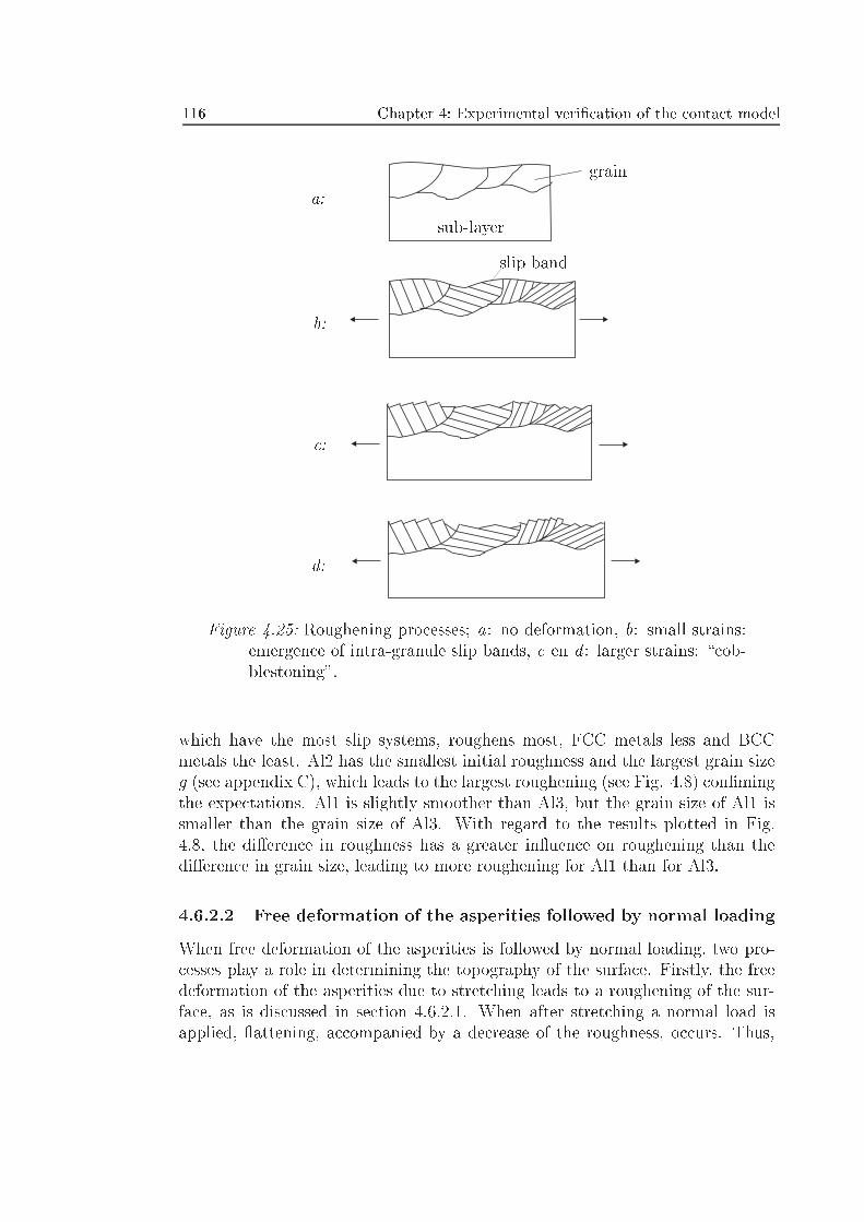
116 Chapter 4: Experimental veri�cation of the contact model
a:
b:
c:
d:
grain
sub-layer
slip band
Figure 4.25: Roughening processes; a: no deformation, b: small strains:emergence of intra-granule slip bands, c en d : larger strains: \cob-blestoning".
which have the most slip systems, roughens most, FCC metals less and BCCmetals the least. Al2 has the smallest initial roughness and the largest grain sizeg (see appendix C), which leads to the largest roughening (see Fig. 4.8) con�mingthe expectations. Al1 is slightly smoother than Al3, but the grain size of Al1 issmaller than the grain size of Al3. With regard to the results plotted in Fig.4.8, the di�erence in roughness has a greater in uence on roughening than thedi�erence in grain size, leading to more roughening for Al1 than for Al3.
4.6.2.2 Free deformation of the asperities followed by normal loading
When free deformation of the asperities is followed by normal loading, two pro-cesses play a role in determining the topography of the surface. Firstly, the freedeformation of the asperities due to stretching leads to a roughening of the sur-face, as is discussed in section 4.6.2.1. When after stretching a normal load isapplied, attening, accompanied by a decrease of the roughness, occurs. Thus,
4.7. Summary 117
a dynamic balance exists between the reduction of the surface heights due toapplication of the normal load and the increase of the surface heights due tounconstrained roughening. Whether an increase or a decrease of the roughnessoccurs, depends on which e�ect is stronger.
Fig. 4.11 shows that the real contact area is independent of the strain,implying that the hardness of the surface does not change during free deformationof the asperities. In contrast to simultaneous stretching and normal loadingexperiments, a decrease of the so-called \e�ective hardness", de�ned in section3.4.1.1, does not occur.
4.6.2.3 Deformation of asperities during simultaneous stretching andnormal loading
When a normal and a tensile force are applied simultaneously, the results dis-cussed in section 4.4.2.3, show that roughening and attening of a surface arecountervailing e�ects. For Al2 and Al3, the e�ect of roughening is strengthenedwhen a small nominal pressure is applied. Recently, similar results were reportedby Shih & Wilson (1999) for stretching and normal loading of a 0.92 mm thickMF 6022-T4 aluminium specimen.
Speci�c material properties are responsible for the enhanced roughening whena low nominal pressure is applied, because, in contrast to Al2 and Al3, Al1 hardlyshows an enhanced roughening e�ect. Possibly, as is the case in the normalloading experiments, the thickness of the material plays a role in the di�erences inbehaviour. When a normal and a tensile load are applied simultaneously, a thickmaterial may possibly cause an enhanced rotation of grains (\cobblestoning").For thin materials grains may be unable to rotate and attening dominates.However, this explanation is still speculative and further research is needed.
4.7 Summary
In this chapter experiments were described in which the theoretical contact modeldeveloped in chapter 3, was veri�ed. A special test device was developed, whichappears to be an adequate device for determining the topography of a surfaceduring application of a normal and/or a tension load. The experiments can beclassi�ed as static normal load experiments or stretching experiments, with orwithout normal loading.
Normal load experiments
� The static normal loading experiments show that the increase in the realcontact area is less than proportional to the load parameter P (pnom=H),which is in accordance with the model developed in chapter 3.
118 Chapter 4: Experimental veri�cation of the contact model
� Asperity persistence, the hardness and the thickness of the attened ma-terial, the nominal pressure and the asperity height distribution determinethe amount of attening.
� From the measured height distribution functions of the asperities, it can beconcluded that, due to application of a normal load, the valleys rise withan approximately constant value.
� Work hardening of the asperities, elastic deformation of the asperities andelastic recovery of the area beneath the indented asperities, play a minorrole during loading of a soft rough surface.
Equalling the asperity persistence parameter � to P (pnom=H), the ideal plasticcontact model predicts the real contact area rather well. The prediction can beimproved by making a correction for the in uence of the thickness of the materialby adapting the value of �. Substituting a value of � less than P in the contactmodel gives a better prediction of � for Al1 while a larger value of � leads to abetter prediction of � for Al2.
Stretching measurementsThree types of stretching measurements were performed.
� Free deformation. When a strip is stretched without application of a normalload, the surface of the strip roughens. It was found that the amount ofroughening is in uenced by the initial roughness of the surface and the grainsize. A smaller initial roughness and a larger grain size cause a greaterrelative roughening.
� Free deformation followed by normal loading. For this type of experiment,a dynamic balance between roughening, due to unconstrained stretching,and attening, due to the application of the normal load, determines theroughness of the tested surface. However, the fraction of real contact areais independent of the strain.
� Simultaneous stretching and normal loading. For Al1, the roughness be-comes less than the roughness found in the free deformation test. For highstrains, roughening increases. In the case of Al2 and Al3, it is found thatas long as the nominal pressure is lower than some critical value pcr, theroughness is greater than in the free deformation experiments. For largerpressures than pcr, the roughness decreases as a function of the nominalpressure. Performing these experiments, a dynamic balance between rough-ening and attening during stretching determines the overall e�ect on thetopography of a surface. The initial roughness, the grain size and probablythe thickness of the workpiece play a role in this process. The physical
4.7. Summary 119
mechanism(s), leading to an enhanced roughening when the nominal pres-sure is less than pcr, is (are) unknown.
For simultaneous stretching and normal loading, theoretical predictions weremade with the strain-contact model developed in section 3.4.2. Calculationswere performed for a plane strain and a plane stress deformation mode of theasperities. Fig. 4.18 shows a good agreement for Al1 between the predicted andexperimental results for both the plane stress as the plane strain situation. ForAl2 and AL3 the theoretical prediction is poor because the roughening behaviourof the surfaces of Al2 and Al3 is not included in the model.
Deep drawing experimentsDeep drawing experiments were performed to check the experimental results. Be-cause in deep drawing tests sliding occurs between the tools and the workpiece,one must be careful when comparing these results with the tensile tester results.However, it was found that the convex surface of the rectangular-hat-shaped cupsat the die rounding and the punch rounding regions roughen in a similar way as isfound for free deformation tests with the tensile tester. An estimation of the pres-sure peaks occurring at the concave surface of the cups at the die rounding andthe punch rounding regions was made, comparing the deep drawing results withthe tensile tester results in which simultaneous stretching and normal loading ofthe strip occurs.

120 Chapter 4: Experimental veri�cation of the contact model
Chapter 5
A macroscopic friction model
In chapter 2 expressions are given for the coeÆcient of friction in the case of slidingbetween a single hard asperity and a soft surface, which are both protected byboundary layers. In deep drawing operations, not one but many asperities on thetool are in contact with the workpiece. To predict friction during deep drawing,a macroscopic friction model is needed. This model will be derived here.
In the �rst section a number of friction models published in the literatureare discussed. In section 5.2 the structure of the newly developed friction modelis described. In section 5.3 the model is derived and the in uence of the mainparameters is discussed in section 5.4. The e�ect of the bulk strain on the frictionis treated in section 5.5. Finally, a summary is presented in section 5.6.
5.1 Overview of friction models
In this section a review is presented of the literature relating to macroscopicfriction models, which consider Boundary Lubrication and Ploughing (BL&P) ofhard asperities in contact with a soft material. When all hard asperities have thesame height and shape, the \attack angle" � of a ploughing hard asperity in a softmaterial (see section 2.4) is the same for all asperities. In this case the coeÆcientof friction for the macroscopic system can be simply obtained from eq. (2.18).However, in reality the hard asperities have di�erent heights, resulting in di�erent\attack angles", which makes a more sophisticated treatment necessary. Bassani,Di Pasquale & Vitali (1984) proposed a ploughing model to predict the frictionbetween an elastically deforming polymer and a rough metal surface. The RMS-roughness and the correlation length of the metal surface play a role in this model.Moalic, Fitzpatrick & Torrance (1987) applied the model of Challen & Oxley(1979), discussed in section 2.4, for modelling the contact between a soft surfaceand a hard surface with � determined by means of a �nite Fourier transform ofthe heights of the surface. Zhang, Moslehy & Rice (1991) developed a friction
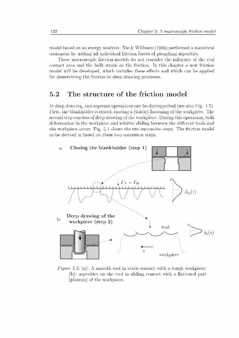
122 Chapter 5: A macroscopic friction model
model based on an energy analysis. Xie & Williams (1996) performed a statisticaltreatment by adding all individual friction forces of ploughing asperities.
These macroscopic friction models do not consider the in uence of the realcontact area and the bulk strain on the friction. In this chapter a new frictionmodel will be developed, which includes these e�ects and which can be appliedfor determining the friction in deep drawing processes.
5.2 The structure of the friction model
In deep drawing, two seperate operations can be distinguished (see also Fig. 1.2).First, the blankholder is closed, causing a (static) attening of the workpiece. Thesecond step consists of deep drawing of the workpiece. During this operation, bulkdeformation in the workpiece and relative sliding between the di�erent tools andthe workpiece occur. Fig. 5.1 shows the two successive steps. The friction modelto be derived is based on these two successive steps.
�w(z)
zFN = Fbl
�t(s)
s
Closing the blankholder (step 1)
Deep drawing of theworkpiece (step 2)
a:
b:
vworkpiece
tool
Figure 5.1: (a): A smooth tool in static contact with a rough workpiece;(b): asperities on the tool in sliding contact with a attened part(plateau) of the workpiece.
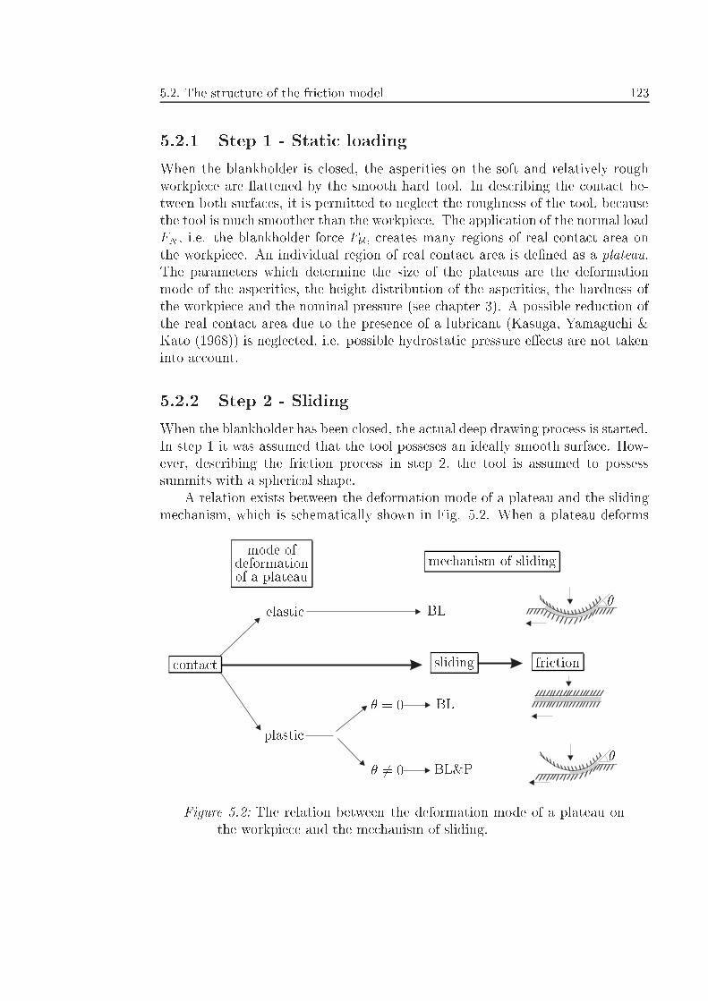
5.2. The structure of the friction model 123
5.2.1 Step 1 - Static loading
When the blankholder is closed, the asperities on the soft and relatively roughworkpiece are attened by the smooth hard tool. In describing the contact be-tween both surfaces, it is permitted to neglect the roughness of the tool, becausethe tool is much smoother than the workpiece. The application of the normal loadFN , i.e. the blankholder force Fbl, creates many regions of real contact area onthe workpiece. An individual region of real contact area is de�ned as a plateau.The parameters which determine the size of the plateaus are the deformationmode of the asperities, the height distribution of the asperities, the hardness ofthe workpiece and the nominal pressure (see chapter 3). A possible reduction ofthe real contact area due to the presence of a lubricant (Kasuga, Yamaguchi &Kato (1968)) is neglected, i.e. possible hydrostatic pressure e�ects are not takeninto account.
5.2.2 Step 2 - Sliding
When the blankholder has been closed, the actual deep drawing process is started.In step 1 it was assumed that the tool posseses an ideally smooth surface. How-ever, describing the friction process in step 2, the tool is assumed to possesssummits with a spherical shape.
A relation exists between the deformation mode of a plateau and the slidingmechanism, which is schematically shown in Fig. 5.2. When a plateau deforms
mode ofdeformationof a plateau
contact
elastic
plastic
sliding friction
� = 0
� 6= 0
BL
BL
BL&P
mechanism of sliding
�
�
Figure 5.2: The relation between the deformation mode of a plateau onthe workpiece and the mechanism of sliding.
124 Chapter 5: A macroscopic friction model
completely elastically, energy losses due to ploughing do not occur. Only BL oc-curs and the friction is due to shear of boundary layers. For plastically deformingplateaus friction is always due to a combined action of BL and ploughing. Theonly exception would be a perfectly smooth tool (� = 0). Theoretically, whenthe tool is perfectly smooth, shear in the boundary layer (BL) occurs, which isindependent of the deformation mode of the plateau. However, this situation isonly theoretical, because in reality every surface possesses a roughness.
5.3 The model
5.3.1 Assumptions
In deriving the friction model, the following assumptions are made:
� Application of the normal load is followed by sliding.
� The in uence of the sliding speed is neglected.
� No dry contact occurs between the tool and the workpiece.
� No solidi�cation of the lubricant occurs.
� The temperature is assumed to be constant.
� There is no e�ect of the workpiece material, i.e. no roughening e�ect andno e�ects of oxide layers and coatings.
� There is no e�ect of the tool material.
These assumptions will be discussed in some detail.
Sliding contactThe friction model is based on two steps. Firstly, the workpiece is considered tobe attened by a smooth at tool, followed by sliding between the tool and theworkpiece and eventually stretching of the workpiece. In fact, this way of calcu-lating the friction may not be applied when contact between the workpiece andthe tool occurs when deep drawing has already started (i.e., �rst sliding, followedby application of a normal force). This happens for example in the die roundingand the stamp rounding region. However, as long as the e�ect of sliding on thereal contact area can be neglected, which is usually allowed in well lubricatedcontacts, this way of calculating the friction also applies for \fresh" workpiecematerial which comes in contact with the tool.
5.3. The model 125
Dry contactIn the model it is assumed that the surfaces of the tool and the workpiece are to-tally protected by a boundary �lm. The possible occurrence of local dry contactcan be incorporated in the model as follows. As proposed by Torrance (1997),a fraction d can be de�ned as the fraction of the contact area which is notprotected by bounday layers. In this case, the friction factor fC can be writtenas:
fC =�BL(1� d) + k d
k= 3p3(1� d)fBL + d (5.1)
with 0 � d � 1. Unfortunately, values of d cannot be determined directly. Dueto the part of the surface which is not protected by boundary layers, the frictionforce will increase, compared to the case of a complete coverage of boundary lay-ers.
Solid layersInstead of BL, the contact between the tool and the workpiece may be (locally)lubricated by solid layers. In that case the friction of the lubricant �lm is nolonger caused by shear of adsorbed boundary layers, but by shear of thin solidlayers, which may form under conditions of local high pressures (i.e. the hardness)and smooth surfaces (the attened plateaus). A transition of the lubricant fromthe liquid to the solid phase has been demonstrated by Bair & Winer (1982) andSchipper (1988). Studies of solid behaviour of lubricants, based on a molecularscale, have been performed by Gee, McGuiggan, Israelachvili & Homola (1990)and Granick (1991). The shear strength of solid layers is called the limiting shearstrength. For Shell Vitrea 79 and the traction uid Santotrac 50 it was shown byBlack et al. (1990) that the shear stress of the boundary �lm was indeed the limit-ing shear strength when a soft surface was moved along a hard wedge shaped tool.
TemperatureIn section 2.2.2.3 it was shown that for di�erent types of acid boundary layers,the friction decreases for increasing temperatures. Because deep drawing gen-erally happens at a constant temperature, no attention is paid to the e�ect oftemperature on friction.
Workpiece materialIn the model, the in uence of the type of workpiece material on the friction is nottaken into account. For example, roughening e�ects due to simultaneous normalloading and bulk stretching (see section 4.4.2.3) are not included in calculationsof the e�ect of the strain on the friction. When roughening of the workpieceoccurs, the real contact area decreases as a function of the strain. This e�ectimplies that the coeÆcient of friction decreases as a function of the strain, which
126 Chapter 5: A macroscopic friction model
is the opposite e�ect of the results obtained in section 5.5. Measurements bySaha & Wilson (1994) con�rm this e�ect, �nding an increasing friction for steeland a decreasing friction for aluminium as a function of the strain.
Another possible in uence of the workpiece material, which is not includedin the friction model, is the e�ect of solid surface layers on the friction, as, forexample, oxide layers and coatings. For example, depositing stearic acid layerson an aluminium coated mica substrate, gives a higher friction than when stearicacid is directly adsorbed onto mica (Timsit & Pelow (1992b).
Tool materialThe e�ect of the tool material on the friction is not considered here. A possiblee�ect of a di�erent tool material may be the in uence on the shear strength ofadsorbed boundary layers.
5.3.2 Step 1 - static loading
From now on, elastic deformation of the workpiece asperities is neglected. Whenthe workpiece is normally loaded by the tool, it is assumed that the asperities onthe workpiece deform ideal plastically. Therefore, eqs. (3.44), (3.50) and (3.51)can be solved simultaneously to obtain the fraction of real contact area �, i.e.,the total real contact area of the plateaus divided by the nominal contact area.It can be concluded from chapter 4 that � = P and n = 1 are realistic values of,respectively, the asperity persistence parameter � and the indentation parametern. In addition to these parameters, the nominal pressure, the hardness of theworkpiece and the height distribution function of the workpiece asperities �w(z)are needed to determine the amount of attening.
5.3.3 Step 2 - sliding
In order to describe the friction during deep drawing, the tool is assumed to berough. The radius of the spherical summits �t of the tool is assumed to be thesame for all summits. �t is the areal density of the summits, i.e., the number ofsummits per unit area. A new separation Æ is de�ned as the distance betweenthe mean plane of the tool summits and the at plateaus of the workpiece. Be-cause the whole plateau is in contact with the tool (a result of step 1), Æ can bedetermined from the condition:Z smax
Æ
�t(s)ds = 1 (5.2)
�t(s) is the height distribution function of the summits on the tool and smax isthe maximum height of the summits. From eq. (5.2) it follows that
Æ = smin (5.3)
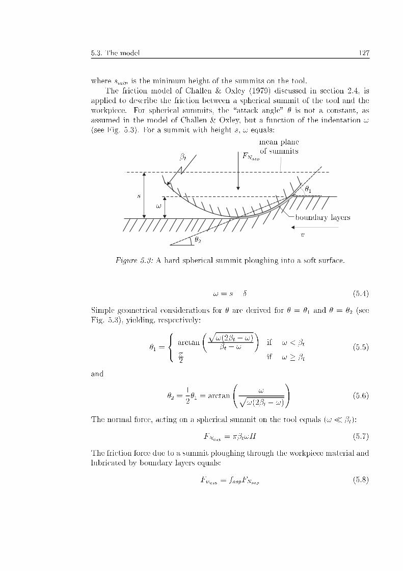
5.3. The model 127
where smin is the minimum height of the summits on the tool.The friction model of Challen & Oxley (1979) discussed in section 2.4, is
applied to describe the friction between a spherical summit of the tool and theworkpiece. For spherical summits, the \attack angle" � is not a constant, asassumed in the model of Challen & Oxley, but a function of the indentation !(see Fig. 5.3). For a summit with height s, ! equals:
!
v
�t FNasp
�1
�2
boundary layers
s
mean planeof summits
Figure 5.3: A hard spherical summit ploughing into a soft surface.
! = s� Æ (5.4)
Simple geometrical considerations for � are derived for � = �1 and � = �2 (seeFig. 5.3), yielding, respectively:
�1 =
8<: arctan
�p!(2�t � !)�t � !
�if ! < �t
�2 if ! � �t
(5.5)
and
�2 =1
2�1 = arctan
!p
!(2�t � !)
!(5.6)
The normal force, acting on a spherical summit on the tool equals (! � �t):
FNasp = ��t!H (5.7)
The friction force due to a summit ploughing through the workpiece material andlubricated by boundary layers equals:
Fwasp = faspFNasp (5.8)
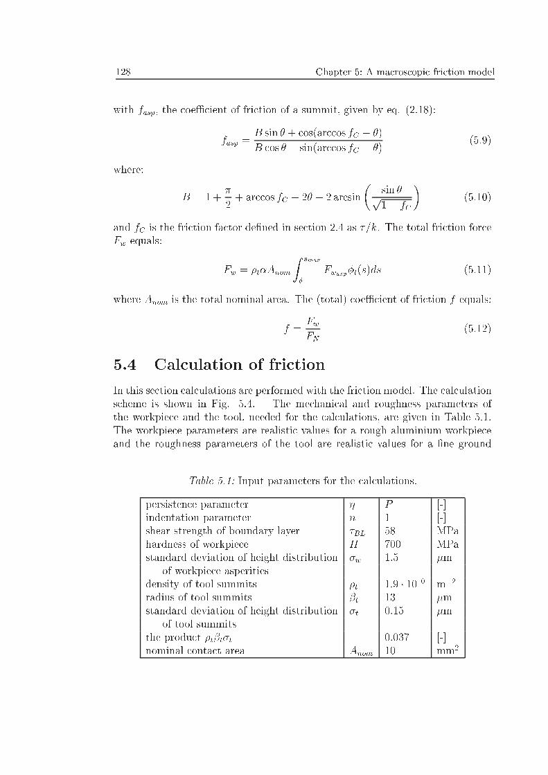
128 Chapter 5: A macroscopic friction model
with fasp, the coeÆcient of friction of a summit, given by eq. (2.18):
fasp =B sin � + cos(arccos fC � �)
B cos � + sin(arccos fC � �)(5.9)
where:
B = 1 +�
2+ arccos fC � 2� � 2 arcsin
�sin �p1� fC
�(5.10)
and fC is the friction factor de�ned in section 2.4 as �=k. The total friction forceFw equals:
Fw = �t�Anom
Z smax
Æ
Fwasp�t(s)ds (5.11)
where Anom is the total nominal area. The (total) coeÆcient of friction f equals:
f =FwFN
(5.12)
5.4 Calculation of friction
In this section calculations are performed with the friction model. The calculationscheme is shown in Fig. 5.4. The mechanical and roughness parameters ofthe workpiece and the tool, needed for the calculations, are given in Table 5.1.The workpiece parameters are realistic values for a rough aluminium workpieceand the roughness parameters of the tool are realistic values for a �ne ground
Table 5.1: Input parameters for the calculations.
persistence parameter � P [-]indentation parameter n 1 [-]shear strength of boundary layer �BL 58 MPahardness of workpiece H 700 MPastandard deviation of height distribution �w 1.5 �m
of workpiece asperitiesdensity of tool summits �t 1:9 � 1010 m�2
radius of tool summits �t 13 �mstandard deviation of height distribution �t 0.15 �m
of tool summitsthe product �t�t�t 0.037 [-]nominal contact area Anom 10 mm2
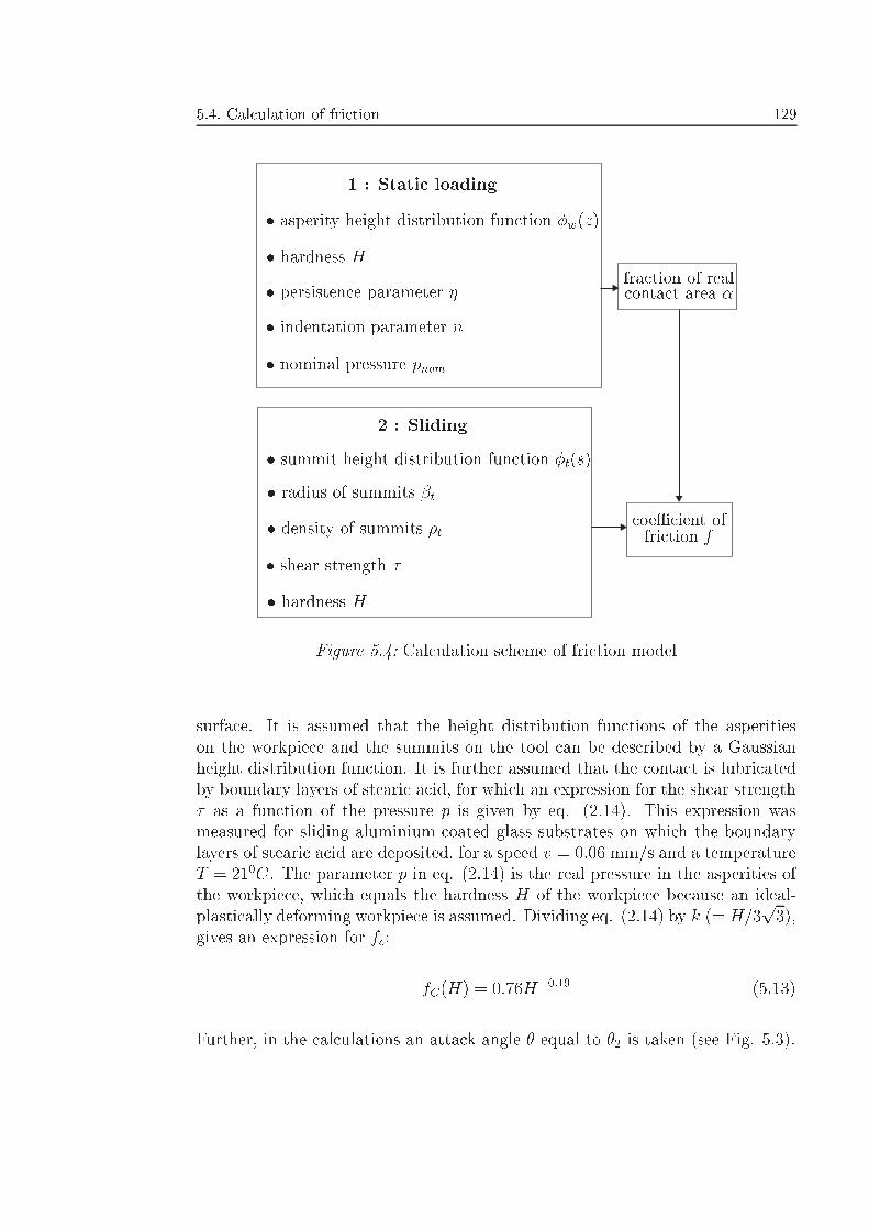
5.4. Calculation of friction 129
1 : Static loading
2 : Sliding
� asperity height distribution function �w(z)
� hardness H� persistence parameter �
� indentation parameter n
� nominal pressure pnom
fraction of realcontact area �
� summit height distribution function �t(s)
� radius of summits �t
� density of summits �t
� shear strength �� hardness H
coeÆcient offriction f
Figure 5.4: Calculation scheme of friction model
surface. It is assumed that the height distribution functions of the asperitieson the workpiece and the summits on the tool can be described by a Gaussianheight distribution function. It is further assumed that the contact is lubricatedby boundary layers of stearic acid, for which an expression for the shear strength� as a function of the pressure p is given by eq. (2.14). This expression wasmeasured for sliding aluminium coated glass substrates on which the boundarylayers of stearic acid are deposited, for a speed v = 0:06 mm/s and a temperatureT = 210C. The parameter p in eq. (2.14) is the real pressure in the asperities ofthe workpiece, which equals the hardness H of the workpiece because an ideal-plastically deforming workpiece is assumed. Dividing eq. (2.14) by k (= H=3
p3),
gives an expression for fc:
fC(H) = 0:76H�0:19 (5.13)
Further, in the calculations an attack angle � equal to �2 is taken (see Fig. 5.3).
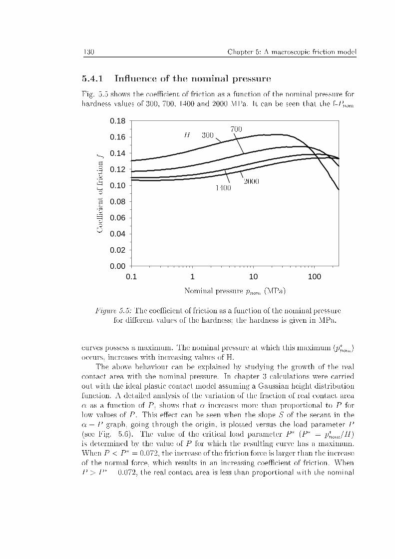
130 Chapter 5: A macroscopic friction model
5.4.1 In uence of the nominal pressure
Fig. 5.5 shows the coeÆcient of friction as a function of the nominal pressure forhardness values of 300, 700, 1400 and 2000 MPa. It can be seen that the f-Pnom
0.1 1 10 1000.00
0.02
0.04
0.06
0.08
0.10
0.12
0.14
0.16
0.18
Nominal pressure pnom (MPa)
CoeÆcientoffrictionf
H = 300700
14002000
Figure 5.5: The coeÆcient of friction as a function of the nominal pressurefor di�erent values of the hardness; the hardness is given in MPa.
curves possess a maximum. The nominal pressure at which this maximum (p�nom)occurs, increases with increasing values of H.
The above behaviour can be explained by studying the growth of the realcontact area with the nominal pressure. In chapter 3 calculations were carriedout with the ideal plastic contact model assuming a Gaussian height distributionfunction. A detailed analysis of the variation of the fraction of real contact area� as a function of P , shows that � increases more than proportional to P forlow values of P . This e�ect can be seen when the slope S of the secant in the� � P graph, going through the origin, is plotted versus the load parameter P(see Fig. 5.6). The value of the critical load parameter P � (P � = p�nom=H)is determined by the value of P for which the resulting curve has a maximum.When P < P � = 0:072, the increase of the friction force is larger than the increaseof the normal force, which results in an increasing coeÆcient of friction. WhenP > P � = 0:072, the real contact area is less than proportional with the nominal
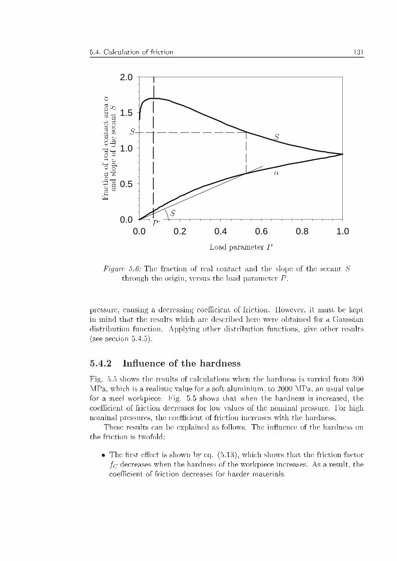
5.4. Calculation of friction 131
0.0 0.2 0.4 0.6 0.8 1.00.0
0.5
1.0
1.5
2.0
Load parameter P
Fr ac ti onofrealcont acta re a�
andslo peoft hesecantS
�
S
P �
S
S
Figure 5.6: The fraction of real contact and the slope of the secant Sthrough the origin, versus the load parameter P .
pressure, causing a decreasing coeÆcient of friction. However, it must be keptin mind that the results which are described here were obtained for a Gaussiandistribution function. Applying other distribution functions, give other results(see section 5.4.5).
5.4.2 In uence of the hardness
Fig. 5.5 shows the results of calculations when the hardness is varried from 300MPa, which is a realistic value for a soft aluminium, to 2000 MPa, an usual valuefor a steel workpiece. Fig. 5.5 shows that when the hardness is increased, thecoeÆcient of friction decreases for low values of the nominal pressure. For highnominal pressures, the coeÆcient of friction increases with the hardness.
These results can be explained as follows. The in uence of the hardness onthe friction is twofold:
� The �rst e�ect is shown by eq. (5.13), which shows that the friction factorfC decreases when the hardness of the workpiece increases. As a result, thecoeÆcient of friction decreases for harder materials.
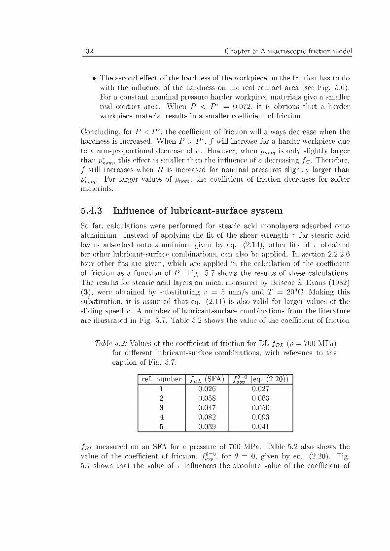
132 Chapter 5: A macroscopic friction model
� The second e�ect of the hardness of the workpiece on the friction has to dowith the in uence of the hardness on the real contact area (see Fig. 5.6).For a constant nominal pressure harder workpiece materials give a smallerreal contact area. When P < P � = 0:072, it is obvious that a harderworkpiece material results in a smaller coeÆcient of friction.
Concluding, for P < P �, the coeÆcient of friction will always decrease when thehardness is increased. When P > P �, f will increase for a harder workpiece dueto a non-proportional decrease of �. However, when pnom is only slightly largerthan p�nom, this e�ect is smaller than the in uence of a decreasing fC . Therefore,f still increases when H is increased for nominal pressures slightly larger thanp�nom. For larger values of pnom, the coeÆcient of friction decreases for softermaterials.
5.4.3 In uence of lubricant-surface system
So far, calculations were performed for stearic acid monolayers adsorbed ontoaluminium. Instead of applying the �t of the shear strength � for stearic acidlayers adsorbed onto aluminium given by eq. (2.14), other �ts of � obtainedfor other lubricant-surface combinations, can also be applied. In section 2.2.2.6four other �ts are given, which are applied in the calculation of the coeÆcientof friction as a function of P . Fig. 5.7 shows the results of these calculations.The results for stearic acid layers on mica, measured by Briscoe & Evans (1982)(3), were obtained by substituting v = 5 mm/s and T = 200C. Making thissubstitution, it is assumed that eq. (2.11) is also valid for larger values of thesliding speed v. A number of lubricant-surface combinations from the literatureare illustrated in Fig. 5.7. Table 5.2 shows the value of the coeÆcient of friction
Table 5.2: Values of the coeÆcient of friction for BL fBL (p = 700 MPa)for di�erent lubricant-surface combinations, with reference to thecaption of Fig. 5.7.
ref. number fBL (SFA) f �=0asp (eq. (2.20))1 0.026 0.0272 0.058 0.0633 0.047 0.0504 0.082 0.0935 0.039 0.041
fBL measured on an SFA for a pressure of 700 MPa. Table 5.2 also shows thevalue of the coeÆcient of friction, f �=0asp , for � = 0, given by eq. (2.20). Fig.5.7 shows that the value of � in uences the absolute value of the coeÆcient of
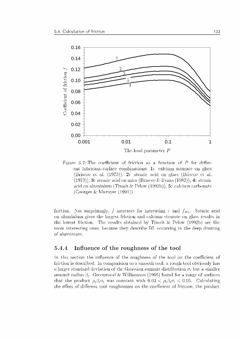
5.4. Calculation of friction 133
0.001 0.01 0.1 10.00
0.02
0.04
0.06
0.08
0.10
0.12
0.14
0.16
The load parameter P
CoeÆcientoff ri ctionf
1
23
4
5
Figure 5.7: The coeÆcient of friction as a function of P for di�er-ent lubricant-surface combinations; 1: calcium stearate on glass(Briscoe et al. (1973)), 2: stearic acid on glass (Briscoe et al.(1973)), 3: stearic acid on mica (Briscoe & Evans (1982)), 4: stearicacid on aluminium (Timsit & Pelow (1992b)), 5: calcium carbonate(Georges & Mazuyer (1991)).
friction. Not surprisingly, f increases for increasing � and fBL. Stearic acidon aluminium gives the largest friction and calcium stearate on glass results inthe lowest friction. The results obtained by Timsit & Pelow (1992b) are themost interesting ones, because they describe BL occurring in the deep drawingof aluminium.
5.4.4 In uence of the roughness of the tool
In this section the in uence of the roughness of the tool on the coeÆcient offriction is described. In comparision to a smooth tool, a rough tool obviously hasa larger standard deviation of the Gaussian summit distribution �t but a smallersummit radius �t. Greenwood & Williamson (1966) found for a range of surfacesthat the product �t�t�t was constant with 0:03 < �t�t�t < 0:05. Calculatingthe e�ect of di�erent tool roughnesses on the coeÆcient of friction, the product
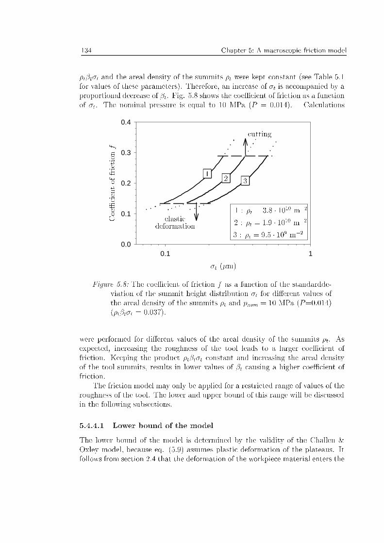
134 Chapter 5: A macroscopic friction model
�t�t�t and the areal density of the summits �t were kept constant (see Table 5.1for values of these parameters). Therefore, an increase of �t is accompanied by aproportional decrease of �t. Fig. 5.8 shows the coeÆcient of friction as a functionof �t. The nominal pressure is equal to 10 MPa (P = 0.014). Calculations
0.1 10.0
0.1
0.2
0.3
0.4
�t (�m)
CoeÆcientoffrictio nf
cutting
elasticdeformation
12 3
3 : �t = 9:5 � 109 m�2
2 : �t = 1:9 � 1010 m�2
1 : �t = 3:8 � 1010 m�2
Figure 5.8: The coeÆcient of friction f as a function of the standardde-viation of the summit height distribution �t for di�erent values ofthe areal density of the summits �t and pnom = 10 MPa (P=0.014)(�t�t�t = 0.037).
were performed for di�erent values of the areal density of the summits �t. Asexpected, increasing the roughness of the tool leads to a larger coeÆcient offriction. Keeping the product �t�t�t constant and increasing the areal densityof the tool summits, results in lower values of �t causing a higher coeÆcient offriction.
The friction model may only be applied for a restricted range of values of theroughness of the tool. The lower and upper bound of this range will be discussedin the following subsections.
5.4.4.1 Lower bound of the model
The lower bound of the model is determined by the validity of the Challen &Oxley model, because eq. (5.9) assumes plastic deformation of the plateaus. Itfollows from section 2.4 that the deformation of the workpiece material enters the
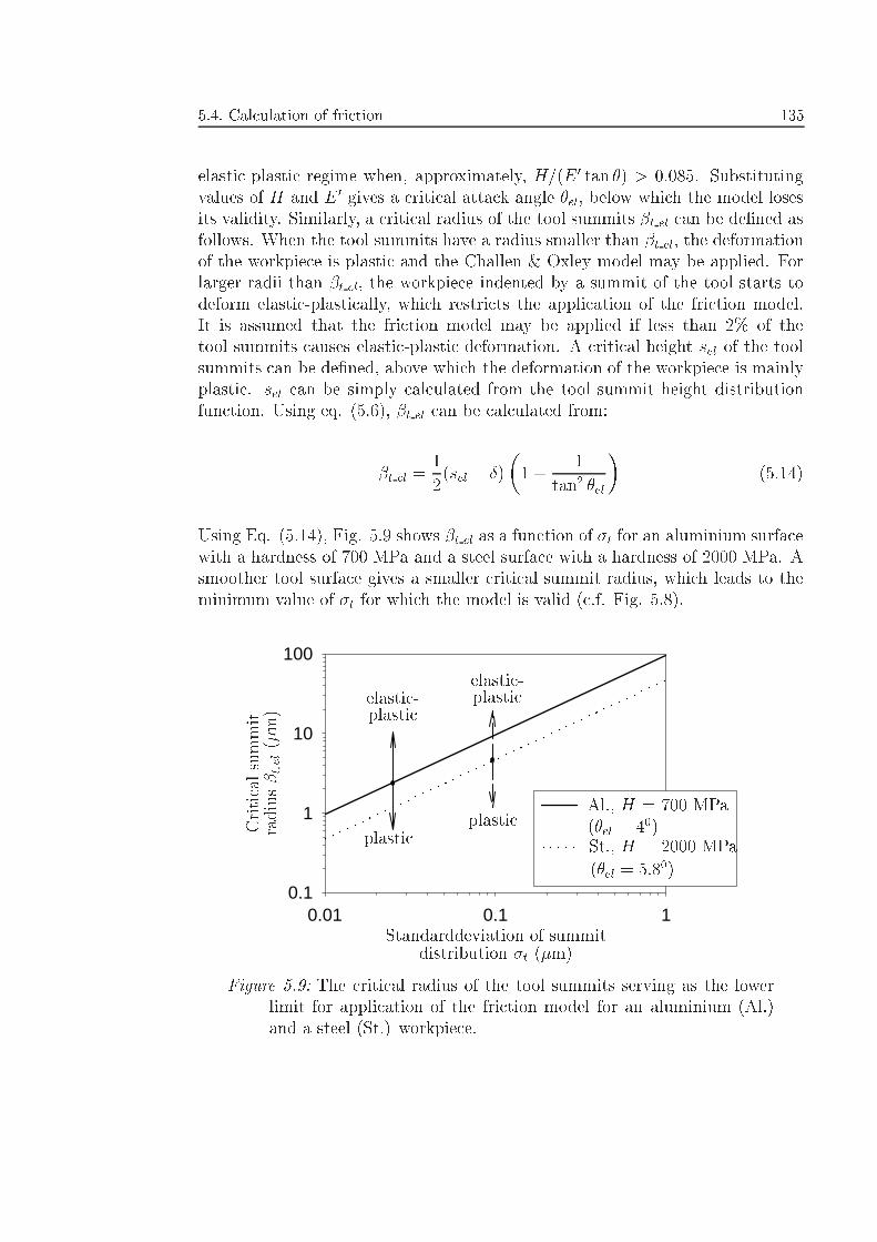
5.4. Calculation of friction 135
elastic-plastic regime when, approximately, H=(E 0 tan �) > 0:085. Substitutingvalues of H and E 0 gives a critical attack angle �el, below which the model losesits validity. Similarly, a critical radius of the tool summits �t el can be de�ned asfollows. When the tool summits have a radius smaller than �t el, the deformationof the workpiece is plastic and the Challen & Oxley model may be applied. Forlarger radii than �t el, the workpiece indented by a summit of the tool starts todeform elastic-plastically, which restricts the application of the friction model.It is assumed that the friction model may be applied if less than 2% of thetool summits causes elastic-plastic deformation. A critical height sel of the toolsummits can be de�ned, above which the deformation of the workpiece is mainlyplastic. sel can be simply calculated from the tool summit height distributionfunction. Using eq. (5.6), �t el can be calculated from:
�t el =1
2(sel � Æ)
�1 +
1
tan2 �el
�(5.14)
Using Eq. (5.14), Fig. 5.9 shows �t el as a function of �t for an aluminium surfacewith a hardness of 700 MPa and a steel surface with a hardness of 2000 MPa. Asmoother tool surface gives a smaller critical summit radius, which leads to theminimum value of �t for which the model is valid (c.f. Fig. 5.8).
0.01 0.1 10.1
1
10
100
Standarddeviation of summitdistribution �t (�m)
Criticalsummit
radi us�tel(�m)
elastic-plasticelastic-
plastic
plasticplastic
Al., H = 700 MPa(�el = 40)St., H = 2000 MPa
(�el = 5:80)
Figure 5.9: The critical radius of the tool summits serving as the lowerlimit for application of the friction model for an aluminium (Al.)and a steel (St.) workpiece.
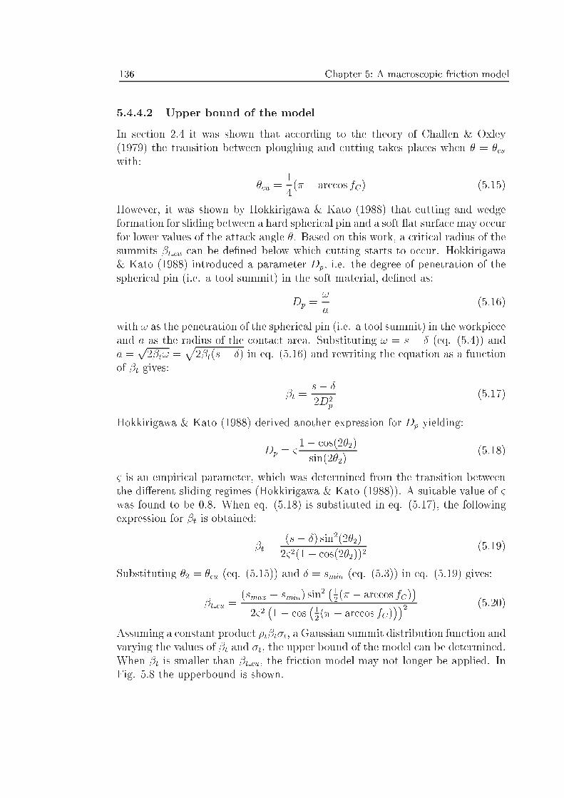
136 Chapter 5: A macroscopic friction model
5.4.4.2 Upper bound of the model
In section 2.4 it was shown that according to the theory of Challen & Oxley(1979) the transition between ploughing and cutting takes places when � = �cuwith:
�cu =1
4(� � arccos fC) (5.15)
However, it was shown by Hokkirigawa & Kato (1988) that cutting and wedgeformation for sliding between a hard spherical pin and a soft at surface may occurfor lower values of the attack angle �. Based on this work, a critical radius of thesummits �t cu can be de�ned below which cutting starts to occur. Hokkirigawa& Kato (1988) introduced a parameter Dp, i.e. the degree of penetration of thespherical pin (i.e. a tool summit) in the soft material, de�ned as:
Dp =!
a(5.16)
with ! as the penetration of the spherical pin (i.e. a tool summit) in the workpieceand a as the radius of the contact area. Substituting ! = s � Æ (eq. (5.4)) anda =
p2�t! =
p2�t(s� Æ) in eq. (5.16) and rewriting the equation as a function
of �t gives:
�t =s� Æ
2D2p
(5.17)
Hokkirigawa & Kato (1988) derived another expression for Dp yielding:
Dp = &1� cos(2�2)
sin(2�2)(5.18)
& is an empirical parameter, which was determined from the transition betweenthe di�erent sliding regimes (Hokkirigawa & Kato (1988)). A suitable value of &was found to be 0.8. When eq. (5.18) is substituted in eq. (5.17), the followingexpression for �t is obtained:
�t =(s� Æ) sin2(2�2)
2&2(1� cos(2�2))2(5.19)
Substituting �2 = �cu (eq. (5.15)) and Æ = smin (eq. (5.3)) in eq. (5.19) gives:
�t cu =(smax � smin) sin
2�1
2(� � arccos fC)
�2&2�1� cos
�1
2(� � arccos fC)
��2 (5.20)
Assuming a constant product �t�t�t, a Gaussian summit distribution function andvarying the values of �t and �t, the upper bound of the model can be determined.When �t is smaller than �t cu, the friction model may not longer be applied. InFig. 5.8 the upperbound is shown.
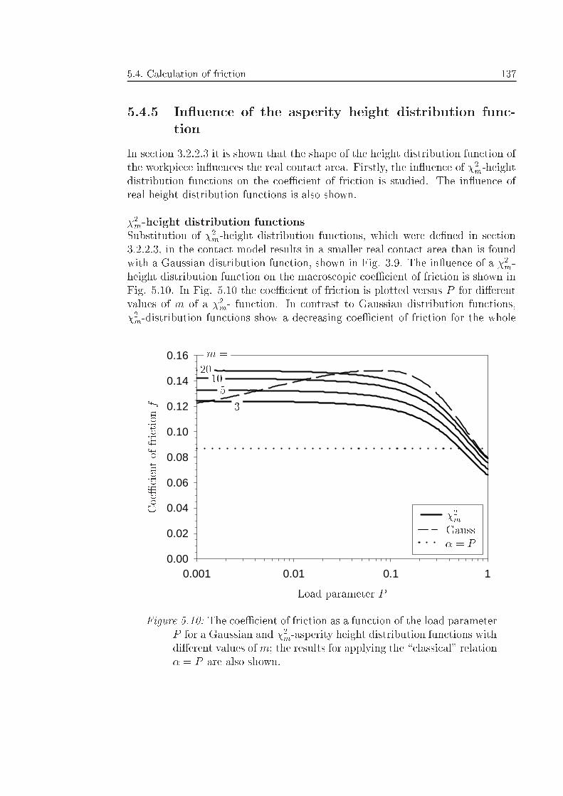
5.4. Calculation of friction 137
5.4.5 In uence of the asperity height distribution func-tion
In section 3.2.2.3 it is shown that the shape of the height distribution function ofthe workpiece in uences the real contact area. Firstly, the in uence of �2m-heightdistribution functions on the coeÆcient of friction is studied. The in uence ofreal height distribution functions is also shown.
�2m-height distribution functionsSubstitution of �2m-height distribution functions, which were de�ned in section3.2.2.3, in the contact model results in a smaller real contact area than is foundwith a Gaussian distribution function, shown in Fig. 3.9. The in uence of a �2m-height distribution function on the macroscopic coeÆcient of friction is shown inFig. 5.10. In Fig. 5.10 the coeÆcient of friction is plotted versus P for di�erentvalues of m of a �2m- function. In contrast to Gaussian distribution functions,�2m-distribution functions show a decreasing coeÆcient of friction for the whole
0.001 0.01 0.1 10.00
0.02
0.04
0.06
0.08
0.10
0.12
0.14
0.16
Load parameter P
CoeÆcie ntoffrict io nf
� = PGauss
20105
3
m =
�2m
Figure 5.10: The coeÆcient of friction as a function of the load parameterP for a Gaussian and �2m-asperity height distribution functions withdi�erent values ofm; the results for applying the \classical" relation� = P are also shown.
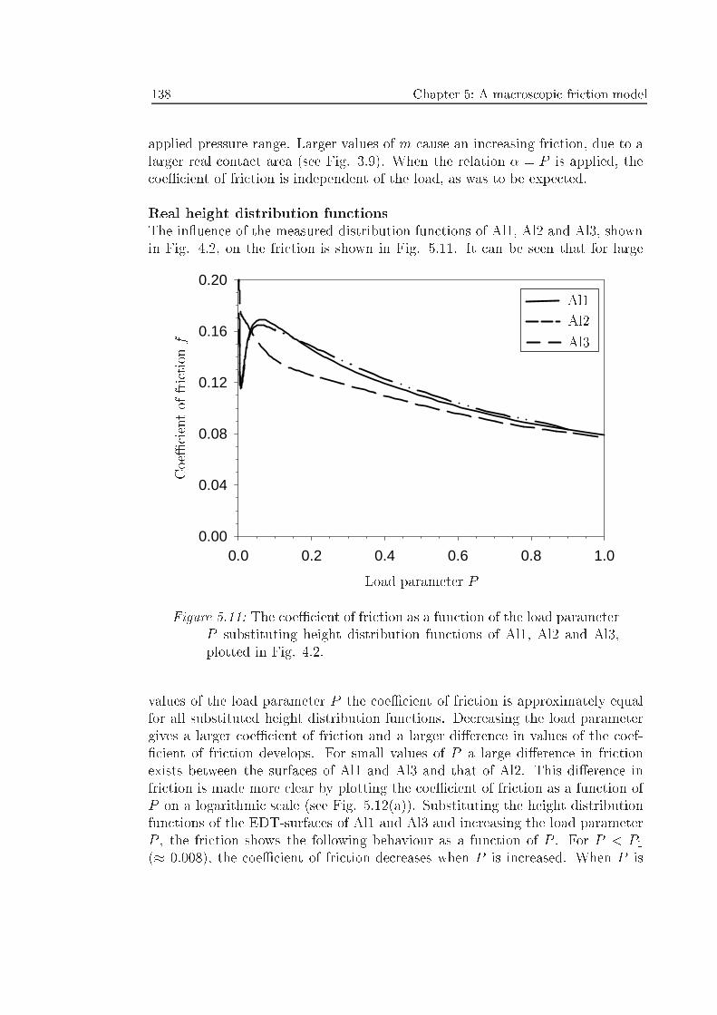
138 Chapter 5: A macroscopic friction model
applied pressure range. Larger values of m cause an increasing friction, due to alarger real contact area (see Fig. 3.9). When the relation � = P is applied, thecoeÆcient of friction is independent of the load, as was to be expected.
Real height distribution functionsThe in uence of the measured distribution functions of Al1, Al2 and Al3, shownin Fig. 4.2, on the friction is shown in Fig. 5.11. It can be seen that for large
0.0 0.2 0.4 0.6 0.8 1.00.00
0.04
0.08
0.12
0.16
0.20
Load parameter P
CoeÆcie ntoffrict io nf
Al1
Al2
Al3
Figure 5.11: The coeÆcient of friction as a function of the load parameterP substituting height distribution functions of Al1, Al2 and Al3,plotted in Fig. 4.2.
values of the load parameter P the coeÆcient of friction is approximately equalfor all substituted height distribution functions. Decreasing the load parametergives a larger coeÆcient of friction and a larger di�erence in values of the coef-�cient of friction develops. For small values of P a large di�erence in frictionexists between the surfaces of Al1 and Al3 and that of Al2. This di�erence infriction is made more clear by plotting the coeÆcient of friction as a function ofP on a logarithmic scale (see Fig. 5.12(a)). Substituting the height distributionfunctions of the EDT-surfaces of Al1 and Al3 and increasing the load parameterP , the friction shows the following behaviour as a function of P . For P < P1(� 0:008), the coeÆcient of friction decreases when P is increased. When P is
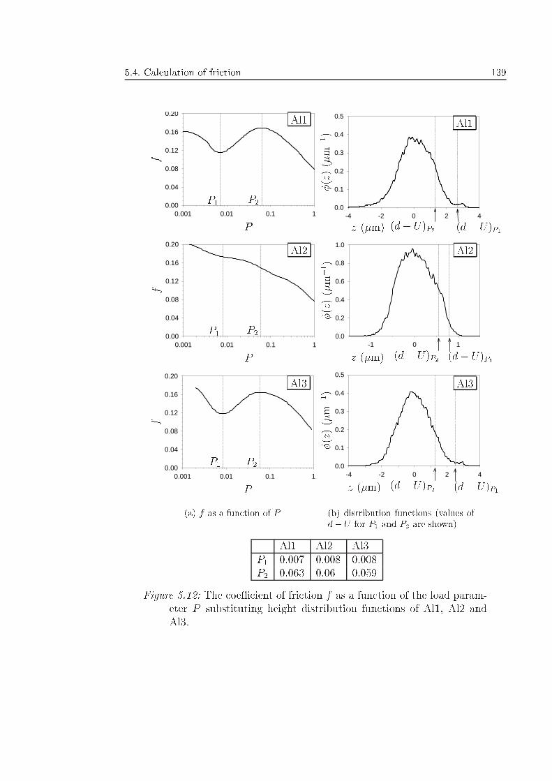
5.4. Calculation of friction 139
0.001 0.01 0.1 10.00
0.04
0.08
0.12
0.16
0.20
0.001 0.01 0.1 10.00
0.04
0.08
0.12
0.16
0.20
0.001 0.01 0.1 10.00
0.04
0.08
0.12
0.16
0.20
P
P
P
f
f
f
Al1
Al2
Al3
P1
P1
P1
P2
P2
P2
(a) f as a function of P
-4 -2 0 2 40.0
0.1
0.2
0.3
0.4
0.5
-1 0 10.0
0.2
0.4
0.6
0.8
1.0
-4 -2 0 2 40.0
0.1
0.2
0.3
0.4
0.5
z (�m)
z (�m)
z (�m)
�(z)(�m�1)
�( z)( �m�1)
�(z)(�m�1)
Al1
Al2
Al3
(d� U)P1
(d� U)P1
(d� U)P1
(d� U)P2
(d� U)P2
(d� U)P2
(b) distribution functions (values ofd� U for P1 and P2 are shown)
Al1 Al2 Al3P1 0.007 0.008 0.008P2 0.063 0.06 0.059
Figure 5.12: The coeÆcient of friction f as a function of the load param-eter P substituting height distribution functions of Al1, Al2 andAl3.
140 Chapter 5: A macroscopic friction model
increased from P1 (� 0:008) to P2 (� 0:06), the coeÆcient of friction increases.For larger values of P than P2, the friction decreases for increasing values of P .On the other hand, when the distribution function of the MF-surface of Al2 issubstituted in the friction model, a steadily decreasing coeÆcient of friction isfound for all values of P .
The reason for the di�erence in friction behaviour between the EDT-surfaces(Al1 and Al3) and the MF-surface (Al2), lies in the di�erence in surface heightdistribution. In Fig. 5.12(b) the three measured asperity height distributionfunctions of Al1, Al2 and Al3 are shown. In Fig. 5.12(b) the values of d � U ,i.e. the lower limits of the integration of �(z) for determining �, for P = P1and P = P2 are shown. Although for Al2 values of P1 and P2 cannot be given,corresponding values of d � U for P = 0:008 and P = 0:06 are given for refer-ence. It is obvious that the distribution of the highest asperities of the surfacesstrongly in uences the amount of attening for low values of the load parameterP and, therefore, the coeÆcient of friction. The distribution function of Al2 isrelatively regular, which causes a steadily decreasing coeÆcient of friction whenthe load is increased. On the other hand, the EDT surfaces Al1 and Al3 show anirregular distribution for the highest asperities, causing the above dependence ofthe coeÆcient of friction as a function of P .
5.5 In uence of the bulk strain
In the previous section calculations of the coeÆcient of friction were performed,assuming a normal load only. However, in deep drawing proceses the workpiece issimultaneously stretched and normally loaded at the die rouding and the punchrounding regions. In chapters 3 and 4 it was shown that simultaneous stretchingand normal loading largely in uences the real contact area of the workpiece and,therefore, the friction.
Assuming an ideal-plastically deforming workpiece, which is simultaneouslystretched and normally loaded, the real contact area can be calculated using thecontact-strain model, derived in section 3.4.2. The roughening of the workpiece,which is measured and discussed in chapter 4, is not taken into account, implyingthat the real contact area is overestimated.
To calculate the friction as a function of the strain, an incremental calculationmethod should in fact be applied. The two calculation steps, discussed in section5.3, should be applied during sliding, because the strain is an input parameterfor calculating the area of the plateaus in step 1. However, because the outputof step 2 does not in uence the input parameters for step 1 (no in uence fromsliding!), we can calculate the real contact area as a function of the strain instep 1, followed by calculation of the coeÆcient of friction in step 2. Applyingthe strain-contact model, the fraction of real contact area � is calculated as a
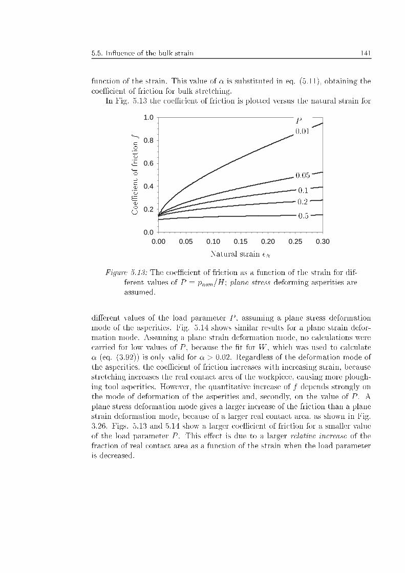
5.5. In uence of the bulk strain 141
function of the strain. This value of � is substituted in eq. (5.11), obtaining thecoeÆcient of friction for bulk stretching.
In Fig. 5.13 the coeÆcient of friction is plotted versus the natural strain for
0.00 0.05 0.10 0.15 0.20 0.25 0.300.0
0.2
0.4
0.6
0.8
1.0
Natural strain �N
Coe Æc ientoffrictio nf
0:01
0:05
0:1
0:2
0:5
P =
Figure 5.13: The coeÆcient of friction as a function of the strain for dif-ferent values of P = pnom=H; plane stress deforming asperities areassumed.
di�erent values of the load parameter P , assuming a plane stress deformationmode of the asperities. Fig. 5.14 shows similar results for a plane strain defor-mation mode. Assuming a plane strain deformation mode, no calculations werecarried for low values of P , because the �t for W , which was used to calculate� (eq. (3.92)) is only valid for � > 0:02. Regardless of the deformation mode ofthe asperities, the coeÆcient of friction increases with increasing strain, becausestretching increases the real contact area of the workpiece, causing more plough-ing tool asperities. However, the quantitative increase of f depends strongly onthe mode of deformation of the asperities and, secondly, on the value of P . Aplane stress deformation mode gives a larger increase of the friction than a planestrain deformation mode, because of a larger real contact area, as shown in Fig.3.26. Figs. 5.13 and 5.14 show a larger coeÆcient of friction for a smaller valueof the load parameter P . This e�ect is due to a larger relative increase of thefraction of real contact area as a function of the strain when the load parameteris decreased.
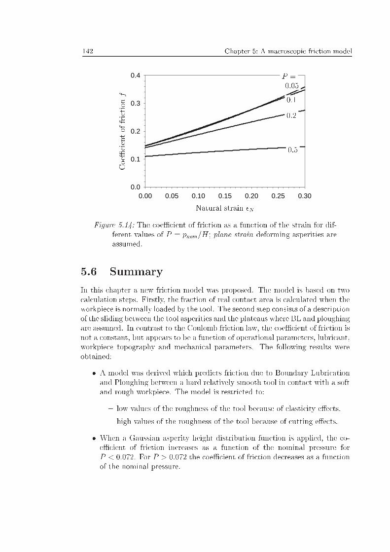
142 Chapter 5: A macroscopic friction model
0.00 0.05 0.10 0.15 0.20 0.25 0.300.0
0.1
0.2
0.3
0.4
Natural strain �N
CoeÆcientoffrictio nf
0:05
0:1
0:2
0:5
P =
Figure 5.14: The coeÆcient of friction as a function of the strain for dif-ferent values of P = pnom=H; plane strain deforming asperities areassumed.
5.6 Summary
In this chapter a new friction model was proposed. The model is based on twocalculation steps. Firstly, the fraction of real contact area is calculated when theworkpiece is normally loaded by the tool. The second step consists of a descriptionof the sliding between the tool asperities and the plateaus where BL and ploughingare assumed. In contrast to the Coulomb friction law, the coeÆcient of friction isnot a constant, but appears to be a function of operational parameters, lubricant,workpiece topography and mechanical parameters. The following results wereobtained:
� A model was derived which predicts friction due to Boundary Lubricationand Ploughing between a hard relatively smooth tool in contact with a softand rough workpiece. The model is restricted to:
{ low values of the roughness of the tool because of elasticity e�ects.
{ high values of the roughness of the tool because of cutting e�ects.
� When a Gaussian asperity height distribution function is applied, the co-eÆcient of friction increases as a function of the nominal pressure forP < 0:072. For P > 0:072 the coeÆcient of friction decreases as a functionof the nominal pressure.
5.6. Summary 143
� With a Gaussian asperity height distribution function, harder surfaces re-sult in a lower coeÆcient of friction for low values of P and a larger coeÆ-cient of friction for large values of P .
� A larger shear strength of the boundary layers gives a larger overall coeÆ-cient of friction.
� Application of non-Gaussian distribution functions in uences the relationbetween the friction and the load parameter P .
� Application of a bulk strain leads to a larger friction, due to enhanced attening (roughening is not taken into account). The increase is larger fora plane stress than for a plane strain deformation mode of the asperitiesand for lower values of P .
The model, which was derived in this chapter, will be veri�ed in the followingchapter.

144 Chapter 5: A macroscopic friction model
Chapter 6
Experimental validation of thefriction model
In chapter 5 the friction model with application to deep drawing processes wasdescribed. In this chapter friction experiments for the veri�cation of this modelwill be discussed.
The experimental devices, which were used for the friction experiments, arediscussed in section 6.1. The speci�cations of the workpiece materials, the toolmaterials and the lubricants are presented in section 6.2. The experimental pro-cedures are explained in section 6.3. The in uence of the roughness of the tool onthe friction is described both from an experimental and theoretical point of viewin section 6.4. In section 6.5 the e�ect of the pressure for line and at contactsis studied. Finally, in section 6.6 the results are discussed.
6.1 Experimental devices
A number of experimental devices was used to validate the friction model. In thefollowing, the RON-tester and the S-tribometer will be discussed. Appendix Dgives a photographic impression of both test devices.
6.1.1 The RON-tester
In Fig. 6.1 the so-called RON-tester is shown developed by ter Haar (1996).It consists of a tensile tester and a friction measuring device. The test devicewas specially developed for simulating SMF-processes. A strip of sheet metal isclamped in the tensile tester and can be either elastically or plastically deformed.
The friction-measuring device unit is able to move along the strip by means ofturning a spindle, which is driven by a servo-motor. Two hardened steel cylindersare mounted on the friction-measuring device unit. The rotating cylinder has a
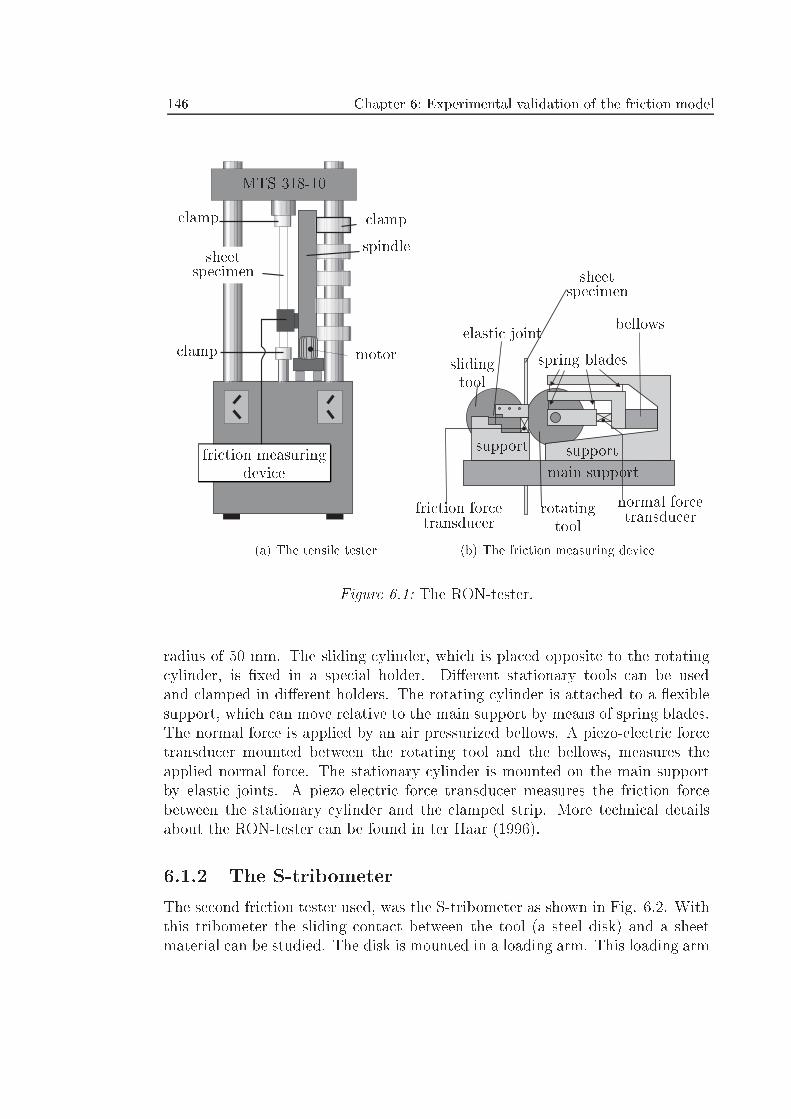
146 Chapter 6: Experimental validation of the friction model
clamp
MTS 318-10
clamp
sheetspecimen
spindle
clamp motor
friction measuringdevice
(a) The tensile tester
sheetspecimen
elastic joint
slidingtool
friction forcetransducer
rotatingtool
main support
support
normal forcetransducer
bellows
spring blades
support
(b) The friction measuring device
Figure 6.1: The RON-tester.
radius of 50 mm. The sliding cylinder, which is placed opposite to the rotatingcylinder, is �xed in a special holder. Di�erent stationary tools can be usedand clamped in di�erent holders. The rotating cylinder is attached to a exiblesupport, which can move relative to the main support by means of spring blades.The normal force is applied by an air pressurized bellows. A piezo-electric forcetransducer mounted between the rotating tool and the bellows, measures theapplied normal force. The stationary cylinder is mounted on the main supportby elastic joints. A piezo-electric force transducer measures the friction forcebetween the stationary cylinder and the clamped strip. More technical detailsabout the RON-tester can be found in ter Haar (1996).
6.1.2 The S-tribometer
The second friction tester used, was the S-tribometer as shown in Fig. 6.2. Withthis tribometer the sliding contact between the tool (a steel disk) and a sheetmaterial can be studied. The disk is mounted in a loading arm. This loading arm
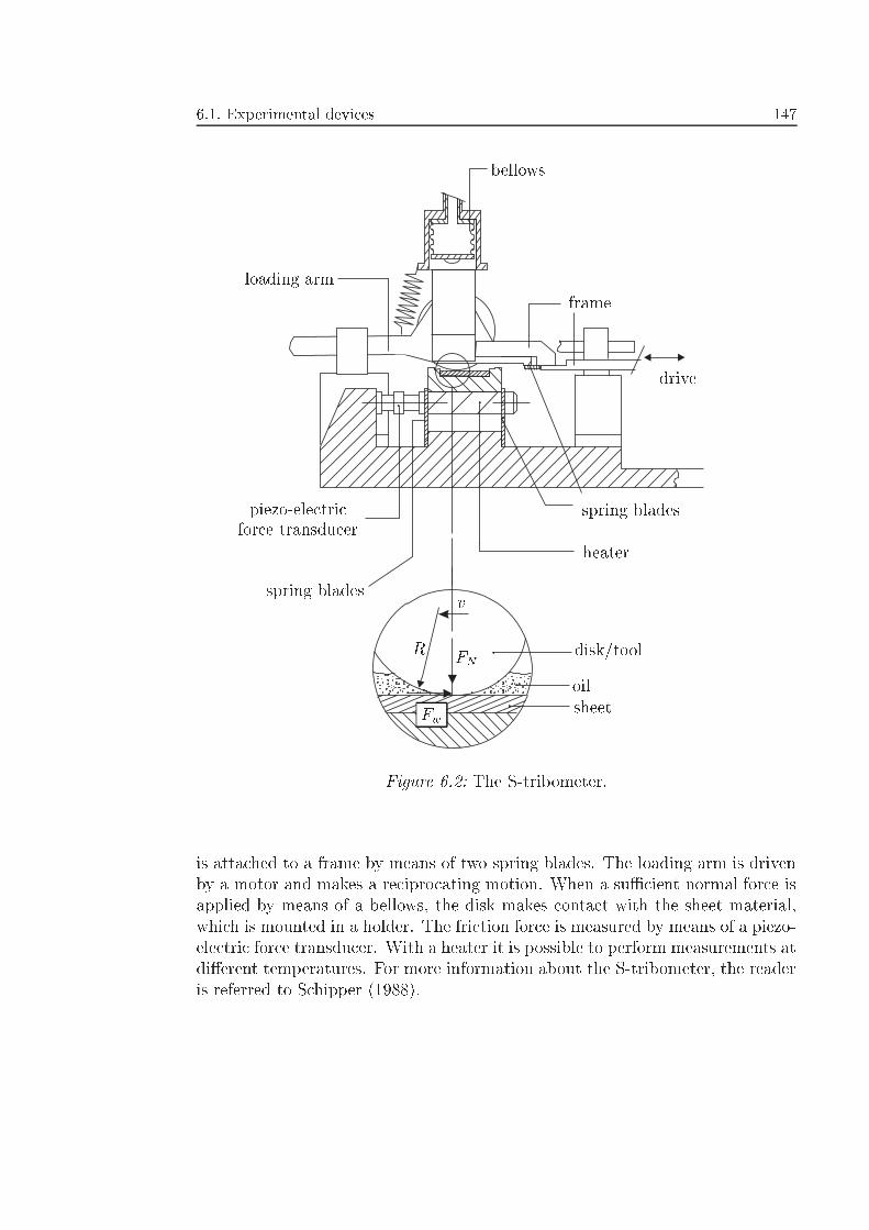
6.1. Experimental devices 147
loading arm
bellows
frame
drive
spring blades
heater
piezo-electricforce transducer
spring blades
disk/tool
oilsheet
v
FNR
Fw
Figure 6.2: The S-tribometer.
is attached to a frame by means of two spring blades. The loading arm is drivenby a motor and makes a reciprocating motion. When a suÆcient normal force isapplied by means of a bellows, the disk makes contact with the sheet material,which is mounted in a holder. The friction force is measured by means of a piezo-electric force transducer. With a heater it is possible to perform measurements atdi�erent temperatures. For more information about the S-tribometer, the readeris referred to Schipper (1988).
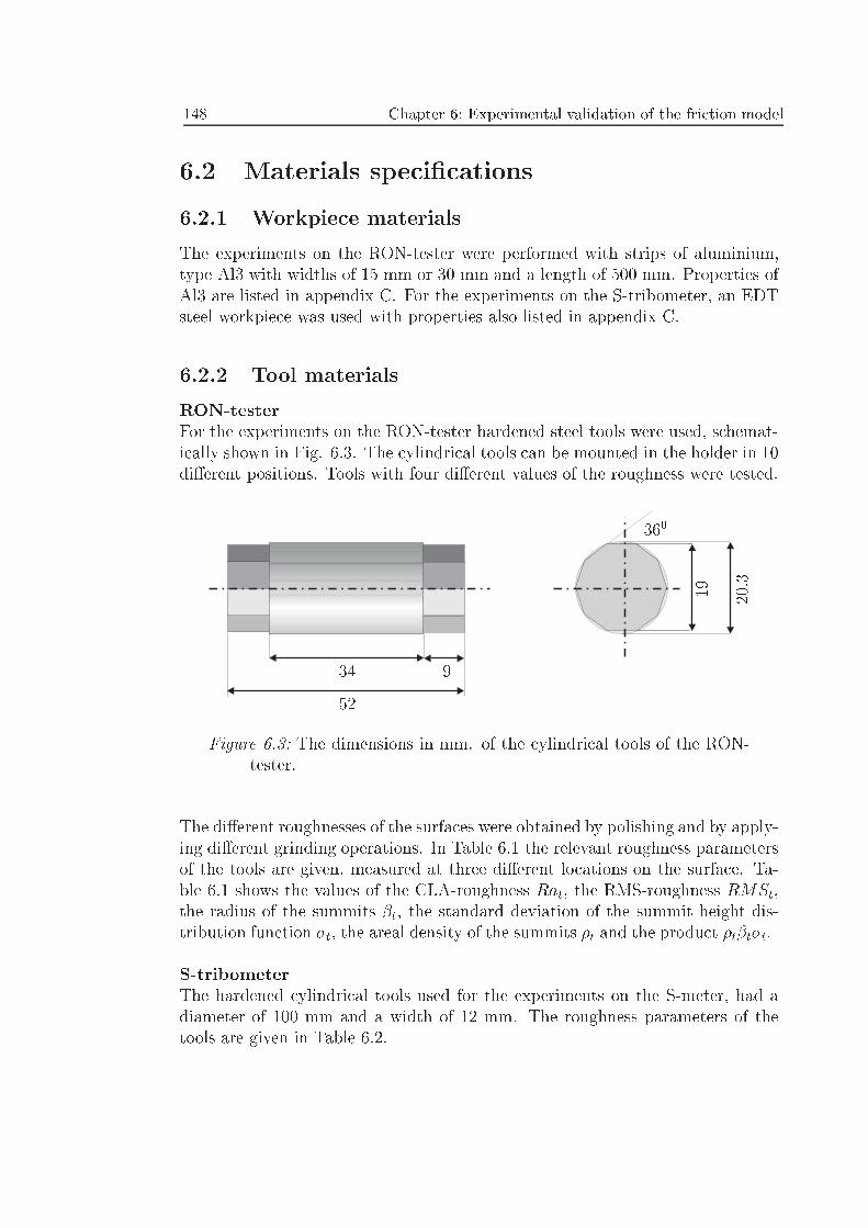
148 Chapter 6: Experimental validation of the friction model
6.2 Materials speci�cations
6.2.1 Workpiece materials
The experiments on the RON-tester were performed with strips of aluminium,type Al3 with widths of 15 mm or 30 mm and a length of 500 mm. Properties ofAl3 are listed in appendix C. For the experiments on the S-tribometer, an EDTsteel workpiece was used with properties also listed in appendix C.
6.2.2 Tool materials
RON-testerFor the experiments on the RON-tester hardened steel tools were used, schemat-ically shown in Fig. 6.3. The cylindrical tools can be mounted in the holder in 10di�erent positions. Tools with four di�erent values of the roughness were tested.
34
52
9
360
19 20.3
Figure 6.3: The dimensions in mm. of the cylindrical tools of the RON-tester.
The di�erent roughnesses of the surfaces were obtained by polishing and by apply-ing di�erent grinding operations. In Table 6.1 the relevant roughness parametersof the tools are given, measured at three di�erent locations on the surface. Ta-ble 6.1 shows the values of the CLA-roughness Rat, the RMS-roughness RMSt,the radius of the summits �t, the standard deviation of the summit height dis-tribution function �t, the areal density of the summits �t and the product �t�t�t.
S-tribometerThe hardened cylindrical tools used for the experiments on the S-meter, had adiameter of 100 mm and a width of 12 mm. The roughness parameters of thetools are given in Table 6.2.
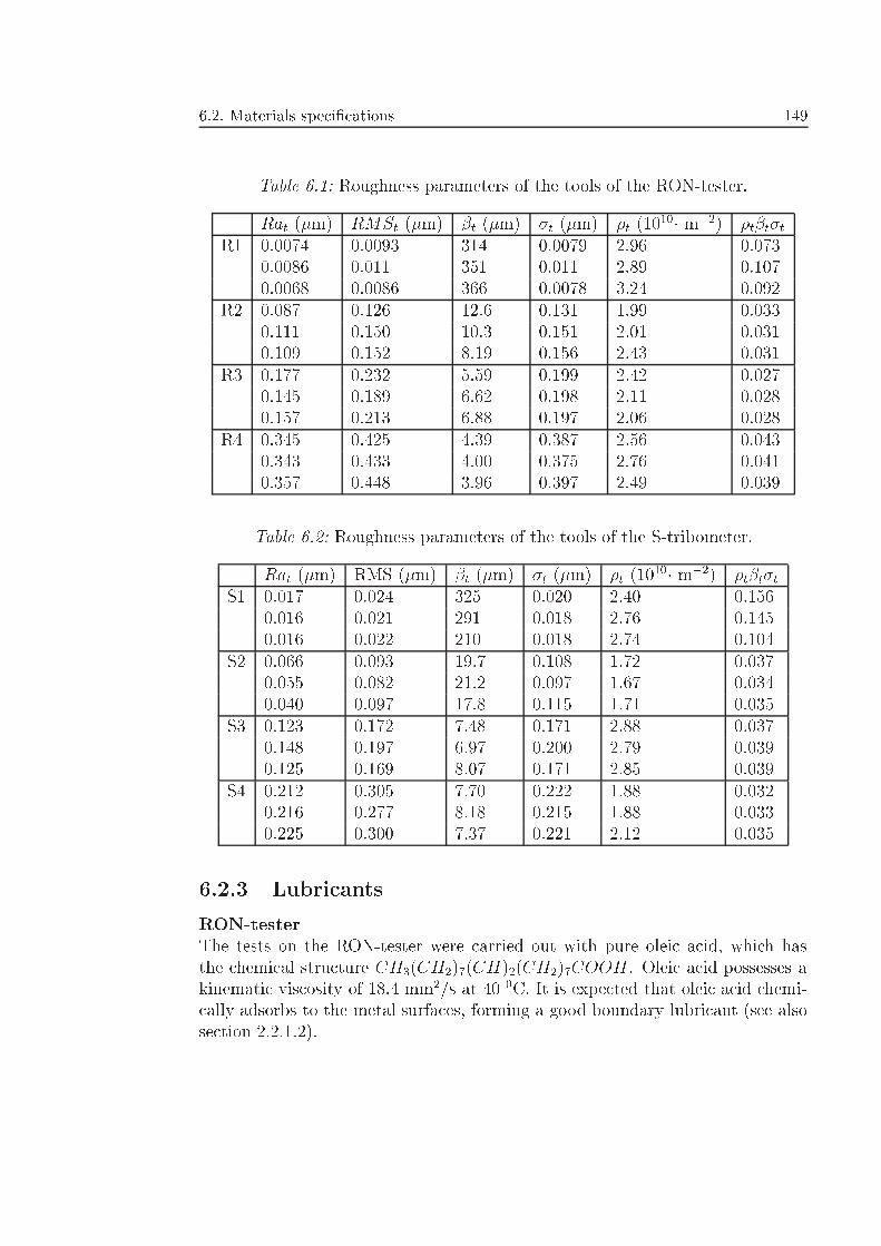
6.2. Materials speci�cations 149
Table 6.1: Roughness parameters of the tools of the RON-tester.
Rat (�m) RMSt (�m) �t (�m) �t (�m) �t (1010� m�2) �t�t�t
R1 0.0074 0.0093 314 0.0079 2.96 0.0730.0086 0.011 351 0.011 2.89 0.1070.0068 0.0086 366 0.0078 3.24 0.092
R2 0.087 0.126 12.6 0.131 1.99 0.0330.111 0.150 10.3 0.151 2.01 0.0310.109 0.152 8.19 0.156 2.43 0.031
R3 0.177 0.232 5.59 0.199 2.42 0.0270.145 0.189 6.62 0.198 2.11 0.0280.157 0.213 6.88 0.197 2.06 0.028
R4 0.345 0.425 4.39 0.387 2.56 0.0430.343 0.433 4.00 0.375 2.76 0.0410.357 0.448 3.96 0.397 2.49 0.039
Table 6.2: Roughness parameters of the tools of the S-tribometer.
Rat (�m) RMS (�m) �t (�m) �t (�m) �t (1010� m�2) �t�t�t
S1 0.017 0.024 325 0.020 2.40 0.1560.016 0.021 291 0.018 2.76 0.1450.016 0.022 210 0.018 2.74 0.104
S2 0.066 0.093 19.7 0.108 1.72 0.0370.055 0.082 21.2 0.097 1.67 0.0340.040 0.097 17.8 0.115 1.71 0.035
S3 0.123 0.172 7.48 0.171 2.88 0.0370.148 0.197 6.97 0.200 2.79 0.0390.125 0.169 8.07 0.171 2.85 0.039
S4 0.212 0.305 7.70 0.222 1.88 0.0320.216 0.277 8.18 0.215 1.88 0.0330.225 0.300 7.37 0.221 2.12 0.035
6.2.3 Lubricants
RON-testerThe tests on the RON-tester were carried out with pure oleic acid, which hasthe chemical structure CH3(CH2)7(CH)2(CH2)7COOH. Oleic acid possesses akinematic viscosity of 18.4 mm2/s at 40 0C. It is expected that oleic acid chemi-cally adsorbs to the metal surfaces, forming a good boundary lubricant (see alsosection 2.2.1.2).
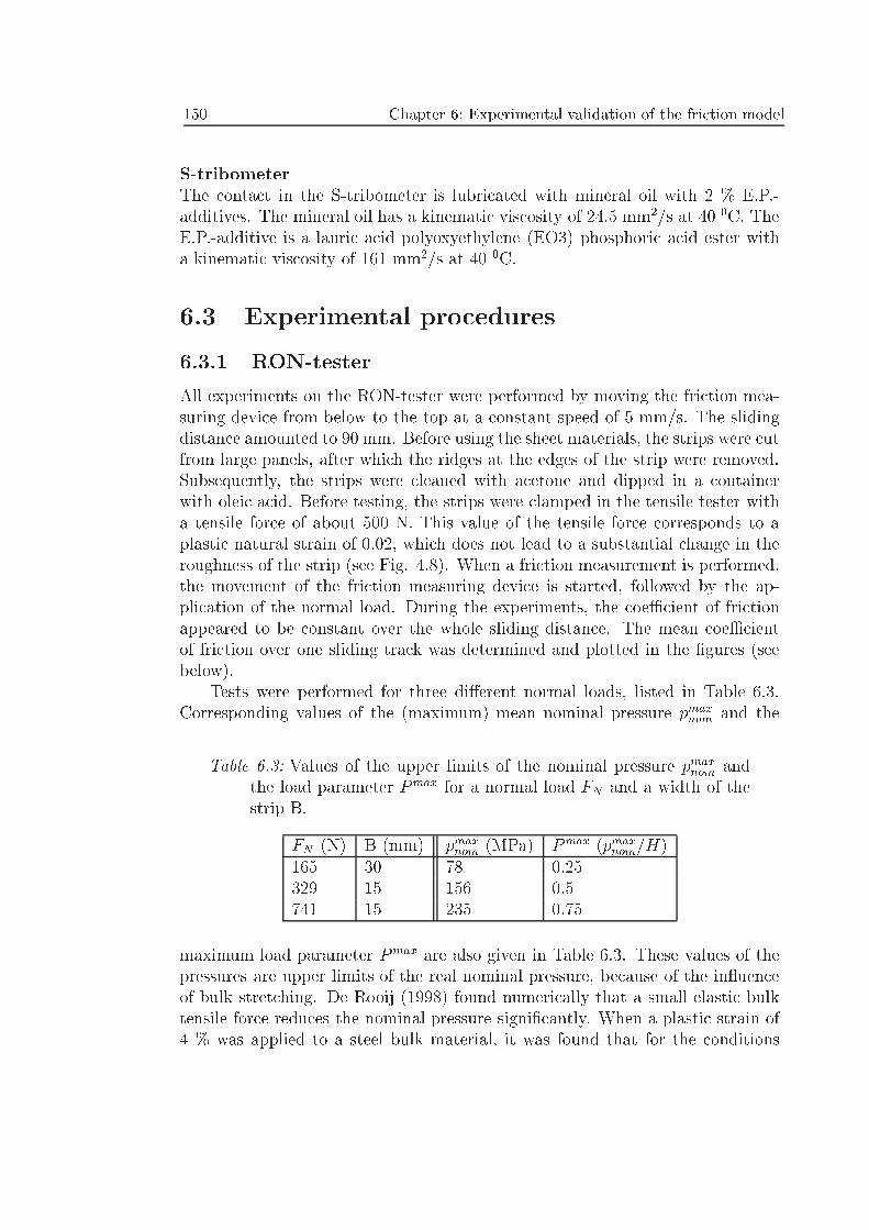
150 Chapter 6: Experimental validation of the friction model
S-tribometerThe contact in the S-tribometer is lubricated with mineral oil with 2 % E.P.-additives. The mineral oil has a kinematic viscosity of 24.5 mm2/s at 40 0C. TheE.P.-additive is a lauric acid polyoxyethylene (EO3) phosphoric acid ester witha kinematic viscosity of 161 mm2/s at 40 0C.
6.3 Experimental procedures
6.3.1 RON-tester
All experiments on the RON-tester were performed by moving the friction mea-suring device from below to the top at a constant speed of 5 mm/s. The slidingdistance amounted to 90 mm. Before using the sheet materials, the strips were cutfrom large panels, after which the ridges at the edges of the strip were removed.Subsequently, the strips were cleaned with acetone and dipped in a containerwith oleic acid. Before testing, the strips were clamped in the tensile tester witha tensile force of about 500 N. This value of the tensile force corresponds to aplastic natural strain of 0.02, which does not lead to a substantial change in theroughness of the strip (see Fig. 4.8). When a friction measurement is performed,the movement of the friction measuring device is started, followed by the ap-plication of the normal load. During the experiments, the coeÆcient of frictionappeared to be constant over the whole sliding distance. The mean coeÆcientof friction over one sliding track was determined and plotted in the �gures (seebelow).
Tests were performed for three di�erent normal loads, listed in Table 6.3.Corresponding values of the (maximum) mean nominal pressure pmaxnom and the
Table 6.3: Values of the upper limits of the nominal pressure pmaxnom andthe load parameter Pmax for a normal load FN and a width of thestrip B.
FN (N) B (mm) pmaxnom (MPa) Pmax (pmaxnom=H)165 30 78 0.25329 15 156 0.5741 15 235 0.75
maximum load parameter Pmax are also given in Table 6.3. These values of thepressures are upper limits of the real nominal pressure, because of the in uenceof bulk stretching. De Rooij (1998) found numerically that a small elastic bulktensile force reduces the nominal pressure signi�cantly. When a plastic strain of4 % was applied to a steel bulk material, it was found that for the conditions
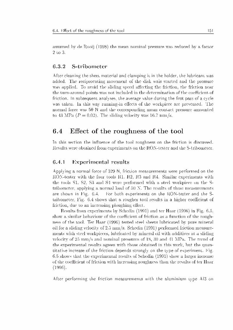
6.4. E�ect of the roughness of the tool 151
assumed by de Rooij (1998) the mean nominal pressure was reduced by a factor2 to 3.
6.3.2 S-tribometer
After cleaning the sheet material and clamping it in the holder, the lubricant wasadded. The reciprocating movement of the disk wais started and the pressurewas applied. To avoid the sliding speed a�ecting the friction, the friction nearthe turn-around points was not included in the determination of the coeÆcient offriction. In subsequent analyses, the average value during the �rst pass of a cyclewas taken. In this way running-in e�ects of the workpiece are prevented. Thenormal force was 50 N and the corresponding mean contact pressure amountedto 43 MPa (P = 0:02). The sliding velocity was 16.7 mm/s.
6.4 E�ect of the roughness of the tool
In this section the in uence of the tool roughness on the friction is discussed.Results were obtained from experiments on the RON-tester and the S-tribometer.
6.4.1 Experimental results
Applying a normal force of 329 N, friction measurements were performed on theRON-tester with the four tools R1, R2, R3 and R4. Similar experiments withthe tools S1, S2, S3 and S4 were performed with a steel workpiece on the S-tribometer, applying a normal load of 50 N. The results of these measurementsare shown in Fig. 6.4. For both experiments on the RON-tester and the S-tribometer, Fig. 6.4 shows that a rougher tool results in a higher coeÆcient offriction, due to an increasing ploughing e�ect.
Results from experiments by Schedin (1991) and ter Haar (1996) in Fig. 6.5,show a similar behaviour of the coeÆcient of friction as a function of the rough-ness of the tool. Ter Haar (1996) tested steel sheets lubricated by pure mineraloil for a sliding velocity of 2.5 mm/s. Schedin (1991) performed friction measure-ments with steel workpieces, lubricated by mineral oil with additives at a slidingvelocity of 25 mm/s and nominal pressures of 18, 30 and 41 MPa. The trend ofthe experimental results agrees with those obtained in this work, but the quan-titative increase of the friction depends strongly on the type of experiment. Fig.6.5 shows that the experimental results of Schedin (1991) show a larger increaseof the coeÆcient of friction with increasing roughness than the results of ter Haar(1996).
After performing the friction measurements with the aluminium type Al3 on
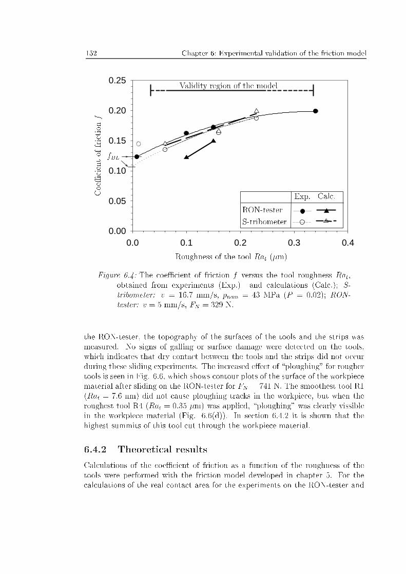
152 Chapter 6: Experimental validation of the friction model
0.0 0.1 0.2 0.3 0.40.00
0.05
0.10
0.15
0.20
0.25
Roughness of the tool Rat (�m)
CoeÆcientoffrictio nf
Exp. Calc.
RON-tester
S-tribometer
Validity region of the model
fBL
Figure 6.4: The coeÆcient of friction f versus the tool roughness Rat,obtained from experiments (Exp.) and calculations (Calc.); S-tribometer: v = 16:7 mm/s, pnom = 43 MPa (P = 0:02); RON-tester: v = 5 mm/s, FN = 329 N.
the RON-tester, the topography of the surfaces of the tools and the strips wasmeasured. No signs of galling or surface damage were detected on the tools,which indicates that dry contact between the tools and the strips did not occurduring these sliding experiments. The increased e�ect of \ploughing" for roughertools is seen in Fig. 6.6, which shows contour plots of the surface of the workpiecematerial after sliding on the RON-tester for FN = 741 N. The smoothest tool R1(Rat = 7:6 nm) did not cause ploughing tracks in the workpiece, but when theroughest tool R4 (Rat = 0:35 �m) was applied, \ploughing" was clearly vissiblein the workpiece material (Fig. 6.6(d)). In section 6.4.2 it is shown that thehighest summits of this tool cut through the workpiece material.
6.4.2 Theoretical results
Calculations of the coeÆcient of friction as a function of the roughness of thetools were performed with the friction model developed in chapter 5. For thecalculations of the real contact area for the experiments on the RON-tester and
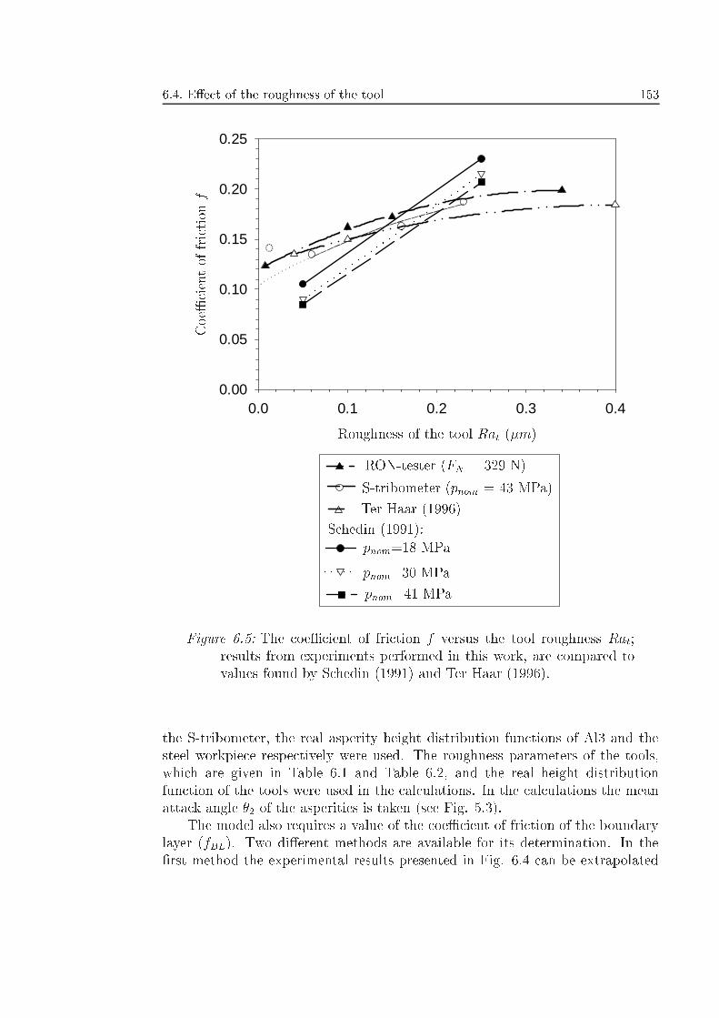
6.4. E�ect of the roughness of the tool 153
0.0 0.1 0.2 0.3 0.40.00
0.05
0.10
0.15
0.20
0.25
Roughness of the tool Rat (�m)
CoeÆcientoffrictio nf
S-tribometer (pnom = 43 MPa)
Ter Haar (1996)
Schedin (1991):
pnom=18 MPa
pnom=30 MPa
pnom=41 MPa
RON-tester (FN = 329 N)
Figure 6.5: The coeÆcient of friction f versus the tool roughness Rat;results from experiments performed in this work, are compared tovalues found by Schedin (1991) and Ter Haar (1996).
the S-tribometer, the real asperity height distribution functions of Al3 and thesteel workpiece respectively were used. The roughness parameters of the tools,which are given in Table 6.1 and Table 6.2, and the real height distributionfunction of the tools were used in the calculations. In the calculations the meanattack angle �2 of the asperities is taken (see Fig. 5.3).
The model also requires a value of the coeÆcient of friction of the boundarylayer (fBL). Two di�erent methods are available for its determination. In the�rst method the experimental results presented in Fig. 6.4 can be extrapolated
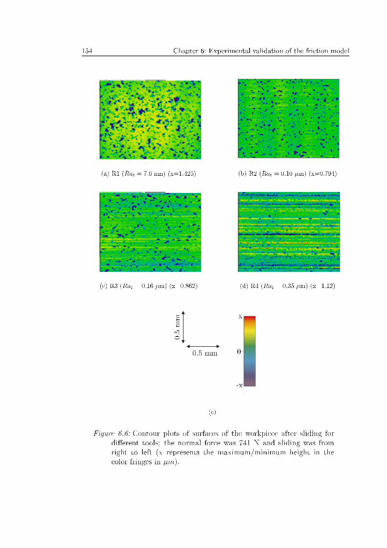
154 Chapter 6: Experimental validation of the friction model
(a) R1 (Rat = 7:6 nm) (x=1.425) (b) R2 (Rat = 0:10 �m) (x=0.794)
(c) R3 (Rat = 0:16 �m) (x=0.862) (d) R4 (Rat = 0:35 �m) (x=1.12)
x
0
-x
0.5 mm
0.5mm
(e)
Figure 6.6: Contour plots of surfaces of the workpiece after sliding fordi�erent tools; the normal force was 741 N and sliding was fromright to left (x represents the maximum/minimum height in thecolor fringes in �m).
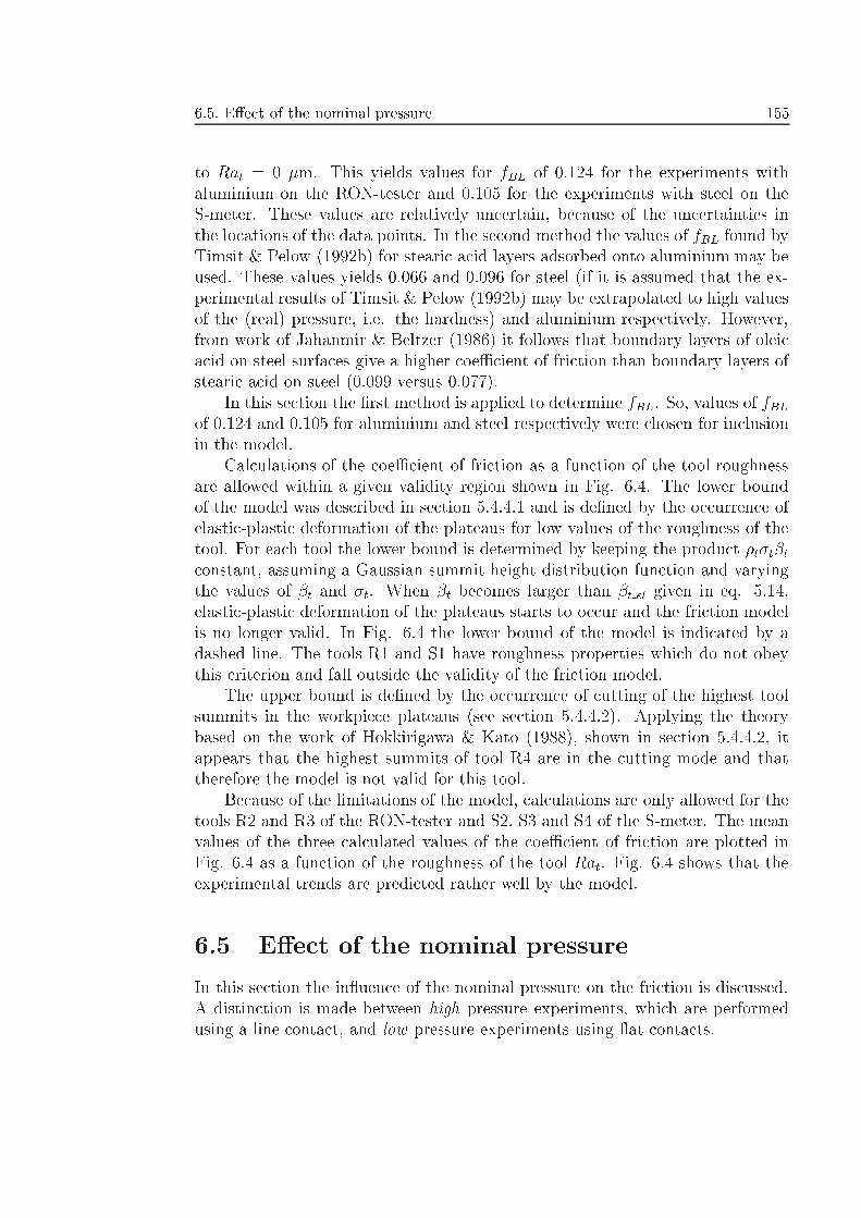
6.5. E�ect of the nominal pressure 155
to Rat = 0 �m. This yields values for fBL of 0.124 for the experiments withaluminium on the RON-tester and 0.105 for the experiments with steel on theS-meter. These values are relatively uncertain, because of the uncertainties inthe locations of the data points. In the second method the values of fBL found byTimsit & Pelow (1992b) for stearic acid layers adsorbed onto aluminium may beused. These values yields 0.066 and 0.096 for steel (if it is assumed that the ex-perimental results of Timsit & Pelow (1992b) may be extrapolated to high valuesof the (real) pressure, i.e. the hardness) and aluminium respectively. However,from work of Jahanmir & Beltzer (1986) it follows that boundary layers of oleicacid on steel surfaces give a higher coeÆcient of friction than boundary layers ofstearic acid on steel (0.099 versus 0.077).
In this section the �rst method is applied to determine fBL. So, values of fBLof 0.124 and 0.105 for aluminium and steel respectively were chosen for inclusionin the model.
Calculations of the coeÆcient of friction as a function of the tool roughnessare allowed within a given validity region shown in Fig. 6.4. The lower boundof the model was described in section 5.4.4.1 and is de�ned by the occurrence ofelastic-plastic deformation of the plateaus for low values of the roughness of thetool. For each tool the lower bound is determined by keeping the product �t�t�tconstant, assuming a Gaussian summit height distribution function and varyingthe values of �t and �t. When �t becomes larger than �t el given in eq. 5.14,elastic-plastic deformation of the plateaus starts to occur and the friction modelis no longer valid. In Fig. 6.4 the lower bound of the model is indicated by adashed line. The tools R1 and S1 have roughness properties which do not obeythis criterion and fall outside the validity of the friction model.
The upper bound is de�ned by the occurrence of cutting of the highest toolsummits in the workpiece plateaus (see section 5.4.4.2). Applying the theorybased on the work of Hokkirigawa & Kato (1988), shown in section 5.4.4.2, itappears that the highest summits of tool R4 are in the cutting mode and thattherefore the model is not valid for this tool.
Because of the limitations of the model, calculations are only allowed for thetools R2 and R3 of the RON-tester and S2, S3 and S4 of the S-meter. The meanvalues of the three calculated values of the coeÆcient of friction are plotted inFig. 6.4 as a function of the roughness of the tool Rat. Fig. 6.4 shows that theexperimental trends are predicted rather well by the model.
6.5 E�ect of the nominal pressure
In this section the in uence of the nominal pressure on the friction is discussed.A distinction is made between high pressure experiments, which are performedusing a line contact, and low pressure experiments using at contacts.
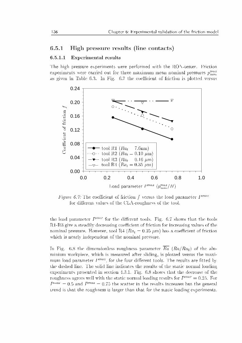
156 Chapter 6: Experimental validation of the friction model
6.5.1 High pressure results (line contacts)
6.5.1.1 Experimental results
The high pressure experiments were performed with the RON-tester. Frictionexperiments were carried out for three maximum mean nominal pressures pmaxnom
as given in Table 6.3. In Fig. 6.7 the coeÆcient of friction is plotted versus
0.0 0.2 0.4 0.6 0.8 1.00.00
0.04
0.08
0.12
0.16
0.20
0.24
Load parameter Pmax (pmaxnom=H)
CoeÆcientoffrictionf
tool R1 (Rat = 7:6nm)tool R2 (Rat = 0:10 �m)tool R3 (Rat = 0:16 �m)tool R4 (Rat = 0:35 �m)
Figure 6.7: The coeÆcient of friction f versus the load parameter Pmax
for di�erent values of the CLA-roughness of the tool.
the load parameter Pmax for the di�erent tools. Fig. 6.7 shows that the toolsR1-R3 give a steadily decreasing coeÆcient of friction for increasing values of thenominal pressure. However, tool R4 (Rat = 0.35 �m) has a coeÆcient of frictionwhich is nearly independent of the nominal pressure.
In Fig. 6.8 the dimensionless roughness parameter Ra (Ra=Ra0) of the alu-minium workpiece, which is measured after sliding, is plotted versus the maxi-mum load parameter Pmax, for the four di�erent tools. The results are �tted bythe dashed line. The solid line indicates the results of the static normal loadingexperiments presented in section 4.3.1. Fig. 6.8 shows that the decrease of theroughness agrees well with the static normal loading results for Pmax = 0:25. ForPmax = 0:5 and Pmax = 0:75 the scatter in the results increases but the generaltrend is that the roughness is larger than that for the static loading experiments.
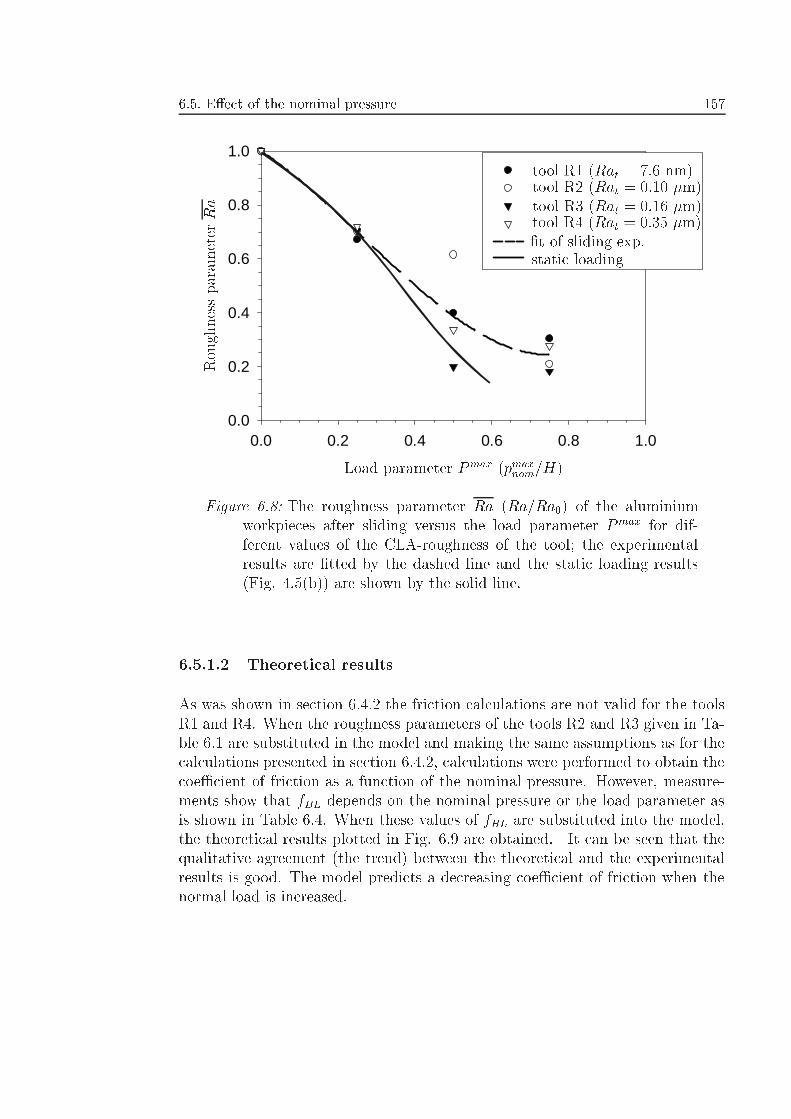
6.5. E�ect of the nominal pressure 157
0.0 0.2 0.4 0.6 0.8 1.00.0
0.2
0.4
0.6
0.8
1.0
Load parameter Pmax (pmaxnom=H)
RoughnessparameterRa
tool R1 (Rat = 7:6 nm)tool R2 (Rat = 0:10 �m)tool R3 (Rat = 0:16 �m)tool R4 (Rat = 0:35 �m)
static loading�t of sliding exp.
Figure 6.8: The roughness parameter Ra (Ra=Ra0) of the aluminiumworkpieces after sliding versus the load parameter Pmax for dif-ferent values of the CLA-roughness of the tool; the experimentalresults are �tted by the dashed line and the static loading results(Fig. 4.5(b)) are shown by the solid line.
6.5.1.2 Theoretical results
As was shown in section 6.4.2 the friction calculations are not valid for the toolsR1 and R4. When the roughness parameters of the tools R2 and R3 given in Ta-ble 6.1 are substituted in the model and making the same assumptions as for thecalculations presented in section 6.4.2, calculations were performed to obtain thecoeÆcient of friction as a function of the nominal pressure. However, measure-ments show that fBL depends on the nominal pressure or the load parameter asis shown in Table 6.4. When these values of fBL are substituted into the model,the theoretical results plotted in Fig. 6.9 are obtained. It can be seen that thequalitative agreement (the trend) between the theoretical and the experimentalresults is good. The model predicts a decreasing coeÆcient of friction when thenormal load is increased.
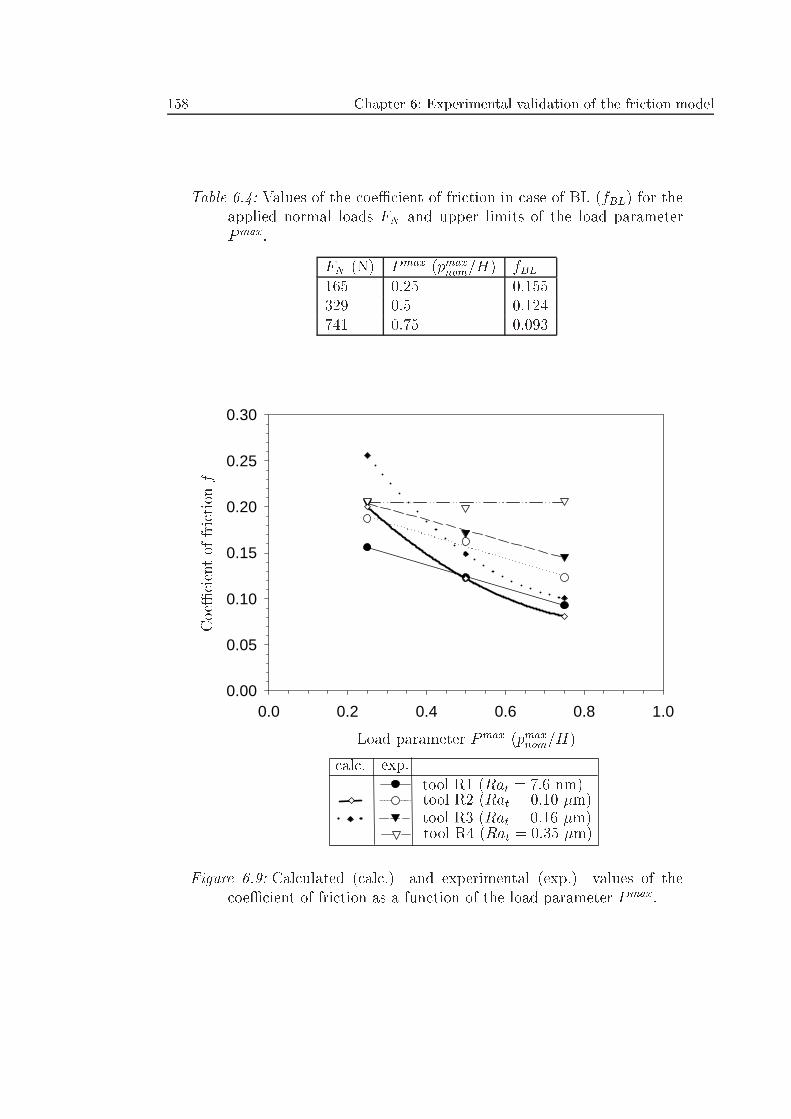
158 Chapter 6: Experimental validation of the friction model
Table 6.4: Values of the coeÆcient of friction in case of BL (fBL) for theapplied normal loads FN and upper limits of the load parameterPmax.
FN (N) Pmax (pmaxnom=H) fBL165 0.25 0.155329 0.5 0.124741 0.75 0.093
0.0 0.2 0.4 0.6 0.8 1.00.00
0.05
0.10
0.15
0.20
0.25
0.30
Load parameter Pmax (pmaxnom=H)
CoeÆcientoffrictionf
tool R1 (Rat = 7:6 nm)tool R2 (Rat = 0:10 �m)tool R3 (Rat = 0:16 �m)tool R4 (Rat = 0:35 �m)
calc. exp.
Figure 6.9: Calculated (calc.) and experimental (exp.) values of thecoeÆcient of friction as a function of the load parameter Pmax.
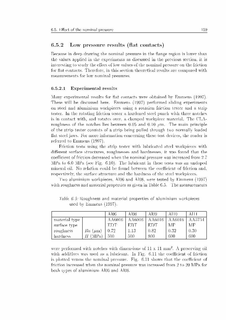
6.5. E�ect of the nominal pressure 159
6.5.2 Low pressure results ( at contacts)
Because in deep drawing the nominal pressure in the ange region is lower thanthe values applied in the experiments as discussed in the previous section, it isinteresting to study the e�ect of low values of the nominal pressure on the frictionfor at contacts. Therefore, in this section theoretical results are compared withmeasurements for low nominal pressures.
6.5.2.1 Experimental results
Many experimental results for at contacts were obtained by Emmens (1997).These will be discussed here. Emmens (1997) performed sliding experimentson steel and aluminium workpieces using a rotation friction tester and a striptester. In the rotating friction tester a hardened steel punch with three notchesis in contact with, and rotates over, a clamped workpiece material. The CLA-roughness of the notches lies between 0.05 and 0.10 �m. The main principleof the strip tester consists of a strip being pulled through two normally loaded at steel jaws. For more information concerning these test devices, the reader isreferred to Emmens (1997).
Friction tests using the strip tester with lubricated steel workpieces withdi�erent surface structures, roughnesses and hardnesses, it was found that thecoeÆcient of friction decreased when the nominal pressure was increased from 2.7MPa to 6.0 MPa (see Fig. 6.10). The lubricant in these tests was an undopedmineral oil. No relation could be found between the coeÆcient of friction and,respectively, the surface structure and the hardness of the steel workpieces.
Two aluminium workpieces, Al06 and Al08, were tested by Emmens (1997)with roughness and material properties as given in Table 6.5. The measurements
Table 6.5: Roughness and material properties of aluminium workpiecesused by Emmens (1997).
Al06 Al08 Al09 Al10 Al11material type AA6016 AA6016 AA6016 AA6016 AA5754surface type EDT EBT EDT MF MFroughness Ra (�m) 0.72 1.13 0.82 0.32 0.30hardness H (MPa) 500 500 800 600 600
were performed with notches with dimensions of 11 x 11 mm2. A preserving oilwith additives was used as a lubricant. In Fig. 6.11 the coeÆcient of frictionis plotted versus the nominal pressure. Fig. 6.11 shows that the coeÆcient offriction increased when the nominal pressure was increased from 2 to 20 MPa forboth types of aluminium Al06 and Al08.
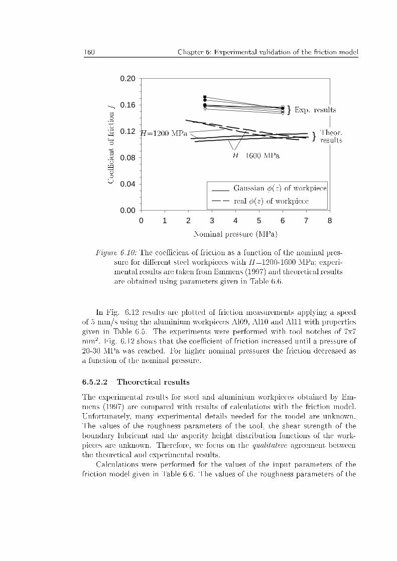
160 Chapter 6: Experimental validation of the friction model
0 1 2 3 4 5 6 7 80.00
0.04
0.08
0.12
0.16
0.20
}
}
Nominal pressure (MPa)
CoeÆcientoffrictio nf Exp. results
Theor.results
H=1600 MPa
H=1200 MPa
Gaussian �(z) of workpiece
real �(z) of workpiece
Figure 6.10: The coeÆcient of friction as a function of the nominal pres-sure for di�erent steel workpieces with H=1200-1600 MPa; experi-mental results are taken from Emmens (1997) and theoretical resultsare obtained using parameters given in Table 6.6.
In Fig. 6.12 results are plotted of friction measurements applying a speedof 5 mm/s using the aluminium workpieces Al09, Al10 and Al11 with propertiesgiven in Table 6.5. The experiments were performed with tool notches of 7x7mm2. Fig. 6.12 shows that the coeÆcient of friction increased until a pressure of20-30 MPa was reached. For higher nominal pressures the friction decreased asa function of the nominal pressure.
6.5.2.2 Theoretical results
The experimental results for steel and aluminium workpieces obtained by Em-mens (1997) are compared with results of calculations with the friction model.Unfortunately, many experimental details needed for the model are unknown.The values of the roughness parameters of the tool, the shear strength of theboundary lubricant and the asperity height distribution functions of the work-pieces are unknown. Therefore, we focus on the qualitative agreement betweenthe theoretical and experimental results.
Calculations were performed for the values of the input parameters of thefriction model given in Table 6.6. The values of the roughness parameters of the
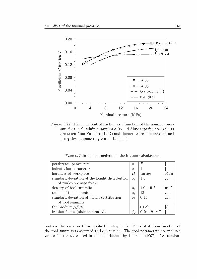
6.5. E�ect of the nominal pressure 161
0 4 8 12 16 20 240.00
0.04
0.08
0.12
0.16
0.20}
}
Nominal pressure (MPa)
CoeÆcientoffrictio nf
Al06
Al08
Exp. results
Theor.results
Gaussian �(z)
real �(z)
Figure 6.11: The coeÆcient of friction as a function of the nominal pres-sure for the aluminium samples Al06 and Al08; experimental resultsare taken from Emmens (1997) and theoretical results are obtainedusing the parameters given in Table 6.6.
Table 6.6: Input parameters for the friction calculations.
persistence parameter � P [-]indentation parameter n 1 [-]hardness of workpiece H varries MPastandard deviation of the height distribution �w 1.5 �m
of workpiece asperitiesdensity of tool summits �t 1:9 � 1010 m�2
radius of tool summits �t 13 �mstandard deviation of height distribution �t 0.15 �m
of tool summitsthe product �t�t�t 0.037 [-]friction factor (oleic acid on Al) fC 0:76 �H�0:19 [-]
tool are the same as those applied in chapter 5. The distribution function ofthe tool summits is assumed to be Gaussian. The tool parameters are realisticvalues for the tools used in the experiments by Emmens (1997). Calculations
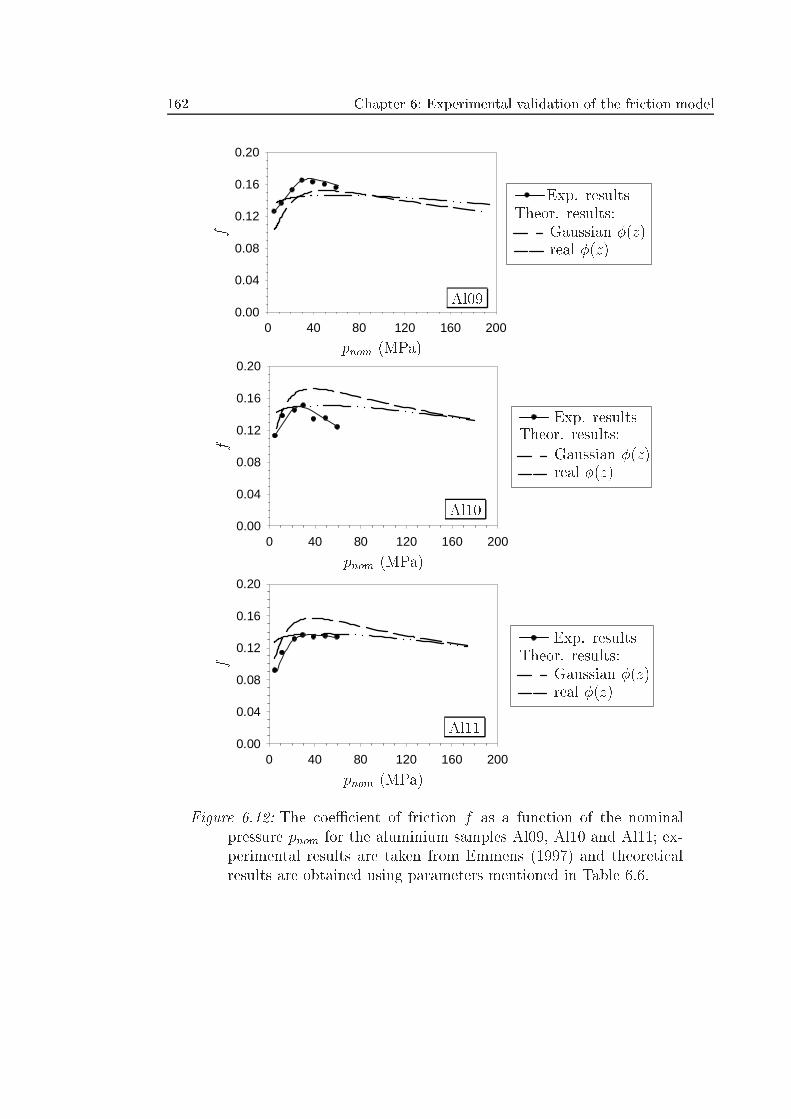
162 Chapter 6: Experimental validation of the friction model
0 40 80 120 160 2000.00
0.04
0.08
0.12
0.16
0.20
0 40 80 120 160 2000.00
0.04
0.08
0.12
0.16
0.20
0 40 80 120 160 2000.00
0.04
0.08
0.12
0.16
0.20
pnom (MPa)
pnom (MPa)
pnom (MPa)
f
f
f
Exp. results
Exp. results
Exp. results
Theor. results:
Theor. results:
Theor. results:
Gaussian �(z)
Gaussian �(z)
Gaussian �(z)
real �(z)
real �(z)
real �(z)
Al09
Al10
Al11
Figure 6.12: The coeÆcient of friction f as a function of the nominalpressure pnom for the aluminium samples Al09, Al10 and Al11; ex-perimental results are taken from Emmens (1997) and theoreticalresults are obtained using parameters mentioned in Table 6.6.
6.6. Discussion 163
were performed with a Gaussian and a real height distribution function �(z) ofthe workpiece asperities. As an example, the real distribution function of Al1 wasused (see Fig. 4.2), which is a typical height distribution for an EDT surface.Because the coeÆcient of friction under conditions of BL (fBL) is unknown, thefriction measurements for oleic acid boundary layers on aluminium by Timsit &Pelow (1992b) were used in the calculations. An expression for the friction factorfC as a function of the hardness of the workpiece H is given by eq. (5.13).
In Fig. 6.10 results are shown of calculations for steel surfaces with hardnessesbetween 1200 and 1600 MPa, which are the lowest and the largest values for thesteel workpieces tested by Emmens (1997). Substituting a Gaussian height dis-tribution function gives a coeÆcient of friction which increases when the nominalpressure is increased. However, when a real distribution function is substituted,the experimental trend is predicted well by the model. Although the coeÆcient offriction is underestimated, the experimental and theoretical results agree roughly,which is a satisfying result considering the many estimated input parameters ofthe model.
In Fig. 6.11 and Fig. 6.12 results are shown of calculations for the aluminiumworkpieces. Fig. 6.11 shows that the qualitative dependence of the coeÆcientof friction as a function of the nominal pressure is also predicted by the model.Bearing in mind the many estimated input parameters of the model, the theo-retical results are quite good. The shape of the theoretical curve, when a realdistribution function is used, agrees very well with the experimental one. Themeasured trend of the coeÆcient of friction as a function of the nominal pressure,shown in Fig. 6.12, is good for the real distribution function.
6.6 Discussion
6.6.1 E�ect of the roughness of the tool
The experimental results presented in Fig. 6.4 and Fig. 6.5 show that the greaterthe roughness of the tool, the greater the coeÆcient of friction, due to the in-creased contribution of ploughing to the overall friction.
The theoretical values of the coeÆcient of friction agree rather well with theexperimental values. The results for steel (S-meter experiments) are predicted es-pecially well by the model. The results for aluminium (RON-tester experiments)are slightly underestimated.
6.6.2 E�ect of the nominal pressure
6.6.2.1 High pressure results (line contacts)
The experiments on the RON-tester for di�erent tools and nominal pressures showthat for the smooth tools the coeÆcient of friction decreases when the nominal
164 Chapter 6: Experimental validation of the friction model
pressure is increased (see Fig. 6.7). This e�ect is also predicted by the model(see Fig. 6.9); it is due to the non-proportionality between the fraction of realcontact and the nominal pressure and the dependence of fBL as a function of thenominal pressure (see Table 6.4).
6.6.2.2 Low pressure results ( at contacts)
Substituting a real asperity distribution function for an EDT surface into thefriction model, the qualitative agreement between the experimental results ob-tained by Emmens (1997) for at contacts, and the theoretical results is rathergood. The results for sliding lubricated steel (Fig. 6.10) show an underestimatedcoeÆcient of friction. Possible causes may be the underestimated value of theshear strength of the boundary layer and the estimations of the distribution func-tion of the workpiece and the roughness parameters of the tool. The results foraluminium (Fig. 6.11 and Fig. 6.12) show that the trend of experimental and the-oretical results is similar. These results show that for low nominal pressures thecoeÆcient of friction increases when the nominal pressure is increased. For highnominal pressures the coeÆcient of friction decreases when the nominal pressureis increased.
Chapter 7
Conclusions andrecommendations
In this chapter conclusions of the present work and recommendations for furtherresearch are given.
7.1 Conclusions
Chapter 2: Boundary Lubrication and Ploughing (BL&P) - literatureBased on a review of the literature, it was shown that the shear strength and thefriction of a boundary layer is not constant but depends on its chemical structure,its thickness, the applied pressure, the temperature and the sliding speed.
Chaper 3: A newly developed contact modelA plastic contact model is developed which predicts the size of the real contactarea of a soft rough surface, attened by a hard smooth tool. Assuming a con-stant rise of the valleys of the indented surface and asperity persistence, a realcontact area is predicted which for large values of the load parameter P (pnom=H)increases less than proportionally to P . This phenomenon is not predicted bythe traditional contact models.
It is shown theoretically that the real contact area depends on:
� The height distribution function of the workpiece asperities;
� Work hardening of the workpiece material. Work hardening results in alower real contact area than in case of ideal plastically deforming asperities;
� Bulk deformation. Stetching the bulk material during the application of anormal load gives an increase of the real contact area. Results for planestress and plane strain deforming asperities give a lower and an upper boundvalue respectively of the real contact area.
166 Chapter 7: Conclusions and recommendations
According to the junction growth theory, the in uence of sliding on the realcontact area is less than 5% when the coeÆcient of friction due to boundary lu-brication is smaller than approximately 0.10.
Chapter 4: Experimental veri�cation of the contact modelA test device was constructed which appeared to be an adequate apparatus toapply a normal and/or a tension force to a workpiece material. With a rough-ness measuring device it is possible to measure the topography of the workpiecematerial during in situ application of the normal and/or tension force.
Measurements in which a nominal pressure larger than 0.05 times the hard-ness (P > 0:05) is applied on rough aluminium surfaces, show that:
� For most aluminium materials the increase in the real contact area is lessthan proportional to the nominal pressure, con�rming the contact model.
� The thickness of the workpiece material determines the amount of atten-ing. A thinner material gives a larger attening.
� Work hardening and elastic deformation of workpiece asperities and elasticrecovery of subsurface material play a minor role during normal loading.
The measured real contact area is predicted rather well by the ideal plastic contactmodel.
From the results obtained when a bulk stetching force is applied to the work-piece material, can be concluded that:
� When the workpiece material is stretched unconstrained by a tool, its sur-face roughens. It is found that the amount of roughening depends on theinitial roughness and the grain size of the workpiece material.
� Unconstrained stretching, followed by application of a normal load, in u-ences the roughness but does not in uence the attening of the workpiecematerial.
� Simultaneous stretching and normal loading gives an increasing or decreas-ing real contact area as a function of the strain. The nominal pressure,the initial roughness, the grain size, the thickness and the hardness of theworkpiece play a role in this roughening/ attening process.
The strain-contact model predicts the attening well, but overestimates the realcontact area when roughening occurs, because this e�ect is not included in themodel.
Deep drawing an aluminium workpiece gives similar results as are measuredwith the experimental device.
7.2. Recommendations 167
Chapter 5: The macroscopic friction modelA macroscopic friction model, based on the newly developed contact model andthe slipline theory of Challen and Oxley, was developed. The coeÆcient of frictioncalculated with this friction model, depends on:
� Workpiece parameters: the hardness and the asperity height distributionfunction.
� Tool parameters: the radius, the areal density and the height distributionfunction of the summits.
� Lubricant parameters: the shear strength of the boundary layer.
� Operational parameters: the nominal pressure and the bulk strain.
The model predicts that application of a bulk strain to a normally loaded work-piece results in a larger increase of the coeÆcient of friction. The increase will belarger if the normal load is smaller.
Chapter 6: Experimental validation of the friction modelFriction experiments for line contacts (high nominal pressures) show that the co-eÆcient of friction increases when a rougher tool is applied. When the nominalpressure is increased, the coeÆcient of friction decreases. These phenomena arealso predicted by the friction model.
When the friction model is applied on friction experiments for at contacts byEmmens (1997), a rather good agreement is found between the experimental andtheoretical results, despite the many estimated input parameters for the model.
7.2 Recommendations
Chapter 2: Boundary Lubrication and Ploughing (BL&P) - literatureMore research should be carried out on the relation between the friction of aboundary layer and the chemical and operational parameters. This may be doneby means of a combination of experimental studies on a Surface Force Apparatusand theoretical studies such as Molecular Dynamics.
Chaper 3: A newly developed contact model
� For applications other than SMF-processes, elastic deformation of the work-piece asperities may be more predominant. In that case, implementing thee�ect of elastically deforming asperities in the contact model may be amajor item.
168 Chapter 7: Conclusions and recommendations
� Surface roughening when bulk stretching is applied, should be includedin the contact model to obtain a better prediction of the attening androughening of a surface during bulk deformation.
� Regarding the work hardening model, numerical calculations of subsurfacestresses may give more information about the value of the distance L be-tween the reference plane and the mean plane of the asperities.
� The in uence of sliding on the real contact area was estimated here bymeans of the junction growth mechanism. A more detailed (probably nu-merical) study is needed to obtain more knowledge concerning this e�ect.
Chapter 4: Experimental veri�cation of the contact modelRegarding the normal load experiments, the following recommendations are given:
� Using a roughness measuring device with a larger lateral resolution, exper-iments are possible in the low pressure region to verify the contact model.
� More detailed research is needed for testing di�erent materials to checkthe in uence of work hardening and the thickness of the material on theasperity persistence and the real contact area.
� Experiments in which a lubricant is applied in the contact region shouldprovide more insight into the e�ect of a trapped lubricant, i.e. hydrostatice�ects, on the real contact area.
Applying bulk deformation, the following recommendations are made:
� Unconstrained deformation tests for steel workpieces will provide more in-sight into the roughening behaviour of steel.
� More experimental work is needed to understand the enhanced rougheningof some materials in the case of simultaneous stretching and normal loading.Materials research may give more information about the deformation ofmaterial grains at the surface of a stretched material.
Chapter 5: A macroscopic friction model
� The friction model is restricted with regard to roughness values of the tool.For high roughness values of the tool wedge formation and cutting shouldbe implemented in the model to obtain the coeÆcient of friction.
� In this thesis a friction model is proposed assuming a combined mechanismof Boundary Lubrication and Ploughing. When the velocity is (relatively)high, as in rolling processes, mixed lubrication e�ects will become moreimportant. Hence, a Stribeck model including mixed lubrication is recom-mended.
7.2. Recommendations 169
Chapter 6: Experimental validation of the friction modelMore experiments are needed to verify the friction model. For example, stretch-ing and friction measurements are needed to verify the strain-friction model.
An important future objective of the BL&P model is its implementation in Fi-nite Element programs, which are used to calculate stresses and strains in theworkpiece material. Until the work of Ter Haar (1996) and Carleer (1997), thefriction was assumed to be constant. Ter Haar (1996) and Carleer (1997) startedto implement the Stribeck friction in the FEM-programs. The next step will con-sist of implementing the BL&P model in the Finite Elements programs, insteadof assuming a constant coeÆcient of friction in the BL&P regime. In this way, abetter and more accurate prediction can be obtained of the stresses and strains inthe workpiece material, �nally leading to an improved quality of the deep drawnproduct.

170 Chapter 7: Conclusions and recommendations
Appendix A
Physical explanation for the riseof the valleys
In chapter 3 it is assumed that the valleys which are not in contact with thesmooth hard surface, rise. An explanation of this phenomenon is given in thisappendix.
An analogy is made with the plane strain compression test, described byRietman (1999). In compression experiments a at hard punch is pushed on a at soft surface. Therefore, the material next to the indented material is pushedupwards with a distance �h. The indented part of the material (indentationequals �z) may be compared to an indented asperity and the rise of the materialnext to the indented part may be compared to a rising valley of the rough surface.
A simpli�ed slipline �eld, valid for compression of a soft ideal- plasticallydeforming material, is shown in Fig. A.1(a). The compression is applied by twoequal rigid punches with a width bp. The distance between the two stamps, i.e.the width of the uncompressed surface, equals bf . By de�nition the sliplines makean angle of 450 with the horizontal. For reasons of convenience, the fan BCDE inFig. A.1(b) is drawn as a rectangle instead of a quarter circle (a centred fan), as isusually done in the literature. Assuming plane strain deformation, the situationis considered per metre in the z-direction. From Fig. A.1(a) it is obvious thatthe elements ABC, FGH and BEF only translate and do not deform. Therefore,these elements do not dissipate energy. Only the elements beneath the surface,like BCDE and EFHI, deform, which is shown in Fig. A.1(b) more clearly.
The external work delivered by the applied normal load FN per unit lengthequals:
Wext = FN�z (A.1)
Because FN = bpp with p as the applied pressure, eq. (A.1) becomes:
Wext = p�zbp (A.2)
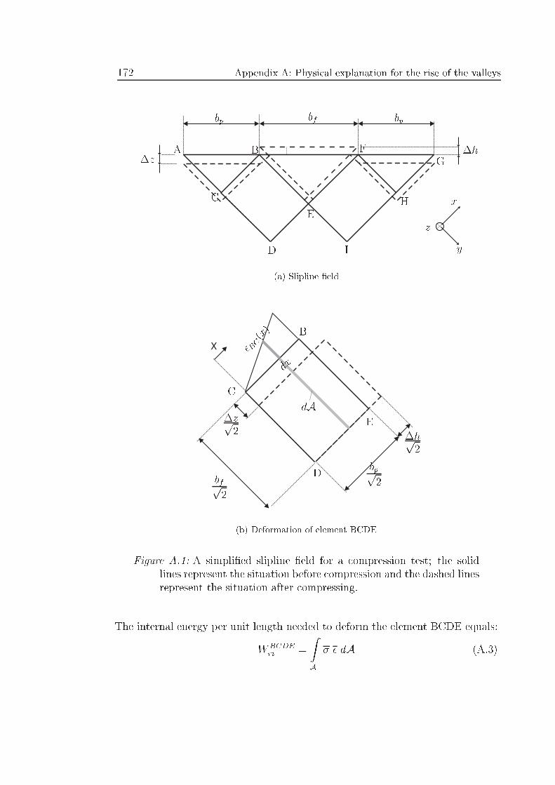
172 Appendix A: Physical explanation for the rise of the valleys
bpbp bf
�z�hA B
C
D
E
FG
H
I
x
y
z
(a) Slipline �eld
xB
C
D
E�zp2
bfp2
bpp2
�hp2
dA
dx
�BC(x)
(b) Deformation of element BCDE
Figure A.1: A simpli�ed slipline �eld for a compression test; the solidlines represent the situation before compression and the dashed linesrepresent the situation after compressing.
The internal energy per unit length needed to deform the element BCDE equals:
WBCDEri =
ZA
� � dA (A.3)
Appendix A: Physical explanation for the rise of the valleys 173
where � is the yield stress �y. � is the equivalent strain and A is the area ofBCDE. � is given by (�xy = 0):
� =
r2
3(�2x + �2y) (A.4)
The strains of BCDE in the x-direction and the y-direction, �x and �y respectively,are given by:
�x =�h
bp(A.5)
and:
�y = ��zbf
(A.6)
The area of BCDE, A, is given by the expression:
A =bfbp2
(A.7)
Because the volume of BCDE remains constant during deformation, �x = ��y.Using this property and combining eqs. (A.3) to (A.7), gives, together with�y = k
p3 (k is the shear strength), for eq. (A.3):
WBCDEri = k�z bp (A.8)
Taking into account deformation of the symmetrical neighbouring element EFHI,the total energy per unit length Wri for deformation is:
Wri = 2k�z bp (A.9)
As is required for a slipline �eld, the external energy given by eq. (A.2) equalsthe internal energy given by eq. (A.9), because, according to Von Misses, p = 2k.Thus, the upper bound criterion (Hu�etink (1998)) is obeyed.
So far, all the applied energy given by eq. (A.2) is assumed to be needed forraising the element BEF by a distance �h. An estimate of the energy absorbedby the element BCDE can be made by assuming shear stresses along the foursides of this element. Assuming a shear stress k along BC, the energy WBC
sh perunit length, absorbed due to shear along BC, becomes:
WBCsh = k
ZA
�BC(x)dA (A.10)
174 Appendix A: Physical explanation for the rise of the valleys
The strain along BC as a function of the distance x, �BC(x), equals (see Fig.A.1(b))
�BC(x) =
p2�h
b2px (A.11)
A small area element dA is given by:
dA =bfp2dx (A.12)
Substituting eq. (A.11) and eq. (A.12) into eq. (A.10) and integrating fromx = 0 to x = bp=
p2 gives:
WBCsh =
1
4k�h bf (A.13)
Because of volume conservation, it can be shown that the absorbed energy perunit length along BE equals eq. (A.13). Taking into account shear along allsides of BCDE and shear along the sides of a second symmetrical neighbouringelement, the total dissipated energy due to shear Wsh per unit length becomes:
Wsh = 2k�h bf (A.14)
Eq. (A.14) represents the energy needed to raise element BEF and is equivalentto eq. (A.9), because �h bf = �z bp.
Concluding, neglecting the in uence of internal material shear, the external en-ergy is entirely totally used for raising the surface (eq. (A.2) equals eq. (A.9)).In this case, making the link with the contact model derived in section 3.2.1, theenergy stored in the asperities, Wintst , is zero (see eq. (3.26)). When the energyneeded for raising the surface is neglected, which implies that Wintri = 0 in eq.(3.26), all the energy is lost to internal shear. When both energy mechanismsplay a role, a fraction � is needed for internal shear and the remaining fraction(1� �) is needed to raise the surface:
Wext = �Wri + (1� �)Wsh (A.15)
with 0 � � � 1. Because Wri = Wsh, eq. (A.15) is obeyed. Therefore, it can beconcluded that the assumptions made in section 3.2.1 are in fact based on realphysical mechanisms.
Appendix B
Expressions for �1, �2, �3 and �
In chapter 3 expressions are needed for the di�erent parameters for the new de-veloped contact model. In this appendix expressions for these parameters will bederived.
Derivation of an expression for �
Eq. (3.25) reads:
�1 =
NPk=1
FNk�zkd�zkFN (B.1)
An expression for �2 is given by eq. (3.29):
�2 =
NPk=1
�zk
Nd�zk (B.2)
From eq. (B.2) follows that:
d�zk =NPk=1
�zk
N�2(B.3)
Substituting eq. (B.3) into eq. (B.1) gives:
�1 =
NPk=1
FNk�zk
FNNPk=1
�zk
N�2 (B.4)
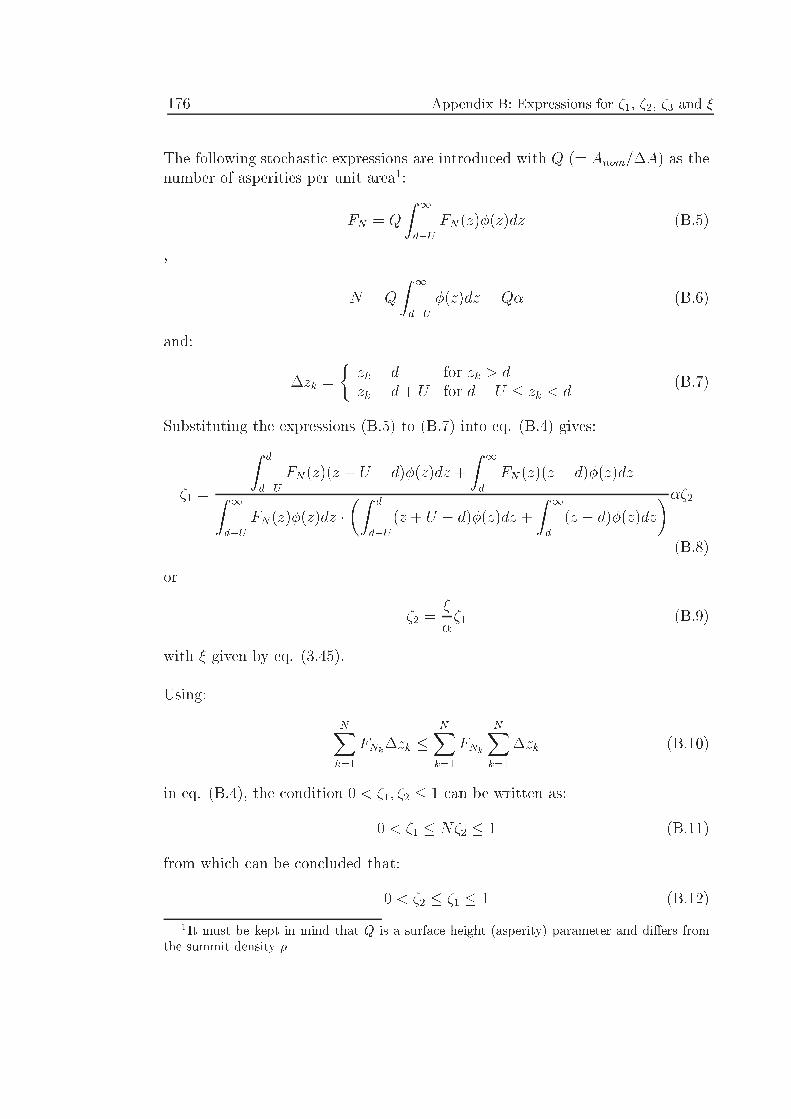
176 Appendix B: Expressions for �1, �2, �3 and �
The following stochastic expressions are introduced with Q (= Anom=�A) as thenumber of asperities per unit area1:
FN = Q
Z 1
d�U
FN(z)�(z)dz (B.5)
,
N = Q
Z 1
d�U
�(z)dz = Q� (B.6)
and:
�zk =
�zk � d for zk > dzk � d+ U for d� U � zk < d
(B.7)
Substituting the expressions (B.5) to (B.7) into eq. (B.4) gives:
�1 =
Z d
d�U
FN(z)(z + U � d)�(z)dz +
Z 1
d
FN (z)(z � d)�(z)dzZ 1
d�U
FN(z)�(z)dz ��Z d
d�U
(z + U � d)�(z)dz +
Z 1
d
(z � d)�(z)dz
���2(B.8)
or
�2 =�
��1 (B.9)
with � given by eq. (3.45).
Using:
NXk=1
FNk�zk �
NXk=1
FNk
NXk=1
�zk (B.10)
in eq. (B.4), the condition 0 < �1; �2 � 1 can be written as:
0 < �1 � N�2 � 1 (B.11)
from which can be concluded that:
0 < �2 � �1 � 1 (B.12)
1It must be kept in mind that Q is a surface height (asperity) parameter and di�ers fromthe summit density �
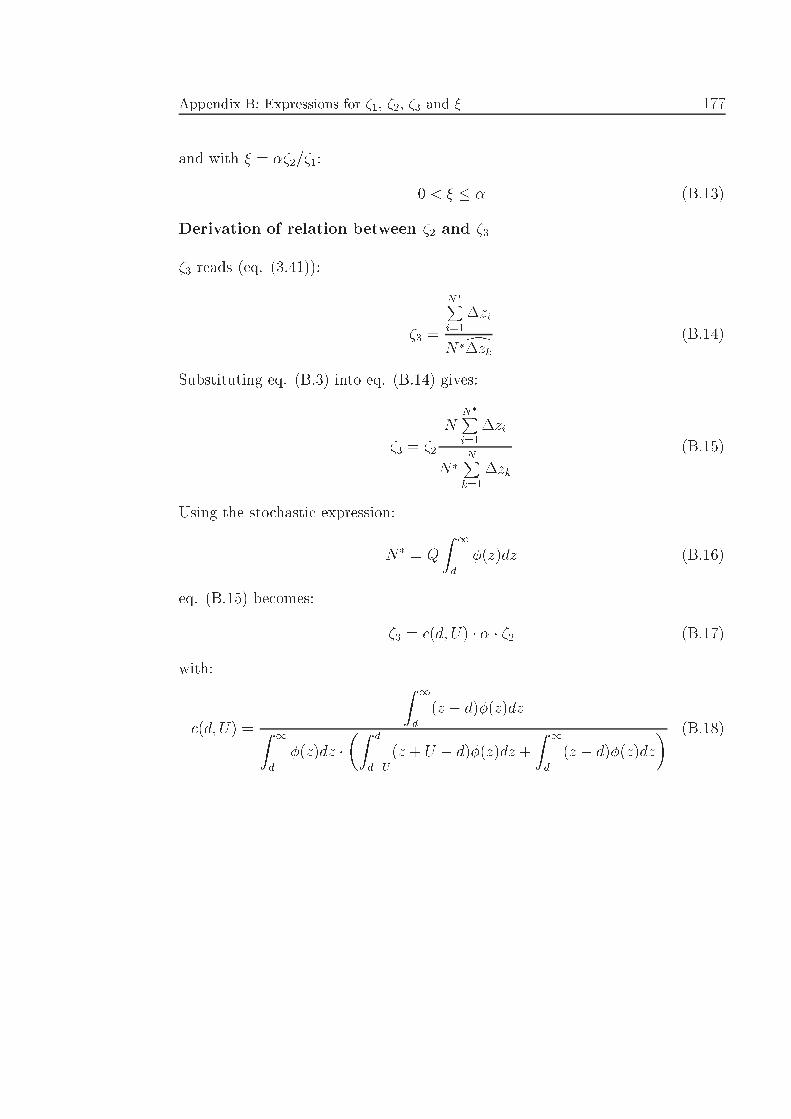
Appendix B: Expressions for �1, �2, �3 and � 177
and with � = ��2=�1:
0 < � � � (B.13)
Derivation of relation between �2 and �3
�3 reads (eq. (3.41)):
�3 =
N�Pi=1
�zi
N�d�zk (B.14)
Substituting eq. (B.3) into eq. (B.14) gives:
�3 = �2
NN�Pi=1
�zi
N�NPk=1
�zk
(B.15)
Using the stochastic expression:
N� = Q
Z 1
d
�(z)dz (B.16)
eq. (B.15) becomes:
�3 = c(d; U) � � � �2 (B.17)
with:
c(d; U) =
Z 1
d
(z � d)�(z)dzZ 1
d
�(z)dz ��Z d
d�U
(z + U � d)�(z)dz +
Z 1
d
(z � d)�(z)dz
� (B.18)

178 Appendix B: Expressions for �1, �2, �3 and �
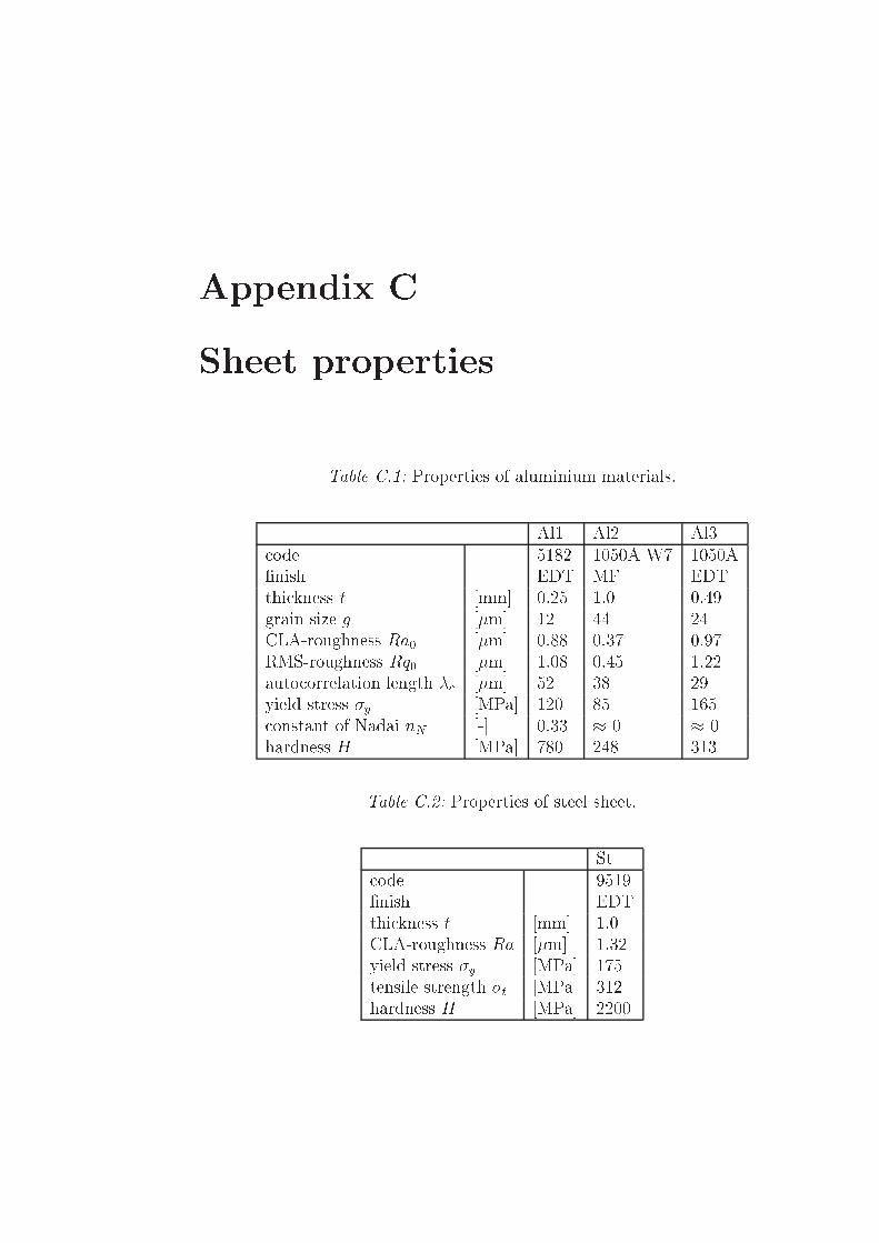
Appendix C
Sheet properties
Table C.1: Properties of aluminium materials.
Al1 Al2 Al3code 5182 1050A W7 1050A�nish EDT MF EDTthickness t [mm] 0.25 1.0 0.49grain size g [�m] 12 44 24CLA-roughness Ra0 [�m] 0.88 0.37 0.97RMS-roughness Rq0 [�m] 1.08 0.45 1.22autocorrelation length �c [�m] 52 38 29yield stress �y [MPa] 120 85 165constant of Nadai nN [-] 0.33 � 0 � 0hardness H [MPa] 780 248 313
Table C.2: Properties of steel sheet.
Stcode 9519�nish EDTthickness t [mm] 1.0CLA-roughness Ra [�m] 1.32yield stress �y [MPa] 175tensile strength �t [MPa] 312hardness H [MPa] 2200

180 Appendix C: Sheet properties
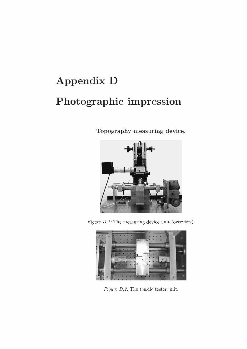
Appendix D
Photographic impression
Topography measuring device.
Figure D.1: The measuring device unit (overview).
Figure D.2: The tensile tester unit.
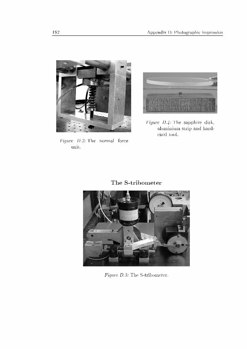
182 Appendix D: Photographic impression
Figure D.3: The normal forceunit.
Figure D.4: The sapphire disk,aluminium strip and hard-ened tool.
The S-tribometer
Figure D.5: The S-tribometer.
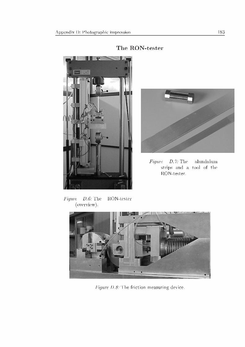
Appendix D: Photographic impression 183
The RON-tester
Figure D.6: The RON-tester(overview).
Figure D.7: The aluminiumstrips and a tool of theRON-tester.
Figure D.8: The friction measuring device.

184 Appendix D: Photographic impression
Bibliography
Abe, T., Shimizu, I. & Nishiyama, T. (1992). Three-Dimensional Observationof Roughening of Free Surfaces During Compressive Plastic Deformation ofPolycrystalline Iron, JSME International Journal 35(4): 462{469.
Adler, R. J. & Firman, D. (1981). A non-Gaussian model for random surfaces,Phil. Trans. R. Soc. London, Series A 303: 433{462.
Akhmatov, A. S. (1966). Molecular Physics of Boundary Lubrication, in D. Davey& Co (eds), Israel Program for Scienti�c Translations, New York.
Atzema, E. H. (2000). Private Communication, Corus RDT.
Bair, S. & Winer, W. O. (1982). Regimes of traction in concentrated contactlubrication, Journal of Lubrication Technology 104: 382{391.
Bassani, R., Di Pasquale, E. & Vitali, C. (1984). Probabilistic model for metal-polymer friction, Wear 95: 177{191.
Bay, N. & Wanheim, T. (1976). Real area of contact between a rough tool and asmooth workpiece at high normal pressures, Wear 38: 225{234.
Bhushan, B. (1984). The real area of contact in polymeric magnetic media - I:Critical assessment of experimental techniques, ASLE Transactions 28: 75{86.
Bigelow, W. C., Pickett, D. L. & Zisman, W. A. (1946). Oleophobic monolayers.I. Films adsorbed from solution in non-polar liquids, Journal of ColloidScience 1: 513{538.
Black, A. J., Kopalinsky, E. M. & Oxley, P. L. B. (1988). An investigation ofthe di�erent regimes of deformation which can occur when a hard wedgeslides over a soft surface: The on uence of wedge angle, lubrication andprior plastic working of the surface, Wear 123: 97{114.
186 Bibliography
Black, A. J., Kopalinsky, E. M. & Oxley, P. L. B. (1990). Sliding metallic frictionwith Boundary Lubrication: An investigation of a simpli�ed friction theoryand of the nature of Boundary Lubrication, Wear 137: 161{174.
Blodgett, K. B. (1935). Films built by depositing successive monomolecular layerson a solid surface, Journal American Chemical Society 57: 1007{1022.
Bowden, F. P. & Leben, L. (1940). The friction of lubricated metals, Phil. Trans.R. Soc. London 239: 1{27.
Bowden, F. P. & Tabor, D. (1954). The Friction and Lubrication of Solids, TheOxford Press.
Bressan, J. D., Genin, G. & Williams, J. A. (1998). The In uence of Pressure,Boundary Films Shear Strength and Elasticity on the Friction Between aHard Asperity and a Deforming Softer Surface, 25th Leeds-Lyon Symposiumon Tribology .
Briscoe, B. J. & Evans, D. C. B. (1982). The shear properties of Langmuir-Blodgett layers, Proc. R. Soc. London, Series A 380: 389{407.
Briscoe, B. J., Scruton, B. & Willis, F. R. (1973). The Shear Strength of ThinLubricant Films, Proc. R. Soc. London, Series A 333: 99{114.
Briscoe, B. J. & Tabor, D. (1973). Rheology of thin organic �lms, ASLE Trans-actions 17(3): 158{165.
Briscoe, B. J. & Tabor, D. (1978). Shear properties of thin polymeric �lms,Journal of Adhesion 9: 145{155.
Campbell, W. E. (1969). Boundary Lubrication, in F. F. Ling, E. E. Klaus &R. S. Fein (eds), Boundary Lubrication: An Appraisal of World Literature,ASME, New York, pp. 87{117.
Carleer, B. (1997). Finite Elements Analysis of Deep Drawing, PhD thesis, Uni-versity of Twente, Enschede, The Netherlands.
Challen, J. M., McLean, L. J. & Oxley, P. L. B. (1984). Plastic Deformationof a Metal Surface in Sliding Contact with a Hard Wedge: Its Relation toFriction and Wear, Proc. R. Soc. London, Series A 394: 161{181.
Challen, J. M. & Oxley, P. L. B. (1979). An explanation of the di�erent regimesof friction and wear using asperity deformation models, Wear 53: 229{243.
Challen, J. M. & Oxley, P. L. B. (1983). Slipline �elds for explaining the me-chanics of polishing and related processes, International Journal MechanicalScience 26(6-8): 403{418.
Bibliography 187
Challen, J. M. & Oxley, P. L. B. (1984). A Slipline Field Analysis of the Transitionfrom Local Asperity Contact to Full Contact in Metallic Sliding Friction,Wear 100: 171{193.
Chang, W., Etsion, I. & Bogy, D. (1987). An elastic plastic model for the contactof rough surfaces, Journal of Tribology 109: 257{263.
Chen, G., Shen, H., Hu, S. & Baudelet, B. (1990). Roughening of the free surfacesof metallic sheets during stretch forming,Materials Science and EngineeringA128: 33{38.
Cheng, H. S., Ling, F. F. & Winer, W. O. (eds) (1973). Mechano-Chemistry inTribology, Proc. NSF Trib. Workshop.
Childs, T. H. C. (1973). The persistence of asperities in indentation experiments,Wear 25: 3{16.
Childs, T. H. C. (1977). The Persistence of Roughness Between Surfaces in StaticContact, Proc. R. Soc. London, Series A 353: 35{53.
Chivers, T. C., Mitchell, L. A. & Rowe, M. D. (1974). The variation of realcontact area between surfaces with contact pressure and material hardness,Wear 28: 171{185.
Dai, Y. Z. & Chiang, F. P. (1992). On the mechanism of plastic deformationinduced surface roughness, Journal of Engineering Materials and Technology114: 432{438.
Dautzenberg, J. H. & Kals, J. A. G. (1985). Surface roughness caused by metalforming, Annals CIRP 34(1): 477{479.
de Rooij, M. B. (1998). Tribological Aspects of Unlubricated Deepdrawing Pro-cesses, PhD thesis, University of Twente, Enschede, The Netherlands.
Demkin, N. B. & Izmailov, V. V. (1975). Plastic contact under high normalpressure, Wear 31: 391{402.
Dowson, D. (ed.) (1994). Friction and Energy Dissipation at the Atomic Scale -a Review, Elsevier, Amsterdam, The Netherlands.
Emmens, W. C. (1997). Tribology of Flat Contacts and its Application in DeepDrawing, PhD thesis, University of Twente, Enschede, The Netherlands.
Gee, M. L., McGuiggan, P. M., Israelachvili, J. N. & Homola, A. M. (1990).Liquid to Solidlike Transitions of Molecularly Thin Films under Shear, J.Chem. Phys. 93(3): 1895{1906.
188 Bibliography
Georges, J. M. & Mazuyer, D. (1991). Pressure e�ects on the shearing of acolloidal thin �lm, Journal Physical Condensed Matter 2: 9545{9550.
Glosli, J. N. & McClelland, G. M. (1993). Molecular dynamics study of slidingfriction of ordered organic monolayers, Physical Review Letters 70(13): 1960{1963.
Godfrey, D. (1968). Boundary Lubrication, P. M. Ku, pp. 335{384.
Granick, S. (1991). Motions and Relaxations of Con�ned Liquids, Science253: 1374{1379.
Greenwood, J. A. (1984). A Uni�ed Theory of Surface Roughness, Proc. R. Soc.London 393: 133{157.
Greenwood, J. A. & Rowe, G. W. (1965). Deformation of surface asperities duringbulk plastic ow, Journal of Applied Physics 36: 667{668.
Greenwood, J. A. & Williamson, J. B. P. (1966). Contact of nominally atsurfaces, Proc. R. Soc. London, Series A 295: 300{319.
Halling, J., Arnell, R. D. & Nuri, K. (1988). Elastic/plastic contact of roughsurfaces and its relevance in the study of wear, Proc. Instn. Mech. Engrs.202(C4): 269{274.
Halling, J. & Nuri, K. (1991). Elastic/plastic contact of surfaces consideringellipsoidal asperities of work-hardening multi-phase materials, Tribology In-ternational 24(5): 311{319.
Hardy, W. & Doubleday, I. (1922). Boundary Lubrication - the ParaÆn Series,Proc. R. Soc. London, Series A 102: 550{574.
Hokkirigawa, K. & Kato, K. (1988). An experimental and theoretical inves-tigation of ploughing, cutting and wedge formation during abrasive wear,Tribology International 21: 51{57.
Homola, A. M., Israelachvili, J. N., McGuiggan, M. & Gee, M. L. (1990). Funda-mental experimental studies in Tribology: the transition from \interfacial"friction of undamaged molecularly smooth surfaces to \normal" friction withwear, Wear 136: 65{83.
Hu�etink, J. (1998). Omvormtechnologie & Plasticiteit En Kruip, University ofTwente, Enschede, The Netherlands. Lecture notes, in Dutch.
Ike, H. & Makinouchi, A. (1990). E�ect of lateral tension and compression onplane strain attening processes of surface asperities lying over a plasticallydeformable bulk, Wear 140: 17{38.
Bibliography 189
Jahanmir, S. & Beltzer, M. (1986). E�ect of additive molecular structure onfriction coeÆcient and adsorption, Journal of Tribology 108: 109{116.
Kasuga, Y., Yamaguchi, K. & Kato, K. (1968). Friction and Lubrication inthe Deformation Processing of Metals (2nd Report, Surface Texture andCoeÆcient of Friction), Bulletin JSME 44: 354{360.
Kimura, Y. & Childs, T. H. C. (1999). Surface asperity deformation underbulk plastic straining conditions, International Journal Mechanical Science41: 283{307.
Komvopoulos, K., Saka, N. & Suh, N. P. (1985). The mechanism of friction inBoundary Lubrication, Journal of Tribology 107: 452{462.
Komvopoulos, K., Saka, N. & Suh, N. P. (1986). The signi�cance of oxide layersin Boundary Lubrication, Journal of Tribology 108: 502{513.
Korzekwa, D. A., Dawson, P. R. & Wilson, W. R. D. (1992). Surface asperitydeformation during sheet forming, International Journal Mechanical Science34(7): 521{539.
Krausz, A. S. & Krausz, K. (1996). Uni�ed Constitutive Laws of Plastic Defor-mation, Academic Press, San Diego, CA., U.S.A.
Landman, U., Luedtke, W. D. & Ringer, E. M. (1992). Molecular DynamicsSimulations of Adhesive Contact Formation and Friction, NATO AdvancedStudy Institutes series 220: 463{510.
Langmuir, I. (1920). The mechanism of the surface phenomena of otation, Trans.Farad. Soc. 15: 62{74.
Lee-Prudhoe, I., Sayler, R. S. & Kaderic, A. (1999). Investigations into asperitypersistence in heavily loaded contacts, Journal of Tribology 121: 441{448.
Lee, W. (1996). Surface Roughening in Metal Forming Processes, PhD thesis,Northwestern University, Evanston, IL, USA.
Liang, X. & Linqing, Z. (1991). A numerical model for the elastic contact ofthree-dimensional real rough durfaces, Wear 148: 91{100.
Liu, G., Wang, Q. & Lin, C. (1999). A survey of current models for simulatingthe contact between rough surfaces, Tribology Transactions 42(3): 581{591.
Lo, S. W. (1999). Surface roughening and contact behaviour in forming of alu-minium sheet, Journal of Tribology 121: 224{233.
190 Bibliography
Lubbinge, H. (1994). Oppervlakte microgeometrie veranderingen ten gevolge vanplaatvervormingsprocessen, Master's thesis, University Twente, Enschede,The Netherlands. in Dutch.
Lubbinge, H., Ter Haar, R. & Schipper, D. J. (1997). The in uence of plasticbulk deformation on surface roughness and frictional behaviour during deepdrawing processes, 22th Leeds-Lyon Symposium on Tribology, Lyon, pp. 705{711.
McFarlane, J. S. & Tabor, D. (1950). Relation between friction and adhesion,Proc. R. Soc. London, Series A 202: 244{252.
Moalic, H., Fitzpatrick, J. A. & Torrance, A. A. (1987). The correlation of thecharacteristics of rough surfaces with their friction coeÆcients, Proc. Instn.Mech. Engrs. 201(c5): 321{329.
Moore, A. J. W. (1948). Deformation of Metals in Static and in Sliding Contacts,Proc. R. Soc. London, Series A 195: 231{249.
Nadai, A. (1927). Plasticity of Materials, Springer, Berlin.
Osakada, K. & Oyane, M. (1971). On the roughening of free surfaces in defor-mation processes, Bulletin JSME 14: 171{177.
Pullen, J. & Williamson, J. P. B. (1972). On the plastic contact of rough surfaces,Proc. R. Soc. London, Series A 327: 159{173.
Ratnager, D. D., Cheng, H. S. & Schey, J. A. (1974). The surface deformationof aluminium compressed with viscous lubricants, Journal of LubricationTechnology 96: 591{594.
Rietman, B. (1999). Numerical Analysis of Inhomogeneous Deformation in PlaneStrain Compression, PhD thesis, University Twente, Enschede, The Nether-lands.
Saha, P. K. & Wilson, W. R. D. (1994). In uence of plastic strain on friction insheet metal forming, Wear 172: 167{173.
Sakurai, T. (1981). Role of chemistry in the lubrication of concentrated contacts,Journal of Tribology 103: 473{485.
Schedin, E. (1991). Micro-Mechanisms of Sheet-Tool Contact in Sheet MetalForming, PhD thesis, Department of Material Technology, Royal Instituteof Technology, Stockholm, Sweden.
Bibliography 191
Schey, J. A. (1983). Tribology in Metalworking - Friction, Lubrication and Wear,ASM, Metals Park, Ohio, USA.
Schipper, D. J. (1988). Transitions in the Lubrication of Concentrated Contacts,PhD thesis, University of Twente, Enschede, The Netherlands.
Shih, H. C. & Wilson, W. R. D. (1999). E�ects of contact pressure and strain onfriction in sheet metal forming, Tribology Transactions 42(1): 144{151.
Sniekers, R. J. J. M. (1996). Friction in Deep Drawing, PhD thesis, EindhovenUniversity of Technology, The Netherlands.
Spikes, H. A. (1989). Additive-additive and additive-surface interactions in lu-brication, Lubrication Science 2(1): 3{23.
Sutcli�e, M. J., Taylor, S. R. & Cameron, A. (1978). Molecular aspects theoryof Boundary Friction, Wear 51: 181{192.
Sutcli�e, M. P. F. (1988). Surface asperity deformation in metal forming pro-cesses, International Journal Mechanical Science 30(11): 847{868.
Tabor, D. (1959). Junction growth in metallic friction, Proc. R. Soc. London,Series A 251: 378{393.
Tabor, D. (1982). The Role of Surface and Intermolecular Forces in Thin FilmLubrication, in J. M. Georges (ed.), Microscopic Aspects of Adhesion andLubrication, Elsevier, Amsterdam, pp. 651{679.
Ter Haar, R. (1996). Friction in Sheet Metal Forming - the In uence of (Local)Contact Conditions and Deformation, PhD thesis, University of Twente,Enschede, The Netherlands.
Thomson, P. F. & Nayak, P. U. (1980). The e�ect of plastic deformation on theroughening of free surfaces of sheet metal, International Journal of MachineTool Design and Research 20: 73{86.
Thomson, P. F. & Shafer, B. V. (1982). The Roughening of Free Surfaces DuringPlasticWorking, International Journal of Machine Tool Design and Research22(4): 261{264.
Timsit, R. S. & Pelow, C. V. (1992a). Shear Strength and Tribological Propertiesof Stearic Acid Films - Part II: On Gold-Coated Glass, Journal of Tribology114: 159{166.
Timsit, R. S. & Pelow, C. V. (1992b). Shear Strength and Tribological Proper-ties of Stearic Acid Films (Part 1) on Glass and Aluminium-Coated Glass,Journal of Tribology 114: 150{158.
192 Bibliography
Torrance, A. A. (1996). The in uence of surface deformation on mechanical wear,Wear 200: 45{54.
Torrance, A. A. (1997). A model of the friction of a smooth hard surface slidingover a softer one, Wear 212: 213{220.
Tsukizoe, T. & Hisakado, T. (1968). On the mechanism of contact betweenmetal surfaces: Part 2 - The real area and the number of the contact points,Journal of Lubrication Technology 90: 81{88.
Uppal, A. H. & Probert, S. D. (1972). Deformation of single and multiple asper-ities on metal surfaces, Wear 20: 381{400.
Uppal, A. H. & Probert, S. D. (1973). The plastic contact between a rough anda at surface, Wear 21: 173{184.
Uppal, A. H., Probert, S. D. & Thomas, T. R. (1972). The real area of contactbetween a rough and a at surface, Wear 22: 163{183.
Van Liempt, P. (1994). Work Hardening and Substructural Geometry of Metals,Journal Material Proceedings Technology 45: 459{464.
Webster, M. N. & Sayles, R. (1986). A numerical model for the elastic frictionlesscontact of real surfaces, Journal of Tribology 108: 314{320.
Wihlborg, A. H. (2000). The In uence of Steel Sheet Surface-Topography on Fric-tion in Stamping, PhD thesis, Chalmers University of Technology, G�oteborg,Sweden.
Williamson, J. B. P. & Hunt, R. T. (1972). Asperity persistence and the realarea of contact between rough surfaces, Proc. R. Soc. London, Series A327: 147{157.
Wilson, W. R. D. (1997). Tribology in sheet metal forming, Proceedings of the1st International Conference on Tribology in Manufacturing Processes, Gifu,Japan, Gifu, Japan, pp. 1{8.
Wilson, W. R. D. & Lee, W. (1997). Mechanics of surface roughening in metalforming processes, Proceedings of the 1st International Conference on Tri-bology in Manufacturing Processes, Gifu, Japan, pp. 71{76.
Wilson, W. R. D. & Sheu, S. (1988). Real area of contact and boundary frictionin metal forming, International Journal Mechanical Science 30(7): 475{489.
Woo, K. L. & Thomas, T. R. (1980). Contact of rough surfaces: a review ofexperimental work, Wear 58: 331{340.
Bibliography 193
Xie, Y. & Williams, J. A. (1996). The prediction of friction and wear when a softsurface slides against a harder rough surface, Wear 196: 21{34.
Zhang, J., Moslehy, F. A. & Rice, S. L. (1991). A model for friction in quasi-steady-state sliding Part I. derivation, Wear 149: 1{12.