Modelling of an Electroactive Polymer Actuator

Procedia Engineering 48 ( 2012 ) 1 – 9

1877-7058 © 2012 Published by Elsevier Ltd.Selection and/or peer-review under responsibility of the Branch Offi ce of Slovak Metallurgical Society at Faculty of Metallurgy and Faculty of Mechanical Engineering, Technical University of Košicedoi: 10.1016/j.proeng.2012.09.477

MMaMS 2012

Modelling of an electroactive polymer actuator

Ákos Aczéla* aSzéchenyi István University, Egyetem tér 1,Gy r, H-9026, Hungary

Abstract

The aim of this paper is to build a model of an electroactive polymer actuator when external electric field is applied. Materials whose rheological properties can be varied by electric excitation are called electroactive materials. The behavior of these rubberlike media is commonly investigated in two different ways. Brigadnov, Dorfmann, Bustamante, Ogden and others describe the coupled problem of finite deformation of the continua in electromagnetic field by taking into account all the electromagnetic phenomena. Pelrine, Kornbluh, Sommer-Larsen and others present a phenomenological description. Our aim is to form a bridge between these two points of view by neglecting those terms of the governing and transformation equations that are smaller than other contributions by several orders of magnitude. First, those equations are presented that govern the finite deformation and the electromagnetic phenomena inside the material. After that, those estimations will be taken that show the order of magnitude of the different contributions to the so-called effective fields. Finally, the model of the EAP actuator under periodically changing electric field will be presented. Because of the periodically changing finite deformation of the actuator, the electromagnetic phenomena must be investigated in the rest frames fixed to every single point of the material body. The electromagnetic field-variables can be converted into the laboratory frame by the slow speed approximation of the Lorentz transformation. For the special case of thin electroactive polymer actuators, one can find that the velocity dependent contributions are smaller by ten orders of magnitude in the electric field transformation, and by five orders of magnitude in the magnetic field transformation equations. On the other hand, none of the terms of the effective current can be neglected, because they can be of the same order of magnitude as the free current. © 2012 The Authors. Published by Elsevier Ltd.

Selection and/or peer-review under responsibility of the Branch Office of Slovak Metallurgical Society at Faculty of Metallurgy and Faculty of Mechanical Engineering, Technical University of Košice.

Keywords: electroactive polymer actuator, effective field, Lorentz transformation, constitutive equation

Nomenclature

c speed of light in the vacuum (m/s) d thickness of the EAP layer (m) f frequency (1/s)

q charge per unit volume (C/m3)

A area of the EAP layer (m2) C capacitance of the EAP actuator (F) F force acting on the EAP layer due to the applied voltage (N) I current (A) U potential energy per unit volume (J/m3) Y Young’s modulus (N/m2) V voltage applied to the actuator (V)

* Corresponding author. E-mail address: [email protected].

Available online at www.sciencedirect.com

© 2012 Published by Elsevier Ltd.Selection and/or peer-review under responsibility of the Branch Offi ce of Slovak Metallurgical Society at Faculty of Metallurgy and Faculty of Mechanical Engineering, Technical University of Košice

2 Ákos Aczél / Procedia Engineering 48 ( 2012 ) 1 – 9

r position vector (m) ( )nt stress vector (traction) at the surface with unit normal n (N/m2)

v velocity of the material body (m/s) B magnetic induction (T) D electric displacement (C/m2) E electric field intensity (V/m) F force per unit volume, acting on the material body (N/m3) H magnetic field intensity (A/m) J current per unit area (A/m2) L body couple per unit volume (N/m2) M magnetization density (A/m) P polarization density (C/m2) Q heat flux vector (W/m2) Greek symbols

0,rε ε relative dielectric constant, dielectric constant in the vacuum (1, As/Vm)

0,rμ μ relative magnetic permeability, magnetic permeability in the vacuum (1, Vs/Am)

ν conductivity (A/Vm) ρ mass density (kg/m3)

Φ energy supply density (W/m3) Vector calculus

⋅a b scalar product (dot product) of two vectors ×a b vector product (cross product) of two vectors

∇ Nabla, Hamilton’s differential operator

curlE ( ), ijk j kicurl Eε∇× = ∂E E

divE , i iE∇ ⋅ ∂E

V

dVa volume integral of a over the volume V

S

da S surface integral of a over the surface S

C

da C contour integral of a over the curve C

S

da S flux of a on the surface S

1. Introduction

The electroactive materials can deform in response to applied electric fields. Therefore, the actuators made from these rubberlike materials have been a promising area of research for more than a decade now [1-2]. Pelrine, Kornbluh, Sommer-Larsen and others have presented a phenomenological description by summarizing and interpreting countless results in measuring [3]. Unfortunately, there are several difficulties when modeling these rubberlike materials under finite deformations while excited by electric field. Brigadnov, Dorfmann, Bustamante, Ogden and others describe this coupled problem of finite deformation of the continua in electromagnetic field by taking into account all the electromagnetic phenomena [4-6]. In general, it is the perfect method for describing all the electromagnetic phenomena. But in some cases, especially, when no external magnetic field emerges, and the material body under investigation is flat, some effects can be disregarded.

2. The balance equations

The mechanical behavior of any material body is governed by the balance equations of the continuum mechanics [7]. These four basic balance laws are:

Balance of mass:


0V

ddV

dtρ = (1)

Balance of linear momentum:

( )

V S V

ddV dS dV

dtρ = +nv t F (2)

Balance of angular momentum:

( )

V S V

ddV dS dV

dtρ× = × + × +nr v r t r F L (3)

Balance of energy:

( )( ) ( )1

2 Q

V S V

dU dV dS dV

dtρ ⋅ + = ⋅ − ⋅ + ⋅ + Φ + Φnv v t v Q n F v (4)

The question is what functions appear as body force per unit volume F , body couple per unit volume L , and energy supply density Φ of electromagnetic origin. Naturally, all these three functions can be derived from the electromagnetic field variables. Unfortunately, the body force, the body couple and the energy supply can be variedly postulated according to the formulation used to describe the electromagnetic phenomena in the moving media [8-9].

3. The Maxwell-equations for media in rest

In vacuum, the physical laws for the electromagnetic field-variables are the well-known Maxwell-equations [10]:

curlt

∂= +∂D

H J (5)

curlt

∂= −∂B

E (6)

div 0=B (7)

div q=D (8)

These local equations can be derived from the global Maxwell-equations: Ampère–Maxwell

C S S

dd d d

dt⋅ = ⋅ + ⋅H C J S D S (9)

Faraday

C S

dd d

dt⋅ = − ⋅E C B S (10)

Gauss–Faraday


0S

d⋅ =B S (11)

Gauss–Coulomb

S V

d q dV⋅ =D S (12)

Since these integrals can be measured, only the global laws can be proven by experiments. In the vacuum 0ε=D E and

0μ=B H , so two field variables are sufficient for describing all electromagnetic phenomena, one for electric and one for

magnetic fields. The sources of the electric and magnetic fields are electric charge and electric current, respectively. For material bodies, the relationships between the field variables (and the current) can be very complex:

( ) ( ) ( ), ; , ; ,= = =D E H B H E J E H (13)

where ; ; are general vector functions. These equations are often called as the constitutive equations for the

material under discussion. For linear isotropic materials the constitutive equations are:

; ; ,ε μ ν= = =D E B H J E (14)

where ε is called the dielectric constant, μ the magnetic permeability, and ν the electric conductivity. There is a

tendency to regard E and B fields as the basic variables for electric and magnetic fields in the vacuum so the constitutive laws can be rewritten by introducing two more variables for material media:

( )0 0; ,ε μ= =D E P B H M+ + (15)

where P is the polarization density and M is the magnetization density. Their definitions are the above two equations.

4. The equations for moving media

In the case of moving media, the first challenge is to find the adequate reference co-ordinate system. The laboratory frame is regarded as inertial system and the intensity of the external electromagnetic field is usually given in this representation, so it seems obvious to describe all the electromagnetic phenomena in the laboratory frame.

Unfortunately, the constitutive equations are known only for the material lying at rest. In addition, all the points of the deforming media may move by the velocity of their own, so there is no co-ordinate system in which the material body under investigation seems to be at rest. Naturally, one can choose a co-ordinate system in which one single point and its small surroundings are at rest and this system may be called rest frame (Fig. 1.). However, other areas of the body under investigation may not be at rest according to this so-called rest frame.

x

y

z

x′ y′

z′

E H

v

Laboratory

frame

Rest frameMoving media

v

Fig. 1. Laboratory frame and rest frame for describing the moving media


The first step of the usually chosen procedure is to write and solve the Maxwell-equations in all the co-ordinate systems fixed to every single point of the moving and deforming media. After that, the results must be converted into the laboratory frame. The Achilles heel of this method is the transformation from one co-ordinate system to an other. Coordinates of the electromagnetic variables must be transformed from one system to the other according to the Lorentz transformation. As the velocity is much smaller than the speed of light, the slow speed approximation of the Lorentz transformation can be used:

2c′ ′= × ×E E v B D D v H+ ; = + (16)

2c′ ′− × = − ×H H v D B B v E= ; (17)

2q q q c′ ′= − = −J J v v J; (18)

The use of these transformation equations is self-evident in vacuum, but there are different commonly used formulations for transformation in the presence of matter. Some of these formulations are discussed in [8]. It is important to note that they differ from each other not only in some notations but also in regarding the polarization and the magnetization relevant or irrelevant when defining the effective fields.

The use of Lorentz transformation is problematic in other respect as well: The points of the deforming material body are moving with not a constant velocity, and no co-ordinate system fixed to an accelerating point can be rigorously considered as inertial system. On the other hand, the acceleration can be managed by postulating inertial forces and the relativistic effects can surely be neglected since the velocities are very small, compared to the speed of light.

Further problems emerge when taking into account the electromagnetic effects of the moving charged particles of the deforming material itself [11-12]. Fortunately, in the case of electroactive polymer (EAP) actuators no charged particles and no current occur inside the material.

5. The model of the EAP actuator

The geometry of the common EAP actuators is planar or can be considered planar (the thickness is much smaller than the curvature of the device). The mechanical model of an average EAP actuator (Fig. 2.) can be imagined as a flat capacitor: a thin electroactive polymer layer coated on both side with compliant conductive film (these are the plates of the capacitor and are said to be compliant because they can strain together with the polymer even under finite deformation). The polymer is rubberlike and quasi-incompressible with a Young’s modulus of some MPa. Actuation is caused by electrostatic force between the two electrodes (Maxwell pressure). This force squeezes the polymer and because of its quasi-incompressibility, it expands in area due to the electric field. Therefore, charge and current can occur only on the surface, or more precisely in the plates of the capacitor.

( ) ( )max maxsin 2V t V f tπ=

EAP layer

complient

conductive films

30 md =

Fig. 2. Model of the EAP actuator

The EAPs are excellent insulators so no free charge and no free current can occur inside the material, except for the case of damage [3] There is a lack of magnetisable particles in the EAPs, too. These facts simplify the Maxwell equations:


0curlt t

ε ∂ ∂= +∂ ∂E P

H (19)

curlt

∂= −∂H

E (20)

div 0=H (21)

0div divε= −P E (22)

The polarization is observed to be the function of the electric field intensity, the temperature and the stretch [13]. Hysteresis may also occur so the constitutive equation is evidently nonlinear [14]. In addition, we can assume the lack of external magnetic field as the EAP actuators are usually used without external magnetic excitation. Unfortunately, it does not mean that no magnetic phenomena would take place at all. When an EAP actuator is in steady state (that is to say there is no more change in its dimensions and electric field intensity inside), it is self evident that no current is flowing, so no magnetic field emerges. However, before reaching the steady state the shape of the actuator changes in time, so the charge on the plates moves together with the EAP’s surface. It means current from the point of view of those who are in the laboratory frame, this current results in magnetic field, according to the Ampère–Maxwell law. Although the current is outside the material body under survey, the magnetic field caused by this current will affect the whole EAP actuator. Furthermore, we have to face the problem of the different co-ordinate systems because of the movement of the media.

6. Electromagnetic and mechanical conditions in the EAP actuators

The EAP film thickness can vary from several m up to some ten m, depending on the original thickness of the film and the prestretch. The maximum electric field strength can be more than 108 V/m [13]. It results in a breakdown voltage of some kV. The capacitance and the capacitive energy can be calculated by the well-known formulae:

2 20 0

1 1;

2 2r C r

A AC E V C V

d dε ε ε ε= = = , (23)

where rε relative dielectric constant can vary between 3 and 5 depending on the material, the electric field intensity and the stretch. The force, what an actuator of this type can exert is:

20

2C rdE V A

Fdd d

ε ε= = − (24)

The incompressibility of the material has been taken into account due to the Ad=const. condition. This force is perpendicular to the capacitor’s plate and results in compressing the polymer in thickness.

The external electric field is sinusoidal. The higher the frequency is, the more significant magnetic phenomena are expected. However, there is no mean in increasing it above the usual operating frequency. According to the experiments [3] (page 118), some kHz is available as a maximum operating frequency. Assuming that the voltage applied on the device is sinusoidal and the capacitance does not change in time, the current is sinusoidal also.

( )( ) 2 cos 2I t f CV f tπ π= (25)

This current causes a magnetic field inside the polymer.

( )0

2 cos 2;

f CV f tIH B H

A A

π πμ= = = (26)


( )V t

J B

BJ

Fig. 3. Magnetic induction due to the current flowing into the plate of the capacitor

For the sake of simplicity, the shape of the capacitor is assumed as square. The field intensity is parallel with the conductive layers and perpendicular to the direction of the current (Fig. 3.).

In addition, a magnetic field is induced due to the altering electric displacement. It equals:

( )00

2cos 2 ;

4 4r

D f VtH f t B HA A d

π ε ε π μ∂

∂′ ′ ′= = =⋅

(27)

This contribution to the magnetic field is also parallel with the layers and reaches its highest amount near the edges of the EAP layer (Figure 4.).

( )V tD

′B

Fig. 4. Magnetic induction due to the change of the electric displacement

The above calculations were all made under the assumption that there are no movements in the system. The EAP is considered incompressible, therefore the change of area due to the applied voltage is:

FA

YΔ = − (28)

Changing in area goes hand in hand with the acceleration and velocity of every single point in the material body. The maximum speed occurs at the edges of the actuator:

20

max 24

4r

A V AFv f f f

d YA Y A

ε επ π πΔ

= = = (29)

It can increase up to some m/s [9]. With these results, one can estimate the ratios of the terms in the Lorentz transformation:

2

0 0

2rV f

Y d

μ ε ε π×=

v B

E(30)

2

02 2

r V f

Y dcc

ε ε π×=

v H

D(31)

20

2

2 rV A

d Y

ε ε×=

v D

H(32)


2

2 2 20

2V A

c d Yc μ×

=v E

B(33)

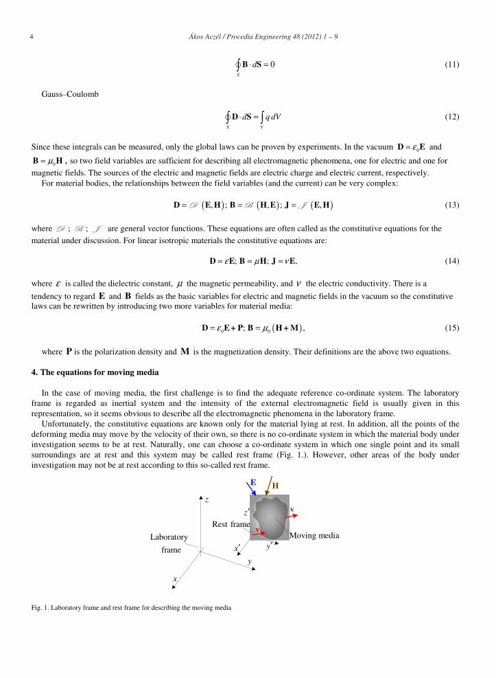
Substituting the abovementioned maximum operational frequency and breakdown voltage, the first two ratios happen to be of the order of 10-10, the third and fourth ones of the order of 10-5.

After these calculations, we can get back to the main question: “what functions appear as body force per unit volume F , body couple per unit volume L , and energy supply density Φ of electromagnetic origin” in the balance equations of the continuum mechanics. Body couple equals zero, as no magnetisable parts can be found in the material. The abovementioned formulations agree in the expression called Maxwell-Lorentz force and the energy supply expression [6]:

tq= + ×tF E J B (34)

tΦ = ⋅J E (35)

tq q= − ∇ ⋅ P (36)

( )t t

∂= + + ∇ × × + ∇ ×∂P

J J P v M (37)

The only difference between the formulations is that the ( )∇× ×P v term is missing in the Maxwell formulation. The polarization field is homogenous inside the EAP, therefore its divergence equals zero. In addition, no magnetization takes place at all. Only two terms remained in the expression of the total current density.

( ) 01 2r

Vf

t dε ε π∂ = −

∂P

(38)

Substituting the breakdown voltage and the maximum frequency, and then multiplying by the area of the actuator, one can get a current comparable with the free current flowing into the electrodes. Polarization is assumed homogenous inside the material, but velocity is linearly changing from one edge of the actuator to the opposite. Taking notice of only linear dislocation:

( ) ( )3

2max max0 3max

1r r

P v Vcurl f

d YAε ε ε π× = = −P v (39)

It happens to be some percent of the free current. This term emerges only in the Lorentz formulation so this fact can be a basis for deciding by experiments which formulation describes the real electromagnetic phenomena in the moving media. Finally, the current due to the movement of the charged electrodes can be estimated as:

3 32 2 max

max max max 0 max3r

V AI CV v f

d Yε ε π′ = = (40)

It is smaller than the free current by five orders of magnitude.

7. Conclusions

Before deciding which term to neglect, one has to take into account that the experimental data of the constitutive equations show high variation. The material properties of the EAPs change with frequency, temperature, stretch, and even in time. In these circumstances, it is useless to take into account negligible effects. The calculations of the last section showed us which terms could be neglected in the (16-18) formulae of the Lorentz transformation and in the (36-37) formulae of the total charge and total current density. According to (30-33), the ×v B and the 2c×v H terms can surely be disregarded. Although ×v D and 2c×v E play a role higher by five orders of magnitude, they can be neglected too. All results depend


on the working frequency, the relative dielectric constant, the maximum voltage and the thickness of the EAP layer. These can vary due to technological development; therefore, the estimations must be repeated if better materials are achieved.

The current due to the movement of the charged electrodes is negligible compared to the free current measured in the rest frame (40). Therefore, it does not have to be taken into account at all.

The polarisation current and the free current are of the same order of magnitude, so none of them can be neglected. The ( )curl ×P v term could be estimated as some percent of the polarisation current, so it cannot be disregarded either.

Acknowledgements

The research was supported by the Project BAROSS-ND07-ND-INRG5-07-2008-0062.

References

[1] Carlson, J. D., Jolly, M. R., 2000. MR Fluid, Foam and Elastomer Devices, Mechatronics, 10, pp. 555-569. [2] Kordonsky, W., 1993., Magnetorheological Effects as a Base of New Devices and Technologies, Journal of Magnetism and Magnetic Materials, 122,

pp. 395-398. [3] Carpi, F. et al., 2008. Dielectric Elastomers as Electromechanical Transducers, Elsevier [4] Brigadnov, I. A., Dorfmann, A., 2003. Mathematical Modelling of Magneto-sensitive Elastomers, International Journal of Solids and Structures, 40, pp.

4659-4674. [5] Bustamante, R., Dorfmann, A., Ogden, R. W., 2009. On Electric Body Forces and Maxwell Stresses in Nonlinearly Electroelastic Solids, International

Journal of Engineering Science, 47, pp. 1131-1141. [6] Dorfmann, A., Ogden, R. W., 2004. Nonlinear Magnetoelastic Deformations of Elastomers, Acta Mechanica, 167, pp. 13-28. [7] Maugin, G. A., 1988., Continuum Mechanics of Electromagnetic Solids, North-Holland, Amsterdam, pp. 95-117. [8] Pao, Y. H., 1978., Electromagnetic Forces in Deformable Continua, in: Mechanics Today, 4., Nemat-Nasser, S., Editor. Pergamon Press, pp. 209-306. [9] Aczél, Á., 2012. Electromagnetic Forces in Electroactive Polymers, Acta Technica Jaurinensis 5/1, pp. 87-101. [10] Kuczmann, M., Iványi, A., 2008., The Finite Element Method in Magnetics, Akadémiai Kiadó, Budapest [11] Jolly, M. R., Carlson, J. D., Munoz, B. C., 1996., A Model of the Behaviour of Magnetorheological Materials, Smart Materials and Structures, 5, pp.

607-613. [12] Bradshaw, D. H et al., 2010. Electromagnetic Momenta and Forces in Dispersive Dielectric Media, Optics Communications 283, pp. 650-656. [13] Kofod, G. et al., 2003. Actuation response of polyacrylate dielectric elastomers, Journal of Intelligent Material Systems and Structures 14/12, pp. 787-

793 [14] Vu, D. K., Steinmann, P., 2007., Nonlinear Electro- and Magneto-elastics: Material and spatial settings, International Journal of Solids and Structures,

44, pp. 7891-7905.

Documents

Modelling of an Electroactive Polymer Actuator