Journal of Sound and Vibration (1995) 184(3), 503–528

MODELLING OF A HYDRAULIC ENGINE MOUNTFOCUSING ON RESPONSE TO SINUSOIDAL AND

COMPOSITE EXCITATIONS

J. E. C, C.-T. C, Y.-C. C, W. K. L L. M. K

Department of Mechanical Engineering, Northwestern University, Evanston,Illinois 60208, U.S.A.

(Received 14 June 1993, and in final form 24 June 1994)

Frequency response characteristics of a hydraulic engine mount are investigated.The mount studied is highly non-linear due to an amplitude-limited floating piston (the‘‘decoupler’’) which enables the response to large amplitude (typically road-induced)excitations to differ markedly from the response to small amplitude (typically engine-induced) excitations. The effect of the decoupler on frequency response as well ascomposite-input (sum of two sinusoids) response is considered.

New experimental data for a production mount and several specially prepared mountsare presented and discussed. Two linear models, one for large amplitude excitationsand one for small amplitude excitations, are developed and shown to be effective over a5–200 Hz frequency range. The latter model explains a moderately high frequency(0120 Hz) resonance which is often observed in the data, but which has not previouslybeen described in physical terms.

A piecewise linear simulation and an equivalent linearization technique are used toexplain the amplitude-dependence of frequency response, as well as the composite-inputresponse. The applicability of equivalent linearization is justified by demonstrating thathigh order harmonics contribute very little to the transmitted force. Moreover, thistechnique is found to be computationally efficient and to provide insight into decouplerdynamics.

7 1995 Academic Press Limited

1. INTRODUCTION

Engine mounts serve two principal functions: vibration isolation and engine support.In the past decade, the automotive industry’s shift to small, four cylinder engines andtransversely mounted front-wheel-drive powertrains has made these two functions increas-ingly incompatible. For instance, the lower firing frequencies of four cylinder enginescoupled with lower engine inertia tend to excite higher amplitude vibrations. To avoidsignificant chassis vibration and passenger compartment noise, softer mounts becomenecessary—it is not uncommon for the elastic rate (stiffness) of a mount in a front-wheel-drive automobile to be 20 times less than that of a rear-wheel-drive automobile [1]. Enginemounts, however, must also limit or ‘‘control’’ engine excursions caused by rough roads,idle shake, vehicle accelerations and wheel torque reaction (which is especially an issue infront-wheel-drive). To provide control, it is important that the engine mounts be stiff andheavily damped. This growing disparity between isolation characteristics and controlcharacteristics has profoundly changed the way in which the industry approaches mountdesign.

503

0022–460X/95/280503+26 $12.00/0 7 1995 Academic Press Limited

. . .504

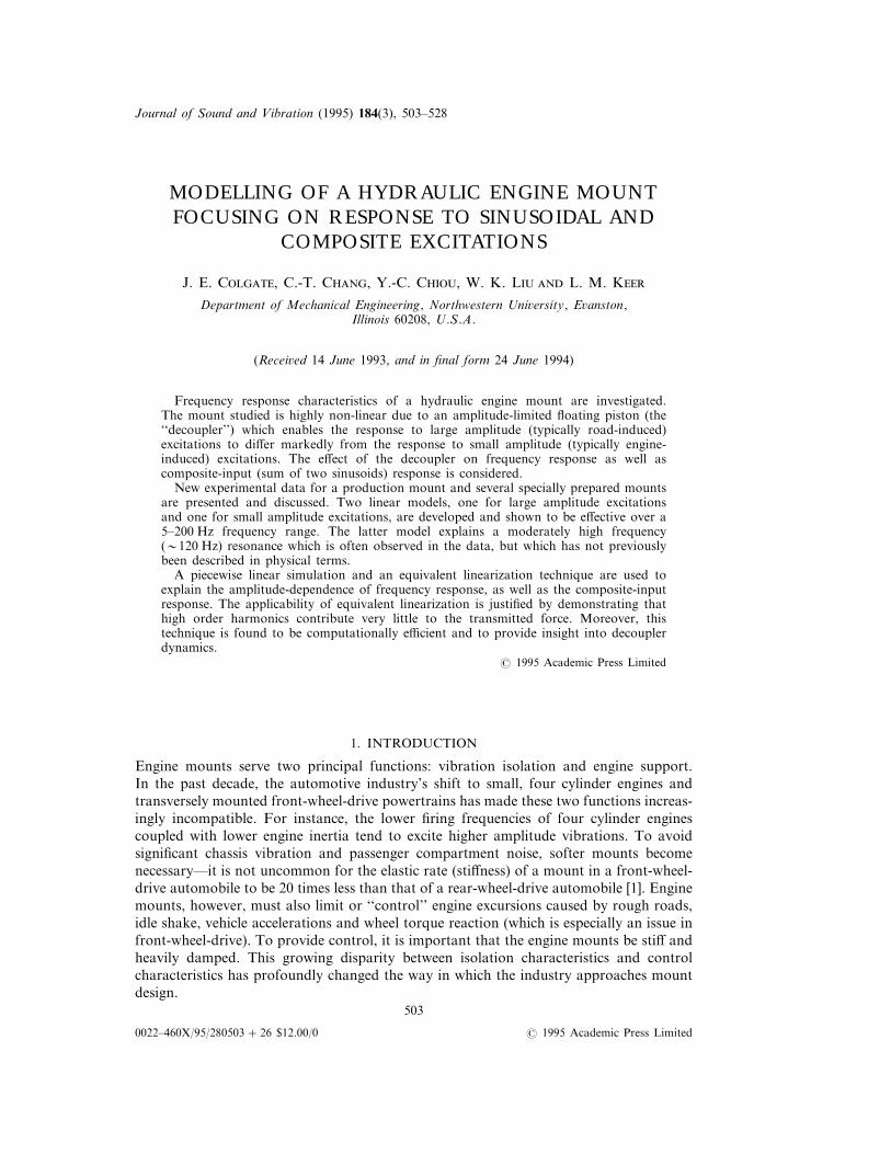
Figure 1. A schematic of a hydraulic engine mount.

Change has also been forced by an increased market emphasis on passenger comfort.Comfort encompasses interior noise and vibration as well as the feel of the vehicle on roughroads and under extreme acceleration. This serves only to heighten the conflicts that arisein design.

To meet the conflicting requirements of isolation and control, the automotive industryhas turned increasingly to hydraulic engine mounts. A typical hydraulic mount isillustrated in Figure 1. To provide a basis for the design and analysis of such a mount,good models are essential. Toward this end, a variety of articles presenting mathematicalmodels as well as design procedures has been published in the past decade [2–15].An excellent review is provided by Singh et al. [11]. It should be noted that, while thispaper focuses on passive engine mounts, a number of recent studies have exploredsemi-active or adaptive engine mounts as well [3, 10, 16–18].

Until recently, most attempts to model hydraulic mounts assumed linearity and wererestricted to rather limited sets of operating conditions (usually corresponding to testconditions). Unfortunately, production hydraulic mounts exhibit a variety of non-linearcharacteristics and, in application, are subject to a broad range of excitations. Theinvestigation of non-linear behavior appears to have begun with Ushijima and Dan [13],who used numerical simulation to investigate nonlinear flow characteristics. More recently,Kim and Singh [19, 20] began a systematic study of hydraulic mount non-linearities.Among the effects they have considered are non-linear compliance, non-linear flowcharacteristics, cavitation and ‘‘decoupling’’.

This paper contributes further to the understanding of mount non-linearity associatedwith the ‘‘decoupler’’. The decoupler, shown in Figure 1, is essentially an amplitude-dependent switch which is intended to improve the performance trade-off betweenvibration isolation and control of engine excursion.

Other contributions of this paper include the presentation of new experimental datadescribing the response of a hydraulic mount to composite, dual frequency excitations, aswell as the presentation of a novel ‘‘small amplitude linear model’’. This linear model,developed as a preliminary to non-linear models, is the first in the literature to capture animportant resonance associated with decoupler inertia. All models presented in this paperconsider single axis excitation only, though extension to multiple axes is possible.

505

2. HYDRAULIC ENGINE MOUNT CHARACTERISTICS

2.1.

In Figure 1, xe (t) and xc (t) represent the displacement of the engine and thechassis, respectively. The relative displacement, x0(t)= xe (t)− xc (t), is referred to asthe ‘‘excitation’’ of the moment. Physical components which contribute significantly to thedynamics of the mount include the following. The primary rubber (1) is a rubber cone thatserves several purposes. It support the static load of the engine, it contributes (significantly)to the elastic rate and (modestly) to the damping of the mount and it serves as a pistonto pump fluid through the rest of the mount. The bulge rate of the primary rubber (ratioof pressure change to volume change) is also an important design parameter. Thesecondary rubber (2) is a rubber septum that serves principally to contain the fluid. It alsocontributes modestly to the elastic rate. The orifice plate (3) is a metal plate (actually asandwich of two plates) that separates the ‘‘upper chamber’’ (enclosed by the primaryrubber) and the ‘‘lower chamber’’ (enclosed by the secondary rubber). Cast in the orificeplate are the ‘‘inertia track’’ and ‘‘decoupler orifice.’’ The inertia track (4) is a lengthy spiralchannel that enables fluid to pass from the upper chamber to the lower chamber. The fluidinertia in this channel is significant, and is usually selected so that it experiences resonanceat the natural frequency of the engine/mount system. The damping of the track is alsosignificant. Thus, the inertia track acts as a tuned damper, and is introduced for thepurpose of control. The decoupler (5) is a plastic plate which acts as an amplitude-limitedfloating piston that provides a low resistance path between the upper and lower chambers.Thus, for small amplitude excitation, most of the fluid transport between chambers is viathe decoupler orifice, which effectively short-circuits the inertia track. For larger amplitudeexcitations, the decoupler ‘‘bottoms out’’ and most of the fluid flow is forced through theinertia track. The inertia of the decoupler is also important at high frequencies, a pointwhich will be highlighted in this paper. The fluid (6), ethylene glycol, completely fills theinterior of the mount.

2.2.

The behavior of an engine mount is usually reported in terms of its frequency responsefor different amplitude excitations. Frequency/amplitude ranges of greatest interestinclude [6, 11, 14]: (1) 5–15 Hz, 0.5–5.0 mm—these excitations are in the range of engineresonance and large enough to require significant damping; (2) 25–250 Hz, 0.05–0.5 mm—these excitations can cause noise and vibration, and require good isolation. Even higherfrequency excitations, which may result from combustion noise [14], have receivedattention recently, but are beyond the scope of this paper. Interest has also arisen in theextent to which hydraulic mounts can provide control and isolation simultaneously [14].This may be important, for instance, while driving on rough surfaces, or during extremeaccelerations on smooth surfaces. Thus, the response to composite inputs is of interest, andwill be considered in this paper.

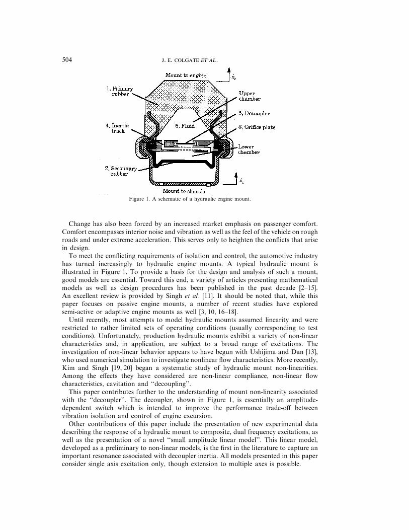
The frequency response is typically evaluated with a conventional servo-controlledhydraulic test rig. The chassis bracket is fixed to an inertially grounded force sensor, whilethe engine bracket is sinusoidally excited at a fixed amplitude. Force and displacementrecords are collected at a series of frequencies and each record is transformed to thefrequency domain via a discrete Fourier transform. For this study, time domain recordsall consist of 8192 points collected at a sample interval of 0·0005 s. To analyze highfrequency behavior (5–200 Hz increments), each record is broken into four contiguoussections which are independently windowed (Hanning window) and transformed. The fourtransforms are then ensemble-averaged to obtain estimates of the Fourier transform

. . .506

and coherence. To analyze low frequency behavior (1–40 Hz in 1 Hz increments), eachrecord is broken into eight interleaved sections (each with an effective sample rate of0.004 s), which are independently windowed and transformed, then ensemble-averaged.†In all cases, only those data corresponding to the excitation frequency, v, are retained.Coherences obtained in this way are not reported because they are in all cases extremelyclose to unity. The Fourier transforms, F( jv) and X0( jv), correspond to the fundamentalharmonics of force and displacement. The ratio of these transforms, known as the‘‘dynamic stiffness’’ is the principal quantity of interest:

Kdyn ( jv)=F( jv)/X0( jv)=K(v)+ jvB(v). (1)

The real part of the dynamic stiffness, K(v), is termed the ‘‘elastic rate’’, while theimaginary part divided by frequency, B(v), is termed the ‘‘damping’’. In comparing thesedata with others in the literature, it should be noted that dynamic stiffness is oftenpresented in terms of the magnitude (‘‘dynamic rate’’) and phase (‘‘loss angle’’).

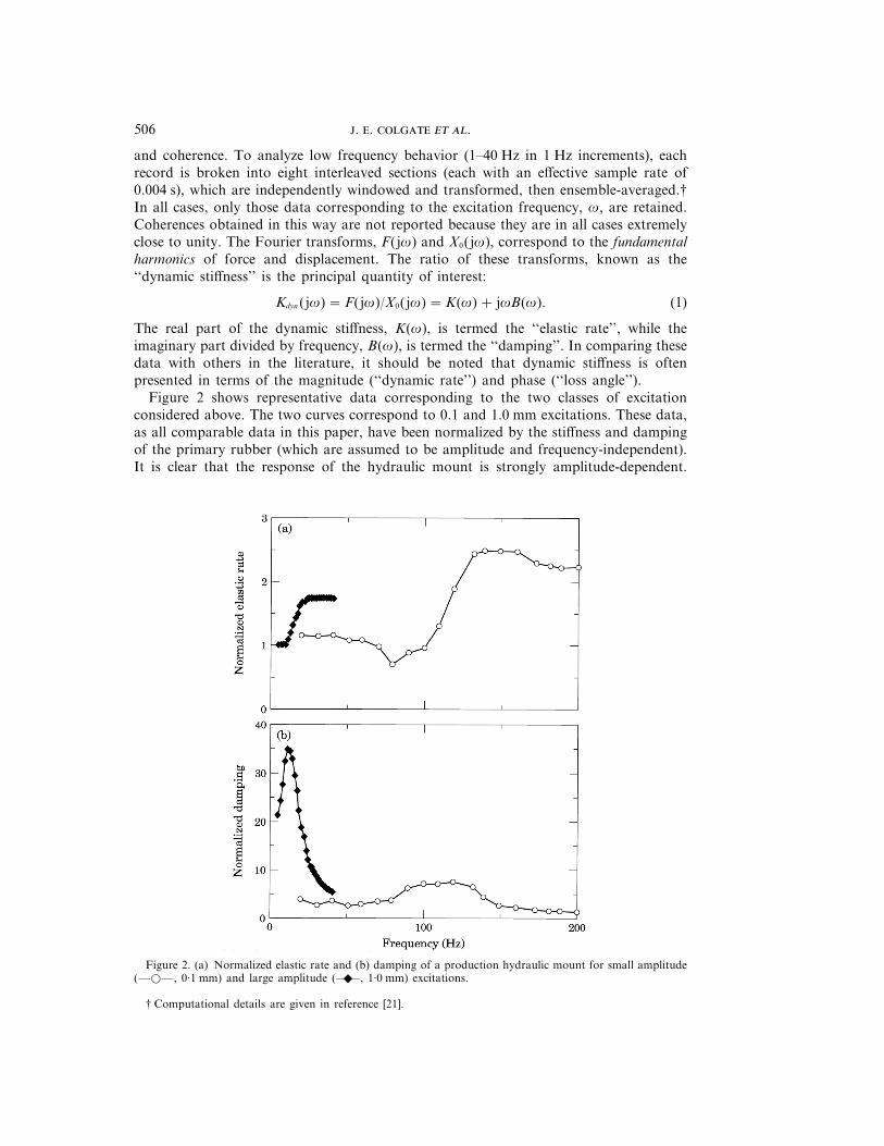
Figure 2 shows representative data corresponding to the two classes of excitationconsidered above. The two curves correspond to 0.1 and 1.0 mm excitations. These data,as all comparable data in this paper, have been normalized by the stiffness and dampingof the primary rubber (which are assumed to be amplitude and frequency-independent).It is clear that the response of the hydraulic mount is strongly amplitude-dependent.

Figure 2. (a) Normalized elastic rate and (b) damping of a production hydraulic mount for small amplitude(—w—, 0·1 mm) and large amplitude (——E , 1·0 mm) excitations.

† Computational details are given in reference [21].

507

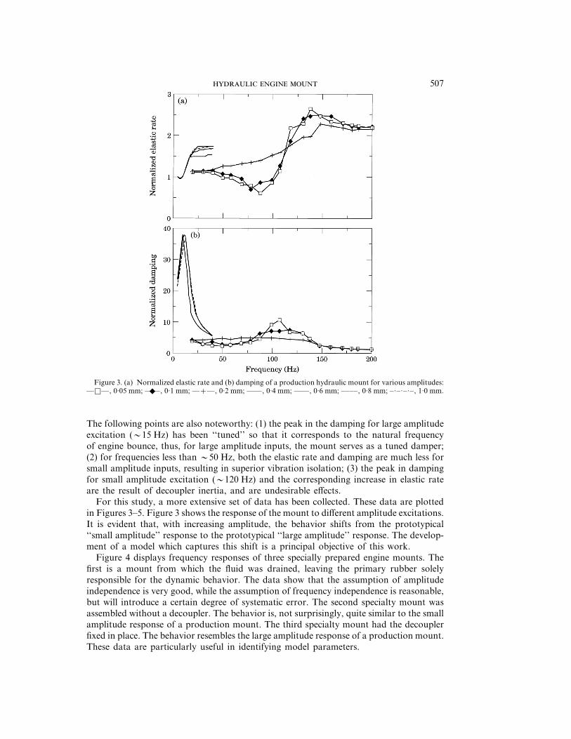
Figure 3. (a) Normalized elastic rate and (b) damping of a production hydraulic mount for various amplitudes:—q—, 0·05 mm; ——E , 0·1 mm; —+—, 0·2 mm; ——, 0·4 mm; ——, 0·6 mm; ––––, 0·8 mm; –·–·–·–, 1·0 mm.

The following points are also noteworthy: (1) the peak in the damping for large amplitudeexcitation (015 Hz) has been ‘‘tuned’’ so that it corresponds to the natural frequencyof engine bounce, thus, for large amplitude inputs, the mount serves as a tuned damper;(2) for frequencies less than 050 Hz, both the elastic rate and damping are much less forsmall amplitude inputs, resulting in superior vibration isolation; (3) the peak in dampingfor small amplitude excitation (0120 Hz) and the corresponding increase in elastic rateare the result of decoupler inertia, and are undesirable effects.

For this study, a more extensive set of data has been collected. These data are plottedin Figures 3–5. Figure 3 shows the response of the mount to different amplitude excitations.It is evident that, with increasing amplitude, the behavior shifts from the prototypical‘‘small amplitude’’ response to the prototypical ‘‘large amplitude’’ response. The develop-ment of a model which captures this shift is a principal objective of this work.

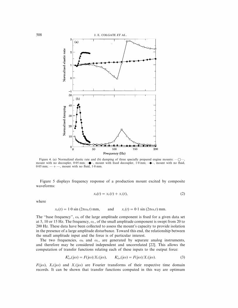
Figure 4 displays frequency responses of three specially prepared engine mounts. Thefirst is a mount from which the fluid was drained, leaving the primary rubber solelyresponsible for the dynamic behavior. The data show that the assumption of amplitudeindependence is very good, while the assumption of frequency independence is reasonable,but will introduce a certain degree of systematic error. The second specialty mount wasassembled without a decoupler. The behavior is, not surprisingly, quite similar to the smallamplitude response of a production mount. The third specialty mount had the decouplerfixed in place. The behavior resembles the large amplitude response of a production mount.These data are particularly useful in identifying model parameters.

. . .508

Figure 4. (a) Normalized elastic rate and (b) damping of three specially prepared engine mounts: —q—,mount with no decoupler, 0·05 mm; ——W , mount with fixed decoupler, 1·0 mm; ——E , mount with no fluid,0·05 mm; —+—, mount with no fluid, 1·0 mm.

Figure 5 displays frequency response of a production mount excited by compositewaveforms:

x0(t)= xb (t)+ xs (t), (2)

where

xb (t)=1·0 sin (2pvbt) mm, and xs (t)=0·1 sin (2pvst) mm.

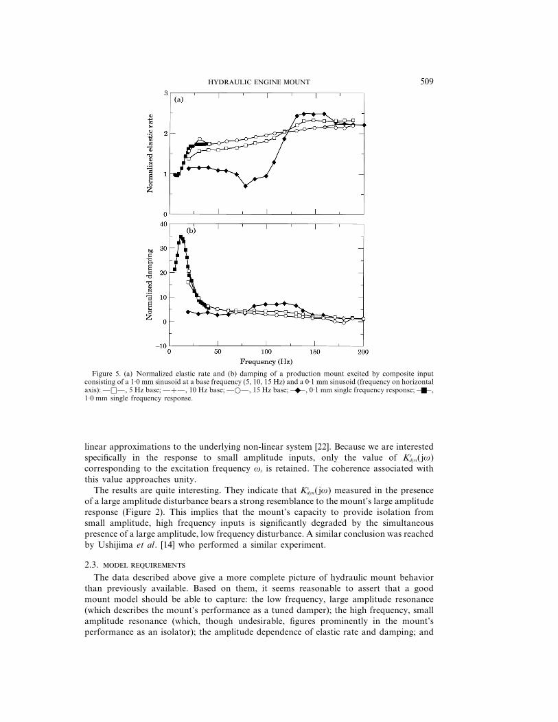
The ‘‘base frequency’’, vb of the large amplitude component is fixed for a given data setat 5, 10 or 15 Hz. The frequency, vs , of the small amplitude component is swept from 20 to200 Hz. These data have been collected to assess the mount’s capacity to provide isolationin the presence of a large amplitude disturbance. Toward this end, the relationship betweenthe small amplitude input and the force is of particular interest.

The two frequencies, vb and vs , are generated by separate analog instruments,and therefore may be considered independent and uncorrelated [22]. This allows thecomputation of transfer functions relating each of these inputs to the output force:

Kbdyn( jv)=F( jv)/Xb ( jv), Ks

dyn( jv)=F( jv)/Xs ( jv). (3)

F( jv), Xb ( jv) and Xs ( jv) are Fourier transforms of their respective time domainrecords. It can be shown that transfer functions computed in this way are optimum

509

Figure 5. (a) Normalized elastic rate and (b) damping of a production mount excited by composite inputconsisting of a 1·0 mm sinusoid at a base frequency (5, 10, 15 Hz) and a 0·1 mm sinusoid (frequency on horizontalaxis): —q—, 5 Hz base; —+—, 10 Hz base; —w—, 15 Hz base; ——E , 0·1 mm single frequency response; ——Q ,1·0 mm single frequency response.

linear approximations to the underlying non-linear system [22]. Because we are interestedspecifically in the response to small amplitude inputs, only the value of Ks

dyn( jv)corresponding to the excitation frequency vs is retained. The coherence associated withthis value approaches unity.

The results are quite interesting. They indicate that Ksdyn( jv) measured in the presence

of a large amplitude disturbance bears a strong resemblance to the mount’s large amplituderesponse (Figure 2). This implies that the mount’s capacity to provide isolation fromsmall amplitude, high frequency inputs is significantly degraded by the simultaneouspresence of a large amplitude, low frequency disturbance. A similar conclusion was reachedby Ushijima et al. [14] who performed a similar experiment.

2.3.

The data described above give a more complete picture of hydraulic mount behaviorthan previously available. Based on them, it seems reasonable to assert that a goodmount model should be able to capture: the low frequency, large amplitude resonance(which describes the mount’s performance as a tuned damper); the high frequency, smallamplitude resonance (which, though undesirable, figures prominently in the mount’sperformance as an isolator); the amplitude dependence of elastic rate and damping; and

. . .510

the mount’s response to composite inputs (which measures the mount’s ability to providesimultaneous isolation and control).

The next section introduces two linear models. These models embody our basic physicalunderstanding of the hydraulic mount, and are sufficient to capture the two resonances.Section 4 presents two approaches to estimating non-linear frequency responses, apiecewise linear simulation and an equivalent linearization analysis. These techniques arealso extended to predict the mount’s response to composite inputs. Section 5 presents asummary discussion.

3. LARGE AND SMALL AMPLITUDE LINEAR MODELS

In this section, two linear models are introduced. The first is tailored to large ampli-tude sinusoidal excitation (q0·5 mm), and makes the assumption that the decoupleris ‘‘bottomed out’’ at all times. The second is tailored to small amplitude excitation(Q0·5 mm), and makes the assumption that the decoupler never bottoms out. Both modelsassume that all other important physical effects may be represented by lumped, lineartime-invariant elements.

3.1.

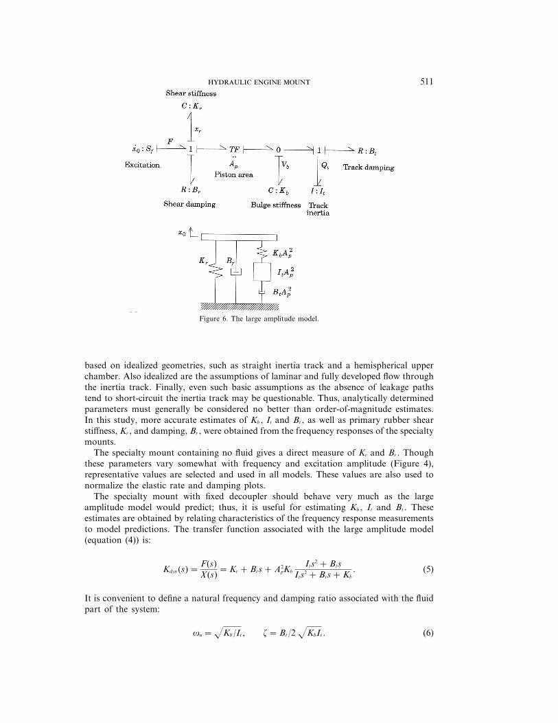
The principal physical effects are taken to be those associated with the primary rubber(shear stiffness and damping; bulge stiffness; piston area) and with the inertia track (fluidinertia and damping). The stiffness of the secondary rubber is small enough that it can beignored (reducing the requisite state dimension by one).† The fluid is assumed incompress-ible (the bulge compliance of the primary rubber is much greater), and the fluid inertiaand damping in the upper chamber are ignored (inertia and damping in the track are muchgreater). The interconnection of these elements is straightforward—both bond graph[23, 24] and mechanical equivalent models are shown in Figure 6. Similar models havebeen presented in references [2, 5, 7, 11, 14].

State equations and an output equation for the reaction force may be derived from thebond graph. They are

& xr

V� b

Q� t'= &000 00

Kb /It

0−1

−Bt /It'&xr

Vb

Qt'+ & 1Ap

0 'x0, (4)

F=[Kr ApKb 0]&xr

Vb

Qt'+[Br ]x0.

The states are shear displacement of the primary rubber (xr ), bulge displacement of theprimary rubber (Vb ) and volumetric flow in the inertia track (Qt ).

Parameter values were obtained as follows. Ap , the ‘‘piston area’’ of the primary rubber,is equal to the area of the orifice plate top surface, which is easily measured. Initialestimates of bulge stiffness, Kb , track inertia, It , and track damping, Bt , were made usingthe analytical formulas given in Singh et al. [11]. These formulas, however, are necessarily

† This may be understood by comparing the response of the mount without fluid to the responses of thefluid-filled mounts. At low frequency, both rubber shear stiffness and secondary rubber stiffness should contributeto the elastic rate of the latter class; yet, these mounts exhibit nearly the same values as the dry mount (Figure4). Measurements of primary rubber bulge compliance and secondary rubber compliance presented by Kim andSingh [20] also indicate that the latter is at least an order of magnitude greater.

511

Figure 6. The large amplitude model.

based on idealized geometries, such as straight inertia track and a hemispherical upperchamber. Also idealized are the assumptions of laminar and fully developed flow throughthe inertia track. Finally, even such basic assumptions as the absence of leakage pathstend to short-circuit the inertia track may be questionable. Thus, analytically determinedparameters must generally be considered no better than order-of-magnitude estimates.In this study, more accurate estimates of Kb , It and Bt , as well as primary rubber shearstiffness, Kr , and damping, Br , were obtained from the frequency responses of the specialtymounts.

The specialty mount containing no fluid gives a direct measure of Kr and Br . Thoughthese parameters vary somewhat with frequency and excitation amplitude (Figure 4),representative values are selected and used in all models. These values are also used tonormalize the elastic rate and damping plots.

The specialty mount with fixed decoupler should behave very much as the largeamplitude model would predict; thus, it is useful for estimating Kb , It and Bt . Theseestimates are obtained by relating characteristics of the frequency response measurementsto model predictions. The transfer function associated with the large amplitude model(equation (4)) is:

Kdyn (s)=F(s)X(s)

=Kr +Brs+A2pKb

Its2 +BtsIts2 +Bts+Kb

. (5)

It is convenient to define a natural frequency and damping ratio associated with the fluidpart of the system:

vn =zKb /It , z=Bt /2 zKbIt . (6)

. . .512

The frequency response may then be written in terms of real (elastic rate) and imaginary(damping) parts:

Kdyn ( jv)=$Kr +A2pKb

v2(v2 −v2n)+4z2v2

nv2

(v2 −v2n)2 +4z2v2

nv2 %

+jv$Br +A2pKb

2zv3n

(v2 −v2n)2 +4z2v2

nv2%, (7)

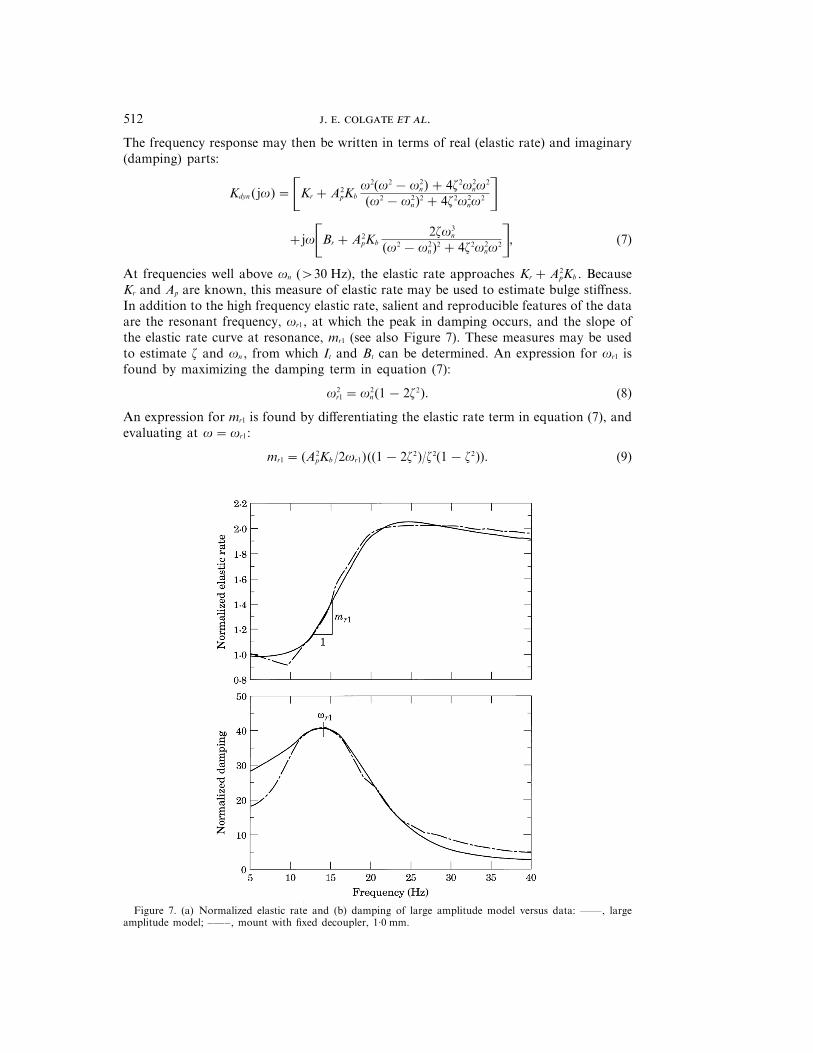
At frequencies well above vn (q30 Hz), the elastic rate approaches Kr +A2pKb . Because

Kr and Ap are known, this measure of elastic rate may be used to estimate bulge stiffness.In addition to the high frequency elastic rate, salient and reproducible features of the dataare the resonant frequency, vr1, at which the peak in damping occurs, and the slope ofthe elastic rate curve at resonance, mr1 (see also Figure 7). These measures may be usedto estimate z and vn , from which It and Bt can be determined. An expression for vr1 isfound by maximizing the damping term in equation (7):

v2r1 =v2

n(1−2z2). (8)

An expression for mr1 is found by differentiating the elastic rate term in equation (7), andevaluating at v=vr1:

mr1 = (A2pKb /2vr1)((1−2z2)/z2(1− z2)). (9)

Figure 7. (a) Normalized elastic rate and (b) damping of large amplitude model versus data: ——, largeamplitude model; –—–, mount with fixed decoupler, 1·0 mm.

513

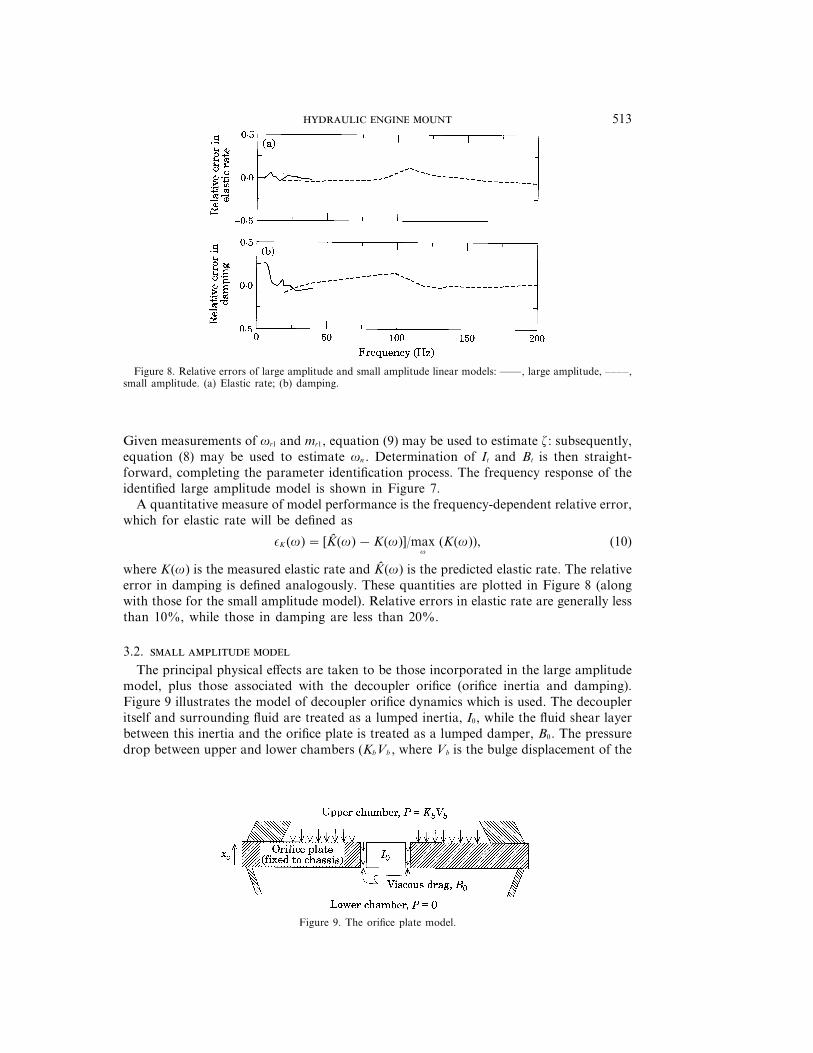
Figure 8. Relative errors of large amplitude and small amplitude linear models: ——, large amplitude, ––––,small amplitude. (a) Elastic rate; (b) damping.

Given measurements of vr1 and mr1, equation (9) may be used to estimate z: subsequently,equation (8) may be used to estimate vn . Determination of It and Bt is then straight-forward, completing the parameter identification process. The frequency response of theidentified large amplitude model is shown in Figure 7.

A quantitative measure of model performance is the frequency-dependent relative error,which for elastic rate will be defined as

eK (v)= [K (v)−K(v)]/maxv

(K(v)), (10)

where K(v) is the measured elastic rate and K (v) is the predicted elastic rate. The relativeerror in damping is defined analogously. These quantities are plotted in Figure 8 (alongwith those for the small amplitude model). Relative errors in elastic rate are generally lessthan 10%, while those in damping are less than 20%.

3.2.

The principal physical effects are taken to be those incorporated in the large amplitudemodel, plus those associated with the decoupler orifice (orifice inertia and damping).Figure 9 illustrates the model of decoupler orifice dynamics which is used. The decoupleritself and surrounding fluid are treated as a lumped inertia, I0, while the fluid shear layerbetween this inertia and the orifice plate is treated as a lumped damper, B0. The pressuredrop between upper and lower chambers (KbVb , where Vb is the bulge displacement of the

Figure 9. The orifice plate model.

. . .514

primary rubber) drives the orifice flow, Q0. A pressure balance gives

KbVb = I0Q� 0 +B0(Q0 −Adxc ). (11)

Ad is the cross-sectional area of the orifice, and xc is the displacement of the chassis, towhich the orifice plate is fixed.

An expression for the force transmitted to the chassis can also be derived with theassistance of Figure 9. Contributions are the forces transmitted via rubber shear, thenormal forces on the orifice plate due to pressure, and the shear forces due to drag:

F=Kr (xe − xc )+Br (xe − xc )+ (Ap −Ad )KbVb +(A2dB0)(Q0/Ad − xc ), (12)

where xe is the displacement of the engine.The effect of orifice dynamics, as represented in equations (11) and (12), can be added

to the large amplitude model by recognizing that the pressure drop across the inertia trackis the same as that across the decoupler orifice. A complete small amplitude model is shownin Figure 10. A mechanical equivalent to this bond graph can be found, but is quitenon-intuitive.

One interesting aspect of the small amplitude model is that it requires two inputs (xe andxc ) rather than a single input (x0 = xe − xc ). The relative displacement is an appropriateinput only in instances when either the engine or the chassis serves as an inertial groundand therefore a proper reference for the orifice inertia.† While no such instance occurs inan automobile, it does occur in the test fixture described in section 2.2 which fixes thechassis bracket to ground (xc =0). In this case, state and output equations are

GG

G

K

k

xr

V� b

Q� t

Q� 0

GG

G

L

l=G

G

G

K

k

0000

00

Kb /It

Kb /I0

0−1

−Bt /It

0

0−1

0−B0/I0

GG

G

L

lGG

G

K

k

xr

Vb

Qt

Q0

GG

G

L

l+G

G

G

K

k

1Ap

00

GG

G

L

lx0, (13)

F=[Kr (Ap −Ad )Kb 0 AdB0]GG

G

K

k

xr

Vb

Qt

Q0

GG

G

L

l+[Br ]x0.

All variables retain previous definitions. The only parameters which did not appear in thelarge amplitude model re Ad , I0 and B0.

The decoupler cross-sectional area is easily measured. Orifice inertia and damping canbe estimated by a procedure similar to that used to find track inertia and damping. Tosimplify the analysis, it is first assumed that, at the frequency of orifice resonance(v2 1 120 Hz), flow through the inertia track can be neglected. This simplification givesthe dynamic stiffness of the small amplitude model a form very similar to equation (5):

Kdyn (s)=F(s)X(s)

=Kr +Brs+A2pKb

(1− e)I0s2 +B0sI0s2 +B0s+Kb

, (14)

where e=Ad /Ap . Equation (14) may be used to develop expressions for the resonantfrequency (vr2) and slope of the elastic rate plot at resonance (mr2). These expressionsmay be equated to values measured using the speciality mount with no decoupler, andsolved to yield estimates of I0 and B0. This process is similar to that used to estimate

† This is not an issue with the track inertia because flow in the track is perpendicular to the assumed axis ofmotion.

515

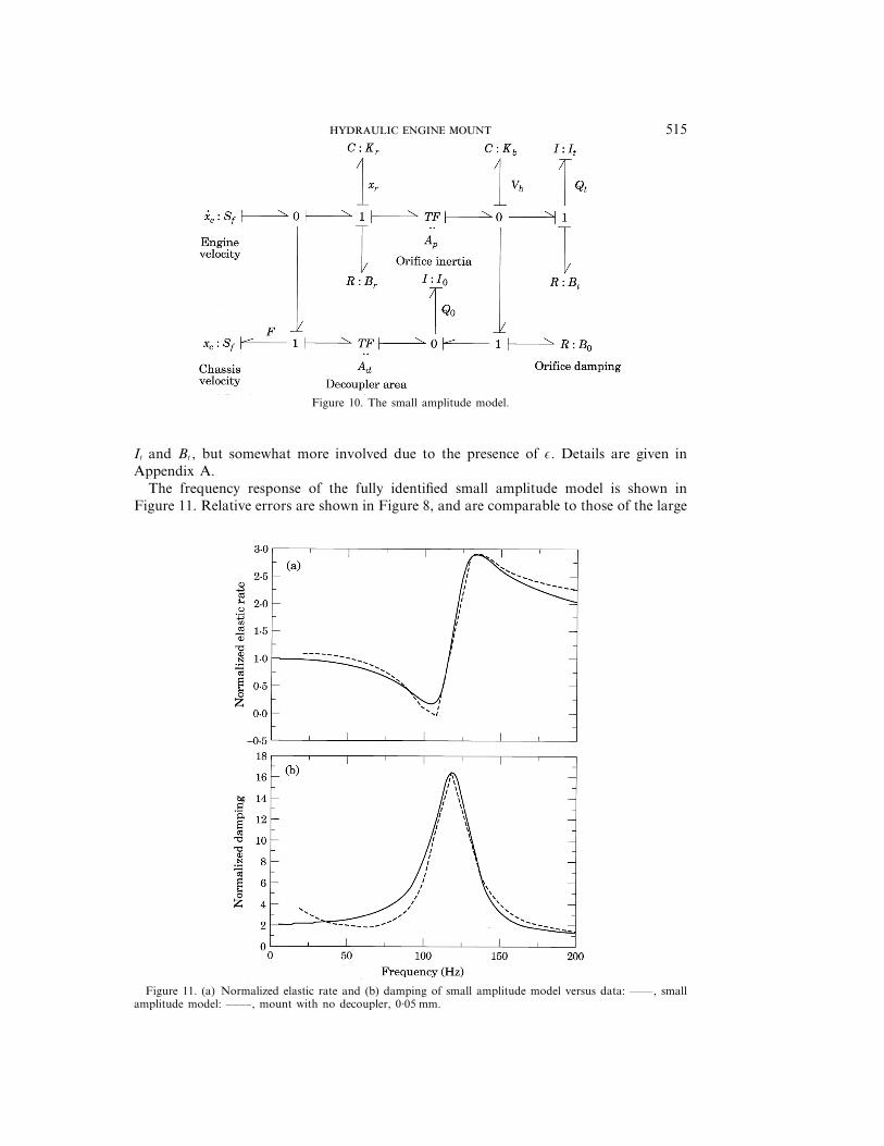
Figure 10. The small amplitude model.

It and Bt , but somewhat more involved due to the presence of e. Details are given inAppendix A.

The frequency response of the fully identified small amplitude model is shown inFigure 11. Relative errors are shown in Figure 8, and are comparable to those of the large

Figure 11. (a) Normalized elastic rate and (b) damping of small amplitude model versus data: ——, smallamplitude model: ––––, mount with no decoupler, 0·05 mm.

. . .516

magnitude model. Although the linear models successfully capture the two resonances,they cannot represent in any greater detail the amplitude dependence of the mount’sresponse. To meet this objective, two non-linear models are introduced.

4. NON-LINEAR MODELLING

A variety of non-linear effects contributes significantly to the behavior of a productionhydraulic mount [20]. These include, for instance, entrance and exit effects in the inertiatrack flow, and amplitude-dependent softening of the primary rubber. In this paper,however, attention will be focused on the decoupler, which is principally responsible forthe amplitude dependence.

4.1.

A direct approach to incorporating decoupler behavior is via a piecewise linear model[19, 25]. In essence, the piecewise linear model reduces to the small amplitude linear model(augmented with a state for decoupler position, xd ) whenever the decoupler is notbottomed out, and to the large amplitude model when the decoupler is bottomed out. Thebehavior of the model can be investigated using numerical integration. The modeldeveloped in reference [25] uses the following scheme for switching during a time domainintegration (d is half the gap width):

If the previous step was integrated with the small amplitude model: if =xd =Q d,integrate small amplitude state equations; if =xd =e d and sign (Vb)= sign (xd ), set Q0 =0,set xd =sign (xd )d, and integrate large amplitude state equations.

If the previous step was integrated with the large amplitude model: if sign (Vb )= sign(xd ), integrate large amplitude state equations; if sign (Vb )$ sign (xd ), integrate smallamplitude state equations.

Note that Vb is linearly related to the pressure in the upper chamber, which determineswhether a decoupler at the limits of its travel will remain bottomed out or not.

A piecewise linear model has several attractive features. No new dynamic elements needbe introduced to account for bottoming out, nor do the (possibly very fast) dynamics ofthe bottoming out process need to be directly considered. Moreover, the linear continuousstate equations can be directly mapped to difference equations which are guaranteed stable[26], so that an efficient simulation can be performed. Finally, excitations of arbitrary shapeare easily accommodated.

A significant disadvantage, however, is that a tremendous amount of time domainsimulation data must be generated to produce a modest amount of frequency domain data.Frequency responses have been computed as follows. A sinusoidal excitation of amplitudeX0 and frequency v is assumed. A simulation time increment of 2p/v/64 seconds is picked,and time domain records of approximately 1150 points are computed. Records includeposition input and force output information. The beginning of each record is cut off toremove the transient response, leaving a record of 1024 points. This record is broken intothree overlapping sections of 512 points each, which are Hanning windowed andtransformed with an FFT. A complex transfer function is computed at the frequency ofexcitation.

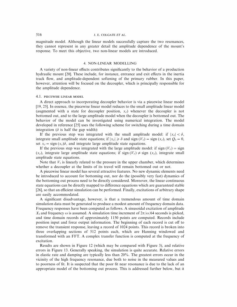
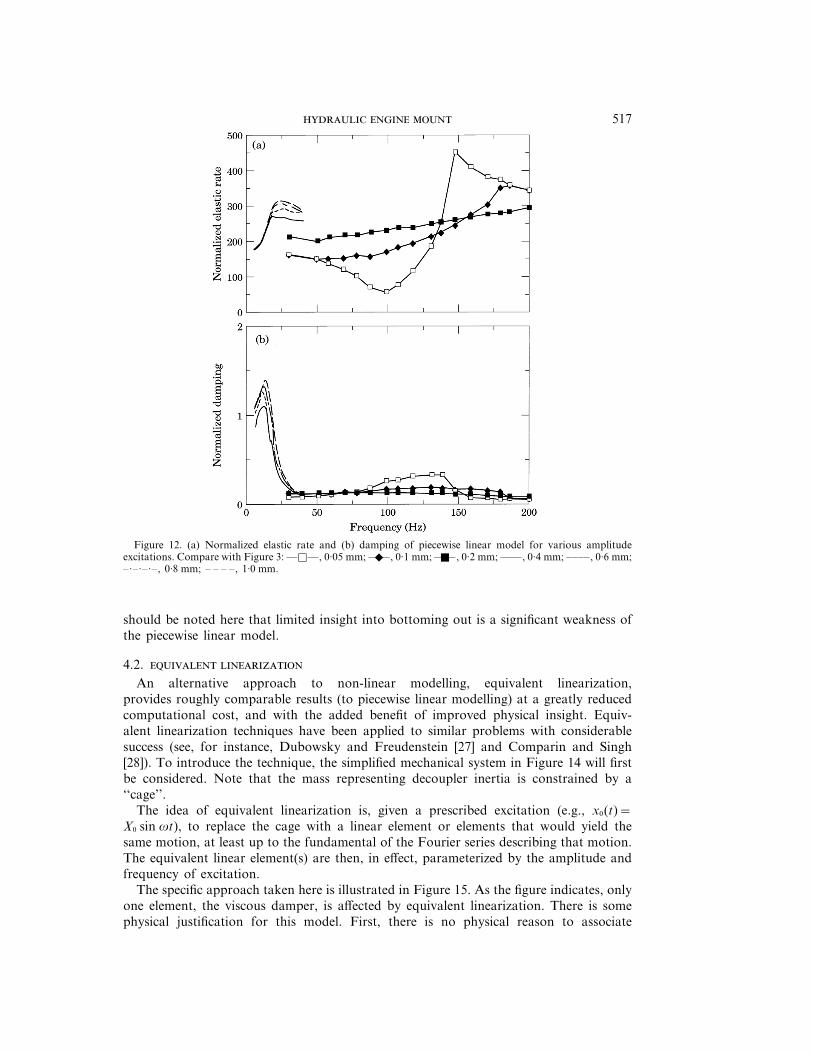
Results are shown in Figure 12 (which may be compared with Figure 3), and relativeerrors in Figure 13. Generally speaking, the simulation is quite accurate. Relative errorsin elastic rate and damping are typically less than 20%. The greatest errors occur in thevicinity of the high frequency resonance, due both to noise in the measured values andto poorness of fit. It is suspected that the poor fit near resonance is due to the lack of anappropriate model of the bottoming out process. This is addressed further below, but it

517

Figure 12. (a) Normalized elastic rate and (b) damping of piecewise linear model for various amplitudeexcitations. Compare with Figure 3: —q—, 0·05 mm; ——E , 0·1 mm; ——Q , 0·2 mm; ——, 0·4 mm; ––––, 0·6 mm;–·–·–·–, 0·8 mm; – – – –, 1·0 mm.

should be noted here that limited insight into bottoming out is a significant weakness ofthe piecewise linear model.

4.2.

An alternative approach to non-linear modelling, equivalent linearization,provides roughly comparable results (to piecewise linear modelling) at a greatly reducedcomputational cost, and with the added benefit of improved physical insight. Equiv-alent linearization techniques have been applied to similar problems with considerablesuccess (see, for instance, Dubowsky and Freudenstein [27] and Comparin and Singh[28]). To introduce the technique, the simplified mechanical system in Figure 14 will firstbe considered. Note that the mass representing decoupler inertia is constrained by a‘‘cage’’.

The idea of equivalent linearization is, given a prescribed excitation (e.g., x0(t)=X0 sin vt), to replace the cage with a linear element or elements that would yield thesame motion, at least up to the fundamental of the Fourier series describing that motion.The equivalent linear element(s) are then, in effect, parameterized by the amplitude andfrequency of excitation.

The specific approach taken here is illustrated in Figure 15. As the figure indicates, onlyone element, the viscous damper, is affected by equivalent linearization. There is somephysical justification for this model. First, there is no physical reason to associate

. . .518

Figure 13. Relative errors for piecewise linear model: —q—, 0·05 mm; ——E , 0·1 mm; ——Q , 0·2 mm; ——,0·4 mm; ----, 0·6 mm; –·–·–·–, 0·8 mm; – – – –, 1·0 mm. (a) Elastic rate; (b) damping.

significant energy storage (potential or kinetic) with bottoming out. Second, the decoupleris immersed in a fluid which must be displaced as the cage boundaries are approached.Thus, a squeeze film [29] is developed. It is well-known that the squeeze film betweenparallel plates produces a damping force which varies as the inverse cube of the gap[29, 30]:

Fsq = g(h� /h3) (15)

Here, h is the gap thickness and g is a geometric parameter. For simple geometries,equation (15) is readily derived from the Reynolds equation for viscous flow [30].The geometry of decoupler/cage interaction is not simple, but it has been assumed thatthe inverse cube form holds nonetheless. The implications of this assumption will bereassessed below. Because the cage in Figure 14 has two sides, the appropriate damping

Figure 14. The simplified model.

519

Figure 15. The model which treats the decoupler cage as an amplitude-dependent dissipator.

relation is

Fsq (xd , xd )= g$ 1(d− xd )3 +

1(d+ xd )3%xd , Fsq (x, x

.)= bd$ 1+3x2

(1+ x2)3%x. , (16a, b)

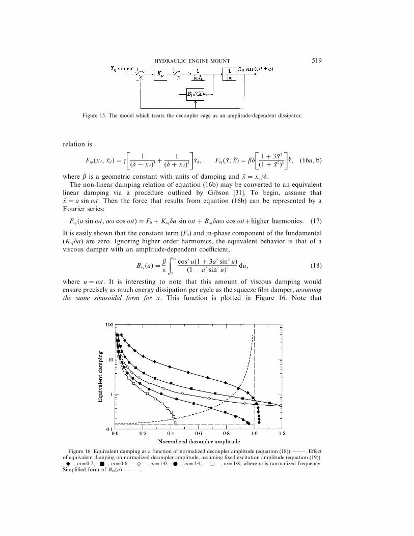
where b is a geometric constant with units of damping and x= xd /d.The non-linear damping relation of equation (16b) may be converted to an equivalent

linear damping via a procedure outlined by Gibson [31]. To begin, assume thatx= a sin vt. Then the force that results from equation (16b) can be represented by aFourier series:

Fsq (a sin vt, av cos vt)=F0 +Keqda sin vt+Beqdav cos vt+higher harmonics. (17)

It is easily shown that the constant term (F0) and in-phase component of the fundamental(Keqda) are zero. Ignoring higher order harmonics, the equivalent behavior is that of aviscous damper with an amplitude-dependent coefficient,

Beq (a)=b

p g2p

0

cos2 u(1+3a2 sin2 u)(1− a2 sin2 u)3 du, (18)

where u=vt. It is interesting to note that this amount of viscous damping wouldensure precisely as much energy dissipation per cycle as the squeeze film damper, assumingthe same sinusoidal form for x. This function is plotted in Figure 16. Note that

Figure 16. Equivalent damping as a function of normalized decoupler amplitude (equation (18)): ––––. Effectof equivalent damping on normalized decoupler amplitude, assuming fixed excitation amplitude (equation (19)):——E , v=0·2; ——Q , v=0·6; —e—, v=1·0; ——W , v=1·4; —q—, v=1·8; where v is normalized frequency.Simplified form of Beq (a) ———.

. . .520

the equivalent damping approaches infinity as the normalized decoupler amplitude, a,approaches 1.

If B0 f(x) in Figure 15 is replaced with Beq , a transfer function may be found relatingX( jv) to X0( jv). The magnitude of this transfer function can be considered an expressionfor the normalized decoupler amplitude in terms of equivalent damping, excitationamplitude and frequency:

a(Beq , X0, v)=Xd

=Kb

z(Kb − I0v2)2 + (Beqv)2

X0

d. (19)

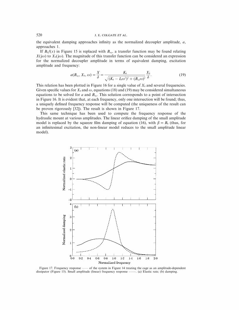
This relation has been plotted in Figure 16 for a single value of X0 and several frequencies.Given specific values for X0 and v, equations (18) and (19) may be considered simultaneousequations to be solved for a and Beq . This solution corresponds to a point of intersectionin Figure 16. It is evident that, at each frequency, only one intersection will be found; thus,a uniquely defined frequency response will be computed (the uniqueness of the result canbe proven rigorously [32]). The result is shown in Figure 17.

This same technique has been used to compute the frequency response of thehydraulic mount at various amplitudes. The linear orifice damping of the small amplitudemodel is replaced by the squeeze film damping of equation (16), with b=B0 (thus, foran infinitesimal excitation, the non-linear model reduces to the small amplitude linearmodel).

Figure 17. Frequency response —— of the system in Figure 14 treating the cage as an amplitude-dependentdissipator (Figure 15). Small amplitude (linear) frequency response ––––. (a) Elastic rate; (b) damping.

521

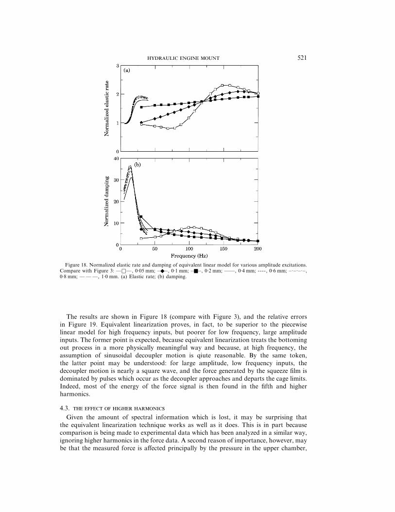
Figure 18. Normalized elastic rate and damping of equivalent linear model for various amplitude excitations.Compare with Figure 3: —q—, 0·05 mm; ——E , 0·1 mm; ——Q , 0·2 mm; ——, 0·4 mm; ----, 0·6 mm; –·–·–·–,0·8 mm; — — —, 1·0 mm. (a) Elastic rate; (b) damping.

The results are shown in Figure 18 (compare with Figure 3), and the relative errorsin Figure 19. Equivalent linearization proves, in fact, to be superior to the piecewiselinear model for high frequency inputs, but poorer for low frequency, large amplitudeinputs. The former point is expected, because equivalent linearization treats the bottomingout process in a more physically meaningful way and because, at high frequency, theassumption of sinusoidal decoupler motion is qiute reasonable. By the same token,the latter point may be understood: for large amplitude, low frequency inputs, thedecoupler motion is nearly a square wave, and the force generated by the squeeze film isdominated by pulses which occur as the decoupler approaches and departs the cage limits.Indeed, most of the energy of the force signal is then found in the fifth and higherharmonics.

4.3.

Given the amount of spectral information which is lost, it may be surprising thatthe equivalent linearization technique works as well as it does. This is in part becausecomparison is being made to experimental data which has been analyzed in a similar way,ignoring higher harmonics in the force data. A second reason of importance, however, maybe that the measured force is affected principally by the pressure in the upper chamber,

. . .522

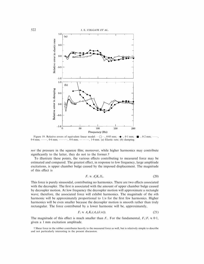
Figure 19. Relative errors of equivalent linear model: —q—, 0·05 mm; ——E , 0·1 mm; ——Q , 0·2 mm; ——,0·4 mm; ––––, 0·6 mm; –·–·–·–, 0·8 mm; — — —, 1·0 mm. (a) Elastic rate; (b) damping.

not the pressure in the squeeze film; moreover, while higher harmonics may contributesignificantly to the latter, they do not to the former.†

To illustrate these points, the various effects contributing to measured force may beestimated and compared. The greatest effect, in response to low frequency, large amplitudeexcitations, is upper chamber bulge caused by the imposed displacement. The magnitudeof this effect is

F1 1A2pKbX0. (20)

This force is purely sinusoidal, contributing no harmonics. There are two effects associatedwith the decoupler. The first is associated with the amount of upper chamber bulge causedby decoupler motion. At low frequency the decoupler motion will approximate a rectanglewave; therefore, the associated force will exhibit harmonics. The magnitude of the nthharmonic will be approximately proportional to 1/n for the first few harmonics. Higherharmonics will be even smaller because the decoupler motion is smooth rather than trulyrectangular. The force contributed by a lower harmonic will be, approximately,

F2 1ApKb (Ad (d/n)). (21)

The magnitude of this effect is much smaller than F1. For the fundamental, F2/F1 1 0·1,given a 1 mm excitation amplitude.

† Shear force in the rubber contributes heavily to the measured force as well, but is relatively simple to describeand not particularly interesting in the present discussion.

523

The second force term is associated with decoupler inertia. This term is simply decouplermass times acceleration, which, for the nth harmonic, is of the order

F3 1 (I0A2d)(d/n)(nv)2 1A2

pKbe2nd(v/vr2)2. (22)

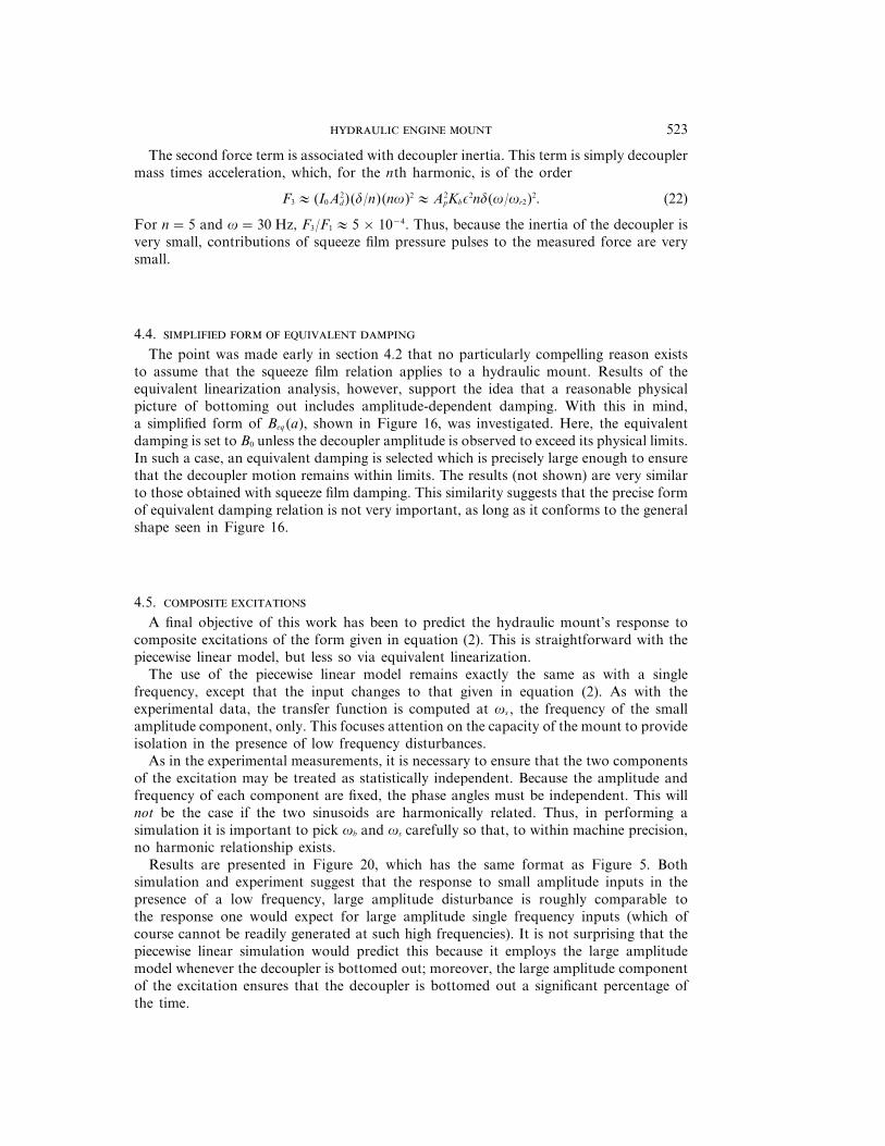
For n=5 and v=30 Hz, F3/F1 1 5×10−4. Thus, because the inertia of the decoupler isvery small, contributions of squeeze film pressure pulses to the measured force are verysmall.

4.4.

The point was made early in section 4.2 that no particularly compelling reason existsto assume that the squeeze film relation applies to a hydraulic mount. Results of theequivalent linearization analysis, however, support the idea that a reasonable physicalpicture of bottoming out includes amplitude-dependent damping. With this in mind,a simplified form of Beq (a), shown in Figure 16, was investigated. Here, the equivalentdamping is set to B0 unless the decoupler amplitude is observed to exceed its physical limits.In such a case, an equivalent damping is selected which is precisely large enough to ensurethat the decoupler motion remains within limits. The results (not shown) are very similarto those obtained with squeeze film damping. This similarity suggests that the precise formof equivalent damping relation is not very important, as long as it conforms to the generalshape seen in Figure 16.

4.5.

A final objective of this work has been to predict the hydraulic mount’s response tocomposite excitations of the form given in equation (2). This is straightforward with thepiecewise linear model, but less so via equivalent linearization.

The use of the piecewise linear model remains exactly the same as with a singlefrequency, except that the input changes to that given in equation (2). As with theexperimental data, the transfer function is computed at vs , the frequency of the smallamplitude component, only. This focuses attention on the capacity of the mount to provideisolation in the presence of low frequency disturbances.

As in the experimental measurements, it is necessary to ensure that the two componentsof the excitation may be treated as statistically independent. Because the amplitude andfrequency of each component are fixed, the phase angles must be independent. This willnot be the case if the two sinusoids are harmonically related. Thus, in performing asimulation it is important to pick vb and vs carefully so that, to within machine precision,no harmonic relationship exists.

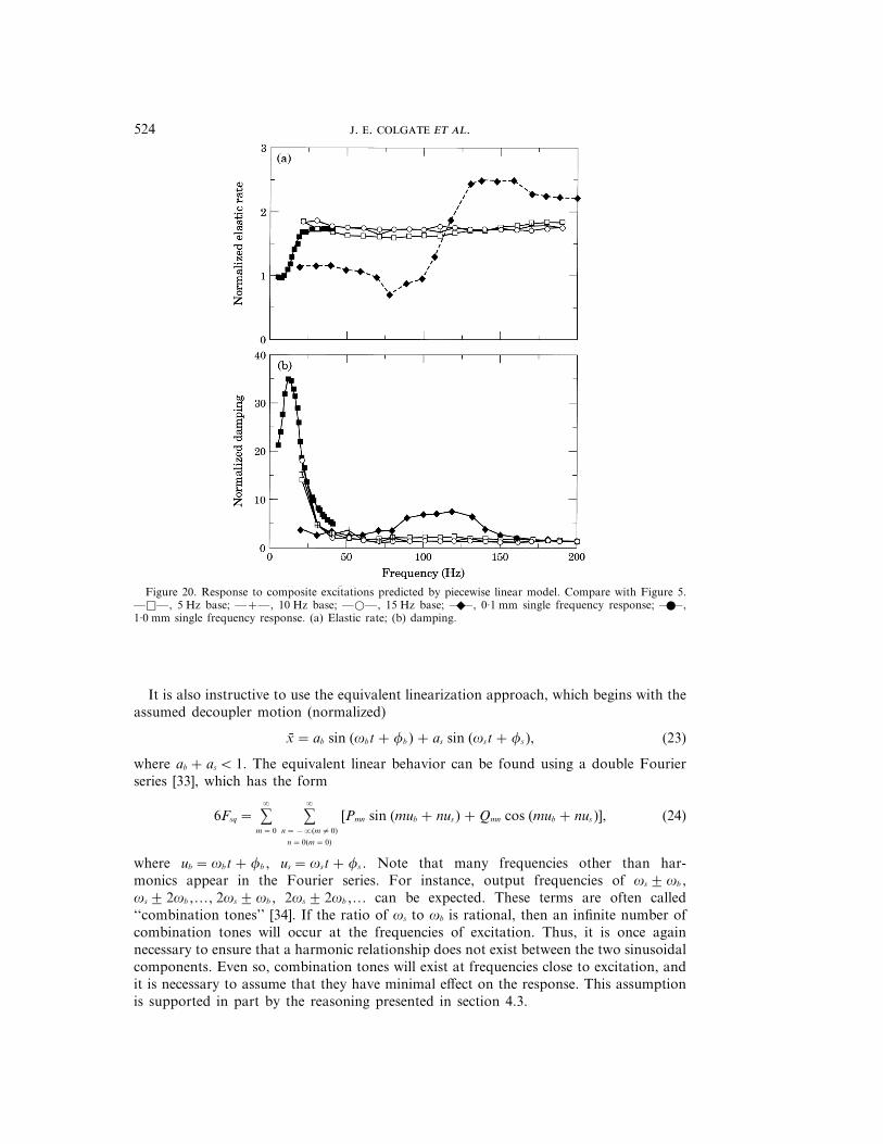
Results are presented in Figure 20, which has the same format as Figure 5. Bothsimulation and experiment suggest that the response to small amplitude inputs in thepresence of a low frequency, large amplitude disturbance is roughly comparable tothe response one would expect for large amplitude single frequency inputs (which ofcourse cannot be readily generated at such high frequencies). It is not surprising that thepiecewise linear simulation would predict this because it employs the large amplitudemodel whenever the decoupler is bottomed out; moreover, the large amplitude componentof the excitation ensures that the decoupler is bottomed out a significant percentage ofthe time.

. . .524

Figure 20. Response to composite excitations predicted by piecewise linear model. Compare with Figure 5.—q—, 5 Hz base; —+—, 10 Hz base; —w—, 15 Hz base; ——E , 0·1 mm single frequency response; ——W ,1·0 mm single frequency response. (a) Elastic rate; (b) damping.

It is also instructive to use the equivalent linearization approach, which begins with theassumed decoupler motion (normalized)

x= ab sin (vbt+fb )+ as sin (vst+fs ), (23)

where ab + as Q 1. The equivalent linear behavior can be found using a double Fourierseries [33], which has the form

6Fsq = sa

m=0

sa

n=−a(m$ 0)

n=0(m=0)

[Pmn sin (mub + nus )+Qmn cos (mub + nus )], (24)

where ub =vbt+fb , us =vst+fs . Note that many frequencies other than har-monics appear in the Fourier series. For instance, output frequencies of vs 2vb ,vs 2 2vb ,..., 2vs 2vb , 2vs 2 2vb ,... can be expected. These terms are often called‘‘combination tones’’ [34]. If the ratio of vs to vb is rational, then an infinite number ofcombination tones will occur at the frequencies of excitation. Thus, it is once againnecessary to ensure that a harmonic relationship does not exist between the two sinusoidalcomponents. Even so, combination tones will exist at frequencies close to excitation, andit is necessary to assume that they have minimal effect on the response. This assumptionis supported in part by the reasoning presented in section 4.3.

525

It is readily shown that Q00, P10 and P01 are all zero, while Q10 and Q01 are non-zero andare related to the equivalent damping at vb and vs , respectively:

Bb (ab , as )=Q10

abvb=

12p2 g

p

−p gp

−p

(cos ub +asvs

abvbcos us )

×1+3(ab sin ub + as sin us )2

(1− (ab sin ub + as sin us )2)3 cos ub dub dus

=1

2p2 gp

−p gp

−p

cos2 ub(1+3(ab sin ub + as sin us )2

(1− (ab sin ub + as sin us )2)3 dub dus , (25)

Bs (ab , as )=Q01

asvs=

12p2 g

p

−p gp

−p 0abvb

asvscos ub +cos us1

×1+3(ab sin ub + as sin us )2

(1− (ab sin ub + as sin us )2)3 cos us dub dus

=1

2p2 gp

−p gp

−p

cos2 us(1+3(ab sin ub + as sin us )2

(1− (ab sin ub + as sin us )2)3 dub dus . (26)

These equations may be used, together with two transfer function relations similar toequation (19) (one at each frequency) to yield a set of four non-linear equations in fourunknowns (Bb , Bs , ab , as ).

A very useful result can be obtained, however, without solving any sets of equations.It is readily shown by direct computation that Bs qBb whenever ab q as . Clearly, wecan expect that the latter condition holds because the excitation amplitude at the basefrequency is ten times larger than that at the higher frequency. Moreover, the equivalentdamping at the base frequency, Bb , must be large enough to limit the decoupler motion. Asseen in the single frequency analysis, this ensures that the frequency response approachesthat of the large amplitude model. The inequality in equivalent damping values thenimplies that the response at the higher frequency, vs , also approaches that of the largeamplitude model. This is in agreement with the behaviors seen in Figures 5 and 20.

5. CONCLUSIONS

Novel experimental data and mathematical models describing a hydraulic engine mounthave been presented. Piecewise linear and equivalent linear models have been shown torepresent hydraulic mount behavior over a broader range of excitations than previouslypossible. While these results provide an excellent basis for hydraulic engine mount analysisand design, they also suggest a number of topics for future research.

For instance, while the large amplitude and small amplitude linear models fit the dataremarkably well, the incorporation of certain additional effects, such as lower chambercompliance, upper chamber bulge damping and leakage past the decoupler, can lead tomoderately improved fits [25]. More importantly, it is possible that some of these effectscould be enhanced to improve the performance of future mount designs. For instance, asignificant increase in upper chamber damping can be used to eliminate the high frequencyresonant peak (with the cost, however, of higher damping at frequencies above resonance).Along similar lines, an interesting adaptive hydraulic mount was recently proposed by Kimand Singh [17]. This concept uses intake manifold vacuum and an electronic controller toswitch the upper chamber compliance between high and low values according to vehicleoperating conditions.

. . .526

Non-linearities other than those associated with the decoupler, such as entrance and exiteffects in the inertia track, may also exert a significant influence on the mount’s behavior[20]. For instance, the over-estimation of damping at frequencies less than 10 Hz (Figure 7)is probably a consequence of having ignored such effects. Thus, future models shouldincorporate other non-linear effects.

The piecewise linear model presented here was particularly adept at capturing lowfrequency amplitude dependence while the equivalent linearization technique was adept athigher frequency. This was because the former did not incorporate a meaningful modelof bottoming out, while the latter was incapable of representing substantially non-sinu-soidal signals. A valuable contribution would be the development of a computationallyefficient model combining the best characteristics of each. This is a challenge becausehigher order equivalent linearization techniques generally require the solution of sets ofnon-linear equations, while a simulation which represents bottoming out explicitly will bestiff.

The two models substantiated experimental results obtained with composite waveforms.The equivalent linearization technique, however, left open the tantalizing possibility thatthe mount’s ability to provide simultaneous control and isolation could be improved withsome other decoupler characteristic. This possibility has also been raised by Ushijima et al.[14], who argue that a rubber membrane decoupler gives better performance than a rigidplate decoupler, as considered here.

Finally, it would be inappropriate to close a discussion of hydraulic engine mountswithout recalling the greater context. Engine mounts are but one contribution to thenoise, vibration and harshness characteristics of an automobile. Hydraulic mounts, inparticular, are designed for significant energetic interaction with the engine and chassis(as an example, the ‘‘apparent inertia’’ of the inertia track, A2

pIt , is comparable to the enginemass). It is reasonable to expect, therefore, that the performance of a hydraulic mountwill be sensitive to the dynamic characteristics of the vehicle in which it isplaced. Moreover, performance must ultimately be considered a matter of subjective(passenger) impression. These factors have to date, and will for the foreseeable future,necessitate a rather lengthy cycle of design, testing and redesign. Thus, it is not simply thehydraulic mount itself, but its role in this broader context which must be the subject offuture studies.

ACKNOWLEDGMENTS

The authors would like to thank Jim Frye, Tony Villanueva and Bill Resh of ChryslerCorporation for their support of this research. The authors would also like to thankEd Probst and his staff at Delco Products for their assistance in supplying and testinghydraulic engine mounts.

REFERENCES

1. W. R 1994 Chrysler Corporation. Personal communication.2. M. B 1984 SAE Paper 840259. A new generation of engine mounts.3. S. B, R. S, T. K and P. S 1989 SAE Paper 891160. Optimal

tuning of adaptive hydraulic engine mounts.4. R. M. B and A. G. H 1993 SAE Paper 931321. On the dynamic response of

hydraulic engine mounts.5. M. C 1985 SAE Paper 851650. Hydraulic engine mount isolation.6. P. E. C and G.-H. T 1984 SAE Paper 840407. Hydraulic engine mount character-

istics.

527

7. W. C. F 1985 SAE Paper 850975. Understanding hydraulic mounts for improved vehiclenoise, vibration and ride qualities.

8. K. K 1989 SAE Paper 891138. Hydraulic engine mount for shock isolation atacceleration on the FWD cars.

9. R. A. M 1984 SAE Paper 840410. Hydraulic mounts—improved engine isolation.10. R. S, P. L. G and T. L. H 1986 SAE Paper 860549. Adaptive hydraulic

engine mounts.11. R. S, G. K and P. V. R 1992 Journal of Sound and Vibration 158, 219–243. Linear

analysis of automotive hydro-mechanical mount with emphasis on decoupler characteristics.12. M. S and E. A 1986 SAE Paper 861412. Optimum application for hydroelastic engine

mount.13. T. U and T. D 1986 SAE Paper 860550. Nonlinear B.B.A. for predicting vibration

of vehicle with hydraulic engine mount.14. T. U, K. T and H. K 1988 SAE Paper 880073. High performance hydraulic

mount for improving vehicle noise and vibration.15. J. P. W 1987 Automotive Engineer 12, 17–19. Hydraulically-damped engine mounts.16. P. L. G, D. N, R. S, J. S and R. W. S 1988 SAE Paper

880074. Active frame vibration control for automotive vehicles with hydraulic engine mount.17. G. K and R. S 1993 in Advanced Automotive Technologies (M. Ahmadian, editor).

247–255. New York: ASME. A broadband adaptive hydraulic mount system.18. R. S, P. L. G, S. B, T. K and R. W. S 1988 SAE Paper

880075. Open-loop versus closed-loop control for hydraulic engine mounts.19. G. K and R. S 1992 in Transportation Systems—1992, 165–180. New York, ASME.

Resonance, isolation and shock control characteristics of automotive nonlinear hydraulic enginemounts.

20. G. K and R. S 1993 Journal of Dynamic Systems, Measurement and Control 115, 482–487.Nonlinear analysis of automotive hydraulic engine mount.

21. C. T. C 1992 Master’s Thesis, Northwestern University. Dynamic analysis of hydraulicengine mounts.

22. J. S. B and A. G. P 1986 Random Data: Analysis and Measurement Procedures.New York: John Wiley.

23. D. K and R. R 1975 System Dynamics: A Unified Approach. New York: JohnWiley.

24. H. M. P 1961 Analysis and Design of Engineering Systems. Cambridge, Massachusetts:MIT Press.

25. Y. C. C 1993 Master’s Thesis, Northwestern University. Computer simulation of hydro-elastic engine mounts.

26. G. F. F, J. D. P and M. L. W 1990 Digital Control of Dynamic Systems.Reading, Massachusetts: Addison-Wesley.

27. S. Dubowsky and F. Freudenstein 1971 Transactions of the American Society of MechanicalEngineers, Journal of Engineering for Industry 93, 310–316. Dynamic analysis of mechanicalsystems with clearances, Part 2: dynamic response.

28. R. J. C and R. S 1989 Journal of Sound and Vibration 134, 259–290. Non-linearfrequency response characteristics of an impact pair.

29. D. F. H 1963 Journal of Basic Engineering 85, 243–246. Squeeze films for rectangular plates.30. W. S. G, H. H. R and S. Y 1966 Journal of Basic Engineering 88,

451–456. A study of fluid squeeze-film damping.31. J. E. G 1963 Nonlinear Automatic Control. New York: McGraw-Hill.32. P.-T. D. S and W. D. I 1978 International Journal of Non-linear Mechanics 13, 71–78.

On the existence and uniqueness of solutions generated by equivalent linearization.33. A. G and W. V-V 1968 Multiple-input Describing Functions and Nonlinear Systems

Design. New York: McGraw-Hill.34. A. U and L. O. C 1984 IEEE Transactions on Circuits and Systems CAS-31(9),

766–778. Frequency-domain analysis of nonlinear circuits driven by multi-tone signals.

APPENDIX A: ORIFICE PROPERTIES

A method of estimating orifice inertia, I0, and damping, B0, based on resonantfrequency, vr2, and slope of the elastic rate plot at resonance, mr2, is presented. The starting

. . .528

point is equation (14), which provides an approximate expression for dynamic stiffness.It is convenient to define a natural frequency and damping ratio as

vn =zKb /I0, z=B0/2zKbI0. (A1)

The frequency response may then be written in terms of real (elastic rate) and imaginary(damping) parts,

Kdyn ( jv)=$Kr +A2pKb

av4 + (4z2 − a)v2nv

2

(v2 −v2n)2 +4z2v2

nv2%

+jv$Br +A2pKb2zvn

2zv2n −(1− a)v2

(v2 −v2n)2 +4z2v2

nv2%, (A2)

where a=1−Ad /Ap . An expression for vr2 is found by maximizing the damping term inequation (A2) with respect to frequency:

v2r2 =v2

n [1−z4(1− a)z2 + a2]/(1− a). (A3)

It is now helpful to define b as

b=[1−z4(1− a)z2 + a2]/(1− a). (A4)

An expression for mr2 is found by differentiating the elastic rate term in equation (A2) withrespect to frequency, and evaluating at v=vr1:

mr2 =2A2

pKb

vr2

×$(2ab2 + b(4z2 − a))((1− b)2 +4z2b)−2(b2 − b(2z2 −1))(ab2 + b(4z2 − a))((1− b)2 +4z2b)2 %.

(A5)

Equation (A5) may be solved for z using a Newton–Raphson technique; subsequently,equation (A3) may be solved for vn . Determination of I0 and B0 is then straightforwardusing equations (A1).