UPTEC W05 039

Examensarbete 20 pAugusti 2005

Modelling Nitrogen Flows in Peri-urban Vegetable Field Plots in Nanjing, China

Josefin Berg

ii

ABSTRACT Modelling Nitrogen Flows in Peri-urban Vegetable Field Plots in Nanjing, China Many parts of China are going through a rapid development and urbanization resulting in various environmental impairities. The Yangtze Delta Region surface water bodies are affected by eutrophication, partly caused by diffuse losses from agriculture. In this study, nitrogen, and to some extent also phosphorus, flows and losses from two plots in an intensively cultivated vegetable field in a peri-urban area of Nanjing, with a high input of organic fertilizer, were analysed by the use of the field-scale simulation model GLEAMS. The GLEAMS model was parameterized and calibrated against measurements of soil water and nitrogen content in two plots. A scenario with a reduced input of nitrogen was then simulated.

The resemblance between simulated and measured water content in the different soil

layers was quite poor. The simulated inorganic nitrogen content in the soil was significantly lower than the measured during great parts of the simulation period. This could be due to an inappropriate simulation of the mineralization of organic N under these conditions, or an underestimated decomposition rate of manure. It is also possible that the poor water simulations contributed to the underestimated inorganic N content in the soil. There were similar results for the two plots, except for an unexplained 20% increase in leaching and erosion losses of N in Plot B. For simulation of scenarios to find best management practices, the model parameterization should be further refined. Keywords: nitrogen, peri-urban agriculture, GLEAMS model, Yangtze Delta, Nanjing, China, manure

iii

REFERAT Modellering av kväveflöden i tätortsnära grönsaksodlingar i Nanjing, Kina Den snabba utvecklingen och urbaniseringen i stora delar av Kina har ett flertal konsekvenser för miljön. Yangtzedeltats ytvatten är till stor del eutrofierade, delvis p.g.a. diffusa förluster från jordbruket. I denna studie har kväve- och, till viss del, fosforflöden och förluster från två odlingsrutor i ett intensivt odlat grönsaksfält i ett tätortsnära område i Nanjing, med hög tillförsel av organiskt gödsel, undersökts med hjälp av den fältskaliga simuleringsmodellen GLEAMS. GLEAMS parametriserades och kalibrerades mot mätvärden av jordens vatten- och kväveinnehåll. Ett scenario med minskad kvävetillförsel simulerades sedan. Simuleringen av vattenhalten i de olika horisonterna var inte utmärkt. Den simulerade mängden mineralkväve i marken var avsevärt lägre än den uppmätta. Detta kan bero på en felaktig simulering av mineraliseringen av organiskt kväve eller en för långsam nedbrytning av gödsel. Det är också möjligt att felen i vattensimuleringarna bidrog till underskattningen av mängden mineralkväve i marken. Simuleringarna på de båda odlingsrutorna gav liknande resultat, förutom att ruta B hade 20% större förluster av N via simulerad erosion och läckage. För fortsatt simulering av alternativa odlingsmetoder bör modellens parametrisering förbättras, särskilt vad avser parametrar kopplade till gödselns mineralisering. Nyckelord: kväve, tätortsnära jordbruk, GLEAMS, Yangtze Delta, Nanjing, Kina, stallgödsel The Swedish University of Agricultural Sciences, Department of Soil Sciences. Box 7014, SE-75007 Uppsala ISSN 1401-5765

iv

PREFACE This final thesis is a part of an MSc degree in Environmental and Aquatic Engineering at Uppsala University and covers 20 Swedish academic credits. The study was initiated by the Department of Soil Sciences at the Swedish University of Agricultural Sciences (SLU) as part of the project RURBIFARM, sponsored by the European Union (Contract no. ICA4-CT-2002-10021). Supervisor has been Dr Martin Larsson at SLU, Department of Soil Sciences. The thesis has been reviewed by Prof Lars Bergström at SLU, Department of Soil Sciences.

This project would not have been possible without the constant support of Dr Martin Larsson. Thank you for the effort you have put into making the model work, for answering my innumerous questions and for the feedback on the report. I wish the best for the continued simulations. Further on I would like to thank the professors and staff , especially Prof Shi Xuezheng, Dr Huang Biao and MSc Yü Dongsheng at the Institute of Soil Science, the Chinese Academy of Sciences in Nanjing for the information provided about the site, and for taking such good care of me during my earlier Minor Field Study in Nanjing. Having been at the site really helps the modelling. Further thanks go to MSc Wang Hongjie for providing me with all the soil data needed for the parameterization and calibration. I also wish the best for MSc candidate Chang Qing and her simulations in Wuxi. Prof Ingrid Öborn and Dr Minha Fagerström at SLU should be mentioned as well for giving me the chance to carry out my master thesis work within the RURBIFARM project. Final thanks go to those who have hosted and supported me during this period: Nicolas in Milano/Antibes, my parents in Stockholm, Johan and Johanna in Uppsala, Marek in Košice, and all my other friends in Europe. I am also grateful for the file area for students at Uppsala University, which kept my work safe when my computer crashed.

Copyright© Josefin Berg and Department of Soil Sciences, Swedish University of Agricultural Sciences UPTEC W 05 039 ISSN 1401-5765 Printed at the Department of Earth Sciences, Geotryckeriet, Uppsala University, Uppsala, 2005.

v

Definitions and Abbreviations A Soil loss in the Universal Soil Loss Equation AMON The ammonium pool in GLEAMS AWMN Mineralization from manure AWRC Composition factor for manure C1 Nitrogen content coefficient CFACT Cover management factor CMN Specific mineralization rate constant CN Curve number CNP Carbon:nitrogen:phosphorous factor Cs Concentration of adsorbed labile P DNI Denitrification E Estimated value EF Efficiency factor FC Field capacity (water content at -33 kPa) K Soil erodibility L Slope length MN Mineralization from POTMIN NFACT Roughness factor (manning’s n) NIT Nitrification O Observed value ORGNW Organic N in manure PFACT Land supporting practice factor PLAB Labile P pool in GLEAMS POR Porosity POTMIN Potentially mineralizable N in GLEAMS PY Potential yield Q SCS runoff R Erodibility factor RNP Ratio of N to P s Retention parameter S Slope steepness SM, SW Water content SORGP Soil organic P in GLEAMS SWFA Soil water factor for ammonification SWFN Soil water factor for nitrification TFA Temperature factor for ammonification TFN Temperature factor for nitrification TN Total N initially in soil TKN Total N TP Total P U Daily rainfall UL Upper limit of water storage WP Wilting point

vi

TABLE OF CONTENTS 1. Introduction………………………………………………………………1 2. Background………………………………………………………………2 2.1. Peri-urban farming and pollution in the Yangtze Delta Region…….2 2.2. Transformation and losses of N and P……………………………....3 2.2.1. Nitrogen transformation and losses…………………………3 2.2.2. Phosphorus transformations and losses……………………..4 2.3. Quantification of nutrient losses…………………………………….4 3. Materials and methods…………………………………………………...5 3.1. Model description…………………………………………………...5 3.1.1. Model overview……………………………………………..5 3.1.2. Hydrological component of the model……………………...6 3.1.3. Erosion component………………………………………….8 3.1.4. Nutrient component…………………………………………8 3.2. Experimental data and measurements……………………………..12 3.2.1. Site description…………………………………………….12 3.2.2. Climate data………………………………………………..12 3.2.3. Soil texture and hydraulic properties………………………12 3.2.4. Measurements of water content and N and P in soil………12 3.2.5. Crop management data and harvest………………………..13 3.3. Model application………………………………………………….14 3.3.1. Parameterization and calibration…………………………..14 3.3.2. Scenario for Plot A………………………………………...16 3.3.3. Investigation of CN………………………………………..17 3.3.4. Model evaluation………………………………………….17 4. Results and discussion…………………………………………………18 4.1. Soil water content…………………………………………………18 4.2. Nutrient uptake……………………………………………………19 4.3. Nitrogen in the soil………………………………………………..22 4.3.1. Total Nitrogen…………………………………………….22 4.3.2. Nitrate and ammonia……………………………………...22 4.4. Phosphorus………………………………………………………..28 4.4.1. Total P…………………………………………………….28 4.5. Sensitivity analysis of CN………………………………………...28 4.6. Comparison of N losses from different management practices…..29

4.7. Summary of the discussion and suggestions for the use of the GLEAMS model………………………………………………….30

5. Conclusions…………………………………………………………….31 6. References……………………………………………………………...32

Appendix A: Parameters used in GLEAMS simulation for Plot A and B……..36 Appendix B: Soil measurements provided by ISSAS………………………….39 Appendix C: Long term N and P simulations of Plot A and Scenario…………40 Appendix D: The effect of wilting point on decomposition of manure………..41

1

1. INTRODUCTION Sustainable agriculture and security of food supply is a challenge in many heavily urbanized regions in Asia, as farmland is giving way for urban settlements. In China, 50% of the population currently live in urban areas as compared to 18% in 1975 (UNDP, 2004a). This increase of population density increases the pollution of air and water. The urban population has a high demand for fresh vegetables (Veeck and Veeck, 2000) of which a significant part currently is met by so called peri-urban agriculture in the vicinity of cities. In China, 85% of the vegetable consumption in the 14 largest cities is produced in the peri-urban areas (UN-Habitat, 2001). The peri-urban agriculture is intensive to meet the high demand, and an inappropriately high input of fertilizers as well as pesticides is common (Huang et al., 2005), thus contributing to the pollution of waters and degradation of soil (Cao et al., 2004). Peri-urban agriculture is also insecure due to the competition of land and labour from the city (Midmore and Jansen, 2003), leading to a management aimed at high profit with little consideration of negative long-term effects. However, peri-urban agriculture can contribute to minimizing nutrient pollution through the recycling of urban wastes, although also this is not without problems (Wang and Tao, 1998; Midmore and Jansen, 2003).

To minimize the pollution from agriculture, nutrient management can become more adapted to the needs of the specific site (Jin and Jiang, 2002). One way of achieving this is through computer simulation models (Richter and Roelcke, 2000). With modelling, nutrient transformations and flows can be analysed without interfering with the actual system being studied. This allows for testing of alternative scenarios in order to find the best management practice (BMP) for a farming system (Djodjic et al., 2002). Modelling can in this way be part of a decision support system for improved management (Schaffer, 1995).

RURBIFARM – ‘Sustainable Farming at the Rural-Urban Interface – An integrated knowledge based approach for the nutrient and water recycling in small-scale farming systems in peri-urban areas of China and Vietnam’ – is a project aiming to contribute to a sustainable development of peri-urban agriculture (RURBIFARM, 2002). The project, running from 2002 to 2006, is a joint project between universities and research institutes in Sweden, the UK, China, Vietnam, and Thailand, as well as the International Centre for Research in Agroforestry (ICRAF) in Indonesia. Responsible for the project in China is the Institute of Soil Science, the Chinese Academy of Sciences (ISSAS). One sub-project in RURBIFARM focuses on quantification of nutrient balances in current agricultural systems at sites in China and Vietnam, with the goal to find alternative management practices that can decrease the pollution of waters from peri-urban agriculture. For this purpose, the simulation model GLEAMS, Groundwater Loading Effects of Agricultural Management Systems (Knisel and Davis, 1999) was chosen. This model has been widely used in Europe and North America for evaluation of the effects from agriculture on water quality, but few reports of its usage in Asian peri-urban agriculture have been found.

The purpose of this study was to apply the GLEAMS model to a peri-urban agricultural site with intensive vegetable based production in Nanjing, China. Nutrient flows and losses are quantified, site-specific input parameters are estimated and the model is evaluated regarding strengths and weaknesses for this specific application.

2

2. BACKGROUND

2.1. PERI-URBAN FARMING AND POLLUTION IN THE YANGTZE DELTA REGION

China has the largest population in the world with 1.3 billion inhabitants, and the population continues growing with 0.6% per year (UNDP, 2004b). In the past 40 years, China has increased its food production, despite a decrease of arable land. This has been possible due to a massive use of mineral fertilizer, mainly N and P. China now uses 30% of the world’s N-fertilizer (Zhu and Chen, 2002), and the usage is expected to have doubled by the year 2020 (Galloway, 2000). This has resulted in a surplus of N and P, which subsequently can result in elevated losses to water and air. There are estimates that up to half of the applied nitrogen in China is lost as volatilization, and up to ten percent is lost to ground and surface waters (Nehru et al., 1997; Norse et al., 2001). These losses have a range of serious environmental consequences, one being that surface waters become eutrophied, which may result in oxygen depletion of waters and harmful algal blooms along the coast, so called red tides (Galloway, 2000). Emissions of N2O contribute to global warning and harm the ozone layer, while NO3 pollution rends groundwater dangerous to health (Brady and Weil, 2002). These environmental problems are present in China today and are not likely to improve within a near future (Galloway, 2000).

Figure 1 Location of the Yangtze Delta Region.

One of the regions severely affected by eutrophication is the heavily urbanized Yangtze Delta Region (YRD), including Shanghai and the provinces of Jiangsu, Zheijang and the eastern part of Anhui (Fig. 1). In this region, occupying 1% of China’s surface, 6% of the population is living and 16% of the country’s GDP is produced (Huang et al., 2005). There is clear evidence of N and P pollution in the area. The Yangtze River transports 774 900 tons of dissolved inorganic nitrogen (DIN) to the East China Sea every year. This annual transport of DIN increased four-fold from 1971 to 2000 (Duan et al., 2000). The Yangtze River now transports about 2% of the world’s river water, and carries about 7% of the world’s river DIN (Duan et al., 2000). Before, red tides were rare in the East China Sea and along the Chinese coastal waters, but they have been increasing since the 1960’s, and since 1989, 12 to 38 harmful algal blooms have been reported every year. There is also considerable concern about the increasing NO3 concentrations of wells in the YRD (Cao et al., 2004). Another example is the eutrophication of Lake Taihu, in the eastern part of the YRD, which greatly affects the region’s social and economic development (Guo et al., 2004). Fifty per cent of the

3

nutrient load in form of N and P to Lake Taihu come from non-point sources, of which Guo et al. (2004) estimated that 48% of the total nitrogen (TN) and 38% of the total phosphorus (TP) come from agricultural land (other sources being village residents, town centre and a poultry factory). As more focus is spent on treating point sources, like urban and industrial wastewater, the non-point sources will increase their relative influence as sources for the discharge of N and P.

Due to the high urbanization of the YRD, the main part of its agriculture is peri-

urban. The peri-urban farmers often grow vegetables instead of the traditional paddy rice-wheat rotation, in order to profit from the high vegetable demand in the cities. This intense production, with up to 5 harvests per year, demands more nutrient input than the paddy rice-wheat system. The increased use of mineral fertilizer has resulted in increased pollution and soil degradation in the region (Cao et al., 2004). As the shallow roots of many vegetables cannot take up nutrients percolating down in the soil, vegetable production can also result in high leaching. Soil degradation from a high use of mineral fertilizer is manifested by acidification, salt accumulation, and an over accumulation of NO3 and available P (Cao et al., 2004). Cao et al. (2004) found that more than 60% of investigated soil samples from the YRD had NO3 contents higher than 200 mg kg-1, which is the limit for when vegetable growth can become damaged.

Generally, the use of manure, from cows, pigs, poultry or humans, has decreased in China, but remains high where available. Gerber et al. (2002) showed that there is an overload of organic nutrients in fields close to animal farms. These farms are often located in peri-urban regions. Wang (2003) puts forward that the intensified animal industry has created ‘gross excesses of certain nutrients being land applied’.

2.2. TRANSFORMATION AND LOSSES OF N AND P 2.2.1. Nitrogen transformation and losses Nitrogen exists in inorganic form as NO3

- and NH4+ in the soil and in organic forms as

e.g. amine groups in organic material. About 95% of the N in soil is normally organic. Inorganic N is available for plant uptake, but also for losses to water and air. Organic N is more stable, although there is soluble organic N which has been shown to leach into groundwater in areas with a high application of manure. Organic N transforms into inorganic N through mineralization, which is a result of hydrolysis of amine groups by soil microbes into NH4. Ammonium can then be oxidized into NO3 through nitrification. Microbes simultaneously take up inorganic N and transform it to organic N through immobilization. A resulting net mineralization or immobilization depends on the ratio of carbon to nitrogen in the nitrogen pools. Nitrogen can also be fixated to the soil from the air by plants and microbes, or it can be lost to the air through denitrification of NO3 to gaseous forms. Ammonium is also lost to the air, but through volatization to NH3 gas, which makes the soil more acidic. Ammonium can also attach to clay minerals and be carried away with erosion, while NO3 is dissolved in water and leached to the groundwater and surface water or washed away with surface runoff. As discussed earlier, these losses may harm the environment, but can be decreased with improved management (Brady and Weil, 2002).

4

2.2.2. Phosphorus transformations and losses One big difference between N and P is that a large part of the P exists in mineral forms, which adsorbs strongly to the soil minerals, while N mainly exists in organic material. Despite of this strong adsorption, some P is lost as leaching of dissolved PO4

2-, and some through surface runoff and erosion of phosphorus-carrying particles. When reaching water bodies, the P bound to particles can become bio-available through desorption processes and cause eutrophication. Since P is adsorbed to the soil, there may be a significant accumulation in the soil if a surplus is applied. This accumulated P is usually in forms not available to plants (Brady and Weil, 2002).

2.3. QUANTIFICATION OF NUTRIENT LOSSES Simulation models are useful tools for quantification of N and P flows and for evaluation of the effects alternative management practices have on the losses (Knisel and Turtola, 2000). Modelling, if properly done, can be cost and time effective compared to field experiments. Once a BMP with high potential is found through modelling, it can be tested in the field (Schaffer, 1995). Simulation models can also improve the understanding of processes governing nutrient losses or be used as a tool for decision support about soil and water management issues. The usage of a model requires insight in how the model functions, its requirements and limitations.

Nutrient loss models are commonly driven by daily or monthly climate data that are used to calculate water flows and nutrient transport to ground and surface waters (McGechan and Lewis, 2002). The models use various equilibrium and transformation equations to redistribute N and P between different pools. These transformation processes can be controlled by rate-coefficients and environmental factors such as soil water content, pH, temperature and aeration (McGechan and Lewis, 2002).

The equations describing the processes differ between models. They can be physically or empirically based (Tattari, 2002), depending on for example the scope of the model. To use a model for different locations (e.g. different soils, climates, crop characteristics etc.), site-specific parameters are to be supplied by the user. The data requirement for the parameters may differ significantly between models. A large set of parameters can make the model more adaptable to different sites, but it may also make the model more complex and difficult to use. For a model with only a few parameters it might be easier to find input data, but such a model could on the other hand be of limited practical use in environments different from the site where the model was developed. The output from models depends on the purpose of the model, but most nutrient loss models can give the status of N and P in different soil pools, plant uptake, gaseous losses, surface runoff and leaching (Schaffer, 1995). Some models also include erosion, especially for simulation of P losses (McGechan and Lewis, 2002).

The scale of the study is of great importance when considering which model to

select as some models might be specialized for field, farm, catchment, regional or national level (Schaffer, 1995; Tattari, 2002). A combination of simulations on several fields can be summed up to farm or catchment level, but simulations on the catchment level may not predict events on individual fields (Schaffer, 1995).

5

When using a model, it is necessary to be aware of the limitations that exist. A model can have internal errors, solved by further development of the model, and there can be errors in input data, avoided by accurate measurements of important parameters. Model errors may occur on a new site if the process descriptions in the model lack some information, which may be important for a new site. The main processes in the soil in different parts of the world usually remain the same but the degree of interaction might differ (Knisel and Turtola, 2000). Quantitative predictions require local data for the parameters (Schaffer, 1995). Since the model output is never any better than the model input, an effort should be made to have good measurements (Schaffer, 1995; Knisel et al., 1993). However, the availability of local measurements differs, and there are rarely resources to measure exactly all the required parameters, thus some need to be estimated. There might also be parameters that are not exactly defined physically in the model, so even a good measurement might generate unreliable output. In order to minimize the parameter errors, the model can be calibrated to the specific site. Calibration is a process when the model results are compared to the measurements and one or more parameters are adjusted until a ‘best fit’ is obtained. After calibration there should be a reasonable certainty that the model is predictive (Dukes and Ritter, 2000). As a part of calibration, a sensitivity analysis might be useful to investigate which parameters that are the most influential on the output, and therefore must be set with care (Tattari, 2002). Nevertheless, also the measurements used for calibration might be uncertain, due to for example variability in the field or imperfect methodology, which might limit the reliability of the model results (Schaffer, 1995). 3. MATERIALS AND METHODS

3.1. MODEL DESCRIPTION 3.1.1. Model overview In this study, the simulation model GLEAMS (version 3.0) was used (Fig. 2). GLEAMS is a field scale model for the evaluation of effects of different agricultural management practices on water, sediment, pesticides and plant nutrient loadings on the edge of the field and bottom of the root zone (Knisel and Davis, 1999). It is based on the model CREAMS (Knisel, 1980) that was developed by the US Department of Agriculture. The model is continuous and simulates on a daily time step. Output can be presented on a daily, monthly and yearly basis. The main objective of GLEAMS is to compare the effects of different management practices on nutrient and pesticide movement within and through the root zone. The results can then be used as decision support for recommendations of action.

The model consists of a hydrology, erosion, pesticide and a nutrient component,

which are executed in this order. The pesticide and nutrient components are optional for the model user to include, depending on the aims of the simulation. In the present study, no pesticides are simulated, so the pesticide component of GLEAMS is excluded. For the purpose of calculations, the soil horizons in GLEAMS are divided into 3-12 computational layers, depending on the depth of simulation and the thickness of the horizons. The surface layer is always one cm thick.

6

Figure 2 Overview of GLEAMS (adapted from Knisel and Davis, 1999).

GLEAMS has some limitations, mainly because of the empirical nature of many equations. To start with, the surface runoff water is calculated according to the Soil Conservation Service (SCS) curve number method (USDA-SCS, 1972), which is empirical and might not give correct simulation of runoff/infiltration in all situations (Muller and Gregory, 2003). The calculation of erosion is based on the empirical universal soil loss equation (USLE), which was developed east of Rocky Mountains in U.S (Wischmeier and Smith, 1978), and may therefore not give satisfactory results in all regions. A farming system can also have flushing effects, meaning that crops take up an abundance of nutrients if available, in some regions. This is not accounted for in GLEAMS, but crops in GLEAMS only take up as much nutrients as are needed for growth. In an area with a high fertilizer load, flushing effects may be considerable (Knisel and Davis, 1999). Since there are several empirical parameters involved in the model, calibration and validation are recommended before usage (Muller and Gregory, 2003).

3.1.2. Hydrological component of the model An overview of the hydrological component in GLEAMS is presented in Figure 3. Input parameters and variables are entered for each horizon in a hydrology parameter file, except for daily precipitation, which is supplied separately. GLEAMS calculates daily water balances for each computational layer. The main events affecting the daily water balances are surface runoff, percolation, and evapotranspiration.

7

Figure 3 The hydrology component in GLEAMS (adapted from Huang and

Sanchez, 2001). Surface runoff The surface runoff in GLEAMS is based on a modification of the SCS curve number method. The modification consists of changing the curve number according to the daily available storage in each soil layer instead of using the 5-day antecedent rainfall (Muller and Gregory, 2003). The SCS runoff, Q, in cm is given by:

sUsUQ

8.0)2.0( 2

+−

= (1)

where U is the daily rainfall (cm), and s is a retention parameter (cm), which is related to the soil water content. This retention parameter is calculated as (Muller and Gregory, 2003):

))(101000(max ULSMUL

CNULSMULss −

−=−

= (2)

where UL is the upper limit of water storage (cm3 cm-3), SM is the soil water content (cm cm-3), smax is the upper limit of the retention parameter and CN is the curve number. CN is a positive number which at the maximum, 100, routes all the rainfall to runoff. The lower the CN, the more rainfall is routed to infiltration. The CN depends on the soil type and the hydrological condition of the soil. Percolation Water moves through the soil according to a storage routing technique. Every day, the water content above field capacity, FC (the water content at 33 kPa) is directly routed to the underlying soil layer at the speed of saturated hydraulic conductivity. Since the model calculates the water balances daily, the saturated hydraulic conductivity is a sensitive input parameter only in cases where the soil is saturated and the travelling time for the water would be more than 24 hours (Knisel and Davis, 1999).

8

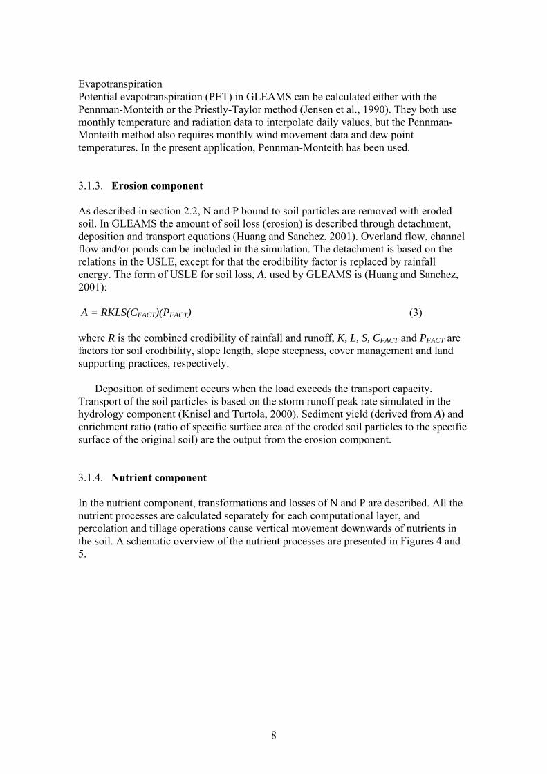
Evapotranspiration Potential evapotranspiration (PET) in GLEAMS can be calculated either with the Pennman-Monteith or the Priestly-Taylor method (Jensen et al., 1990). They both use monthly temperature and radiation data to interpolate daily values, but the Pennman-Monteith method also requires monthly wind movement data and dew point temperatures. In the present application, Pennman-Monteith has been used. 3.1.3. Erosion component As described in section 2.2, N and P bound to soil particles are removed with eroded soil. In GLEAMS the amount of soil loss (erosion) is described through detachment, deposition and transport equations (Huang and Sanchez, 2001). Overland flow, channel flow and/or ponds can be included in the simulation. The detachment is based on the relations in the USLE, except for that the erodibility factor is replaced by rainfall energy. The form of USLE for soil loss, A, used by GLEAMS is (Huang and Sanchez, 2001): A = RKLS(CFACT)(PFACT) (3) where R is the combined erodibility of rainfall and runoff, K, L, S, CFACT and PFACT are factors for soil erodibility, slope length, slope steepness, cover management and land supporting practices, respectively.

Deposition of sediment occurs when the load exceeds the transport capacity. Transport of the soil particles is based on the storm runoff peak rate simulated in the hydrology component (Knisel and Turtola, 2000). Sediment yield (derived from A) and enrichment ratio (ratio of specific surface area of the eroded soil particles to the specific surface of the original soil) are the output from the erosion component. 3.1.4. Nutrient component In the nutrient component, transformations and losses of N and P are described. All the nutrient processes are calculated separately for each computational layer, and percolation and tillage operations cause vertical movement downwards of nutrients in the soil. A schematic overview of the nutrient processes are presented in Figures 4 and 5.

9

Runoff, leaching

Runoff, leach, sed

80% of MN

20% of MN

Fresh Organic N N uptake in Plants

Fixated N

Nitrate N

Fertiliser N

Ammonia N (AMON) Atmospheric N

Potentially Mineralisable N

(POTMIN) Stable Soil N(SOILN) Organic N in

Manure (ORGNW)

Figure 4 Nitrogen pools and transformations in GLEAMS (adapted from Knisel et al., 1993)

25% of MN

75% of MN

Runoff, leaching, sediment

Fresh Organic P P uptake in plants Fertilizer P

Labile P(PLAB)

Organic P in Manure

(ORGPW) Stable Soil P

Active Organic P (humus)

Active Inorganic P

(SORGP)

Figure 5 Phosphorous pools and transformations in GLEAMS (adapted from Knisel et al., 1993)

10

Soil water and temperature factors Several transformation processes of N and P between different pools are regulated by soil water content and temperature. This is accounted for in GLEAMS through the daily calculation of soil water and temperature factors. Different soil processes include slightly different factors. One unit less factor which is used in many processes is the so called soil water factor for ammonification, SWFA, (Knisel et al., 1993) expressed as:

WPFCWPSWSWFA

−−

= SW≤ FC (4)

where SW is the actual soil water content, WP is the water content at wilting point and FC is the field capacity. They are all expressed in cm3 cm-3. The unit less temperature factor for ammonification, (TFA) is also used in several processes:

)312.095.9exp( TTTTFA−+

= TFA = 0 if T < 0 (5)

where T is the soil temperature (°C) in each layer (Knisel et al., 1993). The soil temperature is estimated by the model, based on average temperatures and solar radiation. Mineralization In GLEAMS, mineralization occurs from manure and crop residue. Nitrogen is also mineralized from potentially mineralizable N (POTMIN), while P is mineralized from organic humus phosphorous (SORGP). The mineralization rate of manure, AWMN, (kg ha-1 day-1) is given by:

AWMN = ORGNW CNP AWRC (SWFA TFA)0.5 (6) where ORGNW is the organic N in manure, CNP is a C:N and C:P ratio factor and AWRC is the manure residue composition given in ratio per day (Knisel et al., 1993). N from manure is either routed to the ammonia pool, AMON, where it might undergo nitrification to the nitrate pool. or to POTMIN. P from manure is either mineralized to the labile P pool, PLAB or routed to SORGP. The mineralization of N and P in crop residue follows the same pattern as that for mineralization of manure.

Mineralization of N, MN (kg ha-1 day-1), from POTMIN to AMON is estimated as MN = CMN POTMIN (SWFA TFA)0.5 (7)

where CMN is the specific mineralization rate constant (Knisel et al., 1993). From AMON, nitrogen is nitrified in a zero-order process, meaning that the amount of ammonia does not influence the rate of nitrification. Nitrification, NIT (kg ha-1 day-1) is calculated as:

SOILMSSWFNTFNNIT = (8)

11

where TFN is the temperature function for nitrification on the specific day, SWFN is the soil water factor for nitrification on the specific day, and SOILMS is the mass of the soil per ha (Knisel et al., 1993).

The mineralizable fraction of SORGP is governed by the relation of active N to stable N, and thus the amount of P mineralized from SORGP (kg ha-1 day-1) is expressed as:

( ) 5.0TFASWFASOILN

POTMINSORGPCMNPMN = (9)

where SOILN is the amount of N in the stable nitrogen pool (Knisel et al., 1993). Losses of N and P GLEAMS simulates losses of nitrate, ammonium and dissolved P to groundwater, and runoff of ammonia and P adsorbed to particles to surface water. Volatilization of ammonia and denitrification are also accounted for. Below is a description of denitrification of NO3 and sediment transport of P.

Denitrification occurs when soil water content exceeds field capacity. In GLEAMS, denitrification, DNI (kg ha-1), is described as a first-order process with the rate depending on soil carbon content, temperature and soil water content (Knisel et al., 1993). An increase in temperature leads to a faster denitrification with the rate of increase decreasing exponentially at high temperatures. Denitrification begins when soil water is above field capacity with 10% of the difference between saturation and field capacity, and the rate increases until the soil is saturated.

Phosphorous is adsorbed to the soil, and transported with suspended particles in runoff water. The amount of P from the manure pool, the active mineral P, the stable mineral P and from the organic humus P pool that will be transported with sediment is the product of the sediment mass, enrichment ratio and the amount of P in the respective pool. Also P from PLAB can adsorb to particles and be transported with sediments. The concentration of adsorbed labile P, Cs, is in GLEAMS dependent on the amount of clay in the soil layer. The amount of particulate P from PLAB carried away through runoff is then given as a product of sediment mass, enrichment ratio and Cs. The total amount of P transported in the sediment through runoff is the total sum of particulate P transported from all pools. Similar processes also take place for the adsorption of ammonia onto clay particles. Sediment transport only occurs for the soil in the surface computational layer (Knisel et al., 1993). Management The management practices that can be represented are sowing and harvesting of different crops, fertilization and different soil tillage operations. Several crops, types of fertilizer and tillage methods can be selected from the GLEAMS database, but they can also be customized by the user. Among other things, the crop parameters influence the N and P uptake, with the daily uptake being in proportion to the leaf area index on that day, and the availability of water and nutrients. Applied fertilizer and manure (defined as animal waste in GLEAMS) are inserted directly into the respective pool (available N

12

or P, manure N or P) to the depth of application. Tillage incorporates and mixes crop residue, manure and nutrients into the soil.

3.2. EXPERIMENTAL DATA AND MEASUREMENTS 3.2.1. Site description The studied site is situated in Shiba Village in Nanjing (32ºN, 119ºE). Shiba Village has a total of 55 ha of arable land of which 35 ha are used for vegetable production. A typical farmer has 0.2 ha of land (Huang et al., 2005). The studied field is situated on a flat plain.

Shiba Village is a peri-urban area with intense vegetable farming of 3-5 harvests per year, which was formerly used for rice cropping. In contrast to the general Chinese trend of decreasing use of manure, the amount of applied cow manure is high, in average 133000 kg ha-1 yr-1 fresh weight (Huang et al., 2005). This can be linked to the dairy farms in the vicinity from where manure can be obtained.

Two small field plots situated at a distance of 150 meters from each other were used in this study for parameterization and calibration of the GLEAMS model (Table 1).

Table 1 Plot overview

Plot

Size (m)

Area (m2)

Owner

Crop rotation

A

50 x 2.6 130

Chen Koubao

Tomato-celery-spinach B

35 x 2.0

70

Sun Huabing

Tomato-celery-spinach

3.2.2. Climate data The mean annual rainfall in Shiba is 1100 mm, which concentrates mainly in the period May to July. The temperature varies from a minimum of –7 ºC in January to a maximum of +40 ºC in July (Huang et al., 2005). For the simulations, climate data for Nanjing (mean monthly temperature, wind speed, dew point temperature, radiation and daily rainfall) was obtained from Nanjing Meteorological Institute for the period of August 2003 to July 2004. The climate station is located 7.6 km from the studied fields. 3.2.3. Soil texture and hydraulic properties The soil is classified as an Udic Alfisols (USDA) with a clay loam or loam texture (Huang et al., 2005). In Appendix B, the soil hydraulic properties are shown.

13

3.2.4. Measurements of water content and N and P in soil Measured N, P and water content in the soil and the harvested crops are presented in Appendix B. Soil samples were taken down to 40 cm depth on 6 occasions from February to November, 2004. 3.2.5. Crop management data and harvest The crop management was recorded by the farmers of the respective plots and is shown in Tables 2 and 3. Soil tillage was only recorded for one occasion on Plot A, on July 17, 2004, and on two occasions on Plot B, July 20 and August 8, 2004, but the application of cow manure involves turning of the soil (Berg and Liew, 2005).

Table 2 Recorded crop management for Plot A (amounts in kg ha-1)

Amount applied Crop Date of Planting

Date of Harvest

Amount of Harvest7

Date of Application N P

Celery

2003-08-22

2003-10-09 to 10-15 34769 2003-08-071 231.1 77.3

2003-08-271 46.2 15.5 2003-09-062 53.6 0 2003-09-123 120.0 18.4 2003-09-262 53.6 0 2003-09-272 178.5 0 2003-09-292 89.2 0

Spinach 2003-10-16

2003-12-02 to 12-05 8846 2003-10-184 15.4 10.8

Tomato 2004-02-22

2004-05-01 to 06-25 719236 2003-12-265 552.1 331.3

Σ applied:

1340

453

1As pig manure 2As urea 3As human faeces 4As NPK 5As cow manure 6Edible + non edible 7Fresh weight

Table 3 Recorded crop management for Plot B (amounts in kg ha-1)

Amount applied Crop Date of Planting

Date of Harvest

Amount of Harvest6

Date of Application N P

Celery 2003-08-24

2003-10-07 to10-08 21429 2003-08-211 107.1 75.0

2003-09-052 74.3 11.4 2003-09-142 59.4 9.1 2003-09-233 132.6 0

Spinach 2003-10-11

2003-11-18 to 11-25 12214 2003-10-013 132.6 0

Tomato 2004-02-17

2004-05-13 to 07-08 315005 2004-02-164 512.7 306.7

2004-04-112 22.3 34.3

Σ applied:

1041

436.5

1As NPK 2 As human faeces 3As urea 4As cow manure 5Edible + non edible 6Fresh weight

14

3.3. MODEL APPLICATION The GLEAMS model was first applied to Plot A where the model parameters were adjusted to measurements of soil water and nutrient content as well as crop nutrient uptake. The achieved parameter setting, but with plot specific management data, was then used on Plot B. A scenario with reduced fertilizer input was applied to Plot A. The model results were also evaluated by means of statistics and mass balance calculations.

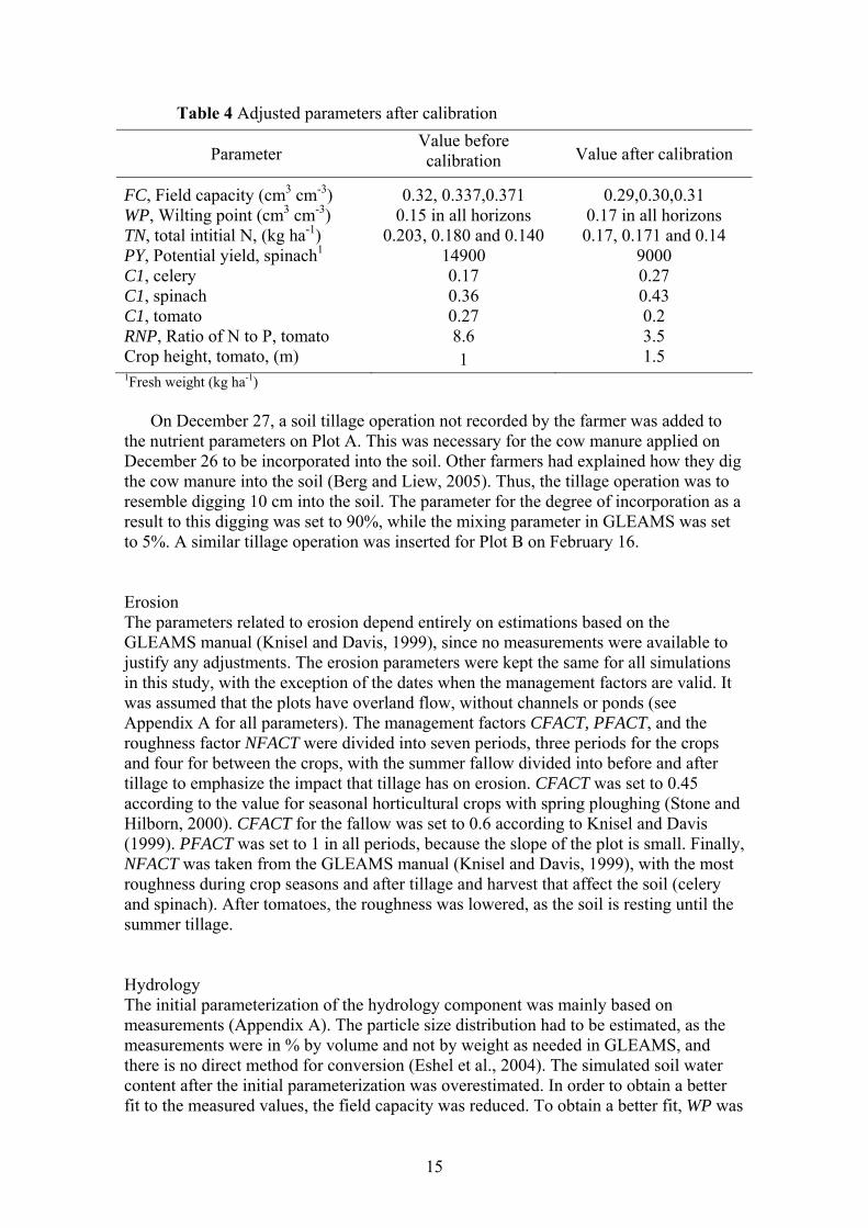
In all applications of the model, management and climate data that had been obtained for the period of August 2003 to July 2004 were used. For the calibration, unfortunately only measurements of soil water and N and P content from February to November 2004 were available. As a consequence, only the period from February to July 2004 could be directly compared with the simulations. In the simulations, the one year of recorded management and climate was repeated for 10 years to obtain results for a longer period. The reason for this is that the uncertain initial conditions may influence the results significantly, so the model was evaluated for the third year of the simulation. The reason for simulating additional years is that potential long term effects of changes in N and P pools can be observed. The simulation period was arbitrarily chosen to be 1995-2004, and the year observed for comparison with measurements was then chosen to be 1997. 3.3.1. Parameterization and calibration The initial parameterization was based on the measurements (Appendix B) and the recorded management (Tables 2 and 3) on the two plots. Other parameters were estimated using the GLEAMS manual (Knisel and Davis, 1999). In Table 4, the adjusted parameters after calibration are presented. For an overview of all parameters, see Appendix A. After the initial parameterization, the model was calibrated for Plot A by comparing simulated output to plot specific measurements from 2004. First, the water content in the different soil layers was calibrated. Then the nitrogen, nitrate and ammonia contents of the soil layers were calibrated for the nutrient part of the model. Erosion was not calibrated, as there were no measurements of erosion. The calibration process was iterative, and aimed at minimizing the difference between simulated and measured values. This was simply done by plotting the modelled and measured values in the same graphs. Considering the relatively few measurements available and the short period of simulation, a more elaborate statistical approach would not have a significant value.

Simulations for Plot B were performed using the calibrated parameters for Plot A, unless specified differently below. Management The dates for management were inserted into the model for one year of crop rotation (three different crops). This rotation begins on January 1 and ends on December 31, with the management recorded in spring 2004 entered until July 31, and the management from autumn 2003 entered from August 1.

15

Table 4 Adjusted parameters after calibration

Parameter Value before calibration

Value after calibration

FC, Field capacity (cm3 cm-3) 0.32, 0.337,0.371 0.29,0.30,0.31 WP, Wilting point (cm3 cm-3) 0.15 in all horizons 0.17 in all horizons TN, total intitial N, (kg ha-1) 0.203, 0.180 and 0.140 0.17, 0.171 and 0.14 PY, Potential yield, spinach1 14900 9000 C1, celery 0.17 0.27 C1, spinach 0.36 0.43 C1, tomato 0.27 0.2 RNP, Ratio of N to P, tomato 8.6 3.5 Crop height, tomato, (m) 1 1.5

1Fresh weight (kg ha-1)

On December 27, a soil tillage operation not recorded by the farmer was added to the nutrient parameters on Plot A. This was necessary for the cow manure applied on December 26 to be incorporated into the soil. Other farmers had explained how they dig the cow manure into the soil (Berg and Liew, 2005). Thus, the tillage operation was to resemble digging 10 cm into the soil. The parameter for the degree of incorporation as a result to this digging was set to 90%, while the mixing parameter in GLEAMS was set to 5%. A similar tillage operation was inserted for Plot B on February 16. Erosion The parameters related to erosion depend entirely on estimations based on the GLEAMS manual (Knisel and Davis, 1999), since no measurements were available to justify any adjustments. The erosion parameters were kept the same for all simulations in this study, with the exception of the dates when the management factors are valid. It was assumed that the plots have overland flow, without channels or ponds (see Appendix A for all parameters). The management factors CFACT, PFACT, and the roughness factor NFACT were divided into seven periods, three periods for the crops and four for between the crops, with the summer fallow divided into before and after tillage to emphasize the impact that tillage has on erosion. CFACT was set to 0.45 according to the value for seasonal horticultural crops with spring ploughing (Stone and Hilborn, 2000). CFACT for the fallow was set to 0.6 according to Knisel and Davis (1999). PFACT was set to 1 in all periods, because the slope of the plot is small. Finally, NFACT was taken from the GLEAMS manual (Knisel and Davis, 1999), with the most roughness during crop seasons and after tillage and harvest that affect the soil (celery and spinach). After tomatoes, the roughness was lowered, as the soil is resting until the summer tillage. Hydrology The initial parameterization of the hydrology component was mainly based on measurements (Appendix A). The particle size distribution had to be estimated, as the measurements were in % by volume and not by weight as needed in GLEAMS, and there is no direct method for conversion (Eshel et al., 2004). The simulated soil water content after the initial parameterization was overestimated. In order to obtain a better fit to the measured values, the field capacity was reduced. To obtain a better fit, WP was

16

increased. However, when WP was set to greater than 0.17, the rate of decomposition of cow manure became unrealistic, with all organic N mineralized in one day. Therefore, WP was not raised higher, but left at 0.17. Probably, increasing WP disturbed the SWFA or other soil water factors (section 3.1) which affected the nutrient processes. This illustrates the importance of the soil water factors for the simulation of nutrient processes. Nutrients To simulate the correct nutrient export with the yield, three crop parameters (potential yield, PY, the nitrogen content coefficient, C1, and the ratio of N to P, RNP) were adjusted until the N and P amounts in the simulated yield, as well as the biomass yield, corresponded with the crop analysis measurements and the registered yield. Because of a lower registered yield of tomato and celery on Plot B, the potential yield of these crops were lowered compared to Plot A, while the potential yield of spinach was increased to correspond with the larger harvest on Plot B (Table 3).

The initial total nitrogen content in the soil was set on both plots so that the simulation on the third year of simulation matched the measurements of total N (Appendix B) on the respective plot. Then, the NH4 and NO3 content were calibrated against measurements through an increase of the specific mineralization rate constant, CMN, from 0.001 to 0.016 according to Webb et al. (2001). Parameters that were investigated, but where modification gave little effect on the simulation were porosity, (POR) and POTMIN. These parameters were finally left unchanged. The parameters for incorporation and mixing of cow manure were also modified without any effect on the content of inorganic N. The effects of decreasing the immobilization of nitrate and increasing the decomposition of crop residue were also investigated, but abandoned. Another theory was that the nitrate in irrigation water could influence the nitrate content in the soil. Thus, extra fertilization was added on the days of irrigation, but the effects were neglible so also this was discarded.

The initial values of total phosphorous were set so that the simulated P content in February 1997 agreed with the measured P content of February 9, 2004.

3.3.2. Scenario for Plot A A scenario was constructed for Plot A, with reduced input of manure and fertilizer (Table 5). The intention with the scenario was to decrease the input of N and P without reducing the yield.

17

Table 5 The changed fertilizer input in the Scenario for Plot A, kg ha-1

Date and type of manure/fertilizer

Actual amount applied on Plot A

Amount applied in the Scenario

August 7, Pig manure1 7731

4947 September 26, Urea2 53.4 0 September 27, Urea2 178.5 89.2 December 26, Cow manure1 33461 21415

Total N applied 1339 915 Total P applied 453 306

1Dry weight 2NH4-N 3.3.3. Investigation of CN The curve number, CN, is of great importance for the partitioning of water between surface runoff and infiltration in GLEAMS, and should be chosen with care (Muller and Gregory, 2003). In this application a CN of 83 was chosen from the GLEAMS manual (Knisel and Davis, 1999) based on the relatively high clay content (46 %), which places the soil in hydrologic group C (Knisel and Davis, 1999). Because there is little observation of surface runoff and the saturated hydraulic conductivity (Appendix B) is rather high, the lowest CN for group C was then chosen. However, this choice is quite uncertain and therefore two extra simulations with CN set to 53 and 93 were performed. The effects on soil water, nitrogen and phosphorus content, as well as N and P losses were observed. 3.3.4. Model evaluation Statistical analysis To compare the calibration results with the simulation output before calibration, a brief statistical analysis was made for the period of February 9 to July 12. As the autumn measurements are from a later year (see the introduction of section 3.3) they were not included. The analysis was made through an adjustment of the Nash-Sutcliffe (1970) model efficiency (EF)

2

1

1

22

1

)(

)()(

∑

∑∑

−

−−−= N

NN

OO

OPOOEF (11)

where O is the observed or measured value, O is the mean of observed values from 1 to N, and P is the estimated or simulated value. An EF of 1.0 means a perfect fit, while a negative result indicates a poor fit of simulated values to measurements. Normally, EF is calculated for continuous series and not for such few measurements as in this application. To account for the variability in time (simulated values occurring some days before or after the measurement), the simulated values used in the analysis is the average of results from 3 days before and after the date of measurement. It was believed

18

that this would give a more reliable analysis, although in some cases the result could be a worse fit than actual. Because of these uncertainties, EF is only used for comparison between parameter settings and not as an absolute indicator of model fit. Mass balance A mass balance estimation of nitrogen was performed on Plot A from December 25 to March 31. The purpose of this mass balance estimation was to achieve a better understanding of the partitioning and dynamics of the decomposition of the large amount of cow manure applied December 26. The changes in the simulated N pools from December 25 to January 31 and to March 31 were compared with the changes in measured NO3 and NH4 contents in the soil from December 25 to February 9 and to March 24. Since the GLEAMS output cannot present daily crop N uptake, but only monthly, the simulated pools do not exactly correspond to the measured in time. The initial amounts of nitrate and ammonia in the soil on December 25 were estimated through interpolation from the measurement on November 9 to the measurement on February 9, since there was no measurement on December 25. The applied cow manure was the only source of N during this period, except for negligible amounts of N in rainfall.

Another mass balance estimation was performed of the total N and P input and losses for the 10 year simulation period, in order to compare the effects of different management on Plot A, Plot B and the scenario on Plot A. 4. RESULTS AND DISCUSSION In the results presented below, the simulated values are compared to measurements. However, only the period from February to July can be considered for a correct comparison, because the September and November measurements were taken one year later (see section 3.3). Although the autumn values cannot be directly compared, these measurements can serve as an indicator of the model behaviour, since the management was similar for the two years

4.1. SOIL WATER CONTENT The simulated soil water content for Plot A before and after calibration, and for Plot B are presented in Figures 6 and 7. As can be seen in Figure 6, reduction of FC and WP resulted in generally lower soil water content, and an increase of the crop height of tomatoes reduced the water content in the two top layers in February and March. The simulated water content in the top layer (0-18 cm) had a delay of 1-2 weeks compared to the measured values in February and July, and the model could not reproduce the decrease in water contents in July in the bottom layers. The EF-value improved from -7.9 to -6.2 as a mean of the three layers (Table 6), which indicates improved simulated values after lowering FC. The FC and the WP has also been calibrated in many previous applications with GLEAMS (e.g. Shirmohammadi et al., 1998; Knisel and Turtola, 2000). Consequently, the poor simulated dynamics of soil water content might be a result of FC not having an exact physical meaning in the model, or of the functional storage-routing approach for water flows, where all the water above FC in a layer is

19

routed to the next layer in one day. The lack of description for upward capillary movement of water might be another reason for the poor simulations. Many model applications do not consider the day to day soil water content, but present monthly or yearly measurements of accumulated percolation and runoff, which are also the components on which the GLEAMS hydrology component has been validated (Knisel, 1993; Muller and Gregory, 2003).

Table 6. EF-values for the content of water, NO3 and NH4 in the soil for Plot A and B. For Plot A, EF-values are presented both before and after calibration and for the different CN . This is to see any improvements from before to after calibration.

Soil water content Soil NO3 content

Soil NH4 content

Soil profile depth (cm) 0-18

18-26

26-40 0-18

18-26

26-40 0-18

18-26

26-40

Plot A before calibration -4.4 -5.6 -13.6 -2.3 -6.4 -11.5 0.7 -0.4 -0.6

Plot A after calibration -2.3 -6.5 -9.7 -2.1 -2.7 -3.9 0.7 -0.5 -0.6

Plot B -4.7 -28 -16.4 -0.2 0.6 -1.3 -443 -29.5 -18.8 Plot A, CN =53 -2.1 -6.6 -8.6 Plot A, CN =93 -1.6 -6.5 -17.5

4.2.NUTRIENT UPTAKE Table 7 shows the measured and simulated yields for the different crops. After calibration, the simulated N and P content in the yields were close to the measured values. The total simulated N removal with the harvest was 287 kg ha-1 yr-1, which is an overestimation with c. 3%, and for P the simulated removal was 70 kg ha-1 yr-1, which is close to the measured 71 kg ha-1 yr-1.

Table 7 Simulated and measured yield and the amount of N and P exported with the harvest (kg ha-1) on Plot A

Tomato

Celery Spinach Measured

Simulated Measured Simulated Measured Simulated

Biomass1 71923 64580 34769 40000 8846 9000 N in yield 135 142 106 107 39 39 P in yield 39 39 26 24 6 7

1Fresh weight

20

a) Soil water content 0-18 cm

14

16

18

20

22

24

26

28

30

32

JanFeb

MarApr

MayJun

JulAug

SepOct

NovDec

Soil

wat

er (%

of v

olum

e)

b) Soil water content 18-26 cm

14

16

18

20

22

24

26

28

30

32

34

JanFeb

MarApr

MayJun

JulAug

SepOct

NovDec

Soil water (%

of v

olum

e)

c) Soil water content 26-40 cm

13

18

23

28

33

38

JanFeb

MarApr

May

JunJul

AugSep

OctNov

Dec

Soil water (%

of v

olum

e)

Figure 6 Simulated, before and after calibration, and measured soil water

content (% of volume) for each soil layer on Plot A. The results are presented for the third year of the simulation period.

Measured Measured other year (indicator)

Simulated after calibrationSimulated before calibration

21

a) Soil water content 0-18 cm

16

18

20

22

24

26

28

30

32

JanFeb

MarApr

MayJun

JulAug

SepOct

NovDec

Soil

wat

er (%

of v

olum

e)

b) Soil water content 18-26 cm

16

18

20

22

24

26

28

30

JanFeb

MarApr

MayJun

JulAug

SepOct

NovDec

Soil water

(% of v

olum

e)

c) Soil water content 26-40 cm

16

18

20

22

24

26

28

30

32

34

JanFeb

MarApr

MayJun

JulAug

SepOct

NovDec

Soil water

(% of v

olum

e)

Figure 7 Simulated and measured soil water content (% of volume) for each soil

layer on Plot B. The results are presented for the third year of the simulation period.

Simulated Measured Measured other year (indicator)

22

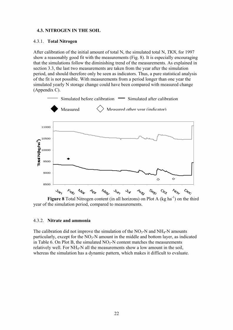
4.3. NITROGEN IN THE SOIL 4.3.1. Total Nitrogen After calibration of the initial amount of total N, the simulated total N, TKN, for 1997 show a reasonably good fit with the measurements (Fig. 8). It is especially encouraging that the simulations follow the diminishing trend of the measurements. As explained in section 3.3, the last two measurements are taken from the year after the simulation period, and should therefore only be seen as indicators. Thus, a pure statistical analysis of the fit is not possible. With measurements from a period longer than one year the simulated yearly N storage change could have been compared with measured change (Appendix C).

8500

9000

9500

10000

10500

11000

Jan FebMar

AprMay

Jun Jul AugSep

OctNov

Dec

Tota

l N (k

g ha

-1)

Figure 8 Total Nitrogen content (in all horizons) on Plot A (kg ha-1) on the third

year of the simulation period, compared to measurements.

4.3.2. Nitrate and ammonia The calibration did not improve the simulation of the NO3-N and NH4-N amounts particularly, except for the NO3-N amount in the middle and bottom layer, as indicated in Table 6. On Plot B, the simulated NO3-N content matches the measurements relatively well. For NH4-N all the measurements show a low amount in the soil, whereas the simulation has a dynamic pattern, which makes it difficult to evaluate.

Measured Measured other year (indicator)

Simulated after calibrationSimulated before calibration

23

a) NH4-N content Plot A 0-18 cm

0

50

100

150

200

250

300

350

JanFeb

MarApr

MayJun

JulAug

SepOct

NovDec

NH 4

-N (k

g ha

-1)

b) NH4-N content Plot B 0-18 cm

0

50

100

150

200

250

JanFeb

MarApr

MayJun

JulAug

SepOct

NovDec

NH 4

-N (k

g ha

-1)

Figure 9 Simulated, before and after calibration, and measured NH4-N content

(kg ha-1) for the top horizon on Plot A and B, respectively. The results are presented for the third year of the simulation period. Simulations only gave significant concentrations in the top horizon of the soil, so the contents of the lower horizons are not presented here.

As shown in Figure 9a, on Plot A, the measured amount of NH4-N in the top soil layer was 292 kg ha-1 on February 9th, while the simulation only reached about 170 kg ha-1 for the same date. In other parts of the year, with the measured amounts below 50 kg ha-1, there was a better agreement between simulations and measurements. The measured peak in February most likely is related to the mineralization of the cow manure applied in December, as shown by the mass balance calculations for Plot A from December to March (Fig. 10). In the simulations, a great part of the N in cow manure remains as organic N during the spring: after 35 days less than 30% has been mineralized to NH4

Measured Measured other year (indicator)Simulated after calibrationSimulated before calibration

24

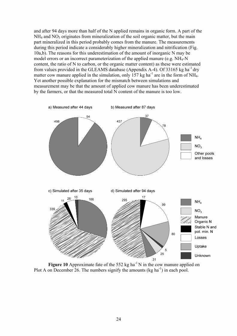
and after 94 days more than half of the N applied remains in organic form. A part of the NH4 and NO3 originates from mineralization of the soil organic matter, but the main part mineralized in this period probably comes from the manure. The measurements during this period indicate a considerably higher mineralization and nitrification (Fig. 10a,b). The reasons for this underestimation of the amount of inorganic N may be model errors or an incorrect parameterization of the applied manure (e.g. NH4-N content, the ratio of N to carbon, or the organic matter content) as these were estimated from values provided in the GLEAMS database (Appendix A-4). Of 33165 kg ha-1 dry matter cow manure applied in the simulation, only 157 kg ha-1 are in the form of NH4. Yet another possible explanation for the mismatch between simulations and measurement may be that the amount of applied cow manure has been underestimated by the farmers, or that the measured total N content of the manure is too low.

Figure 10 Approximate fate of the 552 kg ha-1 N in the cow manure applied on

Plot A on December 26. The numbers signify the amounts (kg ha-1) in each pool.

25

The reason for the severely underestimated NH4-N amount in the middle and bottom layers could probably be partly explained by an over estimation of the soil water content in these layers. Since water content remains at FC most of the simulation period (Fig. 6), the nitrification will be at an optimum rate (equation 8). Consequently, all the ammonia in these layers is converted to nitrate.

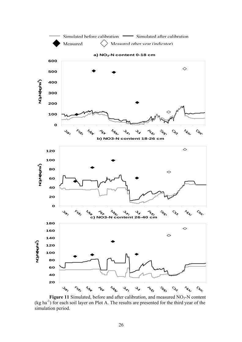
The simulations of NO3-N show an even greater discrepancy between simulated and measured amounts than for NH4. As shown in Figure 11, the measured amount of NO3-N in the top soil layer of Plot A increased from100 kg ha-1 in February to about 500 kg ha-1 in April. The reason for this large increase was mineralization and nitrification of the manure applied in December (Fig 10), and of some soil organic matter. This increase was coupled to a decrease in NH4-N from c. 300 to 35 kg ha-1 (Fig 9a). The model could not mimic the pattern of measured NO3-N in the top soil layer from February to April: the amount of NO3-N was only increased with about 50 kg ha-1. The NO3-N on Plot B shows a similar pattern (Fig. 12). At first, this was thought to be directly related to the low mineralization rate in the simulations and the low amount of NH4-N, as explained above. However, in GLEAMS, the nitrification from NH4 to NO3 is not related to the amount of NH4 in the soil, but is decided by soil water content, temperature and soil mass (equation 8). Thus, the underestimation of NO3 in the soil could be caused by unreliable simulations of soil water and/or temperature, or errors in the estimation of soil mass. Other NO3 related processes, which may be indirectly linked to mineralization, like immobilization, might also have an impact on the simulated NO3 amounts.

Indirect effects of mineralization on NO3-N content are seen from the calibration results, which show that the calibration of the mineralization factor, CMN lead to a 62% increase in the amount of NO3 in the soil. Other examined ways to increase the soil NO3 amounts were not successful, for example to decrease the immobilization factor; increase the crop residue decomposition; add more nitrate fertilizer to simulate nitrate in irrigation water; increase the initial amount of nitrate in the soil and the potentially mineralizable N; change the porosity; and to increase the incorporation depth of the cow manure. Hence, indirect effects of an erroneous mineralization are probably one of the most plausible explanations to the underestimations of NO3-N. Mineralization problems have also been reported by other authors. Dukes and Ritter (2000) obtained a simulated mineralization by GLEAMS of 64.8 kg ha-1 yr-1, compared to a measured mineralization of 208 kg ha-1 yr-1. Knisel et al.(1993) mention that sometimes there can be a general underestimation of NO3 concentration, because of a tendency to underestimate the mineralization during cooler periods.

26

a) NO3-N content 0-18 cm

0

100

200

300

400

500

600

JanFeb

MarApr

MayJun

JulAug

SepOct

NovDec

NO

3-N (k

g ha

-1)

b) NO3-N content 18-26 cm

0

20

40

60

80

100

120

JanFeb

MarApr

MayJun

JulAug

SepOct

NovDec

NO

3-N (k

g ha

-1)

c) NO3-N content 26-40 cm

20

40

60

80

100

120

140

160

180

JanFeb

MarApr

MayJun

JulAug

SepOct

NovDec

NO

3-N (k

g ha

-1)

Figure 11 Simulated, before and after calibration, and measured NO3-N content (kg ha-1) for each soil layer on Plot A. The results are presented for the third year of the simulation period.

Measured Measured other year (indicator)Simulated after calibrationSimulated before calibration

27

a) NO3-N content 0-18 cm

20

70

120

170

220

270

JanFeb

MarApr

MayJun

JulAug

SepOct

NovDec

NO

3-N (k

g ha

-1)

b) NO3-N content 18-26 cm

20

30

40

50

60

70

80

JanFeb

MarApr

MayJun

JulAug

SepOct

NovDec

NO

3-N (k

g ha

-1)

c) NO3-N content 26-40 cm

30

40

50

60

70

80

90

100

110

120

JanFeb

MarApr

MayJun

JulAug

SepOct

NovDec

NO

3-N (k

g ha

-1)

Figure 12 Simulated and measured NO3-N content (kg ha-1) for each soil layer

on Plot B. The results are presented for the third year of the simulation period.

Simulated Measured Measured other year (indicator)

28

4.4. PHOSPHORUS 4.4.1. Total P Due to a lack of accurate measurements of total P (TP) content, TP could only be calibrated against the measurement in February. The initial values were set so that the simulated TP on February 9, 1997 corresponds with the measured TP on February 9, 2004 (Fig. 13). Long-term accumulation of P is shown in Appendix C.

8000

8200

8400

8600

8800

9000

9200

9400

9600

Jan FebMar

AprMay

Jun Jul AugSep

OctNov

Dec

Tota

l P (k

g ha

-1)

Figure 13 Total Phosphorus content on Plot A kg ha-1 on the third year of the

simulation period, compared with measurements

4.5. TESTING OF DIFFERENT CN Changing the curve number, CN, and thus the partitioning between surface runoff and infiltration, did not have a significant impact on the water and nutrient contents of the soil. Lowering the curve number from 83 to 53 (increasing the part of rainfall going to infiltration) only slightly decreased the NO3-Ncontent, with a 5-20 kg ha-1 decrease of in the bottom horizon during the rainy part of the summer, i.e. July and August, and resulted in a slightly greater accumulation of phosphorus (100-130 kg ha-1 year-1 more), during the last years of the simulation period, while PO4-P and NH4-N did not change.

Setting CN to 93 (increasing the part of rainfall becoming runoff) did not result in

any significant change of the soil water content, except for the bottom layer being somewhat drier during early spring and in May. The dynamics of the NO3-N content in soil remained the same, but the level was 5 to 6 kg ha-1 higher. In the middle and bottom layers, the NO3-N content increased with up to 30 kg ha-1 in July and August, while there was little impact on NH4-N. The amount of TP decreased with 100 to 150 kg ha-1 yr-1 during the last years of the simulation period, while PO4-P and NH4-N did not change remarkably.

Measured Measured other year (indicator) Simulated after calibrationSimulated before calibration

29

Although the different CN-values only resulted in small differences in soil water and nutrient contents, there was a clear change in the distribution of nutrient losses due to the change in distribution of water between runoff and infiltration (Table 8). The total loss of nitrogen remained about the same, with a difference of 7 kg ha-1 year-1. On the other hand, the phosphorus losses were significantly altered by the curve number, from 6.6 kg ha-1 year-1 for CN 53 to 51.2 kg ha-1 year-1 for CN 93. If P is to be calibrated, the curve number therefore seems to be an important parameter to change. However, since different CN only resulted in small changes in the soil water and soil nutrient contents, it could be difficult to calibrate against the amounts of P in the soil.

Table 8 N and P losses resulting from simulations with different CN. The amounts are the accumulated losses after 10 years (kg ha-1 10 years-1)

CN 53

CN 83 CN 93 N P N P N P

Runoff 0.46 2.25 139 105 944 313 Sediment 17 27 76 120 110 180 Leached 5272 37 5060 30 4177 19 Denitrification 2489 - 2572 - 2560 - Volatilization 1945 - 1945 - 1945 -

Total loss

9723 66 9792 255 9736 512

4.6. COMPARISON OF N LOSSES FROM DIFFERENT MANAGEMENT PRACTICES

Table 9 shows the N balance for the simulation on Plot A and B, and for the scenario on Plot A. The same crops were grown on both plots at about the same time, but the farmer on Plot B applied the cow manure in February instead of in December. The amount of applied N was c. 20 % lower on Plot B compared to Plot A, and the harvest yield of tomato was c. 56 % lower and the harvest of celery 38 % lower on Plot B compared to Plot A (Tables 2 and 3). However, since the model indicated that there is enough nitrate in the soil for the plant, the reduction in yield was probably caused by some other management factor, for example pests, weeds or fungi. The scenario indicated that the amount of applied N could be reduced radically without any quantitative effect on the yield. In the scenario, the amount of applied N was reduced with 4430 kg ha-1 yr-1, resulting in a reduced leaching with 43 %, reduced losses to air with 33 %, and reduced accumulation in the soil with 86 %. Despite the lower applied amount of N on Plot B, GLEAMS predicted somewhat higher leaching than for Plot A. However, the leaching on Plot A was probably wrongly estimated since the nitrate amount in the soil is underestimated during large parts of the year. Without measurements on the actual leaching, it is hard to tell how accurate the leaching predictions are.

The simulated erosion on Plot A was 681 kg ha-1 yr-1, whereas Plot B had a simulated soil loss of 7474 kg ha-1 yr-1. This is somewhat surprising, considering that the erosion parameters were almost the same, except for the dates of planting and harvesting, and the size of the plot. On Plot B there was also one more occasion with tillage than on Plot A.

30

Table 9 N balances for 10 years of simulation. The amounts are the average annual accumulated values (kg ha-1 year-1)

Nitrogen flow

Plot A Plot A, scenario Plot B

N applied with manure 949 667 669 N applied with fertilizer 390 247 372 N input from rain 7 7 7

Σ N input to the soil

1346 922 1048

Crop uptake N 285 284 185 Runoff of NO3-N 1 1 2 Runoff of NH4-N 13 10 17 Sediment loss N 8 6 34 Leached N 506 287 581 Denitrification NO3-N 257 150 226 Volatilization of NH4-N 195 154 76

Σ N removed from soil

1265 892 1121

Balance in the soil +81 +30 –73 Nutrient efficiency1 21% 31% 17%

1Crop N uptake divided with total N input

4.7. SUMMARY OF THE DISCUSSION AND SUGGESTIONS FOR THE USE OF THE GLEAMS MODEL

There are a number of factors that may have influenced the sometimes poor fit between the simulations and the measurements: an inappropriate parameter setting, errors in the measurements, and incorrect process descriptions in the model.

The chosen values of several parameters, especially those in the erosion component, are uncertain. However, an erroneous parameter setting for the erosion would mainly affect the P losses, while the impact on the nitrogen probably would be considerably smaller. In the hydrology component, the parameters influencing water flows and the SWFA (i.e. FC and WP) may have an impact on the nutrient processes. Other important parameters in this application are those connected to mineralization of manure, such as the rate constants for mineralization and immobilization.

The recorded management may include errors; especially sensitive are probably the irrigation amounts and the applied amounts of manure and fertilizer. There are also very few soil measurements to calibrate against, and any errors in these could be difficult to identify. For example for total P, there was a remarkable increase of measured P during a period when no P was added. However, for NO3-N in the uppermost layer on Plot A (Fig. 11), three consecutive measurements indicate a high NO3 concentration, which contradicts measurement errors as the reason for poor simulations of inorganic N in the soil.

Another limitation of the model application is the availability of data. The lack of

complete measurements of nutrient content in manure may have affected the results,

31

since the input of manure is so high. An erroneous estimation might thus have a great impact on the simulation output. There was only climate and management data from one year, and initialization data (e.g. soil water content, and complete N and P pools) are lacking. Climate and management data for the previous years would perhaps have helped in minimizing any effects on the soil remaining from previous years. However, in the current application, the spring simulation, used for comparison between simulated and measured values, is preceded by six months of actual climate and management. This increases the reliability of the simulated conditions during the spring. Another aspect of using the spring for comparison is that there was a heavy manure application in late December, which probably had a higher effect on the inorganic nitrogen content in the spring than any previous events. However, the initial contents of the more stabile pools, which may affect mineralization, remain unknown.

The lack of dynamics of the soil water content has been mentioned as one probable reason for the poor simulations of the mineral nitrogen amounts in the soil. Another issue that has been discussed is the mineralization. It might be speculated that the GLEAMS model in its current shape is not suitable for intensive cropping systems with a high input of manure. Since the model contains a number of empirically derived constants, it may not be directly applicable on all farming systems. Therefore, the model probably needs a more thorough parameterization, calibration and validation before it can be used with confidence in the Shiba village.

Hence, are the results good enough for evaluating different BMPs at the Shiba

village? This depends on the measures applied for reducing the losses. The mineralization in the simulation releases inorganic nitrogen in the summer instead of spring, a delay that may have consequences. For example, a scenario with a cover crop in the summer could seem to reduce the nitrogen leaching, but since it is not certain how much nitrogen that has leached before the summer, the predictions would be uncertain. On the other hand, a scenario with reduced N application in the winter/spring would probably be reliable, as long as the nitrogen content is enough for the plant uptake. However, in reality, a larger reduction than estimated from simulations would be possible. Another issue to be analysed before developing scenarios is the reason for the large simulation of erosion on Plot B. If this depends on the additional tillage as compared to Plot A, then of course scenarios with modified tillage cannot be used.

5. CONCLUSIONS

- The application rate of N and P, especially in the form of manure, on the vegetable fields in Shiba village is high and considerable reductions can be made without affecting the yield. How to reduce the input of N and P can be determined by the use of a simulation model, such as GLEAMS.

- The calibration of nitrogen simulations with the GLEAMS model was only partly successful, mainly due to difficulties in increasing inorganic N levels in the soil. The results indicate that parameters related to the decomposition of manure need further calibration, or that the empirically based constants in the model need to be adjusted.

- According to the current GLEAMS simulation, the N application could be reduced from 1339 kg ha-1 to 915 kg ha-1 without any effect on the yield.

32

6. REFERENCES Berg, J. and Liew, J., (2005). Participatory Methods for Scenario Development for Improved N and P Use Efficiency and Parameterisation of the GLEAMS Model - a Field Study of a Small-scale, Peri-urban Vegetable Farming-system in Nanjing, China. 22.5 ECTS, Advanced Level. Minor Field Study Nr 71, Dep. of Soil Sciences, Swedish University of Agricultural Sciences (SLU). Box 7014, SE-750 07 Uppsala, Sweden. Brady, N.C. and Weil, R.R., (2002). The Nature and Properties of Soils. Pearson Education Inc., Upper Saddle River, New Jersey Cao, Z.H., Huang, J.F., Xhang, C.S. and Li, A.F., (2004). Soil quality evolution after land use change from paddy soil to vegetable land. Environmental Geochemistry and Health, 26:97-103 Djodjic F, Montas H, Shirmohammadi A, Bergstrom L and Ulen B., (2002). A decision support system for phosphorus management at a watershed scale. J Environ Qual. 31(3):937-45 Duan S.W., Xhang, S. and Huang H.Y., (2000). Transport of dissolved inorganic nitrogen from the major rivers to esturaries in China. Nutrient Cycling in Agroecosystems, 57:13-22 Dukes, M.D. and Ritter, W.F., (2000). Validation of GLEAMS nutrient component for wastewater application in the Mid-Atlantic region, Bioresource Technology 74:89-102 Eshel, G., Levy, G.J., Mingelgrin, U. and Singer, M.J., (2004). Critical Evaluation of the Use of Laser Diffraction for Particle-Size Distribution Analysis, Soil Science Society of America Journal, 68:736-743 Galloway, J.N., (2000). Nitrogen mobilization in Asia, Nutrient Cycling in Agroecosystems, 57:1-12 Gerber, P., Chilonda, P., Franceschini, G. and Menzi, H., (2002). Livestock density and nutrient balances across Asia, In: The Proceedings of the 10th International Conference of the RAMIRAN Network, Strbské Pleso, Slovak Republic May 14-18, 2002. ISBN: 80-88985-68-4 Guo, H.Y., Wang, X.R. and Zhu, J.G., (2004). Quantification and index of non-point source pollution in Taihu Lake region with GIS, Environmental Geohchemistry and Health, 26: 147-156 Huang, B., Shi, X.Z., Yu D.S., Öborn, I., Blombäck, K., Pagella, T.F., Wang H.J., Sun W.X. and Sinclair, F.L., (2005). Environmental Assessment of Small-scale Vegetable Farming Systems in Peri-Urban Areas of the Yangtze Delta River Region, China. Agriculture, Ecosystems and Environment (in press) Huang, K.-L. and Sanchez, J.F. (2001). GLEAMS – Simulation with data from the Buck Island ranch. Simulation of watershed systems, ABE 6254. http://www.agen.ufl.edu/~klc/abe6254/gleamsapp01.pdf (2005-08-08)

33

Jensen, M.E., Burman, R.D. and Allen, R.D. (Eds.) 1990. Evapotranspiration and Irrigation. Water Requirements. American Society of Civil Engineers, Manuals and Reports on Engineering Practice, No. 70. 332 pp. Jin, J. and Jiang, C. (2002). Spatial variability of soil nutrients and site-specific nutrient management in the P.R. China. Computers and Electronics in Agriculture 36, 165-172. Knisel, W. G., (1980). CREAMS: a field-scale model for chemicals, runoff and erosion from agricultural managment systems. USDA, Conservation Research Report 26 Knisel, W. G. and Davis, F.M., (1999). GLEAMS (Groundwater Loading Effects of Agricultural Management Systems) Version 3.0 User Manual. SEWRL-WGK/FMD-050199. Tifton, GA. http://www.cpes.peachnet.edu/sewrl/Gleams/glmscov1.pdf (2005-08-08) Knisel, W.G., Davis, F.M. and Leonard, R.A., (1993). GLEAMS version 2.10. USDA-ARS, Coastal Plain. Experiment Station. Southeast Watershed Research Laboratory. Tifton, Georgia, 31793 Knisel, W.G. and Turtola, E., (2000). GLEAMS model application on a heavy clay soil in Finland, Agricultural Water Management 43:285-309 McGechan, M.B. and Lewis, D.R., (2002). A review of field scale phosphorus dynamics models, Biosystems Engineering 82(4):359-380 Midmore, D.J. and Jansen, H.G.P. (2003). Supplying vegetables to Asian cities: is there a case for peri-urban production?. Food Policy 28:13-27 Muller, S. and Gregory, J., (2003). Groundwater Loading Effects of Agricultural Management Systems Version 3.0 – Calibration of the GLEAMS model for Buck Island Ranch, University of Florida, Department of Agricultural and Biological Engineering. http://www.agen.ufl.edu/~klc/abe6254/gleamsapp03.pdf (2005-06-27) Nanjing Meteorological Institute, (2004). Climate data for Nanjing for the period of August 1, 2003 to July 31, 2004. Nash, J.E. and Sutcliffe, J.E., (1970). River flow forecasting through conceptual models, Part 1-A discussion of principles. J. Hydrology 10(3): 282-290 Nehru, V. and Kraay, A., Yu X.Q., (1997). China 2020: Development challenges in the new century, World Bank, Washington D.C Norse, D., Li J., Jin L. and Z. Zhang, (2001). Environmental Costs of Rice Production in China: Lessons from Hunan and Hubei.,Aileen International Press, Bethesda Richter, J. and Roelcke, M. (2000). The N-cycle as determined by intensive agriculture – examples from central Europe and China. Nutrient Cycling in Agroecosystems 57, 33-46.

34

RURBIFARM – Project proposal. 2002. Sustainable farming at the rural-urban interface – An integrated knowledge based approach for nutrient and water recycling in small-scale farming systems in peri-urban areas of China and Vietnam. Contract no. ICA4-CT-2002-10021 Shaffer, M.J., (1995). Fate and Transport of Nitrogen – What Models Can and Cannot Do. USDA RCA III Working Paper No. 11, USDA, Agricultural Research Service Great Plains Systems Research Unit Fort Collins, Colorado http://www.nrcs.usda.gov/technical/land/pubs/wp11text.html (2005-06-23) Shirmohammadi, A., Ulen, B., Bergstrom, L.F. and Knisel, W.G., (1998). Simulation of nitrogen and phosphorus leaching in a structured soil using GLEAMS and a new submodel, “PARTLE”, Transactions of the ASAE 41(2):353-360 Stone, R.P. and Hilborn, D., (2000), Universal Soil Loss Equation – Factsheet from the Ontario Ministry of Agriculture and Food, Queens Printer for Ontario, Ontari o ISSN: 1198-712X http://www.gov.on.ca/OMAFRA/english/engineer/facts/00-001.htm (2005-06-27) Tattari, S., (2002). The use of simulation models describing surface transport of phosphorus, in: Chardon, W.J, and Schoumans, O.F. (Eds.) Phosphorus losses from agricultural soils: Processes at the field scale, COST Action 832 'Quantifying the Agricultural Contribution to Eutrophication', Alterra, Wageningen, The Netherlands. pp.88-92. United Nations Development Programme, (2004a). Human development reports – Indicators. http://hdr.undp.org/statistics/data/indic/indic_41_1_1.html (2005-03-02) United Nations Development Programme, (2004b). Human development reports - Demographic Trends. http://hdr.undp.org/statistics/data/pdf/hdr04_table_5.pdf (2005-03-02) United Nations Human Settlement Programme, (2001). Urban Environment Food, For: Istanbul+5: Reviewing and Appraising Progress Five Years After Habitat II http://www.unchs.org/Istanbul+5/72.pdf (2005-06-27) USDA-SCS (U.S. Department of Agriculture-Soil Conservation Service), (1972). SCS National Engineering Handbook: Section 4, Hydrology. Chapter 10, Estimation of Direct Runoff From Storm Rainfall. U.S. Department of Agriculture, Soil Conservation Service, Washington, D.C., pp. 10.1-10.24. Veeck, A. and Veeck, G. (2000). Consumer segmentation and changing food purchase patterns in Nanjing, PRC. World Development 28(3):457-471 Wang, X.J. and Tao, S., (1998). Spatial structures and relatations of heavy metal content in wastewater irrigated agricultural soil of Beijing’s eastern farming regions. Bulletin of Environmental Contamination and Toxicology 61:261-268 Wang, X.Y., (2003). Diffuse pollution from livestock feeding in China. In: Bruen, M. (editor) Diffuse Pollution and Basin Management. Proceedings of the 7th International Specialised IWA Conference, Dublin, Ireland. ISBN 1902277767, 4vols. 1140 pps

35

Webb, T.H., Lilburne, L.R. and Francis, G.S., (2001). Validation of the GLEAMS simulation model for estimating net nitrogen mineralisation and nitrate leaching under cropping in Canterbury, New Zealand, Australian Journal of Soil Research, 39:1015-1025 Wischmeier, W.H. and Smith, D.D., (1978). Predicting rainfall erosion losses – a guide to conservation planning. U.S. Department of Agriculture, Agriculture Handbook No. 537 Zhu, Z.L. and Chen, D.L., (2002). Nitrogen fertilizer use in China – Contributions to food production impacts on the environment and best management strategies. Nutrient Cycling in Agroecosystems 63:117-127

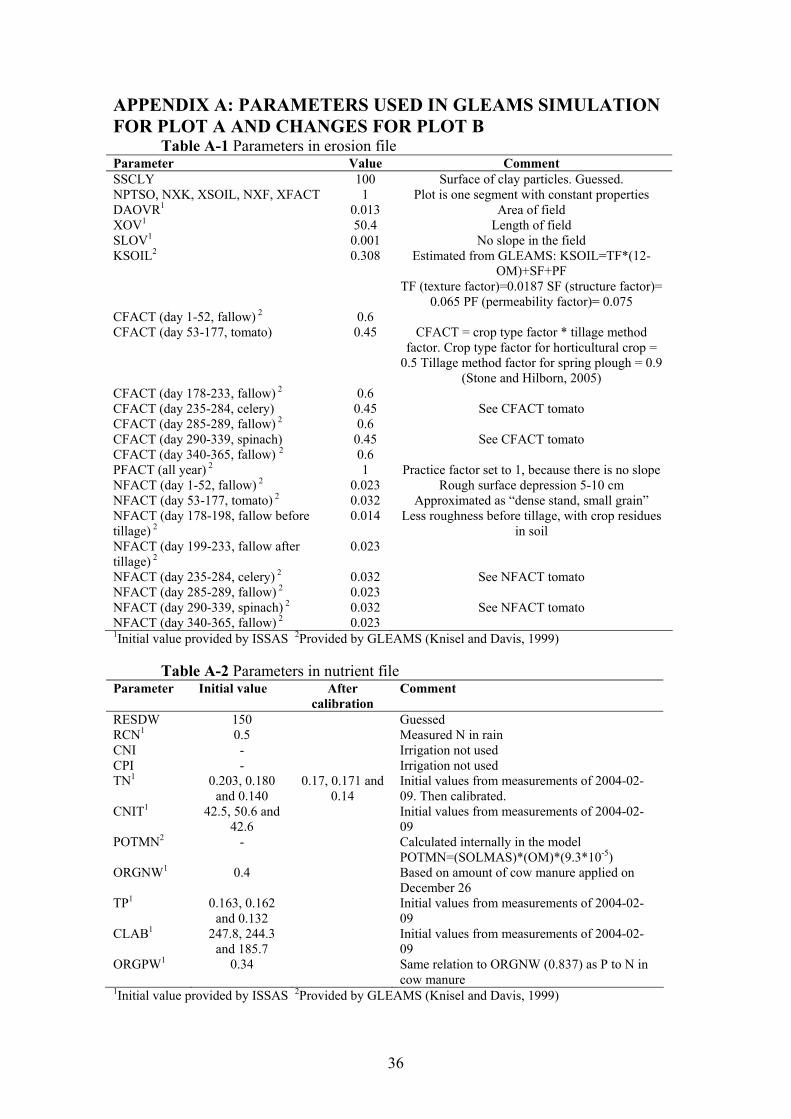
36

APPENDIX A: PARAMETERS USED IN GLEAMS SIMULATION FOR PLOT A AND CHANGES FOR PLOT B

Table A-1 Parameters in erosion file Parameter Value Comment SSCLY 100 Surface of clay particles. Guessed. NPTSO, NXK, XSOIL, NXF, XFACT 1 Plot is one segment with constant properties DAOVR1 0.013 Area of field XOV1 50.4 Length of field SLOV1 0.001 No slope in the field KSOIL2 0.308 Estimated from GLEAMS: KSOIL=TF*(12-

OM)+SF+PF TF (texture factor)=0.0187 SF (structure factor)=

0.065 PF (permeability factor)= 0.075 CFACT (day 1-52, fallow) 2 0.6 CFACT (day 53-177, tomato) 0.45 CFACT = crop type factor * tillage method

factor. Crop type factor for horticultural crop = 0.5 Tillage method factor for spring plough = 0.9

(Stone and Hilborn, 2005) CFACT (day 178-233, fallow) 2 0.6 CFACT (day 235-284, celery) 0.45 See CFACT tomato CFACT (day 285-289, fallow) 2 0.6 CFACT (day 290-339, spinach) 0.45 See CFACT tomato CFACT (day 340-365, fallow) 2 0.6 PFACT (all year) 2 1 Practice factor set to 1, because there is no slope NFACT (day 1-52, fallow) 2 0.023 Rough surface depression 5-10 cm NFACT (day 53-177, tomato) 2 0.032 Approximated as “dense stand, small grain” NFACT (day 178-198, fallow before tillage) 2

0.014 Less roughness before tillage, with crop residues in soil

NFACT (day 199-233, fallow after tillage) 2

0.023

NFACT (day 235-284, celery) 2 0.032 See NFACT tomato NFACT (day 285-289, fallow) 2 0.023 NFACT (day 290-339, spinach) 2 0.032 See NFACT tomato NFACT (day 340-365, fallow) 2 0.023 1Initial value provided by ISSAS 2Provided by GLEAMS (Knisel and Davis, 1999)

Table A-2 Parameters in nutrient file Parameter Initial value After

calibration Comment

RESDW 150 Guessed RCN1 0.5 Measured N in rain CNI - Irrigation not used CPI - Irrigation not used TN1 0.203, 0.180

and 0.140 0.17, 0.171 and

0.14 Initial values from measurements of 2004-02-09. Then calibrated.

CNIT1 42.5, 50.6 and 42.6

Initial values from measurements of 2004-02-09

POTMN2 - Calculated internally in the model POTMN=(SOLMAS)*(OM)*(9.3*10-5)

ORGNW1 0.4 Based on amount of cow manure applied on December 26

TP1 0.163, 0.162 and 0.132

Initial values from measurements of 2004-02-09

CLAB1 247.8, 244.3 and 185.7

Initial values from measurements of 2004-02-09

ORGPW1 0.34 Same relation to ORGNW (0.837) as P to N in cow manure

1Initial value provided by ISSAS 2Provided by GLEAMS (Knisel and Davis, 1999)

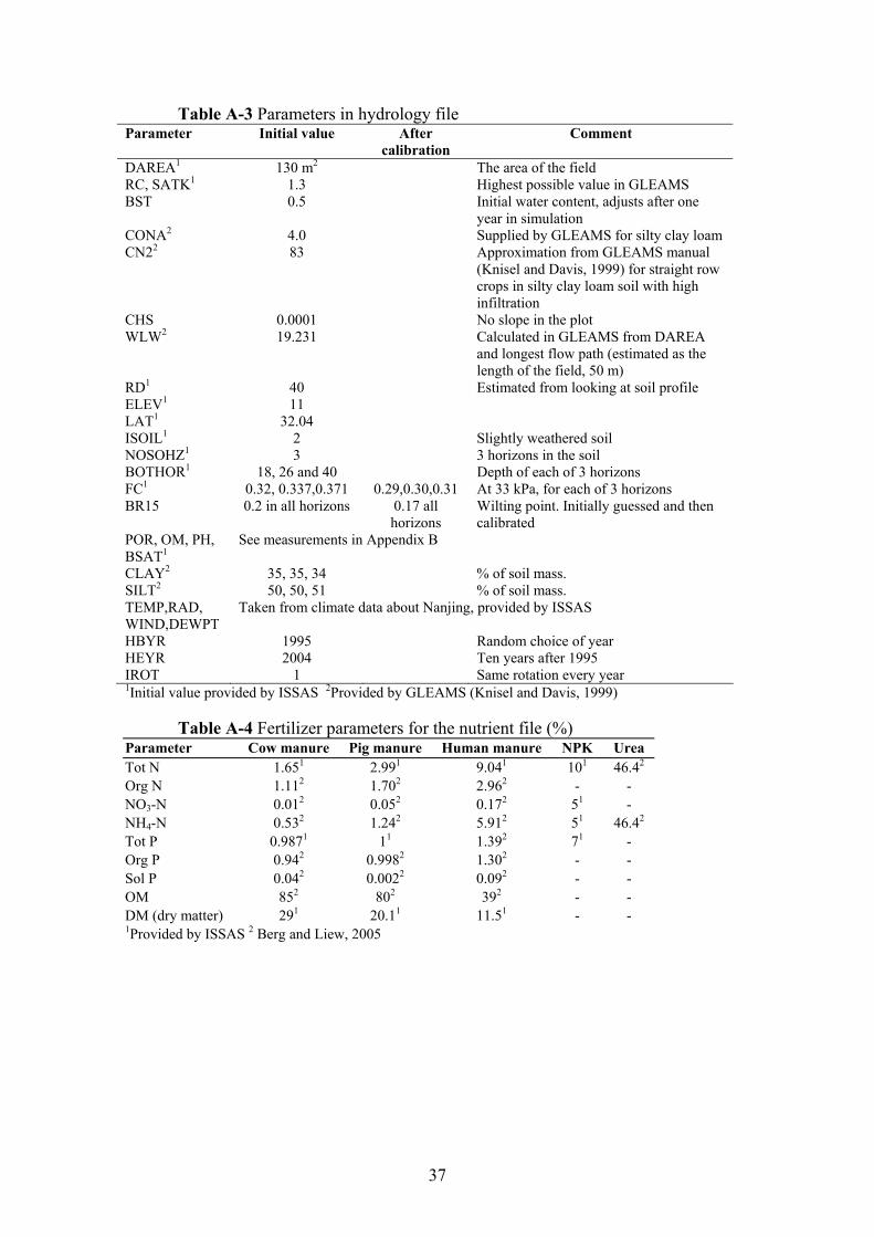
37

Table A-3 Parameters in hydrology file Parameter Initial value After

calibration Comment

DAREA1 130 m2 The area of the field RC, SATK1 1.3 Highest possible value in GLEAMS BST 0.5 Initial water content, adjusts after one

year in simulation CONA2 4.0 Supplied by GLEAMS for silty clay loam CN22 83 Approximation from GLEAMS manual

(Knisel and Davis, 1999) for straight row crops in silty clay loam soil with high infiltration

CHS 0.0001 No slope in the plot WLW2 19.231 Calculated in GLEAMS from DAREA

and longest flow path (estimated as the length of the field, 50 m)

RD1 40 Estimated from looking at soil profile ELEV1 11 LAT1 32.04 ISOIL1 2 Slightly weathered soil NOSOHZ1 3 3 horizons in the soil BOTHOR1 18, 26 and 40 Depth of each of 3 horizons FC1 0.32, 0.337,0.371 0.29,0.30,0.31 At 33 kPa, for each of 3 horizons BR15 0.2 in all horizons 0.17 all

horizons Wilting point. Initially guessed and then calibrated

POR, OM, PH, BSAT1

See measurements in Appendix B

CLAY2 35, 35, 34 % of soil mass. SILT2 50, 50, 51 % of soil mass. TEMP,RAD, WIND,DEWPT

Taken from climate data about Nanjing, provided by ISSAS

HBYR 1995 Random choice of year HEYR 2004 Ten years after 1995 IROT 1 Same rotation every year 1Initial value provided by ISSAS 2Provided by GLEAMS (Knisel and Davis, 1999)

Table A-4 Fertilizer parameters for the nutrient file (%) Parameter Cow manure Pig manure Human manure NPK Urea Tot N 1.651 2.991 9.041 101 46.42 Org N 1.112 1.702 2.962 - - NO3-N 0.012 0.052 0.172 51 - NH4-N 0.532 1.242 5.912 51 46.42 Tot P 0.9871 11 1.392 71 - Org P 0.942 0.9982 1.302 - - Sol P 0.042 0.0022 0.092 - - OM 852 802 392 - - DM (dry matter) 291 20.11 11.51 - - 1Provided by ISSAS 2 Berg and Liew, 2005

38

TableA-5 Crop and nutrient parameters Parameter Initial values After calibration Comment

Celery Spinach Tomato Celery Spinach Tomato

ICROP 82 84 85 Crop code to identify crop in model

LEG 0 0 0 Non-leguminous crops PY 40000 14900 77000 9000 Potential yield,

estimated by farmer DMY 1.5 1.35 1.45 CNR 40 40 40 C1 0.17 0.36 0.27 0.27 0.43 0.2 C2 -0.66 -0.494 -0.56 Root dpth (cm) 30 30 60

According to GLEAMS database3. Celery estimated as lettuce1

RNP 4.192 5.63 8.6 3.5

Relation of N to P. Celery analysed by ISSAS. Others from GLEAMS database3

Crop ht (m) 0.41 0.3 1 0.4 0.4 1.5 Celery measured in field. Others from GLEAMS database3

1Berg and Liew, 2005 2Provided by ISSAS 3Knisel and Davis (1999)

Table A-6 Parameters for application of fertilizer and tillage (provided by author) Parameter Value MFERT 0: NPK, Urea

1: Manure METHAP (Urea) 3 (Fertigation) MTYPE (Manure) 15 (Parameters user supplied) DEPIN (Manure and NPK) 0 for surface application.

10 cm for cow manure. FRWAT (Urea) 0.5 or 1 cm depending on amount of urea WASTYP 1 (solid): Cow and pig 2 (slurry): Human LTIL (tillage on July 17) 6 (Row cultivator) DTIL (tillage on July 17) 30 cm LTIL (incorporation of cow manure) 23 (Parameters user supplied) DTIL (incorporation of cow manure) 10 cm (Estimation of depth of digging) EFFINC 0.9 (High efficiency of incorporation) FMIX 0.05 (Low efficiency of mixing)

Table A-7 Parameters changed for simulation on Plot B (except for management events) Parameter Value for Plot B Initial N content in 0-18 cm (%) 0.17 PY, Potential yield, celery 23000 PY, spinach 12000 PY, tomato 40000

39

Appendix B. Soil measurements provided by ISSAS

Table B-1. Soil measurements

Table B-2. Measurements of N content in each horizon on Plot A

Total N kg/ha NH4-N kg/ha NO3-N kg/ha Soil depth, cm Date

0-18 18-26 26-40 0-18 18-26 26-40 0-18 18-26 26-40

2004-02-09 4745 1911 2967 292.0 119.0 95.6 99.4 53.7 90.1 2004-03-24 35.9 4.43 7.13 507 83.9 94.7 2004-05-14 14.9 4.72 5.44 494 99.1 131 2004-07-12 19.6 6.49 11.1 211 61.1 96.1 2004-09-30 4381 1852 2489 19.8 7.31 13.4 120 73.9 147 2004-11-9 4687 1802 2251 68.9 12.3 14.2 526 123 166

Table B-3. Measurements of soil water content in each horizon on Plot A(% of volume).1 Date 0-18 cm 18-26 cm 26-40 cm 2004-02-09 22.1 28.8 31.7 2004-03-24 25.1 29.4 30.8 2004-05-14 28.5 27.4 30.8 2004-07-12 22.7 23.7 27.3 2004-09-30 18.7 29.3 32.1 2004-11-9 24.9 27.3 29.7 1Data provided in cm water per weight, and then converted to % of volume by multiplying with bulk density.

Table B-4. Crop and fertilizer analysis for Plot A Crop/Fertilizer N (% of DM) P (% of DM) Dry matter (DM)(%) Tomato (edible+non-edible) 1.7 0.49 11 Celery 3.4 0.82 9 Spinach 4.9 0.74 9 Cow manure 1.65 0.987 29

Parameter Horizon 0-18 cm Horizon 18-26 cm Horizon 26-40 cm Saturated hydraulic conductivity (cm/h) 1.458 1.458 1.458

Porosity 50.9 50.2 42.6 Water holding capacity (volume %) 0.03 MPa 32.0 33.7 37.1

Bulk density 1.3 1.32 1.52 Clay (<0.002mm) content (% of volume) 46.28 47.66 45.46

Silt (0.002-0.05mm) content (% of volume) 46.31 46.32 49.38

Sand (>0.05mm) content (% of volume) 7.41 6.02 5.16

Organic matter content (% of volume) 3.38 2.44 1.23

Base saturation (%) 100 97.9 80.9

40

Appendix C. Long term N and P simulations of Plot A and Scenario

8 0 0 0

8 2 0 0

8 4 0 0

8 6 0 0

8 8 0 0

9 0 0 0

9 2 0 0

9 4 0 0

9 6 0 0

9 8 0 0

J a n -9 5 J a n -9 6 J a n -9 7 J a n -9 8 J a n -9 9 J a n -0 0 J a n -0 1 J a n -0 2 J a n -0 3 J a n -0 4 Figure C-1 Simulated total N content over 10 years on Plot A.

0

20 00

40 00

60 00

80 00

1 00 00

1 20 00

J an -95 Ja n -96 Ja n -9 7 J an -98 J an -99 Ja n -0 0 J a n -0 1 J an -02 J an -03 J an -04

Figure C-2 Simulated total P content over 10 years on Plot A.

830084008500860087008800890090009100920093009400

Jan-95 Jan-96 Jan-97 Jan-98 Jan-99 Jan -00 Jan -01 Jan -02 Jan -03 Jan -04

Figure C-3 Simulated total N content over 10 years for the scenario on Plot A.

0

2000

4000

6000

8000

10000

12000

Jan-95 Jan-96 Jan-97 Jan-98 Jan-99 Jan-00 Jan-01 Jan-02 Jan-03 Jan-04

Figure C-4. Simulated total P content over 10 years for the scenario on Plot A

41

APPENDIX D: THE EFFECT OF WILTING POINT ON DECOMPOSITION OF MANURE

0

100

200

300

400

500

600

700

Dec-96Jan-97

Feb-97Mar-97

Apr-97May-97

Jun-97Jul-97

Aug-97Sep-97

Oct-97Nov-97

Nitr

ogen

in a

pplie

d m

anur

e (k

g ha

-1)

WP = 0.2

WP = 0.17

Figure D-1 The pattern of decomposition of manure applied on December 26 on Plot A for two different wilting points