Embed Size (px)
Citation preview
Modelling impacts of climate change on water resources in the Volta
Basin, West Africa
Dissertation
zur
Erlangung des Doktorgrades (Dr. rer. nat)
der
Mathematisch-Naturwissenschaftlichen Fakultät
der
Rheinischen Friedrich-Wilhelms-Universität Bonn
vorgelegt von
RAYMOND ABUDU KASEI
aus
TAMALE; GHANA
Bonn 2009

1. Referent: Prof. Dr. Bernd Diekkrüger 2. Referent: Prof. Dr. Paul Vlek Tag der Promotion: 11.12.2009 Erscheinungsjahr: 2010 Diese Dissertation ist auf dem Hochschulschriftenserver der ULB Bonn http://hss.ulb.uni-bonn.de/diss_online elektronisch publiziert
ABSTRACT
The Volta River Basin is one of the largest river systems in Africa covering an area of approximately 400,000 km2 and shared by six riparian states of West Africa. The semi-arid to sub-humid regions of the basin are climate sensitive. The population is mainly dependent on rainfed agriculture and therefore highly vulnerable to the spatial and temporal variability to rainfall and climate change. Even though the per capita water availability of the basin may be perceived as normal, deforestation, land degradation, and high population growth rate coupled with global climate change promises to exacerbate the growing scarcity on water resources due to climate change, as water supplies are unreliable and insufficient to meet the water demands of the growing population. The basin has experienced prolonged dry seasons when many rivers and streams dried up, and lately flooding due to excessive rainfall.
To assess the impact of plausible global climate change to regional climate as well as land surface and as to sub-surface hydrology in the region of the Volta Basin, hydrology simulations were performed with the use of calibrated regional climate models.
The WaSiM-ETH hydrological model was calibrated and validated at Pwalugu (north of basin) and Bui (south of basin). Using the WaSiM-simulated water balance for the period 1961-2000 as the basis for comparison, the simulated future (2001-2050) water balance in the Volta Basin shows increases in the mean annual discharge and surface runoff with the regional model MM5 and decreases with the regional model REMO.
The results of the MM5 and WaSiM simulations show an annual mean temperature increase of 1.2 oC over the basin. Mean annual precipitation increases for both the north and the south of the basin are projected. The averaged increase over the basin is about 15 %. The simulated mean change in discharge at the subsurface is about 40 % of total rainfall between the periods 1991-2000 and 2030-2039. Consequently, interflow and base flows are expected to increase in the range of 0 and 20 %, respectively.
The results of two ensemble runs of the IPCC scenarios A1B and B1 by REMO applied to WaSiM show an annual mean increase in temperature of 1oC. Precipitation over the basin is expected to reduce between 3 % and 6 % in the period 2001-2050 compared to 1961-2000. An average decrease of 5 % is projected for total discharge with corresponding decreases in surface, lateral and base flows.
KURZFASSUNG
Modellierung der Auswirkung des Klimawandels auf die Wasserressourcen des Volta Einzugsgebiet, Westafrika Das Voltabecken ist eines der größten Flusssysteme in Afrika und erstreckt sich über eine Fläche von circa 400.000 km2 mit sechs westafrikanischen Anrainerstaaten. Die semi-ariden bis sub-humiden Regionen desVoltaeinzugsgebieest gehören zu den klimasensitiven Gebieten Afrikas. Die Bevölkerung ist überwiegend vom Regenfeldbau abhängig und daher sehr stark durch die räumliche und zeitliche Variabilität von Niederschlag und deren Änderung aufgrund des Klimawandels beeinflusst.
Obwohl die mittlere Wasserverfügbarkeit pro Kopf der Bevölkerung im Einzugsgebiet nicht auf einen hohen Wasserstress hinweist, gibt es einen großen Gradienten zwischen dem Süden Ghanas und dem Norden Burkina Fasos. Es ist zu erwarten, dass Abholzung, Landdegradation und ein hohes Bevölkerungswachstum zusammen mit dem globalen Klimawandel zu einer Abnahme der verfügbaren Wasserressourcen führen wird, so dass der Wasserbedarf der zunehmenden Bevölkerung nicht befriedigt werden kann.
In der Vergangenheit gab es im Einzugsgebiet einerseits lange Trockenzeiten, in denen Flüsse und Bäche austrockneten, sowie andererseits, wie in den letzten Jahren, extreme Überschwemmungen aufgrund von sehr starken Niederschlägen. Es ist zu erwarten, dass sich diese Extreme verstärken werden.
Um die Auswirkungen des zu erwartenden globalen Klimawandels auf das regionale Klima und die Landoberfläche sowie auf die Wasserressourcen des Voltabeckens zu quantifizieren, wurden hydrologische Simulationen durchgeführt. Dafür wurde das hydrologische Modell WaSiM-ETH anhand der Abflüsse in Pwalugu (im Norden des Einzugsgebietes) und Bui (im Süden des Einzugsgebietes) kalibriert und validiert. Mit dem kalibrierten Modell wurden verschiedene Klimaszenarien berechnet, die mit zwei regionalen Klimamodellen erzeugt wurden.
Die Klimaszenarien des MM5 Modells zeigen eine Zunahme der Niederschläge für den Zeitraum 2030-2039 was zu einer Zunahme der Wasserverfügbarkeit und der Abflüsse führt. Im Gegensatz dazu berechnet das Modell REMO für den Zeitraum 2001-2050 eine Abnahme der Niederschläge und somit eine Abnahme des verfügbaren Wassers.
Die Ergebnisse der MM5-WaSiM-Simulationen zeigen eine jährliche mittlere Temperaturzunahme von 1,2 oC und eine Zunahme des Niederschlags sowohl im Norden als auch im Süden des Einzugsgebietes von ca. 15 %. Die simulierte mittlere Zunahme des Gesamtabflusses beträgt ca. 40 % für den Zeitraum 2030-2039 verglichen mit 1991-2000. Als Folge der Änderung im Niederschlag wird eine Zunahme des Zwischenabflusses und des Basisabflusses von 0 bis 20 % erwartet.
Die REMO-WASIM Ergebnisse der Ensembleläufe der beiden IPCC-Szenarien A1B und B1 zeigen eine jährliche mittlere Temperaturzunahme von 1oC. Die Niederschläge nehmen zwischen 3 % und 6 % im Zeitraum 2001-2050 im Vergleich zum Zeitraum 1961-2000 ab. Eine durchschnittliche Abnahme des Gesamtabflusses von 5 % wird durch entsprechende Abnahmen des Oberflächen-, Zwischen- und Basisabflusses erfolgen.
TABLE OF CONTENTS
1 GENERAL INTRODUCTION ----------------------------------------------------- 1
1.1 Introduction ---------------------------------------------------------------------------- 1 1.2 Motivation ----------------------------------------------------------------------------- 4 1.3 Objectives ------------------------------------------------------------------------------ 6 1.4 Questions ------------------------------------------------------------------------------- 6 1.5 Thesis structure ------------------------------------------------------------------------ 6
2 STUDY AREA ------------------------------------------------------------------------ 8
2.1 Location and overview --------------------------------------------------------------- 8 2.1.1 White Volta Basin ------------------------------------------------------------------ 11 2.1.2 Black Volta Basin ------------------------------------------------------------------- 12 2.1.3 Lower Volta Basin ------------------------------------------------------------------ 13 2.1.4 Oti Basin ----------------------------------------------------------------------------- 14 2.2 Vegetation ---------------------------------------------------------------------------- 14 2.3 Climate ------------------------------------------------------------------------------- 15 2.3.1 Temperature ------------------------------------------------------------------------- 15 2.3.2 Precipitation ------------------------------------------------------------------------- 16 2.3.3 Evaporation -------------------------------------------------------------------------- 18 2.4 Geology and soils ------------------------------------------------------------------- 19 2.5 Land use and agriculture ----------------------------------------------------------- 22 2.6 Hydrology and water resources --------------------------------------------------- 22
3 CLIMATOLOGICAL AND HYDROLOGICAL DATA --------------------- 24
3.1 Data availability --------------------------------------------------------------------- 24 3.1.1 Data quality assessment ------------------------------------------------------------ 25 3.2 Climate data ------------------------------------------------------------------------- 26 3.2.1 Meteorological agencies ----------------------------------------------------------- 27 3.2.2 GLOWA Volta Project (GVP) ---------------------------------------------------- 29 3.3 Hydrological data ------------------------------------------------------------------- 30 3.3.1 Hydrological Service Department ------------------------------------------------ 31 3.3.2 GLOWA Volta Project ------------------------------------------------------------- 34
4 METHODOLOGY ----------------------------------------------------------------- 35
4.1 Model selection --------------------------------------------------------------------- 36 4.2 Basic concept ------------------------------------------------------------------------ 37 4.3 Running WaSiM-ETH for the Volta Basin -------------------------------------- 38 4.4 Model construction ----------------------------------------------------------------- 40 4.5 Calibration and validation --------------------------------------------------------- 41 4.6 Predictive validity ------------------------------------------------------------------- 44 4.6.1 Pearson’s r and R2------------------------------------------------------------------- 44 4.6.2 Nash-Sutcliffe efficiency index --------------------------------------------------- 45
4.6.3 Index of Agreement (d) ------------------------------------------------------------ 46 4.6.4 Mass balance error ------------------------------------------------------------------ 46 4.7 Drought analysis in the Volta Basin ---------------------------------------------- 46 4.8 Historical drought events in the Volts Basin ------------------------------------ 48 4.9 Regional drought analysis --------------------------------------------------------- 49
5 HYDROLOGICAL MODEL WASIM-ETH ------------------------------------ 51
5.1 Introduction -------------------------------------------------------------------------- 51 5.2 WaSiM Concept --------------------------------------------------------------------- 51 5.3 Data requirements and processing in WaSiM ----------------------------------- 52 5.3.1 Temporal data ----------------------------------------------------------------------- 52 5.3.2 Spatial data --------------------------------------------------------------------------- 53 5.4 WASIM-ETH modules ------------------------------------------------------------- 57 5.4.1 Potential and real evapotranspiration --------------------------------------------- 57 5.4.2 Interception -------------------------------------------------------------------------- 58 5.4.3 Snow module ------------------------------------------------------------------------ 59 5.4.4 Infiltration and the unsaturated zone module ------------------------------------ 59 5.4.5 Run-off routing ---------------------------------------------------------------------- 61 5.4.6 Reservoir ----------------------------------------------------------------------------- 62 5.5 Calibration of WaSiM-ETH ------------------------------------------------------- 63 5.6 Main calibration parameters ------------------------------------------------------- 63 5.7 Calibration results ------------------------------------------------------------------- 65 5.8 Model performance ----------------------------------------------------------------- 70 5.9 Validation results ------------------------------------------------------------------- 72 5.10 Water Balance ----------------------------------------------------------------------- 74
6 DROUGHT IN THE VOLTABASIN -------------------------------------------- 77
6.1 Introduction -------------------------------------------------------------------------- 77 6.2 Regional climate trends and global climate change ---------------------------- 78 6.3 Drought in the Volta basin --------------------------------------------------------- 79 6.4 Rainfall anomalies in the Volta Basin -------------------------------------------- 80 6.5 Standardized precipitation index (SPI) ------------------------------------------- 82 6.6 Rainfall anomalies and impacts --------------------------------------------------- 84
7 CHANGES IN HYDROLOGY AND RISKS FOR WATER
RESOURCES IN THE VOLTA BASIN ---------------------------------------- 91
7.1 Introduction -------------------------------------------------------------------------- 91 7.2 Climate change ---------------------------------------------------------------------- 93 7.3 Regional climate scenarios – MM5 ----------------------------------------------- 94 7.3.1 Highlights of MM5 on the Volta Basin ------------------------------------------ 95 7.4 Regional climate scenarios – REMO -------------------------------------------- 102 7.4.1 Highlights of REMO on Volta Basin area -------------------------------------- 104 7.5 Regional climate model performance of MM5 and REMO ------------------ 106 7.6 Comparison of past, present and future hydrological dynamics of the
Volta Basin ------------------------------------------------------------------------- 110
7.7 Future projections ------------------------------------------------------------------ 111 7.8 Water balance dynamics ---------------------------------------------------------- 111 7.9 Soil moisture ------------------------------------------------------------------------ 117 7.10 Risk for water resources ----------------------------------------------------------- 118 7.11 Impacts of climate change on Volta Basin water resources ------------------ 123 7.12 Comparison of study results with previous studies ---------------------------- 124
8 CONCLUSIONS AND OUTLOOK -------------------------------------------- 126
8.1 Conclusions ------------------------------------------------------------------------- 126 8.2 Outlook ------------------------------------------------------------------------------ 128
9 REFERENCES --------------------------------------------------------------------- 130
10 APPENDIX ------------------------------------------------------------------------ 141

List of Abbreviations
AGCMs Atmospheric global circulation models
AMO Atlantic Multidecadal Oscillation
CRU Climate Research Unit
CV Correlation Variance
DEM Digital Elevation Model
ENSO El Nino Southern Oscillation
ET Evapotranspiration
ETP Potential Evapotranspiration
FAO Food and Agriculture Organization
FDCs Frequency Distribution Curves
GDP Gross Domestic Product
GHG Green House Gas
GMA Ghana Meteorological Agency
HSD Hydrological Services Department
HSPF Hydrologic Simulation Program FORTRAN
IDW Inverse Distance Weighting
IIED International Institute of Environment and Development
IPCC Intergovernmental Panel on Climate Change
ITCZ Inter-Tropical Convergence Zone
IUCN International Union for Conservation of Nature
LAI Leaf Area Index
MM5 Meteorological Model version 5
MOS model output statistics
MPI Max-Planck-Institute for Meteorology
NCAR National Center for Atmospheric Research
PMCC Pearson product-moment correlation coefficient
PSU Pennsylvania State University
RCMs Regional Climate Models
SHE Hydrological system model
SPI Standardized Precipitation Index
SRTM Shuttle Radar Topography Mission

SSTs Sea Surface Temperatures
UNFCCC United Nations Convention on Climate Change
WaSiM-ETH Water Balance Simulation model –ETH
WPI Water Poverty Index

General introduction
______________________________________________________________________
1
1 GENERAL INTRODUCTION
1.1 Introduction
While still debated amongst politicians and economists, most of the natural science
community agrees that global warming is occurring as a result of anthropogenic
activities and is causing climate change. The United Nations Convention on Climate
Change (UNFCCC) is the foremost governmental body with global authority and the
intent to understand and address the effects of global warming. The UNFCCC addresses
climate change in terms of two basic premises: mitigation, reducing the causes of
anthropogenic activities on the natural environment, and adaptation, preparing for the
effects of a changed environment on human beings. The UNFCCC has observed that
those who are least responsible for climate change are also the most vulnerable to its
projected impacts. In no place is this more evident than in Sub-Saharan Africa, where
greenhouse gas (GHG) emissions are negligible. It is also important to note however
that considering the landcover changes mostly due to deforestation, GHG emissions of
sub-Sahara Africa may not be negligible. Extreme climate variability is expected to
impact on the inhabitants significantly. Interestingly, due to the sheer scale of African
sub-climates, the effects are also being perceived in terms of global dimensions, one
example being the relationship of the western winds from the Sahara desert and
hurricanes impacting the United States’ eastern seaboard. Such elements as changes in
vegetation, hydrology and dust export from land surface to atmosphere also have the
potential to modify large-scale atmospheric properties regionally and globally
(CLIVAR, 2004). In the not too far past, adaptation issues have largely been
overlooked, partly because the United Nations has focused its attention on the reduction
of GHG emissions and enhancing “ carbon sink” options. It is now evident that
irrespective of the measures and policies aimed at mitigating the impacts of climate
change there is an urgent need to build adaptive capacity to reduce vulnerability to
climate variability and change. Only recently the UNFCCC has begun to address
adaptation issues more directly through conferences and meetings of the involved
parties.
The Intergovernmental Panel on Climate Change (IPCC) has defined
adaptation as the “adjustment in natural or human systems in response to actual or
General introduction
______________________________________________________________________
2
expected climatic stimuli or their effects, in order to moderate harm.” While mitigation
represents activities to protect nature from society, in contrast, Stehr and Storch (2005)
describe adaptation to constitute ways of protecting society from nature. Adaptation has
always been an activity African societies have developed to prepare for changing
climatic conditions (Diamond, 2005); At present however, due to the global scale of
climate change causal relationships, locally derived knowledge, either intuitive or
historical, is often rendered irrelevant. It is this lack of ability for societal adjustment to
occur within a given timeframe that determines the magnitude of impacts as well as
their secondary consequences (Adger et al. 2004). Adaptation can be either reactive or
anticipatory according to UNEP (2008). UNEP found that in integrating adaptation to
climate change, usually happens only after initial impacts of climate change have
become manifest, then reactive adaptation occurs thereafter; whereas in anticipatory or
proactive approaches, adaptation takes place before the impacts are evident. The latter
type of adaptation is best seen as a process entailing more than merely the
implementation of a policy or the application of a technology. It is essentially a multi-
stage and reiterative process, involving four basic steps: 1) information development
and awareness raising, 2) planning and design, 3) implementation, and 4) monitoring
and evaluation. Inherently linked to the causes of global warming and climate change
are rapid population increases. Most African nations are witnessing exponential
population increases. As populations increase, government structures subdivide and
delegate authority to address local needs. The decentralization of government structures
presents opportunities and challenges to the development of adaptation frameworks.
With local governments taking on new and increasingly important roles, advantages are
presented, but these added benefits require more intergovernmental coordination and
cooperation as well as stakeholder engagement and consensus building.
The African continent is a vast land, and known to experience a wide variety
of climate regimes with varied magnitudes. Within the chapter on impacts, adaptation
and vulnerability in Africa the IPCC report on climate change (2001) states that
location, size, and shape of this continent play key roles in determining changes in
climate that is being observed. The pole-ward extremes of the continent example South
Africa are known to experience winter rainfall that are said to be associated with the
passage of mid-latitude air masses.
General introduction
______________________________________________________________________
3
According to the IPCC report on Climate Change (2001), precipitation has been
inhibited due to subsidence in areas like Kalahari and Sahara deserts almost throughout
the year. In equatorial and tropical areas however, moderate to heavy precipitation
known to be associated with the Inter-Tropical Convergence Zone (ITCZ) is
experienced. The position of maximum surface heating is at the equator which is linked
with meridional displacement of the overhead cast of the sun causes the movement of
the ITCZ, resulting in these parts to experience two rain seasons. Only one rainy season
is observed in areas further from the equatorial regions towards the poles (IPCC, 2001).
Semazzi and Sun (1995) found that the mean climate of the continent is further
modified by the presence of large distinctions in topography and the existence of large
lakes in many parts of the continent. Significantly, climatic variations and the persistent
decline in rainfall have been evident in most parts of Africa especially in the Sahel since
the late 1960s. In 1994, the West African Sahel experienced one of the wettest years
since the early 1960s as reported in LeCompte et al. (1994); and Nicholson et al. (1996).
With excess late rains of 1994 came some optimism that the dry conditions, which had
prevailed for nearly three decades, had finally ended. However, rainfall barely exceeded
the long-term mean. The observed persistent drying trend will ultimately result in loss
of water resources, losses in food production, displacement of people and a major
constraints on hydropower generation. These concerns are shared by governments and
development planners across African continent. The interannual variability of rainfall
over Africa, especially sub-Sahara, has been extensively analyzed by various authors in
numerous publications (e.g., Nicholson, 1979, 1983, 1985, 1993, 1994; Nicholson and
Palao, 1993; Nicholson et al. 1996; Nicholson et al. 2007) emphasizing the need to
address the rapid loss in water resources in the changing climate.
The Volta basin, which is the major focus of this research, generates the major
surface and ground water resources for the riparian countries Ghana, Burkina Faso and
Togo. Analyses of rainfall data from various stations within the Volta River system
indicate that the months in which precipitation exceeds the evapotranspiration to
generate runoff and direct recharge are usually June, July, August, and September.
Martin (2005) found out that the annual recharge for the Volta River system ranges
from 13 % to 16 % of the mean annual precipitation.
General introduction
______________________________________________________________________
4
Throughout the Volta Basin, reservoirs and dams have been constructed to mobilize
water for agricultural, hydro-electricity generation and industrial use. The number of
large and small dams continues to increase in line with increasing settlements and
increasing population growth.
Van Edig et al. (2001) state that, major conflict potential exists between the
two main users of the basin; Ghana and Burkina Faso. Ghana is known to rely heavily
on the flow of the Volta primarily for hydro-power whose water heads originate in
Burkina Faso. Burkina Faso on the other hand, dam most of its tributaries for the
purposes of irrigated agriculture. The tension arises from Ghana wanting Burkina Faso
to keep the water flowing. In recent decades, most especially from the severe droughts
that hit the region from the 1980s, the fresh water needs and demands of Burkina Faso
have increased, thus pushing the country to increase the number of dams in the Volta
River Basin to meet the growing demand. This has further compounded the already
tensed relation with Ghana. Impacts of climate change with the anticipated increase
in potential evaporation and a reduction in precipitation threaten to exacerbate the
problems related to lack of adequate water resources in the basin.
1.2 Motivation
Water and food are becoming the critical factors after wars in the development of the
sub-humid and semi-arid countries of West Africa. Millions of people in the developing
countries die every year of water-related diseases. Modern developments, changing life
styles and population growth have greatly increased water demand. As water crises are
forecasted for the future, and meeting the water demands of the increasing population in
the Volta basin is closely tied to understanding and the development of groundwater,
surface and coastal water resources in order to prevent their depletion. The Regional
model REMO, a climatic model downscaled from Global models was applied by the
GLOWA Impetus project to access the changes in climate for part of the region.
Until the year 2050, Paeth et al. (2007) project a decrease in rainfall of around
25-30 %, which is comparable to the observed decline after the 1960s. Other regional
climate simulations for the Volta Basin predict an overall slight increase of the total
yearly rainfall, exhibiting strong spatial (-20 % to + 50 %) and temporal heterogeneity (-
20 % to +20 %) (Kunstmann and Jung, 2005). Over the last decade, a number of
General introduction
______________________________________________________________________
5
climatic models have conflicting predictions over the sign of the variation for the
continent of Africa and especially at large regional scales such as for West Africa.
Although individual models may disagree on the signs, but there is a consensus on the
increase of the frequency of extreme events for the future (Hewitson, and Crane (2006),
IPCC-AR4 (2005)).
Water resources systems in the Volta Basin are very sensitive to climatic
variations. During the 1980s and 1990s, there were several drought events that affected
water resources (International Institute of Environment and Development - IIED, 1992),
exacerbated by an enhanced hydrologic seasonality. The aggravation of seasonal rainfall
coupled with a changing climate may have profound effects on water resources systems
in areas that are known to be already vulnerable, such as the northern part of the Volta
Basin. The geology of many areas results in a low groundwater storage potential and
groundwater recharge, resulting in an over reliance on surface water resources. These
resources are depleted rapidly during a dry period in most areas and water quality is
decreasing with decreased quantity.
The rapid growth of about 3 % per annum in the basin’s population will put
constraints on the quantity and quality of water with time. Climate change may put
further constraints on the water resources because of changes in spatial and temporal
distribution of the resources which several studies such as the Green Cross International
report (2001) have shown that unless proactive measures are employed the resources
will not be able to stand-up to such constraints. Therefore, there is a need to modify or
design methods and/or programs to evaluate risk and uncertainty under the present
understood climate-generating mechanisms. This is critical in evaluating future risks of
droughts, floods, threats to food security, and the reliability of hydropower generation.
Until very recently, there was little or no hydro-meteorological information on
the Volta Basin of West Africa contributing to the challenges faced in sustainable
water-management programmes (FAO, 2005). This drives the core of the objectives of
this research, which are to determine if a mainly model-based water balance monitoring
system can be used to provide a scientific and reliable quantification of the spatial and
temporal changes of water fluxes in the Volta catchment for predicting extreme events
such as droughts. This information is of immense importance for decision and policy
makers in water resources management in the Volta Basin.
General introduction
______________________________________________________________________
6
1.3 Objectives
1. Assess changes in precipitation and runoff over the recent past using historical
meteorological and hydrological data.
2. Assess the impact of projected climate change using MM5 and REMO climate
inputs on surface runoff of the Volta Basin.
1.4 Questions
How can we characterize statistically the variations in climate or weather within
the Volta Basin over the recent historical period?
Are model-generated simulations of climate and hydrologic conditions capable of
depicting such variation realistically? How can the probabilities of adverse
climate events (droughts) and associated water scarcity be modeled?
What risks apply to water availability and modeled soil moisture for improving
farming in the Volta Basin
1.5 Thesis structure
This thesis is organized in eight chapters. The first chapter gives a general introduction
to climate and the changes that have been observed within the region in various studies.
This includes objectives and research questions that this research seeks to answer. The
Volta Basin is described in relation to noticeable climate variability in Chapter 2.
Climate and hydrological data availability and data quality assessments are discussed in
Chapter 3; Chapter 4 describes the methodology used for this research. Chapters 5
through 7 focuses on the Water Balance Simulation model WaSiM-ETH model (Jasper
and Schulla, 1999) and some of the results obtained from the modules which are the
independent processes on which the WaSiM model runs. Chapter 5 concentrates on
concepts of WaSiM-ETH and the adaptation of the model to the study site. This
involves the calibration, validation and predictive analysis of the model. Chapter 6,
which is one of the major results chapters, seeks to assess drought occurrences against
precipitation and stream flow at selected stations within the catchments. From the 40
year simulation beginning 1961, Chapter 7, a key synthesis chapter, discusses the
changing hydrological time series of the Volta basin and accompanying risk for water
resources with emphasis on future prediction by a regional downscaled climatic model-

General introduction
______________________________________________________________________
7
MM5 done by Jung (2006) and REMO by Paeth (2005). The key results are
summarized and discussed in Chapter 8, which includes the general conclusions and
recommendations.
Study area
______________________________________________________________________
8
2 STUDY AREA
2.1 Location and overview
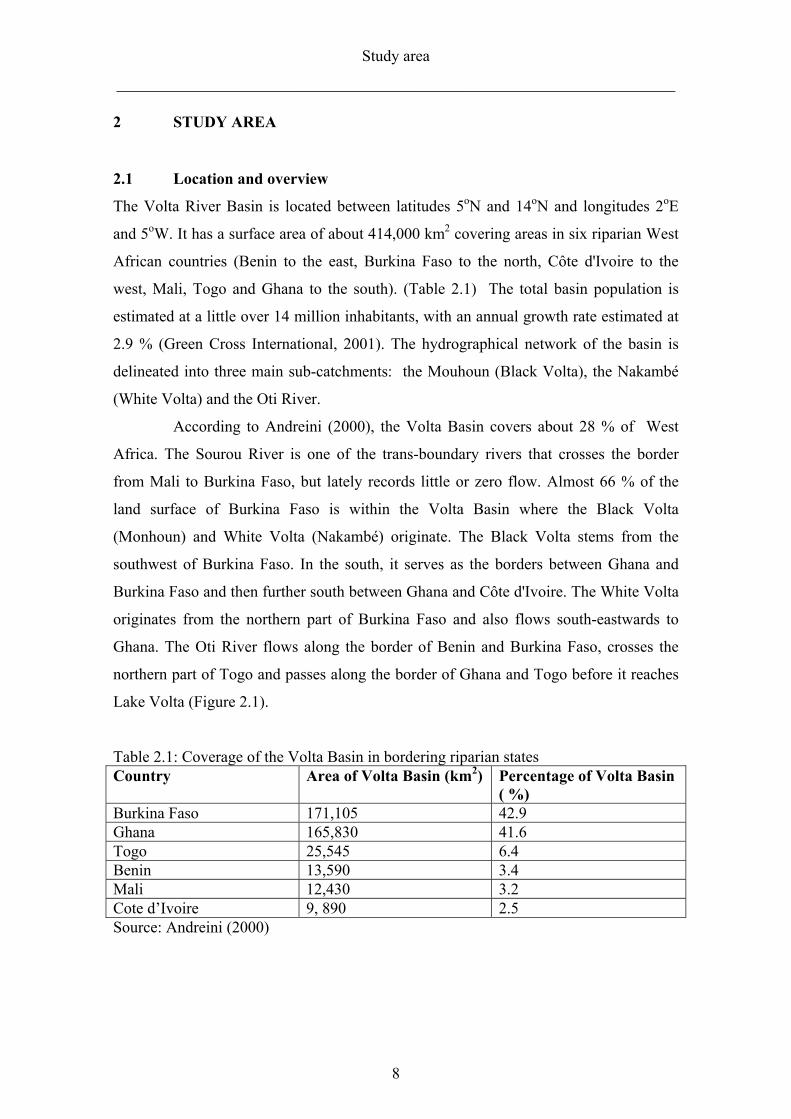
The Volta River Basin is located between latitudes 5oN and 14oN and longitudes 2oE
and 5oW. It has a surface area of about 414,000 km2 covering areas in six riparian West
African countries (Benin to the east, Burkina Faso to the north, Côte d'Ivoire to the
west, Mali, Togo and Ghana to the south). (Table 2.1) The total basin population is
estimated at a little over 14 million inhabitants, with an annual growth rate estimated at
2.9 % (Green Cross International, 2001). The hydrographical network of the basin is
delineated into three main sub-catchments: the Mouhoun (Black Volta), the Nakambé
(White Volta) and the Oti River.
According to Andreini (2000), the Volta Basin covers about 28 % of West
Africa. The Sourou River is one of the trans-boundary rivers that crosses the border
from Mali to Burkina Faso, but lately records little or zero flow. Almost 66 % of the
land surface of Burkina Faso is within the Volta Basin where the Black Volta
(Monhoun) and White Volta (Nakambé) originate. The Black Volta stems from the
southwest of Burkina Faso. In the south, it serves as the borders between Ghana and
Burkina Faso and then further south between Ghana and Côte d'Ivoire. The White Volta
originates from the northern part of Burkina Faso and also flows south-eastwards to
Ghana. The Oti River flows along the border of Benin and Burkina Faso, crosses the
northern part of Togo and passes along the border of Ghana and Togo before it reaches
Lake Volta (Figure 2.1).
Table 2.1: Coverage of the Volta Basin in bordering riparian states Country Area of Volta Basin (km2) Percentage of Volta Basin
( %) Burkina Faso 171,105 42.9 Ghana 165,830 41.6 Togo 25,545 6.4 Benin 13,590 3.4 Mali 12,430 3.2 Cote d’Ivoire 9, 890 2.5 Source: Andreini (2000)

Study area
______________________________________________________________________
9
Table 2.2: Major river system of the Volta Basin
Source: Barry et al. (2005)
Volta Basin System Area (km2)
Black Volta 149,015
White Volta 104,752
Oti River 72,778
Lower Volta 62,651
Total 389,196
Study area
______________________________________________________________________
10
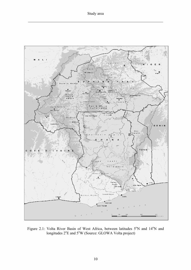
Figure 2.1: Volta River Basin of West Africa, between latitudes 5oN and 14oN and
longitudes 2oE and 5oW (Source: GLOWA Volta project)
Study area
______________________________________________________________________
11
Many other small tributaries have their source within Ghana, especially in the northern
savannah, but are dry after the rainy seasons. The groundwater in most parts of the basin
yield is little and cannot be depended on for extensive irrigation. In Akosombo to the
south of Ghana a dam was constructed for hydroelectric power. Behind this dam is one
of the world's largest artificial lakes,the Volta Lake, with a surface area of 8.500 km2
and a capacity of 148 km3. According to Andreini (2000), significant run-off occurs
only when the basin has received about 340 km3 of rainfall, and once this threshold is
reached, about 50 % of the total precipitation thereafter is as run-off. This implies
that small changes in rainfall could dramatically affect run-off rates. It is noted that,
although rainfall decreased by only 5 % from 1936 to 1998, run-off decreased by 14 %.
The average discharge flowing into the sea from this lake per annum is estimated at
about 38 km3.
2.1.1 White Volta Basin
The White Volta Basin, the second largest catchment of the Volta Basin, covers about
104,752 km2 and represents 46 % of the total Volta catchment area. It is located
within the Interior Savannah Ecological Zone and is underlaid by the Voltarian and
granite geologic formations (Opoku-Ankomah, 1998).
The main tributaries of the White Volta are the Morago and Tamne rivers.
The total surface area of the Morago is 1,608 km2 with 596 km2 in Ghana, 912 km2 in
Togo and 100 km2 in Burkina Faso. The Tamne tributary, however, lies entirely in
Ghana with a total area of 855 km2. The White Volta covers mainly the north-central
parts of Ghana (Barry et al., 2005).
Annual rainfall in this sub-basin (Opoku-Ankomah, 1998) ranges between
685 mm in the north (Mali) and 1,300 mm in the south (Ghana). Pan evaporation is
estimated to range between 1,400 mm to 3000 mm per annum with an average rainfall
runoff about 96.5 mm. The average annual runoff from the White Volta catchment is
estimated at 272m3/s. Barry et al. (2005) found a maximum annual flow of 1,216 m3/s
runoff at the peak of the rainy season and a minimum of about 0.11m3/s during the dry
season. Potential sites have been identified for storage within the basin totaling
nearly 8,180 x 106 m3 found to be capable of regulating the basin yield at a minimum
flow of about 209m3/s. The total annual flow contribution to the Volta Lake is about
Study area
______________________________________________________________________
12
20 %. Current surface water uses in the basin are estimated at about 0.11m3/s for
domestic and about 2m3/s for many small irrigation projects in the watersheds (Barry
et al., 2005). The construction of the Bagre dam covering a total area of 33,120 km2 in
1993 has changed the flow of the White Volta significantly, most especially the stable
base flow during the years. The annual average flow from the dam within the last
decade is estimated at 29.7m3/s. At the bottom and of the White Volta, an annual mean
discharge of 1,180 m3/s is observed at Akosombo (Rodier, 1964).
2.1.2 Black Volta Basin
The Black Volta Basin, the largest of the catchments in the Volta Basin has a total
area of 142,056 km2 of which 33,302 km2 (23.5 %) is located in Ghana. The
tributaries are the Aruba, Bekpong, Benchi, Chridi, Chuco Gbalon, Kamba, Kule
Dagare, Kuon, Laboni, Oyoko, Pale, and rivers San . The basin is mainly located in
the north-western part of Ghana and the south-western part of Burkina Faso. The basin
includes northern and central parts of Ghana, southern Burkina Faso and northern Cote
D’Ivoire.
Annual rainfall in this sub-basin is between about 1,150 mm in the north
and 1,380 mm in the south, with pan evaporation estimated at 2,540 mm per year, and
an average annual rainfall runoff of about 88.9 mm. The sub-catchment produces
about 243m3/s runoff per year. The mean monthly runoff from the sub-basin varies on
average from about 623 m3/s at the peak of the rainy season to about 2m3/s in the dry
season (Opoku-Ankomah, 1998). Its contribution to the annual total flow of the
LakeVolta is about 18 %. The potential storage at Bui south of the basin, a site being
constructed for hydropower generation, has a volume in excess of 12.3 x10⁹m3 and
yields a minimum of 200 m3/s and is capable of regulating the basin. Current surface
water use from this sub-basin for domestic use is estimated to be only 0.03m3/s.
The inflow downstream into Ghana measured at the Lawra station is the
estimated discharge between Ghana and Cote D’Ivoire. Similarly, the total discharge
in this sub-basin can be estimated from Bamboi station (Table 2.3).
Study area
______________________________________________________________________
13
Table 2.3: Surface water flows of the Black Volta in Ghana Station Catchment
area (km2)
Annual discharge (m3/s)
Annual dry season discharge (m3/s)
Annual wet season discharge (m3/s)
Lawra (inflow) 90,658 103.75 34.75 172.13 Bamboi 128,759 218.97 62.83 373.79 Catchment outlet outflow 243.30 69.81 415.32 Flow from within Ghana 139.55 35.06 243.19 % contribution to Lake Volta
42.64 49.7 41.45
Source: Barry et al. (2005)
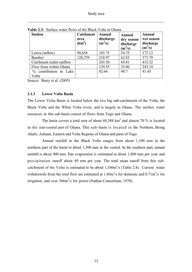
2.1.3 Lower Volta Basin
The Lower Volta Basin is located below the two big sub-catchments of the Volta, the
Black Volta and the White Volta rivers, and is largely in Ghana. The surface water
resources in this sub-basin consist of flows from Togo and Ghana.
The basin covers a total area of about 68,588 km2 and almost 70 % is located
in the east-central part of Ghana. This sub-basin is located in the Northern, Brong
Ahafo, Ashanti, Eastern and Volta Regions of Ghana and parts of Togo.
Annual rainfall in the Black Volta ranges from about 1,100 mm in the
northern part of the basin to about 1,500 mm in the central. In the southern part, annual
rainfall is about 900 mm. Pan evaporation is estimated at about 1,800 mm per year and
precipitation runoff about 89 mm per year. The total mean runoff from this sub-
catchment of the Volta is estimated to be about 1,160m3/s (Table 2.4). Current water
withdrawals from the total flow are estimated at 1.86m3/s for domestic and 0.71m3/s for
irrigation, and over 566m3/s for power (Nathan Consortium, 1970).
Study area
______________________________________________________________________
14
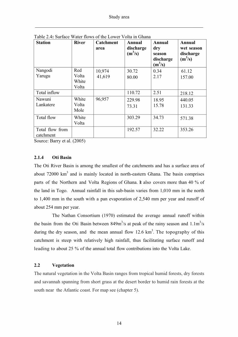
Table 2.4: Surface Water flows of the Lower Volta in Ghana Station River Catchment
area Annual discharge (m3/s)
Annual dry season discharge (m3/s)
Annual wet season discharge (m3/s)
Nangodi Yarugu
Red Volta White Volta
10,974 41,619
30.72 80.00
0.34 2.17
61.12 157.00
Total inflow 110.72 2.51 218.12 Nawuni Lankatere
White Volta Mole
96,957 229.98 73.31
18.95 15.78
440.05 131.33
Total flow White Volta
303.29 34.73 571.38
Total flow from catchment
192.57 32.22 353.26
Source: Barry et al. (2005)
2.1.4 Oti Basin
The Oti River Basin is among the smallest of the catchments and has a surface area of
about 72000 km3 and is mainly located in north-eastern Ghana. The basin comprises
parts of the Northern and Volta Regions of Ghana. It also covers more than 40 % of
the land in Togo. Annual rainfall in this sub-basin varies from 1,010 mm in the north
to 1,400 mm in the south with a pan evaporation of 2,540 mm per year and runoff of
about 254 mm per year.
The Nathan Consortium (1970) estimated the average annual runoff within
the basin from the Oti Basin between 849m3/s at peak of the rainy season and 1.1m3/s
during the dry season, and the mean annual flow 12.6 km3. The topography of this
catchment is steep with relatively high rainfall, thus facilitating surface runoff and
leading to about 25 % of the annual total flow contributions into the Volta Lake.
2.2 Vegetation
The natural vegetation in the Volta Basin ranges from tropical humid forests, dry forests
and savannah spanning from short grass at the desert border to humid rain forests at the
south near the Atlantic coast. For map see (chapter 5).
Study area
______________________________________________________________________
15
____ Volta boundaries
------ iso-zones
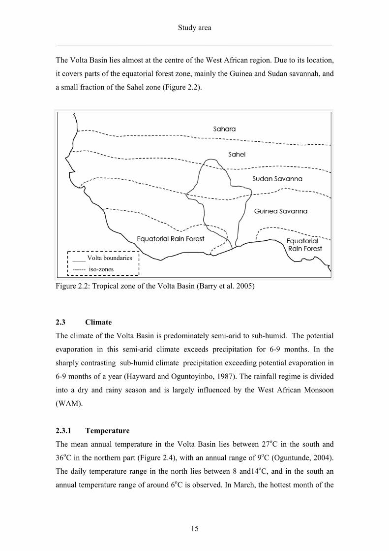
The Volta Basin lies almost at the centre of the West African region. Due to its location,
it covers parts of the equatorial forest zone, mainly the Guinea and Sudan savannah, and
a small fraction of the Sahel zone (Figure 2.2).
Figure 2.2: Tropical zone of the Volta Basin (Barry et al. 2005)
2.3 Climate
The climate of the Volta Basin is predominately semi-arid to sub-humid. The potential
evaporation in this semi-arid climate exceeds precipitation for 6-9 months. In the
sharply contrasting sub-humid climate precipitation exceeding potential evaporation in
6-9 months of a year (Hayward and Oguntoyinbo, 1987). The rainfall regime is divided
into a dry and rainy season and is largely influenced by the West African Monsoon
(WAM).
2.3.1 Temperature
The mean annual temperature in the Volta Basin lies between 27oC in the south and
36oC in the northern part (Figure 2.4), with an annual range of 9oC (Oguntunde, 2004).
The daily temperature range in the north lies between 8 and14oC, and in the south an
annual temperature range of around 6oC is observed. In March, the hottest month of the
Study area
______________________________________________________________________
16
year in the basin, temperatures in the southern parts may rise from a mean of 24oC to
30oC in August (Figure 2.3). The daily temperature range in this area is about 3-5oC
(Hayward and Oguntoyinbo, 1987).
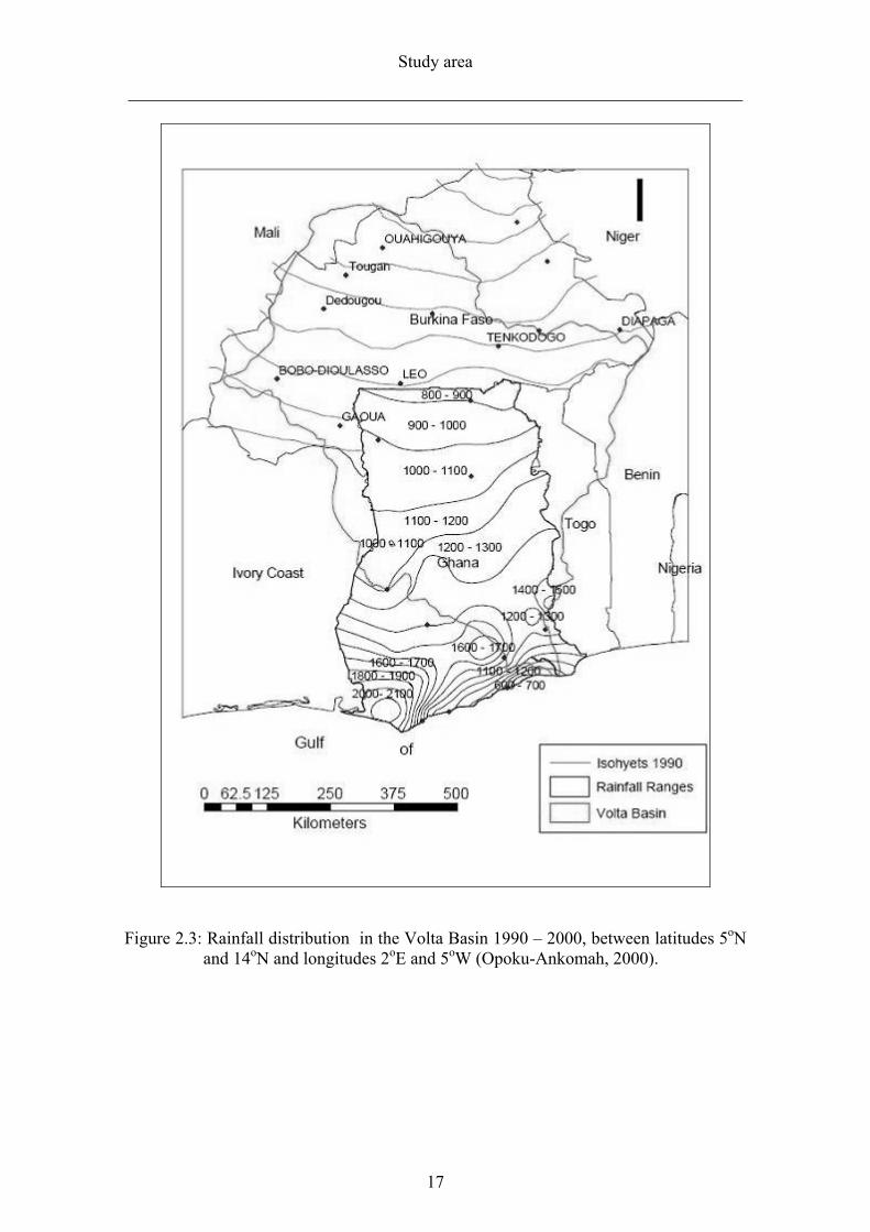
2.3.2 Precipitation
The three climatic zones in the Volta Basin are1) the tropical climate covering over 50
% of the basin (north of latitude 9° N), with one rainfall season peaking in August, 2)
the humid south with two distinct rainy seasons, and3) the tropical transition zone with
two rainfall seasons very close to each other ( south of Latitude 9oN). The high
average annual rainfall variation of 1,600 mm in the south-eastern section of the basin
(Ghana), to about 360 mm in the northern part (Burkina Faso) shows a strong north-
south gradient, with higher rainfall amounts in the tropical South and smaller amounts
in the semi-arid north (Figure 2.3 and 2.4). In the south-western corner of Ghana at the
edge of the Volta Basin annual precipitation exceeding 2,100 mm, whereas in the south-
eastern areas it is less than 800 mm. This is an indication that not only a North-South
gradient is apparent, but also a strong west-east gradient (Figure 2.3). According to
Opoku-Ankomah (2000), since the 1970s there have been a number of changes in the
precipitation patterns in some sub-catchments in the basin, with corresponding rainfall
and run-off reduction. Some areas now have only one rainfall season compared to the
bi-modal system of the past, with the second minor season becoming very weak or non-
existent. Agriculture practiced in the basin, which is rainfed is also shifting from two-
season cropping to single season cropping is evidence of this process.
Around 80 % of annual rainfall occurs from July to September with the
monsoonal rains.
Study area
______________________________________________________________________
17
Figure 2.3: Rainfall distribution in the Volta Basin 1990 – 2000, between latitudes 5oN and 14oN and longitudes 2oE and 5oW (Opoku-Ankomah, 2000).
Study area
______________________________________________________________________
18
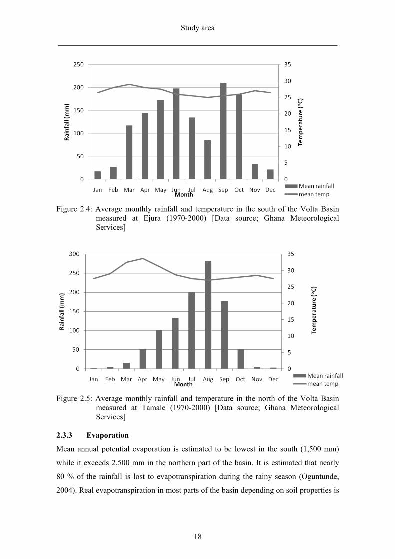
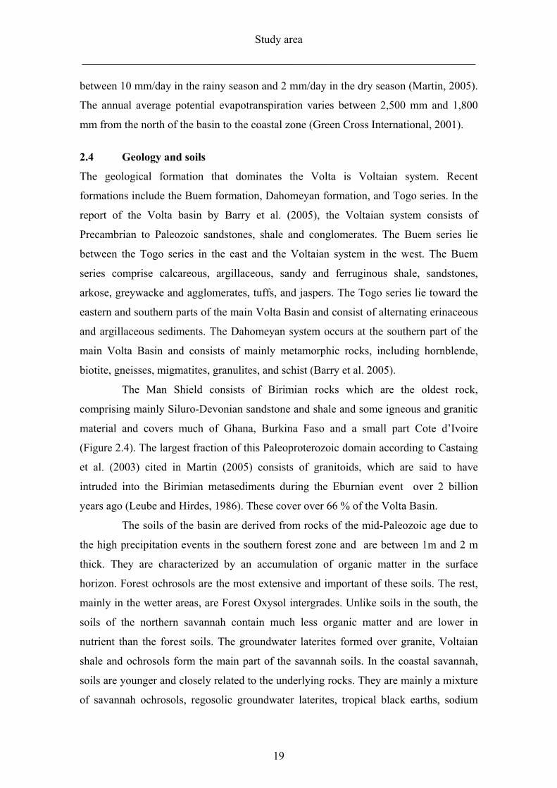
Figure 2.4: Average monthly rainfall and temperature in the south of the Volta Basin measured at Ejura (1970-2000) [Data source; Ghana Meteorological Services]
Figure 2.5: Average monthly rainfall and temperature in the north of the Volta Basin measured at Tamale (1970-2000) [Data source; Ghana Meteorological Services]
2.3.3 Evaporation
Mean annual potential evaporation is estimated to be lowest in the south (1,500 mm)
while it exceeds 2,500 mm in the northern part of the basin. It is estimated that nearly
80 % of the rainfall is lost to evapotranspiration during the rainy season (Oguntunde,
2004). Real evapotranspiration in most parts of the basin depending on soil properties is
Study area
______________________________________________________________________
19
between 10 mm/day in the rainy season and 2 mm/day in the dry season (Martin, 2005).
The annual average potential evapotranspiration varies between 2,500 mm and 1,800
mm from the north of the basin to the coastal zone (Green Cross International, 2001).
2.4 Geology and soils
The geological formation that dominates the Volta is Voltaian system. Recent
formations include the Buem formation, Dahomeyan formation, and Togo series. In the
report of the Volta basin by Barry et al. (2005), the Voltaian system consists of
Precambrian to Paleozoic sandstones, shale and conglomerates. The Buem series lie
between the Togo series in the east and the Voltaian system in the west. The Buem
series comprise calcareous, argillaceous, sandy and ferruginous shale, sandstones,
arkose, greywacke and agglomerates, tuffs, and jaspers. The Togo series lie toward the
eastern and southern parts of the main Volta Basin and consist of alternating erinaceous
and argillaceous sediments. The Dahomeyan system occurs at the southern part of the
main Volta Basin and consists of mainly metamorphic rocks, including hornblende,
biotite, gneisses, migmatites, granulites, and schist (Barry et al. 2005).
The Man Shield consists of Birimian rocks which are the oldest rock,
comprising mainly Siluro-Devonian sandstone and shale and some igneous and granitic
material and covers much of Ghana, Burkina Faso and a small part Cote d’Ivoire
(Figure 2.4). The largest fraction of this Paleoproterozoic domain according to Castaing
et al. (2003) cited in Martin (2005) consists of granitoids, which are said to have
intruded into the Birimian metasediments during the Eburnian event over 2 billion
years ago (Leube and Hirdes, 1986). These cover over 66 % of the Volta Basin.
The soils of the basin are derived from rocks of the mid-Paleozoic age due to
the high precipitation events in the southern forest zone and are between 1m and 2 m
thick. They are characterized by an accumulation of organic matter in the surface
horizon. Forest ochrosols are the most extensive and important of these soils. The rest,
mainly in the wetter areas, are Forest Oxysol intergrades. Unlike soils in the south, the
soils of the northern savannah contain much less organic matter and are lower in
nutrient than the forest soils. The groundwater laterites formed over granite, Voltaian
shale and ochrosols form the main part of the savannah soils. In the coastal savannah,
soils are younger and closely related to the underlying rocks. They are mainly a mixture
of savannah ochrosols, regosolic groundwater laterites, tropical black earths, sodium
Study area
______________________________________________________________________
20
vleisols, tropical grey earths and acid gleisols and are generally poor largely because of
inadequate moisture.
The soils of the northern part (Burkina Faso) are largely lateritic compared to
the southern part of the Basin (Ghana), where they are of the lixisol type. According to
Adams et al. (1996), the weathered soils are usually a composition of kaolinite clays
and have high contents of iron, aluminium and titanium oxide. The aggregate stability at
the surfaces is usually low, and soils with low vegetation cover are prone to erosion.
The other main group of soils in the Volta Basin consists of arenosols, mainly
found in the arid north of the basin. They are basically sandy and coated with iron
oxides, which gives the soil its specific reddish color. These soils are characterized by
high infiltration rates. A study on soil properties conducted by Agyare (2004) revealed
high discrepancies between subsoil and topsoil due to less soil disturbance in the
subsoils. The computed saturated hydraulic conductivity (Ksat) is a high variability in
space for the soil layers considered. Another study by Giertz (2004) cited in Jung (2006)
supports these findings.
Study area
______________________________________________________________________
21
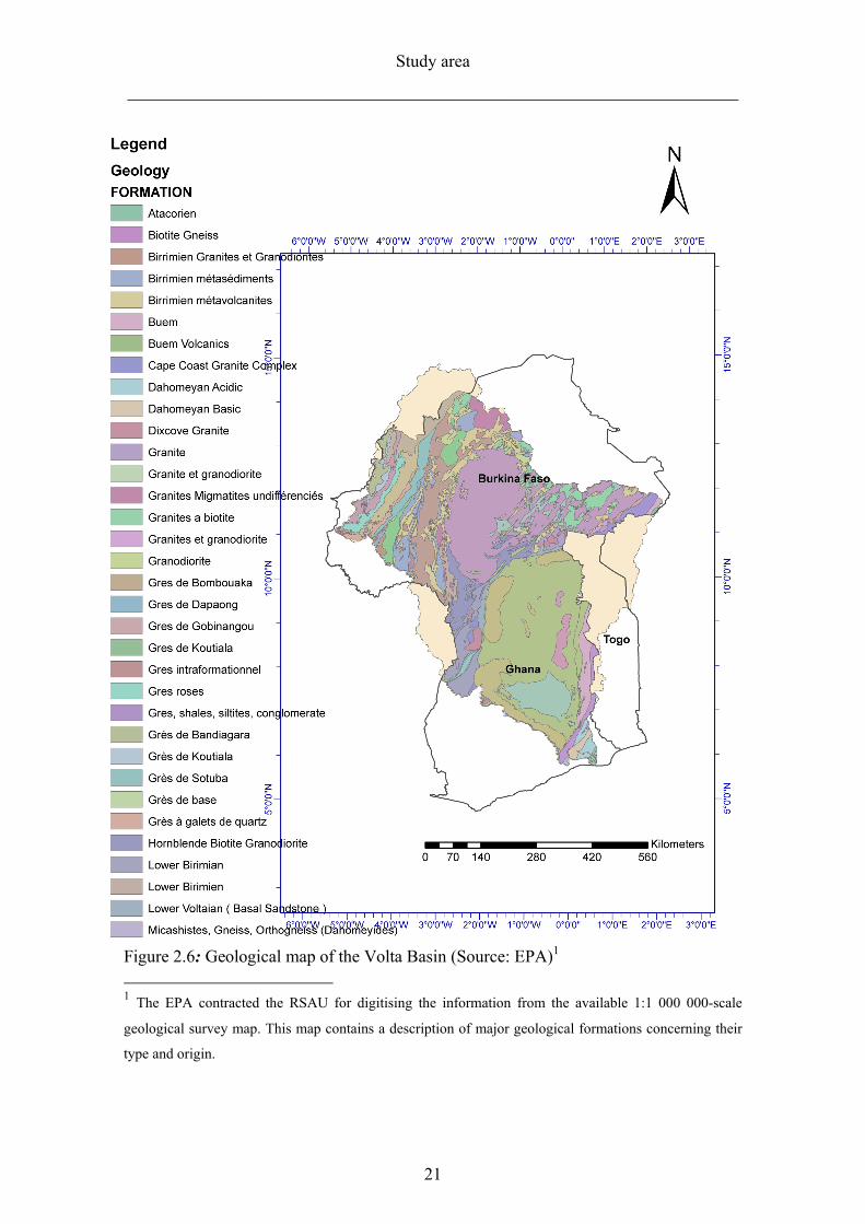
Figure 2.6: Geological map of the Volta Basin (Source: EPA)1
1 The EPA contracted the RSAU for digitising the information from the available 1:1 000 000-scale
geological survey map. This map contains a description of major geological formations concerning their
type and origin.
Study area
______________________________________________________________________
22
2.5 Land use and agriculture
Increasing population growth all over the Volta Basin is leading to an increasing
pressure on agricultural land for food production. Most Farmers have therefore
abandoned the original farming practice of shifting cultivation with long fallow periods
because it is viewed to be less viable and unpractical. Some of the crops cultivated on
uplands are maize (Zea mays), sorghum (Sorghum bicolor), groundnut (Arachis
hypogaea), cowpea (Vigna unguiculata), with rice (Oryza spp.) grown in valley
bottoms. The majority of the farms are small-scale subsistence farms and these are only
a few commercial farms. Traditional shifting cultivation with land rotation is practiced
to some extent across the basin.
Livestock production on a small and large scale is important for the livelihood
of the people in the basin. Mostly, the family owns cattle with the family head having
the direct responsibility for the animals in the north, while poultry and farming on pig
on a commercial scale are practiced in the south. The livestock mostly owned by
household are sheep, goat, and birds.
2.6 Hydrology and water resources
Apart from the huge network of rivers, the basin is dotted with a number reservoirs,
ponds and dugouts. In areas where surface water is inadequate, groundwater resources
are used by the small communities for domestic and irrigation purposes. According to
the World Bank report (1992), groundwater resources are of relatively good quality and
usually only need minimum treatment. Many communities within the basin depend
largely on groundwater for their water needs. Data is scanty on groundwater level
fluctuation and recharge, but in some areas a high recharge is observed.
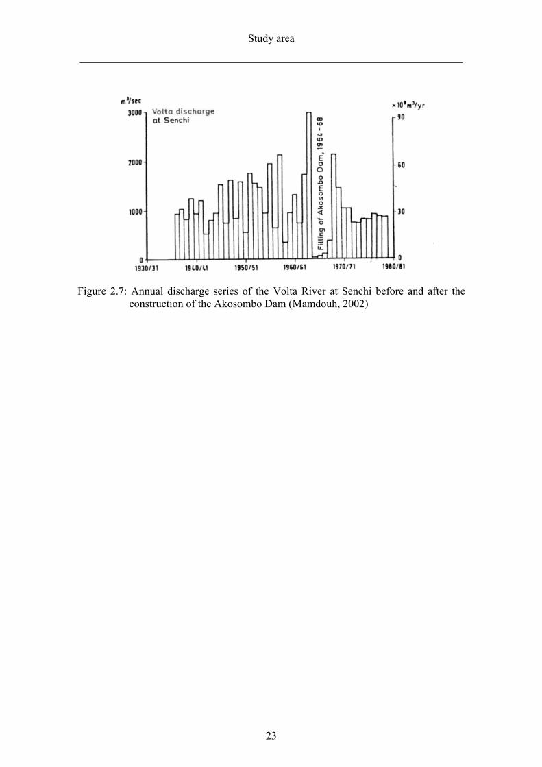
Runoff is essential for hydropower generation, which is a major source of
energy for the countries within the basin. Reduction in flows has rendered the
hydropower systems vulnerable, and this shows no sign of ending soon. Since the
Akosombo hydro-electric dam was constructed, discharge has barely reached 1000 m3/s,
and recent records show a further decline (Figure 2.5).
Study area
______________________________________________________________________
23
Figure 2.7: Annual discharge series of the Volta River at Senchi before and after the construction of the Akosombo Dam (Mamdouh, 2002)
Climatological and hydrological data
______________________________________________________________________
24
3 CLIMATOLOGICAL AND HYDROLOGICAL DATA
3.1 Data availability
Until the beginning of the last decade, little was known about what data exist for the
Volta Basin with regards to Meteorological and hydrological, and what time periods
they represent. In the GLOWA-Volta project; the analysis of the physical and socio-
economic determinants of the hydrological cycle of the Volta Basin created the
umbrella under which a number of PhD scientific researchers were conducted. For
example, within the framework of the Volta Project, Martin (2005) studied on a
watershed within the White Volta, Jung (2006) in the “Regional Climate Change and
the Impact on Hydrology in the Volta Basin of West Africa” considered the entire basin
and focused more on the Burkina Faso and the northern parts of the Volta Basin while
Wagner (2008) used data from the Ghana part of White Volta. Recent reports and
publications based on archived data highlight the availability of some collected and
archived data in the countries within the basin. At the beginning of this research, the
data base of GLOWA Volta had scant information for areas outside previous research
sites. Little was known about what may have been achieved in these areas for the
desired periods of 1961-2007 to synchronize with the already cleaned data of pervious
work. This time series is essential for this research because for any useful comparison of
conditions of the past and the future, a good presentation of the meteorological and
hydrological data is needed. Although some models are sometimes able to generate
data, they have often failed to simulate most extremes (e.g. temperature, rainfall etc)
correctly, hence archived gauged data is preferred for this study. Initial assessment of
the data archived by national agencies showed that continuous meteorological data for
the basin for long periods was lacking, and where data existed, the quality was
questionable with large gaps of missing data. After the initial sorting of the available
data for the basin, data from gauges that could be used were widely spaced. Available
monthly and daily data from meteorological stations monitored solely by the
metrological services of both Ghana and Burkina Faso needed some verification and
quality checks. Information from the hydrological services also revealed that most of
the rivers were previously ungauged; hence no run-off data exist for such rivers. On the
whole, continuous stream discharge measurements data at daily intervals were available
Climatological and hydrological data
______________________________________________________________________
25
for some stations in Ghana and Burkina Faso, also with some gaps and questionable
values that needed attention.
3.1.1 Data quality assessment
The quality of the data determines to a great extent the hydrological model efficiency
and hence the conclusions that can be drawn from the modeling results.
Data which many human hands have handled in different locations and spanning many
years are bound to have some problems with quality. This is more so the case when the
data are influenced by human activities in almost all the stages of production. In
situations like these, Beven (2002) cautioned that models will not be able to simulate
accurate predictions if the areal precipitation is not adequately represented. In
developing countries such as those in West Africa, hydro- meteorology data are
collected and recorded manually. Digitizing these large amounts of data by poorly
trained people also leads to quality problems.
The quality of any measured parameter depends on precision and accuracy,
where the former is associated with how close and reproducible the measured value is
from a repeated measurement if there were to be one, whereas the latter is focused on
how good the measured value agrees with the true value. However, natural irregularities
or differences in what is being measured must not be considered as errors. This thus
demands a careful approach in error analysis of large amounts of data of a cast area that
has high variation in hydrology and climate (Bevington, 1992). This renders most
statistical methods that are based on normal distributions useless in this analysis.
Errors may occur because of gauge management, human errors in reading
and/or recording or typing errors in digitizing data from data sheets. The latter causes by
far the greatest error and is usually the case. Underestimation of the gauge catch
compared to the ground catch may be as high as 100 % and more (UNESCO, 1978
referred to in Herschy, 1999).
Errors limited to gauges management are those where gauges malfunction due
to poor maintenance such as cleaning, and recalibration among others. Other
uncertainties may be due to poor reading of the equipment. Since data were collected
manually, an error in reading measurement automatically introduced an error. In
situations where data was correctly read, a different value could be recorded, such as
Climatological and hydrological data
______________________________________________________________________
26
placing a decimal point in the wrong place. Human error in entering the data into a
spreadsheet brought along some errors as typing errors. As these uncertainties usually
do not show regular patterns, correcting such errors becomes more difficult when
comparing data with other neighboring station data, where different conditions apply,
data values might differ immensely.
Three steps were taken for verifying the data used in this research:
visualization, comparison to nearby stations within the same zone, and regression. Base
knowledge of the area was essential for visually picking out doubtful data. Personnel
from the respective organization of the countries were contacted on data that were
abnormal with respect to the long term data set of the stations. The data was accepted
when adequate reasons were given for such data sets to differ that much from the
normal values.
Comparing neighboring stations for data verification required that squall lines
of rainfall were considered to enable the assessment of these data to be related and
compared. Rainfall amounts from neighboring stations during a rainy event from the
same squall line would not necessarily be equal but would show some relative
magnitudes.
Station data was always regressed with the long-term data of the same station,
and though season change and seasonal averages change, outliers offer some ideas
regarding unusual occurrences to stations.
3.2 Climate data
This research demanded a variety of input data most especially climate information.
Data used heavily relied on collected historical data that were available and accessible
to the GLOWA Volta project (GVP). A memorandum of agreement signed between
GLOWA Volta project and the national agencies allowed access and use of the data for
this research. Priority was put on stations across the regions where data was lacking in
the data base of GLOWA Volta project but required for this research. Some of the
historical data from some stations existed in handwritten papers and had to be entered
into a spreadsheet to facilitate processing. From the large pool of stations with data,
stations were selected according to the criteria that the location of the station was not in
the catalogue of station of GVP and in a region that did not have a good concentration
Climatological and hydrological data
______________________________________________________________________
27
or distribution of gauged stations within the catchment in the catalogue. A considerable
part of the research area is covered by protected national parks in Ghana (Mole) and
Burkina Faso; hence data does not come from these parts of the research area. The
nearest stations to these parks were used for interpolation.
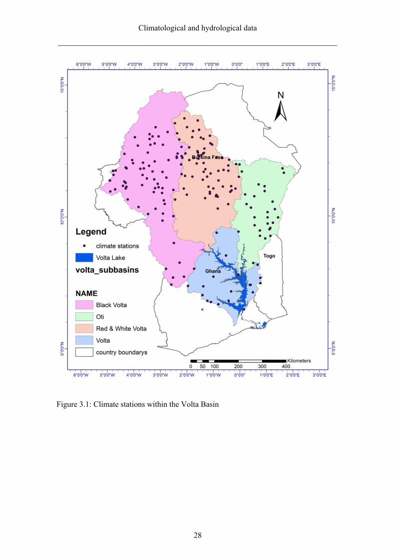
3.2.1 Meteorological agencies
The Ghana Meteorological Department; now called Ghana Meteorological Agency
(GMA) is the major source of the meteorological data used in this research. Most of the
historical daily data covered from 1961 to 2004. The GMA operated two types of
stations: 1) the synoptic stations; record data for temperature, relative humidity,
sunshine duration, pan evaporation and wind speed (Figure 3.1) and 2) rain gauge
stations that were dotted around synoptic stations mainly to monitor rainfall amount
over an area. Additional meteorological data was obtained from the meteorological
agency in Burkina Faso for stations that were needed from the Burkina Faso part of the
basin. The list of stations selected for this research (table 3.1) shows locations at a range
of different distances and elevations.
Climatological and hydrological data
______________________________________________________________________
28
Figure 3.1: Climate stations within the Volta Basin
Climatological and hydrological data
______________________________________________________________________
29
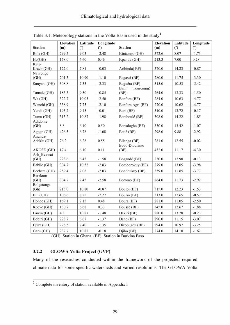
Table 3.1: Meteorology stations in the Volta Basin used in the study2
Station Elevation (m)
Latitude (o)
Longitude (o) Station
Elevation (m)
Latitude (o)
Longitude (o)
Bole (GH) 299.5 9.03 -2.48 Kintampo (GH) 372.6 8.07 -1.73
Ho(GH) 158.0 6.60 0.46 Kpandu (GH) 213.3 7.00 0.28 Kete-Krachi(GH) 122.0 7.81 -0.03 Aribinda( BF) 370.0 14.23 -0.87 Navrongo (GH) 201.3 10.90 -1.10 Bagassi (BF) 280.0 11.75 -3.30
Sunyani (GH) 308.8 7.33 -2.33 Baguéra (BF) 315.0 10.53 -5.42
Tamale (GH) 183.3 9.50 -0.85 Bam (Tourcoing) (BF) 264.0 13.33 -1.50
Wa (GH) 322.7 10.05 -2.50 Banfora (BF) 284.0 10.63 -4.77
Wenchi (GH) 338.9 7.75 -2.10 Banfora Agri (BF) 270.0 10.62 -4.77
Yendi (GH) 195.2 9.45 -0.01 Bani (BF) 310.0 13.72 -0.17
Tumu (GH) 313.2 10.87 -1.98 Baraboulé (BF) 308.0 14.22 -1.85 Adidome (GH) 8.8 6.10 0.50 Barsalogho (BF) 330.0 13.42 -1.07
Agogo (GH) 426.5 6.78 -1.08 Batié (BF) 298.0 9.88 -2.92 Ahunda-Adaklu (GH) 76.2 6.28 0.55 Bilanga (BF) 281.0 12.55 -0.02
AKUSE (GH) 17.4 6.10 0.11 Bobo-Dioulasso (BF) 432.0 11.17 -4.30
Ash_Bekwai (GH) 228.6 6.45 -1.58 Bogandé (BF) 250.0 12.98 -0.13
Babile (GH) 304.7 10.52 -2.83 Bomborokuy (BF) 279.0 13.05 -3.98
Bechem (GH) 289.4 7.08 -2.03 Bondoukuy (BF) 359.0 11.85 -3.77 Berekum (GH) 304.7 7.45 -2.58 Boromo (BF) 264.0 11.73 -2.92 Bolgatanga (Gh) 213.0 10.80 -0.87 Boulbi (BF) 315.0 12.23 -1.53
Bui (GH) 106.6 8.25 -2.27 Boulsa (BF) 313.0 12.65 -0.57
Hohoe (GH) 169.1 7.15 0.48 Boura (BF) 281.0 11.05 -2.50
Kpeve (GH) 130.7 6.68 0.33 Boussé (BF) 345.0 12.67 -1.88
Lawra (GH) 4.8 10.87 -1.48 Dakiri (BF) 280.0 13.28 -0.23
Bobiri (GH) 228.7 6.67 -1.37 Dano (BF) 290.0 11.15 -3.07
Ejura (GH) 228.5 7.40 -1.35 Diébougou (BF) 294.0 10.97 -3.25
Garu (GH) 237.7 10.85 -0.18 Djibo (BF) 274.0 14.10 -1.62 (GH): Station in Ghana, (BF): Station in Burkina Faso
3.2.2 GLOWA Volta Project (GVP)
Many of the researches conducted within the framework of the projected required
climate data for some specific watersheds and varied resolutions. The GLOWA Volta
2 Complete inventory of station available in Appendix I
Climatological and hydrological data
______________________________________________________________________
30
project setup automated observation stations in three locations in the Ghana part of the
basin: Ejura in the transition zone, Tamale in the guinea savannah zone and Navrongo
in the Sudan savannah zone. In a 10mim interval, a Campbell automated data loggers
monitored and recorded temperature, relative humidity, net and global radiation, wind
speed and direction, soil heat at 5cm and 10cm, atmospheric pressure and precipitation.
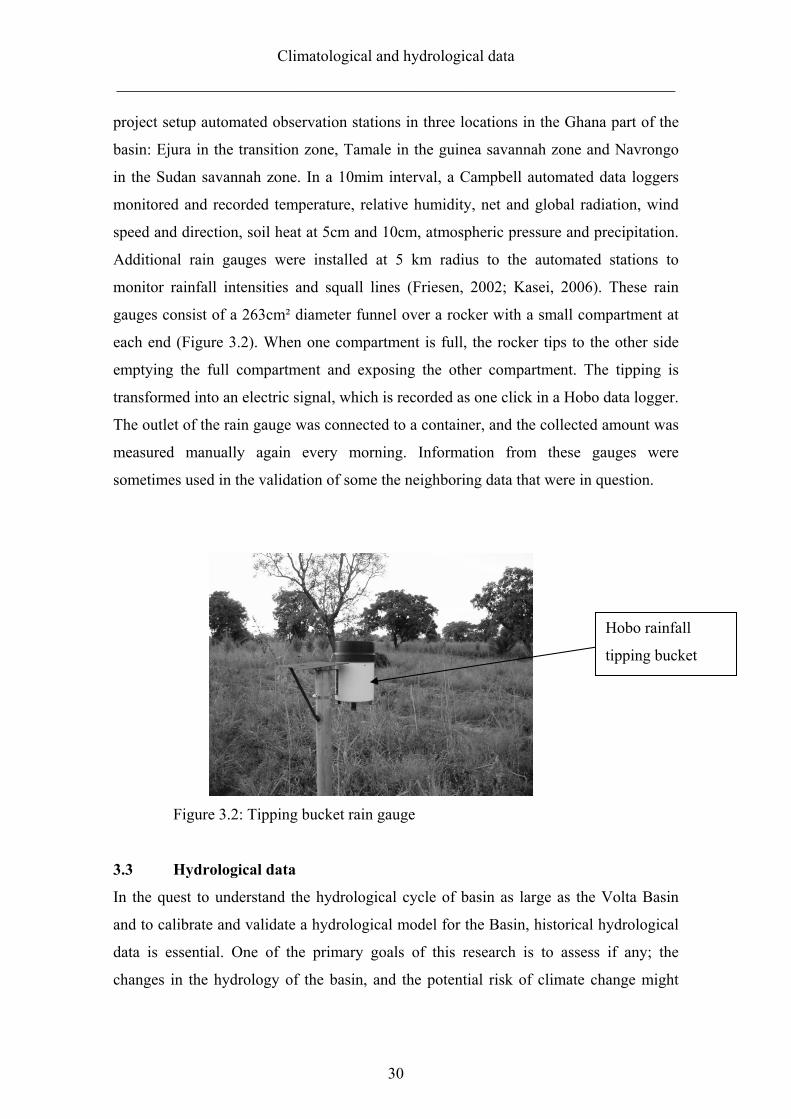
Additional rain gauges were installed at 5 km radius to the automated stations to
monitor rainfall intensities and squall lines (Friesen, 2002; Kasei, 2006). These rain
gauges consist of a 263cm² diameter funnel over a rocker with a small compartment at
each end (Figure 3.2). When one compartment is full, the rocker tips to the other side
emptying the full compartment and exposing the other compartment. The tipping is
transformed into an electric signal, which is recorded as one click in a Hobo data logger.
The outlet of the rain gauge was connected to a container, and the collected amount was
measured manually again every morning. Information from these gauges were
sometimes used in the validation of some the neighboring data that were in question.
Figure 3.2: Tipping bucket rain gauge
3.3 Hydrological data
In the quest to understand the hydrological cycle of basin as large as the Volta Basin
and to calibrate and validate a hydrological model for the Basin, historical hydrological
data is essential. One of the primary goals of this research is to assess if any; the
changes in the hydrology of the basin, and the potential risk of climate change might
Hobo rainfall
tipping bucket
Climatological and hydrological data
______________________________________________________________________
31
have impact on the water resources of the Volta Basin. Flow data is required to calibrate
and validate models that are expected to mimic the water balance of the basin.
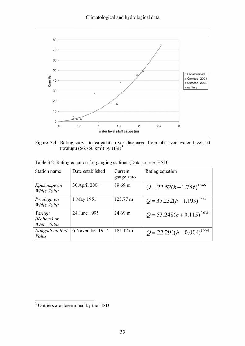
3.3.1 Hydrological Service Department
The Hydrological Services Department (HSD) of Ghana is the only source of the
hydrological data used in this research since data required to compare with model
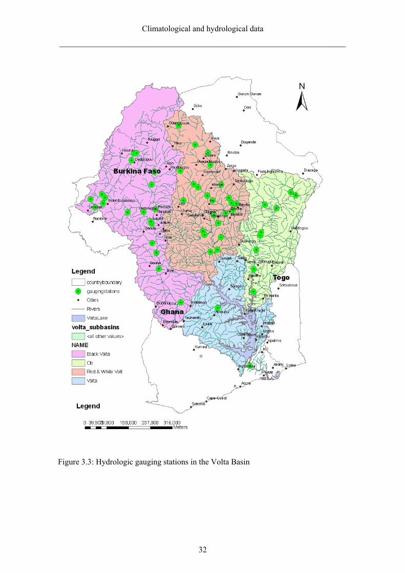
outputs were mainly within Ghana. GVP catalogued all hydrological stations within the
basin (Figure 3.3) and sorted historical data with most spanning from 1961 till 2006; a
few dating far back as 1951. The HSD installed staff gauges in streams and manually
measured the water level daily. Calculating discharge for any water level; the HSD
developed a stage discharge relationship which is expressed in an exponential rating
curve. (The rating equations vary slightly from one station to another (Table 3.2).
Data used in this research had gaps for most of the stations that had been
retrieved. Attempts to fill some of the gaps with mathematical algorithms developed by
Amisigo (2005) was successful for some catchments but were not used in this research.
Climatological and hydrological data
______________________________________________________________________
32
Figure 3.3: Hydrologic gauging stations in the Volta Basin
Climatological and hydrological data
______________________________________________________________________
33
Figure 3.4: Rating curve to calculate river discharge from observed water levels at Pwalugu (56,760 km2) by HSD3
Table 3.2: Rating equation for gauging stations (Data source: HSD)
Station name Date established Current gauge zero
Rating equation
Kpasinkpe on White Volta
30 April 2004 89.69 m 566.1)786.1(52.22 hQ
Pwalugu on White Volta
1 May 1951 123.77 m 593.1)193.1(252.35 hQ
Yarugu (Kobore) on White Volta
24 June 1995
24.69 m 030.2)115.0(248.53 hQ
Nangodi on Red Volta
6 November 1957 184.12 m 774.1)004.0(291.22 hQ
3 Outliers are determined by the HSD

Climatological and hydrological data
______________________________________________________________________
34
3.3.2 GLOWA Volta Project
Wagner (2008) installed two gauges in Pwalugu and Yarugu both in the White Volta to
obtain additional discharge data for hydrological modeling of the White Volta. Hydro
Argos systems were also installed in cooperation with the HSD in Ghana in order to
contribute to the Volta Hycos System. Additionally Martin (2005) instrumented the
Atankwidi (White Volta) catchment with water level recording. This data is available in
the data base of the GVP but were not used in this research.
Methodology
______________________________________________________________________
35
4 METHODOLOGY
Hydrological modeling usually is a physically-based distributed-parameter system,
developed in an attempt to simulate the hydrologic processes such as the transformation
of precipitation to runoff, and response of watershed and river basins to those processes.
Flow simulations over the years have ranged from very simple antecedent precipitation
and tank models to very complex nested and distributed parameter models such as the
European Hydrological system model (SHE) and the Hydrologic Simulation Program
Fortran (HSPF) (Maidment, 1992). Hydrological simulation models are often used to
provide information on the interaction between water and land resources to aid in
decision making, usually regarding the development and management of the scarce
resources. Traditionally, hydrologic models have considered the watersheds as
homogeneous against the complex terrain in which they are applied (Kilgore, 1997).
These processes are sometimes described by differential equations based on simplified
hydraulic laws with other processes, which may be expressed by empirical algebraic
equations (Arnold et al. 1998). Hydrological simulation modeling systems are usually
classified in three main groups namely: empirical black box, lumped conceptual, and the
distributed physically-based systems. The great majority of the modeling systems used
in practice today belongs to the empirical black box and lumped conceptual systems,
which are known to be relatively simple and require a small number of parameters
(approximately 5-10) to calibrate. Despite their simplicity, many models have proven to
be quite successful in representing the hydraulics of watersheds (Refsgaard et al. 1996).
Hydrological models have been developed in recent times to incorporate the
heterogeneity of the watershed such as the spatial distribution of various boundary
conditions of topography, vegetation, land use, soil characteristics, rainfall, and
temperature among others. The results have been detailed spatial outputs such as soil
moisture grids, groundwater fluxes and many more (Troch et al. 2003). According to
Schulla (1999), the WaSiM used in this study is capable of incorporating spatial
heterogeneity in its analyses and is also built to be sensitive to the grid size of large
watersheds of varied topography and with used success in the investigation of
mountainous basins such as the Thur Basin with an area of 1700 km². The Water
balance- Simulation-Model WaSiM-ETH is regarded as one of the models that
Methodology
______________________________________________________________________
36
adequately describe the major processes of evaporation, canopy interception,
transpiration, snowmelts, saturated and unsaturated sub flows, and channel/routed flow.
One major bottleneck for many hydrological models according to Jain et al. (1992) and
Troch et al. (2003) is the substantial data requirement for the various processes by these
models.
For an effective modeling for management of the ecology of a watershed such
as one of the goals of this research, thorough understanding of the hydrologic processes
is essential. The complexity of the spatial and temporal variations in soils, vegetation
and land-use practices of the large Volta Basin make it even more difficult. As
suggested by Singh and Woolhiser (2002), mathematical models such as WaSiM and
geospatial analysis tools are needed to comprehensively study the various processes.
4.1 Model selection
A thorough literature review on models used on large watersheds that incorporated land-
use changes, runoff and soil characteristics of watersheds and basins was carried out.
According to Brown and Heuvelink (2005), hydrological models are inherently
imperfect in many ways because they abstract and simplify “real” hydrological patterns
and processes. This imperfection is partly due to the scale of the catchment against the
backdrop that most hydrological modeling is based on regionalization of hydrologic
variables, with constituent process and theories essentially derived at the laboratory or
other small scales (Blöschel, 1996). The underpinned assumption of catchment
homogeneity and uniformity and time invariance of various flow paths over watersheds
and through soils and vegetation underscores the embedded processes such as channel
hydraulics, soil physics and chemistry, groundwater flow, crop micrometeorology, plant
physiology, boundary layer meteorology, etc.(Brown and Heuvelink, 2005). All the
flaws of hydrological modeling notwithstanding, process-based distributed models have
proven to simulate fairly well the spatial variability of the water balance among other
processes when the main hydrological parameters and processes are known
(Schellekens, 2000). Until now, there has not been an alternative to hydrological
simulation of watersheds that incorporate spatial scenarios such as land use changes.
Previous application of the process-based distributed model WaSiM-ETH for
various environments and the proven capabilities were essential for the selection of this
Methodology
______________________________________________________________________
37
model for this study. One major successful use of the model in a challenging
topographic terrain was by Schulla (1997) in the assessment of the impact of climate
change on the hydrological regimes and water of the Thur Basin located in north-east
part of Switzerland. Furthermore, Niehoff (2001) cited in Leemhuis (2005), Jasper et al.
(2002), Gurtz et al. (2003), Verbunt et al. (2003), and Leemhuis (2005) among others
have successfully applied WaSiM-ETH to watersheds of different sizes and structures.
For the arid region of the Volta, WaSiM-ETH was successfully applied by Martin
(2005), Jung (2006) and Wagner (2008).
For this study, the Model WaSiM-ETH after Schulla and Jasper (1999) was
selected, because it has the ability to characterize complex watershed representations to
explicitly account for spatial variability of the soil profiles at the desired resolution
amidst water balance and rainfall distribution in the assessment of changes in
precipitation and runoff over the recent past using historical data.
4.2 Basic concept
The basic concept for the modeling in this study is to provide the spatial and temporal
data over time that reflect and adequately represent the specific physio-geographical
variability and heterogeneity of the Volta River system.
The use of the model WaSiM-ETH focuses on mimicking the hydrology of the
Volta Basin through the reproduction of gauged station hydrographs and subsequently
investigates the impact of changes in climate and/or rainfall anomalies on water
resources over time (Figure 4.1) for the large watershed of the Volta Basin. For a
detailed description of WaSiM-ETH see Chapter 5.
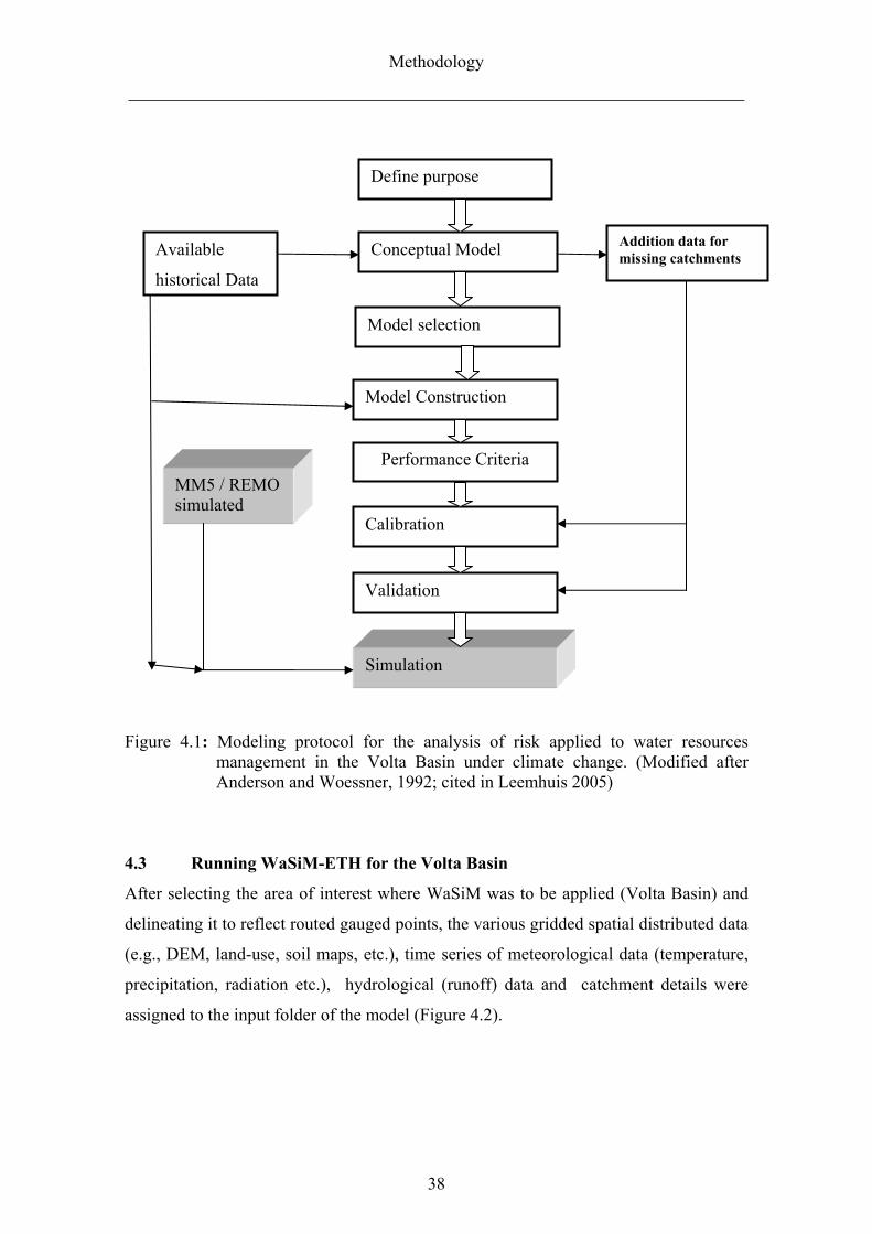
Methodology
______________________________________________________________________
38
Figure 4.1: Modeling protocol for the analysis of risk applied to water resources management in the Volta Basin under climate change. (Modified after Anderson and Woessner, 1992; cited in Leemhuis 2005)
4.3 Running WaSiM-ETH for the Volta Basin
After selecting the area of interest where WaSiM was to be applied (Volta Basin) and
delineating it to reflect routed gauged points, the various gridded spatial distributed data
(e.g., DEM, land-use, soil maps, etc.), time series of meteorological data (temperature,
precipitation, radiation etc.), hydrological (runoff) data and catchment details were
assigned to the input folder of the model (Figure 4.2).
Define purpose
Conceptual Model Addition data for missing catchments
Calibration
Performance Criteria
Model Construction
Model selection
Available
historical Data
Validation
Simulation
MM5 / REMO simulated
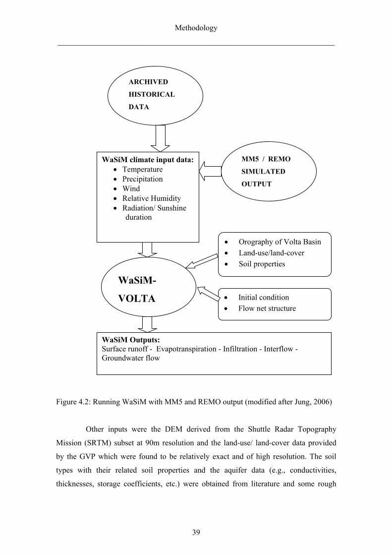
Methodology
______________________________________________________________________
39
Figure 4.2: Running WaSiM with MM5 and REMO output (modified after Jung, 2006)
Other inputs were the DEM derived from the Shuttle Radar Topography
Mission (SRTM) subset at 90m resolution and the land-use/ land-cover data provided
by the GVP which were found to be relatively exact and of high resolution. The soil
types with their related soil properties and the aquifer data (e.g., conductivities,
thicknesses, storage coefficients, etc.) were obtained from literature and some rough
WaSiM climate input data: Temperature Precipitation Wind Relative Humidity Radiation/ Sunshine
duration
WaSiM Outputs: Surface runoff - Evapotranspiration - Infiltration - Interflow - Groundwater flow
Orography of Volta Basin
Land-use/land-cover
Soil properties
ARCHIVED
HISTORICAL
DATA
MM5 / REMO
SIMULATED
OUTPUT
Initial condition
Flow net structure
WaSiM-
VOLTA
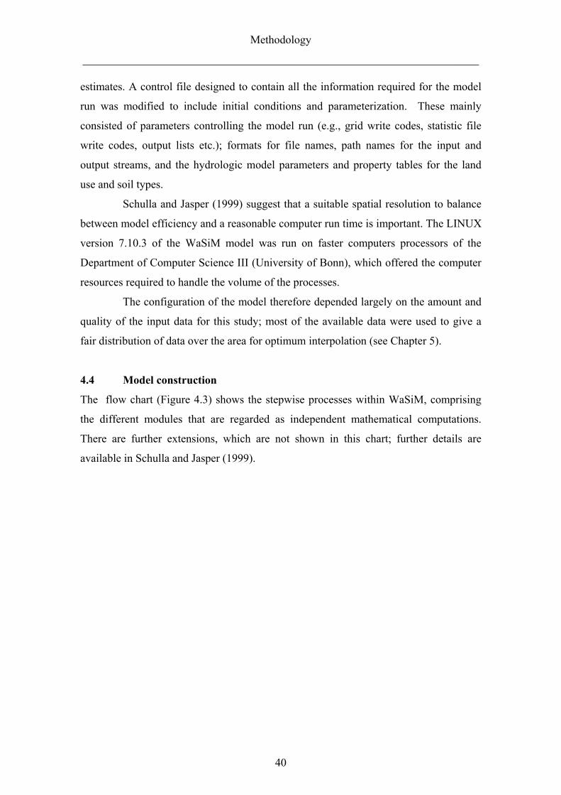
Methodology
______________________________________________________________________
40
estimates. A control file designed to contain all the information required for the model
run was modified to include initial conditions and parameterization. These mainly
consisted of parameters controlling the model run (e.g., grid write codes, statistic file
write codes, output lists etc.); formats for file names, path names for the input and
output streams, and the hydrologic model parameters and property tables for the land
use and soil types.
Schulla and Jasper (1999) suggest that a suitable spatial resolution to balance
between model efficiency and a reasonable computer run time is important. The LINUX
version 7.10.3 of the WaSiM model was run on faster computers processors of the
Department of Computer Science III (University of Bonn), which offered the computer
resources required to handle the volume of the processes.
The configuration of the model therefore depended largely on the amount and
quality of the input data for this study; most of the available data were used to give a
fair distribution of data over the area for optimum interpolation (see Chapter 5).
4.4 Model construction
The flow chart (Figure 4.3) shows the stepwise processes within WaSiM, comprising
the different modules that are regarded as independent mathematical computations.
There are further extensions, which are not shown in this chart; further details are
available in Schulla and Jasper (1999).
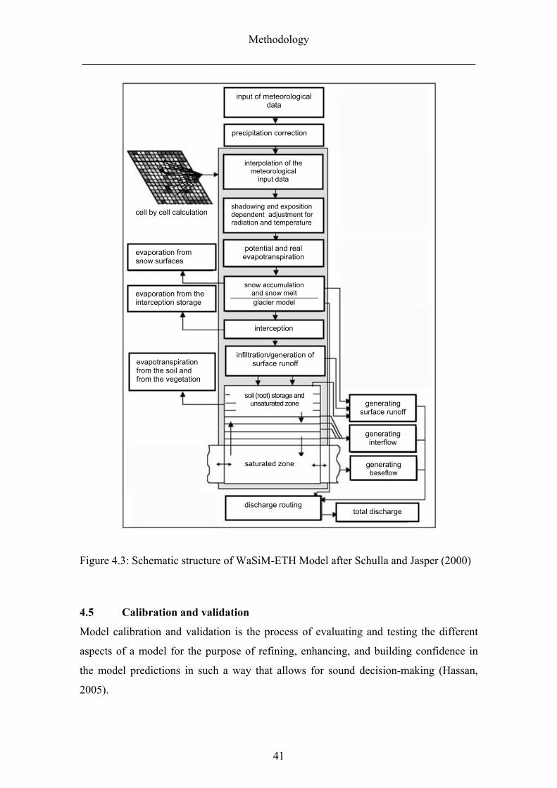
Methodology
______________________________________________________________________
41
Figure 4.3: Schematic structure of WaSiM-ETH Model after Schulla and Jasper (2000)
4.5 Calibration and validation
Model calibration and validation is the process of evaluating and testing the different
aspects of a model for the purpose of refining, enhancing, and building confidence in
the model predictions in such a way that allows for sound decision-making (Hassan,
2005).
evaporation from the interception storage
evaporation from snow surfaces
evapotranspiration from the soil and from the vegetation
cell by cell calculation
soil (root) storage and unsaturated zone
saturated zone
discharge routing
infiltration/generation of surface runoff
interception
snow accumulation and snow melt glacier model
potential and real evapotranspiration
shadowing and exposition dependent adjustment for radiation and temperature
interpolation of the meteorological
input data
precipitation correction
input of meteorological data
generating surface runoff
generating interflow
generating baseflow
total discharge
Methodology
______________________________________________________________________
42
The validation process adopted to sufficiently predict with a satisfactory accuracy was
the split sample test method (see also Xu, 1999). The time series of the period under
investigation is split into a period of model warming, calibration and validation. The
warm-up period is usually at the beginning of the time series and is used by the model
to set up initial conditions for subsequent runs. The calibration procedure is applying
optimum values to the sensitive parameters in order to optimize the predictive ability of
the model. The validation procedure involves applying the calibrated model without
changing any parameter value for another period. Again the model’s performance is
evaluated and is expected to correspond with the accuracy achieved during the
calibration period (Figure 4.4). The model is then regarded as validated and can be used
for predictive analysis thereafter.
The accuracy of the model is mainly assessed by comparing observed
hydrograph versus simulated ones. This comparison is possible either with objective
functions (e.g. Willmott (1981), Nash and Sutcliffe (1970)) or graphically. In general,
the two most common methods of calibration are: the trial-and-error adjustment and
automatic parameter estimation method or a combination of the two methods.
The iteration calibration process (Figure 4.2) followed to successfully reach
the attained values of the calibrated parameter for this study under the set acceptable
statistics.
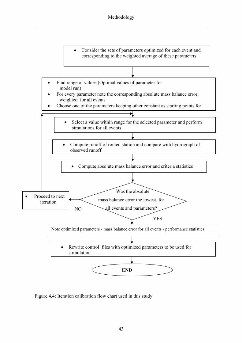
Methodology
______________________________________________________________________
43
NO
YES
Note optimized parameters - mass balance error for all events - performance statistics
Rewrite control files with optimized parameters to be used for stimulation
END
Consider the sets of parameters optimized for each event and corresponding to the weighted average of these parameters
Find range of values (Optimal values of parameter for model run)
For every parameter note the corresponding absolute mass balance error, weighted for all events
Choose one of the parameters keeping other constant as starting points for
Select a value within range for the selected parameter and perform simulations for all events
Compute runoff of routed station and compare with hydrograph of observed runoff
Compute absolute mass balance error and criteria statistics
Proceed to next iteration
Was the absolute
mass balance error the lowest, for
all events and parameters?
Figure 4.4: Iteration calibration flow chart used in this study
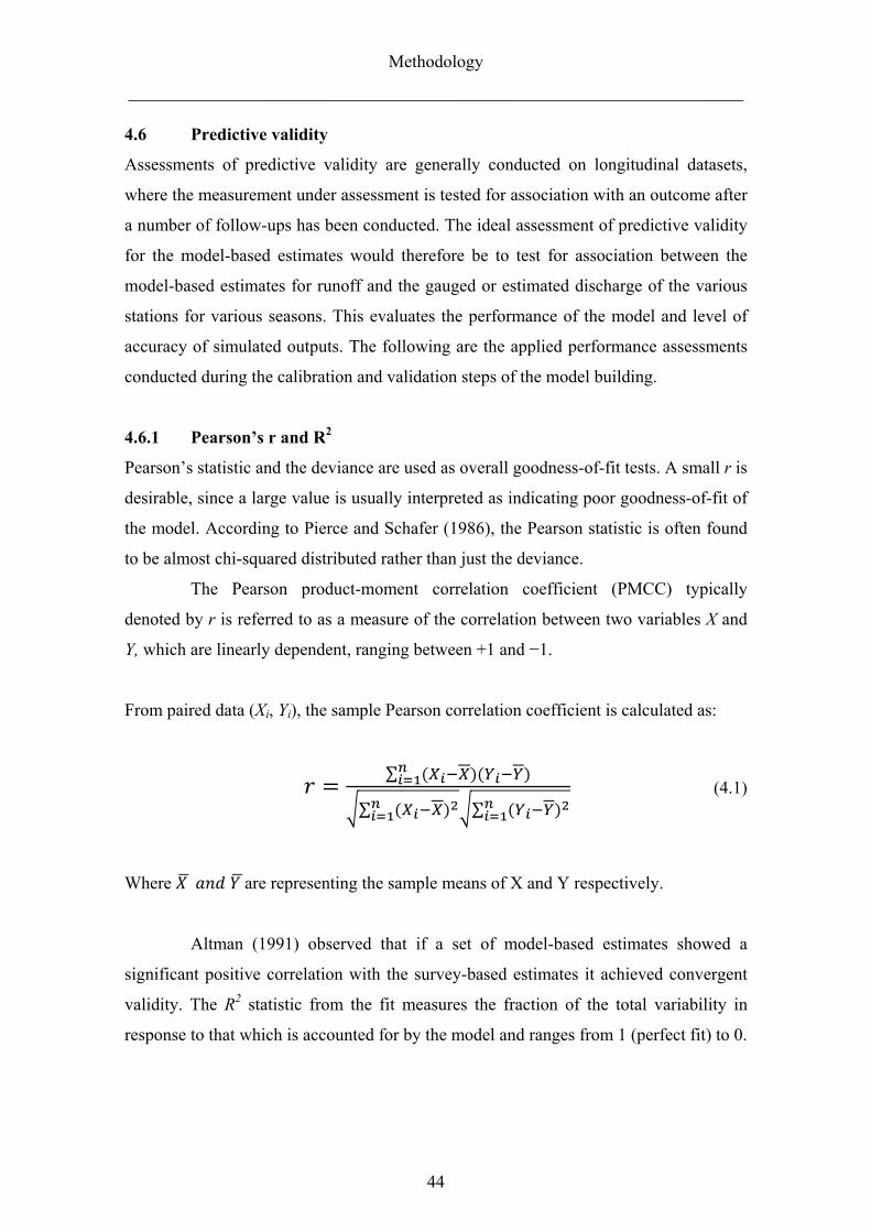
Methodology
______________________________________________________________________
44
4.6 Predictive validity
Assessments of predictive validity are generally conducted on longitudinal datasets,
where the measurement under assessment is tested for association with an outcome after
a number of follow-ups has been conducted. The ideal assessment of predictive validity
for the model-based estimates would therefore be to test for association between the
model-based estimates for runoff and the gauged or estimated discharge of the various
stations for various seasons. This evaluates the performance of the model and level of
accuracy of simulated outputs. The following are the applied performance assessments
conducted during the calibration and validation steps of the model building.
4.6.1 Pearson’s r and R2
Pearson’s statistic and the deviance are used as overall goodness-of-fit tests. A small r is
desirable, since a large value is usually interpreted as indicating poor goodness-of-fit of
the model. According to Pierce and Schafer (1986), the Pearson statistic is often found
to be almost chi-squared distributed rather than just the deviance.
The Pearson product-moment correlation coefficient (PMCC) typically
denoted by r is referred to as a measure of the correlation between two variables X and
Y, which are linearly dependent, ranging between +1 and −1.
From paired data (Xi, Yi), the sample Pearson correlation coefficient is calculated as:
∑
∑ ∑ (4.1)
Where are representing the sample means of X and Y respectively.
Altman (1991) observed that if a set of model-based estimates showed a
significant positive correlation with the survey-based estimates it achieved convergent
validity. The R2 statistic from the fit measures the fraction of the total variability in
response to that which is accounted for by the model and ranges from 1 (perfect fit) to 0.
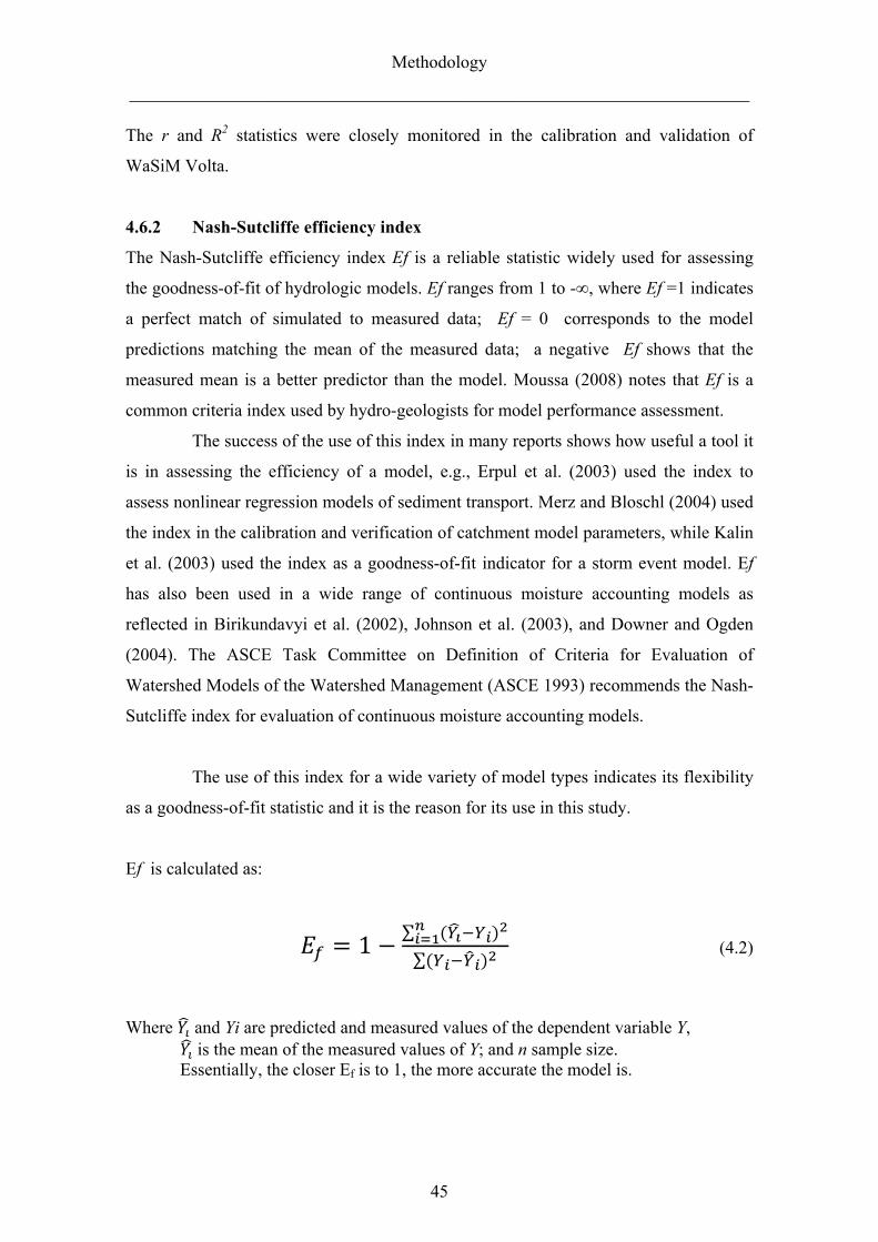
Methodology
______________________________________________________________________
45
The r and R2 statistics were closely monitored in the calibration and validation of
WaSiM Volta.
4.6.2 Nash-Sutcliffe efficiency index
The Nash-Sutcliffe efficiency index Ef is a reliable statistic widely used for assessing
the goodness-of-fit of hydrologic models. Ef ranges from 1 to -∞, where Ef =1 indicates
a perfect match of simulated to measured data; Ef = 0 corresponds to the model
predictions matching the mean of the measured data; a negative Ef shows that the
measured mean is a better predictor than the model. Moussa (2008) notes that Ef is a
common criteria index used by hydro-geologists for model performance assessment.
The success of the use of this index in many reports shows how useful a tool it
is in assessing the efficiency of a model, e.g., Erpul et al. (2003) used the index to
assess nonlinear regression models of sediment transport. Merz and Bloschl (2004) used
the index in the calibration and verification of catchment model parameters, while Kalin
et al. (2003) used the index as a goodness-of-fit indicator for a storm event model. Ef
has also been used in a wide range of continuous moisture accounting models as
reflected in Birikundavyi et al. (2002), Johnson et al. (2003), and Downer and Ogden
(2004). The ASCE Task Committee on Definition of Criteria for Evaluation of
Watershed Models of the Watershed Management (ASCE 1993) recommends the Nash-
Sutcliffe index for evaluation of continuous moisture accounting models.
The use of this index for a wide variety of model types indicates its flexibility
as a goodness-of-fit statistic and it is the reason for its use in this study.
Ef is calculated as:
1∑
∑ (4.2)
Where and Yi are predicted and measured values of the dependent variable Y, is the mean of the measured values of Y; and n sample size.
Essentially, the closer Ef is to 1, the more accurate the model is.
Methodology
______________________________________________________________________
46
4.6.3 Index of Agreement (d)
The Index of Agreement (d) is the evaluation of the agreement between the estimated
and observed runoff (Legates and McCabe, 1999; Willmott, 1984; and Willmott, 1981).
Recent successes in the use of (d) in hydrological modeling include Obuobie (2008),
Hiepe and Diekkrüger (2007), Chekol (2006) among others.
Willmott developed the index of agreement to overcome the insensitivity of
correlation-based measurements that were based on differences in sampled means and
variances of the observed and model-simulated outputs (Willmott, 1981 and 1984):
1.0∑
∑ (4.3)
where Oi is the observed data; Pi is the model-simulated values of Oi, is the mean of O; and n is the number of data O.
4.6.4 Mass balance error
The minimization of the errors in the mass balance is considered the most important
objective in calibration after the water balance is fairly correct. This is derived from the
fact that the processes within the unsaturated zone and evapotranspiration are
considered the core of the model, and the processes are responsible for keeping the mass
balance as realistic as possible. If good estimates are obtained for the parameters of
infiltration process (unsaturated zone), it is very likely that good estimates for runoff
starting time and good matches between simulated and observed surface discharge may
also be obtained (David et al., 1991).
4.7 Drought analysis in the Volta Basin
Evaluating future watershed changes is more difficult than the evaluation of changes
that have already taken place because of the non-stationary nature of some input data
such as land use/land cover. Satisfactory simulation of the water resources of the Volta
Methodology
______________________________________________________________________
47
meteorological, soil-moisture, and hydrological droughts. The different types of
droughts are linked (Figure 4.5) to each other with each type of drought referring to a
specific type of water deficit in a specific part of the hydrological cycle. A
meteorological drought is said to occur when precipitation is less than normal. Soil
moisture droughts and hydrological droughts are usually characterized by low soil water
content and low stream flows and usually occur after a meteorological drought. For the
development of soil moisture droughts, precipitation deficit coupled with high
evapotranspiration are the two most important factors. Low stream flows usually linked
to hydrological drought are common in the Volta Basin and can be linked to the
development of other types of droughts.
For this study, meteorological inputs for the past were obtained from the GVP.
For the simulations, the calibrated model generated inputs using the Mesoscale
Meteorological Model version 5 (MM5) adopted for the Volta Basin by the GVP, based
on the IS92a–f greenhouse gas emissions scenarios (IPCC 2001). The used REMO
model outputs were adopted by GLOWA IMPETUS project based on the IPCC climate
assemble models A1B and B1. The future time slice of 2030 to 2039 was compared
with time slices of the past and present climates of 1961-1970 and 1991-2000,
respectively, for the evaluation of changes with MM5 and 1961-2000 and 2001-2050
with REMO.
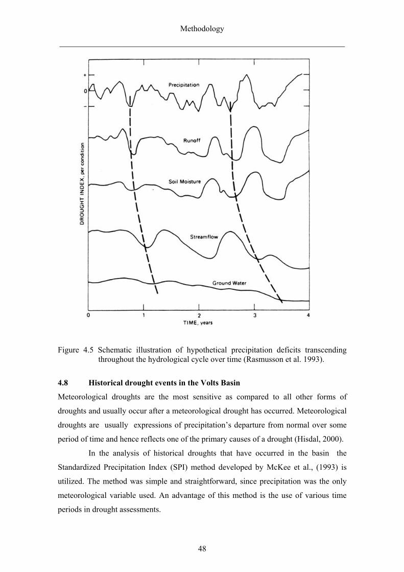
Methodology
______________________________________________________________________
48
Figure 4.5 Schematic illustration of hypothetical precipitation deficits transcending throughout the hydrological cycle over time (Rasmusson et al. 1993).
4.8 Historical drought events in the Volts Basin
Meteorological droughts are the most sensitive as compared to all other forms of
droughts and usually occur after a meteorological drought has occurred. Meteorological
droughts are usually expressions of precipitation’s departure from normal over some
period of time and hence reflects one of the primary causes of a drought (Hisdal, 2000).
In the analysis of historical droughts that have occurred in the basin the
Standardized Precipitation Index (SPI) method developed by McKee et al., (1993) is
utilized. The method was simple and straightforward, since precipitation was the only
meteorological variable used. An advantage of this method is the use of various time
periods in drought assessments.
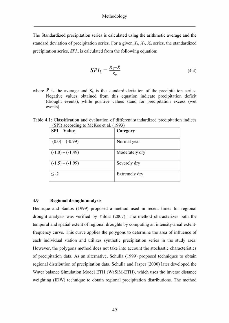
Methodology
______________________________________________________________________
49
The Standardized precipitation series is calculated using the arithmetic average and the
standard deviation of precipitation series. For a given X1, X2, Xn series, the standardized
precipitation series, SPIi, is calculated from the following equation:
(4.4)
where is the average and Sx is the standard deviation of the precipitation series. Negative values obtained from this equation indicate precipitation deficit (drought events), while positive values stand for precipitation excess (wet events).
Table 4.1: Classification and evaluation of different standardized precipitation indices (SPI) according to McKee et al. (1993)
SPI Value
Category
(0.0) – (-0.99)
Normal year
(-1.0) – (-1.49) Moderately dry
(-1.5) – (-1.99) Severely dry
≤ -2
Extremely dry
4.9 Regional drought analysis
Henrique and Santos (1999) proposed a method used in recent times for regional
drought analysis was verified by Yildiz (2007). The method characterizes both the
temporal and spatial extent of regional droughts by computing an intensity-areal extent-
frequency curve. This curve applies the polygons to determine the area of influence of
each individual station and utilizes synthetic precipitation series in the study area.
However, the polygons method does not take into account the stochastic characteristics
of precipitation data. As an alternative, Schulla (1999) proposed techniques to obtain
regional distribution of precipitation data. Schulla and Jasper (2000) later developed the
Water balance Simulation Model ETH (WaSiM-ETH), which uses the inverse distance
weighting (IDW) technique to obtain regional precipitation distributions. The method
Methodology
______________________________________________________________________
50
used in this study was used by Jung (2006) to evaluate runoff, evapotranspiration and
soil moisture dependency to climate change for the total catchment of the Volta River
basin. With the use of drought intensity-areal extent-frequency curves for a region
Henrique and Santos (1999) determined intensity, areal extent and return periods of
severe drought events. Similarly, in this study, a regional drought analysis was
performed for the Volta Basin using drought intensity, areal extent and frequency with
the method proposed by McKee et al. (1993) and Jung (2006).Annual drought intensity
values at each station were first obtained from the annual SPI time series over the whole
period of 1961-2005.
For this purpose, in a given year, SPI values of evenly spaced stations over the
basin were added together to obtain the total SPI intensities. Then the regional
distributions of annual drought intensities from 52 stations (Appendix I) were obtained
using the IDW method. Finally, percent areal distributions of drought intensities for
selected threshold levels (e.g., -1.0, -1.5, etc.) were calculated and a frequency analysis
of percent areal distributions was performed to determine return periods of drought
intensities.
Hydrological model WaSiM-ETH
______________________________________________________________________
51
5 HYDROLOGICAL MODEL WASIM-ETH
5.1 Introduction
WaSiM-ETH is a water balance simulation model and was first developed at the
Technical University of Zürich (ETH) (Schulla, 1997). It was later extended to combine
a 1-D unsaturated zone model based on the Richards equation with a watershed run-off
model by Schulla and Jasper (2000). Until recently, the hydrological model WaSiM has
not been used in a catchment of the size of the Volta Basin, or in a semi-arid
environment such as West Africa. WaSiM-ETH is popular in Europe and has been
applied in Germany and Switzerland in several researches, often to mountainous
watersheds (e.g., Schulla, (1997); Krause, (2003); Stadler, (2002) cited in Jung (2006)).
Within the GLOWA-Volta research project, WaSiM has been applied on three different
scales within the Volta Basin. the Atankwidi Basin covering an area of 275 km², the
White Volta catchment of 34,000 km², and the entire Volta Basin of 400,000 km²
(Martin, 2005; Wagner, 2008; Jung, 2006).
5.2 WaSiM Concept
WaSiM is a deterministic hydrological model with a modular structure. The open source
code is written in C+ consisting of three major components 1) the pre-processor
TANALYS (Topographical ANALYSis), which calculates basin boundaries, stream
network and flow times using the topographical information. This is used for processing
spatial raster data into the required input format for WaSiM model runs 2) The spatial
interpolation of meteorological input data and calculation of potential
evapotranspiration, and 3) flow dynamics in relation to water budget modeling.
The water budget simulation section of WaSiM comprises a chain of modules
that combine both the physical and empirical descriptions of water flow. Depending on
desired outputs and conditions of the area of interest, modules can be activated or
deactivated to reduce model run time and computer resources, The glacier and snow
modules were deactivated for this research because the area of interest (Volta Basin) is
in the tropics and has neither snow nor glaciers.
Hydrological model WaSiM-ETH
______________________________________________________________________
52
5.3 Data requirements and processing in WaSiM
The meteorological input data required are precipitation, temperature, relative humidity,
wind velocity, global radiation, and sunshine duration. Radiation and sunshine duration
are used alternatively. Of these input variables, temperature and precipitation are most
sensitive (Jung, 2006). However, to run WaSiM needs all these required parameters.
WaSiM employs a variety of methods of interpolation from gauged stationed data to a
regular grid. The methods available for interpolation are:
1) Inverse Distance Weighting (IDW): This interpolation method uses all available
station data within a specified search radius and performs a distance weighting
based on an assigned weighting.
2) Regression: In mountainous catchments, e.g., the mountainous landscape of
Switzerland, this mode of interpolation could be very important for variables
such as temperature and wind speed, which generally have a stronger
dependence on altitude than on horizontal positioning for such topography.
3) Regression and IDW: This method combines both altitude dependant regression
and IDW. Where using input variables from areas that are horizontally and
vertically correlated this method is useful for improving the temporal and spatial
resolutions of the interpolation.
4) Thiessen: This method is similar to IDW, but only considers the influence of the
station nearest to a certain grid point by drawing polygons around neighboring
stations and interpolating using the midpoint concept.
5) Bilinear interpolation: This is a method suitable for organized stations that are
equidistant, e.g., gridded input data are almost equidistant, hence the method of
bilinear interpolation is less time consuming and most effective.
5.3.1 Temporal data
Rainfall measurements are prone to errors partly from the method of collection and
largely due to human error. WaSiM in one of its steps of inputting the precipitation data,
usually termed “precipitation correction” within the control file, automatically makes
corrections to the precipitation data. These corrections are performed to counter the
Hydrological model WaSiM-ETH
______________________________________________________________________
53
errors induced by wind measurement. However, for simulated climate inputs, this
function is not required.
Radiation and temperature are usually topographically dependent and thus
require some adjustment. These adjustments are to compensate for shading effects due
to topography in mountainous regions. Sensible heat flux and temperature depend
strongly on incoming radiation. With the use of the DEM, incorporating the influence of
the topographical data using methods after Oke (1987) cited in Jung (2006), the needed
modifications are performed on the temperature and radiation inputs within the model.
Due to the flatness of the topography of the Volta Basin, the IDW
interpolation was used for the interpolation of the obtained station data in the calibration
and validation runs. For the future model runs when data from simulated climate models
were used, the bilinear interpolation method was satisfactory for the efficiency of
computer resources.
5.3.2 Spatial data
Hydrogeology
The hydrogeological inputs were largely from Martin and van de Giesen (2005) and
Jung (2006). Based on Jung (2006), parameterization of the geology of the basin was
carried out using various hydrogeological maps with additional information collected
from Ghana and Burkina Faso. Because data from other countries were not readily
available, extrapolation to the regions outside the Ghana and Burkina Faso boundaries
within the basin became necessary. Hydro-geological units, horizontal hydraulic
conductivities, storage coefficient and aquifer thicknesses were acquired from previous
research conducted by Jung (2006). Literature values were used for parameters that
were not location specific.
DEM
The digital elevation model (DEM) derived from the Shuttle Radar Topography Mission
(SRTM) subset at 90m resolution provided by the GVP (Figure 5.1) was used in the
topographical analysis (TANALYS) to derive exposition, slope, flow net structure, flow
directions, flow times, and sub-catchment boundaries based on gauging points.
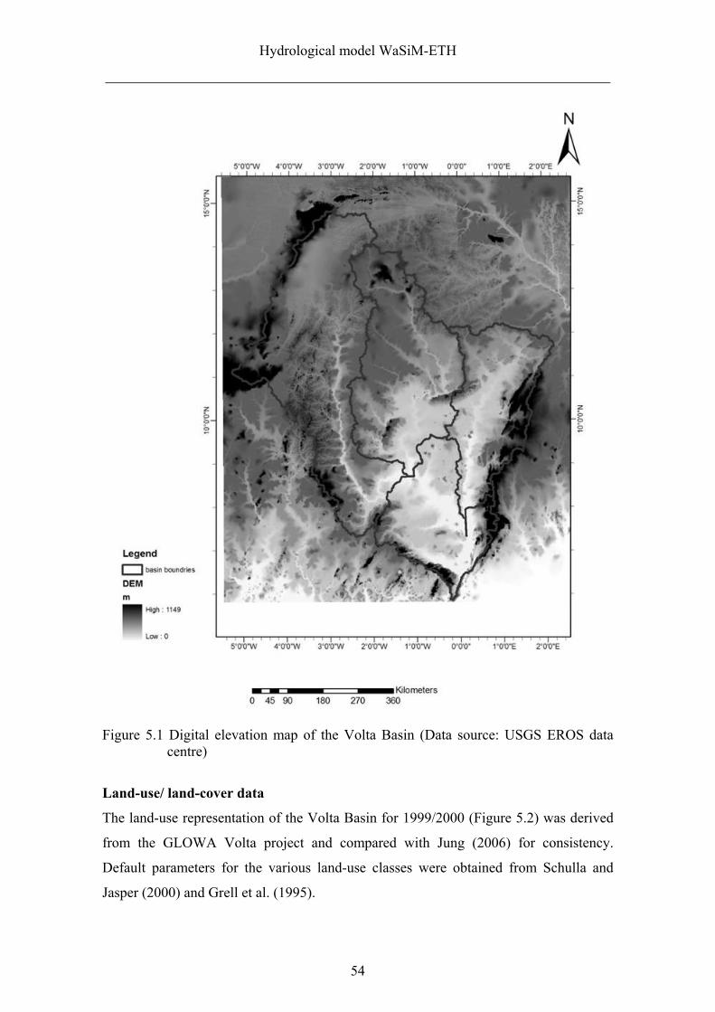
Hydrological model WaSiM-ETH
______________________________________________________________________
54
Figure 5.1 Digital elevation map of the Volta Basin (Data source: USGS EROS data centre)
Land-use/ land-cover data
The land-use representation of the Volta Basin for 1999/2000 (Figure 5.2) was derived
from the GLOWA Volta project and compared with Jung (2006) for consistency.
Default parameters for the various land-use classes were obtained from Schulla and
Jasper (2000) and Grell et al. (1995).
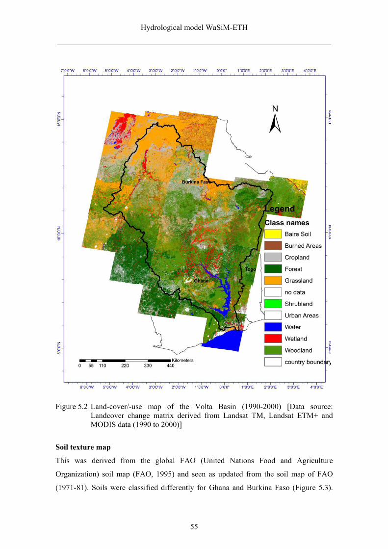
Hydrological model WaSiM-ETH
______________________________________________________________________
55
Figure 5.2 Land-cover/-use map of the Volta Basin (1990-2000) [Data source: Landcover change matrix derived from Landsat TM, Landsat ETM+ and MODIS data (1990 to 2000)]
Soil texture map
This was derived from the global FAO (United Nations Food and Agriculture
Organization) soil map (FAO, 1995) and seen as updated from the soil map of FAO
(1971-81). Soils were classified differently for Ghana and Burkina Faso (Figure 5.3).
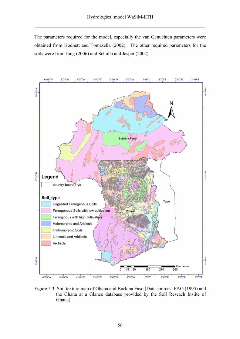
Hydrological model WaSiM-ETH
______________________________________________________________________
56
The parameters required for the model, especially the van Genuchten parameters were
obtained from Hodnett and Tomasella (2002). The other required parameters for the
soils were from Jung (2006) and Schulla and Jasper (2002).
Figure 5.3: Soil texture map of Ghana and Burkina Faso (Data sources: FAO (1995) and
the Ghana at a Glance database provided by the Soil Reseach Instite of Ghana)
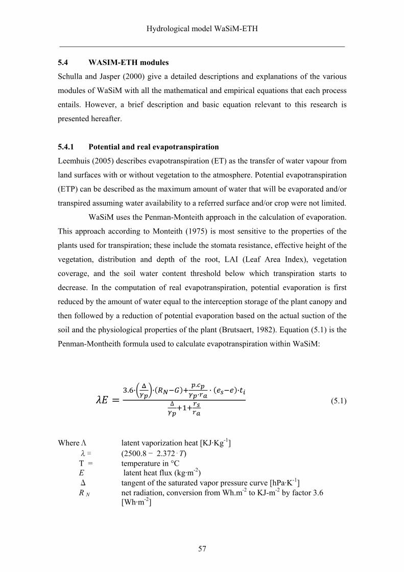
Hydrological model WaSiM-ETH
______________________________________________________________________
57
5.4 WASIM-ETH modules
Schulla and Jasper (2000) give a detailed descriptions and explanations of the various
modules of WaSiM with all the mathematical and empirical equations that each process
entails. However, a brief description and basic equation relevant to this research is
presented hereafter.
5.4.1 Potential and real evapotranspiration
Leemhuis (2005) describes evapotranspiration (ET) as the transfer of water vapour from
land surfaces with or without vegetation to the atmosphere. Potential evapotranspiration
(ETP) can be described as the maximum amount of water that will be evaporated and/or
transpired assuming water availability to a referred surface and/or crop were not limited.
WaSiM uses the Penman-Monteith approach in the calculation of evaporation.
This approach according to Monteith (1975) is most sensitive to the properties of the
plants used for transpiration; these include the stomata resistance, effective height of the
vegetation, distribution and depth of the root, LAI (Leaf Area Index), vegetation
coverage, and the soil water content threshold below which transpiration starts to
decrease. In the computation of real evapotranspiration, potential evaporation is first
reduced by the amount of water equal to the interception storage of the plant canopy and
then followed by a reduction of potential evaporation based on the actual suction of the
soil and the physiological properties of the plant (Brutsaert, 1982). Equation (5.1) is the
Penman-Montheith formula used to calculate evapotranspiration within WaSiM:
. · ·.
· · ·
∆ (5.1)
WhereΛ latent vaporization heat [KJ·Kg-1] λ= (2500.8 − 2.372⋅T) T = temperature in °C E latent heat flux (kg·m-2) Δ tangent of the saturated vapor pressure curve [hPa·K-1] R N net radiation, conversion from Wh.m-2 to KJ-m-2 by factor 3.6 [Wh·m-2]
Hydrological model WaSiM-ETH
______________________________________________________________________
58
G soil heat flux [Wh·m-2] p density of dry air (kg·m³) p (RL ⋅T) (at 0°C and 1013.25 hPa: p
=1.26) c p specific heat capacity of dry air (KJ·(Kg·K)-1) at constant pressure c p = 1.005 e s saturation vapor pressure at temperature T [hPa] e actual vapour pressure (observed) (hPa) t i number of seconds within a time step γ psychrometric constant [hPa·K-1] r s bulk-surface resistance [s·m-1] r a bulk-aerodynamic resistance [s·m-1]
5.4.2 Interception
Interception is that part of precipitation caught up by canopy formed by the vegetation
above the ground. For WaSiM, the simple bucket approach is used for the computation
of interception storage, which is dependent on the total leave coverage (a factor of LAI)
and the maximum height of the water layer on the vegetation. The underlying equation
(5.2) after Schulla (1997) has varied conditions for too dry or wet soil:
· · 1 · (5.2)
Where SI max maximum interception storage capacity [mm] v degree of vegetation coverage [m2/m-2] LAI leaf area index [m2/m-2] h SI maximum height of water [mm]
According to the developers of the model, the extraction of water out of the interception
storage by evaporation is assumed to be at a potential rate. If there is a sufficient amount
of water in the storage, the storage content is reduced by the potential evaporation, and
no evaporation water will be taken from the soil. If the storage content is smaller than
the potential evaporation rate, the remaining rate will be taken from the soil on
condition that the soil is not too dry or too wet. In that light, interception evaporation
will be:
EI =ETP (for SI ≥ ETP in mm), ETR = 0 and EI = SI (for SI < ETP in mm), ETR = ETP –SI
where EI the interception evaporation [mm] ETR remaining evaporation from soil and vegetation SI content of the interception storage [mm]
Hydrological model WaSiM-ETH
______________________________________________________________________
59
5.4.3 Snow module
WaSiM also includes a snow module, which simulates melting and accumulation of
snow and their contributions to the water balance. However, in this study this module
was useless because of the geographical location of the Volta Basin in the tropics and
therefore was disabled.
5.4.4 Infiltration and the unsaturated zone module
In the modified Green and Ampt approach (1911), excess infiltration feeds directly to
runoff, and the amount of infiltrating water serves as an upper boundary condition in the
unsaturated zone module. In WaSiM release-2 (version 7.10.3) used in this research, the
downward movement of water through the soil after Green and Ampt (1911) stems from
the principle that, when saturation is reached or in situations when precipitation
intensity exceeds infiltration capacities, almost all the excess precipitation is channeled
into direct runoff. This module is hampered when potential macro-pore fluxes are not
considered. This restriction for the Volta Basin affected the performance of the
calibration and validation of the model. One major handicap was the use of daily
precipitation values for simulations, which assumes a mean value over 24 hrs. A better
resolution of at least a3-hr time step is desirable. The following equation is for the
calculation of infiltration:
If
· ⁄ (5.3)
Where t S saturation deficit from the beginning of the time step [h] l S saturation depth [mm]
n a fillable porosity (na = θS − θ) [-]
ψf suction of the wetting front ( a ≈ 1000n ) [mm] PI precipitation intensity [mm·h-1] K S saturated hydraulic conductivity [mm·h-1]
Hydrological model WaSiM-ETH
______________________________________________________________________
60
The water infiltrated until time Fs is calculated as:
· · (5.4)
Hence, using the formula after Peschke (1989), the accumulated infiltration
after saturation has been reached due to peculation for one time step is determined as:
(5.5)
Where and 2. .
Within the unsaturated zone, calculation of vertical movement of water in soil
assumes this zone as one-dimensional so that no exchange of water between
neighboring cells takes place.
Each cell is divided into layers of uniform thickness as specified in the soil
module. Percolation and capillary rise according to the soil properties are simulated
with corresponding vertical moisture profiles and fluxes. The van Genuchten equation is
used to account for the hydraulic conductivity with decreasing water content (van
Genuchten, 1980). The water release curve of soils is a function of the saturated (Өs)
and residual (Өr) soil water content, the soil matrix potential ψ and the parameters α and
n with the premise that hydraulic head and conductivities depend on the van Genuchten
principles (1980).
| (5.6)
Whereθ actual water content [-]
ψ suction [hPa] θr residual water content at k(θ)= 0 [-] θs saturation water content [-] α, n empirical parameter (m=1-1/n) [-]
Hydrological model WaSiM-ETH
______________________________________________________________________
61
Due to flow retention, linear storage approaches are applied to interflow and direct
runoff, which requires the calibration of the recession constants KD and KI. Similarily,
the runoff at time t, (Qt) is a result of the runoff component at the initial time t0, (Qt0)
and the corresponding recession constants K as given in the relation:
· ∆
(5.7)
with change in time ∆
Bare soils on top of the soil profiles of the unsaturated zones are responsible for
evaporation, while plants are responsible for uptake of water from other soil layers for
transpiration, depending on the properties of the plant and the availability of moisture.
Interflow is generated between soil layers and relies upon the suction and the
drainage density of the soil. Groundwater recharge is also calculated as the balance of
inflows and outflows to the total layers in which the groundwater table resides.
The van Genuchten equation (5.6) is often used to determine unsaturated
hydraulic conductivities.
5.4.5 Run-off routing
The run-off is that component that includes direct run-off, interflow and base flows
assuming the groundwater module was inactive. The generated runoff in each cell is
directed to the outlet of a basin with respect to flow times that are calculated by the pre-
processor TANALYS for the entire catchment considering the distances to specific
routed outlets (Figure 5.4). The different flow velocities for the different water levels in
the channels are calculated using the kinetic wave approach and a simple linear storage
approach. Thereafter, direct runoff and interflow are simulated. These flow times are
calculated using the Manning-Strickler equation (Maidment, 1993). It is possible to
simulate other processes within the catchments such as irrigation, artificial abstractions
and regulated reservoirs.
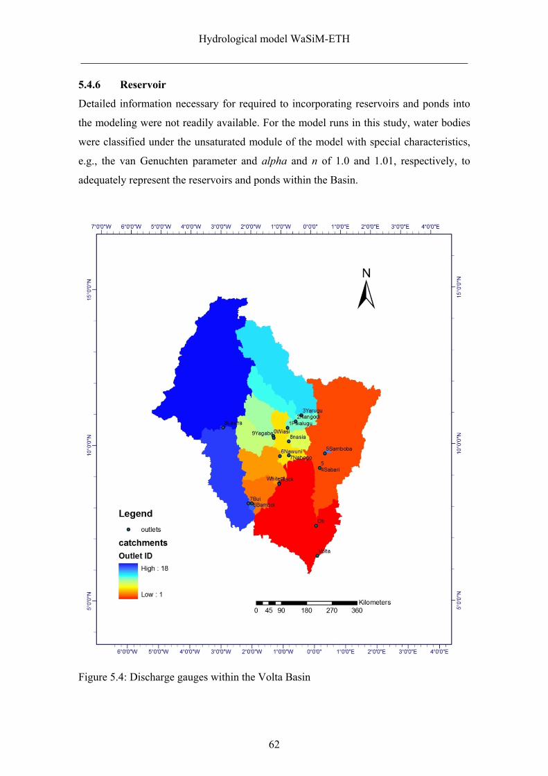
Hydrological model WaSiM-ETH
______________________________________________________________________
62
5.4.6 Reservoir
Detailed information necessary for required to incorporating reservoirs and ponds into
the modeling were not readily available. For the model runs in this study, water bodies
were classified under the unsaturated module of the model with special characteristics,
e.g., the van Genuchten parameter and alpha and n of 1.0 and 1.01, respectively, to
adequately represent the reservoirs and ponds within the Basin.
Figure 5.4: Discharge gauges within the Volta Basin
Hydrological model WaSiM-ETH
______________________________________________________________________
63
5.5 Calibration of WaSiM-ETH
Calibrating WaSiM for the Volta Basin requires adequate information in input
parameters, especially climatic and hydrological (Table 5.1). This is essential for the
Volta Basin according to Jung (2006), because this region lacks the necessary
infrastructure, thus making this step the most important in the process of building up an
efficient and reliable model. A short history of the basin and reports such as Jung (2006)
and Wagner (2008) reveal that the natural flow regimes within the basin have been
altered since the early 1970s due to the construction of dams and irrigation systems.
Hence the periods before the 1970 were most suitable for the calibration. However,
considering the availability of reliable data, the period 1968-1971 was selected as the
calibration period. The selected period has meteorological and hydrological observation
time series data with fewer gaps compared to other periods for the selected catchments.
A rough sensitivity analysis showed that the drainage density dr (an empirical scaling
parameter) responsible for linearly controlling the strength of interflow, and the
calibration of the recession constant Krec, the factor that controls the reduction of the
saturated hydraulic conductivity with depth, were the main drivers in the water balance.
The initialization condition of the groundwater level in a soil profile was set on default,
setting the initial level at 40 % of the assigned profile column.
5.6 Main calibration parameters
WaSiM was calibrated for selected watersheds within the basin that had observed
stream data available for the calibration periods and thereafter applied to other parts of
the basin for various simulations (Table 5.2).
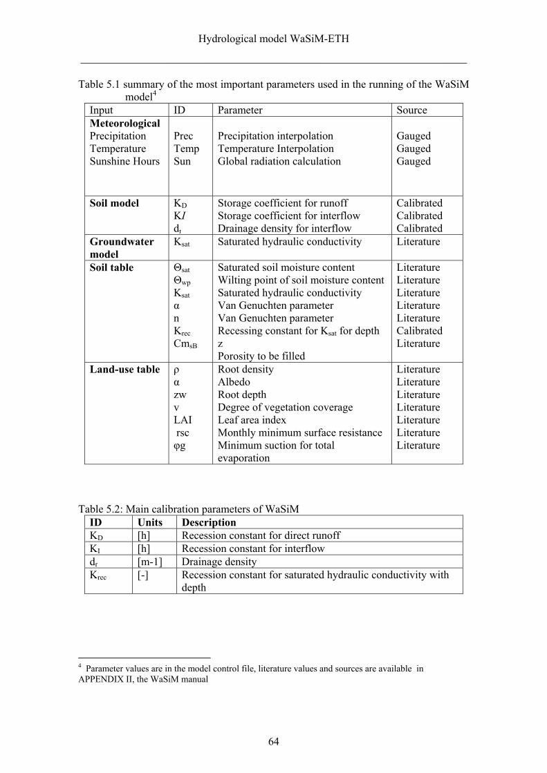
Hydrological model WaSiM-ETH
______________________________________________________________________
64
Table 5.1 summary of the most important parameters used in the running of the WaSiM model4
Input ID Parameter Source Meteorological Precipitation Temperature Sunshine Hours
Prec Temp Sun
Precipitation interpolation Temperature Interpolation Global radiation calculation
Gauged Gauged Gauged
Soil model
KD KI dr
Storage coefficient for runoff Storage coefficient for interflow Drainage density for interflow
Calibrated Calibrated Calibrated
Groundwater model
Ksat Saturated hydraulic conductivity Literature
Soil table
Θsat Θwp Ksat α n Krec CmsB
Saturated soil moisture content Wilting point of soil moisture content Saturated hydraulic conductivity Van Genuchten parameter Van Genuchten parameter Recessing constant for Ksat for depth z Porosity to be filled
Literature Literature Literature Literature Literature Calibrated Literature
Land-use table ρ α zw v LAI rsc φg
Root density Albedo Root depth Degree of vegetation coverage Leaf area index Monthly minimum surface resistance Minimum suction for total evaporation
Literature Literature Literature Literature Literature Literature Literature
Table 5.2: Main calibration parameters of WaSiM ID Units Description KD [h] Recession constant for direct runoff KI [h] Recession constant for interflow dr [m-1] Drainage density Krec [-] Recession constant for saturated hydraulic conductivity with
depth
4 Parameter values are in the model control file, literature values and sources are available in APPENDIX II, the WaSiM manual
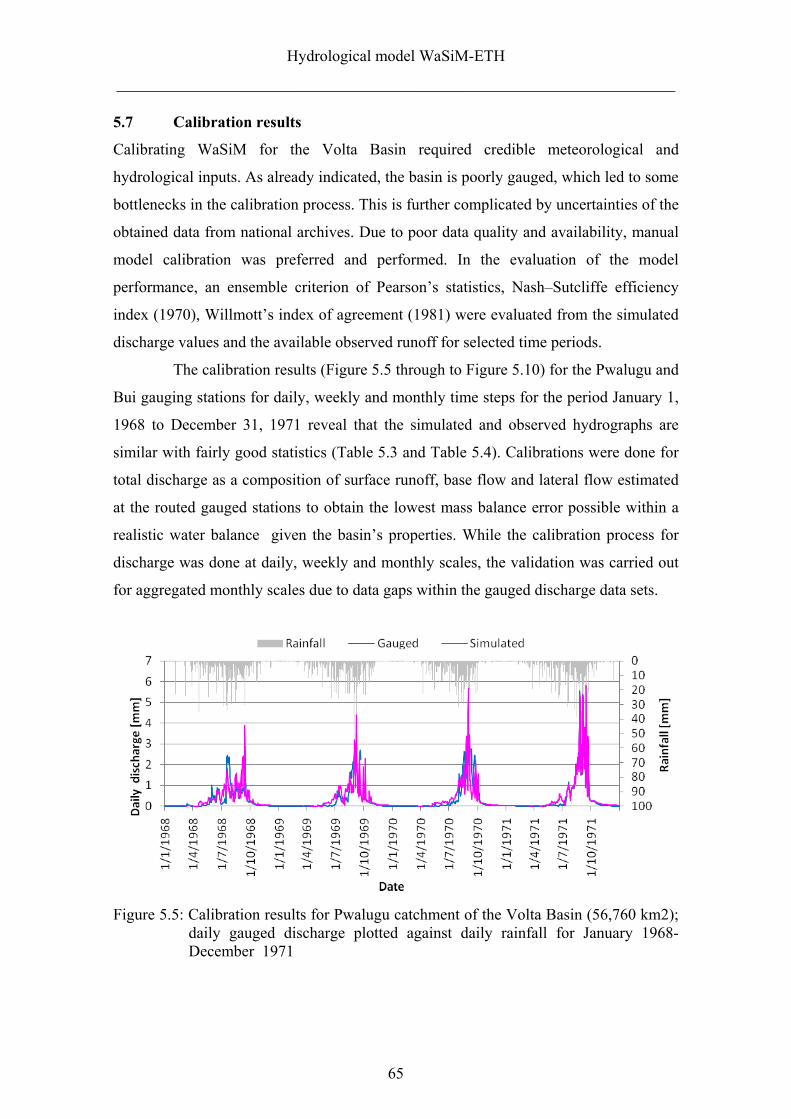
Hydrological model WaSiM-ETH
______________________________________________________________________
65
5.7 Calibration results
Calibrating WaSiM for the Volta Basin required credible meteorological and
hydrological inputs. As already indicated, the basin is poorly gauged, which led to some
bottlenecks in the calibration process. This is further complicated by uncertainties of the
obtained data from national archives. Due to poor data quality and availability, manual
model calibration was preferred and performed. In the evaluation of the model
performance, an ensemble criterion of Pearson’s statistics, Nash–Sutcliffe efficiency
index (1970), Willmott’s index of agreement (1981) were evaluated from the simulated
discharge values and the available observed runoff for selected time periods.
The calibration results (Figure 5.5 through to Figure 5.10) for the Pwalugu and
Bui gauging stations for daily, weekly and monthly time steps for the period January 1,
1968 to December 31, 1971 reveal that the simulated and observed hydrographs are
similar with fairly good statistics (Table 5.3 and Table 5.4). Calibrations were done for
total discharge as a composition of surface runoff, base flow and lateral flow estimated
at the routed gauged stations to obtain the lowest mass balance error possible within a
realistic water balance given the basin’s properties. While the calibration process for
discharge was done at daily, weekly and monthly scales, the validation was carried out
for aggregated monthly scales due to data gaps within the gauged discharge data sets.
Figure 5.5: Calibration results for Pwalugu catchment of the Volta Basin (56,760 km2); daily gauged discharge plotted against daily rainfall for January 1968- December 1971
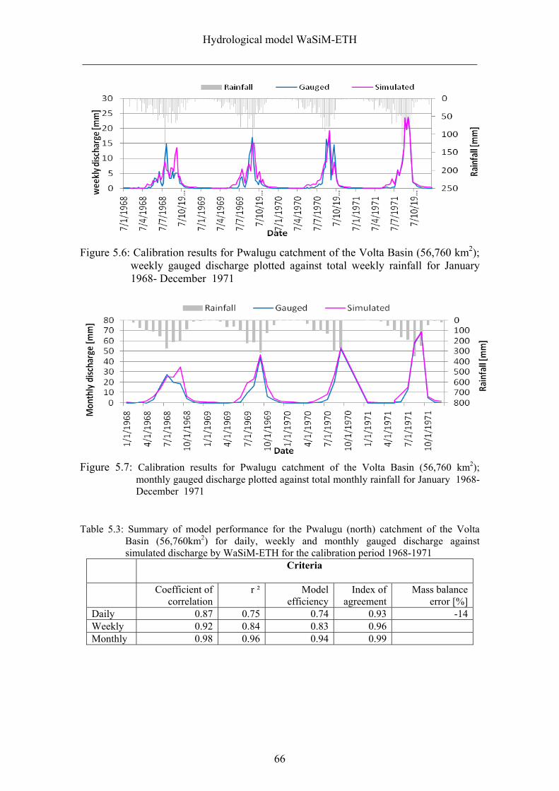
Hydrological model WaSiM-ETH
______________________________________________________________________
66
Figure 5.6: Calibration results for Pwalugu catchment of the Volta Basin (56,760 km2); weekly gauged discharge plotted against total weekly rainfall for January 1968- December 1971
Figure 5.7: Calibration results for Pwalugu catchment of the Volta Basin (56,760 km2); monthly gauged discharge plotted against total monthly rainfall for January 1968- December 1971
Table 5.3: Summary of model performance for the Pwalugu (north) catchment of the Volta
Basin (56,760km2) for daily, weekly and monthly gauged discharge against simulated discharge by WaSiM-ETH for the calibration period 1968-1971
Criteria
Coefficient of correlation
r ² Model efficiency
Index of agreement
Mass balance error [%]
Daily 0.87 0.75 0.74 0.93 -14Weekly 0.92 0.84 0.83 0.96Monthly 0.98 0.96 0.94 0.99
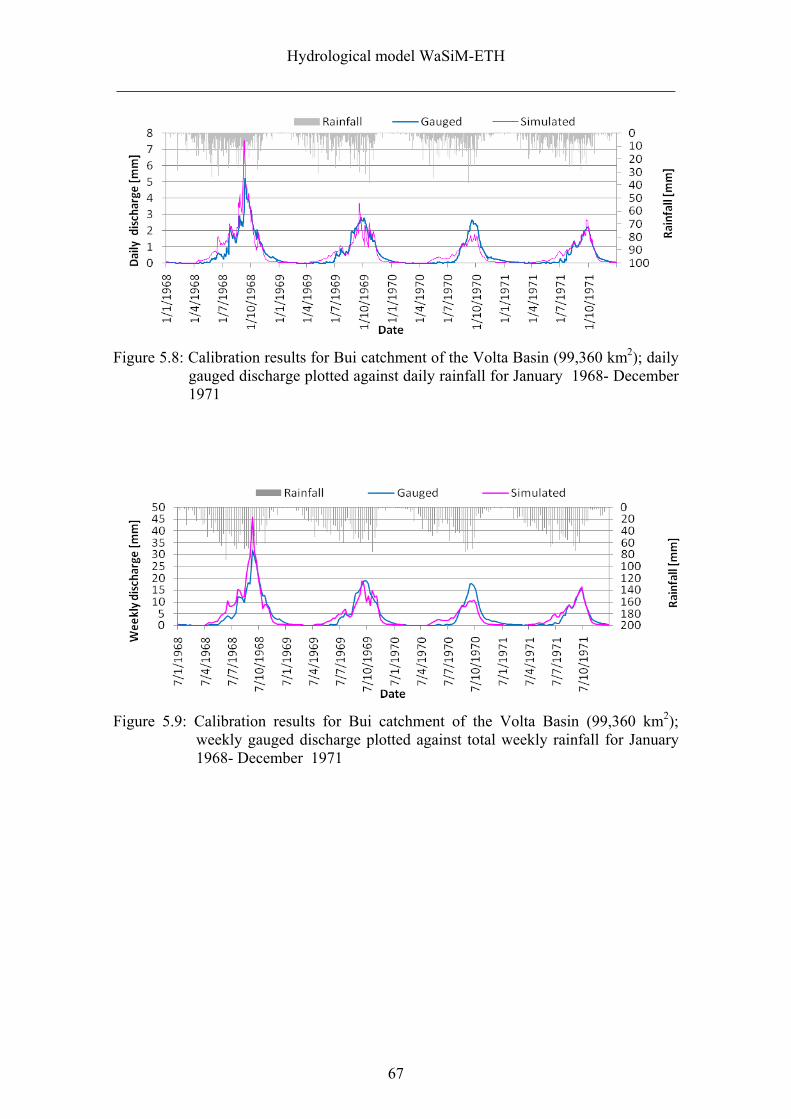
Hydrological model WaSiM-ETH
______________________________________________________________________
67
Figure 5.8: Calibration results for Bui catchment of the Volta Basin (99,360 km2); daily gauged discharge plotted against daily rainfall for January 1968- December 1971
Figure 5.9: Calibration results for Bui catchment of the Volta Basin (99,360 km2); weekly gauged discharge plotted against total weekly rainfall for January 1968- December 1971
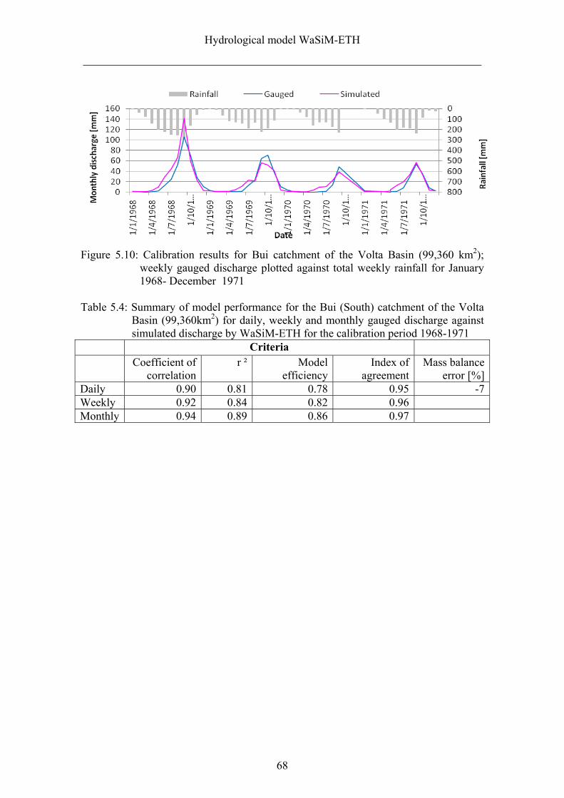
Hydrological model WaSiM-ETH
______________________________________________________________________
68
Figure 5.10: Calibration results for Bui catchment of the Volta Basin (99,360 km2); weekly gauged discharge plotted against total weekly rainfall for January 1968- December 1971
Table 5.4: Summary of model performance for the Bui (South) catchment of the Volta
Basin (99,360km2) for daily, weekly and monthly gauged discharge against simulated discharge by WaSiM-ETH for the calibration period 1968-1971
Criteria Coefficient of
correlation r ² Model
efficiencyIndex of
agreement Mass balance
error [%]Daily 0.90 0.81 0.78 0.95 -7Weekly 0.92 0.84 0.82 0.96 Monthly 0.94 0.89 0.86 0.97

Hyd
rolo
gica
l mod
el W
aSiM
-ET
H
___
____
____
____
____
____
____
____
____
____
____
____
____
____
____
____
____
___
69
Tab
le 5
.5:
Sum
mar
y of
sim
ulat
ed w
ater
bal
ance
for
the
Pw
alug
u (n
orth
) ca
tchm
ent
(56,
760k
m2 )
and
Bui
(so
uth)
cat
chm
ent
of t
he V
olta
B
asin
(99
,360
km2 )
for
the
cali
brat
ion
peri
od 1
968-
1971
C
atch
men
t P
wal
ugu
(nor
th)
Bui
(S
outh
) B
alan
ce te
rm
sim
ulat
ed
[mm
]pa
rt o
f pr
ecn5
(%)
aver
age
per
year
[m
m]
sim
ulat
ed
[mm
]pa
rt o
f pr
ecn
(%)
aver
age
per
year
[m
m]
Rai
nfal
l 48
2710
012
07
5631
100
1408
Tot
al d
isch
arge
52
511
131
909
1622
7S
urfa
ce f
low
10
62
26
274
569
Inte
r fl
ow
358
789
54
510
136
Bas
e fl
ow
621
16
912
23P
oten
tial
ev
apot
rans
pira
tion
11
184
232
2796
10
844
193
2711
Act
ual
evap
otra
nspi
rati
on
4081
8510
20
4585
8111
46
Bal
ance
cha
nge
221
555
13
72
34S
oil w
ater
con
tent
ch
ange
-2
24-5
-56
-139
-3-3
5
Bal
ance
err
or
-3-0
.1-0
.8
-3-0
.1-0
.7
5 Pre
cn =
per
cen
tage
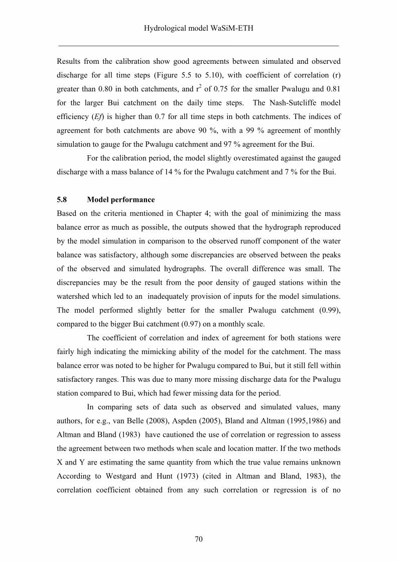
Hydrological model WaSiM-ETH
______________________________________________________________________
70
Results from the calibration show good agreements between simulated and observed
discharge for all time steps (Figure 5.5 to 5.10), with coefficient of correlation (r)
greater than 0.80 in both catchments, and r2 of 0.75 for the smaller Pwalugu and 0.81
for the larger Bui catchment on the daily time steps. The Nash-Sutcliffe model
efficiency (Ef) is higher than 0.7 for all time steps in both catchments. The indices of
agreement for both catchments are above 90 %, with a 99 % agreement of monthly
simulation to gauge for the Pwalugu catchment and 97 % agreement for the Bui.
For the calibration period, the model slightly overestimated against the gauged
discharge with a mass balance of 14 % for the Pwalugu catchment and 7 % for the Bui.
5.8 Model performance
Based on the criteria mentioned in Chapter 4; with the goal of minimizing the mass
balance error as much as possible, the outputs showed that the hydrograph reproduced
by the model simulation in comparison to the observed runoff component of the water
balance was satisfactory, although some discrepancies are observed between the peaks
of the observed and simulated hydrographs. The overall difference was small. The
discrepancies may be the result from the poor density of gauged stations within the
watershed which led to an inadequately provision of inputs for the model simulations.
The model performed slightly better for the smaller Pwalugu catchment (0.99),
compared to the bigger Bui catchment (0.97) on a monthly scale.
The coefficient of correlation and index of agreement for both stations were
fairly high indicating the mimicking ability of the model for the catchment. The mass
balance error was noted to be higher for Pwalugu compared to Bui, but it still fell within
satisfactory ranges. This was due to many more missing discharge data for the Pwalugu
station compared to Bui, which had fewer missing data for the period.
In comparing sets of data such as observed and simulated values, many
authors, for e.g., van Belle (2008), Aspden (2005), Bland and Altman (1995,1986) and
Altman and Bland (1983) have cautioned the use of correlation or regression to assess
the agreement between two methods when scale and location matter. If the two methods
X and Y are estimating the same quantity from which the true value remains unknown
According to Westgard and Hunt (1973) (cited in Altman and Bland, 1983), the
correlation coefficient obtained from any such correlation or regression is of no
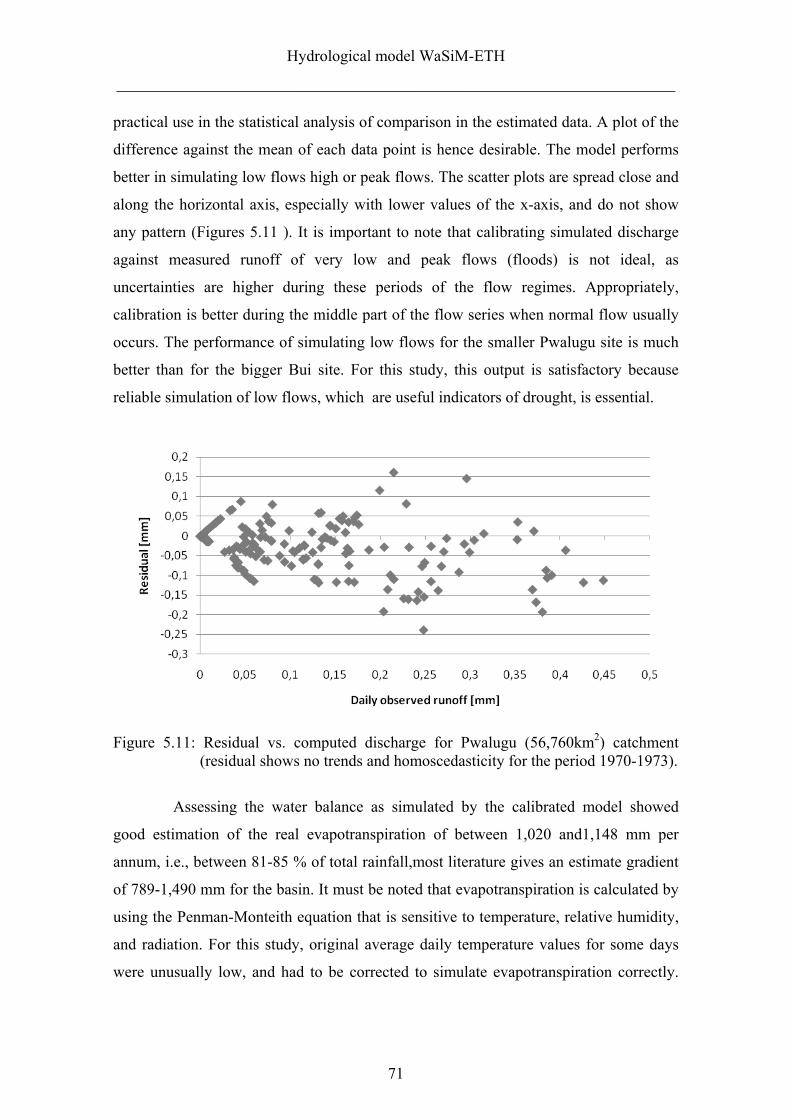
Hydrological model WaSiM-ETH
______________________________________________________________________
71
practical use in the statistical analysis of comparison in the estimated data. A plot of the
difference against the mean of each data point is hence desirable. The model performs
better in simulating low flows high or peak flows. The scatter plots are spread close and
along the horizontal axis, especially with lower values of the x-axis, and do not show
any pattern (Figures 5.11 ). It is important to note that calibrating simulated discharge
against measured runoff of very low and peak flows (floods) is not ideal, as
uncertainties are higher during these periods of the flow regimes. Appropriately,
calibration is better during the middle part of the flow series when normal flow usually
occurs. The performance of simulating low flows for the smaller Pwalugu site is much
better than for the bigger Bui site. For this study, this output is satisfactory because
reliable simulation of low flows, which are useful indicators of drought, is essential.
Figure 5.11: Residual vs. computed discharge for Pwalugu (56,760km2) catchment (residual shows no trends and homoscedasticity for the period 1970-1973).
Assessing the water balance as simulated by the calibrated model showed
good estimation of the real evapotranspiration of between 1,020 and1,148 mm per
annum, i.e., between 81-85 % of total rainfall,most literature gives an estimate gradient
of 789-1,490 mm for the basin. It must be noted that evapotranspiration is calculated by
using the Penman-Monteith equation that is sensitive to temperature, relative humidity,
and radiation. For this study, original average daily temperature values for some days
were unusually low, and had to be corrected to simulate evapotranspiration correctly.
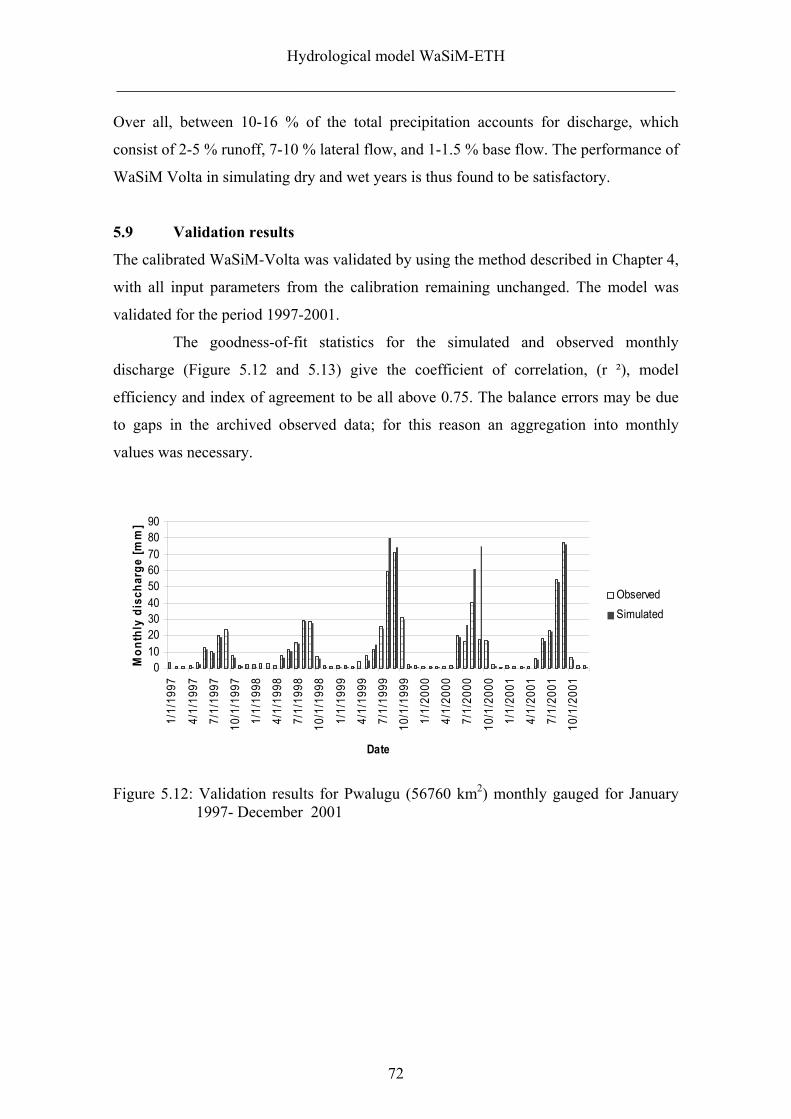
Hydrological model WaSiM-ETH
______________________________________________________________________
72
Over all, between 10-16 % of the total precipitation accounts for discharge, which
consist of 2-5 % runoff, 7-10 % lateral flow, and 1-1.5 % base flow. The performance of
WaSiM Volta in simulating dry and wet years is thus found to be satisfactory.
5.9 Validation results
The calibrated WaSiM-Volta was validated by using the method described in Chapter 4,
with all input parameters from the calibration remaining unchanged. The model was
validated for the period 1997-2001.
The goodness-of-fit statistics for the simulated and observed monthly
discharge (Figure 5.12 and 5.13) give the coefficient of correlation, (r ²), model
efficiency and index of agreement to be all above 0.75. The balance errors may be due
to gaps in the archived observed data; for this reason an aggregation into monthly
values was necessary.
0102030405060708090
1/1/
1997
4/1/
1997
7/1/
1997
10/1
/199
7
1/1/
1998
4/1/
1998
7/1/
1998
10/1
/199
8
1/1/
1999
4/1/
1999
7/1/
1999
10/1
/199
9
1/1/
2000
4/1/
2000
7/1/
2000
10/1
/200
0
1/1/
2001
4/1/
2001
7/1/
2001
10/1
/200
1
Date
Mo
nth
ly d
isch
arg
e [m
m]
Observed
Simulated
Figure 5.12: Validation results for Pwalugu (56760 km2) monthly gauged for January 1997- December 2001
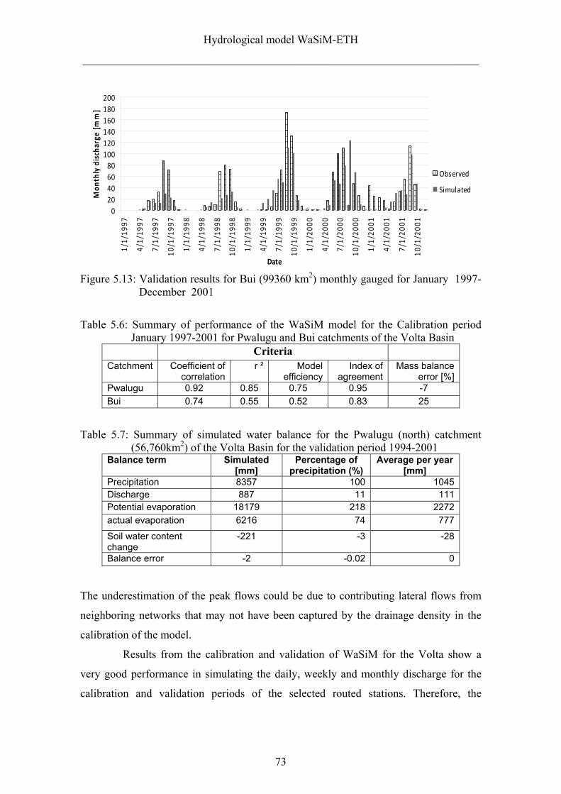
Hydrological model WaSiM-ETH
______________________________________________________________________
73
0
20
40
60
80
100
120
140
160
180
200
1/1
/1997
4/1
/1997
7/1
/1997
10/1
/1997
1/1
/1998
4/1
/1998
7/1
/1998
10/1
/1998
1/1
/1999
4/1
/1999
7/1
/1999
10/1
/1999
1/1
/2000
4/1
/2000
7/1
/2000
10/1
/2000
1/1
/2001
4/1
/2001
7/1
/2001
10/1
/2001
Date
Month
ly disch
arge
[mm]
Observed
Simulated
Figure 5.13: Validation results for Bui (99360 km2) monthly gauged for January 1997-
December 2001
Table 5.6: Summary of performance of the WaSiM model for the Calibration period
January 1997-2001 for Pwalugu and Bui catchments of the Volta Basin Criteria
Catchment Coefficient of correlation
r ² Model efficiency
Index of agreement
Mass balance error [%]
Pwalugu 0.92 0.85 0.75 0.95 -7
Bui 0.74 0.55 0.52 0.83 25
Table 5.7: Summary of simulated water balance for the Pwalugu (north) catchment (56,760km2) of the Volta Basin for the validation period 1994-2001
Balance term Simulated [mm]
Percentage of precipitation (%)
Average per year [mm]
Precipitation 8357 100 1045 Discharge 887 11 111 Potential evaporation 18179 218 2272
actual evaporation 6216 74 777
Soil water content change
-221 -3 -28
Balance error -2 -0.02 0
The underestimation of the peak flows could be due to contributing lateral flows from
neighboring networks that may not have been captured by the drainage density in the
calibration of the model.
Results from the calibration and validation of WaSiM for the Volta show a
very good performance in simulating the daily, weekly and monthly discharge for the
calibration and validation periods of the selected routed stations. Therefore, the
Hydrological model WaSiM-ETH
______________________________________________________________________
74
hydrological parameters adopted for the catchments and hence for the basin adequately
represent those of the basin and hence can mimic the hydrology of the Volta Basin for
further analysis.
5.10 Water Balance
Comparison of wet (1931–1969) and dry (1970– 1995) periods of the Volta Basin,
shows that on the whole, the ratio between direct runoff and base flow is 54 % to 46 %,
with a maximum during the wet years at 66 % and a sharp decline to 6 % in dry years .
According to Friesen et al. (2005), the decline of base flow is even more extreme when
short dry spells of 2-4 years of constantly low rain occur. These findings conformed to
results in the calibration and validation periods of this study (Table 5.6).
Table 5.8 Annual mean values of the water balance of the Pwalugu catchment of the Volta Basin of calibration (1967-1973) and validation (1994-2001)
1967-1973 1994-2001 Balance term average per
yearCV average
per year CV Literature
range Precipitation 1131 0.02 1045 0.09 910-1400a-g Total discharge 184 0.93 111 0.73 8-22%a-g Lateral flow 127 31 1-6%f Surface runoff 39 73* Base flow 19 7* 3-5%* Potential Evapotranspiration 1759 0.03 2272 0.25 1340-
2275b,e Actual Evapotranspiration 761 0.33 777 0.32 789-1490b,e Soil water Content change -17 -28 * Usually combined as reported as base flow or lateral flow. (a): Acheampong (1996); (b)Andreini et al. (2000); (c) Shahin (2002); (d): Martin (2005); (e): Friesen et al. (2005); (f): Darko and Krasn, (g) Obuobie, 2008
During the latter years of validation, evapotranspiration was 5 % higher (73
%) than in the calibration period . The annual discharge for the calibration period was
estimated at 16 % of the annual precipitation against the 11 % during the validation
period.
Base flow and lateral flow constituted 5 % during the calibration period and 3
% for the validation periods. The dynamics as simulated by WaSiM Volta are coherent
with the general trend in most parts of the Volta Basin. As already stated in this study,
over 80 % of the basin show a mono modal rainfall pattern, with a 6 to 7 months rainy
season (Figure 5.14) starting in April-May and peaking in August.
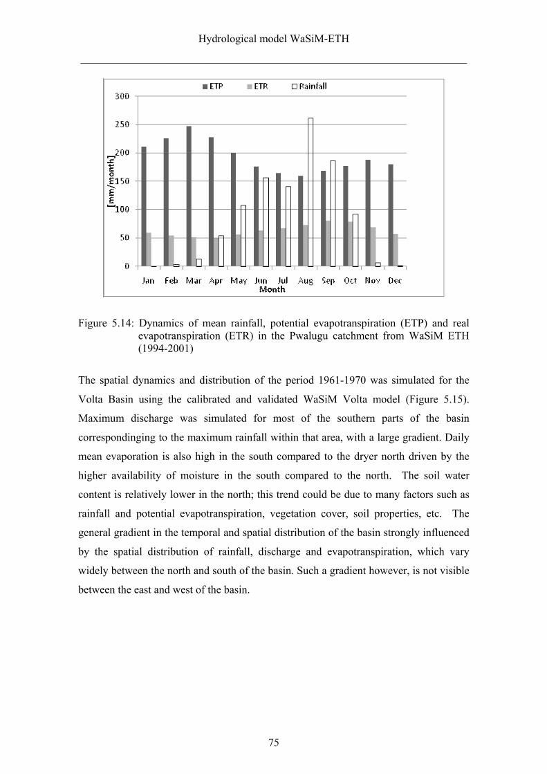
Hydrological model WaSiM-ETH
______________________________________________________________________
75
Figure 5.14: Dynamics of mean rainfall, potential evapotranspiration (ETP) and real
evapotranspiration (ETR) in the Pwalugu catchment from WaSiM ETH (1994-2001)
The spatial dynamics and distribution of the period 1961-1970 was simulated for the
Volta Basin using the calibrated and validated WaSiM Volta model (Figure 5.15).
Maximum discharge was simulated for most of the southern parts of the basin
correspondinging to the maximum rainfall within that area, with a large gradient. Daily
mean evaporation is also high in the south compared to the dryer north driven by the
higher availability of moisture in the south compared to the north. The soil water
content is relatively lower in the north; this trend could be due to many factors such as
rainfall and potential evapotranspiration, vegetation cover, soil properties, etc. The
general gradient in the temporal and spatial distribution of the basin strongly influenced
by the spatial distribution of rainfall, discharge and evapotranspiration, which vary
widely between the north and south of the basin. Such a gradient however, is not visible
between the east and west of the basin.
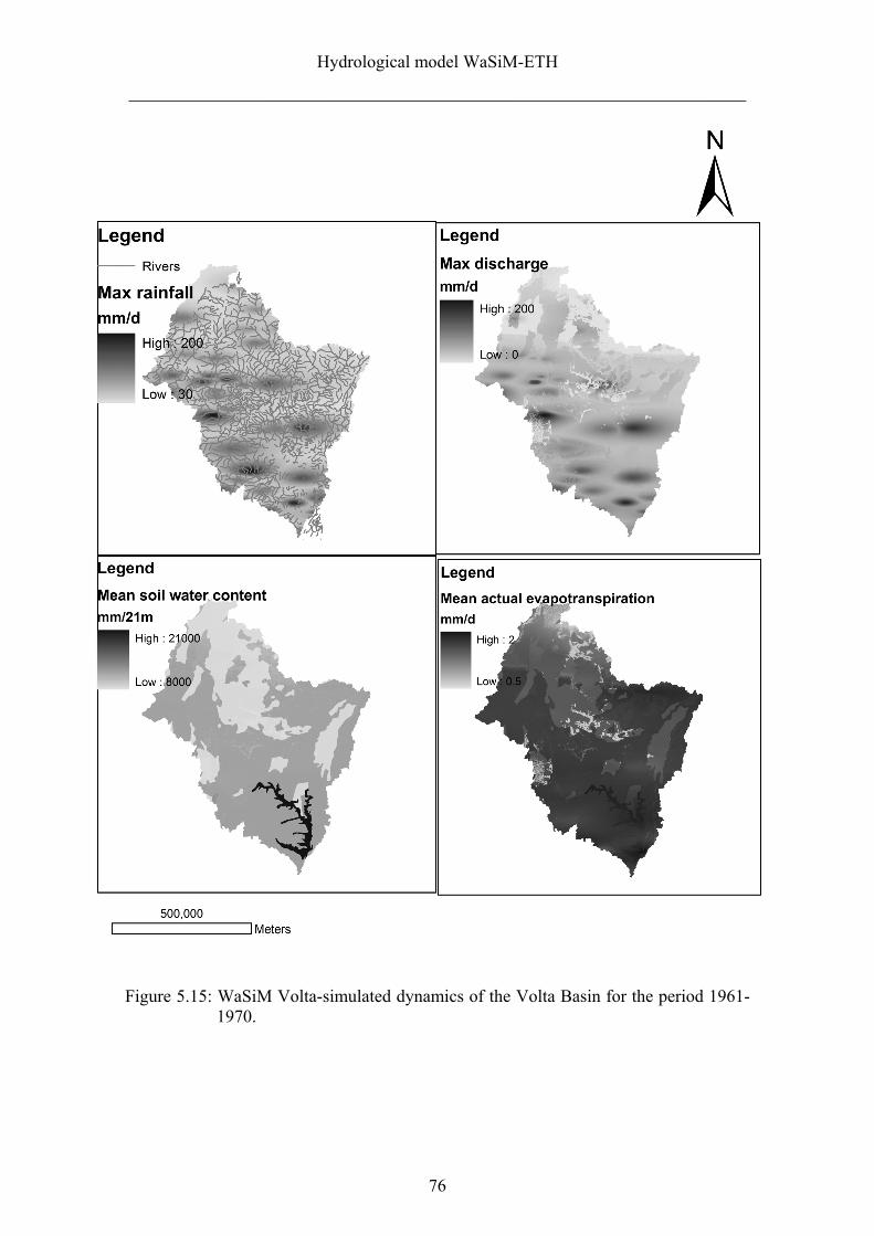
Hydrological model WaSiM-ETH
______________________________________________________________________
76
Figure 5.15: WaSiM Volta-simulated dynamics of the Volta Basin for the period 1961-1970.
Drought in the Volta Basin
______________________________________________________________________
77
6 DROUGHT IN THE VOLTA BASIN
6.1 Introduction
In most parts of West Africa, farmers practice shifting cultivation and traditional bush
fallow systems under a unimodal or bimodal rainfed agriculture. High variability of
rainfall patterns and distribution is the main factor causing fluctuations in food
production in the Volta Basin especially the northern parts. The annual rainfall, which
falls within one rainy season, is erratic both in onset and distribution; the rainy seasons
are characterized by dry spells of varying duration (Kasei, 1995).
Various recent reports on the climate of the sub-region have suggested that
there has been a recovery of the rainy season (Nicholson, 2005). The Intergovernmental
Panel on Climate Change (IPCC) predicts that hot extremes, heat waves, and heavy
precipitation are becoming more frequent in some regions in the world, and that
subtropical regions are likely to receive less rainfall due to climate change (IPCC,
2007). Meteorological and hydrological data from the Volta Basin show a decline in
rainfall amounts and duration of the length of the rainy season. The frequency of rainfall
deficiency has increased since the early 1970s, and moderate to severe drought years
have occurred at approximately 9-year intervals with a reoccurrence of severe droughts.
Notable years of drought extending to 50 % of the basin area or more are 1961, 1970,
1983, 1992 and 2001.
In the early 1970s and mid 1980s, countries in the West African Sahel suffered
from a series of drought years, which had devastating consequences for the inhabitants
of the entire Volta Basin. Average rainfall for the 1982–1985 period was only 381 mm,
less than nearly 60 % of the long-term average (Dugue, 1989).
The years of recurrent drought, high variability in the monsoon rains and
variations in the start and end of the rains as well as their intensities greatly affected
crop production, provoking structural food shortages and hunger. In the early 1980s, 14
out of 18 households studied by Broekhuyse (1983) in the village of Oualaga
(Sanmatenga province, Burkina Faso) had a food deficit of more than 50 %. In Ghana,
food production was below normal in the drought year of 1983 (PPMED 1987). In
Senegal, rice yields decreased rapidly when rainfall was less than average over a 10-
Drought in the Volta Basin
______________________________________________________________________
78
year period (Elston, 1983). In the north of Ghana, inter-annual variation of rainfall is
between 5 % and 45 % in areas across the zone (Kasei 1988).
6.2 Regional climate trends and global climate change
The mean climate of 1951-1980 showed a warmer period compared to the decades
before this period, thus confirming the assumption that global surfaces temperatures
have risen throughout the last century. The highest temperatures of this century have
occurred within the last 10 years affecting the middle and higher latitudes. In poorly
observed regions of Africa, the limited data also show warming temperatures
throughout the 20th century. The Sahelian zone has recorded several decades of below
normal rainfall, especially from the late 1960s to the 1990s, which consequently had a
significant impact on economic development.
According to Henkins et al. (2002), scientists agree on anomalies in the
decadal rainfall but differ on the causes. Some scientists are of the opinion that local
processes (e.g., massive deforestation, desertification, etc.,) are to blame for the drying
pattern observed within West Africa, while others hold external factors (e.g., Sea
Surface Temperatures (SSTs) and global anthropogenic change) responsible.
The Atlantic Multidecadal Oscillation (AMO) has recently been linked to the
anomalies in the western and southern parts of Africa. However, a number of regional
models suggest that there is a stronger link between the warming of the Indian Ocean
SSTs to the drying of the Sahelian zone. A link is thereby suggested between the El
Nino Southern Oscillation (ENSO) and climate change, which is thought to influence
the intensity, duration and return periods of the AMO and the West African climate
(Henkins et al. 2005). In general, ENSO is a disruption of the ocean-atmosphere system
in the tropical Pacific and has an important impact on global weather, and is also known
to cause SST anomalies in the tropical Pacific.
The IPCC reports that different climate models yield different trends and
patterns of the West African climate (IPCC, 2001). Determining the character of the
West African rainfall against a background of large natural variability supported by the
use of imperfect climate models has become the major problem. However, most models
agree that the African continent will experience a temperature increase of 1-3C
throughout the 21st century with some parts recording higher increases. In the face of
Drought in the Volta Basin
______________________________________________________________________
79
increasing temperatures, a further reduction in soil moisture as a result of increased
evapotranspiration is expected (IPCC, 2001).
6.3 Drought in the Volta basin
The Volta Basin is regarded as one of the poorest regions in Africa, with over 80 % of
the total surface area located in Burkina Faso and Ghana. Rainfed and irrigated
agriculture are the principal basis of development for most of the people living in the
basin. The growing population (3 % per annum) is increasing the pressure on land and
water resources. Within the last decade, Burkina Faso (upstream) has improved its
agricultural sector by developing more irrigation farms that depend largely on the
availability of surface water resources. Ghana (downstream) on the other hand is
suffering from the impact of the enhanced use of the water resources upstream by
Burkina Faso, particularly at the Akosombo dam on which Ghana draws for over 80 %
of its energy supply. Low flows resulting in low water levels behind the dam from 1998
and especially in the last 5years have led to a major energy crisis in Ghana in the last
decades, often blamed on the recent development in Burkina Faso. Some also argue that
the recent low flows recorded downstream may have been caused by unreliable rainfall
variations and the poor understanding of these variations (Green Cross International,
2001).
The unreliable rainfall situation creates difficulties in meeting food production
targets, and requires that more attention is paid to agricultural programmes to ensure
food security. Nearly 90 % of the area is under rainfed farming. The onset of the
monsoon determines the planting time, and the subsequent temporal distribution of
rainfall greatly influences the growth and development of the crop. The sowing time in
the north starts in May, and by June the monsoon activity covers the entire country.
The length of the growing season in the north depends on the withdrawal of the
monsoon rainfall activity sometime in October. Initial studies on drought using the
probabilities of dry spell runs showed that the north of the basin as a whole is prone to
drought conditions (Kasei et al. 1995). In the middle part of the basin (Tamale), a dry
spell of 7 days can be expected to occur once a year in June and once in every four
years in September at the peak of the rains (Kasei, 1993). Several trend analyses of
precipitation were performed for West Africa. According to Le Barbé and Lebel (1997),
Drought in the Volta Basin
______________________________________________________________________
80
Servant et al. (1998), or Amani (2001) and Oguntunde et al. (2007), an overall tendency
towards a decrease in rainfall has been observed since the discontinuity of the 1960s and
70s. The decrease in rainfall lies between 15 and 30 % (Nicholson, 1993) and the 1980s
were the driest period of the 20th century in West Africa (Hulme et al. 2001). Thus,
developing a method for predicting the probability of less than the minimum amount in
rainfall would be useful. Such methods could be used as a basis for comparison of
drought hazards during the rainy seasons in different areas. It is well known that
consecutive spells of low rainfall, which result in drought conditions, often occur in the
same areas. Simpler criteria close to those of Sastry (1976), which use the frequency
and probability of the occurrence of a specified number of consecutive dry days based
on the evapotranspiration parameter, could be developed for such analyses.
The need to analyze rainfall with regard to probable wet and dry periods in
particularly important in areas characterized by high spatial and temporal variability.
Oladipo, (1985) showed that when one is interested in meteorological applications,
simple indices with rainfall as the only input perform as well as the more complicated
drought indices such as those of Palmer (1965) and Bhalme and Mooley (1980).
Drought is a recurrent phenomenon that will continue to affect different parts
of the Volta Basin at unexpected intervals. By virtue of its characteristics,
manifestation and impacts on the society, drought is a complex natural hazard. Drought
detection and monitoring is not an easy exercise for a number of reasons. What
constitutes drought? Drought means different things to different people. Regardless of
the divergence of views concerning drought definition, the simplest starting point to
quantify and qualify drought is to regard it as a relative meteorological phenomenon
that is generally nothing but a rainfall deficiency that tends to affect adversely water
supplies, crop and livestock production, causing food shortages and disruption of
economic activities. Hence, the aim of this part of the study is to characterize
meteorological droughts in the Volta Basin to provide a guide for sustainable water
resources management.
6.4 Rainfall anomalies in the Volta Basin
Climatic extremes that characterize this region are recurring drought, harmattan (a hot,
dry, usually dusty wind that blows from the northeast or east in the southern Sahara,
Drought in the Volta Basin
______________________________________________________________________
81
mainly in winter), and sometimes torrential flooding. Highest precipitation levels occur
in the south and can reach an annual 2,000 mm, while levels in the driest regions in the
north can be as low as 200 mm annually (see section 2).
Around 80 % of annual rainfall occurs from July to September with most
places experiencing monsoonal rains. Mean annual precipitation ranges from less than
300 mm up to more than 1500 mm, showing a strong north-south gradient, with higher
rainfall amounts in the tropical south and smaller amounts in the semi-arid north of the
basin. In addition, in the south-western corner of Ghana, which is actually not part of
the Volta Basin, annual precipitation exceeds 2100 mm, whereas in south-eastern Ghana
it is less than 800 mm (Jung 2006). This is a clear indication that not only a north-south
gradient (Figure 6.2) exists, but also a quite strong west-east gradient (Figure 6.3) with
regard to the transect (Figure 6.1) chosen.
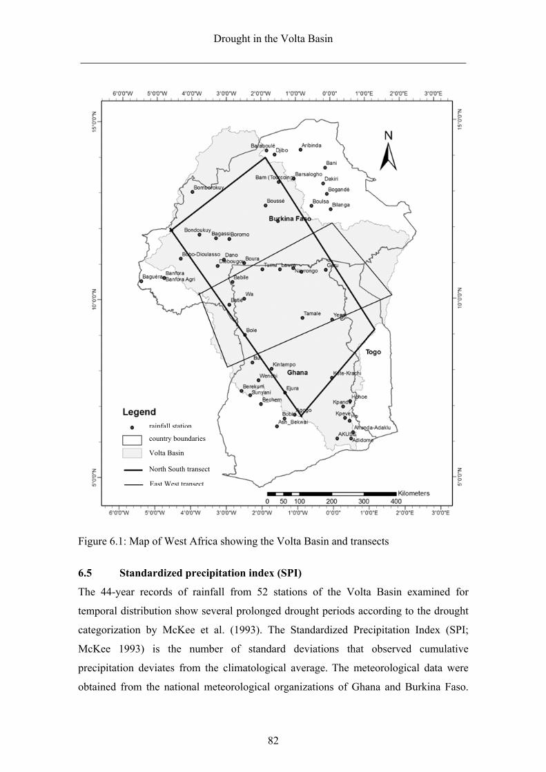
Drought in the Volta Basin
______________________________________________________________________
82
Figure 6.1: Map of West Africa showing the Volta Basin and transects
6.5 Standardized precipitation index (SPI)
The 44-year records of rainfall from 52 stations of the Volta Basin examined for
temporal distribution show several prolonged drought periods according to the drought
categorization by McKee et al. (1993). The Standardized Precipitation Index (SPI;
McKee 1993) is the number of standard deviations that observed cumulative
precipitation deviates from the climatological average. The meteorological data were
obtained from the national meteorological organizations of Ghana and Burkina Faso.
rainfall station
country boundaries
Volta Basin
East West transect
North South transect
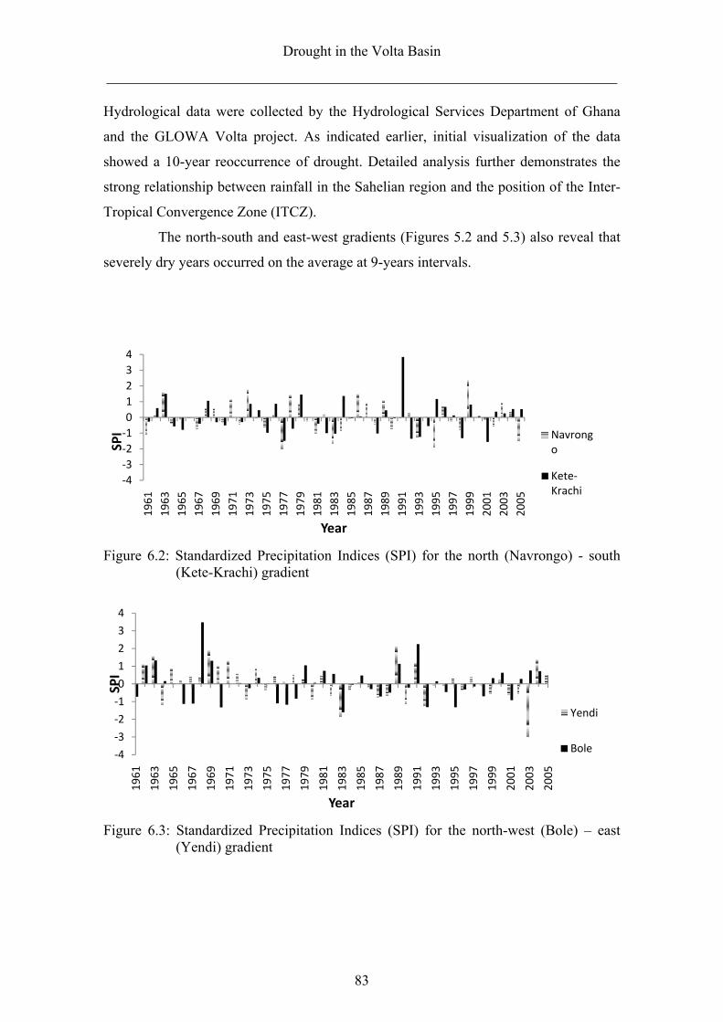
Drought in the Volta Basin
______________________________________________________________________
83
Hydrological data were collected by the Hydrological Services Department of Ghana
and the GLOWA Volta project. As indicated earlier, initial visualization of the data
showed a 10-year reoccurrence of drought. Detailed analysis further demonstrates the
strong relationship between rainfall in the Sahelian region and the position of the Inter-
Tropical Convergence Zone (ITCZ).
The north-south and east-west gradients (Figures 5.2 and 5.3) also reveal that
severely dry years occurred on the average at 9-years intervals.
Figure 6.2: Standardized Precipitation Indices (SPI) for the north (Navrongo) - south (Kete-Krachi) gradient
Figure 6.3: Standardized Precipitation Indices (SPI) for the north-west (Bole) – east (Yendi) gradient
‐4
‐3
‐2
‐1
0
1
2
3
4
1961
1963
1965
1967
1969
1971
1973
1975
1977
1979
1981
1983
1985
1987
1989
1991
1993
1995
1997
1999
2001
2003
2005
SPI
Year
Navrongo
Kete‐Krachi
‐4
‐3
‐2
‐1
0
1
2
3
4
1961
1963
1965
1967
1969
1971
1973
1975
1977
1979
1981
1983
1985
1987
1989
1991
1993
1995
1997
1999
2001
2003
2005
SPI
Year
Yendi
Bole
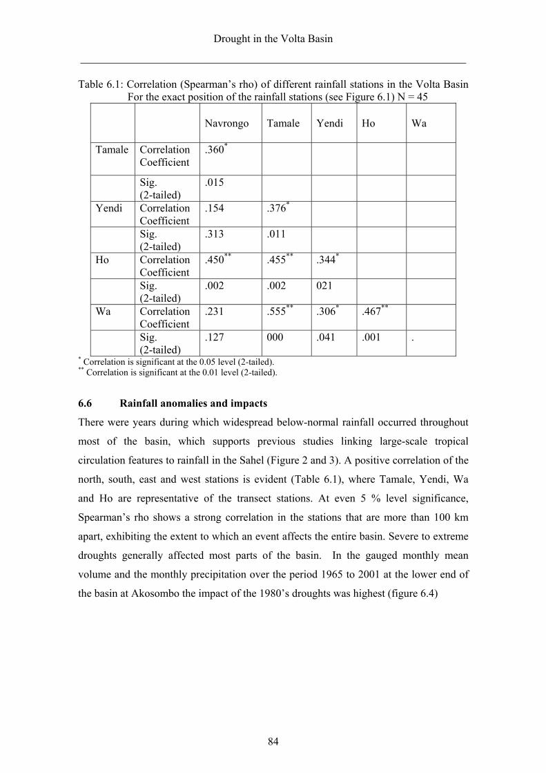
Drought in the Volta Basin
______________________________________________________________________
84
Table 6.1: Correlation (Spearman’s rho) of different rainfall stations in the Volta Basin For the exact position of the rainfall stations (see Figure 6.1) N = 45
Navrongo Tamale Yendi Ho Wa
Tamale Correlation Coefficient
.360*
Sig. (2-tailed)
.015
Yendi Correlation Coefficient
.154 .376*
Sig. (2-tailed)
.313 .011
Ho Correlation Coefficient
.450** .455** .344*
Sig. (2-tailed)
.002 .002 021
Wa Correlation Coefficient
.231 .555** .306* .467**
Sig. (2-tailed)
.127 000 .041 .001 .
* Correlation is significant at the 0.05 level (2-tailed). ** Correlation is significant at the 0.01 level (2-tailed).
6.6 Rainfall anomalies and impacts
There were years during which widespread below-normal rainfall occurred throughout
most of the basin, which supports previous studies linking large-scale tropical
circulation features to rainfall in the Sahel (Figure 2 and 3). A positive correlation of the
north, south, east and west stations is evident (Table 6.1), where Tamale, Yendi, Wa
and Ho are representative of the transect stations. At even 5 % level significance,
Spearman’s rho shows a strong correlation in the stations that are more than 100 km
apart, exhibiting the extent to which an event affects the entire basin. Severe to extreme
droughts generally affected most parts of the basin. In the gauged monthly mean
volume and the monthly precipitation over the period 1965 to 2001 at the lower end of
the basin at Akosombo the impact of the 1980’s droughts was highest (figure 6.4)
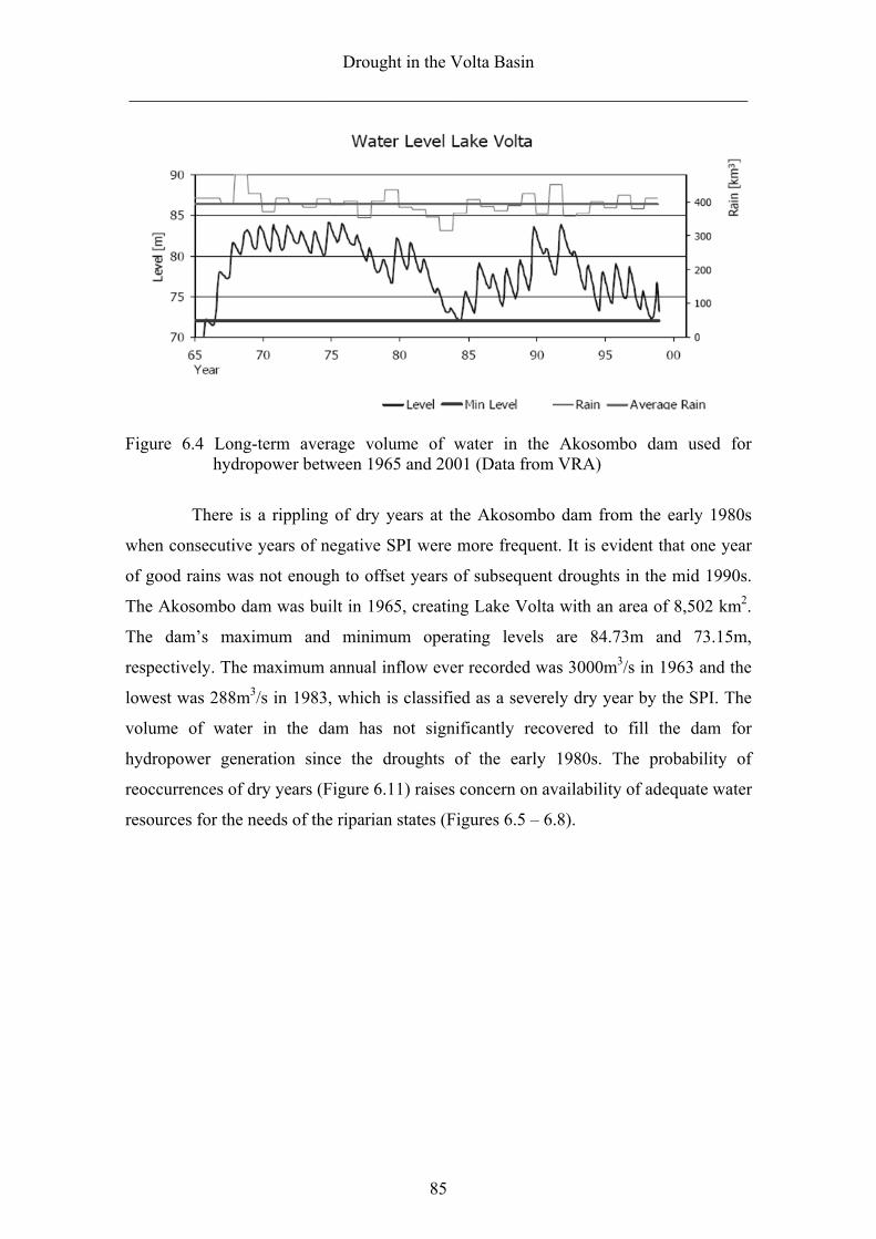
Drought in the Volta Basin
______________________________________________________________________
85
Figure 6.4 Long-term average volume of water in the Akosombo dam used for hydropower between 1965 and 2001 (Data from VRA)
There is a rippling of dry years at the Akosombo dam from the early 1980s
when consecutive years of negative SPI were more frequent. It is evident that one year
of good rains was not enough to offset years of subsequent droughts in the mid 1990s.
The Akosombo dam was built in 1965, creating Lake Volta with an area of 8,502 km2.
The dam’s maximum and minimum operating levels are 84.73m and 73.15m,
respectively. The maximum annual inflow ever recorded was 3000m3/s in 1963 and the
lowest was 288m3/s in 1983, which is classified as a severely dry year by the SPI. The
volume of water in the dam has not significantly recovered to fill the dam for
hydropower generation since the droughts of the early 1980s. The probability of
reoccurrences of dry years (Figure 6.11) raises concern on availability of adequate water
resources for the needs of the riparian states (Figures 6.5 – 6.8).
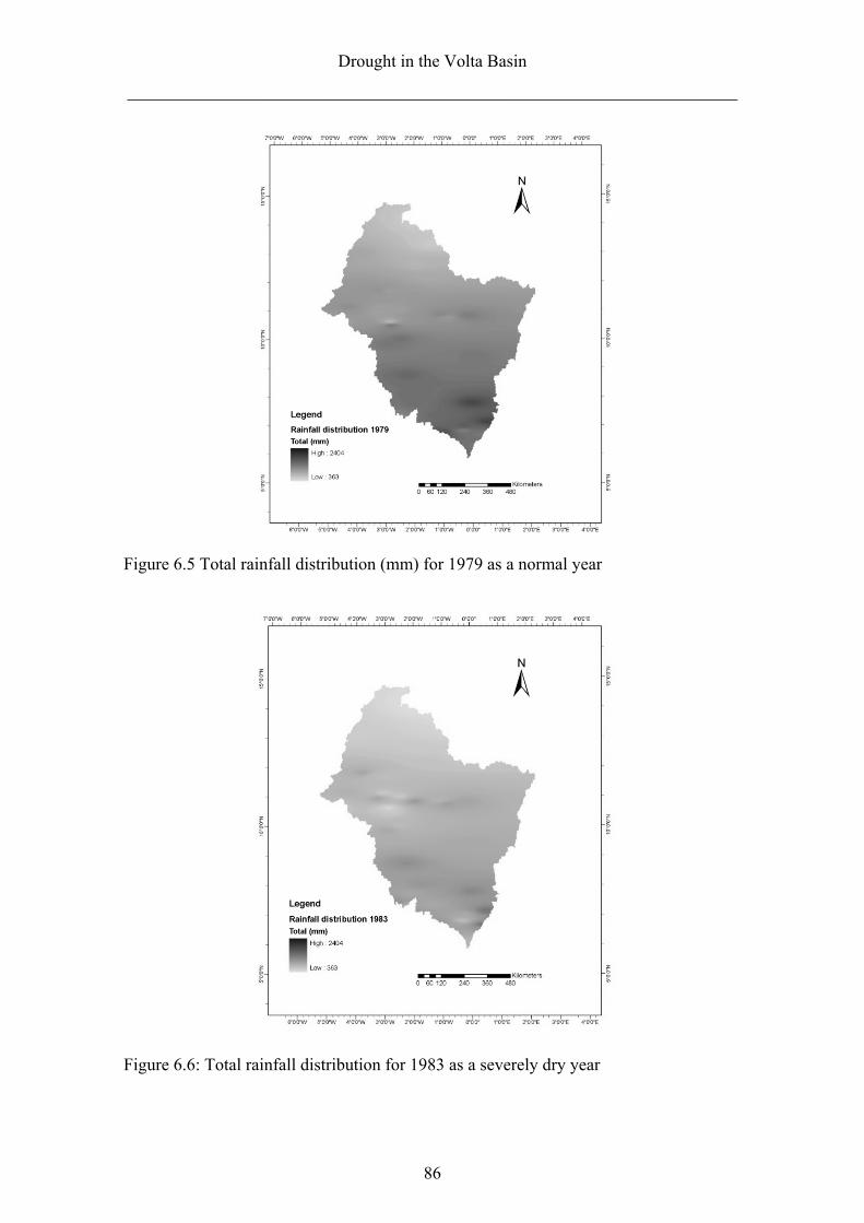
Drought in the Volta Basin
______________________________________________________________________
86
Figure 6.5 Total rainfall distribution (mm) for 1979 as a normal year
Figure 6.6: Total rainfall distribution for 1983 as a severely dry year
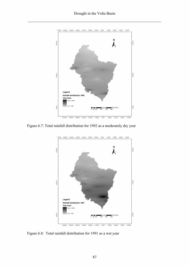
Drought in the Volta Basin
______________________________________________________________________
87
Figure 6.7: Total rainfall distribution for 1992 as a moderately dry year
Figure 6.8: Total rainfall distribution for 1991 as a wet year
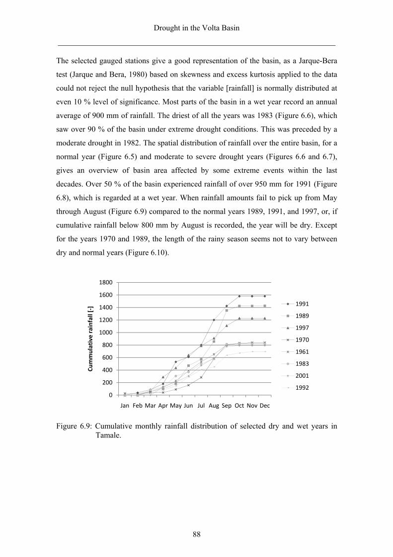
Drought in the Volta Basin
______________________________________________________________________
88
The selected gauged stations give a good representation of the basin, as a Jarque-Bera
test (Jarque and Bera, 1980) based on skewness and excess kurtosis applied to the data
could not reject the null hypothesis that the variable [rainfall] is normally distributed at
even 10 % level of significance. Most parts of the basin in a wet year record an annual
average of 900 mm of rainfall. The driest of all the years was 1983 (Figure 6.6), which
saw over 90 % of the basin under extreme drought conditions. This was preceded by a
moderate drought in 1982. The spatial distribution of rainfall over the entire basin, for a
normal year (Figure 6.5) and moderate to severe drought years (Figures 6.6 and 6.7),
gives an overview of basin area affected by some extreme events within the last
decades. Over 50 % of the basin experienced rainfall of over 950 mm for 1991 (Figure
6.8), which is regarded at a wet year. When rainfall amounts fail to pick up from May
through August (Figure 6.9) compared to the normal years 1989, 1991, and 1997, or, if
cumulative rainfall below 800 mm by August is recorded, the year will be dry. Except
for the years 1970 and 1989, the length of the rainy season seems not to vary between
dry and normal years (Figure 6.10).
Figure 6.9: Cumulative monthly rainfall distribution of selected dry and wet years in Tamale.
0
200
400
600
800
1000
1200
1400
1600
1800
Jan Feb Mar Apr May Jun Jul Aug Sep Oct Nov Dec
Cummulative rainfall [‐] 1991
1989
1997
1970
1961
1983
2001
1992
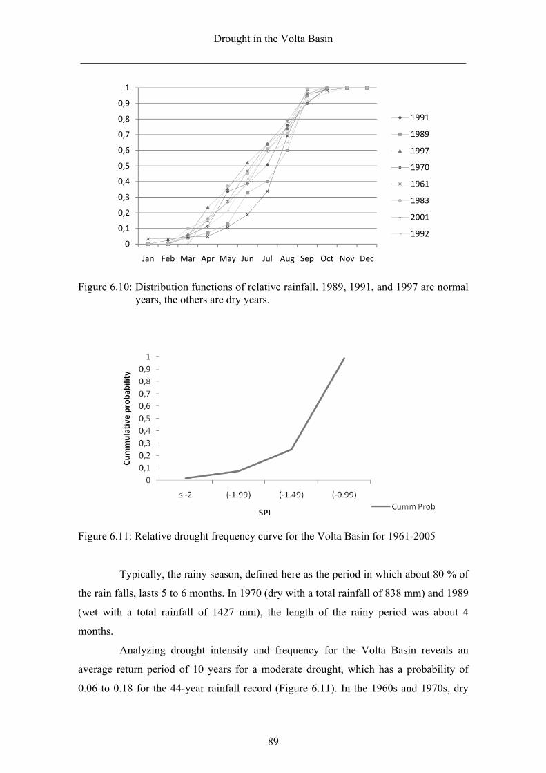
Drought in the Volta Basin
______________________________________________________________________
89
Figure 6.10: Distribution functions of relative rainfall. 1989, 1991, and 1997 are normal years, the others are dry years.
Figure 6.11: Relative drought frequency curve for the Volta Basin for 1961-2005
Typically, the rainy season, defined here as the period in which about 80 % of
the rain falls, lasts 5 to 6 months. In 1970 (dry with a total rainfall of 838 mm) and 1989
(wet with a total rainfall of 1427 mm), the length of the rainy period was about 4
months.
Analyzing drought intensity and frequency for the Volta Basin reveals an
average return period of 10 years for a moderate drought, which has a probability of
0.06 to 0.18 for the 44-year rainfall record (Figure 6.11). In the 1960s and 1970s, dry
0
0,1
0,2
0,3
0,4
0,5
0,6
0,7
0,8
0,9
1
Jan Feb Mar Apr May Jun Jul Aug Sep Oct Nov Dec
1991
1989
1997
1970
1961
1983
2001
1992
Drought in the Volta Basin
______________________________________________________________________
90
years occurred at an interval of 3-4 years, but from the early 1980s till 2006, dry years
occurred almost every other year, indicating an increase in the frequency of dry years in
the basin with a probability of 0.7. The drought of 1983/84, which affected the whole
region, had a much lower probability compared to other drought events. The drought
intensity (Figure 6.2 and 6.3) with SPI lower than -2.0 usually affected nearly 75 % of
the region. This would most often show that major parts of the region experience
extreme drought conditions during these years. The droughts of 1961 and 1970 had a
much higher probability of occurrence (0.7). The areal extent of extreme drought
conditions was about 90 % during this drought period. The drought of 2001 seems to
have had a relatively high probability of 0.17 compared to that of 1992, which had a
probability of 0.06.
Dry years have become more frequent since the beginning of the 1980s and
have occurred at shorter intervals. The areal extents of this dryness, though not severe,
have been increasing over last 20 years. Between 1983 and 2001, the basin experienced
at least 4 moderately dry years covering over 50 % of the area.
Changes in hydrology and risks for water resources in the Volta Basin
_____________________________________________________________________
91
7 CHANGES IN HYDROLOGY AND RISKS FOR WATER
RESOURCES IN THE VOLTA BASIN
7.1 Introduction
The International Union for Conservation of Nature (IUCN) used in their report
“Reducing West Africa’s Vulnerability to Climate Impacts on Water Resources,
Wetlands and Desertification” in 2004 three main reasons why the changes in climate
and hydrology need to be well understood and managed: (1) the significant
contribution of rainfed agriculture to the region’s economy, (2) the poor level of water
control, and (3) the poor replenishment of reservoirs on which some countries depend
heavily for the generation of hydropower and the electricity supply to industry and
households. In general, the national economies of many West African states are
directly affected by the variations in climate.
The climate of West Africa, particularly in the Sahelian zone of which much
of the Volta is part, has been undergoing recurrent variations of significant magnitude,
particularly since the early 1970’s. According to the IUCN (2004), the region has
experienced a marked decline in rainfall over the period 1961- 2000 and hydrometric
series around 1968-1972, with 1970 as a transitional year. The IUCN also found a
decline in average rainfall before and after 1970 ranging from 15 % to over 30 %
depending on the area. This situation resulted in a 200-km southward shift in isohyets.
Average discharge in the region’s major rivers underwent concomitant and highly
pronounced to average decline in the range of 40-60 % in discharge since the early
1970s.
Statistically, significant changes have been realized in the last century
(Oguntunde et al., 2006). As the hydrological conditions in the Volta Basin have not
been very favorable in the last decade, it has become necessary to pay attention to
water management strategies, as problems may arise if this situation continues or shifts
into more water-stressful conditions as predicted by some climate model ensembles
used by IPCC (2007) for the region. If the general agreement that hydrological
conditions across the world are changing, then concepts on water management need to
fit the changing situations. The growing number of reservoirs in the Volta Basin would
need to be improved, and flexible methods of operations are required.
Changes in hydrology and risks for water resources in the Volta Basin
_____________________________________________________________________
92
Major sources of water in the Volta River system and riparian countries consist of
natural and induced rainfall (from cloud seeding), rivers, streams, lakes, groundwater
and artificial impounded water (dams, dug-outs and reservoirs). The estimation of
direct discharge to the system is based on the assumption that discharge occurs
when rainfall amounts and intensities surpass infiltration rates and subsurface
saturation, balanced by actual evapotranspiration. Analyses of rainfall data from
various stations within the Volta River system indicate that the months in which
precipitation exceeds evapotranspiration are usually June, July, August, and
September. The annual recharge for the river system ranges from 13 % to 16 % of
the mean annual precipitation.
Throughout the Volta Basin, over the past decades, dams and reservoirs have
been constructed to mobilize water for agricultural and hydroelectricity purposes. The
number of large and small dams continues to increase as the population grows.
Increasing use of water and uncertainty in precipitation in the basin threatens present
sustainable programs focused on water management. Several large dams have been
constructed (e.g. Akosombo and Bagri) and some are still being constructed (e.g., Bui)
in the Volta River system with the primary purpose of generating electricity. The
damming of the Volta River at Akosombo lake covering an area of approximately
8,500 km2 is regarded as one of the largest man-made lakes in the world today .
A smaller and shallower impoundment next to the Akosombo is the Kpong Head pond,
covering an area of roughly 38 km2 at Kpong, 20 km downstream of Akosombo. Bui,
which is north-west of Akosombo, is under construction and due by 2011. The riparian
states of the Volta (e.g., Benin) depend on hydropower from dams built on other
tributaries of the Volta, while many more like the Pouya (Natitingou) on the Yéripao
are planned. The Fresh water needs of the inhabitants of the basin come from within
the basin, and hence a supply shortfall like that in 2002 and 2003 could mean
catastrophic consequences for the city water supply, e.g., in Burkina Faso, and severe
energy crises in Ghana.
In recent times, there has been immense pressure on Burkina Faso to
increase the number of dams in the Volta Basin to meet the country’s demand for
fresh water. As a result, there are now an estimated 600 dams and 1,400 dugouts
with a total storage potential of 4.7 km3, and about 10,484 wells of which 8,020
Changes in hydrology and risks for water resources in the Volta Basin
_____________________________________________________________________
93
are in good condition. The volume stored annually in these reservoirs is about 2.490
km3, which is about 25 % of total discharge. With respect to hydropower generation,
13 locations have been identified in the country, and 10 are located within the Volta
Basin. A total of 125.9 GWh/yr is expected to be generated from these hydro-power
stations. A recent survey by Direction de l'inventaire des ressources hydrauliques
(DIRH) indicates that several planned irrigation projects covering a total area of 1,045
ha will require about 65.3 million m3 water (IUCN, 2004).
7.2 Climate change
Climate change may have a large impact on water resources, and that could ultimately
affect fundamental drivers of the hydrological cycle. The use of hydrological models
that depend largely on the outputs of the climate, offer platforms on which climate
impacts could be studied. The climate models popularly used to derive or make
projections into the future are the General Circulation Model (GCM). The GCM is
basically a mathematical model based on the general circulation of the planetary
atmosphere and ocean, which integrate the rotations of the sphere. According to
Thorpe (2005), GCMs are among the best tools used for forecasting the weather,
understanding the climate and projecting changes in climate.
Derived from the atmospheric global circulation models (AGCMs) and the
atmosphere-ocean coupled GCMs (AOGCMs) are the HADCM, GFDL, CM2.X,
ECHAM, among others, used for the study and simulation of the present climate and
for the projections of the future climate. In the simulation of the hydrology of a
watershed, credible input parameters of climate are essential for good results. Outputs
of GCMs, however, have a spatial resolution of 250 km, offering only very coarse data
for the study of small watersheds. According to Sintondji (2005) and Busche et al.
(2005), GCMs have flaws for events of heavy rainfall in respect to their exceeding
thresholds and frequencies. It is also evident that local or regional climates are
influenced not only by the atmospheric processes, but are also greatly influenced by
land-sea interaction, land use and the topography, which are poorly presented in
GCMs due to their coarse spatial resolutions (Storch et al. 1993)
Regional Climate Models (RCMs) have been derived from the coarse GCMs
to much higher resolutions. The process of downscaling of GCMs to meso-scales or
Changes in hydrology and risks for water resources in the Volta Basin
_____________________________________________________________________
94
regional scales enables the downscaled regional climate model to adequately simulate
the physical processes consistently with GCMs on a large scale (Mearns et al. 2004).
Since parameters of land use and topography are crucial in the efficiency of the RCMs,
the higher the resolution of the RCMs, the better the simulation of the climate and
ultimately, a better hydrological simulation is achieved. Some of the RCMs that have
been popular in West Africa are REMO, MM5 and PRECIS.
7.3 Regional climate scenarios – MM5
The regional climate model MM5 is a meso-scale model derived from the GCM-
ECHAM4 recently developed for the assessments of the impacts of environmental and
climate change on water resources on the Volta Basin of West Africa. The MM5 is a
brain child of the cooperation of the Pennsylvania State University (PSU) and the
National Center for Atmospheric Research (NCAR) of the USA. According to Grell et
al. (1995), the MM5 non-hydrostatic or hydrostatic (available only in version 2) is
designed with the initial and lateral boundary conditions of a region to simulate or
predict meso-scale and regional-scale atmospheric circulation.
The GLOWA-Volta project (GVP) executed by the Center for Development
Research (ZEF), Germany, ran MM5 with the initial and lateral boundary conditions
derived from the ECHAM4 runs of the time slice 1860-2100, and based on IPCC’s
IS92a (assuming an annual increase in CO2 of 1 %, and doubling of CO2 in 90 years
(May and Rockner, 2001; cited in Jung, 2006). Using future climate scenario and
girded monthly observational dataset from the East Anglia Climate Research Unit
(CRU), UK, the model was calibrated to 0.5o x 0.5o resolution. GVP further down-
scaled the MM5 model for the Volta Basin to finer resolutions of 9 km x9 km, and for
some watersheds within the basin to 3 km x 3 km. Details of the setup, coupling and
simulation are available in Kunstmann and Jung (2005) and Jung (2006).
A good agreement was reported between the ECHAM4-MM5 simulated
climate and the CRU data sets for 1961-1990. According to Jung (2006), simulated
temperature was slightly higher in the Sahara during the wet seasons and for the humid
south during the dry season, while rainfall was generally comparable except for higher
rainfall events that were underestimated. Between ECHAM4 and MM5, 1990-2000
simulations revealed that temperature was generally over estimated and rainfall under
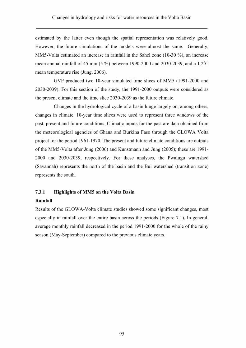
Changes in hydrology and risks for water resources in the Volta Basin
_____________________________________________________________________
95
estimated by the latter even though the spatial representation was relatively good.
However, the future simulations of the models were almost the same. Generally,
MM5-Volta estimated an increase in rainfall in the Sahel zone (10-30 %), an increase
mean annual rainfall of 45 mm (5 %) between 1990-2000 and 2030-2039, and a 1.2oC
mean temperature rise (Jung, 2006).
GVP produced two 10-year simulated time slices of MM5 (1991-2000 and
2030-2039). For this section of the study, the 1991-2000 outputs were considered as
the present climate and the time slice 2030-2039 as the future climate.
Changes in the hydrological cycle of a basin hinge largely on, among others,
changes in climate. 10-year time slices were used to represent three windows of the
past, present and future conditions. Climatic inputs for the past are data obtained from
the meteorological agencies of Ghana and Burkina Faso through the GLOWA Volta
project for the period 1961-1970. The present and future climate conditions are outputs
of the MM5-Volta after Jung (2006) and Kunstmann and Jung (2005); these are 1991-
2000 and 2030-2039, respectively. For these analyses, the Pwalugu watershed
(Savannah) represents the north of the basin and the Bui watershed (transition zone)
represents the south.
7.3.1 Highlights of MM5 on the Volta Basin
Rainfall
Results of the GLOWA-Volta climate studies showed some significant changes, most
especially in rainfall over the entire basin across the periods (Figure 7.1). In general,
average monthly rainfall decreased in the period 1991-2000 for the whole of the rainy
season (May-September) compared to the previous climate years.
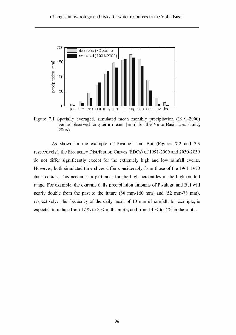
Changes in hydrology and risks for water resources in the Volta Basin
_____________________________________________________________________
96
Figure 7.1 Spatially averaged, simulated mean monthly precipitation (1991-2000) versus observed long-term means [mm] for the Volta Basin area (Jung, 2006)
As shown in the example of Pwalugu and Bui (Figures 7.2 and 7.3
respectively), the Frequency Distribution Curves (FDCs) of 1991-2000 and 2030-2039
do not differ significantly except for the extremely high and low rainfall events.
However, both simulated time slices differ considerably from those of the 1961-1970
data records. This accounts in particular for the high percentiles in the high rainfall
range. For example, the extreme daily precipitation amounts of Pwalugu and Bui will
nearly double from the past to the future (80 mm-160 mm) and (52 mm-78 mm),
respectively. The frequency of the daily mean of 10 mm of rainfall, for example, is
expected to reduce from 17 % to 8 % in the north, and from 14 % to 7 % in the south.
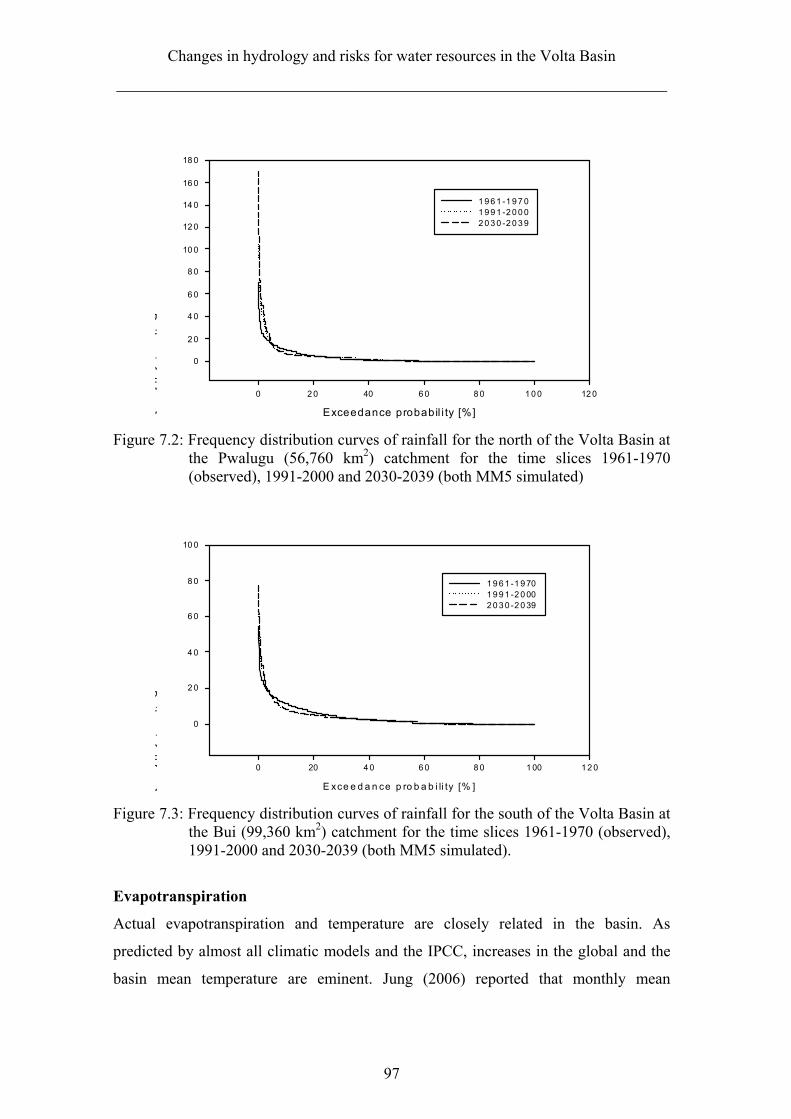
Changes in hydrology and risks for water resources in the Volta Basin
_____________________________________________________________________
97
Exceedance probabil i ty [%]
0 2 0 40 6 0 8 0 1 0 0 12 0
Dil
if
ll[]
0
2 0
4 0
6 0
8 0
10 0
12 0
14 0
16 0
18 0
1 9 6 1 -1 9 7 01 9 9 1 -2 0 0 02 0 3 0 -2 0 3 9
Figure 7.2: Frequency distribution curves of rainfall for the north of the Volta Basin at the Pwalugu (56,760 km2) catchment for the time slices 1961-1970 (observed), 1991-2000 and 2030-2039 (both MM5 simulated)
E xce e d a n ce p ro b a b i li ty [% ]
0 20 4 0 6 0 8 0 1 00 1 2 0
Dil
if
ll[
]
0
2 0
4 0
6 0
8 0
10 0
1 9 6 1 -1 9 701 9 9 1 -2 0 002 0 3 0 -2 0 39
Figure 7.3: Frequency distribution curves of rainfall for the south of the Volta Basin at the Bui (99,360 km2) catchment for the time slices 1961-1970 (observed), 1991-2000 and 2030-2039 (both MM5 simulated).
Evapotranspiration
Actual evapotranspiration and temperature are closely related in the basin. As
predicted by almost all climatic models and the IPCC, increases in the global and the
basin mean temperature are eminent. Jung (2006) reported that monthly mean
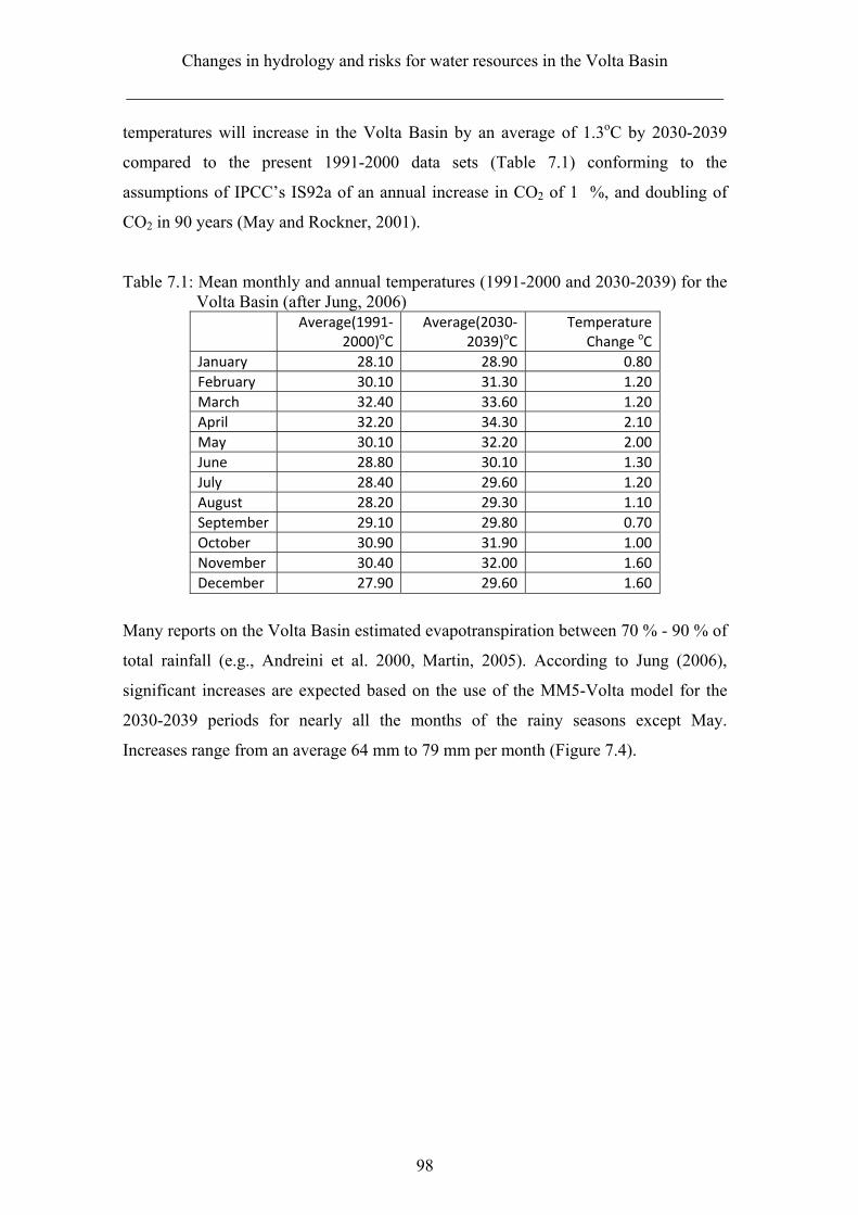
Changes in hydrology and risks for water resources in the Volta Basin
_____________________________________________________________________
98
temperatures will increase in the Volta Basin by an average of 1.3oC by 2030-2039
compared to the present 1991-2000 data sets (Table 7.1) conforming to the
assumptions of IPCC’s IS92a of an annual increase in CO2 of 1 %, and doubling of
CO2 in 90 years (May and Rockner, 2001).
Table 7.1: Mean monthly and annual temperatures (1991-2000 and 2030-2039) for the Volta Basin (after Jung, 2006)
Many reports on the Volta Basin estimated evapotranspiration between 70 % - 90 % of
total rainfall (e.g., Andreini et al. 2000, Martin, 2005). According to Jung (2006),
significant increases are expected based on the use of the MM5-Volta model for the
2030-2039 periods for nearly all the months of the rainy seasons except May.
Increases range from an average 64 mm to 79 mm per month (Figure 7.4).
Average(1991‐2000)oC
Average(2030‐2039)oC
Temperature Change oC
January 28.10 28.90 0.80
February 30.10 31.30 1.20
March 32.40 33.60 1.20
April 32.20 34.30 2.10
May 30.10 32.20 2.00
June 28.80 30.10 1.30
July 28.40 29.60 1.20
August 28.20 29.30 1.10
September 29.10 29.80 0.70
October 30.90 31.90 1.00
November 30.40 32.00 1.60
December 27.90 29.60 1.60
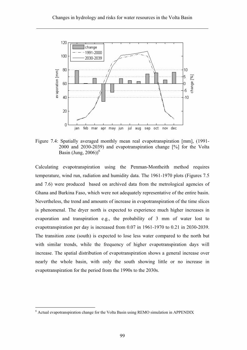
Changes in hydrology and risks for water resources in the Volta Basin
_____________________________________________________________________
99
Figure 7.4: Spatially averaged monthly mean real evapotranspiration [mm], (1991-2000 and 2030-2039) and evapotranspiration change [%] for the Volta Basin (Jung, 2006))6
Calculating evapotranspiration using the Penman-Montheith method requires
temperature, wind run, radiation and humidity data. The 1961-1970 plots (Figures 7.5
and 7.6) were produced based on archived data from the metrological agencies of
Ghana and Burkina Faso, which were not adequately representative of the entire basin.
Nevertheless, the trend and amounts of increase in evapotranspiration of the time slices
is phenomenal. The dryer north is expected to experience much higher increases in
evaporation and transpiration e.g., the probability of 3 mm of water lost to
evapotranspiration per day is increased from 0.07 in 1961-1970 to 0.21 in 2030-2039.
The transition zone (south) is expected to lose less water compared to the north but
with similar trends, while the frequency of higher evapotranspiration days will
increase. The spatial distribution of evapotranspiration shows a general increase over
nearly the whole basin, with only the south showing little or no increase in
evapotranspiration for the period from the 1990s to the 2030s.
6 Actual evapotranspiration change for the Volta Basin using REMO simulation in APPENDIX
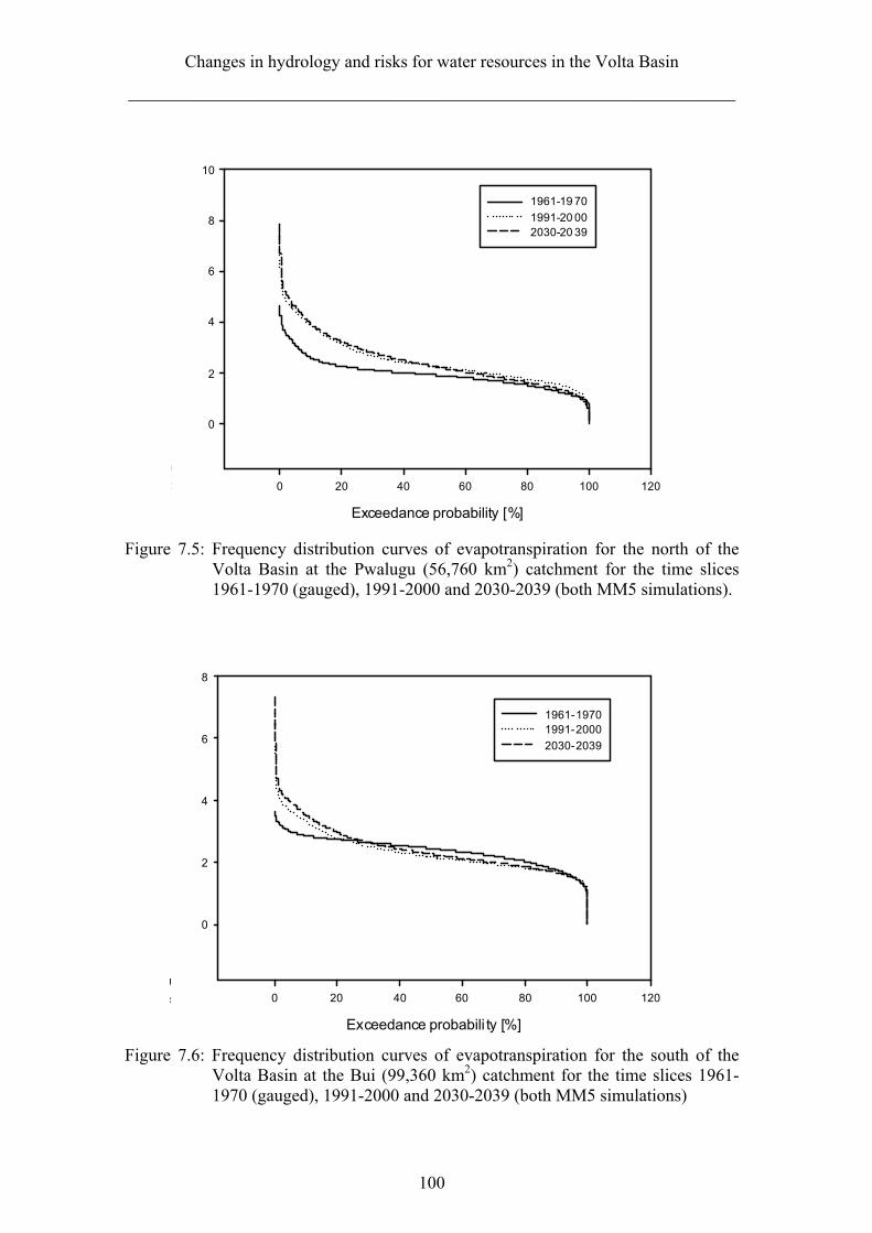
Changes in hydrology and risks for water resources in the Volta Basin
_____________________________________________________________________
100
Figure 7.5: Frequency distribution curves of evapotranspiration for the north of the Volta Basin at the Pwalugu (56,760 km2) catchment for the time slices 1961-1970 (gauged), 1991-2000 and 2030-2039 (both MM5 simulations).
Exceedance probabili ty [%]
0 20 40 60 80 100 120
Dil
0
2
4
6
8
1961-19701991-2000
2030-2039
Figure 7.6: Frequency distribution curves of evapotranspiration for the south of the Volta Basin at the Bui (99,360 km2) catchment for the time slices 1961-1970 (gauged), 1991-2000 and 2030-2039 (both MM5 simulations)
Exceedance probability [%]
0 20 40 60 80 100 120
Dil
0
2
4
6
8
10
1961-19 70
1991-20 002030-20 39
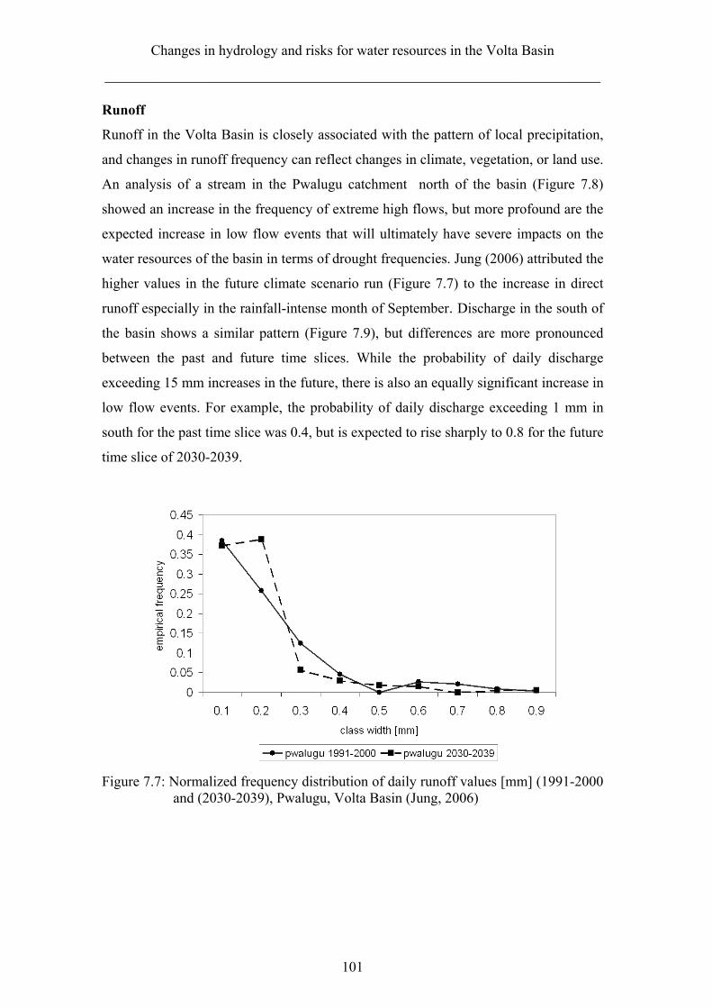
Changes in hydrology and risks for water resources in the Volta Basin
_____________________________________________________________________
101
Runoff
Runoff in the Volta Basin is closely associated with the pattern of local precipitation,
and changes in runoff frequency can reflect changes in climate, vegetation, or land use.
An analysis of a stream in the Pwalugu catchment north of the basin (Figure 7.8)
showed an increase in the frequency of extreme high flows, but more profound are the
expected increase in low flow events that will ultimately have severe impacts on the
water resources of the basin in terms of drought frequencies. Jung (2006) attributed the
higher values in the future climate scenario run (Figure 7.7) to the increase in direct
runoff especially in the rainfall-intense month of September. Discharge in the south of
the basin shows a similar pattern (Figure 7.9), but differences are more pronounced
between the past and future time slices. While the probability of daily discharge
exceeding 15 mm increases in the future, there is also an equally significant increase in
low flow events. For example, the probability of daily discharge exceeding 1 mm in
south for the past time slice was 0.4, but is expected to rise sharply to 0.8 for the future
time slice of 2030-2039.
Figure 7.7: Normalized frequency distribution of daily runoff values [mm] (1991-2000 and (2030-2039), Pwalugu, Volta Basin (Jung, 2006)
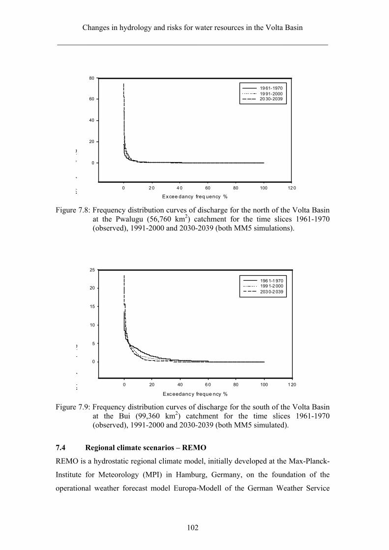
Changes in hydrology and risks for water resources in the Volta Basin
_____________________________________________________________________
102
Excee dancy freq uency %
0 2 0 4 0 60 80 100 12 0
Di
h[
/d]
0
20
40
60
80
19 61-197019 91-200020 30-2039
Figure 7.8: Frequency distribution curves of discharge for the north of the Volta Basin at the Pwalugu (56,760 km2) catchment for the time slices 1961-1970 (observed), 1991-2000 and 2030-2039 (both MM5 simulations).
Exceedancy freque ncy %
0 20 40 6 0 80 100 1 20
Di
h[
/d]
0
5
10
15
20
25
196 1-1 970199 1-2 000203 0-2 039
Figure 7.9: Frequency distribution curves of discharge for the south of the Volta Basin at the Bui (99,360 km2) catchment for the time slices 1961-1970 (observed), 1991-2000 and 2030-2039 (both MM5 simulated).
7.4 Regional climate scenarios – REMO
REMO is a hydrostatic regional climate model, initially developed at the Max-Planck-
Institute for Meteorology (MPI) in Hamburg, Germany, on the foundation of the
operational weather forecast model Europa-Modell of the German Weather Service
Changes in hydrology and risks for water resources in the Volta Basin
_____________________________________________________________________
103
(DWD) (Majewski 1991). According to Jacob et al. (2001) cited in Paeth (2005), the
dynamical kernel is based on primitive equations with temperature, horizontal wind
components, surface pressure, water vapor content and cloud water content as
prognostic variables.
REMO simulations are driven according to Roeckner et al. (2003) by recent
global coupled climate model simulations of ECHAM5/MPI-OM, which are known to
be forced by enhanced greenhouse and sulphate aerosol conditions and are
synonymous with the modeling approaches of the fourth assessment report of the
Intergovernmental Panel on Climate Change (IPCC).
The simulation outputs used for this study are those produced and used in the
GLOWA IMPETUS project whose focus was on western and northern Africa. The
horizontal resolution is 0.5o, equivalent to about 55-km grid spacing at the equator, and
20 hybrid vertical levels are resolved. These levels follow the orography near the
surface and correspond to pressure levels in the upper troposphere (Paeth, 2005).
The global climate model ECHAM4 (Roeckner et al. 1996) was adjusted to
the 0.5o model grid scale of REMO to account for atmospheric processes like deep
convection, cloud formation, convective rainfall, radiation and microphysics from the
sub grid scale of ECHAM4. Similarly, land surface parameters such as soil
characteristics, orography, vegetation, roughness length, and albedo are derived from
the GTOPO30 and NOAA data sets (Hagemann et al. 1999) and partly modified
according to the scenarios of land degradation. Underlying an idealized seasonal cycle
over West Africa, the same daily interpolated surface parameters are prescribed each
year using a model output statistics (MOS) system (Paeth, 2005).
The IMPETUS project made some changes to the default parameter of
REMO to adapt to the tropical-subtropical West African region. The focus is on the
key region of the West African monsoon system of which the Volta Basin is part.
Some results of the adopted REMO correlated well with observed extreme climate
year (Chapter 6). For example, the driest years derived from simulated rainfall were
1981, 1983, 1990, 1992 and 1998, whereas 1979, 1984, 1988, 1989, and 1991 were
characterized by abundant monsoon rainfall. Parker and Alexander (2002) basically
confirm that the CRU time series data set reveals almost the same composite years.
Changes in hydrology and risks for water resources in the Volta Basin
_____________________________________________________________________
104
7.4.1 Highlights of REMO on Volta Basin area
Data on the West African region have large gaps, hence the CRU data set is deficient
in regions with low data coverage. This problem applies to all available gridded
rainfall data sets. REMO, in an attempt to resolve the handicap of data gaps, uses two
statistical post processing steps:
(1) Monthly rainfall is adjusted to the observations by constructing a model output
statistics (MOS) system.
(2) Daily rainfall intensity is corrected from grids by fitting Γ distributions to the
simulated and observed time series, and then taking the ratios between both
distributions as weighting factors in the combined correction algorithm. The
MOS system is defined by von Storch and Zwiers (1999) as stepwise multiple
linear regression analysis.
The MOS-corrected precipitation by the REMO model reveals a good
performance according to Paeth et al. (2005) of the model in terms of the basic
features of African climate, including the complex mid-tropospheric jet and wave
dynamics and the climate seasonality of the Volta Basin area.
Available scenario runs of REMO (Jacob et al. 2001, 2007) in 0.5o resolution
over tropical Africa (Paeth et al. 2005) consider three scenarios of GHG (Figure 7.10)
and emissions and land-cover changes in order to evaluate the range of options given
by different achievements in mitigation policy and to quantify the relative contribution
of land degradation in line with IPCC projections.
The 2007 report of the IPCC lacks new information on the African climate
change but highlights model uncertainties, particularly over tropical Africa. The
inconsistency of different model projections reflects in the low values of the regional
climate change index in Giorgi (2006), which relies on regional temperature and
precipitation changes in the IPCC multi-model ensemble framework. This model
discrepancy clouds the interpretation of the results of uncertain model parameters,
which may impact specifically on the simulation of African climate.
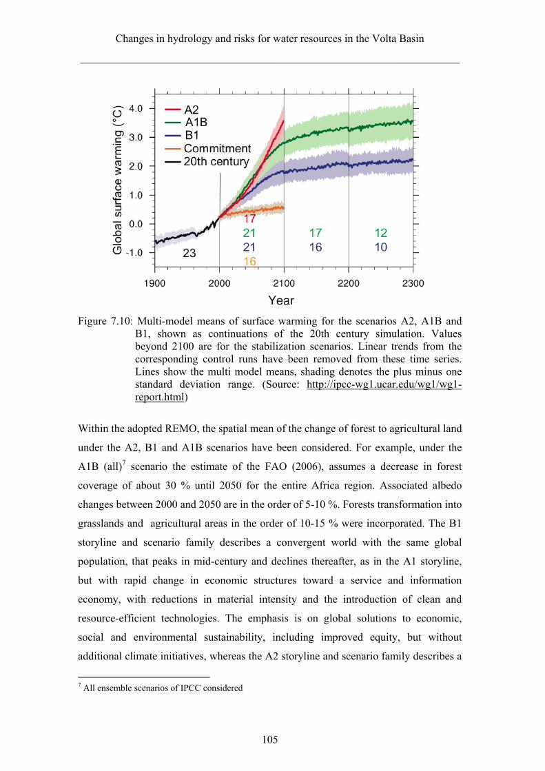
Changes in hydrology and risks for water resources in the Volta Basin
_____________________________________________________________________
105
Figure 7.10: Multi-model means of surface warming for the scenarios A2, A1B and B1, shown as continuations of the 20th century simulation. Values beyond 2100 are for the stabilization scenarios. Linear trends from the corresponding control runs have been removed from these time series. Lines show the multi model means, shading denotes the plus minus one standard deviation range. (Source: http://ipcc-wg1.ucar.edu/wg1/wg1-report.html)
Within the adopted REMO, the spatial mean of the change of forest to agricultural land
under the A2, B1 and A1B scenarios have been considered. For example, under the
A1B (all)7 scenario the estimate of the FAO (2006), assumes a decrease in forest
coverage of about 30 % until 2050 for the entire Africa region. Associated albedo
changes between 2000 and 2050 are in the order of 5-10 %. Forests transformation into
grasslands and agricultural areas in the order of 10-15 % were incorporated. The B1
storyline and scenario family describes a convergent world with the same global
population, that peaks in mid-century and declines thereafter, as in the A1 storyline,
but with rapid change in economic structures toward a service and information
economy, with reductions in material intensity and the introduction of clean and
resource-efficient technologies. The emphasis is on global solutions to economic,
social and environmental sustainability, including improved equity, but without
additional climate initiatives, whereas the A2 storyline and scenario family describes a
7 All ensemble scenarios of IPCC considered
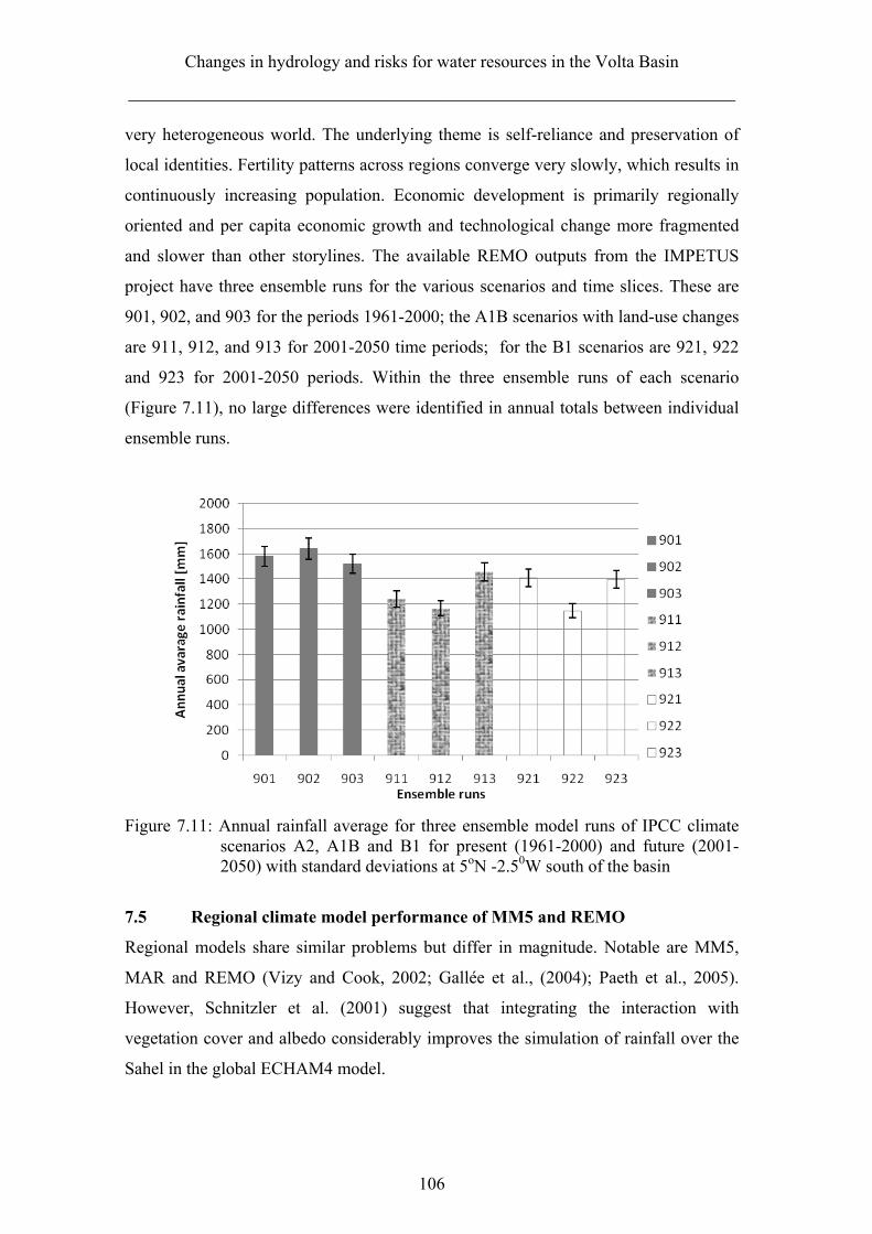
Changes in hydrology and risks for water resources in the Volta Basin
_____________________________________________________________________
106
very heterogeneous world. The underlying theme is self-reliance and preservation of
local identities. Fertility patterns across regions converge very slowly, which results in
continuously increasing population. Economic development is primarily regionally
oriented and per capita economic growth and technological change more fragmented
and slower than other storylines. The available REMO outputs from the IMPETUS
project have three ensemble runs for the various scenarios and time slices. These are
901, 902, and 903 for the periods 1961-2000; the A1B scenarios with land-use changes
are 911, 912, and 913 for 2001-2050 time periods; for the B1 scenarios are 921, 922
and 923 for 2001-2050 periods. Within the three ensemble runs of each scenario
(Figure 7.11), no large differences were identified in annual totals between individual
ensemble runs.
Figure 7.11: Annual rainfall average for three ensemble model runs of IPCC climate scenarios A2, A1B and B1 for present (1961-2000) and future (2001-2050) with standard deviations at 5oN -2.50W south of the basin
7.5 Regional climate model performance of MM5 and REMO
Regional models share similar problems but differ in magnitude. Notable are MM5,
MAR and REMO (Vizy and Cook, 2002; Gallée et al., (2004); Paeth et al., 2005).
However, Schnitzler et al. (2001) suggest that integrating the interaction with
vegetation cover and albedo considerably improves the simulation of rainfall over the
Sahel in the global ECHAM4 model.
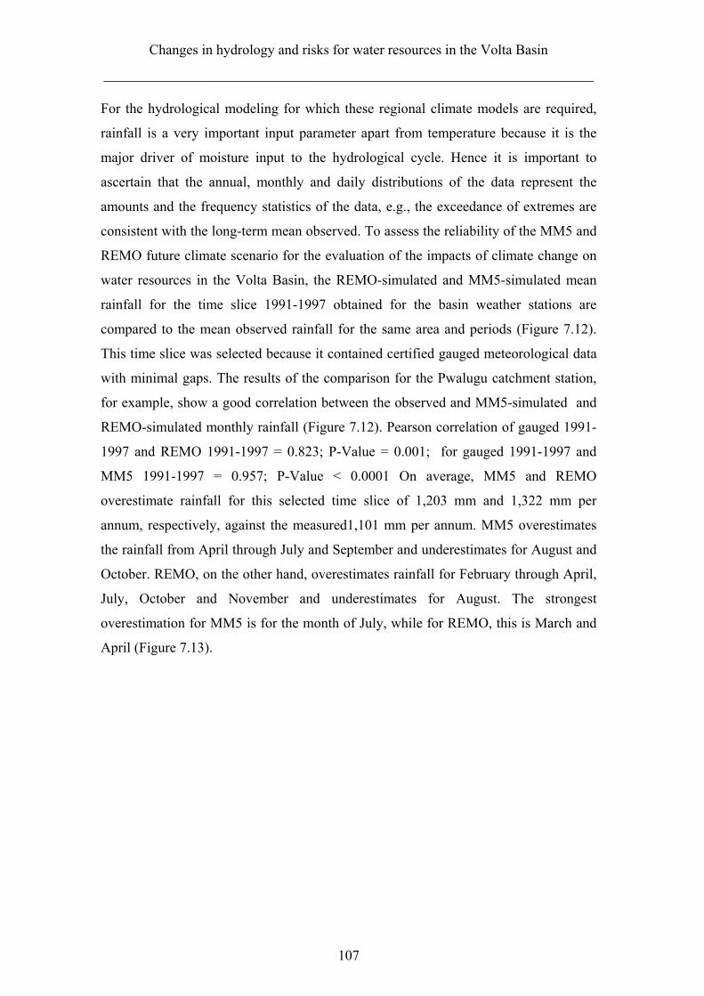
Changes in hydrology and risks for water resources in the Volta Basin
_____________________________________________________________________
107
For the hydrological modeling for which these regional climate models are required,
rainfall is a very important input parameter apart from temperature because it is the
major driver of moisture input to the hydrological cycle. Hence it is important to
ascertain that the annual, monthly and daily distributions of the data represent the
amounts and the frequency statistics of the data, e.g., the exceedance of extremes are
consistent with the long-term mean observed. To assess the reliability of the MM5 and
REMO future climate scenario for the evaluation of the impacts of climate change on
water resources in the Volta Basin, the REMO-simulated and MM5-simulated mean
rainfall for the time slice 1991-1997 obtained for the basin weather stations are
compared to the mean observed rainfall for the same area and periods (Figure 7.12).
This time slice was selected because it contained certified gauged meteorological data
with minimal gaps. The results of the comparison for the Pwalugu catchment station,
for example, show a good correlation between the observed and MM5-simulated and
REMO-simulated monthly rainfall (Figure 7.12). Pearson correlation of gauged 1991-
1997 and REMO 1991-1997 = 0.823; P-Value = 0.001; for gauged 1991-1997 and
MM5 1991-1997 = 0.957; P-Value < 0.0001 On average, MM5 and REMO
overestimate rainfall for this selected time slice of 1,203 mm and 1,322 mm per
annum, respectively, against the measured1,101 mm per annum. MM5 overestimates
the rainfall from April through July and September and underestimates for August and
October. REMO, on the other hand, overestimates rainfall for February through April,
July, October and November and underestimates for August. The strongest
overestimation for MM5 is for the month of July, while for REMO, this is March and
April (Figure 7.13).
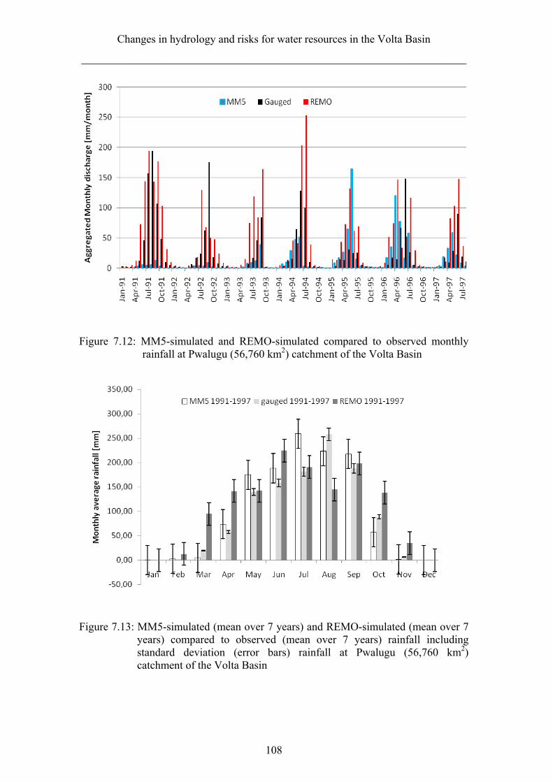
Changes in hydrology and risks for water resources in the Volta Basin
_____________________________________________________________________
108
Figure 7.12: MM5-simulated and REMO-simulated compared to observed monthly rainfall at Pwalugu (56,760 km2) catchment of the Volta Basin
Figure 7.13: MM5-simulated (mean over 7 years) and REMO-simulated (mean over 7 years) compared to observed (mean over 7 years) rainfall including standard deviation (error bars) rainfall at Pwalugu (56,760 km2) catchment of the Volta Basin
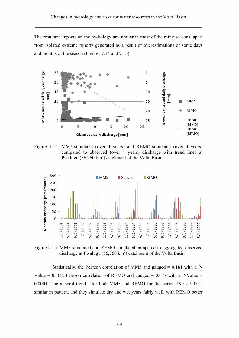
Changes in hydrology and risks for water resources in the Volta Basin
_____________________________________________________________________
109
The resultant impacts on the hydrology are similar in most of the rainy seasons, apart
from isolated extreme runoffs generated as a result of overestimations of some days
and months of the season (Figures 7.14 and 7.15).
Figure 7.14: MM5-simulated (over 4 years) and REMO-simulated (over 4 years) compared to observed (over 4 years) discharge with trend lines at Pwalugu (56,760 km2) catchment of the Volta Basin
Figure 7.15: MM5-simulated and REMO-simulated compared to aggregated observed discharge at Pwalugu (56,760 km2) catchment of the Volta Basin
Statistically, the Pearson correlation of MM5 and gauged = 0.181 with a P-
Value = 0.108; Pearson correlation of REMO and gauged = 0.677 with a P-Value <
0.0001. The general trend for both MM5 and REMO for the period 1991-1997 is
similar in pattern, and they simulate dry and wet years fairly well, with REMO better
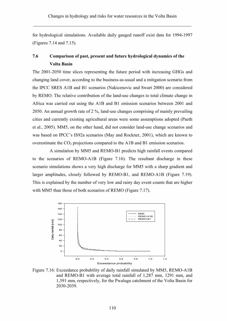
Changes in hydrology and risks for water resources in the Volta Basin
_____________________________________________________________________
110
for hydrological simulations. Available daily gauged runoff exist data for 1994-1997
(Figures 7.14 and 7.15).
7.6 Comparison of past, present and future hydrological dynamics of the
Volta Basin
The 2001-2050 time slices representing the future period with increasing GHGs and
changing land cover, according to the business-as-usual and a mitigation scenario from
the IPCC SRES A1B and B1 scenarios (Nakicenovic and Swart 2000) are considered
by REMO. The relative contribution of the land-use changes to total climate change in
Africa was carried out using the A1B and B1 emission scenarios between 2001 and
2050. An annual growth rate of 2 %, land-use changes comprising of mainly prevailing
cities and currently existing agricultural areas were some assumptions adopted (Paeth
et al., 2005). MM5, on the other hand, did not consider land-use change scenarios and
was based on IPCC’s IS92a scenarios (May and Rockner, 2001), which are known to
overestimate the CO2 projections compared to the A1B and B1 emission scenarios.
A simulation by MM5 and REMO-B1 predicts high rainfall events compared
to the scenarios of REMO-A1B (Figure 7.16). The resultant discharge in these
scenario simulations shows a very high discharge for MM5 with a sharp gradient and
larger amplitudes, closely followed by REMO-B1, and REMO-A1B (Figure 7.19).
This is explained by the number of very low and rainy day event counts that are higher
with MM5 than those of both scenarios of REMO (Figure 7.17).
Exceedance probability
0.0 0.2 0.4 0.6 0.8 1.0 1.2
Dai
ly rai
nfal
l [m
m]
0
20
40
60
80
100
120
140
160
180
MM5REMO-A1BREMO-B1
Figure 7.16: Exceedance probability of daily rainfall simulated by MM5, REMO-A1B and REMO-B1 with average total rainfall of 1,287 mm, 1291 mm, and 1,391 mm, respectively, for the Pwalugu catchment of the Volta Basin for 2030-2039.
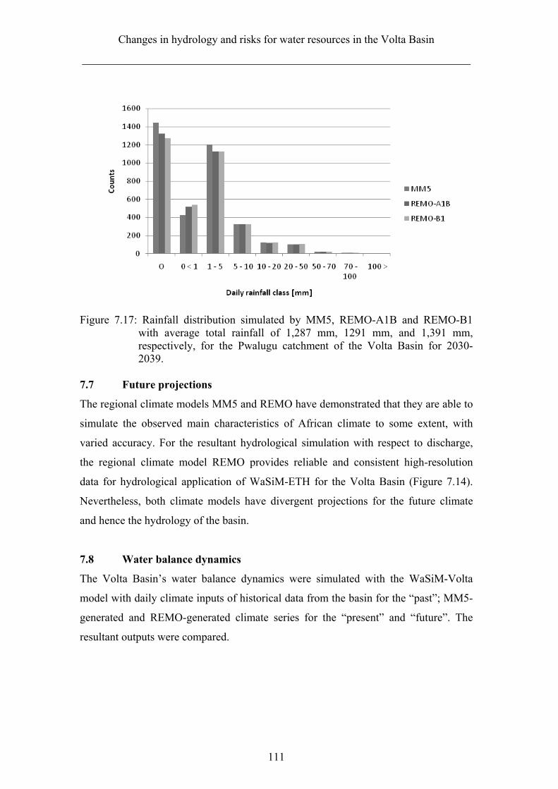
Changes in hydrology and risks for water resources in the Volta Basin
_____________________________________________________________________
111
Figure 7.17: Rainfall distribution simulated by MM5, REMO-A1B and REMO-B1 with average total rainfall of 1,287 mm, 1291 mm, and 1,391 mm, respectively, for the Pwalugu catchment of the Volta Basin for 2030-2039.
7.7 Future projections
The regional climate models MM5 and REMO have demonstrated that they are able to
simulate the observed main characteristics of African climate to some extent, with
varied accuracy. For the resultant hydrological simulation with respect to discharge,
the regional climate model REMO provides reliable and consistent high-resolution
data for hydrological application of WaSiM-ETH for the Volta Basin (Figure 7.14).
Nevertheless, both climate models have divergent projections for the future climate
and hence the hydrology of the basin.
7.8 Water balance dynamics
The Volta Basin’s water balance dynamics were simulated with the WaSiM-Volta
model with daily climate inputs of historical data from the basin for the “past”; MM5-
generated and REMO-generated climate series for the “present” and “future”. The
resultant outputs were compared.
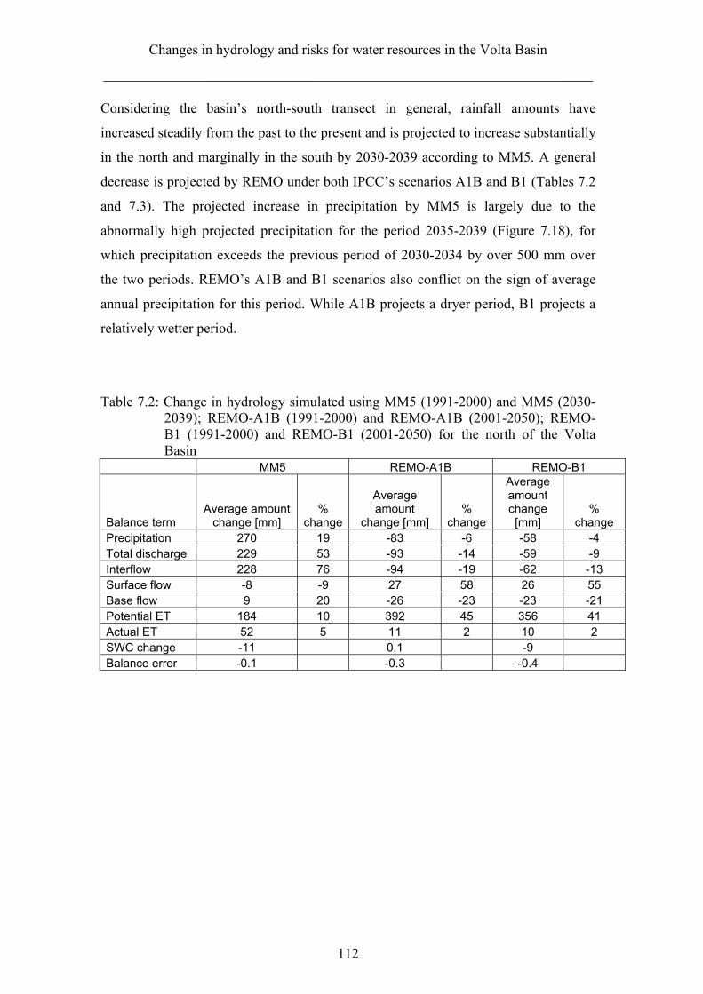
Changes in hydrology and risks for water resources in the Volta Basin
_____________________________________________________________________
112
Considering the basin’s north-south transect in general, rainfall amounts have
increased steadily from the past to the present and is projected to increase substantially
in the north and marginally in the south by 2030-2039 according to MM5. A general
decrease is projected by REMO under both IPCC’s scenarios A1B and B1 (Tables 7.2
and 7.3). The projected increase in precipitation by MM5 is largely due to the
abnormally high projected precipitation for the period 2035-2039 (Figure 7.18), for
which precipitation exceeds the previous period of 2030-2034 by over 500 mm over
the two periods. REMO’s A1B and B1 scenarios also conflict on the sign of average
annual precipitation for this period. While A1B projects a dryer period, B1 projects a
relatively wetter period.
Table 7.2: Change in hydrology simulated using MM5 (1991-2000) and MM5 (2030-2039); REMO-A1B (1991-2000) and REMO-A1B (2001-2050); REMO-B1 (1991-2000) and REMO-B1 (2001-2050) for the north of the Volta Basin
MM5 REMO-A1B REMO-B1
Balance term Average amount
change [mm] %
change
Average amount
change [mm] %
change
Average amount change [mm]
% change
Precipitation 270 19 -83 -6 -58 -4 Total discharge 229 53 -93 -14 -59 -9 Interflow 228 76 -94 -19 -62 -13 Surface flow -8 -9 27 58 26 55 Base flow 9 20 -26 -23 -23 -21 Potential ET 184 10 392 45 356 41 Actual ET 52 5 11 2 10 2 SWC change -11 0.1 -9 Balance error -0.1 -0.3 -0.4
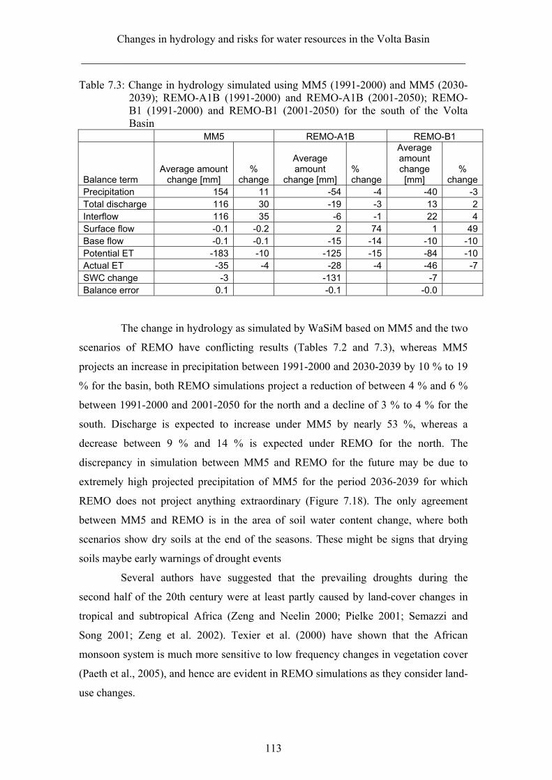
Changes in hydrology and risks for water resources in the Volta Basin
_____________________________________________________________________
113
Table 7.3: Change in hydrology simulated using MM5 (1991-2000) and MM5 (2030-2039); REMO-A1B (1991-2000) and REMO-A1B (2001-2050); REMO-B1 (1991-2000) and REMO-B1 (2001-2050) for the south of the Volta Basin
MM5 REMO-A1B REMO-B1
Balance term Average amount
change [mm] %
change
Average amount
change [mm] % change
Average amount change [mm]
% change
Precipitation 154 11 -54 -4 -40 -3Total discharge 116 30 -19 -3 13 2Interflow 116 35 -6 -1 22 4Surface flow -0.1 -0.2 2 74 1 49Base flow -0.1 -0.1 -15 -14 -10 -10Potential ET -183 -10 -125 -15 -84 -10Actual ET -35 -4 -28 -4 -46 -7SWC change -3 -131 -7 Balance error 0.1 -0.1 -0.0
The change in hydrology as simulated by WaSiM based on MM5 and the two
scenarios of REMO have conflicting results (Tables 7.2 and 7.3), whereas MM5
projects an increase in precipitation between 1991-2000 and 2030-2039 by 10 % to 19
% for the basin, both REMO simulations project a reduction of between 4 % and 6 %
between 1991-2000 and 2001-2050 for the north and a decline of 3 % to 4 % for the
south. Discharge is expected to increase under MM5 by nearly 53 %, whereas a
decrease between 9 % and 14 % is expected under REMO for the north. The
discrepancy in simulation between MM5 and REMO for the future may be due to
extremely high projected precipitation of MM5 for the period 2036-2039 for which
REMO does not project anything extraordinary (Figure 7.18). The only agreement
between MM5 and REMO is in the area of soil water content change, where both
scenarios show dry soils at the end of the seasons. These might be signs that drying
soils maybe early warnings of drought events
Several authors have suggested that the prevailing droughts during the
second half of the 20th century were at least partly caused by land-cover changes in
tropical and subtropical Africa (Zeng and Neelin 2000; Pielke 2001; Semazzi and
Song 2001; Zeng et al. 2002). Texier et al. (2000) have shown that the African
monsoon system is much more sensitive to low frequency changes in vegetation cover
(Paeth et al., 2005), and hence are evident in REMO simulations as they consider land-
use changes.
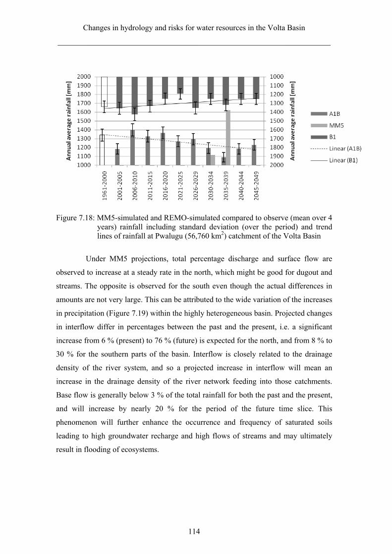
Changes in hydrology and risks for water resources in the Volta Basin
_____________________________________________________________________
114
Figure 7.18: MM5-simulated and REMO-simulated compared to observe (mean over 4 years) rainfall including standard deviation (over the period) and trend lines of rainfall at Pwalugu (56,760 km2) catchment of the Volta Basin
Under MM5 projections, total percentage discharge and surface flow are
observed to increase at a steady rate in the north, which might be good for dugout and
streams. The opposite is observed for the south even though the actual differences in
amounts are not very large. This can be attributed to the wide variation of the increases
in precipitation (Figure 7.19) within the highly heterogeneous basin. Projected changes
in interflow differ in percentages between the past and the present, i.e. a significant
increase from 6 % (present) to 76 % (future) is expected for the north, and from 8 % to
30 % for the southern parts of the basin. Interflow is closely related to the drainage
density of the river system, and so a projected increase in interflow will mean an
increase in the drainage density of the river network feeding into those catchments.
Base flow is generally below 3 % of the total rainfall for both the past and the present,
and will increase by nearly 20 % for the period of the future time slice. This
phenomenon will further enhance the occurrence and frequency of saturated soils
leading to high groundwater recharge and high flows of streams and may ultimately
result in flooding of ecosystems.
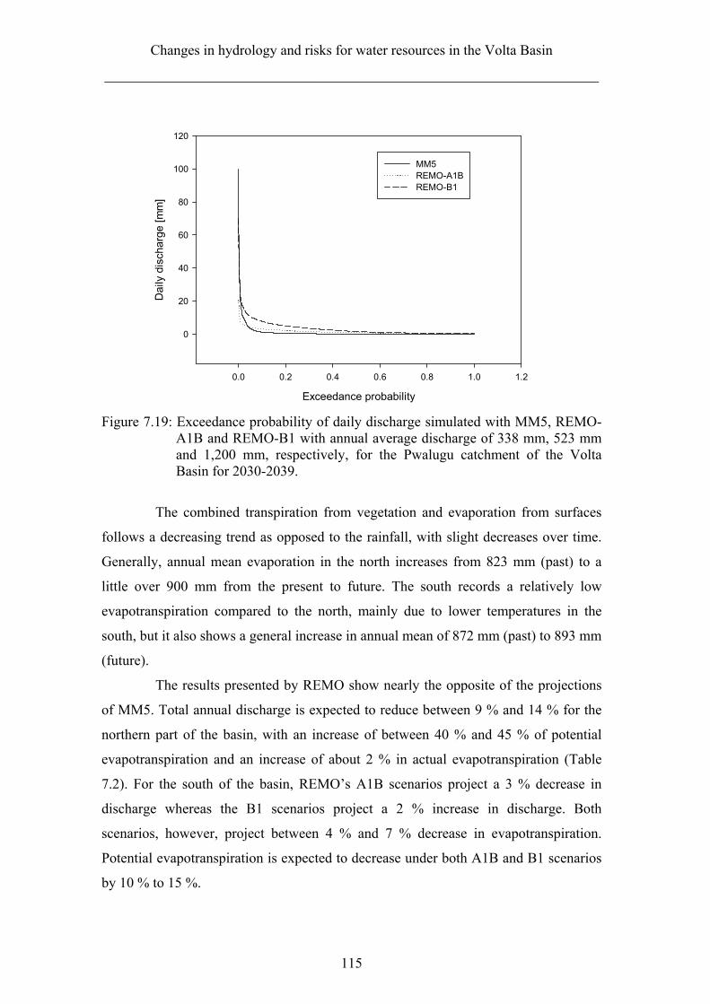
Changes in hydrology and risks for water resources in the Volta Basin
_____________________________________________________________________
115
Exceedance probability
0.0 0.2 0.4 0.6 0.8 1.0 1.2
Dai
ly d
isch
arge
[m
m]
0
20
40
60
80
100
120
MM5REMO-A1BREMO-B1
Figure 7.19: Exceedance probability of daily discharge simulated with MM5, REMO-A1B and REMO-B1 with annual average discharge of 338 mm, 523 mm and 1,200 mm, respectively, for the Pwalugu catchment of the Volta Basin for 2030-2039.
The combined transpiration from vegetation and evaporation from surfaces
follows a decreasing trend as opposed to the rainfall, with slight decreases over time.
Generally, annual mean evaporation in the north increases from 823 mm (past) to a
little over 900 mm from the present to future. The south records a relatively low
evapotranspiration compared to the north, mainly due to lower temperatures in the
south, but it also shows a general increase in annual mean of 872 mm (past) to 893 mm
(future).
The results presented by REMO show nearly the opposite of the projections
of MM5. Total annual discharge is expected to reduce between 9 % and 14 % for the
northern part of the basin, with an increase of between 40 % and 45 % of potential
evapotranspiration and an increase of about 2 % in actual evapotranspiration (Table
7.2). For the south of the basin, REMO’s A1B scenarios project a 3 % decrease in
discharge whereas the B1 scenarios project a 2 % increase in discharge. Both
scenarios, however, project between 4 % and 7 % decrease in evapotranspiration.
Potential evapotranspiration is expected to decrease under both A1B and B1 scenarios
by 10 % to 15 %.
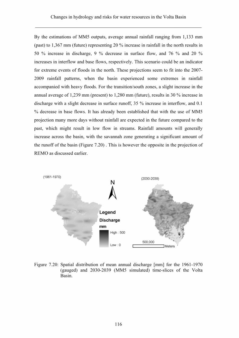
Changes in hydrology and risks for water resources in the Volta Basin
_____________________________________________________________________
116
By the estimations of MM5 outputs, average annual rainfall ranging from 1,133 mm
(past) to 1,367 mm (future) representing 20 % increase in rainfall in the north results in
50 % increase in discharge, 9 % decrease in surface flow, and 76 % and 20 %
increases in interflow and base flows, respectively. This scenario could be an indicator
for extreme events of floods in the north. These projections seem to fit into the 2007-
2009 rainfall patterns, when the basin experienced some extremes in rainfall
accompanied with heavy floods. For the transition/south zones, a slight increase in the
annual average of 1,239 mm (present) to 1,280 mm (future), results in 30 % increase in
discharge with a slight decrease in surface runoff, 35 % increase in interflow, and 0.1
% decrease in base flows. It has already been established that with the use of MM5
projection many more days without rainfall are expected in the future compared to the
past, which might result in low flow in streams. Rainfall amounts will generally
increase across the basin, with the savannah zone generating a significant amount of
the runoff of the basin (Figure 7.20) . This is however the opposite in the projection of
REMO as discussed earlier.
Figure 7.20: Spatial distribution of mean annual discharge [mm] for the 1961-1970 (gauged) and 2030-2039 (MM5 simulated) time-slices of the Volta Basin.
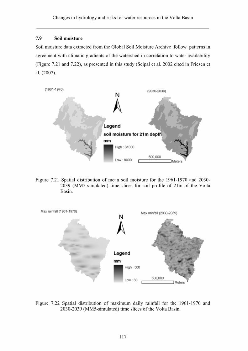
Changes in hydrology and risks for water resources in the Volta Basin
_____________________________________________________________________
117
7.9 Soil moisture
Soil moisture data extracted from the Global Soil Moisture Archive follow patterns in
agreement with climatic gradients of the watershed in correlation to water availability
(Figure 7.21 and 7.22), as presented in this study (Scipal et al. 2002 cited in Friesen et
al. (2007).
Figure 7.21 Spatial distribution of mean soil moisture for the 1961-1970 and 2030-2039 (MM5-simulated) time slices for soil profile of 21m of the Volta Basin.
Figure 7.22 Spatial distribution of maximum daily rainfall for the 1961-1970 and 2030-2039 (MM5-simulated) time slices of the Volta Basin.
Changes in hydrology and risks for water resources in the Volta Basin
_____________________________________________________________________
118
Simulations of soil moisture changes for the three time slices showed that the soil
columns are adequately wet during the rainy season, but are becoming dryer at the end
of the seasons over time. For example, the soil moisture content change will increase
from 9 % from the 1991-2000 time-slice to 12 % of rainfall for the (2030-2039) time-
slice using MM5 simulations. Relatively, soil moisture is higher during the rainy
seasons for the future scenario than for the past (1961-1970). This is due to higher
rainfall amounts attributed to the projected high rainfalls of the 2035-2039 periods.
REMO-A1B projects 2 % decrease in soil water content for the north and 7 % increase
for the south. In contrast, REMO-B1 projects a 9 % increase of soil water content for
the north, and a 6 % increase for the south for the periods 1991-2000 and 2001-2050.
This is mainly due to the temperature and rainfall projections of the scenarios.
7.10 Risk for water resources
The science of the future climate is plagued by uncertainties. For the region of West
Africa, most climate change scenarios predict a decline in precipitation in the range of
0.5-40 % with an average of 10-20 % by 2025. Though other scenarios predict the
contrary, many scenarios portray a more pronounced downtrend in flow regimes. As a
result of the recent major droughts and a number floods with unusual magnitudes,
climate specialists expect exacerbated extreme climate events in some parts of West
Africa (IUCN, 2004). In the wake of all these predictions, it is important to point out
that the climate change scenarios do not consist of definite predictions, but rather
present plausible future conditions. According to Carter and La Rovere (2001), within
climate change studies, high uncertainty requires the use of scenarios that are plausible
but usually have no probability attached to them.
Considering the many possible future scenarios, what matters is the ability to
manage the uncertainty. This includes reducing the current vulnerability of society and
communities to climate variability and extreme events as well as improving and
updating management options to deal with the worst-case scenarios and also take
advantage of opportunities that may arise.
Assessing the risk of climate change, Page and Jones (2001) recommend that
a knowledge of the likelihoods of both climate change and its consequences are
necessary. For example, if greenhouse gas emission scenarios and climate change
Changes in hydrology and risks for water resources in the Volta Basin
_____________________________________________________________________
119
scenarios are plausible with no further likelihood, then the consequences of those
scenarios in terms of impacts have the same limitations. This leads to a growing
cascade of uncertainties associated with a chain of consequences limited by the least
predictable link. A Student’s t-test according to Friesen (2008) on the mean rainfall in
comparison of the periods 1930-1969 and 1970-1995 for the entire basin shows a
significant decline of 28 km3 of rainfall from the former to the latter period with a
confidence interval of 99.9 %.
The water sectors of riparian states have postponed adaptation due to climate
change uncertainty. Although there is wide acceptance that water resources are
sensitive to climate change, managers have delayed accounting for climate change in
their planning until the risks are better known. As generally accepted, the risk of
climate change to a particular activity is a function of probability × hazard, and so,
methods of managing the probabilities are required to go past this blind alley.
Risk is defined as “the objective (mathematical) or subjective (inductive)
probability that the hazard will become an event. Factors (risk factor) can be identified
that modify this probability. Such risk factors are constituted by personal behaviors,
life-styles, cultures, environment factors, and the probability of loss to the elements at
risk as the result of the occurrence, physical and societal consequences of a place in
the community. Risk is the expected number of lives lost, persons injured, damage to
property and disruption of economic activity due to a particular natural phenomenon,
and consequently the product of specific risk and elements at risk” (Journal. of
Prehospital and Disaster Medicine, 2004 cited in Thywisssen, 2006). By this
definition, the basin’s population can be regarded as being highly prone to the risk of
frequent drought according to the projections of REMO and MM5 and some
significant floods based on projected extreme precipitation in the future.
According to Garatwa and Bolli (2002), risk is conventionally expressed by
the equation: Risk = Hazard X Vulnerability. However, the resilience of a society can
help reduce the impact of risk; hence a modified expression as:
–
Changes in hydrology and risks for water resources in the Volta Basin
_____________________________________________________________________
120
A hazard is defined as “A potentially damaging physical event, phenomenon or human
activity that may cause the loss of life or injury, property damage, social and economic
disruption or environmental degradation. Hazards can include latent conditions that
may represent future threats and can have different origins: natural (geological, hydro-
meteorological and biological) or induced by human processes (environmental
degradation and technological hazards). Hazards can be single, sequential or combined
in their origin and effects. Each hazard is characterized by its location, intensity,
frequency and probability.” (UN/ISDR, 2004).
The Volta Basin is prone to various environment-related hazards, most of
which are regarded as natural hazards. Climate change is making the most common
disasters of droughts and floods more likely, as the IPCC warns that global warming
related climate change is likely to lead to more heat waves, droughts, floods and
increased threats to human health. The IPCC Fourth Assessment Report (2007)
elaborated future impacts of climate change on agriculture and many other sectors. In
the Volta Basin region and most especially along the margins of the semi-arid and arid
areas; the length of the growing season and yield potential are expected to decrease
substantially, thus increasing the hazard levels of the basin in many sectors such as
agriculture, food security, etc.
Although no coherent trends are found in the areas around the basin as
reported by Peath et al. (2005), interannual rainfall variability is more pronounced in
the northern Volta (Pwalugu) as revealed by the REMO protections (see Figure 7.23).
The northern part of the basin is most vulnerable to these variations because it has a
monomodal rainfall pattern compared to the south which has relatively higher rainfall
amounts due to its bi-modal rainfall pattern. The SPI analysis conducted on projected
precipitation based on REMO using IPCC’s A1B and B1 scenarios against the base
period of 1961-2000 (Figure 7.23) shows both scenarios agreeing to a general drying
trend for the future. With the exception of B1-scenario-based extreme dry year
projections for 2016 (-2.5) and 2049 (2.1), the A1B scenario generally projects higher
negative SPI values than B1 spanning the entire projection period and more profound
for the period 2019 to 2047.
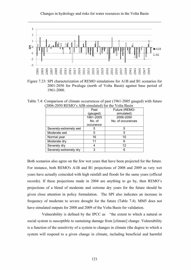
Changes in hydrology and risks for water resources in the Volta Basin
_____________________________________________________________________
121
Figure 7.23: SPI characterization of REMO simulations for A1B and B1 scenarios for 2001-2050 for Pwalugu (north of Volta Basin) against base period of 1961-2000.
Table 7.4: Comparison of climate occurrences of past (1961-2005 gauged) with future (2006-2050 REMO’s AIB-simulated) for the Volta Basin
Past (gauged)
Future (REMO-simulated)
1961-2005 No. of
occurance
2006-2050 No. of occurances
Severely-extremely wet 5 5 Moderate wet 5 5 Normal year 16 10 Moderate dry 11 6 Severely dry 4 12 Severely-extremely dry 3 6
Both scenarios also agree on the few wet years that have been projected for the future.
For instance, both REMO's A1B and B1 projections of 2008 and 2009 as very wet
years have actually coincided with high rainfall and floods for the same years (official
records). If these projections made in 2004 are anything to go by, then REMO’s
projections of a blend of moderate and extreme dry years for the future should be
given close attention in policy formulation. The SPI also indicates an increase in
frequency of moderate to severe drought for the future (Table 7.4). MM5 does not
have simulated outputs for 2008 and 2009 of the Volta Basin for validation.
Vulnerability is defined by the IPCC as “the extent to which a natural or
social system is susceptible to sustaining damage from [climate] change. Vulnerability
is a function of the sensitivity of a system to changes in climate (the degree to which a
system will respond to a given change in climate, including beneficial and harmful
Changes in hydrology and risks for water resources in the Volta Basin
_____________________________________________________________________
122
effects), adaptive capacity (the degree to which adjustments in practices, processes, or
structures can moderate or offset the potential for damage or take advantage of
opportunities created by a given change in climate), and the degree of exposure of the
system to climatic hazards” (IPCC, 2001). Rockström and Falkenmark (2000) and
Friesen (2008) have noted that agricultural productivity within the basin is highly
dependent on available soil moisture, also termed “blue water”. In this light, the IUCN
describes West Africa as among the most vulnerable regions with respect to climate
change worldwide. The region is known not to be sensitized adequately to the
predicted impacts of climate change so as to take actions in preparedness to cope with
climate challenges. For example, the UNFCCC reports that in the Volta Basin region
yields from rainfed agriculture could be reduced by up to 50 % by 2020. With
agriculture being key to the development of the riparian states, losses of between 2 and
7 % of GDP are expected by the year 2100. In the area of water resources availability
and management, the basin countries cannot be said to be doing any better. The Water
Poverty Index (WPI) used to monitor development in water resources management
credits most of the riparian states with a WPI of approximately 45 of 100 according to
calculations over many years (Sullivan et al. 2001 cited in Eguavoen (2007)); this
exacerbates the already gloomy situation.
The 2007 human development report of the UN Development Program
(UNDP) described vulnerability in the context of climate change as "an inability to
manage risk without being forced to make choices that compromise human well-being
over time."
Resilience is also defined as “the capacity of a system, community or society
potentially exposed to hazards to adapt by resisting or changing in order to reach and
maintain an acceptable level of functioning and structure. This is determined by the
degree to which the social system is capable of organizing itself to increase its capacity
for learning from past disasters for better future protection and to improve risk
reduction measures” (UN/ISDR, 2004). Resilience is one component that directly
reduces risk. In the Volta Basin, building resilience to climate change through adaptive
processes seem to be on the low priority end, as ad hoc relief measures are employed
for addressing the effects of hazards without recourse to future occurrences.
Changes in hydrology and risks for water resources in the Volta Basin
_____________________________________________________________________
123
In summary, the hazard factors regarding the risk of failing water resources are
increasing in the basin, thus increasing the vulnerability of the population to climate
shocks. With little or no resilience building, the risks for inhabitants of the Volta Basin
threaten life and property, and thus need urgent attention.
7.11 Impacts of climate change on Volta Basin water resources
The impacts of climate-related factors on water resources and their management poses
threats in many sectors of society. It is projected that though a general increase in
rainfall is proposed by some regional models, the increases in low flow events in
streams will eventually increase the occurrence of droughts which usually have severe
consequences for most sectors, particularly agriculture, energy, and domestic water for
most communities of the basin who depend on streams for their water needs.
On the other hand, according to the IPCC (2007), increases in the frequency
and intensity of rainfall may increase the occurrence of flooding due to heavy rainfall
events. Apart from the devastating consequences of flood to the vulnerable
communities of the basin, groundwater recharge may also be affected, because more
flash flows will be generated to the detriment of percolation; with such reductions, the
availability of groundwater for drinking water and dry season irrigation could be at
risk in some parts of the basin.
Water resources management has its own handicaps, but in addition to the
typical problems of water management, climate change introduces another dimension
and additional element of uncertainty about future water resource management, which
need holistic approaches to overcome. In policies for water resources management,
strategies will need to be developed to match continued evolution of the complex
dynamics of water availability to address the issues. Implementation of adaptation
measures, such as water conservation, reduction in water demand and use, new
strategies for droughts and floods resistant farming, and the application of appropriate
and pragmatic management practices will play a crucial role in the determination and
reduction of the impacts of climate change on water resources of the Volta Basin.
Though regional models such as MM5 and REMO do not agree on the
direction of changes within the Volta Basin, there is consensus that the impacts of
Changes in hydrology and risks for water resources in the Volta Basin
_____________________________________________________________________
124
climate change on water resources could pose huge challenges to the uses and
management of these resources.
7.12 Comparison of study results with previous studies
The contradicting future simulated annual discharge and changes in hydrology
obtained with the use of the regional models MM5 and REMO in this study for the
Volta Basin are similar to what has been obtained in other investigations. Jung (2006)
coupled WaSiM version 1 with MM5 and reported that for the future of 2030-2039, an
average of 5 % increase in rainfall was expected with a wide variation of 20 % - 50 %
between the Sahel and the Guinea Coast. In her report, no changes are expected for
interflow for the future in the entire basin. Surface runoff is projected to increase by 17
% resulting in an overall increase in discharge. Actual evapotranspiration will increase
for the future Wagner (2008) agrees with results of Jung (2006).
Obuobie (2009) in an assessment of the impacts of climate changes on the
hydrology of the White Volta of the Volta Basin using the soil-water assessment tool-
SWAT with MM5 inputs and the climate generator LARS-WG for future scenarios,
projected increases in total discharge and groundwater recharge for the periods 2030-
2039 and 2070-2099. He reported 29 % increase in subsurface flow due to an increase
in discharge and surface runoff. Rainfall is expected to increase by 6 % with MM5
projections and 3 % with LARS-WG, resulting in 3 % rise in discharge, 15 % increase
in surface runoff and 4 % decrease in base flow. The discharge simulated with MM5
projections gives an increment of 33 % by 2030-2039.
It is worth noting that overland flow due to saturation excess is an important
mechanism for runoff generation under natural vegetation, in particular at the bottom
of slopes (see Hiepe, 2008). The lateral movement of water in the shallow subsurface
that is usually termed interflow complicates the computation of surface runoff due to
the interaction between surface and subsurface flows.
Most reports on climate and hydrology of the Volta Basin project increases in
rainfall and discharge. However, reports of the IMPETUS project, which used the
REMO model based on the IPCC’s A1B and B1 second report emissions forcing
scenarios incorporating land-use changes, forecast declines in rainfall and discharge
for Benin, which is very similar in climate and hydrology to the Volta Basin and
Changes in hydrology and risks for water resources in the Volta Basin
_____________________________________________________________________
125
shares the same micro-climate of West Africa. In the case of temperature, all
projections of all studies for the basin agree on an increasing trend. For example, the
results of the business as usual scenario, combined with IPCC Scenarios A1B and B2
through the year 2045 on plausible scenarios of future economic, demographic, and
climate developments, effects of land-use and land-cover change, climate change, and
demographic development on water availability and water demand for Benin (West
Africa) reveal a significant decrease in water availability (surface water and
groundwater) due to a decrease in rainfall and a significant increase in
evapotranspiration. Although total water consumption increases strongly, it represents
only about 0.5% of the yearly renewable water resources (Christoph et al., 2008). In
the quantification of runoff processes and sheet and rill erosion in the Upper Ouémé
River catchment in central Benin, Hiepe (2008) found that changes in climate variables
led to decreases in sediment yield of 5 to 14 % in 2001-2025 and 17 to 24 % in 2026-
2050, which could be attributed to increasing surface flow due to land-use changes and
high rainfall events. Combined scenarios showed the dominance of land-use change
leading to changes in mean sediment yield of -2 to +31 % in 2001-2025.
Conclusions and outlook
_____________________________________________________________________
126
8 CONCLUSIONS AND OUTLOOK
8.1 Conclusions
The conclusions reached using WaSiM model agree with many in the natural science
community that global warming is occurring as a result of anthropogenic activities
which are causing climate change. It is therefore important to monitor the entire chain
of water availability and use in order to understand and address the negative effects of
climate change.
Implementing adaptation measures such as water conservation and reduction
in water demand and use, new strategies for drought and flood-resistant farming, and
the application of appropriate and pragmatic management practices will play a crucial
role in the determination and reduction of the impacts of climate change on water
resources of the Volta Basin.
The calibrated hydrological model WaSiM-Volta showed a good performance
in the representation of the hydrology of the Volta Basin, and was thus suitable for the
study of the hydrological dynamics of the basin. The calibration of WaSiM and the
validation processes for the two sub-catchments of the basin at Pwalugu in the north
and Bui in the south revealed that credible meteorological conditions, most especially
rainfall and temperature, are critical in the realistic simulation of the resultant
hydrological processes of the basin. The calibration period was 1968-1971 with a model
warm-up period of 1961-1967 in daily, weekly and monthly aggregations. Validation
was carried out for the period 1994-2001 for both catchments. The highest aggregation
(monthly) exhibited the best calibration results with a coefficient of determination (R2)
of 0.98 between simulated and observed discharge and R2=0.96 and R2= 0.87 for the
weekly and daily, respectively. The Willmott index of agreement was 0.93, 0.96, and
0.99 for the daily, weekly and monthly calibration, respectively, showing a good
correlation between simulated and observed discharge. However, the model generally
underestimated some peak flow that could be due to missing or inaccurate data, but
simulated low and normal flow fairly well. The Nash-Sutcliffe efficiency index was
0.94, 0.83 and 0.74 for the monthly, weekly and daily discharge respectively.
The classification and evaluation of different SPI drought coverage according
to WaSiM simulation resulted in percent areal distribution of drought intensities for
Conclusions and outlook
_____________________________________________________________________
127
selected threshold levels and frequency analysis in percent areal distribution to
determine return periods of drought intensities. From the 1980s, frequent dry periods of
shorter intervals occurred between 1983 and 2001. The basin experienced at least four
moderately dry years covering 50 % of the area. Simulations of changes in soil moisture
for the three time slices showed that the soil profile is adequately wet during the wet
season and dryer in the dry season. Simulations indicate changes in soil moisture
declining from 9 % from the 1991-2000 periods to 12 % of rainfall for 2030- 2039. It
also estimates higher soil moisture during the rainy season for the “future” scenario than
for the “past” (1961 to 1970) due to “future” higher rainfall amounts.
The results from the comparison of the Volta Basin water balance dynamics,
simulated with WaSiM-Volta model, using historical climate data from the basin for the
“past”, and MM5- generated climate series for the “present” and the “future” with even
durations of 10 years show that in the basin in general, from the north to the south,
rainfall has increased steadily from the past to the present, and it is projected to increase
substantially in the north and marginally in the south from 2030 to 2039. The WaSiM
simulation using REMO data show a different trend of decrease in rainfall, and
consequently decreases in almost all the discharge components of the periods 1961-
2000 and 2001-2050.
Analysis of climate data in the basin indicates that the months in which
precipitation exceeds evapotranspiration are usually June, July, August and September.
A comparison of wet and dry years shows that the ratio of direct runoff and base flow is
at an average of 30 %, being high in the wet years with a sharp decline in the dry years.
It is observed that total percentage discharge and surface flow have increased in the
north, which might be good for dugouts and streams; the opposite is true for the south.
The probability of daily average discharge falling below 1 mm is expected to
increase from 0.47 in the “past” to 0.75 for the “future” time slice of 2030 to 2039 in the
south of the basin, thus increasing the frequency of low flow occurrences. The annual
recharge for the Volta River System ranges from 13 % to 16 % of the mean annual
precipitation, and annual rainfall amounts from the simulations show an increase of
between 11 % and 20 % for the highly heterogeneous basin. It is important to note,
however, that REMO gives exactly opposite outputs to the scenario outputs of MM5.
Conclusions and outlook
_____________________________________________________________________
128
The calibration and validation results demonstrate that the model performed credibly in
mimicking the daily, weekly and monthly discharge, surface runoff, interflow and base
flow, soil moisture and evapotranspiration comparable to those of other numerous
studies conducted within the basin at different times.
Modeling in general has many constraints, but is a good tool in understanding
those underlying processes that are sometimes nearly impossible to measure. On the
whole, the results from WaSiM-Volta show the capability of simulating and shedding
light on impacts of climate variations on the hydrology of the Volta Basin.
Temperature has been rising over the years and causes increases in
evapotranspiration, and hence annulling any surplus that might have been gained with
the increase in rainfall amounts. With the increase in population and demand for food
and increasing water use, coupled with poor water management practices and increasing
risk of climate change, resultant impacts could reach undefined proportions for the
inhabitants of the Volta Basin. The frequency of droughts has already been established
to have increased over the last decades, and with the increase in high-intensity
precipitation, flood occurrences are also eminent. The time has come to include the
hazards with discovered trends into policy making for the riparian states of the Volta
Basin to reduce the impacts of climate variability and increase the coping capacity of
the communities. It is also now evident that, irrespective of the measures and policies
aimed at mitigating the impacts of climate change, there is an urgent need to build
capacity to reduce vulnerability to climate variability and change.
8.2 Outlook
Accurate estimation of the surface and subsurface hydrology is very important for
sustainable management programs of water resources of any basin. However, this can
only be achieved with equally accurate meteorological information. It is therefore
advisable to verify as much as possible climatic data such as temperature, rainfall,
humidity, wind speed, etc. It must be noted that gauged discharge is also estimated and
suffer from some uncertainties. Care must be taken when simulations, which are
estimates, are manipulated to fit observed measurements.
The hydrology of a basin is not only dependent on climate inputs, but also on
spatial variables such as land use/land cover and topography among others. Future
Conclusions and outlook
_____________________________________________________________________
129
scenarios were conducted with current land-use / land-cover maps, and this could lead
to errors in projections. Projected simulations would be desirable if varied simulation
of land use / land cover, and soil texture scenarios are modeled alongside the hydrology
to access all possible scenarios to account for the feedback that might exist.
It is assumed that there are to some extent links between sea surface
temperature and the rainfall distribution and pattern of the West African monsoon.
Further studies concerning the influence of the sea surface temperatures on the rainfall
of the Volta Basin are needed. The results fed into WaSiM simulations may give an
improved view of the dynamics of the water of the Basin and increase the predictability
of the hydrological impact on various scenarios.
References
_____________________________________________________________________
130
9 REFERENCES
Acheampong SY (1996) Geochemical evolution of the shallow groundwater system in the Southern Voltaian Sedimentary Basin of Ghana. PhD dissertation, University of Nevada, Reno
Adger WN, Brooks N, Kelly M, Bentham G, Agnew M, and Eriksen S (2004) New indicators of vulnerability and adaptive capacity, Tyndall Final project Report P IT1.11: July 2001 TO June 2003
Agyare W (2004) Soil characterization and modelling of spatial distribution of saturated hydraulic conductivity at two sites in the Volta basin of Ghana. Doctoral thesis, University of Bonn, Bonn, http://www.zef.de/fileadmin/ webfiles/downloads/zefc_ecology_development/ecol_dev_17_text.pdf
Altman D (1991) Practical Statistics for Medical Research. Chapman & Hall, London. Altman DG and Bland JM (1983) Measurement in medicine: the analysis of method
comparison studies. Statistician. 32, pp. 307-317 Amani A (2001) Assessment of precipitation and resources variability across the
Sahelian region, in: Gash, J.H.C., Odada, E.O., Oyebande, L. and Schulz, R.E.; Report of the International Workshop on Africa’s Water Resources, Nairobi, 26-30 October 1999 (BAHC)
Amisigo BA (2005) Modelling riverflow in the Volta Basin of West Africa: A data-driven framework. PhD Thesis. Ecology and Development Series No. 34. ZEF Bonn. Cuvillier Verlag, Göttingen, http://www.glowa-volta.de/fileadmin/ template/ Glowa/ Downloads/Amisigo_doc_thesis _2006 .pdf
Anderson M P and Woessner WW (1992) Applied Groundwater Modelling. Academic Press, San Diego
Andreini M, van de Giesen N, van Edig A, Fosu M, and Andah W (2000) Volta Basin Water Balance. ZEF – Discussion Papers on Development Policy, No. 21, ZEF, Bonn
Arnold JG, Sirinivasan R, Muttiah RS, and William JR (1998) Large area hydrologic modelling and assessment, Part 1: Model development. Journal of the American water resources association, 34(1)
ASCE Task Committee on Definition of Criteria for Evaluation of Watershed Models of the Watershed Management, Irrigation, and Drainage Division (ASCE), (1993) Criteria for evaluation of watershed models. J. Irrig. Drain. Eng., 1193, 429–442
Aspden RM (2005) Agreement between two experimental measures or between experiment and theory. Journal of Biomechanics, 38, pp. 2136-2137.
Barry B, Obuobie E, Andreini M, Andah W, and Pluquet M (2005) The Volta river basin. Comprehensive assessment of water management in agriculture. Comparative study of river basin development and management. Draft http://www.iwmi.cgiar.org/assessment/research_projects/river_basin_development_and_management/projects_locations/volta_river_burkina_faso_ghana.htm
Beven K and Feyen J (2002) The future of distributed modelling. Hydrological Processes, 16, 169-172
Bevington P R and Robinson D K (1992) Data reduction and error analysis for the physical sciences. New York, McGraw-Hill
Bhalme H N and Mooley D A (1980) Large-scale drought flood and monsoon circulation. Mon. Weather Rev.: 108, 1197 - 1211
References
_____________________________________________________________________
131
Birikundavyi S, Labib R, Trung H T, and Rousselle J (2002) Performance of neural networks in daily streamflow forecasting. J. Hydrol. Eng., 75, 392–398
Bland J M and Altman D G (1996) Transforming data. BMJ 312(7033): 770 Bland JM and Altman D G (1995. Comparing two methods of clinical measurement: a
personal history. Int J Epidemiol 24 Suppl 1: S7-14 Bland JM and Altman DG (1986) Statistical methods for assessing agreement between
two methods of clinical measurement. The Lancet Blöschl,G. (1996): Scale and scaling in hydrology. Dissertation, TU Wien, 1-22. Broekhuyse J (1983) Transformatie van Mossi land. Koninklijk Instituut voor de
Tropen (Amsterdam): 168p Brown JD and Heuvelink GBM (2005) Assessing Uncertainty Propagation Through
Physically based Models of Soil Water Flow and Solute Transport. Anderson, M.G. & J.J. McDonnell (Eds) Encyclopaedia of Hydrological Sciences. Wiley Blackwell. 3456 p
Brutsaert W (1982) Evaporation into the atmosphere: theory, history and applications.
Reidel, Dordrecht.
Busche H, Hiepe C, Diekkrüger B (2005) Modelling the effects of land use and climate change on hydrology and soil erosion in a sub-humid African Catchment. Proceedings of the 3rd International SWAT Conference 2005, pp434-443Carter TR and La Rovere EL (2001) Developing and applying scenarios. In: McCarthy, J.J., Canziani, O.F., Leary, N.A., Dokken, D.J. and White, K.S. (eds.) Climate Change 2001: Impacts, Adaptation, and Vulnerability, Contribution of Working Group II to the Third Assessment Report of the Intergovernmental Panel on Climate Change, Cambridge University Press, Cambridge, 145–190
Castaing C, Billa M, Milesi JP, and Thieblemont D (2003) Notice explicative de la carte géologique et minière du Burkina Faso 1:1 000 000. Ministère des Mines, des Carrières et de l'Energie, Ouagadougou
Chekol DA (2006) Modelling of Hydrology and Soil Erosion of Upper Awash River Basin. PhD Thesis, University of Bonn: 233pp
Christoph M, Fink A, Diekkrüger B, Giertz S, Reichert B and Speth P (2008) Water SA Vol. 34 No. 4 (Special HELP edition) 2008
CLIVAR - Project (2004) National Research Council (U.S.). Committee to Review the U.S. Climate Variability and Predictability Review of the U.S. CLIVAR Project Office. Washington, DC, National Academies Press
Darko PK and Krasny J (2003) Regional transmissivity distribution and groundwater potential in hard rocks of Ghana, in Krasny, Hrkal, Bruthans (Edts): Groundwater in fractured rocks, 45-46, Prag
David S, Bowles P, and Enda O'Connell (1991) Recent advances in the modelling of hydrologic systems, North Atlantic Treaty Organization. Scientific Affairs Division, Springer, 667 pages
Diamond J (2005) Collapse: how societies choose to fail or succeed Viking: New York Downer C W and Ogden F L (2004) “GSSHA: Model to simulate diverse stream flow
producing processes.” J. Hydrol. Eng., 93,161–174 Dugue P (1989) Possibilités et limites de l’intensification des systemes de cultures
vivriers en zone Soudano-Sahelienne: le cas du Yatenga (Burkina Faso). Collection Documents Systèmes Agraires No. 9(DSA/CIRAD, Montpellier, France)
References
_____________________________________________________________________
132
Eguavoen I (2007) Now you have a new pump, you have to manage it. Household water management, water rights and institutional change in Northern Ghana. Doctoral thesis, Institute of Social Anthropology, Philosophical Faculty, Albert-Magnus Universität. Cologne/ Germany, http://www.glowa-volta.de/fileadmin/template/Glowa/Downloads/Eguavoen_phdThesis.pdf
Elston J (1983) "Climate." Potential productivity of field crops under different environments International Rice Research Institute (IRRI) Manila, Philippines: 3-14
Erpul G, Norton L D, and Gabriels D (2003) Sediment transport from interrill areas under wind-driven rain. J. Hydrol., 276, 184–197
FAO (1971-81) Soil Map of the World. United Nations Food and Agriculture Organization, UNESCO, Paris
FAO (1995) Digital soil map of the world and derived soil properties (CDROM) food and Agriculture Organization of the United Nations. FAO
FAO (2005) Irrigation in Africa in Figures. FAO Water Report No 29. Rome. 74pp FAO (2006) Food and Africulture Organization, Global forest resources assessment
2005. Progress towards sustainable forest management. FAO Forestry Paper, 147, 348pp
Friesen J (2002) Spatio-temporal rainfall patterns in Northern Ghana. Diplom thesis, Geographic Institute, Rheinische Friedrich-Wilhelm-Universität, Bonn
Friesen J, Andreini M, Andah W, Amisigo B, and van de Giesen N (2005) Storage capacity and long term water balance of the Volta Basin, West Africa. p. 138-145. IAHS-AISH publication 296
Friesen J, Winsemius H C, Beck R, Scipal K, Wagner W, and van de Giesen N (2007) Spatial and seasonal patterns of diurnal differences in ERS Scatterometer soil moisture data in the Volta Basin, West Africa. p. 47-55. IAHS-AISH Publication 316
Friesen JC (2008) Regional vegetation water effects on satellite soil moisture estimations for West Africa. Doctoral thesis, Rheinische Friedrich Wilhelms Universität, Bonn/ Germany, http://www.glowa-volta.de/fileadmin/template/ Glowa/Downloads/EDS_63__Jan_Friesen.pdf
Gallée H Moufouma-Okia W Bechtold P Brasseur O Dupays I Marbaix P Messager C Ramel R and Lebel T (2004) A high-resolution simulation of a West African rainy season using a regional climate mode. J. Geophys. Res. 109, 10.1029/2003JD004020
Garatwa W and Bollin C (2002) Disaster Risk Management Working Concept. Eschborn, Deutsche Gesellschaft für Technische Zusammenarbeit (GTZ), http://www2.gtz.de/dokumente/bib/02-5001.pdf>, last accessed 2/06/2009
Giertz S (2004) Analyse der hydrologischen Prozesse in den sub-humiden Tropen Westafrikas unter besonderer Berücksichtigung der Landnutzung am Beispiel des Aguima-Einzugsgebietes in Benin; PhD thesis; University Bonn, http://hss.ulb.uni-bonn.de/diss_online/ math_nat_fak/2004/giertz_simone /giertz.htm
Giorgi F (2006) Climate change hot-spots. Geophys. Res. Let., 33, doi:10.1029/2006GL025734
Green Cross International (2001) Trans-boundary Basin Sub-Projects: The Volta River Basin. Website: <www.gci.ch/Green- crossPrograms/ waterres/pdf/WFP_ Volta>
Green W H and Ampt G A (1911) Studies on soil physics: The flow of air and water through soils. Journal of agricultural science, 4, 1-24
References
_____________________________________________________________________
133
Grell GA, Dudhia J, and Stauffer DR (1995) A description of the Fifth-Generation Penn State /NCAR Mesoscale Model (MM5). Tech. rept.
Gurtz J, Zappa M, Jasper K, Lang H, Verbunt M, Badoux A, and Vitvar T (2003) A comparative study in modelling runoff and its components in two mountainous catchment. Hydrological Processes, 17, 297-311
Hagemann S, Botzet M, Dümenil L and Machenhauer B (1999) Derivation of global GCM boundary conditions from 1 km land use satellite data. Max-Planck-Inst. f. Meteor., Report No. 289, Hamburg
Hayward D and Oguntoyinbo J (1987) Climatology of West Africa. Hutchindson. Henriques AG and Santos MJJ (1999) Regional Drought Distribution Model. Phys.
Chem. Earth (B) No.1-2:19-22 Herschy RW (1978) Hydrometry: principles and practices. Wiley & Sons, Chichester,
127-130 Herschy RW (1999) Hydrometry—Principles and Practices, Journal of Hydrology 222,
191–194 Hewitson BC and Crane RG (2006), Consensus between GCM climate change
projections with empirical downscaling: Precipitation downscaling over South Africa, Int. J. Climatol. 26: 1315–1337 (2006)
Hiepe C (2008) Soil degradation by water erosion in a sub-humid West-African catchment: a modelling approach considering land use and climate change in Benin, Doctoral thesis, Rheinische Friedrich Wilhelms Universität, Bonn/ Germany, http://hss.ulb.uni-bonn.de/diss_online/math_nat_fak/2008/hiepe_ claudia/ index.htm
Hiepe C and Diekkrüger B (2007) Modelling soil erosion in a sub- humid tropical environment at the regional scale considering land use and climate change. Book of abstracts, 4th International SWAT conference, UNESCO-IHE Institute for Water Education, Delft, The Netherlands. July 4-6, 2007
Hisdal H and Tallaksen L M (2000) Assessment of the Regional Impact of Droughts in Europe. Drought Event Definition Technical Report to the ARIDE project No. 6
Hodnett M G and Tomasella J (2002) Marked differences between van Genuchten soil water-retention parameters for temperate and tropical soils: a new water retention pedo-transfer functions developed for tropical soils. Geoderma, 108, 155-180.
Hulme M, Doherty R, Ngara T, New M, and Lister D (2001) African climate IAHS Publ., No. 252: p. 307-314
International Institute of Environment and Development - IIED (1992) Annual report IPCC 2007 Climate Change (2007) The Physical Science Basis. Contribution of
working group I to the fourth Assessment Report of the Intergovernmental Panel on Climate Change [Solomon, S., D. Qin, M. Manning, Z. Chen, M. Marquis, K.B. Averyt
IPCC (2001) Climate Change (2001) Synthesis Report. A Contribution of Working Groups I, II, and III to the Third Assessment Report of the intergovernmental Panel on Climate Change. Watson, R.T. et al. (Eds.). Cambridge University Press, Cambridge, New York, p. 398
IPCC (2001) Climate Change -The Scientific Basis, J. T. Houghton et al., (Eds) Cambridge Univ. Press, Cambridge
IPCC (2007) IPCC Fourth Assessment Report: Climate Change 2007. Geneva, Switzerland
References
_____________________________________________________________________
134
IPCC 2007 Climate Change 2007 Impacts, Adaptation, and Vulnerability. Contribution of Working Group II to the Fourth Assessment Report of the Intergovernmental Panel on Climate Change [Parry, Martin L., Canziani, Osvaldo F., Palutikof, Jean P., van der Linden, Paul J., and Hanson, Clair E. (eds.)]. Cambridge University Press, Cambridge, United Kingdom, 1000 pp
IPCC AR4 (2005) are available (https://esg.llnl.gov:8443/home/publicHomePage.do) IUCN (2004) Reducing West Africa’s Vulnerability to Climate Impacts on Water
Resources, Wet lands and Desertification: Elements for a Regional Strategy for Preparedness and Adaptation. Niasse, Madiodio, Afouda, Abel, Amani, Abou.(Eds.) Gland, Switzerland and Cambridge, UK.xviii+66pp
Jacob D Van den Hurk BJJM Andrae U Elgered G Fortelius C Graham LP Jackson SD Karstens U Koepken C Lindau R Podzun R Rockel B Rubel F Sass BH Smith R and Yang X (2001) A comprehensive model intercomparison study investigating the water budget during the PIDCAP period. Meteorol. Atmos. Phys. 77, 19-44
Jacob D, Bärring L, Christensen OB, Christensen JH, de Castro M, Déqué M, Giorgi F, Hagemann S, Hirschi M, Jones R, Kjellström E, Lenderink G, Rockel B, Sánchez ES, Schär C, Seneviratne S, Somot S, van Ulden A, van den Hurk B (2007) An intercomparison of regional climate models for Europe: model performance in present-day climate. Climatic Change, 81:31-52
Jacob D Van den Hurk BJJM Andrae U Elgered G Fortelius C Graham LP Jackson SD Karstens U Koepken C Lindau R Podzun R Rockel B Rubel F Sass BH Smith R and Yang X (2001) A comprehensive model intercomparison study investigating the water budget during the PIDCAP period. Meteorol. Atmos. Phys. 77, 19-44
Jain S, Storm B, Bathurst J, Refsgaard J, and Singh R (1992) Application of the SHE to catchments in India Part 2. Field experiments and simulation studies with the SHE on the Kolar subcatchment of the Narmand river. Journal of Hydrology 140, 25–47
Jarque CM and Bera AK (1980) Efficient tests for normality, heteroskedasticity, and serial independence of regression residuals. Economic Letter 6, 255–259
Jasper K, Gurtz J, and Lang H (2002) Advances flood forecasting in Alpine watersheds by coupling meteorological observations and forecasts with a distributed hydrological model. Journal of Hydrology, 267, 40-52
Jenkins G S, Gaye A T, and Sylla B (2005) Late 20th century attribution of drying trends in the Sahel from the Regional Climate Model (RegCM3), Geophys. Res. Lett., 32, L22705, doi:10.1029/2005GL024225
Jenkins G S, Kamga A, Adamou G, Diedhiou A, Morris V, and Joseph E (2002) Summary of the Workshop on Modeling the West African Climate System with Global and Regional Scale Climate Models: Relevance to Understanding Climate Variability, Land-Use, and Climate Change, BAMS, 583-595, 2002
Johnson M S, Coon W, Mehta V, Steenhuis T, Brooke E, and Boll J (2003) Applications of two hydrologic models with different runoff mechanisms to a hillslope dominated watershed in the northeastern U.S.: A comparison of HSPF and SMR. J. Hydrol., 284, 57–76
Jung G (2006) Regional Climate Change and the Impact on Hydrology in the Volta Basin of West Africa. Dissertation Garmisch-Partenkirchen, Germany
Kalin L, Govindaraju R S, and Hantush M M (2003) Effect of geomorphological resolution on modelling of runoff hydrograph and sedimentograph over small watersheds. J. Hydrol., 276, 89–111
References
_____________________________________________________________________
135
Kalin L, Govindaraju R S, and Hantush M M (2003) Effect of geomorphological resolution on modeling of runoff hydrograph and sedimentograph over small watersheds. J. Hydrol., 276, 89–111
Kasei C N (1988) The Physical environment of semi-arid Ghana. In: Challenges in Dryland Agriculture. A global perspective (ed). P. W. Unger. T. V. Sneed, W. R. Jordan and R. Jensen. : 350 – 354
Kasei C N and Sallah P Y K (1993) Drought evasion in crop production under a monomodal rainfall pattern. Paper presented at the third workshop on improving farming systems in the Savannah Zone of Ghana. April 17 - 29
Kasei C N, Mercer-Quarshie H, and Sallah P YK (1995) Identifying probable dry periods in maize production under a monomodal rainfall regime in Northern Ghana. 29 May - 2nd June 1995, IITA Proceedings of a Regional Maize Workshop A WECAMAN/IITA publication March, 1997
Kasei R (2006) Determination of Sensible Heat Flux from Large Aperture Scintillometer Measurements in the Volta Basin of Ghana. M.Phil Thesis. University of Cape Coast/ Wageningen University, Ghana, 119
Kilgore JL (1997) Development and evaluation of a GIS based spatially distributed unit hydrograph model. MSc. Thesis, Virginia Polytechnic Institute and State University
Krause J (2003) Inverse hydrologische Modellierung für das Einzugsgebiet der Ammer mittels WaSiM-ETH und PEST, University of Trier, master thesis (in german), 135 p
Krause P, Boyle DP, and Base F (2005) Comparison of different efficiency criteria for hydrological model assessment. Advances in Geosciences, 5,89–97
Kunstmann H and Jung G (2005) Impact of regional climate change on water availability in the Volta basin of West Africa. In: Regional Hydrological Impacts of Climatic Variability and Change. IAHS Publ. 295
LeBarbé L and Lebel T (1997) Rainfall climatology of the HAPEX-Sahel rgion during the years 1950-1990; Journal of Hydrology; Vol. 188-189: pp. 43–73
LeCompte FJ, Iannarilli MR, Hess GA, Freund DL, McMaster DB and Nichols JE (1994) Rice, Proceedings of the IRIS Specialty Group on Targets, Backgrounds, and Discrimination, Monterey, CA, February 1, 1994
Leemhuis C (2005) The Impact of El Niño Southern Oscillation Events on Water Resource Availability in Central Sulawesi, Indonesia: A hydrological modelling approach. Dissertation. Göttingen, Germany
Legates D R and McCabe G J (1999) Evaluating the use of goodness-of-fit measures in hydrologic and hydroclimatic model validation. Water Resources Research, 35, 233-241
Leube A and Hirdes W (1986) The Birimian Supergroup of Ghana: Depositional environment, Structural Development and Conceptual Model of an Early Proterozoic Suite. Hannover, Federal Ministry for Economic Cooperation, p. 259
M. Tignor and H.L. Miller (Eds.)]. Cambridge University Press, Cambridge, United Kingdom and New York, NY, USA, 996pp
Maidment DR (1992) Handbook of Hydrology. McGraw-Hill, Inc Majewski D (1991) The Europa-Modell of the Deutscher Wetterdienst. Seminar
Proceedings ECMWF 2, 147-191 Mamdouh S (2002) Hydrology and water resources of Africa, Springer, 659 Pages Martin N (2005) Development of a water balance for the Atankwidi catchment, West
Africa – A case study of groundwater recharge in a semi-arid climate. PhD
References
_____________________________________________________________________
136
thesis; Georg- August-Universität Göttingen, Germany, http://www.glowa-volta.de/fileadmin/template/Glowa/Downloads/thesis_martin.pdf
Martin N and Giesen N van de (2005) Spatial distribution of groundwater production and development potential in the Volta river basin of Ghana and Burkina Faso. Water International, 30(2), 239–249,
May W and Röckner E (2001) A time-slice experiment with the ECHAM4 AGCM at high resolution: the impact of horizontal resolution on annual mean climate change; Climate Dynamics; Vol. 17: pp. 407–420
McKee T B, Doesken N J and Kleist J (1993) The Relationship of Drought Frequency and Duration to Time Scales. 8th Conference on Applied Climatology, Anaheim, CA, USA,: 179-184
Mearns LO, Giorgi F, Whetton P, Pabon D, Hulme M, and Lal M (2004) Guidelines for use of climate scenarios developed from regional climate model experiments, Tech. rep., Data Distribution Centre of the IPCC
Merz R and Bloschl G (2004) Regionalization of catchment model parameters. J. Hydrol., 287, 95–123
Monteith JL (1975) Vegetation and the atmosphere, vol.1:Principles Academic Press. Moussa R (2008) Significance of the Nash-Sutcliffe efficiency measure for linear rise
and exponential recession in event based flood modelling. Geophysical Research Abstracts, Vol. 10, EGU2008-A-08369, 2008 SRef-ID: 1607-7962/gra/EGU2008-A-08369 EGU General Assembly 2008 http://www.fao.org/DOCREP/005/Y3948F/y3948f00.htm#toc
Nakicenovic N and Swart R (Eds.) (2000) Emission Scenarios. 2000. Special Report of the Intergovernmental Panel on Climate Change. Cambridge University Press, U.K., 570pp
Nash J E and Sutcliffe J V (1970) River flow forecasting through conceptunal models. Journal of Hydrology, 10, 282-290
Nathan C (1970) Framework for River Basin Planning. Ghana Sector Studies. Interim Report for Ministry of Finance and Economic Planning
Nicholson S (1994) Recent rainfall fluctuations in Africa and their relationship to past conditions over the continent. The Holocene 4, 2, 121-131
Nicholson S (2005) On the question of the ‘‘recovery’’ of the rains in the West African Sahel. Journal of Arid Environments 63: 615-641
Nicholson SE (1979) Revised rainfall series for the West African subtropics. Monthly Weather Review, 107, 620-623
Nicholson SE (1983) Recent rainfall fluctuations in Africa and their relationship to past conditions over the continent. The Holocene 4, 2, 121-131
Nicholson SE (1983) Sub-Saharan Rainfall in the Years 1976-1980: Evidence of Continued Drought. Monthly Weather Review, 111, 8, 1646-1654
Nicholson SE (1985) Sub-Saharan rainfall 1981: - 1984:. Journal of Climate and Applied Meteorology, 24, 1388-1391
Nicholson SE (1993) An Overview of African Rainfall Fluctuations of the Last Decade. Journal of Climate, V6, 7. 1463-1466
Nicholson SE (1993) An Overview of African Rainfall Fluctuations of the Last Decade. Journal of Climate, V6, 7. 1463-1466
Nicholson SE (2007) A revised picture of the structure of the "monsoon" and land ITCZ over West Africa. Submitted to the Bulletin of the American Meteorological Society
References
_____________________________________________________________________
137
Nicholson SE and Palao IM (1993) A Re-Evaluation of Rainfall Variability in the Sahel .Part I. Characteristics of Rainfall Fluctuations. Int. Journal of Climatology, 13, 371-389
Nicholson SE, Ba MB and Kim JY (1996) Rainfall in the Sahel during 1994 Journal of Climate, 9, July, 1673-1676
Nicholson SE, Marengo JA, Kim J, Lare AR, Galle S, Kerr YH. (1997) A daily resolution evapoclimatonomy model applied to surface water balance calculations at the HAPEX-Sahel supersites. Journal of Hydrology, 188-189 (1-4), pp. 946-964
Nicholson SE, Tchayi MGN and Bertrand JJ (1996) The Diurnal and Seasonal Cycles of Desert Dust over Africa North of the Equator . Journal of Applied Meteorology, 36, 868-882
Niehoff D (2001) Modellierung des Einflusses der Landnutzung auf die Hochwasserentstehung in der mesoskala. Dissertation, Universität Potsdam,
Obuobie E (2008) Estimation of groundwater recharge in the context of future climate change in the White Volta River Basin. Doctoral thesis, Rheinische Friedrich Wilhelms Universität, Bonn/ Germany, http://www.glowa-volta.de/fileadmin/template/Glowa/ Downloads/Obuobie_No_62_full.pdf
Oguntunde P G (2004) Evapotranspiration and complimentarity relations in the water balance of the Volta Basin: Field measurements and GIS-based regional estimates;. Ecology and Development Series No. 22, Cuvillier Verlag Göttingen, http://www.zef.de/fileadmin/webfiles/ downloads/zefc_ecology_ development/ecol_dev_22_text.pdf
Oguntunde PG, Friesen J, Giesen N van de, Hubert HG, and Savenije HHG (2006) Hydroclimatology of the Volta River Basin in West Africa: Trends and variability from 1901 to 2002 Physics and Chemistry of the Earth 31 (2006) 1180–1188 Oke TR (1987) Boundary Layer Climates. Routledge.
Oladipo E O (1985) A comparative performance analysis of three meteorological drought indices. 5, 655 - 664
Opoku-Ankomah Y (1998) Volta Basin System Surface Water Resources in Water Resources Management Study. Information Building Block. Part II, Vol. 2. Ministry of Works and Housing. Accra, Ghana
Opoku-Ankomah Y (2000) Impacts of Potential Climate Change on River Discharge in Climate Change Vulnerability and Adaptation Assessment on Water Resources of Ghana. Water Research Institute (CSIR), Accra, Ghana
Paeth H and Thamm HP (2007) Regional modelling of future African climate including greenhouse warming and land degradation. – In: Climatic Change 83, 401-427
Paeth H Born K Podzun R and Jacob D (2005) Regional dynamic downscaling over West Africa: Model evaluation and comparison of wet and dry years. Meteorol. Z., 14, 349-367
Page CM and Jones RN (2001) Coupling a climate scenario generator with impact models using OzClim. In: Proceedings of the MODSIM Congress, Canberra
Palmer W C (1965) Meteorological drought.U. S. Weather Bureau Res. paper No. 45 Parker DE and Alexander LV (2002) Global and regional climate in 2001. Weather
57,328-340 Pearson K (1900) On the criterion that a given system of deviations from the probable
in the case of a correlated system of variables is such that it can be reasonably supposed to have arisen from random sampling. Philosophical Magazine Series 5, 50:157-175, 1900
References
_____________________________________________________________________
138
Peschke G (1989) Localizing groups with action, Publicacions Matemátiques, Vol 33 (1989), 227-234
Pielke RA (2001) Influence of the spatial distribution of vegetation and soils on the prediction of cumulus convective rainfall. Rev. Geophysics 39, 151-177
Pierce DA and Schafer DW (1986) Residuals in Generalized Linear Models, Journal of the American Statistical Association, 81, 977-986
PPMED (1987) Ministry of Finance and Economic Planning (Accra, Ghana) Rassmusson EM, Dickinson RE, Kutzbach JE and Cleaveland MK (1993) Climatology.
In: Maidment, D.R. ed. Handbook of Hydrology. McGraw-Hill, Inc., New York, NY, 2.1-2.44
Refsgaard A and Storm B (1996) Distributed physically-based modelling of the entire land phase of the hydrological cycle. In: Abbott, M. B. and Refsgaard, J. C. (Eds.): Distributed hydrological modelling. Kluwer Academic Publisher, Dordrecht, 55-69
Rockström J and Falkenmark M (2000) Semiarid crop production from a hydrological perspective: gap between potential and actual yields. Critical Reviews in Plant Sciences, 19: 319–346
Rodier J (1964) Régimes Hydrologiques de l’Afrique Noire à Ouest du Congo. ORSTOM, Paris
Roeckner E Arpe K Bengtsson L Christoph M Claussen M Dümenil L Esch M Giorgetta M Schlese U and Schulzweida U (1996) The atmospheric general circulation model ECHAM-4: Model description and simulation of present-day climate. Max-Planck-Inst. f. Meteor., Report No. 218. Hamburg
Roeckner E et al. (2003) The atmospheric general circulation model ECHAM 5. PARTI: Model description. MPI Report, 349, 127pp
Sastry PSN (1976) Climate and crop planning with particular reference to rainfall. In: Climate and Rice, Proceedings of the Symposium, International Rice Research Institute, 1976, pp. 5163
Schellekens J (2000) Hydrological processes in a humid tropical rainforest: a combined experimental and modelling approach. Dissertation, Vrije Universiteit Amsterdam, 7-9
Schnitzler K-G Knorr W Latif M Bader J and Zeng N (2001) Vegetation feedback on Sahelian rainfall variability in a coupled climate land-vegetation model. Max-Planck-Inst. f. Meteor., Report No. 329, Hambrug
Schulla J (1997) Hydrologische Modellierung von Fliessgebieten zur Abschatzung der Folgen van Klimaandenmgen. Dissertation ETH 12018, Verlag Geographisches Institut ETH Zurich
Schulla J and Jasper K (1999) Model description WaSiM-ETH, ETH, Zürich, http://www.igm.uni-hohenheim.de/cms/fileadmin/documents/Project Docs/ OtherDocuments/wasim00english.pdf”.
Schulla J and Jasper K (2000) Model Description WASIM-ETH (Water Balance Simulation Model ETH), ETH-Zurich, Zurich.
Scipal K, Wagner W, Trommler M, and Naumann K (2002) The global soil moisture archive 1992-2000 from ERS scatterometer data: First results. p. 1399-1401. International Geoscience and Remote Sensing Symposium (IGARSS)
Semazzi HF M and Sun L (1995) On the modulation of the Sahelian summer rainfall by bottom topography. AMS 75th anniversary. Global Climate Change Conference. Houston Texas January 1995
Semazzi FHM and Song Y (2001) A GCM study of climate change induced by deforestation in Africa. Climate Res. 17, 169-182
References
_____________________________________________________________________
139
Servant E, Patureel I, Kouamé B, Ouédraogo T, Boyer JF, Lubés-Neil H, Fritsch JM, Masson JM and Marieu B (1998) Identification, characterization and consequences of a hydrological variability in West and Central Africa; In: Proc. Int. Conf. at Abidjan on the variability of water resources in Africa in the 20th century, IAHS Publ., No. 252: p. 307-314
Shahin M (2002) Hydrology and water resources of Africa. Water Science and Technology library. Kluwer academic publisher, Dordrecht, Netherlands. 659p
Singh V P and Woolhiser DA (2002) Mathematical modelling of watershed hydrology. Journal of Hydrologic Engineering 7:270-292
Stadler C (2002) Anwendung des hydrologischen flächendifferenzierten Wasserhaushaltmodell WaSIM-ETH im Einzugsgebiet der Mangfall. Diplom thesis, Universität Augsburg, Augsburg
Sintondji L (2005) Modelling of process rainfall-runoff in the Upper Quémé catchmentarea (Terou) in a context of climate change: extrapolation from the local scale to a regional scale. PhD Thesis. Shaker Verlag, Aachen, Germany
Storch H and Stehr N (2006) Anthropogenic climate change - a reason for concern since the 18th century and earlier. Geogr. Ann., 88 A (2): 107–113
Sullivan CA (2001) The potential for calculating a meaniful water poverty index. Water Int 26: 471-480
Texier D de Noblet N and Braconnot P (2000) Sensitivity of the African and Asian monsoons to mid-holocene insolation and data-inferred surface changes. J. Cimate 13, 164-181
Thorpe AJ (2005) Climate change prediction. A challenging scientific problem. A paper produced on behalf of the Institute of Physics, London, UK
Thywissen K (2006), Components of Risk-A comparative glossary. UNU Institute for Environment and Human Security (UNU-EHS), Germany
Troch PA, Paniconi C, and McLaughlin (2003) catchment-scale hydrological modelling and data assimilation, Preface/Advances in Water Resources 26:131-135
UN/ISDR (2004) Living with Risk: A global review of disaster reduction initiatives. 2004 Version, Volume II Annexes. Geneva
UNEP- United Nations Environment Programme (2008) UNEP Year Book: an overview of our changing environment 2008
UNEP -United Nations Environmental Protection (2001) Proposal for a Project Development and Preparation Facility (PDF) Block B Grant: Benin, Burkina Faso, Côte d’Ivoire, Ghana, Mali, Togo. Integrated Management of the Volta River Basin. Available at http://www.gefweb.org/COUNCIL/GEF_C15/GEF_ C15_Inf.13/ PDFBVOLTAFINALSENT GEFSEC.pdf. Accessed in November 2004
UNESCO (1978) Some Suggestions on Teachings about Human Rights, UNESCO, Paris
Van Belle G (2008) Statistical rules of thumb, second edition, Jon Wiley & sons, Inc. Hoboken, New Jersey
van Edig A, van de Giesen N, Andreini M, and Laube W (2001) Institutional and legal aspects of the (transboundary) Water Resources Commission in Ghana. Wasserkonflikte in der Dritten Welt, 18
Van Genuchten M TH (1980) A closed form equation for predicting the hydraulic condictivity of unsaturated soils. Soil Science Society, 44, 892-898
References
_____________________________________________________________________
140
Verbunt M, Gurtz J, Jasper K, Lang H, Warmerdam P, and Zappa M (2003) The hydrological role of snow and glaciers in alpine river basins and the distributed modelling. Journal of Hydrology, 282, 36-55
Vizy EK and Cook KH (2002) Development and application of a meso-scale climate model for the tropics: Influence of sea surface temperature anomalies on the West African monsoon. J.Geophys. Res. 107, 10.1029/2001JD000686
von Storch H and FW Zwiers (1999) Statistical analysis in climate research. Cambridge University Press, Cambridge, UK, 484pp
Wagner S (2008) Water Balance in a Poorly Gauged Basin in West Africa Using Atmospheric Modelling and Remote Sensing Information. Doctoral Thesis, Intitut für Wasserbau, Universität Stuttgart, Germany
Westgard JO and Hunt .R (1973) Use and interpretation of common statistical tests in method-comparison studies. Clinical Chemistry, 19, 49-57
Willmott CJ (1981) On the validation of models. Physical Geography 2, 184-194. Willmott CJ (1984) On the evaluation of model performance in physical geography. in
Spatial Statistics and Models, G.L. Gaile, and C.J. Willmott (Editors). D. Reidel, Dordrecht, 443-460
World Bank (1992) World Development Report 1992: Development and the Environment. Oxford University Press, Oxford, for World Bank, Washington DC. 308 pp
Xu C (1999) Operational testing of a water balance model for predicting climate change impacts, Jou Agricultural and Forest Meteorology, 98-99, 295-304
Yildiz O (2007) Investigating frequency and spatial characteristics of drought in the central anatolian region, Turkey. International Congress on River Basin Management.http://www.dsi.gov.tr/english/congress2007/chapter_3/91.pdf
Zeng N and Neelin JD (2000) The role of vegetation-climate interaction and interannual variability in shaping the African Savanna. J. Climate, 13, 2665-2670
Zeng N Hales K and Neelin JD (2002) Nonlinear dynamics in a coupled vegetation atmosphere system and implications for desert-forest gradient. J. Climate 15, 3474-3487
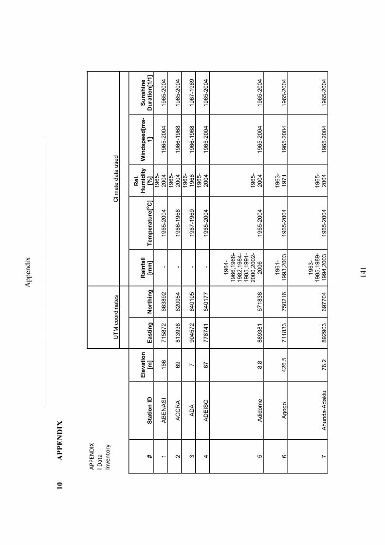
App
endi
x
____
____
____
____
____
____
____
____
____
____
____
____
____
____
____
____
____
_
141
10
AP
PE
ND
IX
APPEN
DIX
I Data
Inventory
U
TM
coo
rdin
ates
C
limat
e da
ta u
sed
# S
tati
on
ID
E
leva
tio
n
[m]
Eas
tin
g
No
rth
ing
R
ain
fall
[mm
] T
emp
erat
ure
[oC
]
Rel
. H
um
idit
y [%
] W
ind
spee
d[m
s-1]
S
un
shin
e D
ura
tio
n[1
/1]
1 A
BE
NA
SI
166
7158
72
663
892
-
1965
-200
4 19
65-
200
4
196
5-20
04
196
5-20
04
2 A
CC
RA
69
81
393
8
620
054
-
19
66-
1968
19
65-
200
4
196
6-19
68
196
5-20
04
3 A
DA
7
904
572
64
010
5
-
196
7-19
69
196
6-19
68
19
66-
1968
19
67-
1969
4 A
DE
ISO
67
77
874
1
640
177
-
19
65-
2004
19
65-
200
4
196
5-20
04
196
5-20
04
5 A
did
ome
8.
8
889
381
67
183
8
196
4-19
66,
1968
-19
82,
1984
-19
85,
1991
-20
00,
2002
-20
06
19
65-
2004
19
65-
200
4
196
5-20
04
196
5-20
04
6 A
gog
o
426.
5
711
833
75
021
6
196
1-19
93,
2003
19
65-
2004
19
63-
197
1
196
5-20
04
196
5-20
04
7 A
hun
da-A
dakl
u 76
.2
892
903
69
770
4
196
3-19
85,
1989
-19
94,
2003
19
65-
2004
19
65-
200
4
196
5-20
04
196
5-20
04
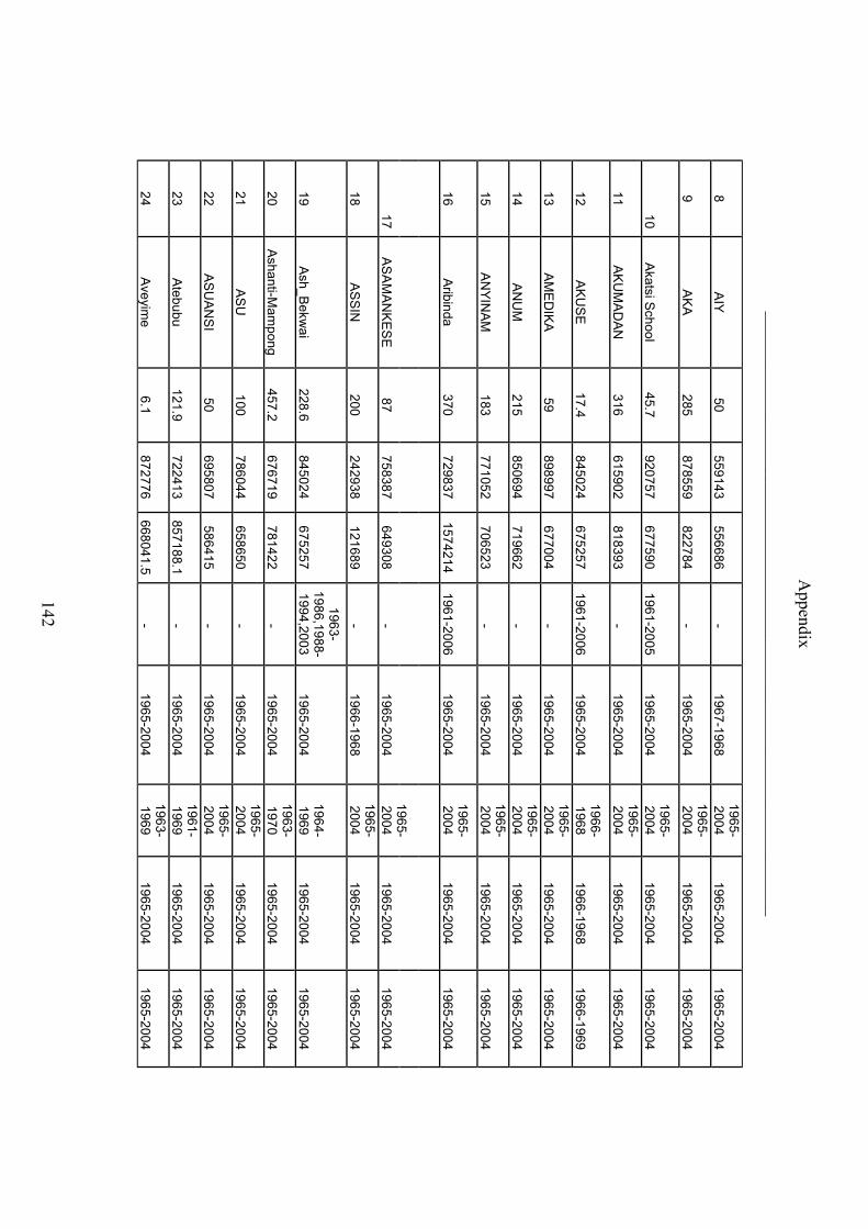
Appendix
_____________________________________________________________________
142
8 A
IY
50
55914
3
55668
6
- 196
7-1968
196
5-200
4
1965-20
04
1965-20
04
9 A
KA
285
878559 822784
- 1965-2004
1965-
2004
196
5-2004
196
5-2004
10A
katsi Schoo
l 45.7
920
757
677
590
196
1-2005
196
5-2004
196
5-200
4
1965-20
04
1965-20
04
11
AK
UM
AD
AN
316
615
902
818
393
-
1965-20
04
1965-
2004
196
5-2004
196
5-2004
12
AK
US
E
17.4
84502
4
67525
7
1961-20
06
1965-20
04
1966-
1968
196
6-1968
196
6-1969
13
AM
ED
IKA
59
898
997
677
004
-
1965-20
04
1965-
2004
196
5-2004
196
5-2004
14
AN
UM
215
850
694
719
662
-
1965-20
04
1965-
2004
196
5-2004
196
5-2004
15
AN
YIN
AM
183
771
052
706
523
-
1965-20
04
1965-
2004
196
5-2004
196
5-2004
16
Aribin
da
370
72983
7
15742
14
1961-20
06
1965-20
04
1965-
2004
196
5-2004
196
5-2004
AS
AM
AN
KE
SE
87
758387 649
308 -
1965-2004 196
5-200
4
1965-20
04
1965-20
04
17
18 A
SS
IN
200 242938
121689
- 1966-1968
1965-
2004
196
5-2004
196
5-2004
19
Ash_B
ekwa
i 228.6
845
024
675
257
1963-
1986,19
88-199
4,2003
196
5-2004
196
4-196
9
1965-20
04
1965-20
04
20
Ashanti-M
amp
ong
457.2
67671
9
78142
2
- 196
5-2004
196
3-197
0
1965-20
04
1965-20
04
21
AS
U
100
78604
4
65865
0
- 196
5-2004
196
5-200
4
1965-20
04
1965-20
04
22
AS
UA
NS
I 50
695
807
586
415
-
1965-20
04
1965-
2004
196
5-2004
196
5-2004
23
Atebub
u
121.9
72241
3
85718
8.1 -
1965-20
04
1961-
1969
196
5-2004
196
5-2004
24
Ave
yime
6.1
872
776
668
041.5
- 196
5-2004
196
3-196
9
1965-20
04
1965-20
04
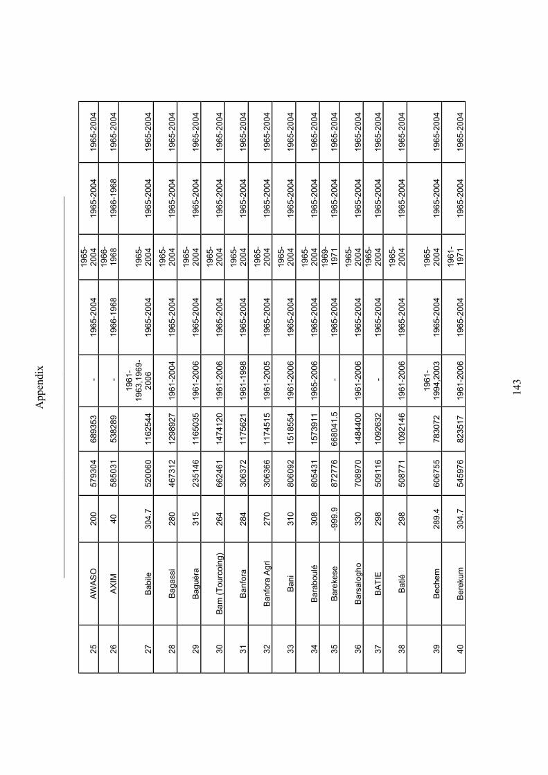
App
endi
x
____
____
____
____
____
____
____
____
____
____
____
____
____
____
____
____
____
_
143
25
AW
AS
O
200
57
930
4
689
353
-
19
65-
2004
19
65-
200
4
196
5-20
04
196
5-20
04
26
AX
IM
40
585
031
53
828
9
-
196
6-19
68
196
6-19
68
19
66-
1968
19
65-
2004
27
Bab
ile
304.
7
520
060
11
625
44
196
1-19
63,
1969
-20
06
19
65-
2004
19
65-
200
4
196
5-20
04
196
5-20
04
28
Bag
assi
28
0
467
312
12
989
27
196
1-20
04
196
5-20
04
196
5-20
04
19
65-
2004
19
65-
2004
29
Bag
uér
a
315
23
514
6
116
5035
19
61-
2006
19
65-
2004
19
65-
200
4
196
5-20
04
196
5-20
04
30
Bam
(T
ourc
oin
g)
264
66
246
1
147
4120
19
61-
2006
19
65-
2004
19
65-
200
4
196
5-20
04
196
5-20
04
31
Ban
fora
28
4
306
372
11
756
21
196
1-19
98
196
5-20
04
196
5-20
04
19
65-
2004
19
65-
2004
32
Ban
fora
Agr
i 27
0
306
366
11
745
15
196
1-20
05
196
5-20
04
196
5-20
04
19
65-
2004
19
65-
2004
33
Ban
i 31
0
806
092
15
185
54
196
1-20
06
196
5-20
04
196
5-20
04
19
65-
2004
19
65-
2004
34
Bar
abou
lé
308
80
543
1
157
3911
19
65-
2006
19
65-
2004
19
65-
200
4
196
5-20
04
196
5-20
04
35
Bar
ekes
e
-999
.9
872
776
66
804
1.5
-
196
5-20
04
196
9-19
71
19
65-
2004
19
65-
2004
36
Bar
salo
gho
33
0
708
970
14
844
00
196
1-20
06
196
5-20
04
196
5-20
04
19
65-
2004
19
65-
2004
37
BA
TIE
29
8
509
116
10
926
32
-
196
5-20
04
196
5-20
04
19
65-
2004
19
65-
2004
38
Bat
ié
298
50
877
1
109
2146
19
61-
2006
19
65-
2004
19
65-
200
4
196
5-20
04
196
5-20
04
39
Bec
hem
28
9.4
60
675
5
783
072
19
61-
199
4,20
03
196
5-20
04
196
5-20
04
19
65-
2004
19
65-
2004
40
Ber
ekum
30
4.7
54
597
6
823
517
19
61-
2006
19
65-
2004
19
61-
197
1
196
5-20
04
196
5-20
04
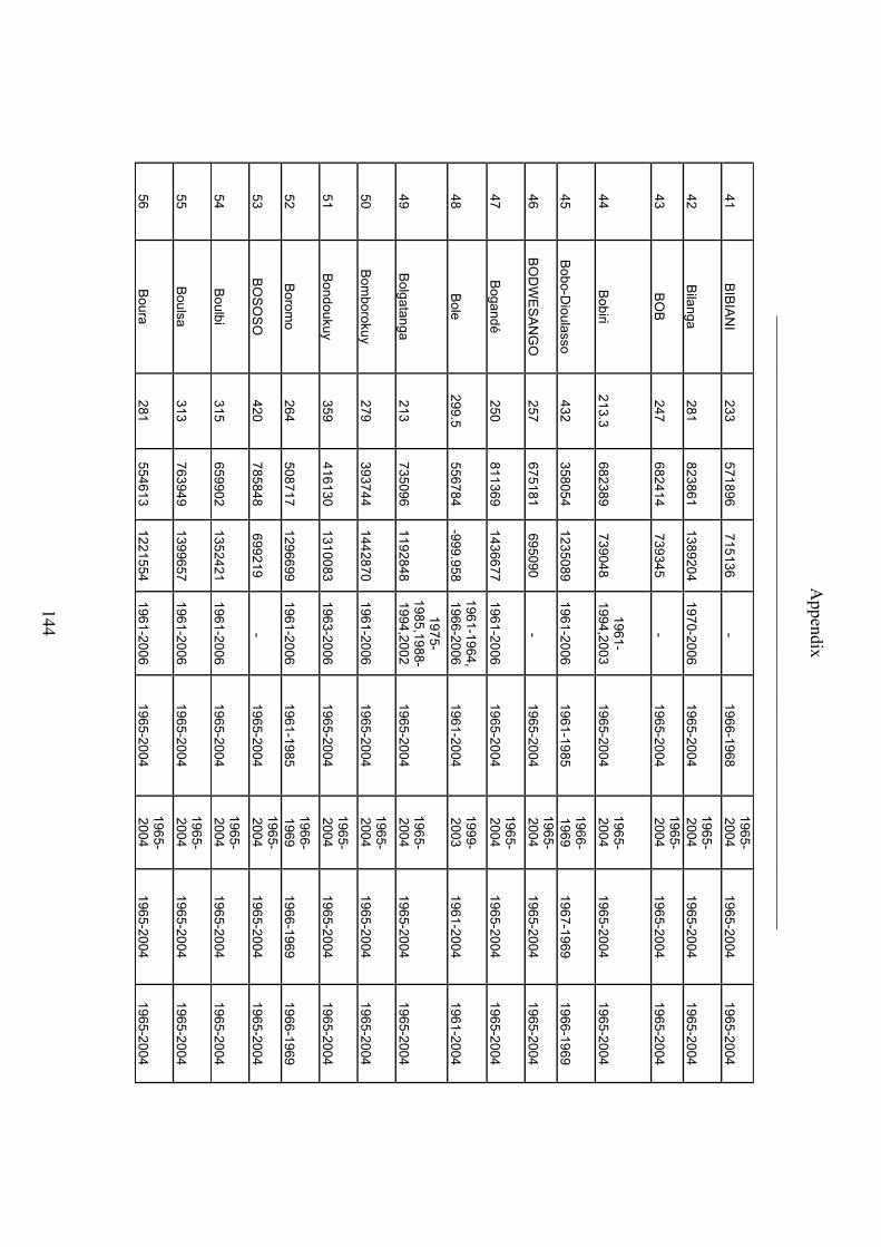
Appendix
_____________________________________________________________________
144
41
BIB
IAN
I 233
571
896
715
136
-
1966-19
68
1965-
2004
196
5-2004
196
5-2004
42
Bila
nga
281
82386
1
13892
04
1970-20
06
1965-20
04
1965-
2004
196
5-2004
196
5-2004
43
BO
B
247
68241
4
73934
5
- 196
5-2004
196
5-200
4
1965-20
04
1965-20
04
44
Bobiri
213.3
68238
9
73904
8
1961-
1994,20
03
1965-20
04
1965-
2004
196
5-2004
196
5-2004
45
Bobo-D
ioulasso
432
35805
4
12350
89
1961-20
06
1961-19
85
1966-
1969
196
7-1969
196
6-1969
46 B
OD
WE
SA
NG
O
257 675181
695090 -
1965-2004 196
5-200
4
1965-20
04
1965-20
04
47
Boga
ndé
250
811
369
143
6677
196
1-2006
196
5-2004
196
5-200
4
1965-20
04
1965-20
04
48
Bole
299.5
556
784
-999.9
58
1961-19
64, 196
6-2006
196
1-2004
199
9-200
3
1961-20
04
1961-20
04
49
Bolg
atanga
213
735
096
119
2848
1975-
1985,19
88-199
4,2002
196
5-2004
196
5-200
4
1965-20
04
1965-20
04
50
Bom
borokuy
279
39374
4
14428
70
1961-20
06
1965-20
04
1965-
2004
196
5-2004
196
5-2004
51
Bond
oukuy
359
41613
0
13100
83
1963-20
06
1965-20
04
1965-
2004
196
5-2004
196
5-2004
52
Borom
o
264
50871
7
12966
99
1961-20
06
1961-19
85
1966-
1969
196
6-1969
196
6-1969
53
BO
SO
SO
420
785
848
699
219
-
1965-20
04
1965-
2004
196
5-2004
196
5-2004
54
Boulbi
315
65990
2
13524
21
1961-20
06
1965-20
04
1965-
2004
196
5-2004
196
5-2004
55
Boulsa
313
763
949
139
9657
196
1-2006
196
5-2004
196
5-200
4
1965-20
04
1965-20
04
56
Boura
281
554
613
122
1554
196
1-2006
196
5-2004
196
5-200
4
1965-20
04
1965-20
04
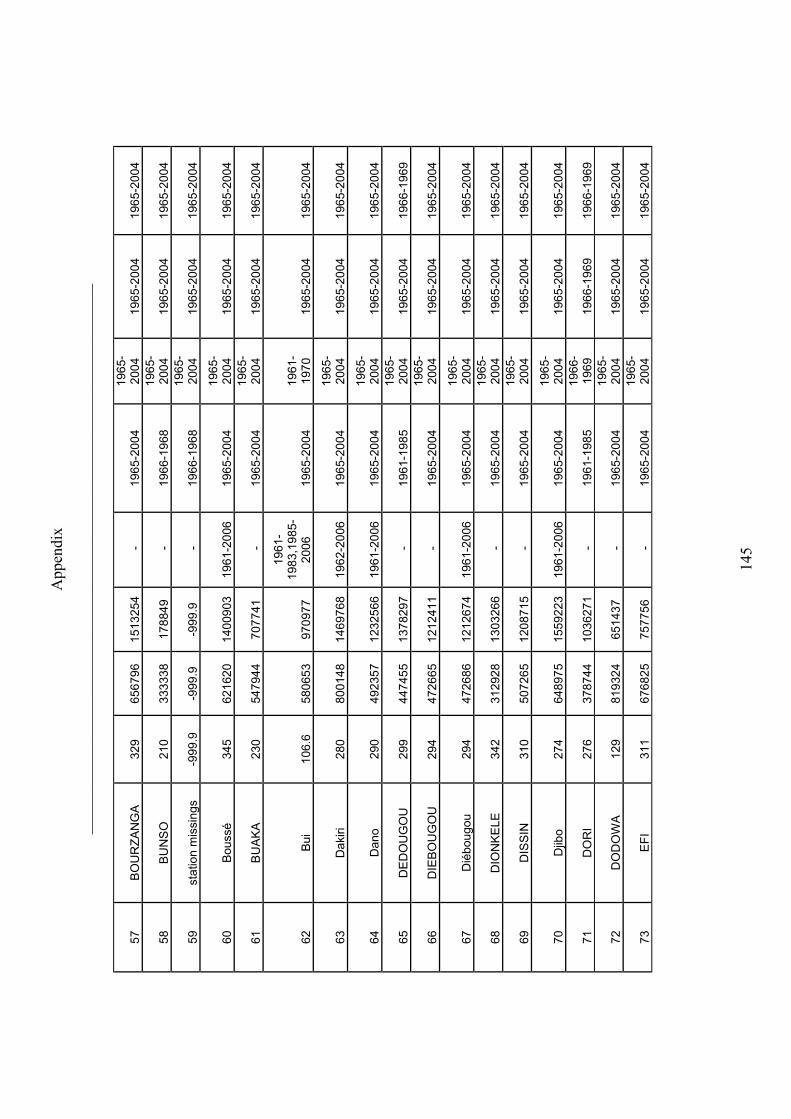
App
endi
x
____
____
____
____
____
____
____
____
____
____
____
____
____
____
____
____
____
_
145
57
BO
UR
ZA
NG
A
329
65
679
6
151
3254
-
19
65-
2004
19
65-
200
4
196
5-20
04
196
5-20
04
58
BU
NS
O
210
33
333
8
178
849
-
19
66-
1968
19
65-
200
4
196
5-20
04
196
5-20
04
59
stat
ion
mis
sing
s -9
99.9
-9
99.9
-9
99.9
-
19
66-
1968
19
65-
200
4
196
5-20
04
196
5-20
04
60
Bou
ssé
34
5
621
620
14
009
03
196
1-20
06
196
5-20
04
196
5-20
04
19
65-
2004
19
65-
2004
61
BU
AK
A
230
54
794
4
707
741
-
19
65-
2004
19
65-
200
4
196
5-20
04
196
5-20
04
62
Bui
10
6.6
58
065
3
970
977
196
1-19
83,
1985
-20
06
19
65-
2004
19
61-
197
0
196
5-20
04
196
5-20
04
63
Dak
iri
280
80
014
8
146
9768
19
62-
2006
19
65-
2004
19
65-
200
4
196
5-20
04
196
5-20
04
64
Dan
o
290
49
235
7
123
2566
19
61-
2006
19
65-
2004
19
65-
200
4
196
5-20
04
196
5-20
04
65
DE
DO
UG
OU
29
9
447
455
13
782
97
-
196
1-19
85
196
5-20
04
19
65-
2004
19
66-
1969
66
DIE
BO
UG
OU
29
4
472
665
12
124
11
-
196
5-20
04
196
5-20
04
19
65-
2004
19
65-
2004
67
Dié
bou
gou
29
4
472
686
12
126
74
196
1-20
06
196
5-20
04
196
5-20
04
19
65-
2004
19
65-
2004
68
DIO
NK
ELE
34
2
312
928
13
032
66
-
196
5-20
04
196
5-20
04
19
65-
2004
19
65-
2004
69
DIS
SIN
31
0
507
265
12
087
15
-
196
5-20
04
196
5-20
04
19
65-
2004
19
65-
2004
70
Djib
o
274
64
897
5
155
9223
19
61-
2006
19
65-
2004
19
65-
200
4
196
5-20
04
196
5-20
04
71
DO
RI
276
37
874
4
103
6271
-
19
61-
1985
19
66-
196
9
196
6-19
69
196
6-19
69
72
DO
DO
WA
12
9
819
324
65
143
7
-
196
5-20
04
196
5-20
04
19
65-
2004
19
65-
2004
73
EF
I 31
1
676
825
75
775
6
-
196
5-20
04
196
5-20
04
19
65-
2004
19
65-
2004
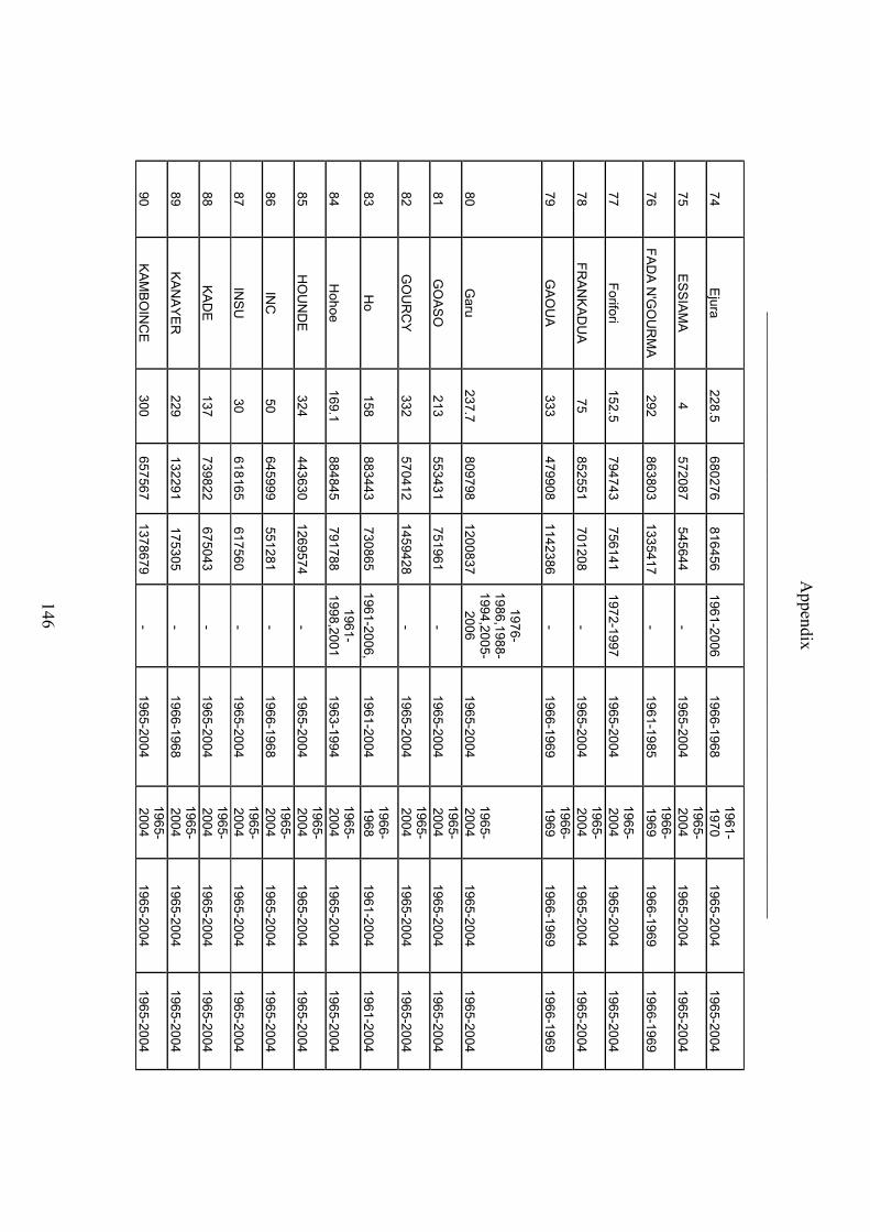
Appendix
_____________________________________________________________________
146
74
Ejura
228.5
680
276
816
456
196
1-2006
196
6-1968
196
1-197
0
1965-20
04
1965-20
04
75 E
SS
IAM
A
4 572087
545644
- 1965-2004
1965-
2004
196
5-2004
196
5-2004
76
FA
DA
N'G
OU
RM
A
292
86380
3
13354
17
- 196
1-1985
196
6-196
9
1966-19
69
1966-19
69
77
Forifori
152.5
79474
3
75614
1
1972-19
97
1965-20
04
1965-
2004
196
5-2004
196
5-2004
78
FR
AN
KA
DU
A
75
85255
1
70120
8
- 196
5-2004
196
5-200
4
1965-20
04
1965-20
04
79
GA
OU
A
333
47990
8
11423
86
- 196
6-1969
196
6-196
9
1966-19
69
1966-19
69
80
Garu
237.7
80979
8
12008
37
1976-
1986,19
88-199
4,2005-
2006
196
5-2004
196
5-200
4
1965-20
04
1965-20
04
81
GO
AS
O
213
55343
1
75196
1
- 196
5-2004
196
5-200
4
1965-20
04
1965-20
04
82
GO
UR
CY
332
570
412
145
9428
-
1965-20
04
1965-
2004
196
5-2004
196
5-2004
83
Ho
158
883
443
730
865
196
1-2006,
1961-20
04
1966-
1968
196
1-2004
196
1-2004
84
Hoh
oe
169.1
88484
5
79178
8
1961-
1998,20
01
1963-19
94
1965-
2004
196
5-2004
196
5-2004
85
HO
UN
DE
324
443
630
126
9574
-
1965-20
04
1965-
2004
196
5-2004
196
5-2004
86
INC
50
645
999
551
281
-
1966-19
68
1965-
2004
196
5-2004
196
5-2004
87
INS
U
30
61816
5
61756
0
- 196
5-2004
196
5-200
4
1965-20
04
1965-20
04
88
KA
DE
137
739
822
675
043
-
1965-20
04
1965-
2004
196
5-2004
196
5-2004
89 K
AN
AY
ER
229
132291 175
305 -
1966-1968 196
5-200
4
1965-20
04
1965-20
04
90
KA
MB
OIN
CE
300
657
567
137
8679
-
1965-20
04
1965-
2004
196
5-2004
196
5-2004
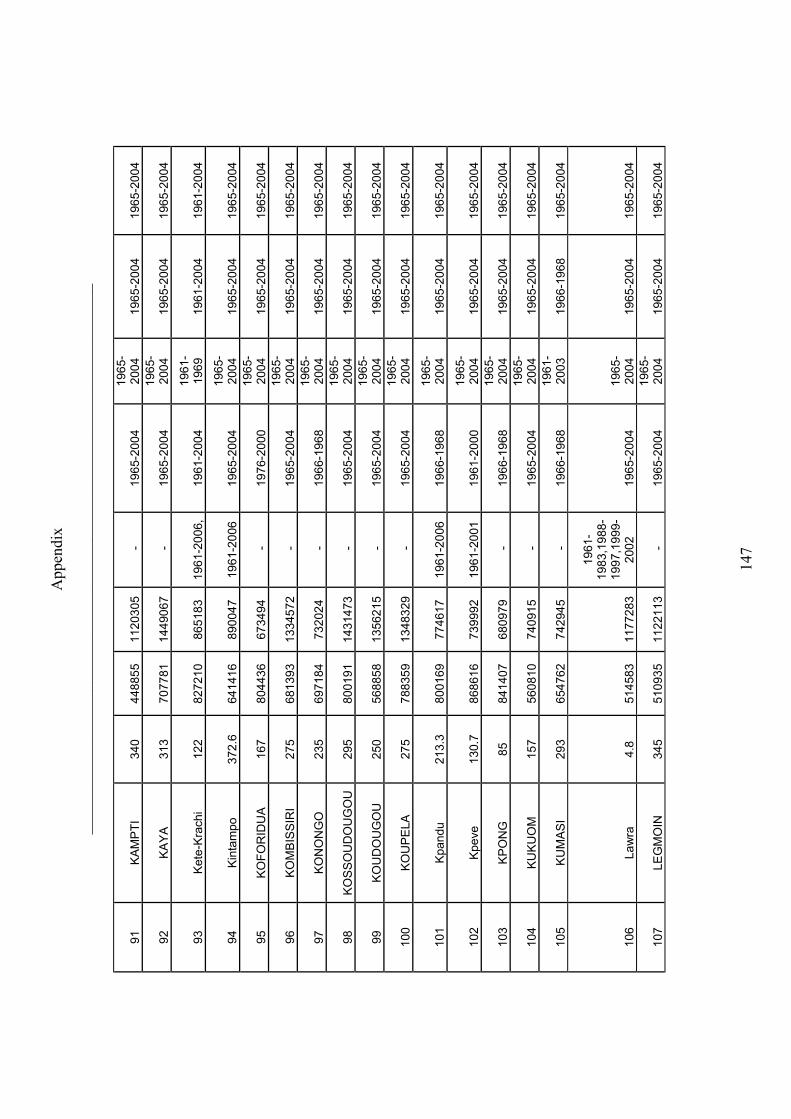
App
endi
x
____
____
____
____
____
____
____
____
____
____
____
____
____
____
____
____
____
_
147
91
KA
MP
TI
340
44
885
5
112
0305
-
19
65-
2004
19
65-
200
4
196
5-20
04
196
5-20
04
92
KA
YA
31
3 70
7781
14
490
67
-
1965
-200
4 19
65-
200
4
196
5-20
04
196
5-20
04
93
Ket
e-K
rach
i 12
2
827
210
86
518
3
196
1-20
06,
196
1-20
04
196
1-19
69
19
61-
2004
19
61-
2004
94
Kin
tam
po
37
2.6
64
141
6
890
047
19
61-
2006
19
65-
2004
19
65-
200
4
196
5-20
04
196
5-20
04
95
KO
FO
RID
UA
16
7
804
436
67
349
4
-
197
6-20
00
196
5-20
04
19
65-
2004
19
65-
2004
96
KO
MB
ISS
IRI
275
68
139
3
133
4572
-
19
65-
2004
19
65-
200
4
196
5-20
04
196
5-20
04
97
KO
NO
NG
O
235
69
718
4
732
024
-
19
66-
1968
19
65-
200
4
196
5-20
04
196
5-20
04
98
KO
SS
OU
DO
UG
OU
29
5
800
191
14
314
73
-
196
5-20
04
196
5-20
04
19
65-
2004
19
65-
2004
99
KO
UD
OU
GO
U
250
56
885
8
135
6215
-
19
65-
2004
19
65-
200
4
196
5-20
04
196
5-20
04
100
K
OU
PE
LA
275
78
835
9
134
8329
-
19
65-
2004
19
65-
200
4
196
5-20
04
196
5-20
04
101
K
pan
du
213.
3
800
169
77
461
7
196
1-20
06
196
6-19
68
196
5-20
04
19
65-
2004
19
65-
2004
102
K
peve
13
0.7
86
861
6
739
992
19
61-
2001
19
61-
2000
19
65-
200
4
196
5-20
04
196
5-20
04
103
K
PO
NG
85
84
140
7
680
979
-
19
66-
1968
19
65-
200
4
196
5-20
04
196
5-20
04
104
K
UK
UO
M
157
56
081
0
740
915
-
19
65-
2004
19
65-
200
4
196
5-20
04
196
5-20
04
105
K
UM
AS
I 29
3
654
762
74
294
5
-
196
6-19
68
196
1-20
03
19
66-
1968
19
65-
2004
106
La
wra
4.
8
514
583
11
772
83
196
1-19
83,
1988
-19
97,
1999
-20
02
19
65-
2004
19
65-
200
4
196
5-20
04
196
5-20
04
107
LE
GM
OIN
34
5
510
935
11
221
13
-
196
5-20
04
196
5-20
04
19
65-
2004
19
65-
2004
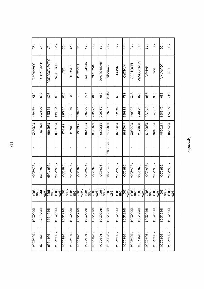
Appendix
_____________________________________________________________________
148
108
LEO
347
598
271
122
7290
-
1965-20
04
1965-
2004
196
5-2004
196
5-2004
109
LOU
MA
NA
320
242
831
117
0988
-
1965-20
04
1965-
2004
196
5-2004
196
5-2004
110
MA
N
226
79871
5
12194
36
- 196
5-2004
196
5-200
4
1965-20
04
1965-20
04
111
MA
NG
A
286
71073
6
12905
13
- 196
5-2004
196
5-200
4
1965-20
04
1965-20
04
112
MA
NG
OD
AR
A
260
35196
6
10947
73
- 196
5-2004
196
5-200
4
1965-20
04
1965-20
04
113
MO
GT
ED
O
272
73564
7
13589
62
- 196
5-2004
196
5-200
4
1965-20
04
1965-20
04
114
NA
NO
RO
312
588
655
140
2345
-
1965-20
04
1965-
2004
196
5-2004
196
5-2004
115 N
AS
SO
339
343486 123
8578 -
1965-2004 196
5-200
4
1965-20
04
1965-20
04
116
Navro
ngo
201.3
70766
9
12055
74
1961-20
06,196
1-2004
198
7-200
3
1966-20
04
1961-20
04
117
NIA
NG
OLO
KO
320
290
055
113
5635
-
1965-20
04
1965-
2004
196
5-2004
196
5-2004
118
NIA
OG
HO
240
743
366
130
1818
-
1965-20
04
1965-
2004
196
5-2004
196
5-2004
119
NO
MO
UN
OU
274
358
393
131
2238
-
1965-20
04
1965-
2004
196
5-2004
196
5-2004
120
NS
AW
AM
47
793
500
643
932
-
1965-20
04
1965-
2004
196
5-2004
196
5-2004
121
NU
NG
UA
50
823
188
618
254
-
1965-20
04
1965-
2004
196
5-2004
196
5-2004
122
OD
A
200
72328
8
65470
2
- 196
5-2004
196
5-200
4
1965-20
04
1965-20
04
123
OR
OD
AR
A
523
29054
4
12149
10
- 196
5-2004
196
5-200
4
1965-20
04
1965-20
04
124
OU
AG
AD
OU
GO
U
303
66126
2
13657
95
- 196
6-1969
196
6-196
9
1966-19
69
1966-19
69
125 O
UA
HIG
OU
YA
329
561285 150
1797 -
1966-1969 196
6-196
9
1966-19
69
1966-19
69
126
OU
AR
KO
YE
315
427
427
133
5952
-
1965-20
04
1965-
2004
196
5-2004
196
5-2004
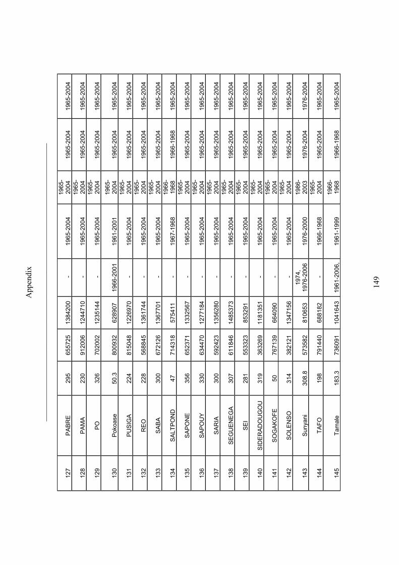
App
endi
x
____
____
____
____
____
____
____
____
____
____
____
____
____
____
____
____
____
_
149
127
PA
BR
E
295
6557
25
1384
200
-
19
65-2
004
196
5-20
04
19
65-
2004
19
65-
2004
128
P
AM
A
230
91
200
6
124
4710
-
19
65-
2004
19
65-
200
4
196
5-20
04
196
5-20
04
129
P
O
326
70
200
2
123
5144
-
19
65-
2004
19
65-
200
4
196
5-20
04
196
5-20
04
130
P
okoa
se
50.3
80
093
2
628
907
19
66-
2001
19
61-
2001
19
65-
200
4
196
5-20
04
196
5-20
04
131
P
US
IGA
22
4
815
048
12
269
70
-
196
5-20
04
196
5-20
04
19
65-
2004
19
65-
2004
132
R
EO
22
8
568
845
13
617
44
-
196
5-20
04
196
5-20
04
19
65-
2004
19
65-
2004
133
SA
BA
30
0 67
2126
13
677
01
-
1965
-200
4 19
65-
200
4
196
5-20
04
196
5-20
04
134
S
ALT
PO
ND
47
71
431
8
575
411
-
19
67-
1968
19
66-
196
8
196
6-19
68
196
5-20
04
135
SA
PO
NE
35
6 65
2371
13
325
67
-
1965
-200
4 19
65-
200
4
196
5-20
04
196
5-20
04
136
SA
PO
UY
33
0 63
4470
12
771
84
-
1965
-200
4 19
65-
200
4
196
5-20
04
196
5-20
04
137
S
AR
IA
300
59
242
3
135
6280
-
19
65-
2004
19
65-
200
4
196
5-20
04
196
5-20
04
138
S
EG
UE
NE
GA
30
7
611
846
14
853
73
-
196
5-20
04
196
5-20
04
19
65-
2004
19
65-
2004
139
S
EI
281
55
332
3
853
291
-
19
65-
2004
19
65-
200
4
196
5-20
04
196
5-20
04
140
S
IDE
RA
DO
UG
OU
31
9
363
269
11
813
51
-
196
5-20
04
196
5-20
04
19
65-
2004
19
65-
2004
141
S
OG
AK
OF
E
50
767
139
66
409
0
-
196
5-20
04
196
5-20
04
19
65-
2004
19
65-
2004
142
S
OLE
NS
O
314
38
212
1
134
7156
-
19
65-
2004
19
65-
200
4
196
5-20
04
196
5-20
04
143
S
unya
ni
308.
8
573
582
81
065
3
197
4,
197
6-20
06
197
6-20
00
198
6-20
03
19
76-
2004
19
76-
2004
144
T
AF
O
198
79
144
0
688
182
-
19
66-
1968
19
65-
200
4
196
5-20
04
196
5-20
04
145
T
amal
e 18
3.3
73
609
1
104
1643
19
61-
2006
,19
61-
1999
19
66-
196
8
196
6-19
68
196
5-20
04
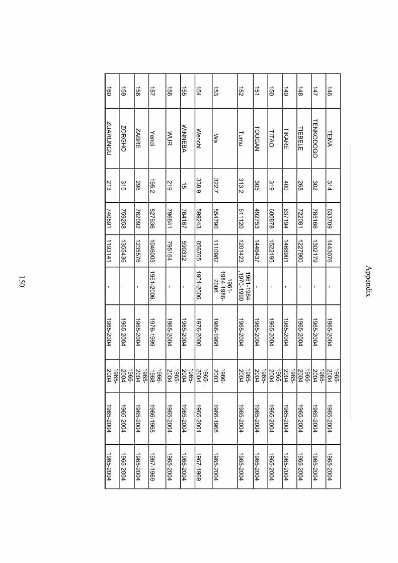
Appendix
_____________________________________________________________________
150
146
TE
MA
314
633
709
144
3076
-
1965-20
04
1965-
2004
196
5-2004
196
5-2004
147
TE
NK
OD
OG
O
302
78516
6
13021
79
- 196
5-2004
196
5-200
4
1965-20
04
1965-20
04
148 T
IEB
ELE
268
722081 122
7900 -
1965-2004 196
5-200
4
1965-20
04
1965-20
04
149
TIK
AR
E
400
63719
4
14689
01
- 196
5-2004
196
5-200
4
1965-20
04
1965-20
04
150
TIT
AO
319
600
878
152
2195
-
1965-20
04
1965-
2004
196
5-2004
196
5-2004
151
TO
UG
AN
305
492
753
144
6437
-
1965-20
04
1965-
2004
196
5-2004
196
5-2004
152
Tum
u 313.2
611
120
120
1423
196
1-1964
,1970-1990
1965-20
04
1965-
2004
196
5-2004
196
5-2004
153
Wa
322.7
55479
0
11109
82
1961-
1984,19
86-200
6
1966-19
68
1986-
2003
196
6-1968
196
5-2004
154
Wenchi
338.9
59924
3
85676
5
1961-20
06,197
6-2000
196
5-200
4
1965-20
04
1967-19
69
155 W
INN
EB
A
15 764167
590332
- 1965-2004
1965-
2004
196
5-2004
196
5-2004
156
WU
R
219
79684
1
79516
4
- 196
5-2004
196
5-200
4
1965-20
04
1965-20
04
157
Yend
i 195.2
827
636
104
6005
196
1-2006,
1976-19
99
1966-
1968
196
6-1968
196
7-1969
158
ZA
BR
E
296
76209
2
12355
76
- 196
5-2004
196
5-200
4
1965-20
04
1965-20
04
159
ZO
RG
HO
315
759
258
135
5436
-
1965-20
04
1965-
2004
196
5-2004
196
5-2004
160
ZU
AR
UN
GU
213
740
591
119
3141
-
1965-20
04
1965-
2004
196
5-2004
196
5-2004
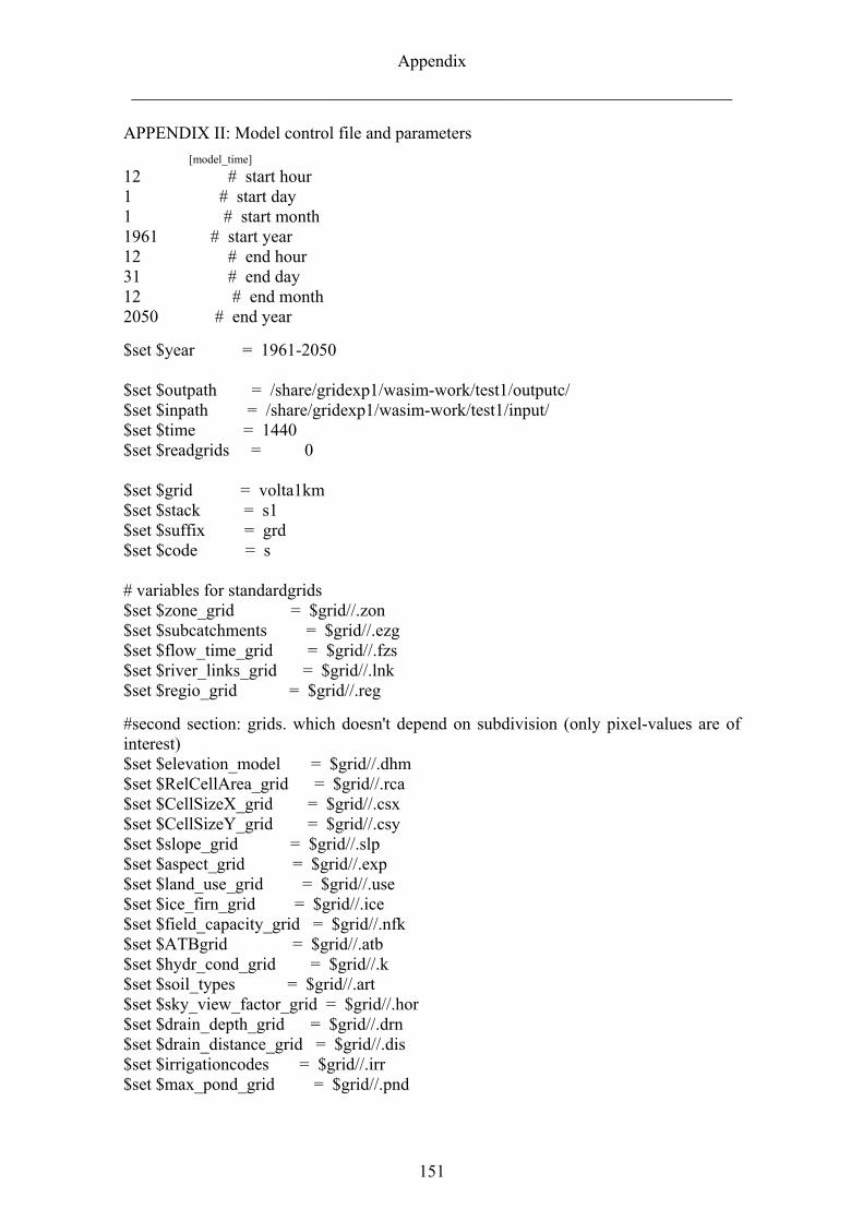
Appendix
_____________________________________________________________________
151
APPENDIX II: Model control file and parameters
[model_time]
12 # start hour 1 # start day 1 # start month 1961 # start year 12 # end hour 31 # end day 12 # end month 2050 # end year
$set $year = 1961-2050 $set $outpath = /share/gridexp1/wasim-work/test1/outputc/ $set $inpath = /share/gridexp1/wasim-work/test1/input/ $set $time = 1440 $set $readgrids = 0 $set $grid = volta1km $set $stack = s1 $set $suffix = grd $set $code = s # variables for standardgrids $set $zone_grid = $grid//.zon $set $subcatchments = $grid//.ezg $set $flow_time_grid = $grid//.fzs $set $river_links_grid = $grid//.lnk $set $regio_grid = $grid//.reg
#second section: grids. which doesn't depend on subdivision (only pixel-values are of interest) $set $elevation_model = $grid//.dhm $set $RelCellArea_grid = $grid//.rca $set $CellSizeX_grid = $grid//.csx $set $CellSizeY_grid = $grid//.csy $set $slope_grid = $grid//.slp $set $aspect_grid = $grid//.exp $set $land_use_grid = $grid//.use $set $ice_firn_grid = $grid//.ice $set $field_capacity_grid = $grid//.nfk $set $ATBgrid = $grid//.atb $set $hydr_cond_grid = $grid//.k $set $soil_types = $grid//.art $set $sky_view_factor_grid = $grid//.hor $set $drain_depth_grid = $grid//.drn $set $drain_distance_grid = $grid//.dis $set $irrigationcodes = $grid//.irr $set $max_pond_grid = $grid//.pnd
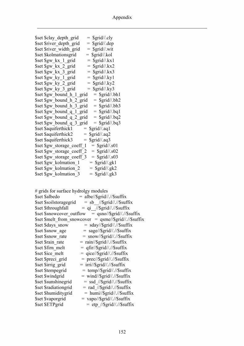
Appendix
_____________________________________________________________________
152
$set $clay_depth_grid = $grid//.cly $set $river_depth_grid = $grid//.dep $set $river_width_grid = $grid//.wit $set $kolmationsgrid = $grid//.kol $set $gw_kx_1_grid = $grid//.kx1 $set $gw_kx_2_grid = $grid//.kx2 $set $gw_kx_3_grid = $grid//.kx3 $set $gw_ky_1_grid = $grid//.ky1 $set $gw_ky_2_grid = $grid//.ky2 $set $gw_ky_3_grid = $grid//.ky3 $set $gw_bound_h_1_grid = $grid//.bh1 $set $gw_bound_h_2_grid = $grid//.bh2 $set $gw_bound_h_3_grid = $grid//.bh3 $set $gw_bound_q_1_grid = $grid//.bq1 $set $gw_bound_q_2_grid = $grid//.bq2 $set $gw_bound_q_3_grid = $grid//.bq3 $set $aquiferthick1 = $grid//.aq1 $set $aquiferthick2 = $grid//.aq2 $set $aquiferthick3 = $grid//.aq3 $set $gw_storage_coeff_1 = $grid//.s01 $set $gw_storage_coeff_2 = $grid//.s02 $set $gw_storage_coeff_3 = $grid//.s03 $set $gw_kolmation_1 = $grid//.gk1 $set $gw_kolmation_2 = $grid//.gk2 $set $gw_kolmation_3 = $grid//.gk3 # grids for surface hydrolgy modules $set $albedo = albe//$grid//.//$suffix $set $soilstoragegrid = sb__//$grid//.//$suffix $set $throughfall = qi__//$grid//.//$suffix $set $snowcover_outflow = qsno//$grid//.//$suffix $set $melt_from_snowcover = qsme//$grid//.//$suffix $set $days_snow = sday//$grid//.//$suffix $set $snow_age = sage//$grid//.//$suffix $set $snow_rate = snow//$grid//.//$suffix $set $rain_rate = rain//$grid//.//$suffix $set $firn_melt = qfir//$grid//.//$suffix $set $ice_melt = qice//$grid//.//$suffix $set $preci_grid = prec//$grid//.//$suffix $set $irrig_grid = irri//$grid//.//$suffix $set $tempegrid = temp//$grid//.//$suffix $set $windgrid = wind//$grid//.//$suffix $set $sunshinegrid = ssd_//$grid//.//$suffix $set $radiationgrid = rad_//$grid//.//$suffix $set $humiditygrid = humi//$grid//.//$suffix $set $vaporgrid = vapo//$grid//.//$suffix $set $ETPgrid = etp_//$grid//.//$suffix
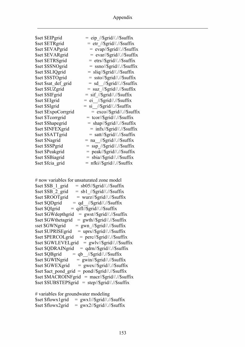
Appendix
_____________________________________________________________________
153
$set $EIPgrid = eip_//$grid//.//$suffix $set $ETRgrid = etr_//$grid//.//$suffix $set $EVAPgrid = evap//$grid//.//$suffix $set $EVARgrid = evar//$grid//.//$suffix $set $ETRSgrid = etrs//$grid//.//$suffix $set $SSNOgrid = ssno//$grid//.//$suffix $set $SLIQgrid = sliq//$grid//.//$suffix $set $SSTOgrid = ssto//$grid//.//$suffix $set $sat_def_grid = sd__//$grid//.//$suffix $set $SUZgrid = suz_//$grid//.//$suffix $set $SIFgrid = sif_//$grid//.//$suffix $set $EIgrid = ei__//$grid//.//$suffix $set $SIgrid = si__//$grid//.//$suffix $set $ExpoCorrgrid = exco//$grid//.//$suffix $set $Tcorrgrid = tcor//$grid//.//$suffix $set $Shapegrid = shap//$grid//.//$suffix $set $INFEXgrid = infx//$grid//.//$suffix $set $SATTgrid = satt//$grid//.//$suffix $set $Nagrid = na__//$grid//.//$suffix $set $SSPgrid = ssp_//$grid//.//$suffix $set $Peakgrid = peak//$grid//.//$suffix $set $SBiagrid = sbia//$grid//.//$suffix $set $fcia_grid = nfki//$grid//.//$suffix # now variables for unsaturated zone model $set $SB_1_grid = sb05//$grid//.//$suffix $set $SB_2_grid = sb1_//$grid//.//$suffix $set $ROOTgrid = wurz//$grid//.//$suffix $set $QDgrid = qd__//$grid//.//$suffix $set $QIgrid = qifl//$grid//.//$suffix $set $GWdepthgrid = gwst//$grid//.//$suffix $set $GWthetagrid = gwth//$grid//.//$suffix $set $GWNgrid = gwn_//$grid//.//$suffix $set $UPRISEgrid = uprs//$grid//.//$suffix $set $PERCOLgrid = perc//$grid//.//$suffix $set $GWLEVELgrid = gwlv//$grid//.//$suffix $set $QDRAINgrid = qdrn//$grid//.//$suffix $set $QBgrid = qb__//$grid//.//$suffix $set $GWINgrid = gwin//$grid//.//$suffix $set $GWEXgrid = gwex//$grid//.//$suffix $set $act_pond_grid = pond//$grid//.//$suffix $set $MACROINFgrid = macr//$grid//.//$suffix $set $SUBSTEPSgrid = step//$grid//.//$suffix # variables for groundwater modeling $set $flowx1grid = gwx1//$grid//.//$suffix $set $flowx2grid = gwx2//$grid//.//$suffix
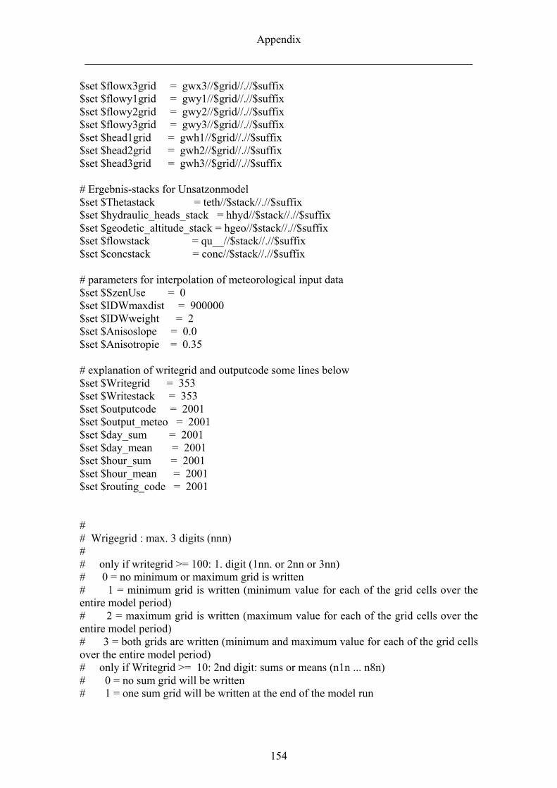
Appendix
_____________________________________________________________________
154
$set $flowx3grid = gwx3//$grid//.//$suffix $set $flowy1grid = gwy1//$grid//.//$suffix $set $flowy2grid = gwy2//$grid//.//$suffix $set $flowy3grid = gwy3//$grid//.//$suffix $set $head1grid = gwh1//$grid//.//$suffix $set $head2grid = gwh2//$grid//.//$suffix $set $head3grid = gwh3//$grid//.//$suffix # Ergebnis-stacks for Unsatzonmodel $set $Thetastack = teth//$stack//.//$suffix $set $hydraulic_heads_stack = hhyd//$stack//.//$suffix $set $geodetic_altitude_stack = hgeo//$stack//.//$suffix $set $flowstack = qu__//$stack//.//$suffix $set $concstack = conc//$stack//.//$suffix # parameters for interpolation of meteorological input data $set $SzenUse = 0 $set $IDWmaxdist = 900000 $set $IDWweight = 2 $set $Anisoslope = 0.0 $set $Anisotropie = 0.35 # explanation of writegrid and outputcode some lines below $set $Writegrid = 353 $set $Writestack = 353 $set $outputcode = 2001 $set $output_meteo = 2001 $set $day_sum = 2001 $set $day_mean = 2001 $set $hour_sum = 2001 $set $hour_mean = 2001 $set $routing_code = 2001 # # Wrigegrid : max. 3 digits (nnn) # # only if writegrid >= 100: 1. digit (1nn. or 2nn or 3nn) # 0 = no minimum or maximum grid is written # 1 = minimum grid is written (minimum value for each of the grid cells over the entire model period) # 2 = maximum grid is written (maximum value for each of the grid cells over the entire model period) # 3 = both grids are written (minimum and maximum value for each of the grid cells over the entire model period) # only if Writegrid >= 10: 2nd digit: sums or means (n1n ... n8n) # 0 = no sum grid will be written # 1 = one sum grid will be written at the end of the model run

Appendix
_____________________________________________________________________
155
# 2 = one sum grid per model year # 3 = one sum grid per model month # 4 = one sum grid per day (only. if timestep < 1 day) # 5 = one mean value grid at the end of the model run # 6 = one mean value grid per model year # 7 = one mean value grid per month # 8 = one mean value grid per day # last digit (nn1 .. nn5) (for actual values. not for Sums or means) # 1 = (over)write each timestep into the same grid (for security in case of model crashs) # 2 = write grids each timestep to new files. the name is build from the first 4 letters # of the regular grid name and then from the number of month. day and hour (hoer as file extension) # example: tempm500.grd will become prec0114.07 for 14.January. 7:00 # 3 = only the last grid of the model run will be stored # 4 = the grid from the last hour of each day (24:00) will be stored (for each day the same file will be overwritten) # 5 = like 4. but each day a new grid file is created (like for code 2) # # outputcode (for statistic files for zones or subcatchments) # # the Codes behind the names of the statistic files have the meaning of: # <1000 : no output # 1<nnn> : spatial mean values for the entire basin. averaged in time over <nnn> intervals (timesteps) # 2<nnn> : spatial mean values for all zones (subbasin) and for the entire basin. averaged in time over <nnn> intervals (timesteps) # 3<nnn> : spatial means for the entire basin. added up in time over <nnn> intervals (timesteps) # 4<nnn> : spatial means for all zones (subbasin) and for the entire basin. added up in time over <nnn> intervals (timesteps) # 5<nnn> : spatial means for the entire basin and for those subbasins which are spcified in the output-list. averaged in time over <nnn> intervals # 6<nnn> : spatial means for the entire basin and for those subbasins which are spcified in the output-list. added up in time over <nnn> intervals # # example: # 2001 = per timestep for all subcatchments (and for the entire basin) one (spatially averaged) value. # 2004 = each 4 time steps one averaged value over the last 4 time steps for all subcatchments and for the entire basin. # 4024 = Sums of the mean subcatchment/entire basin values of the timesteps over 24 timesteps (e.g. daily rain sums for subcatchments). # 3120 = averaged values (over 120 time steps!) only for the entire basin (spatially averaged) # 5012 = averaged values (over 12 timesteps) as spatial averages for the entire basin and for each of the subbasins specified in the output-list
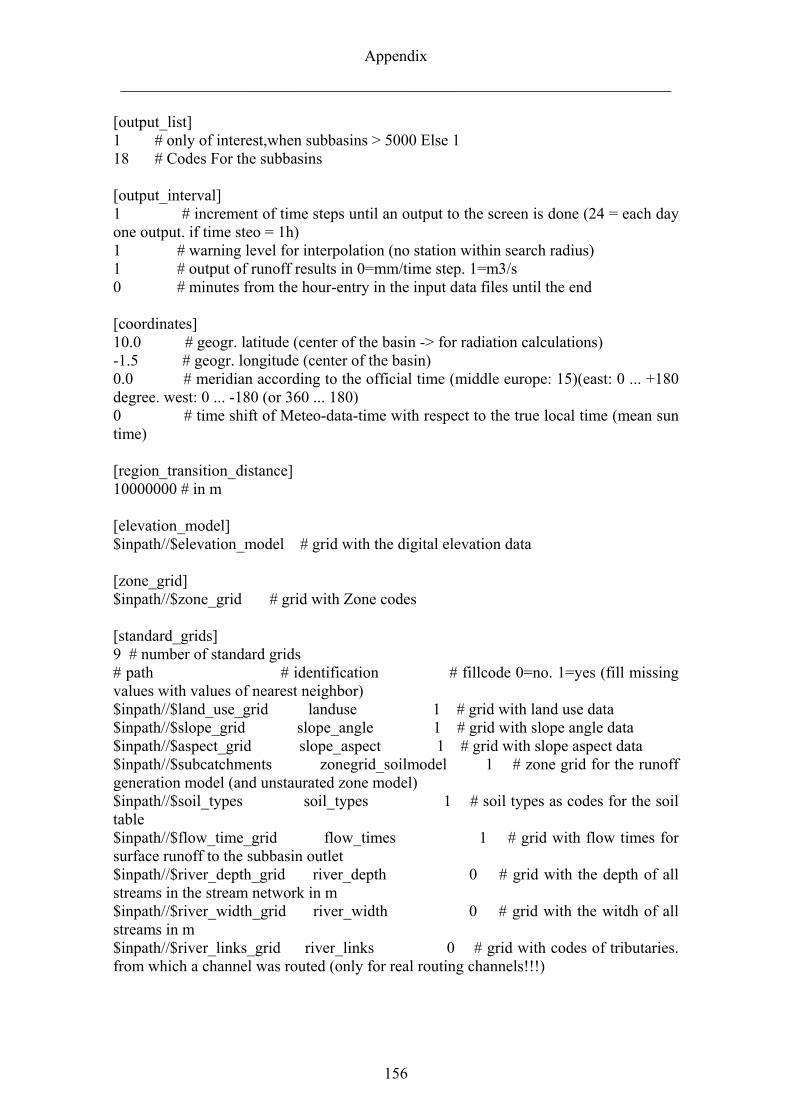
Appendix
_____________________________________________________________________
156
[output_list] 1 # only of interest,when subbasins > 5000 Else 1 18 # Codes For the subbasins [output_interval] 1 # increment of time steps until an output to the screen is done (24 = each day one output. if time steo = 1h) 1 # warning level for interpolation (no station within search radius) 1 # output of runoff results in 0=mm/time step. 1=m3/s 0 # minutes from the hour-entry in the input data files until the end [coordinates] 10.0 # geogr. latitude (center of the basin -> for radiation calculations) -1.5 # geogr. longitude (center of the basin) 0.0 # meridian according to the official time (middle europe: 15)(east: 0 ... +180 degree. west: 0 ... -180 (or 360 ... 180) 0 # time shift of Meteo-data-time with respect to the true local time (mean sun time) [region_transition_distance] 10000000 # in m [elevation_model] $inpath//$elevation_model # grid with the digital elevation data [zone_grid] $inpath//$zone_grid # grid with Zone codes [standard_grids] 9 # number of standard grids # path # identification # fillcode 0=no. 1=yes (fill missing values with values of nearest neighbor) $inpath//$land_use_grid landuse 1 # grid with land use data $inpath//$slope_grid slope_angle 1 # grid with slope angle data $inpath//$aspect_grid slope_aspect 1 # grid with slope aspect data $inpath//$subcatchments zonegrid_soilmodel 1 # zone grid for the runoff generation model (and unstaurated zone model) $inpath//$soil_types soil_types 1 # soil types as codes for the soil table $inpath//$flow_time_grid flow_times 1 # grid with flow times for surface runoff to the subbasin outlet $inpath//$river_depth_grid river_depth 0 # grid with the depth of all streams in the stream network in m $inpath//$river_width_grid river_width 0 # grid with the witdh of all streams in m $inpath//$river_links_grid river_links 0 # grid with codes of tributaries. from which a channel was routed (only for real routing channels!!!)
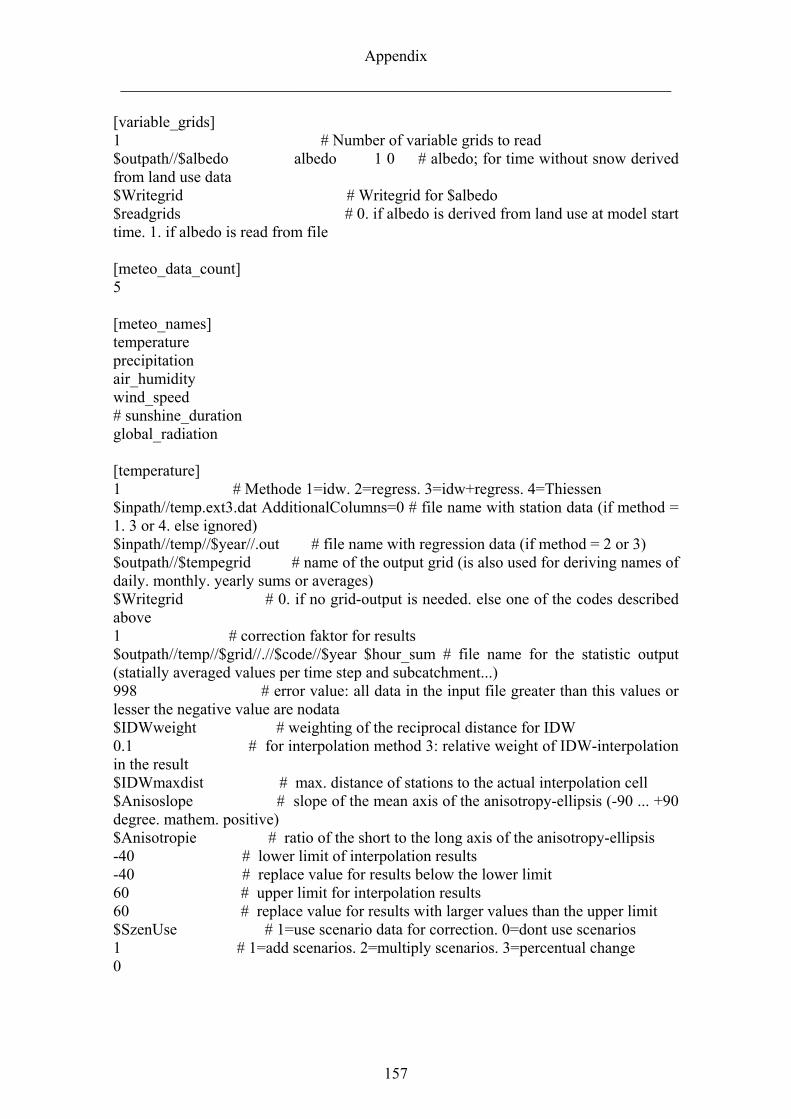
Appendix
_____________________________________________________________________
157
[variable_grids] 1 # Number of variable grids to read $outpath//$albedo albedo 1 0 # albedo; for time without snow derived from land use data $Writegrid # Writegrid for $albedo $readgrids # 0. if albedo is derived from land use at model start time. 1. if albedo is read from file [meteo_data_count] 5 [meteo_names] temperature precipitation air_humidity wind_speed # sunshine_duration global_radiation [temperature] 1 # Methode 1=idw. 2=regress. 3=idw+regress. 4=Thiessen $inpath//temp.ext3.dat AdditionalColumns=0 # file name with station data (if method = 1. 3 or 4. else ignored) $inpath//temp//$year//.out # file name with regression data (if method = 2 or 3) $outpath//$tempegrid # name of the output grid (is also used for deriving names of daily. monthly. yearly sums or averages) $Writegrid # 0. if no grid-output is needed. else one of the codes described above 1 # correction faktor for results $outpath//temp//$grid//.//$code//$year $hour_sum # file name for the statistic output (statially averaged values per time step and subcatchment...) 998 # error value: all data in the input file greater than this values or lesser the negative value are nodata $IDWweight # weighting of the reciprocal distance for IDW 0.1 # for interpolation method 3: relative weight of IDW-interpolation in the result $IDWmaxdist # max. distance of stations to the actual interpolation cell $Anisoslope # slope of the mean axis of the anisotropy-ellipsis (-90 ... +90 degree. mathem. positive) $Anisotropie # ratio of the short to the long axis of the anisotropy-ellipsis -40 # lower limit of interpolation results -40 # replace value for results below the lower limit 60 # upper limit for interpolation results 60 # replace value for results with larger values than the upper limit $SzenUse # 1=use scenario data for correction. 0=dont use scenarios 1 # 1=add scenarios. 2=multiply scenarios. 3=percentual change 0
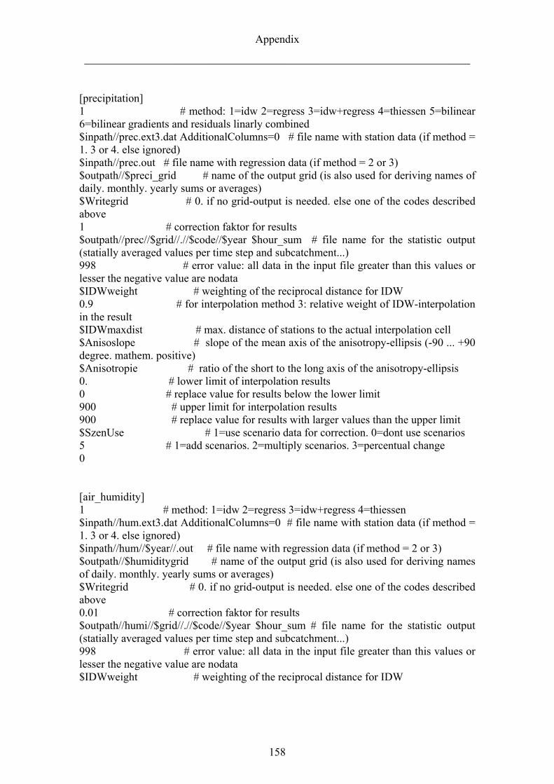
Appendix
_____________________________________________________________________
158
[precipitation] 1 # method: 1=idw 2=regress 3=idw+regress 4=thiessen 5=bilinear 6=bilinear gradients and residuals linarly combined $inpath//prec.ext3.dat AdditionalColumns=0 # file name with station data (if method = 1. 3 or 4. else ignored) $inpath//prec.out # file name with regression data (if method = 2 or 3) $outpath//$preci_grid # name of the output grid (is also used for deriving names of daily. monthly. yearly sums or averages) $Writegrid # 0. if no grid-output is needed. else one of the codes described above 1 # correction faktor for results $outpath//prec//$grid//.//$code//$year $hour_sum # file name for the statistic output (statially averaged values per time step and subcatchment...) 998 # error value: all data in the input file greater than this values or lesser the negative value are nodata $IDWweight # weighting of the reciprocal distance for IDW 0.9 # for interpolation method 3: relative weight of IDW-interpolation in the result $IDWmaxdist # max. distance of stations to the actual interpolation cell $Anisoslope # slope of the mean axis of the anisotropy-ellipsis (-90 ... +90 degree. mathem. positive) $Anisotropie # ratio of the short to the long axis of the anisotropy-ellipsis 0. # lower limit of interpolation results 0 # replace value for results below the lower limit 900 # upper limit for interpolation results 900 # replace value for results with larger values than the upper limit $SzenUse # 1=use scenario data for correction. 0=dont use scenarios 5 # 1=add scenarios. 2=multiply scenarios. 3=percentual change 0 [air_humidity] 1 # method: 1=idw 2=regress 3=idw+regress 4=thiessen $inpath//hum.ext3.dat AdditionalColumns=0 # file name with station data (if method = 1. 3 or 4. else ignored) $inpath//hum//$year//.out # file name with regression data (if method = 2 or 3) $outpath//$humiditygrid # name of the output grid (is also used for deriving names of daily. monthly. yearly sums or averages) $Writegrid # 0. if no grid-output is needed. else one of the codes described above 0.01 # correction faktor for results $outpath//humi//$grid//.//$code//$year $hour_sum # file name for the statistic output (statially averaged values per time step and subcatchment...) 998 # error value: all data in the input file greater than this values or lesser the negative value are nodata $IDWweight # weighting of the reciprocal distance for IDW
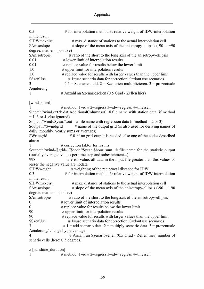
Appendix
_____________________________________________________________________
159
0.5 # for interpolation method 3: relative weight of IDW-interpolation in the result $IDWmaxdist # max. distance of stations to the actual interpolation cell $Anisoslope # slope of the mean axis of the anisotropy-ellipsis (-90 ... +90 degree. mathem. positive) $Anisotropie # ratio of the short to the long axis of the anisotropy-ellipsis 0.01 # lower limit of interpolation results 0.01 # replace value for results below the lower limit 1.0 # upper limit for interpolation results 1.0 # replace value for results with larger values than the upper limit $SzenUse # 1=use scenario data for correction. 0=dont use scenarios 3 # 1 = Szenarien add. 2 = Szenarien multiplizieren. 3 = prozentuale Aenderung 1 # Anzahl an Szenariozellen (0.5 Grad - Zellen hier) [wind_speed] 1 # method: 1=idw 2=regress 3=idw+regress 4=thiessen $inpath//wind.ext2b.dat AdditionalColumns=0 # file name with station data (if method = 1. 3 or 4. else ignored) $inpath//wind//$year//.out # file name with regression data (if method = 2 or 3) $outpath//$windgrid # name of the output grid (is also used for deriving names of daily. monthly. yearly sums or averages) $Writegrid # 0. if no grid-output is needed. else one of the codes described above 1 # correction faktor for results $outpath//wind//$grid//.//$code//$year $hour_sum # file name for the statistic output (statially averaged values per time step and subcatchment...) 998 # error value: all data in the input file greater than this values or lesser the negative value are nodata $IDWweight # weighting of the reciprocal distance for IDW 0.3 # for interpolation method 3: relative weight of IDW-interpolation in the result $IDWmaxdist # max. distance of stations to the actual interpolation cell $Anisoslope # slope of the mean axis of the anisotropy-ellipsis (-90 ... +90 degree. mathem. positive) $Anisotropie # ratio of the short to the long axis of the anisotropy-ellipsis 0 # lower limit of interpolation results 0 # replace value for results below the lower limit 90 # upper limit for interpolation results 90 # replace value for results with larger values than the upper limit $SzenUse # 1=use scenario data for correction. 0=dont use scenarios 3 # 1 = add scenario data. 2 = multiply scenario data. 3 = prozentuale Aenderung/ change by percentage 4 # Anzahl an Szenariozellen (0.5 Grad - Zellen hier) number of scnario cells (here: 0.5 degrees) # [sunshine_duration] 1 # method: 1=idw 2=regress 3=idw+regress 4=thiessen

Appendix
_____________________________________________________________________
160
$inpath//sun.ext2.dat AdditionalColumns=0 # file name with station data (if method = 1. 3 or 4. else ignored) $inpath//sun//$year//.out # file name with regression data (if method = 2 or 3) $outpath//$sunshinegrid # name of the output grid (is also used for deriving names of daily. monthly. yearly sums or averages) $Writegrid # 0. if no grid-output is needed. else one of the codes described above 1 # correction faktor for results $outpath//ssd_//$grid//.//$code//$year $hour_sum # file name for the statistic output (statially averaged values per time step and subcatchment...) 998 # error value: all data in the input file greater than this values or lesser the negative value are nodata $IDWweight # weighting of the reciprocal distance for IDW 0.5 # for interpolation method 3: relative weight of IDW-interpolation in the result $IDWmaxdist # max. distance of stations to the actual interpolation cell $Anisoslope # slope of the mean axis of the anisotropy-ellipsis (-90 ... +90 degree. mathem. positive) $Anisotropie # ratio of the short to the long axis of the anisotropy-ellipsis 0 # lower limit of interpolation results 0 # replace value for results below the lower limit 1.0 # upper limit for interpolation results 1.0 # replace value for results with larger values than the upper limit $SzenUse # 1=use scenario data for correction. 0=dont use scenarios 3 # 1 = add scenario data. 2 = multiply scenario data. 3 = prozentuale Aenderung/change by percentage 1 # Anzahl an Szenariozellen/number o f scenario cells (here: 0.5 Grad/degree – Zellen/cells hier) [global_radiation] 1 # method: 1=idw 2=regress 3=idw+regress 4=thiessen $inpath//rad.ext3.dat # file name with station data (if method = 1, 3 or 4, else ignored) $inpath//global//$year//.out # file name with regression data (if method = 2 or 3) $outpath//$radiationgrid # name of the output grid (is also used for deriving names of daily, monthly, yearly sums or averages) $Writegrid # 0, if no grid-output is needed, else one of the codes described above 1.0 # correction faktor for results $outpath//radiation_//$grid//.//$code//$year $hour_mean # file name for the statistic output (statially averaged values per time step and subcatchment...) 9998 # error value: all data in the input file greater than this values or lesser the negative value are nodata $IDWweight # weighting of the reciprocal distance for IDW 0.5 # for interpolation method 3: relative weight of IDW-interpolation in the result $IDWmaxdist # max. distance of stations to the actual interpolation cell $Anisoslope # slope of the mean axis of the anisotropy-ellipsis (-90 ... +90 degree, mathem. positive)

Appendix
_____________________________________________________________________
161
$Anisotropie # ratio of the short to the long axis of the anisotropy-ellipsis 0 # lower limit of interpolation results 0 # replace value for results below the lower limit 10000 # upper limit for interpolation results 10000 # replace value for results with larger values than the upper limit $SzenUse # 1=use scenario data for correction, 0=dont use scenarios # ---------- parameter for model components ----------------- # [precipitation_correction] 1 # 0=ignore this module. 1 = run the module 0.5 # Snow-rain-temperature 1.05 # liquid: b in: y = p(ax + b) 0.05 # liquid: a in: y = p(ax + b) = 1% more per m/s + 0.5% constant 1.10 # Snow: b in: y = p(ax + b) 0.13 # Snow: a in: y = p(ax + b) = 15% more per m/s + 45% constant # corretion factors for direct radiation are calculated # if the cell is in the shadow of another cell. or if a cell is not in the sun (slope angle!) # then the factor is 0. # control_parameter: 1 = radiation correction WITH shadow WITHOUT temperature correction # 2 = radiation correction WITH shadow WITH temperature correction # 3 = radiation correction WITHOUT shadow WITHOUT temperature correction. # 4 = radiation correction WITHOUT shadow WITH Temperatur [radiation_correction] 1 # 0=ignore this module. 1 = run the module $time # duration of a time step in minutes 2 # control parameter for radiation correction (see above) $outpath//$Tcorrgrid # name of the grids with the corrected temperatures $Writegrid # Writegrid for corrected temperatures 5 # factor x for temperature correction x * (-1.6 .... +1.6) $outpath//$ExpoCorrgrid # name of the grids with the correction factors for the direct radiation $Writegrid # Writegrid $outpath//$Shapegrid # name of the grids for codes 1 for theor. shadow. 0 for theor. no shadow (day; assumed: SSD=1.0) $Writegrid # Writegrid 1 # interval counter. after reaching this value. a new correction is calculated (3=all 3 hours a.s.o.) 1 # Spitting of the interval. usefull for time step=24 hours (then: split=24. -> each hour one correction calculation) [evapotranspiration]
Appendix
_____________________________________________________________________
162
1 # 0=ignore this module. 1 = run the module $time # duration of a time step in minutes 1 # Method: 1=Penman-Monteith. 2=Hamon (only daily). 3=Wendling (only daily) 4= Haude (only daily) 0.5 0.6 0.8 1.0 1.1 1.1 1.2 1.1 1.0 0.9 0.7 0.5 # PEC correction factor for HAMON-evapotranspiration 0.20 0.20 0.21 0.29 0.29 0.28 0.26 0.25 0.22 0.22 0.20 0.20 # fh (only for method 4: Haude) monthly values (Jan ... Dec) (here: for Grass) 0.5 # fk -> factor for Wendling-evapotranspiration (only for Method = 3) $outpath//$ETPgrid # result grid for potential evapotranspiration in mm/dt $Writegrid # 0. if no grid-output is needed. else one of the codes described above $outpath//etp_//$grid//.//$code//$year $hour_sum # statisticfile for subcatchments (zones) of the potential evapotranspiration $outpath//$ETRgrid # result grid for real evapotranspiration in mm/dt $Writegrid # 0. if no grid-output is needed. else one of the codes described above $outpath//etr_//$grid//.//$code//$year $hour_sum # statistic for subcatchments (zones) of the real evapotranspiration $outpath//$EVAPgrid # result grid for real evapotranspiration in mm/dt $Writegrid # 0. if no grid-output is needed. else one of the codes described above $outpath//evap//$grid//.//$code//$year $hour_sum # statistic for subcatchments (zones) of the potential evaporation $outpath//$EVARgrid # result grid for real evapotranspiration in mm/dt $Writegrid # 0. if no grid-output is needed. else one of the codes described above $outpath//evar//$grid//.//$code//$year $hour_sum # statistic for subcatchments (zones) of the real evaporation $outpath//$ETRSgrid # result grid for real snow evapotranspiration in mm/dt $Writegrid # 0. if no grid-output is needed. else one of the codes described above $outpath//etrs//$grid//.//$code//$year $hour_sum # statistic for subcatchments (zones) of the real snow evaporation $outpath//$EIPgrid # result grid for pot. interception evaporation in mm/dt $Writegrid # 0. if no grid-output is needed. else one of the codes described above $outpath//eip_//$grid//.//$code//$year $hour_sum # statisticfile for zones of pot. interception evaporation $outpath//rgex//$grid//.//$code//$year $hour_sum # statistic for subcatchments (zones) of the corrected radiation +0.23 +1.77 -2.28 +1.28 # coefficients c for Polynom of order 3 RG = c1 + c2*SSD + c3*SSD^2 + c4*SSD^3 +0.072 -0.808 +2.112 -0.239 # coefficients x for Polynom of order 3 SSD = x1 + x2*RG + x3*RG^2 + x4*RG^3 0.88 0.05 # Extinktion coefficient for RG-modeling (Phi and dPhi) (summer phi = phi-dphi. winter phi=phi+dphi) 1654.0 # recession constant (e-function for recession of the daily temperature amplitude with altitude [m]
Appendix
_____________________________________________________________________
163
3.3 4.4 6.1 7.9 9.4 10.0 9.9 9.0 7.8 6.0 4.2 3.2 # monthly values of the max. daily T-amplitudes (for 0 m.a.s.l) 0.62 0.1 # part of the temperature amplitude (dt). that is added to the mean day-temperature # (followed by the range of changing within a year ddt) to get the mean temperature of light day # in the night: mean night temperature is mean day temperature minus (1-dt)*(temp. amplitude) [snow_model] 0 # 0=ignore this module. 1 = run the module $time # duration of a time step in minutes 1 # method 1=T-index. 2=t-u-index. 3=Anderson comb.. 4=extended com. 1 # transient zone for rain-snow (T0R +- this range) 0.5 # T0R temperature limit for rain (Grad Celsius) -0.5 # T0 temperature limit snow melt 0.1 # CWH storage capacity of the snow for water (relative part) 1.0 # CRFR coefficient for refreezing 2.0 # C0 degree-day-factor mm/d/C 1.8 # C1 degree-day-factor without wind consideration mm/(d*C) 0.8 # C2 degree-day-factor considering wind mm/(d*C*m/s) 0.07 # z0 roughness length cm for energy bilance methods (not used) 1.5 # RMFMIN minimum radiation melt factor mm/d/C comb. method 2.5 # RMFMAX maximum radiation melt factor mm/d/C comb. method 0.40 # Albedo for snow (Min) 0.85 # Albedo for snow (Max) $outpath//$rain_rate # rain rate $Writegrid # 0. if no grid-output is needed. else one of the codes described above $outpath//rain//$grid//.//$code//$year $hour_sum # rain rate $outpath//$snow_rate # snow rate $Writegrid # 0. if no grid-output is needed. else one of the codes described above $outpath//snow//$grid//.//$code//$year $hour_sum # snow rate $outpath//$days_snow # number of days with snow (SWE > 5mm) $Writegrid # 0. if no grid-output is needed. else one of the codes described above $outpath//sday//$grid//.//$code//$year $hour_sum # number of days with snow (SWE > 5mm) $outpath//$snow_age # snow age (days without new snow) $Writegrid # 0. if no grid-output is needed. else one of the codes described above $outpath//sage//$grid//.//$code//$year $hour_sum # days since last snowfall $outpath//albe//$grid//.//$code//$year $hour_sum # Albedo $outpath//$snowcover_outflow # discharge from snow. input (precipitation) for following modules

Appendix
_____________________________________________________________________
164
$Writegrid # 0. if no grid-output is needed. else one of the codes described above $outpath//qsch//$grid//.//$code//$year $hour_sum # melt flow (or rain. if there is no snow cover) in mm/dt $outpath//$melt_from_snowcover # discharge from snow. input (precipitation) for following modules $Writegrid # 0. if no grid-output is needed. else one of the codes described above $outpath//qsme//$grid//.//$code//$year $hour_sum # melt flow in mm/dt $outpath//$SSNOgrid # name of the grids with the snow storage solid in mm $Writegrid # 0. if no grid-output is needed. else one of the codes described above $outpath//$SLIQgrid # name of the grids with the snow storage liquid in mm $Writegrid # 0. if no grid-output is needed. else one of the codes described above $outpath//ssto//$grid//.//$code//$year $hour_sum # total snow storage. in mm. (liquid and solid fraction) $outpath//$SSTOgrid # name of the grids with the total snow storage solid AND liquid in mm $Writegrid # 0. if no grid-output is needed. else one of the codes described above $readgrids # 1=read snow storage solid. liquid grids from disk. 0=generate new grids [ice_firn] 2 # method for glacier melt: 1=classical t-index. 2=t-index with correction by radiation 5 # t-index factor for ice 4 # t-index factor for firn 3 # t-index factor for snow 2 # melt factor 0.0001 # radiation coefficient for ice_min (for method 2) 0.0007 # radiation coefficient for ice_max (for method 2) 0.0001 # radiation coefficient for snow_min (for method 2) 0.00055 # radiation coefficient for snow_max (for method 2) 40 # els-konstante for ice 350 # els-konstante for firn 120 # els-konstante for snow 0.0006 # initial reservoir content for ice discharge (single linear storage approach) 0.0006 # initial reservoir content for firn discharge (single linear storage approach) 0.0006 # initial reservoir content for snow discharge (single linear storage approach) $outpath//$firn_melt # melt from firn $Writegrid # 0, if no grid-output is needed, else one of the codes described above $outpath//qfir//$grid//.//$code//$year $hour_mean # melt from firn as statistic file $outpath//$ice_melt # melt from ice $Writegrid # 0, if no grid-output is needed, else one of the codes described above $outpath//qice//$grid//.//$code//$year $hour_mean # melt from ice as statistic file
Appendix
_____________________________________________________________________
165
$outpath//qglc//$grid//.//$code//$year $hour_mean # discharge from snow, ice and firn as statistic file [interception_model] 1 # 0=ignore this module. 1 = run the module $time # duration of a time step in minutes 2 # method: 1 = use ETP for calculating EI; 2 = use EIP for calculating EI (only effective for method 1 in evapotranspiration model -> for other methods. ETP = EIP) $outpath//$throughfall # result grid : = outflow from the interception storage $Writegrid # 0. if no grid-output is needed. else one of the codes described above $outpath//qi__//$grid//.//$code//$year $hour_sum # statistic file interception storage outflow $outpath//$EIgrid # Interzeption evaporation. grid $Writegrid # 0. if no grid-output is needed. else one of the codes described above $outpath//ei__//$grid//.//$code//$year $hour_sum # zonal statistic $outpath//$SIgrid # storage content of the interception storage $Writegrid # 0. if no grid-output is needed. else one of the codes described above $outpath//si__//$grid//.//$code//$year $hour_sum # zonal statistic For interception storage content 0.35 # layer thickness of the waters on the leaves (multiplied with LAI -> storage capacity) $readgrids # 1=read grids from disk. else generate internal [infiltration_model] 0 # 0=ignore this module. 1 = run the module $time # duration of a time step in minutes [unsatzon_model] 1 # 0=ignore this module. 1 = run the module $time # duration of a time step in minutes 3 # method, 1=simple method (will not work anymore from version 7.x), 2 = FDM-Method 3 = FDM-Method with dynamic time step down to 1 secound 2 # controlling interaction with surface water: 0 = no interaction. 1 = exfiltration possible 2 = infiltration and exfiltration possible 0 # controlling surface storage in ponds: 0 = no ponds. 1 = using ponds for surface storage (pond depth as standard grid needed -> height of dams oround fields) 0 # controlling artificial drainage: 0 = no artificial drainage 1 = using drainage (drainage depth and horizontal pipe distances as standard grids needed!) 0 # controlling clay layer: 0 = no clay layer. 1 = assuming a clay layer in a depth. specified within a clay-grid (declared as a standard grid)
Appendix
_____________________________________________________________________
166
5e-8 # permeability of the clay layer (is used for the clay layer only) 4 # parameter for the initialization of the gw_level (range between 1..levels (standard: 4)) $outpath//qdra//$grid//.//$code//$year $hour_sum # results drainage discharge in mm per zone $outpath//gwst//$grid//.//$code//$year $hour_sum # results groundwater depth $outpath//gwn_//$grid//.//$code//$year $hour_sum # results mean groundwater recharge per zone $outpath//sb05//$grid//.//$code//$year $hour_sum # results rel. soil moisture within the root zone per zone $outpath//sb1_//$grid//.//$code//$year $hour_sum # results rel. soil moisture within the unsat. zone (0m..GW table) per zone $outpath//wurz//$grid//.//$code//$year $hour_sum # results statistic of the root depth per zone $outpath//infx//$grid//.//$code//$year $hour_sum # results statistic of the infiltration excess $outpath//pond//$grid//.//$code//$year $hour_sum # results statistic of the ponding water storage content $outpath//qdir//$grid//.//$code//$year $hour_sum # results statistic of the direct discharge $outpath//qifl//$grid//.//$code//$year $hour_sum # results statistic of the interflow $outpath//qbas//$grid//.//$code//$year $hour_sum # results statistic of the baseflow $outpath//qges//$grid//.//$code//$year $hour_sum # results statistic of the total discharge $outpath//gwin//$grid//.//$code//$year $hour_sum # statistic of the infiltration from surface water into groundwater (from rivers and lakes) $outpath//gwex//$grid//.//$code//$year $hour_sum # statistic of the exfiltration from groundwater into surface water (into rivers and lakes) $outpath//macr//$grid//.//$code//$year $hour_sum # statistic of infiltration into macropores $outpath//qinf//$grid//.//$code//$year $hour_sum # statistic of total infiltration into the first soil layer $outpath//$SB_1_grid # grid with actual soil water content for the root zone $Writegrid # writegrid for this grid $outpath//$SB_2_grid # grid with actual soil water content for the root zone $Writegrid # writegrid for this grid $outpath//$ROOTgrid # grid with root depth $Writegrid # writegrid for this grid $outpath//$Thetastack # stack. actual soil water content for all soil levels $Writestack # Writecode for this stack $outpath//$hydraulic_heads_stack # stack. contaiing hydraulic heads $Writestack # Writecode for this stack $outpath//$geodetic_altitude_stack # stack. containig geodaetic altitudes of the soil levels (lower boudaries) $Writestack # Writecode for this stack $outpath//$flowstack # stack. containing the outflows from the soil levels $Writestack # Writecode for this stack $outpath//$GWdepthgrid # grid with groudwaterdepth $Writegrid # writegrid for this grid
Appendix
_____________________________________________________________________
167
$outpath//$GWthetagrid # grid with theta in GWLEVEL $Writegrid # writegrid for this grid $outpath//$GWNgrid # grid with groundwater recharge $Writegrid # writegrid for this grid $outpath//$GWLEVELgrid # grid with level index of groundwater surface (Index der Schicht) $Writegrid # writegrid for this grid $outpath//$QDRAINgrid # grid with the drainage flows $Writegrid # writegrid for this grid $outpath//$SATTgrid # grid with code 1=saturation at interval start. 0 no sat. $Writegrid # writegrid for this grid $outpath//$INFEXgrid # grid with infiltration excess in mm (surface discharge) $Writegrid # writegrid for this grid $outpath//$QDgrid # grid with direct discharge $Writegrid # writegrid for this grid $outpath//$QIgrid # grid with Interflow $Writegrid # writegrid for this grid $outpath//$QBgrid # grid with baseflow $Writegrid # writegrid for this grid $outpath//$GWINgrid # grid with infiltration from rivers into the soil (groundwater) $Writegrid # writegrid for re-infiltration $outpath//$GWEXgrid # grid with exfiltration (baseflow) from groundwater (is only generated. if groundwater module is active. else baseflow is in QBgrid) $Writegrid # writegrid for exfiltration $outpath//$act_pond_grid # grid with content of ponding storge $Writegrid # writegrid for this grid $outpath//$UPRISEgrid # grid with amount of capillary uprise (mm) $Writegrid # writegrid for this grid $outpath//$PERCOLgrid # grid with amount of percolation (mm) $Writegrid # writegrid for this grid $outpath//$MACROINFgrid # grid with amount of infiltration into macropores (mm) $Writegrid # writegrid for this grid 500 500 # coordinates of control plot. all theta and qu-values are written to files (qu.dat. theta.dat in the directory. from which the model is started) $outpath//qbot//$grid//.//$code//$year # name of a file containing the flows between the layers of the control point $outpath//thet//$grid//.//$code//$year # name of a file containing the soil moisture as theta values of the layers of the control point $outpath//hhyd//$grid//.//$code//$year # name of a file containing the hydraulic head of the layers of the control point $outpath//otherdata//$grid//.//$code//$year # name of a file containing some other water balance data of the control point (non layer data) $outpath//etrd//$grid//.//$code//$year # name of a file containing the water withdrawal by evaporation and transpiration for each layer of the control point $outpath//intd//$grid//.//$code//$year # name of a file containing the interflow rate for each layer of the control point 1 6 11 15 16 18 # range for subbasin codes
Appendix
_____________________________________________________________________
168
500 350 10 100 150 10 # kelsqd 600 300 20 200 200 20 # kelsqi 2 50 12 200 20 3 # drainage density 0.4 0.4 0.4 0.4 0.4 0.4 # k in qb = Q0 * exp(-k/z) with z = depth to groundwater 0.65 0.65 0.65 0.65 0.65 0.65 # Q0 in the above formula 0.1 0.1 0.1 0.1 0.1 0.1 # fraction of surface runoff on snow melt $readgrids # meanings are extended now! read the follwing comments $outpath//storage.ftz # if readgrids = 1. then this file contains the contents of the flow travel time zones for interflow and surface flow and for the tracers 60 # minimum dynamic time step in secounds. the smaller this number, the longer the model runs but the results will be more accurate due to a maintained Courant condition $outpath//step//$grid//.//$code//$year $hour_mean # results statistic of the number of substeps $outpath//$SUBSTEPSgrid # grid with number of substeps --> a good idea is to use writecode 5x (e.g. 53) to get the average number of substeps per cell for the model run 5//$Writegrid # for substeps, the areal distribution is of interest for the annual average value. This is code 6 as first digit in 2-digit codes. Or use 5 for the entire model run [irrigation] 0 # 0=ignore this module. 1 = run the module $time # duration of a time step in minutes [groundwater_flow] 0 # 0=ignore the module. 1 = run the module $time # duration of a time step in minutes; doen't change the value unless you have strong reasons to do so!! [soil_model] 1 # 0=ignore this module. 1 = run the module $time # duration of a time step in minutes [routing_model] 1 # 0=ignore this module. 1 = run the module. 2=run the module with observed inflows into the routing channels (from discharge files) $time # duration of a time step in minutes 0.01 100 90 24 # minimum/maximum specific discharge (l/s/km^2). number of log. fractions of the range. splitting of the timeintervall (24= 1 hour-intervalls are splitted into 24 Intervalls each of 2.5 min. duration) $outpath//qgko//$grid//.//$code//$year $routing_code # name of the statistic file with routed discharges $inpath//spend.dat # name of the file with observed discharges (mm/Timestep or m^3/s)
Appendix
_____________________________________________________________________
169
1 # number of following column descripotr (which column in the spec. disch. file corresponds to which subbasin 1 1 # first number: subbasin. second: column index 720 # timeoffset (for r-square calculation. intervals up to this parameter are not evaluated in r-square calculation. e.g. 12: first 12 intervals are neglected ) TG 2 (AE=75415.000, AErel=1.0) from OL 15 (kh=0.1, kv=0.4, Bh=19.0, Bv= 75.9, Th= 1.90, Mh=30.0, Mv=12.0, I=0.0010, L=314082.8, AE=232.000) and OL 5 (kh=0.1, kv=0.4, Bh= 6.6, Bv= 26.5, Th= 0.66, Mh=30.0, Mv=12.0, I=0.0010, L=243112.4, AE=14.000) TG 11 (AE=56760.000, AErel=1.0) from OL 13 (kh=0.1, kv=0.4, Bh=131.2, Bv=524.6, Th=13.12, Mh=30.0, Mv=12.0, I=0.0010, L=128183.4, AE=40180.000) and OL 12 (kh=0.1, kv=0.4, Bh=82.1, Bv=328.4, Th= 8.21, Mh=30.0, Mv=12.0, I=0.0010, L=78627.2, AE=11522.000) TG 6 (AE=94040.000, AErel=1.0) from OL 10 (kh=0.1, kv=0.4, Bh=79.8, Bv=319.0, Th= 7.98, Mh=30.0, Mv=12.0, I=0.0010, L=138810.6, AE=10667.000) and OL 11 (kh=0.1, kv=0.4, Bh=149.3, Bv=597.2, Th=14.93, Mh=30.0, Mv=12.0, I=0.0010, L=158739.6, AE=56760.000) and OL 9 (kh=0.1, kv=0.4, Bh=80.0, Bv=319.8, Th= 8.00, Mh=30.0, Mv=12.0, I=0.0010, L=135982.2, AE=10737.000) and OL 8 (kh=0.1, kv=0.4, Bh=58.2, Bv=232.7, Th= 5.82, Mh=30.0, Mv=12.0, I=0.0010, L=92284.0, AE=4598.000) and OL 7 (kh=0.1, kv=0.4, Bh=13.6, Bv= 54.3, Th= 1.36, Mh=30.0, Mv=12.0, I=0.0010, L=53142.0, AE=95.000) TG 4 (AE=109142.000, AErel=1.0) from OL 6 (kh=0.1, kv=0.4, Bh=180.4, Bv=721.7, Th=18.04, Mh=30.0, Mv=12.0, I=0.0010, L=154396.4, AE=94040.000) TG 17 (AE=143233.000, AErel=1.0) from OL 18 (kh=0.1, kv=0.4, Bh=188.2, Bv=752.9, Th=18.82, Mh=30.0, Mv=12.0, I=0.0010, L=351260.2, AE=105259.000) TG 16 (AE=143850.000, AErel=1.0) from OL 17 (kh=0.1, kv=0.4, Bh=211.3, Bv=845.0, Th=21.13, Mh=30.0, Mv=12.0, I=0.0010, L=13656.8, AE=143233.000) TG 3 (AE=153914.000, AErel=1.0) from OL 16 (kh=0.1, kv=0.4, Bh=211.6, Bv=846.4, Th=21.16, Mh=30.0, Mv=12.0, I=0.0010, L=206005.8, AE=143850.000) TG 1 (AE=402990.000, AErel=1.0) from OL 2 (kh=0.1, kv=0.4, Bh=166.1, Bv=664.4, Th=16.61, Mh=30.0, Mv=12.0, I=0.0010, L=123798.8, AE=75415.000) and OL 4 (kh=0.1, kv=0.4, Bh=190.8, Bv=763.1, Th=19.08, Mh=30.0, Mv=12.0, I=0.0010, L=329059.0, AE=109142.000) and OL 3 (kh=0.1, kv=0.4, Bh=217.0, Bv=868.1, Th=21.70, Mh=30.0, Mv=12.0, I=0.0010, L=329059.0, AE=153914.000) [abstraction_rule_reservoir_1]
Appendix
_____________________________________________________________________
170
0 [multilayer_landuse] 1 # count of multilayer landuses 1 grass_variable { Landuse_Layers = 7, -9999, -9999; k_extinct = 0.3; LAI_scale = 20;} [landuse_table] 9 # number of following land use codes 6 crop.wood.mos_variable {method = VariableDayCount; # valid methods: "VariableDayCount" with variable number of fix points (other methods will follow) --> old method: if the table is structured like the old ones, they are still valid RootDistr = 1.0; # parameter for root density distribution TReduWet = 0.95; # relative Theta value for beginning water stress (under wet conditions -> set >= 1 for crop which doesn't depend on an aeral zone LimitReduWet = 0.5; # minimum relative reduction factor of real transpiration when water content reaches saturation. The reduction factor value will go down linearly starting at 1.0 when relative Theta equals TReduWet (e.g. 0.95) to LimitReduWet when the soil is saturated (Theta rel = 1.0) HReduDry = 3.45; # hydraulic head (suction) for beginning dryness stress (for water content resulting in higher suctions, ETR will be reduced down to 0 at suction=150m) IntercepCap = 0.2; # optional: specific thickness of the water layer on the leafes in mm. if omitted here, the dedfault parameter from interception_model is used JulDays = 120 304; # Julian days for all following rows. Each parameter must match the number of julian days given here! The count of days doesn't matter. Albedo = 0.16 0.16; # Albedo (snow free) rsc = 80 80 70 70 50 50 50 55 55 70 80 80; # leaf surface resistance in s/m rs_interception = 80 80 70 70 50 50 50 55 55 70 80 80; # INTERCEPTION surface resistance in s/m rs_evaporation = 250 250 250 250 250 250 250 250 250 250 250 250; # SOIL surface resistance in s/m (for evaporation only) LAI = 3 5; # Leaf Area Index (1/1) Z0 = 1.5 2.5; # Roughness length in m VCF = 0.9 0.95; # Vegetation covered fraction ("Vegetationsbedeckungsgrad") RootDepth = 0.5 0.5; # Root depth in m AltDep = 0.025 0.025 0.025 0.025 0.025 0.025 -0.025 -0.025 -0.025 -0.025 -0.025 -0.025; # Verschiebung des Juldays pro Meter (positiv: wird nach hinten geschoben, negativ: wird nach vorne geschoben -> Limit: Wenn zwei Punkte aufeinandertreffen, dann wird nicht weiter verschoben) Julian day shift per meter (positive: backward shift, negative: forward shift, limit: no further shift with two converging values. }
Appendix
_____________________________________________________________________
171
7 grass_variable {method = VariableDayCount; # valid methods: "VariableDayCount" with variable number of fix points (other methods will follow) --> old method: if the table is structured like the old ones, they are still valid RootDistr = 1.0; # parameter for root density distribution TReduWet = 0.95; # relative Theta value for beginning water stress (under wet conditions -> set >= 1 for crop which doesn't depend on an aeral zone LimitReduWet = 0.5; # minimum relative reduction factor of real transpiration when water content reaches saturation. The reduction factor value will go down linearly starting at 1.0 when relative Theta equals TReduWet (e.g. 0.95) to LimitReduWet when the soil is saturated (Theta rel = 1.0) HReduDry = 3.45; # hydraulic head (suction) for beginning dryness stress (for water content resulting in higher suctions, ETR will be reduced down to 0 at suction=150m) IntercepCap = 0.2; # optional: specific thickness of the water layer on the leafes in mm. if omitted here, the dedfault parameter from interception_model is used JulDays = 120 304; # Julian days for all following rows. Each parameter must match the number of julian days given here! The count of days doesn't matter. Albedo = 0.19 0.19; # Albedo (snow free) rsc = 90 90 75 65 50 55 55 55 60 70 90 90; # leaf surface resistance in s/m rs_interception = 90 90 75 65 50 55 55 55 60 70 90 90; # INTERCEPTION surface resistance in s/m rs_evaporation = 250 250 250 250 250 250 250 250 250 250 250 250; # SOIL surface resistance in s/m (for evaporation only) LAI = 2 4; # Leaf Area Index (1/1) Z0 = 0.15 0.4; # Roughness length in m VCF = 0.95 0.95; # Vegetation covered fraction ("Vegetationsbedeckungsgrad") RootDepth = 0.4 0.4; # Root depth in m AltDep = 0.025 0.025 0.025 0.025 0.025 0.025 -0.025 -0.025 -0.025 -0.025 -0.025 -0.025; # Verschiebung des Juldays pro Meter (positiv: wird nach hinten geschoben, negativ: wird nach vorne geschoben -> Limit: Wenn zwei Punkte aufeinandertreffen, dann wird nicht weiter verschoben) Julian day shift per meter (positive: backward shift, negative: forward shift, limit: no further shift with two converging values.) } 8 shrubland_variable {method = VariableDayCount; # valid methods: "VariableDayCount" with variable number of fix points (other methods will follow) --> old method: if the table is structured like the old ones, they are still valid RootDistr = 1.0; # parameter for root density distribution TReduWet = 0.95; # relative Theta value for beginning water stress (under wet conditions -> set >= 1 for crop which doesn't depend on an aeral zone LimitReduWet = 0.5; # minimum relative reduction factor of real transpiration when water content reaches saturation. The reduction factor value will go down linearly starting at 1.0 when relative Theta equals TReduWet (e.g. 0.95) to LimitReduWet when the soil is saturated (Theta rel = 1.0)
Appendix
_____________________________________________________________________
172
HReduDry = 3.45; # hydraulic head (suction) for beginning dryness stress (for water content resulting in higher suctions, ETR will be reduced down to 0 at suction=150m) IntercepCap = 0.2; # optional: specific thickness of the water layer on the leafes in mm. if omitted here, the dedfault parameter from interception_model is used JulDays = 120 304; # Julian days for all following rows. Each parameter must match the number of julian days given here! The count of days doesn't matter. Albedo = 0.22 0.22; # Albedo (snow free) rsc = 80 80 70 70 50 50 50 55 55 70 80 80; # leaf surface resistance in s/m rs_interception = 80 80 70 70 50 50 50 55 55 70 80 80; # INTERCEPTION surface resistance in s/m rs_evaporation = 250 250 250 250 250 250 250 250 250 250 250 250; # SOIL surface resistance in s/m (for evaporation only) LAI = 3 5; # Leaf Area Index (1/1) Z0 = 1.5 2.5; # Roughness length in m VCF = 0.9 0.95; # Vegetation covered fraction ("Vegetationsbedeckungsgrad") RootDepth = 0.5 0.5; # Root depth in m AltDep = 0.025 0.025 0.025 0.025 0.025 0.025 -0.025 -0.025 -0.025 -0.025 -0.025 -0.025; # Verschiebung des Juldays pro Meter (positiv: wird nach hinten geschoben, negativ: wird nach vorne geschoben -> Limit: Wenn zwei Punkte aufeinandertreffen, dann wird nicht weiter verschoben) Julian day shift per meter (positive: backward shift, negative: forward shift, limit: no further shift with two converging values.) } 10 savanna_variable {method = VariableDayCount; # valid methods: "VariableDayCount" with variable number of fix points (other methods will follow) --> old method: if the table is structured like the old ones, they are still valid RootDistr = 1.0; # parameter for root density distribution TReduWet = 0.95; # relative Theta value for beginning water stress (under wet conditions -> set >= 1 for crop which doesn't depend on an aeral zone LimitReduWet = 0.5; # minimum relative reduction factor of real transpiration when water content reaches saturation. The reduction factor value will go down linearly starting at 1.0 when relative Theta equals TReduWet (e.g. 0.95) to LimitReduWet when the soil is saturated (Theta rel = 1.0) HReduDry = 3.45; # hydraulic head (suction) for beginning dryness stress (for water content resulting in higher suctions, ETR will be reduced down to 0 at suction=150m) IntercepCap = 0.2; # optional: specific thickness of the water layer on the leafes in mm. if omitted here, the dedfault parameter from interception_model is used JulDays = 120 304; # Julian days for all following rows. Each parameter must match the number of julian days given here! The count of days doesn't matter. Albedo = 0.2 0.2; # Albedo (snow free)
Appendix
_____________________________________________________________________
173
rsc = 80 80 70 70 50 50 50 55 55 70 80 80; # leaf surface resistance in s/m rs_interception = 80 80 70 70 50 50 50 55 55 70 80 80; # INTERCEPTION surface resistance in s/m rs_evaporation = 250 250 250 250 250 250 250 250 250 250 250 250; # SOIL surface resistance in s/m (for evaporation only) LAI = 3 5; # Leaf Area Index (1/1) Z0 = 1.5 2.5; # Roughness length in m VCF = 0.9 0.95; # Vegetation covered fraction ("Vegetationsbedeckungsgrad") RootDepth = 0.5 0.5; # Root depth in m AltDep = 0.025 0.025 0.025 0.025 0.025 0.025 -0.025 -0.025 -0.025 -0.025 -0.025 -0.025; # Verschiebung des Juldays pro Meter (positiv: wird nach hinten geschoben, negativ: wird nach vorne geschoben -> Limit: Wenn zwei Punkte aufeinandertreffen, dann wird nicht weiter verschoben) Julian day shift per meter (positive: backward shift, negative: forward shift, limit: no further shift with two converging values.) } 11 decids.Broadl_variable {method = VariableDayCount; # valid methods: "VariableDayCount" with variable number of fix points (other methods will follow) --> old method: if the table is structured like the old ones, they are still valid RootDistr = 1.0; # parameter for root density distribution TReduWet = 0.95; # relative Theta value for beginning water stress (under wet conditions -> set >= 1 for crop which doesn't depend on an aeral zone LimitReduWet = 0.5; # minimum relative reduction factor of real transpiration when water content reaches saturation. The reduction factor value will go down linearly starting at 1.0 when relative Theta equals TReduWet (e.g. 0.95) to LimitReduWet when the soil is saturated (Theta rel = 1.0) HReduDry = 3.45; # hydraulic head (suction) for beginning dryness stress (for water content resulting in higher suctions, ETR will be reduced down to 0 at suction=150m) IntercepCap = 0.2; # optional: specific thickness of the water layer on the leafes in mm. if omitted here, the dedfault parameter from interception_model is used JulDays = 120 304; # Julian days for all following rows. Each parameter must match the number of julian days given here! The count of days doesn't matter. Albedo = 0.16 0.16; # Albedo (snow free) rsc = 100 100 95 75 65 65 65 65 65 85 100 100; # leaf surface resistance in s/m rs_interception = 100 100 95 75 65 65 65 65 65 85 100 100; # INTERCEPTION surface resistance in s/m rs_evaporation = 250 250 250 250 250 250 250 250 250 250 250 250; # SOIL surface resistance in s/m (for evaporation only) LAI = 0.5 8; # Leaf Area Index (1/1) Z0 = 0.3 10; # Roughness length in m VCF = 0.7 0.95; # Vegetation covered fraction ("Vegetationsbedeckungsgrad")
Appendix
_____________________________________________________________________
174
RootDepth = 1.4 1.4; # Root depth in m AltDep = 0.025 0.025 0.025 0.025 0.025 0.025 -0.025 -0.025 -0.025 -0.025 -0.025 -0.025; # Verschiebung des Juldays pro Meter (positiv: wird nach hinten geschoben, negativ: wird nach vorne geschoben -> Limit: Wenn zwei Punkte aufeinandertreffen, dann wird nicht weiter verschoben) Julian day shift per meter (positive: backward shift, negative: forward shift, limit: no further shift with two converging values.) } 13 evergreen.broadl_variable {method = VariableDayCount; # valid methods: "VariableDayCount" with variable number of fix points (other methods will follow) --> old method: if the table is structured like the old ones, they are still valid RootDistr = 1.0; # parameter for root density distribution TReduWet = 0.95; # relative Theta value for beginning water stress (under wet conditions -> set >= 1 for crop which doesn't depend on an aeral zone LimitReduWet = 0.5; # minimum relative reduction factor of real transpiration when water content reaches saturation. The reduction factor value will go down linearly starting at 1.0 when relative Theta equals TReduWet (e.g. 0.95) to LimitReduWet when the soil is saturated (Theta rel = 1.0) HReduDry = 3.45; # hydraulic head (suction) for beginning dryness stress (for water content resulting in higher suctions, ETR will be reduced down to 0 at suction=150m) IntercepCap = 0.2; # optional: specific thickness of the water layer on the leafes in mm. if omitted here, the dedfault parameter from interception_model is used JulDays = 120 304; # Julian days for all following rows. Each parameter must match the number of julian days given here! The count of days doesn't matter. Albedo = 0.12 0.12; # Albedo (snow free) rsc = 65 65 65 65 65 65 65 65 65 65 65 65; # leaf surface resistance in s/m rs_interception = 65 65 65 65 65 65 65 65 65 65 65 65; # INTERCEPTION surface resistance in s/m rs_evaporation = 250 250 250 250 250 250 250 250 250 250 250 250; # SOIL surface resistance in s/m (for evaporation only) LAI = 8 8; # Leaf Area Index (1/1) Z0 = 10 10; # Roughness length in m VCF = 0.95 0.95; # Vegetation covered fraction ("Vegetationsbedeckungsgrad") RootDepth = 1.4 1.4; # Root depth in m AltDep = 0.025 0.025 0.025 0.025 0.025 0.025 -0.025 -0.025 -0.025 -0.025 -0.025 -0.025; # Verschiebung des Juldays pro Meter (positiv: wird nach hinten geschoben, negativ: wird nach vorne geschoben -> Limit: Wenn zwei Punkte aufeinandertreffen, dann wird nicht weiter verschoben) Julian day shift per meter (positive: backward shift, negative: forward shift, limit: no further shift with two converging values.) }
Appendix
_____________________________________________________________________
175
15 mixed.forest_variable {method = VariableDayCount; # valid methods: "VariableDayCount" with variable number of fix points (other methods will follow) --> old method: if the table is structured like the old ones, they are still valid RootDistr = 1.0; # parameter for root density distribution TReduWet = 0.95; # relative Theta value for beginning water stress (under wet conditions -> set >= 1 for crop which doesn't depend on an aeral zone LimitReduWet = 0.5; # minimum relative reduction factor of real transpiration when water content reaches saturation. The reduction factor value will go down linearly starting at 1.0 when relative Theta equals TReduWet (e.g. 0.95) to LimitReduWet when the soil is saturated (Theta rel = 1.0) HReduDry = 3.45; # hydraulic head (suction) for beginning dryness stress (for water content resulting in higher suctions, ETR will be reduced down to 0 at suction=150m) IntercepCap = 0.2; # optional: specific thickness of the water layer on the leafes in mm. if omitted here, the dedfault parameter from interception_model is used JulDays = 120 304; # Julian days for all following rows. Each parameter must match the number of julian days given here! The count of days doesn't matter. Albedo = 0.13 0.13; # Albedo (snow free) rsc = 90 90 85 70 60 60 60 60 60 80 90 90; # leaf surface resistance in s/m rs_interception = 90 90 85 70 60 60 60 60 60 80 90 90; # INTERCEPTION surface resistance in s/m rs_evaporation = 250 250 250 250 250 250 250 250 250 250 250 250; # SOIL surface resistance in s/m (for evaporation only) LAI = 2 10; # Leaf Area Index (1/1) Z0 = 3 10; # Roughness length in m VCF = 0.8 0.92; # Vegetation covered fraction ("Vegetationsbedeckungsgrad") RootDepth = 1.3 1.3; # Root depth in m AltDep = 0.025 0.025 0.025 0.025 0.025 0.025 -0.025 -0.025 -0.025 -0.025 -0.025 -0.025; # Verschiebung des Juldays pro Meter (positiv: wird nach hinten geschoben, negativ: wird nach vorne geschoben -> Limit: Wenn zwei Punkte aufeinandertreffen, dann wird nicht weiter verschoben) Julian day shift per meter (positive: backward shift, negative: forward shift, limit: no further shift with two converging values.) } 16 water.bodies_variable {method = VariableDayCount; # valid methods: "VariableDayCount" with variable number of fix points (other methods will follow) --> old method: if the table is structured like the old ones, they are still valid RootDistr = 1.0; # parameter for root density distribution TReduWet = 0.95; # relative Theta value for beginning water stress (under wet conditions -> set >= 1 for crop which doesn't depend on an aeral zone LimitReduWet = 0.5; # minimum relative reduction factor of real transpiration when water content reaches saturation. The reduction factor value will go down linearly starting at 1.0 when relative Theta equals TReduWet (e.g. 0.95) to LimitReduWet when the soil is saturated (Theta rel = 1.0)

Appendix
_____________________________________________________________________
176
HReduDry = 3.45; # hydraulic head (suction) for beginning dryness stress (for water content resulting in higher suctions, ETR will be reduced down to 0 at suction=150m) IntercepCap = 0.2; # optional: specific thickness of the water layer on the leafes in mm. if omitted here, the dedfault parameter from interception_model is used JulDays = 120 304; # Julian days for all following rows. Each parameter must match the number of julian days given here! The count of days doesn't matter. Albedo = 0.08 0.08; # Albedo (snow free) rsc = 20 20 20 20 20 20 20 20 20 20 20 20; # leaf surface resistance in s/m rs_interception = 20 20 20 20 20 20 20 20 20 20 20 20; # INTERCEPTION surface resistance in s/m rs_evaporation = 250 250 250 250 250 250 250 250 250 250 250 250; # SOIL surface resistance in s/m (for evaporation only) LAI = 1 1; # Leaf Area Index (1/1) Z0 = 0.01 0.01; # Roughness length in m VCF = 1 1; # Vegetation covered fraction ("Vegetationsbedeckungsgrad") RootDepth = 9 9; # Root depth in m AltDep = 0.025 0.025 0.025 0.025 0.025 0.025 -0.025 -0.025 -0.025 -0.025 -0.025 -0.025; # Verschiebung des Juldays pro Meter (positiv: wird nach hinten geschoben, negativ: wird nach vorne geschoben -> Limit: Wenn zwei Punkte aufeinandertreffen, dann wird nicht weiter verschoben) Julian day shift per meter (positive: backward shift, negative: forward shift, limit: no further shift with two converging values.) } 19 bar.Sparse.veg_variable {method = VariableDayCount; # valid methods: "VariableDayCount" with variable number of fix points (other methods will follow) --> old method: if the table is structured like the old ones, they are still valid RootDistr = 1.0; # parameter for root density distribution TReduWet = 0.95; # relative Theta value for beginning water stress (under wet conditions -> set >= 1 for crop which doesn't depend on an aeral zone LimitReduWet = 0.5; # minimum relative reduction factor of real transpiration when water content reaches saturation. The reduction factor value will go down linearly starting at 1.0 when relative Theta equals TReduWet (e.g. 0.95) to LimitReduWet when the soil is saturated (Theta rel = 1.0) HReduDry = 3.45; # hydraulic head (suction) for beginning dryness stress (for water content resulting in higher suctions, ETR will be reduced down to 0 at suction=150m) IntercepCap = 0.2; # optional: specific thickness of the water layer on the leafes in mm. if omitted here, the dedfault parameter from interception_model is used JulDays = 120 304; # Julian days for all following rows. Each parameter must match the number of julian days given here! The count of days doesn't matter. Albedo = 0.25 0.25; # Albedo (snow free)
Appendix
_____________________________________________________________________
177
rsc = 250 250 250 200 100 80 60 60 80 100 200 250; # leaf surface resistance in s/m rs_interception = 250 250 250 200 100 80 60 60 80 100 200 250; # INTERCEPTION surface resistance in s/m rs_evaporation = 250 250 250 250 250 250 250 250 250 250 250 250; # SOIL surface resistance in s/m (for evaporation only) LAI = 1 3; # Leaf Area Index (1/1) Z0 = 0.05 0.4; # Roughness length in m VCF = 0.95 1; # Vegetation covered fraction ("Vegetationsbedeckungsgrad") RootDepth = 0.1 0.4; # Root depth in m AltDep = 0.025 0.025 0.025 0.025 0.025 0.025 -0.025 -0.025 -0.025 -0.025 -0.025 -0.025; # Verschiebung des Juldays pro Meter (positiv: wird nach hinten geschoben, negativ: wird nach vorne geschoben -> Limit: Wenn zwei Punkte aufeinandertreffen, dann wird nicht weiter verschoben) Julian day shift per meter (positive: backward shift, negative: forward shift, limit: no further shift with two converging values.) } [soil_table] 6 # number of following entries 1 sandy_loam_(SL) {method = MultipleHorizons; FCap = 6.21; mSB = 38.5; ksat_topmodel = 8.25E-5; suction = 385; # optional parameters which are needed for Topmodel only GrainSizeDist = 0.4 0.4; # optional: when using silting up model, the grain size fractions for sand, silt and clay must be given here PMacroThresh = 20 20; # precipitation capacity thresholding macropore runoff in mm per hour (not in m/s, because it's more convenient than to write it down in m/s, e.g. 5mm/h = 1.38e-6) MacroCapacity = 3 3; # capacity of the macropores in mm per hour (not in m/s, because it's more convenient than to write it down in m/s, e.g. 5mm/h = 1.38e-6) CapacityRedu = 0.5 0.5; # reduction of the macropore capacity with depth -> pores become less dense. This Factor describes the reduction ratio per meter MacroDepth = 1.0 1.0; # maximum depth of the macropores horizon = 1 2 ; # ID of the horizon (must be ascendent) it's recommended to name the horizons shortly in the following row Name = SL1m SL2m ; # short descriptions ksat = 8.25e-5 8.25e-5 ; # saturated hydraulic conductivity in m/s k_recession = 0.98 0.98 ; # k sat recession with depth (could also be controlled by different layers if no k decrease is wanted (set this parameter to 1.0 theta_sat = 0.41 0.41 ; # saturated water content (fillable porosity in 1/1) theta_res = 0.037 0.037 ; # residual water content (in 1/1, water content which cannot be poured by transpiration, only by evaporation) alpha = 3.8 3.8 ; # van Genuchten Parameter Alpha Par_n = 2.474 2.474 ; # van Genuchten Parameter n
Appendix
_____________________________________________________________________
178
Par_tau = 0.5 0.5 ; # sog. Mualem-Parameter tau in der van-Genuchten-Gleichung (dort normalerweise 0.5) thickness = 1 1 ; # thickness of each single numerical layer in this horizon in m layers = 20 1 ; # numerical number of layers in this horizon. The thickness of the layer is given by layers x thickness. All profiles must have an identical number of layers (for memory handling reasons only) } 2 loamy_sandsand_(S) {method = MultipleHorizons; FCap = 10.91; mSB = 37.3; ksat_topmodel = 4.05E-5; suction = 373; # optional parameters which are needed for Topmodel only GrainSizeDist = 0.6 0.2; # optional: when using silting up model, the grain size fractions for sand, silt and clay must be given here PMacroThresh = 15 15; # precipitation capacity thresholding macropore runoff in mm per hour (not in m/s, because it's more convenient than to write it down in m/s, e.g. 5mm/h = 1.38e-6) MacroCapacity = 5 5; # capacity of the macropores in mm per hour (not in m/s, because it's more convenient than to write it down in m/s, e.g. 5mm/h = 1.38e-6) CapacityRedu = 0.9 0.9; # reduction of the macropore capacity with depth -> pores become less dense. This Factor describes the reduction ratio per meter MacroDepth = 1.5 1.5; # maximum depth of the macropores horizon = 1 2 ; # ID of the horizon (must be ascendent) it's recommended to name the horizons shortly in the following row Name = LS1m LS2m ; # short descriptions ksat = 4.05E-5 4.05E-5 ; # saturated hydraulic conductivity in m/s k_recession = 0.98 0.98 ; # k sat recession with depth (could also be controlled by different layers if no k decrease is wanted (set this parameter to 1.0 theta_sat = 0.438 0.438 ; # saturated water content (fillable porosity in 1/1) theta_res = 0.062 0.062 ; # residual water content (in 1/1, water content which cannot be poured by transpiration, only by evaporation) alpha = 8.37 8.37 ; # van Genuchten Parameter Alpha Par_n = 1.672 1.672 ; # van Genuchten Parameter n Par_tau = 0.5 0.5 ; # sog. Mualem-Parameter tau in der van-Genuchten-Gleichung (dort normalerweise 0.5) thickness = 1 1 ; # thickness of each single numerical layer in this horizon in m layers = 20 1 ; # numerical number of layers in this horizon. The thickness of the layer is given by layers x thickness. All profiles must have an identical number of layers (for memory handling reasons only) } 6 loam_(L) {method = MultipleHorizons; FCap = 12.9; mSB = 35.2; ksat_topmodel = 2.89E-6; suction = 352; # optional parameters which are needed for Topmodel only
Appendix
_____________________________________________________________________
179
GrainSizeDist = 0.2 0.4; # optional: when using silting up model, the grain size fractions for sand, silt and clay must be given here PMacroThresh = 10 10; # precipitation capacity thresholding macropore runoff in mm per hour (not in m/s, because it's more convenient than to write it down in m/s, e.g. 5mm/h = 1.38e-6) MacroCapacity = 4 4; # capacity of the macropores in mm per hour (not in m/s, because it's more convenient than to write it down in m/s, e.g. 5mm/h = 1.38e-6) CapacityRedu = 1.0 1.0; # reduction of the macropore capacity with depth -> pores become less dense. This Factor describes the reduction ratio per meter MacroDepth = 0.8 0.8; # maximum depth of the macropores horizon = 1 2 ; # ID of the horizon (must be ascendent) it's recommended to name the horizons shortly in the following row Name = L10m L10m ; # short descriptions ksat = 2.89e-6 2.89e-6 ; # saturated hydraulic conductivity in m/s k_recession = 0.98 0.98 ; # k sat recession with depth (could also be controlled by different layers if no k decrease is wanted (set this parameter to 1.0 theta_sat = 0.521 0.521 ; # saturated water content (fillable porosity in 1/1) theta_res = 0.155 0.155 ; # residual water content (in 1/1, water content which cannot be poured by transpiration, only by evaporation) alpha = 2.46 2.46 ; # van Genuchten Parameter Alpha Par_n = 1.461 1.461 ; # van Genuchten Parameter n Par_tau = 0.5 0.5 ; # sog. Mualem-Parameter tau in der van-Genuchten-Gleichung (dort normalerweise 0.5) thickness = 1 1 ; # thickness of each single numerical layer in this horizon in m layers = 20 1 ; # numerical number of layers in this horizon. The thickness of the layer is given by layers x thickness. All profiles must have an identical number of layers (for memory handling reasons only) } 9 clay_(C) {method = MultipleHorizons; FCap = 29.12; mSB = 31.2; ksat_topmodel = 5.56E-7; suction = 312; # optional parameters which are needed for Topmodel only GrainSizeDist = 0.05 0.1; # optional: when using silting up model, the grain size fractions for sand, silt and clay must be given here PMacroThresh = 8 8; # precipitation capacity thresholding macropore runoff in mm per hour (not in m/s, because it's more convenient than to write it down in m/s, e.g. 5mm/h = 1.38e-6) MacroCapacity = 3 3; # capacity of the macropores in mm per hour (not in m/s, because it's more convenient than to write it down in m/s, e.g. 5mm/h = 1.38e-6) CapacityRedu = 0.5 0.5; # reduction of the macropore capacity with depth -> pores become less dense. This Factor describes the reduction ratio per meter
Appendix
_____________________________________________________________________
180
MacroDepth = 0.7 0.7; # maximum depth of the macropores horizon = 1 2 ; # ID of the horizon (must be ascendent) it's recommended to name the horizons shortly in the following row Name = C10m C10m ; # short descriptions ksat = 5.56e-7 5.56e-7 ; # saturated hydraulic conductivity in m/s k_recession = 0.98 0.98 ; # k sat recession with depth (could also be controlled by different layers if no k decrease is wanted (set this parameter to 1.0 theta_sat = 0.546 0.546 ; # saturated water content (fillable porosity in 1/1) theta_res = 0.267 0.267 ; # residual water content (in 1/1, water content which cannot be poured by transpiration, only by evaporation) alpha = 4.63 4.63 ; # van Genuchten Parameter Alpha Par_n = 1.514 1.514 ; # van Genuchten Parameter n Par_tau = 0.5 0.5 ; # sog. Mualem-Parameter tau in der van-Genuchten-Gleichung (dort normalerweise 0.5) thickness = 1 1 ; # thickness of each single numerical layer in this horizon in m layers = 20 1 ; # numerical number of layers in this horizon. The thickness of the layer is given by layers x thickness. All profiles must have an identical number of layers (for memory handling reasons only) } 12 clay_loam_(CL) {method = MultipleHorizons; FCap = 21.24; mSB = 31.5; ksat_topmodel = 7.22E-7; suction = 315; # optional parameters which are needed for Topmodel only GrainSizeDist = 0.1 0.4; # optional: when using silting up model, the grain size fractions for sand, silt and clay must be given here PMacroThresh = 8 8; # precipitation capacity thresholding macropore runoff in mm per hour (not in m/s, because it's more convenient than to write it down in m/s, e.g. 5mm/h = 1.38e-6) MacroCapacity = 2 2; # capacity of the macropores in mm per hour (not in m/s, because it's more convenient than to write it down in m/s, e.g. 5mm/h = 1.38e-6) CapacityRedu = 0.4 0.4; # reduction of the macropore capacity with depth -> pores become less dense. This Factor describes the reduction ratio per meter MacroDepth = 0.6 0.6; # maximum depth of the macropores horizon = 1 2 ; # ID of the horizon (must be ascendent) it's recommended to name the horizons shortly in the following row Name = SIC10m SIC10m ; # short descriptions ksat = 7.22E-7 7.22E-7 ; # saturated hydraulic conductivity in m/s k_recession = 0.98 0.98 ; # k sat recession with depth (could also be controlled by different layers if no k decrease is wanted (set this parameter to 1.0 theta_sat = 0.519 0.519 ; # saturated water content (fillable porosity in 1/1)
Appendix
_____________________________________________________________________
181
theta_res = 0.226 0.226 ; # residual water content (in 1/1, water content which cannot be poured by transpiration, only by evaporation) alpha = 3.92 3.92 ; # van Genuchten Parameter Alpha Par_n = 1.437 1.437 ; # van Genuchten Parameter n Par_tau = 0.5 0.5 ; # sog. Mualem-Parameter tau in der van-Genuchten-Gleichung (dort normalerweise 0.5) thickness = 1 1 ; # thickness of each single numerical layer in this horizon in m layers = 20 1 ; # numerical number of layers in this horizon. The thickness of the layer is given by layers x thickness. All profiles must have an identical number of layers (for memory handling reasons only) } 14 water {method = MultipleHorizons; FCap = 89.0; mSB = 90.0; ksat_topmodel = 1.0E-3; suction = 1400; # optional parameters which are needed for Topmodel only GrainSizeDist = 0.8 0.1; # optional: when using silting up model, the grain size fractions for sand, silt and clay must be given here PMacroThresh = 38 38; # precipitation capacity thresholding macropore runoff in mm per hour (not in m/s, because it's more convenient than to write it down in m/s, e.g. 5mm/h = 1.38e-6) MacroCapacity = 12 12; # capacity of the macropores in mm per hour (not in m/s, because it's more convenient than to write it down in m/s, e.g. 5mm/h = 1.38e-6) CapacityRedu = 0.8 0.8; # reduction of the macropore capacity with depth -> pores become less dense. This Factor describes the reduction ratio per meter MacroDepth = 1.6 1.6; # maximum depth of the macropores horizon = 1 2 ; # ID of the horizon (must be ascendent) it's recommended to name the horizons shortly in the following row Name = M10m M10m ; # short descriptions ksat = 1.0E-3 1.0E-3 ; # saturated hydraulic conductivity in m/s k_recession = 0.98 0.98 ; # k sat recession with depth (could also be controlled by different layers if no k decrease is wanted (set this parameter to 1.0 theta_sat = 0.99 0.99 ; # saturated water content (fillable porosity in 1/1) theta_res = 0.010 0.010 ; # residual water content (in 1/1, water content which cannot be poured by transpiration, only by evaporation) alpha = 1.00 1.00 ; # van Genuchten Parameter Alpha Par_n = 1.01 1.01 ; # van Genuchten Parameter n thickness = 1 1 ; # thickness of each single numerical layer in this horizon in m layers = 20 1 ; # numerical number of layers in this horizon. The thickness of the layer is given by layers x thickness. All profiles must have an identical number of layers (for memory handling reasons only) } [substance_transport]

Appendix
_____________________________________________________________________
182
0 # number of tracers to be considered (max. 9) [irrigation_table] 0 # number of following irrigation codes. per row one use
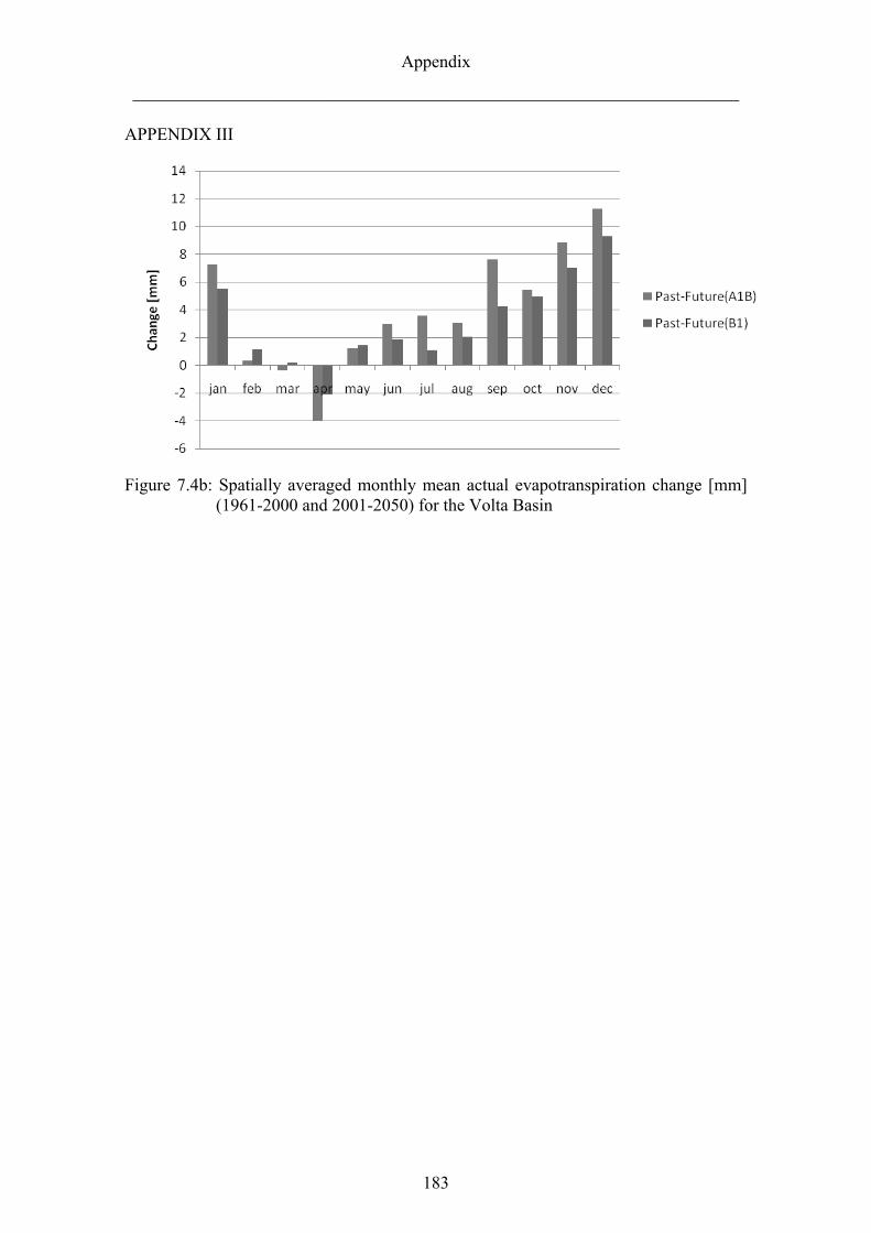
Appendix
_____________________________________________________________________
183
APPENDIX III
Figure 7.4b: Spatially averaged monthly mean actual evapotranspiration change [mm] (1961-2000 and 2001-2050) for the Volta Basin

Acknoledgements
_____________________________________________________________________
ACKNOWLEDGEMENTS
To GOD be the glory, great things He has done.
I would like to express my heartfelt gratitude to my supervisor Prof. Dr. Bernd
Diekkrueger, vice chair of the Department of Geography, University of Bonn, for his
continuous scientific guidance, support and supervision throughout the entire course of
this work. I have learned a lot from the fruitful discussions that we had, and have
greatly benefited from his experience. I am specifically grateful for his extraordinary
willingness to assist me whenever I needed help in every aspect of my work.
I would like also to thank my co-supervisor Prof. Dr. Paul Vlek, Director of the Center
for Development Research (ZEF), for giving me the opportunity to do my PhD at ZEF. I
very thankful to him for his useful comments and full support during my stay at ZEF.
I would like to thank the BMBF (Federal Ministry for Education and Research) for
providing me with the financial support for my PhD study in Bonn. The ZEF-GLOWA
Volta project deserves my special thanks for supporting my research expenses and also
for creating the best environment for my study. I would like to extend my thanks to the
entire staff members of ZEF, specifically to Dr. Günter Manske and Rosemarie Zabel. I
would also like to express my sincere appreciation to Mrs. Zabel for her extraordinary
assistance. I am really grateful for her readiness to help whenever I was in need. I would
like to extend my thanks to Dr. Constanze Leemhius and Dr. Charles Rodgers (previous
ZEF staff) for their constructive comments during this study and their valuable logistic
support most especially after my field work. This work would not have been possible
without the keen cooperation of the following people: Herwig Hölzel of the Department
of Geography of University of Bonn, Dr. Serge Shumilov of the Computer Science
Department of University of Bonn, Dr. Boubacar Barry of IWMI, Prof. Francis Allotey
of Ghana Atomic Energy, Prof Haruna Yakubu, Pro Vice Chancellor of University of
Cape Coast, Prof. Heiko Paeth of the GLOWA IMPETUS project and the
meteorological departments of Ghana and Burkina Faso. I would also like to extend my
deepest thanks to Daniel Ofori, Salisu Adams - of GLOWA Volta and now IWMI, not
only for their immense professional assistance but also for being good friends. My
drivers, Eli and Kwasi, deserve special thanks for assisting me during rough field work
and data gathering and collection.

Acknoledgements
_____________________________________________________________________
My special thanks go to my beloved parents who have given me their unconditional
love in my entire life, and have been the source of my strength all along. I would like
also to extend my gratitude to my dearest family Clara, Belinda, Martha, Gertrude,
Raymond Jr. and Borisa for providing me with their love and support throughout my
journey.