Embed Size (px)
Citation preview

Modelling Heavy Elements in a Dynamic
Chromosphere
Stefano PucciMaster’s thesis
Institute of Theoretical AstrophysicsUniversity of Oslo
December 2008


Preface
This thesis is the result from a collaboration between Iselin Bø and the un-dersigned, under the supervising of Øystein Lie-Svendsen. The collaborationconcerns in particular the implementation of the numerical model. This iswhy the chapters 2 and 3, which describe the physical problem and the workwith the code, are in common, i.e. are included in both the theses. However,the section 2.1.1, concerning the radiative ionisation, describes an approachthat differs from Bø’s thesis.
Once the main body of the code has been built, the two works havefollowed different paths.
The undersigned have studied a dynamic chromospheric layer with theaim to investigate the abundance variation in the fast solar wind. Bø hasinstead focused on the element fractionation resulting from a gravitationalsettling in a chromosphere without any net outflow of hydrogen.
I would like to thank my supervisor Øystein Lie-Svendsen for the innu-merable hours he dedicated to guide me through this project. Thanks alsoto Tara and Kosovare for proof reading this thesis, and special thanks to“nonne” Giovannella and Kirsten and “zia” Lilja. Finally great thanks toErika that reminded us of the importance of Astrophysics in our lives.
Oslo, December 2008
Stefano Pucci
i

ii

Contents
1 Introduction 1
1.1 Observations . . . . . . . . . . . . . . . . . . . . . . . . . . . . 21.2 Models . . . . . . . . . . . . . . . . . . . . . . . . . . . . . . . 71.3 The present work . . . . . . . . . . . . . . . . . . . . . . . . . 8
2 The model 9
2.1 Ionisation rates . . . . . . . . . . . . . . . . . . . . . . . . . . 112.1.1 Radiative Ionisation . . . . . . . . . . . . . . . . . . . 112.1.2 Collisional ionisation . . . . . . . . . . . . . . . . . . . 12
2.2 Recombination rates . . . . . . . . . . . . . . . . . . . . . . . 132.2.1 Radiative recombination for hydrogen . . . . . . . . . . 132.2.2 Recombination rates for the minor constituents . . . . 142.2.3 Dielectronic recombination rate for iron . . . . . . . . . 14
2.3 Charge transfer . . . . . . . . . . . . . . . . . . . . . . . . . . 142.4 Electric field . . . . . . . . . . . . . . . . . . . . . . . . . . . . 162.5 Collisions . . . . . . . . . . . . . . . . . . . . . . . . . . . . . 16
2.5.1 Neutral-neutral collisions . . . . . . . . . . . . . . . . . 172.5.2 Neutral-ion collisions . . . . . . . . . . . . . . . . . . . 172.5.3 Ion-ion collisions . . . . . . . . . . . . . . . . . . . . . 18
3 The numerical model 21
3.1 Double grid . . . . . . . . . . . . . . . . . . . . . . . . . . . . 213.2 Semi-implicit scheme . . . . . . . . . . . . . . . . . . . . . . . 223.3 Newton-Raphson method . . . . . . . . . . . . . . . . . . . . . 243.4 Boundary conditions . . . . . . . . . . . . . . . . . . . . . . . 26
4 The ionisation-diffusion model of Peter 29
5 The hydrogen background 33
5.1 Boundary conditions . . . . . . . . . . . . . . . . . . . . . . . 345.2 Results . . . . . . . . . . . . . . . . . . . . . . . . . . . . . . . 34
iii

iv CONTENTS
5.3 Discussion . . . . . . . . . . . . . . . . . . . . . . . . . . . . . 41
6 The minor constituents 45
6.1 Boundary conditions . . . . . . . . . . . . . . . . . . . . . . . 456.2 Oxygen . . . . . . . . . . . . . . . . . . . . . . . . . . . . . . 46
6.2.1 Results . . . . . . . . . . . . . . . . . . . . . . . . . . . 466.2.2 Discussion . . . . . . . . . . . . . . . . . . . . . . . . . 51
6.3 Low FIP elements . . . . . . . . . . . . . . . . . . . . . . . . . 536.3.1 Silicon . . . . . . . . . . . . . . . . . . . . . . . . . . . 536.3.2 Magnesium . . . . . . . . . . . . . . . . . . . . . . . . 556.3.3 Iron . . . . . . . . . . . . . . . . . . . . . . . . . . . . 606.3.4 Discussion . . . . . . . . . . . . . . . . . . . . . . . . . 62
6.4 Neon . . . . . . . . . . . . . . . . . . . . . . . . . . . . . . . . 636.4.1 Results . . . . . . . . . . . . . . . . . . . . . . . . . . . 636.4.2 Discussion . . . . . . . . . . . . . . . . . . . . . . . . . 68
7 Discussion 69
7.1 The background model . . . . . . . . . . . . . . . . . . . . . . 697.2 The minor constituents model . . . . . . . . . . . . . . . . . . 69
7.2.1 Searching for enrichment . . . . . . . . . . . . . . . . . 697.2.2 Additional results . . . . . . . . . . . . . . . . . . . . . 747.2.3 Gradual ionisation . . . . . . . . . . . . . . . . . . . . 79
8 Summary 81
Bibliography 82

Chapter 1
Introduction
Elemental abundance in the photosphere is believed to be homogeneous,and to represent the same abundance as the proto-nebula that formed thesolar system (Feldman and Laming, 2000). The high density and the strongconvection, in fact, leads to a well mixed photosphere.
However the composition of the upper atmosphere presents some signifi-cant variations from the photosphere. Furthermore different structures in thecorona and in solar wind show different abundances. Both in-situ measure-ments of solar wind and spectroscopic measurements of the coronal spectrumprovide evidence for a different level of abundance between the photosphereand the upper atmosphere.
In the upper atmosphere the elements with a low First Ionisation Po-tential (FIP ≤ 10eV) are enriched relative to high FIP elements and withrespect to the photospheric ratio.
This FIP effect can be quantified defining the relative and absolute frac-tionation for a generic element x:
(fabs)structurex =
(Aabs)structure
(Aabs)photosphere(1.1)
and
(frel)structurex =
(Arel)structure
(Arel)photosphere, (1.2)
where the absolute and relative abundances are defined as:
Aabs =Nx
NH
(1.3)
and
Arel =Nx
NO, (1.4)
1

2 CHAPTER 1. INTRODUCTION
FIP (eV) log Ax Nx/NH
H 13.6 12.00 1O 13.6 8.66 ± 0.05 1 (4.07 − 5.13) × 10−4
Ne 21.6 8.08 ± 0.06 (1.05 − 1.38) × 10−4
Mg 7.6 7.58 ± 0.05 (3.39 − 4.27) × 10−5
Si 8.1 7.55 ± 0.05 (3.16 − 3.98) × 10−5
Fe 7.9 7.50 ± 0.05 (2.82 − 3.55) × 10−5
Table 1.1: Photospheric abundances and first ionisation potentials for selectedelements (Grevesse and Sauval, 1998).
where NX is the total density of the considered element, NH and NO are thetotal hydrogen density and the total oxygen density.
This work will focus on the solar wind abundance variations.
1.1 Observations
The elemental abundances of the photosphere have been studied since 1929,when Russell (1929) analysed the spectrum of the solar photosphere anddetermined the abundances of 56 elements. Since then many measurementshave been done and the different elemental abundances are now believed tobe well known. The only exception is represented by oxygen, for which themeasured abundance has decreased by a factor of 0.46 from measurementsin 1989 to 2004 (Asplund et al., 2004).
The elemental abundances for the photosphere are shown in table 1.1.These values are given both in the standard logarithmic scale log Ax =12 + log10(Nx/NH) and as a simple density ratio, and are obtained by spec-troscopic measurements (Grevesse and Sauval, 1998).
To quantify the intensity of a line we can measure the equivalent width,which is related to the area between the line and the continuum intensity,in a plot of the intensity versus the wavelength. How the equivalent widthincreases with gas density is described by the curve of growth (Gray, 2005).Thus, by measuring the equivalent width and calculating the curve of growth,we can get an estimate for the density of the gas. The curve of growth is re-lated to many model parameters like temperature and levels population, butalso to atomic-physics quantities like transition probability. Hence obtaininga good estimate of elemental abundances from the line strength requires de-tailed models to describe both the solar atmosphere and the physics of the
1The oxygen abundance is taken from Asplund et al. (2004)

1.1. OBSERVATIONS 3
transitions.Another method to obtain an estimate of the photospheric abundances
consists of measuring the composition of a special kind of meteorite (CIcarbonaceous chondrites). These meteorites are believed to come from as-teroids that were not subject to the differentiation processes that affectedthe planet formation and thus are characterised by the same composition ofthe proto-nebula that formed the solar system. The chondrites abundancevalues confirm the spectroscopic values listed in table 1.1. This comparisonis obviously legitimated only for non-volatile elements, i.e. in our case formagnesium, silicon and iron.
While the photosphere is characterised by a homogeneous and constantcomposition, different structures of the upper atmosphere and solar windpresent important variations in the compositions. We will now focus on solarwind measurements.
The spacecraft Ulysses was the first satellite to complete a polar orbit (in-clination 80.22◦) around the sun. A review of the studies from Ulysses mea-surements of the solar wind composition can be found in von Steiger and Schwadron(2000). Measurements from the SWICS (Solar Wind Ion Composition Spec-trometer) instrument on board Ulysses confirm that the solar wind is mainlymade up of two fundamentally different components: fast wind and slowwind.
Fast solar wind is characterised by high velocities (≈ 750 km s−1 measuredat 1 AU) and a ratio between the charge states of a specific element (called thefreezing-in temperature) that reflects the coronal electron temperature abovecoronal hole regions (Feldman and Laming, 2000). There is in fact quite goodagreement on the source location of fast wind in the coronal holes. Coronalholes are regions where the coronal plasma is colder and characterised bya density lower than the typical values of temperature and density in thecorona. Normally coronal holes are located over the sun poles, but duringhigh activity periods coronal holes can extend to lower latitude regions andcausing fast solar wind to mix with slow wind in the ecliptic plane.
Slow solar wind is characterised by lower velocities (≈ 400 km s−1 mea-sured at 1 AU), and different from fast wind, no single electron tempera-ture can describe the spectra of elements (von Steiger and Schwadron, 2000).Slow solar wind seems to originate from quiet coronal regions but there isno full agreement upon its origin. Abundances comparison can suggest thecoronal loops as sources for slow wind, but this requires that these loops haveto open to release the plasma.
A third component of solar wind, associated with transient phenomena,appears during high activity periods and is called the Solar Energetic Particleevent.

4 CHAPTER 1. INTRODUCTION
Because of the much larger hydrogen abundance relative to the restof the solar abundant elements, it is easier to use another element (oxy-gen in most cases) for comparisons. In order to give an absolute meaningto these comparisons the hydrogen abundance relative to oxygen (or viceversa) is needed. With the SWICS instrument, the obtained hydrogen rel-ative abundance value (NH/NO) is: Arel = 1890 ± 600 in slow wind andArel = 1590 ± 500 in fast wind (von Steiger et al., 1995). With the photo-spheric value for the hydrogen relative abundance given by Asplund et al.(2004), Arel = 2190 ± 250, both slow and fast wind value are inside the un-certainty. Moreover the adopted value for the hydrogen relative abundancein the photosphere has been subject to numerous corrections in the last years(see also Grevesse and Sauval (1998)). Hence, there is no experimental evi-dence of an absolute fractionation for oxygen.
The SWICS instrument could measure and characterise the incomingions determining the energy per charge and the mass per charge. In thatway the instrument could perform comparable measurements of elementalabundances relative to wind velocity. A sample of these measurements, av-eraged over a 5-days period, is presented in Fig. 1.1. The green periodssample shows slow wind, measuring when Ulysses was passing at low lati-tudes (< 15◦), whereas the purple sample shows fast wind measuring over theSouth Pole. The low FIP element silicon presents a relative abundance thatis higher in slow wind than in fast wind. For the medium FIP element carbonthe picture is quite different with no significant variations between slow andfast wind. Another observation is that both of the relative abundances aremore variable in slow wind than in fast wind.
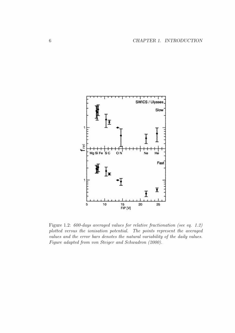
Fig. 1.2 shows relative fractionation values measured by SWICS, averagedover two periods for a total of ≈ 600 days, for both fast and slow wind. Inslow wind (upper panel) the fractionation for low FIP elements (magnesium,silicon, and iron), is a bit less than 3 and the medium FIP (sulphur andcarbon) are also enriched by a factor of ≈ 1.5. The high FIP element nitrogenand neon and the very high FIP helium are depleted relative to oxygen.
In fast wind the low FIP elements are still enriched but just by a factor of≈ 2 and the medium FIP elements are enhanced by approximately the samefactor as in slow wind. Nitrogen presents almost no depletion whereas neonand helium are still quite depleted.
Another difference between slow and fast wind, as already pointed, is thevariability of the values: the fractionation values in the fast wind are muchless variable than the respective values in slow wind.
These results changed the canonical picture of the FIP effect in solarwind. Previous measurements, made by satellites with low inclined orbits (seeTable 1 from von Steiger and Geiss (1989) for a review), gave an enrichment

1.1. OBSERVATIONS 5
Figure 1.1: 5-days averaged values for silicon relative abundance (lower panel)and carbon relative abundance (middle panel) from SWICS instrument incomparison to the solar wind speed of protons from SWOOPS (Solar WindsObservations Over the Poles of the Sun) instrument (upper panel). Figureadapted from von Steiger and Schwadron (2000).
6 CHAPTER 1. INTRODUCTION
Figure 1.2: 600-days averaged values for relative fractionation (see eq. 1.2)plotted versus the ionisation potential. The points represent the averagedvalues and the error bars denotes the natural variability of the daily values.Figure adapted from von Steiger and Schwadron (2000).
1.2. MODELS 7
of low FIP between 3.5 and 5 in slow wind, while almost no enrichment wasmeasured for the low FIP elements in the fast wind. Yet FIP elements wereobserved to present no depletion relative to oxygen. These measurementswere characterised by a plateau structure with the low FIP elements formingthe first plateau, the middle FIP elements being the transition part, and thehigh FIP elements forming a second plateau where they were not enrichedrelative to each others.
1.2 Models
Different theoretical models have been developed in order to explain the FIPeffect both in the upper solar atmosphere and in solar wind. Most of themodels locate the fractionation process in the chromosphere, where the firstionisation occurs.
The first kind of model neglects the role of the magnetic field in thefractionation, or use it only to guide the ions. In this model fractionationis driven by diffusion along field lines. Models of this kind are implementedby Marsch et al. (1995), Wang (1996) and Peter (1998). Peter’s model isexplained in detail in chapter 4. A common feature for these diffusion modelsis that an enrichment can be obtained if the minor constituent velocity at thebottom of the studied layer exceeds the velocity of the hydrogen background(see eq.4.10).
A second kind of model describes the magnetic field as the key elementin the fractionation process. At low enough densities, (such that neutral andionised atoms are not coupled) high FIP elements (that are still neutral)can move perpendicularly to the field lines, whereas this is not possible forlow FIP elements that at these chromospheric heights are already ionised.The fractionation thus derives from a difference in the drift velocities betweenhigh and low FIP elements. This velocity difference becomes significant whenthe collision frequency between ionised and neutral atoms can be neglectedrelative to the gyro frequency. Under this condition the neutral species (highFIP) can cross the field lines while the ionised species are forced to follow thefield. An example for this kind of models is given by Vauclair (1996) wherean ascending horizontal magnetic field lift the ionised elements, whereas theneutral cross the field lines because of gravity, leading to an enrichment oflow FIP element in the upper part of the atmosphere. Other models of thiskind are presented by von Steiger and Geiss (1989) and Henoux and Somov(1997).
8 CHAPTER 1. INTRODUCTION
1.3 The present work
There is still no wide agreement upon the processes behind the FIP effectand both more observation and more theoretical models are needed to obtaina clearer picture of the fractionation process.
In this work we will focus on the fractionation process in fast solar wind.Building a one dimensional numerical model of the chromosphere we will
try to understand the ionisation-separation process that is believed to bebehind fractionation. First we will implement a model describing the hy-drogen background in a chromospheric layer, with a flow corresponding tothe solar wind flux obtained by measurements. Three different supposed ge-ometry will give three different characteristic velocities for the model. Thenwe will build a similar model describing the interaction between some minorconstituents (oxygen, neon, magnesium, silicon and iron) and the hydrogenbackground in order to study how and if fractionation can take place, withdifferent background fluxes. The result will be compared with the work byPeter (1998) and Peter and Marsch (1998), discussing their ad-hoc chosenboundary conditions and parameters and how these influence the possibilityto obtain a FIP effect comparable with measurements.

Chapter 2
The model
We consider a slab of the solar atmosphere of a certain thickness and with acertain temperature profile. For simplicity we consider the atmosphere as aone dimensional system with plane parallel symmetry.
The atmosphere model consists of a pure hydrogen background (see sec-tion 5) and one of the trace elements (minor constituents) O, Ne, Mg, Si orFe at the time. Only neutrals and singly ionised particles are included, andthe hydrogen background is quasi neutral, i.e. the electron density is thesame as the proton density.
The physical quantities are governed by the mass conservation (masscontinuity equation) and the momentum equation (Newton’s second law).No energy equation is solved, but a linear temperature profile is given. Inthis way we avoid the problems related to the coupling between the radiativetransport equation and the hydrodynamic equations.
We consider a magnetic field with vertical magnetic flux lines and flow,in vertical direction only. Hence, since the contribution from the magneticfield is proportional to the vector product between the magnetic field and thevelocity, we do not need to include any magnetic field term in the momentumequation.
We model the following equations
∂ni
∂t+
∂
∂z(ni ui) = nj Pji − ni Pij (2.1)
∂(niui)
∂t+
∂
∂z(niuiui) = −
1
mi
∂
∂z(nikT ) + gni + njuj Pji − niuiPij
+niqi
miE +
∑
j 6=i
niνij(uj − ui) (2.2)
9
10 CHAPTER 2. THE MODEL
where the indexes i and j can take the values 1 or 2, representing neutral gasand ionised gas, respectively. ni is the number density and ui is the velocity ofthe species i. P12 is the ionisation rate and P21 the recombination rate, bothdiscussed in section 2.1. mi and qi are the mass and the electric charge of thespecies i, respectively. E is the electric field (see section 2.4) and νij is thecollision frequency between the species i and j. The collision frequencies aretreated in section 2.5. g is the gravitational acceleration, set to g = −270 ms−2, T is the temperature (constant in time) and k is Boltzmann’s constant.The derivatives in equation 2.1 and 2.2 are taken with respect to time t andheight z. All the variables are in SI-units, if nothing else is specified.
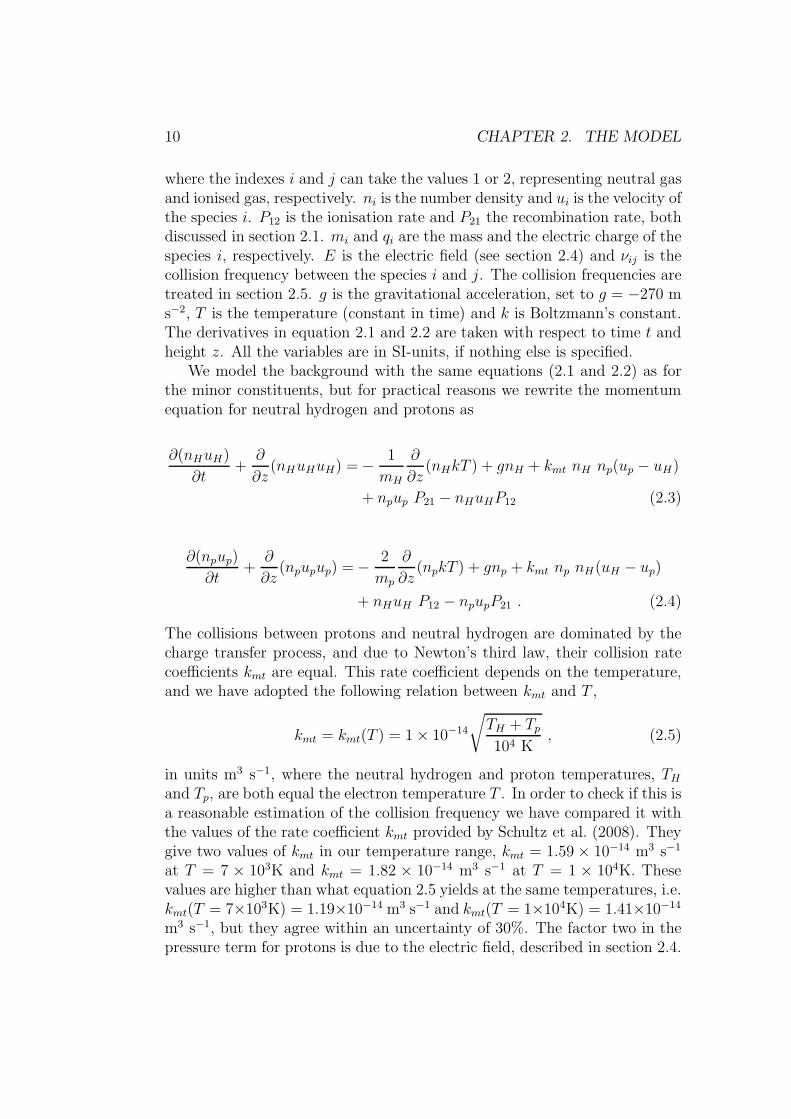
We model the background with the same equations (2.1 and 2.2) as forthe minor constituents, but for practical reasons we rewrite the momentumequation for neutral hydrogen and protons as
∂(nHuH)
∂t+
∂
∂z(nHuHuH) = −
1
mH
∂
∂z(nHkT ) + gnH + kmt nH np(up − uH)
+ npup P21 − nHuHP12 (2.3)
∂(npup)
∂t+
∂
∂z(npupup) = −
2
mp
∂
∂z(npkT ) + gnp + kmt np nH(uH − up)
+ nHuH P12 − npupP21 . (2.4)
The collisions between protons and neutral hydrogen are dominated by thecharge transfer process, and due to Newton’s third law, their collision ratecoefficients kmt are equal. This rate coefficient depends on the temperature,and we have adopted the following relation between kmt and T ,
kmt = kmt(T ) = 1 × 10⁻¹⁴
√
TH + Tp
104 K, (2.5)
in units m3 s−1, where the neutral hydrogen and proton temperatures, TH
and Tp, are both equal the electron temperature T . In order to check if this isa reasonable estimation of the collision frequency we have compared it withthe values of the rate coefficient kmt provided by Schultz et al. (2008). Theygive two values of kmt in our temperature range, kmt = 1.59 × 10⁻¹⁴ m3 s−1
at T = 7 × 10³K and kmt = 1.82 × 10⁻¹⁴ m3 s−1 at T = 1 × 10⁴K. Thesevalues are higher than what equation 2.5 yields at the same temperatures, i.e.kmt(T = 7×10³K) = 1.19×10⁻¹⁴ m3 s−1 and kmt(T = 1×10⁴K) = 1.41×10⁻¹⁴
m3 s−1, but they agree within an uncertainty of 30%. The factor two in thepressure term for protons is due to the electric field, described in section 2.4.

2.1. IONISATION RATES 11
2.1 Ionisation rates
The ionisation rate Pij can be written as the sum of the radiative ionisationRij and the collisional ionisation Cij ,
Pij = Rij + Cij . (2.6)
For the hydrogen background, the collisional ionisation rate is almost al-ways negligible. For oxygen we also take charge transfer with hydrogen intoaccount (see section 2.3). The collisional and radiative ionisation rates foroxygen are negligible.
2.1.1 Radiative Ionisation
Hydrogen For the radiative ionisation we follow the approach of Peter and Marsch(1998). In that model the ionising radiation is assumed to come from above.In other words the photons that have the right energy to ionise hydrogen areassumed to come from the upper layers of the solar atmosphere. Supposinga constant photon flux at the top of our layer, the ionising radiation flux andthe photoionisation rate R12 vary with depth in the atmosphere. Assuming aphotoionisation cross section σH that is constant for the relevant wavelengthband we can write:
d
dsR12 = −σHR12nH , (2.7)
where s = ztop − z is the depth, z the height, ztop the height of the layer’supper boundary and nH is the neutral hydrogen density. The photoioni-sation cross section for hydrogen can be estimated as σH = 5.5 × 10⁻²² m2
(Peter and Marsch, 1998) (Vernazza et al., 1981). Solving equation 2.7, witha change of variable from s to z we get:
R12(z) = R12 (ztop) exp
(
−σH
∫ ztop
z
nH(z′)dz′)
. (2.8)
If the neutral hydrogen density is known the rate can be estimated by nu-merical integration.
By supposing an initial value for R12(z) we can integrate the fluid equa-tions until we obtain a steady state. With nH we can calculate a new valuefor R12 from equation 2.8. We continue the iteration until R12 changes byless than 3% from one iteration to the next.
Minor constituents For the radiative ionisation of the minor constituentswe follow the approach of Peter (1998). As for hydrogen the ionising radi-ation is assumed to come from above, that gives a decaying ionisation rate.

12 CHAPTER 2. THE MODEL
Rni[s−1]
O 1.62 × 10⁻²
Ne 1.24 × 10⁻²
Si 9.23 × 10⁻¹
Mg 1.28Fe 1.099
Table 2.1: Ionisation rates.
However the minor constituents are characterised by a low abundance. Thisgives a negligible absorption of the ionising radiation. The ionisation ratecan thus be considered constant throughout the slab.
The photoionisation rates for zero optical depth are given in table 2.1 andare taken from von Steiger and Geiss (1989) and Peter (1998).
2.1.2 Collisional ionisation
There are several different ionisation mechanisms due to collisions. We onlyconsider direct ionisation in this work. Direct ionisation happens when anatom collides with an electron producing two electrons and a singly ionisedatom. The direct ionisation rates for the elements H, O, Ne, Mg and Si aretaken from Arnaud and Rothenflug (1985), while the direct ionisation ratefor iron is taken from Arnaud and Raymond (1992). The rate coefficient fordirect ionisation can be written
cDI(T ) = 6.69 · 10−13
( e
kT
)3/2 exp(−x)
xF (x) , (2.9)
in units of m3 s−1, where
x =eI
kT(2.10)
F (x) =A (1 − x f1(x)) + B (1 + x − x(2 + x)f1(x))
+ C f1(x) + D x f2(x) (2.11)
f1(x) =ex
∫ ∞
1
dt
te−tx (2.12)
f2(x) =ex
∫ ∞
1
dt
te−tx ln(t) . (2.13)
I is the first ionisation potential in units V, e is the elementary charge andA, B, C and D are fitting coefficients given in table 2.2. The integral f1(x)

2.2. RECOMBINATION RATES 13
is evaluated using the Hastings polynomial approximation
x f1(x) = x ex
∫ ∞
1
dt
te−tx =
x4 + a1x3 + a2x
2 + a3x + a4
x4 + b1x3 + b2x2 + b3x + b4
+ ǫ(x) , (2.14)
(Abramowitz and Stegun, 1964), where |ǫ(x)| < 2 × 10⁻³ and
a1 = 8.573328740 b1 = 9.573322345 (2.15)
a2 = 18.05901697 b2 = 25.63295615 (2.16)
a3 = 8.634760893 b3 = 21.09965308 (2.17)
a4 = 0.267773734 b4 = 3.958496923 . (2.18)
f2(x) is evaluated following Hummer (1983), and the final ionisation rate C12
defined in chapter 2 is given by
C12 = cDI np , (2.19)
in units s−1.
2.2 Recombination rates
The recombination rate P21 of the minor constituents can be written as thesum of the radiative recombination R21 and the dielectronic recombinationD21. The radiative recombination is a form of spontaneous emission. Thedielectronic recombination is a process where an unbound electron binds tothe recombining ion giving its energy to the atom by exciting one of its otherelectrons. The excited atom deexcitates by emitting a photon. For hydrogenwe obviously only have radiative recombination.
2.2.1 Radiative recombination for hydrogen
The radiative recombination rate coefficient for hydrogen is given by
αr(T ) = 5.197 × 10⁻²⁰ λ1/2(
0.4288 + 0.5 ln(λ) + 0.469 λ−1/3)
, (2.20)
(Arnaud and Rothenflug, 1985), in units m3 s−1, where λ = 157890/T andT is given in K. In order to get the rate Rij measured in s−1, as defined inchapter 2, αr(T ) has to be multiplied by the electron number density, whichin our model is the same as the proton number density,
P21 = R21 = αr np. (2.21)

14 CHAPTER 2. THE MODEL
2.2.2 Recombination rates for the minor constituents
The equation for the radiative recombination rate coefficient in units m3 s−1
(Shull and van Steenberg, 1982) is the same for all the minor constituents,
αr(T ) = Arad
(
T
104K
)Xrad
. (2.22)
The fitting coefficients, Arad and Xrad, are given in table 2.3. Also the dielec-tronic recombination rate coefficient, in units m3 s−1 (Shull and van Steenberg,1982), is the same for O, Ne, Mg and Si,
αd(T ) = Adi T− 3
2 exp
(
−T0
T
) (
1 + Bdi exp
(
−T1
T
))
. (2.23)
The fitting coefficients Adi, Bdi, T0 and T1 are given in table 2.3. As for hydro-gen, these rate coefficients have to be multiplied with the electron (proton)density in order to get the recombination rate P21 in units of s−1,
P21 = R21 + D21 = (αr + αd) np. (2.24)
2.2.3 Dielectronic recombination rate for iron
The equation for the dielectronic recombination rate for iron is given by
αd(T ) = T− 3
2
∑
j
cj exp
(
−Ej e
kT
)
, (2.25)
in units m3 s−1 (Arnaud and Raymond, 1992). Ej and cj are given by
E1 = 5.12 eV c1 = 2.2 × 10⁻¹⁰ m3 s−1 K3/2 (2.26)
E2 = 12.9 eV c2 = 1.0 × 10⁻¹⁰ m3 s−1 K3/2 . (2.27)
2.3 Charge transfer
The charge transfer ionisation and charge transfer recombination are, in afirst approximation, the predominant transition processes for oxygen. Inthe charge transfer ionisation an electron jumps from a neutral oxygen to aproton resulting in a ionised oxygen and neutral hydrogen atom. Vice versa,in charge transfer recombination, an ionised oxygen and a neutral hydrogenmeet to form neutral oxygen and a proton. Treating this process as a normal

2.3. CHARGE TRANSFER 15
Element I A B C DO 13.6 9.5 -17.5 12.5 -19.5Ne 21.6 40.0 -42.0 18.0 -56.0Mg 7.6 18.0 -1.0 0.6 -4.0Si 8.1 74.5 -49.4 1.3 -54.6Fe 7.9 31.9 -15.0 0.32 -28.1
Table 2.2: Fitting coefficients for the direct ionisation rates.
Arad (m3 s−1) Xrad Adi (m3 s−1 K3/2) Bdi T0 (K) T1 (K)O 3.10(-19) 6.78(-1) 1.11(-9) 9.25(-2) 1.75(5) 1.45(5)Ne 2.20(-19) 7.59(-1) 9.77(-10) 7.30(-2) 3.11(5) 2.06(5)Mg 1.40(-19) 8.55(-1) 4.49(-10) 2.10(-2) 5.01(4) 2.81(4)Si 5.90(-19) 6.01(-1) 1.10(-9) 0.0 7.7(4) 0.0Fe 1.42(-19) 8.91(-1) - - - -
Table 2.3: Fitting coefficients for the recombination rates. 3.10(−19) means3.10 × 10−19.
transition between neutral and ionised oxygen the transition rates are givenby
P12 = np CION (2.28)
P21 = nH CREC (2.29)
in units s−1, where np and nH is the proton and the neutral hydrogen numberdensity, respectively. The rate coefficients CION and CREC are given by
CION =0.91 × 10⁻¹⁵ exp
(
−19.6 × 10⁻³ V
kTe
)(
1 − 0.93 exp
(
−T
103K
))
(2.30)
CREC =10−15
(
1 − 0.66 exp
(
−9.3T
104K
))
, (2.31)
in units m3 s−1 (Arnaud and Rothenflug, 1985).

16 CHAPTER 2. THE MODEL
2.4 Electric field
To obtain a simple expression for the electric field we write the momentumequation for the electrons,
∂(neue)
∂t+
∂
∂z(neueue) = −
1
me
∂
∂z(nekT ) + gne −
nee
meE , (2.32)
where me is the electron mass, ne is the electron number density, ue is thevelocity of the electrons. Since the electron mass me is much smaller thanevery other variable, we can neglect all the terms that are not divided by me,and equation 2.32 becomes
−∂
∂z(nekT ) = ne e E . (2.33)
We have assumed that the sun’s atmosphere is quasi neutral, and hencene = np. Substituting this in equation 2.33 we obtain
−∂
∂z(npkT ) = np e E , (2.34)
which yields the following expression for the electric field,
E = −1
e np
∂
∂z(npkT ) . (2.35)
2.5 Collisions
The collision processes describe how the minor constituents interact withthe hydrogen background. In this section we will treat three different colli-sion processes. Neutral-neutral collisions (collisions between neutral minorconstituents and neutral hydrogen), neutral-ion collisions (both collisions be-tween neutral minor constituents and protons, and collisions between neutralhydrogen and ionised minor constituents), and finally the very importantcollisions between ionised particles (protons and ionised minor constituents).Collisions between two minor constituents are neglected.
Proton-ion collisions are the absolutely strongest ones. Their rate co-efficients are at least two (often three) orders of magnitude stronger thanthe rate coefficients for neutral-ion and neutral-neutral collisions. Neutral-neutral and neutral-ion collisions have rate coefficients of the same order ofmagnitude.

2.5. COLLISIONS 17
Element rnH(10−10m)Oxygen 2.26Neon 1.75Silicon 2.91
Magnesium 3.09Iron 3.09
Table 2.4: Atomic radius for the rigid sphere approximation, taken fromMarsch et al. (1995).
2.5.1 Neutral-neutral collisions
When describing the collisions between neutral particles we use the so calledrigid sphere approximation. The collision frequency for neutral-neutral colli-sions (Banks and Kockarts, 1973) (Schunk, 1977) is given by
ν12 =4
3
m2
m1 + m2
n2 σ0 v12 , (2.36)
in units s−1, where m1 and m2 are the masses of the colliding particles, v12
is the relative velocity, n2 is the number density of the neutral hydrogengas, and σ0 = πr2
nH is the collision cross section. The values of rnH forthe different minor constituents (Marsch et al., 1995) are given in table 2.4.Assuming thermal and dynamic equilibrium, the distribution of the velocitiesis given by the Maxwell distribution and the average relative speed betweenthe particles is
v12 =
(
8 k
π
T
µ
)1
2
, (2.37)
where the reduced mass µ is given by
µ =m1 m2
m1 + m2
. (2.38)
Equation 2.36 and 2.37 yields the following expression for the collision fre-quency,
ν12 =4
3
m2
m1 + m2
n2 σ0
(
8 k
π
T
µ
)1
2
. (2.39)
2.5.2 Neutral-ion collisions
In a neutral-ion collision the most important interaction is represented byan induced dipole attraction. The average collision rate (Schunk, 1977), in

18 CHAPTER 2. THE MODEL
Element αHydrogen 0.74Oxygen 0.88
Iron 9.3Neon 0.44Silicon 6.0
Magnesium 11.8
Table 2.5: Neutral gas atomic polarizability. [α] = 10−40 C2 s2 kg−1
units s−1, is given by
ν12 =4
3
m2
m1 + m2
n2 v12 QD. (2.40)
n2 is now or the neutral or the ionised hydrogen number density, and QD isthe average momentum transfer cross section for collisions between ions andneutral particles, given by
QD = 0.260( α
kT
)1
2 e
ǫ0
, (2.41)
where α is the neutral gas atomic polarizability and ǫ0 is the permittivityof vacuum. The polarizabilities α for the different elements (Marsch et al.,1995) are given in table 2.5. The average relative speed is given by the sameformula as for collisions between neutral particles (see equation 2.37), andwith the expression for the cross section in equation 2.41, equation 2.40 canbe written as
ν12 = 0.553m2
m1 + m2
n2
(
α
µ
)1
2 e
ǫ0
. (2.42)
2.5.3 Ion-ion collisions
Collisions between charged particles are described by the so called Coulombinteraction. The collision frequency for such collisions (Schunk, 1977), inunits s−1, is given by
ν12 =1
3 ǫ20
n2 m2
m1 + m2
(
2πkT
µ12
)− 3
2 e21 e2
2
µ212
ln Λ , (2.43)
where the electric charge e1 and e2 of the two particles are, in our case, bothequal the elementary charge e. This is because we only treat singly ionised

2.5. COLLISIONS 19
ions. The Coulomb logarithm, ln Λ, is given by
Λ = 24π ne L3D , (2.44)
where LD is the Debye length, that for a pure hydrogen plasma is given by
LD =
(
4π
kT
e2
4πǫ0
(ne + np)
)− 1
2
. (2.45)
Since we study a quasi neutral atmosphere, i.e. ne = np, equation 2.45 maybe written as
LD =
√
kTǫ0
2e2np
. (2.46)
Finally we obtain the following expression for the Coulomb logarithm,
ln Λ = ln
(
24πnp
e3
(
kTǫ0
2np
)3
2
)
. (2.47)

20 CHAPTER 2. THE MODEL
Chapter 3
The numerical model
3.1 Double grid
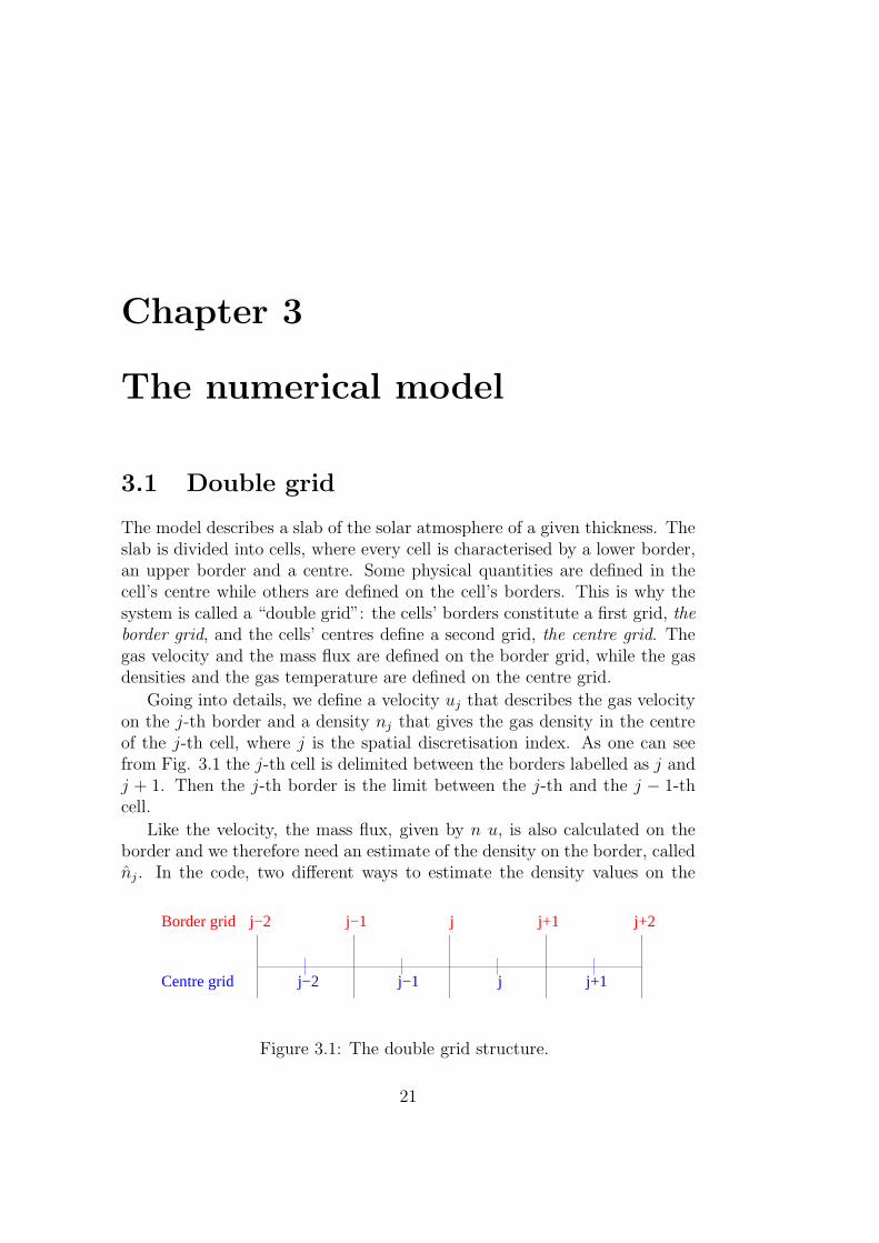
The model describes a slab of the solar atmosphere of a given thickness. Theslab is divided into cells, where every cell is characterised by a lower border,an upper border and a centre. Some physical quantities are defined in thecell’s centre while others are defined on the cell’s borders. This is why thesystem is called a “double grid”: the cells’ borders constitute a first grid, theborder grid, and the cells’ centres define a second grid, the centre grid. Thegas velocity and the mass flux are defined on the border grid, while the gasdensities and the gas temperature are defined on the centre grid.
Going into details, we define a velocity uj that describes the gas velocityon the j-th border and a density nj that gives the gas density in the centreof the j-th cell, where j is the spatial discretisation index. As one can seefrom Fig. 3.1 the j-th cell is delimited between the borders labelled as j andj + 1. Then the j-th border is the limit between the j-th and the j − 1-thcell.
Like the velocity, the mass flux, given by n u, is also calculated on theborder and we therefore need an estimate of the density on the border, callednj . In the code, two different ways to estimate the density values on the
j+1j j+2j−1j−2
j−2 j−1 j j+1
Border grid
Centre grid
Figure 3.1: The double grid structure.
21

22 CHAPTER 3. THE NUMERICAL MODEL
borders have been used. The first one is an easy two points average,
nj =1
2(nj−1 + nj), (3.1)
and the second one is a more elaborated average using a second order upwinddifferencing scheme to estimate an advective flux. The two points averageis used in all terms of equation 2.2, except the first term on the right handside (pressure gradient term), which has no need for any value of nj , andthe second term on the left hand side (advection term), where the upwindscheme is used. The latter is also used in the second term of the left handside of equation 2.1.
In the same way, we can define the averaged velocity of the cell centre,
uj =1
2(uj + uj+1), (3.2)
but this time only the two points average has been used.
3.2 Semi-implicit scheme
The aim of the code is to integrate the continuity and the momentum equa-tions (equation 2.1 and 2.2) in time. The scheme used to solve these equationsis a semi-implicit scheme, which means that it is a mix of an explicit and animplicit scheme.
In the explicit part every unknown variable is a function of known vari-ables only. To exemplify we consider the quantity q(p, r), which is a func-tion of the quantities p and r. In an explicit scheme at a certain time stepi + 1, the quantity q is only a function of p and r at previous time steps,qi+1 = qi+1(pi, ri, pi−1, ...). The explicit scheme for the left hand side of thecontinuity equation is given by
ni+1j − ni
j
∆t+
(
nij+1 ui
j+1 − nij ui
j
)
∆z. (3.3)
Thus, the explicit scheme provides an easy way to determine numericallythe evolution of the physical quantities when the values at the previous timestep are known. Unfortunately, explicit methods are characterised by unsta-ble solutions. These can be studied introducing the Courant-Friedrichs-Lewystability criterion (Press et al., 1992), which sets a lower limit for the ratiobetween spatial increment ∆z and time step ∆t.
The code is used to find both time dependent and steady state solutions,which requires big time steps. It is therefore preferable to avoid any upper

3.2. SEMI-IMPLICIT SCHEME 23
limit for the time step ∆t. In order to avoid this, we need to use an implicitscheme.
In implicit schemes, the quantity qi+1 is coupled with all the other quan-tities at the same time step, qi+1 = q(pi+1, ri+1, pi, ri, ...). It is therefore nolonger possible to calculate explicitly every quantity one by one. Hence, thewhole system of coupled equations needs to be solved for each time step ti.The implicit scheme for the left hand side of the continuity equation becomes
ni+1j − ni
j
∆t+
(
ni+1j+1 ui+1
j+1 − ni+1j ui+1
j
)
∆z. (3.4)
Since all the quantities are coupled in the implicit scheme, there is noupper limit for time step ∆t. In our code implicit and explicit parts aremixed, i.e. the variables in the advective term of the continuity equation(2.1) and the momentum equation (2.2) are defined as
uj = β ui+1j + (1 − β) ui
j (3.5)
and¯nj = β ni+1
j + (1 − β) nij, (3.6)
where β determines how implicit the code is. β = 0 gives a fully explicitcode, β = 1 gives a fully implicit code, and any number between 0 and 1makes the code semi-implicit.
By defining the cell volume ∆V = A∆z, where A is the unit surface,equation 3.3 can be written as
∆V(
ni+1j − ni
j
)
+ A∆t(
¯nj+1 uj+1 − ¯nj uj
)
= 0. (3.7)
The discretisation of the right hand side of the continuity equation (equa-tion 2.1) proceeds similarly, with the only note that we choose to write theionisation term as a fully implicit - and not semi-implicit - term.
Also the discretisation of the momentum equation follows the same steps,and the explicit expression for the left hand side of equation 2.2 is,
ni+1j ui+1
j − niju
ij
∆t+
(
nij+1u
ij+1 + ni
juij
)
uij −
(
niju
ij + ni
j−1uij−1
)
uij−1
∆z. (3.8)
A combination of equation 3.8 and the corresponding implicit scheme givesthe semi-implicit expression
∆V(
ni+1j ui+1
j − niju
ij
)
+ A∆t(
¯nj+1uj+1 + ¯nj uj
)
¯uj
−(
¯njuj + ¯nj−1uj−1
)
¯uj−1 , (3.9)

24 CHAPTER 3. THE NUMERICAL MODEL
where we have defined
¯uj = β ui+1j + (1 − β) ui
j . (3.10)
Without going into details, we will describe how the different terms onthe right hand side of the momentum equation (2.2) can be implementedin a discretised scheme, by specifying if the implicit or semi-implicit form isused. The pressure gradient term contains semi-implicit centre-grid valuesof the density, defined similarly to equation 3.6. The electric field term isequal to the pressure gradient term in the hydrogen background, which meansthat it contains semi-implicit centre-grid values of the (proton) density. Inthe code for the minor constituents the electric field depends on the fullyimplicit minor constituent density value at the cell borders, and on the time-independent proton pressure also evaluated at the cell borders. The gravityterm depends on the semi-implicit border-grid values of the density. Theionisation, the charge transfer and the collision terms are calculated fromfully implicit border-grid values of the density and the velocity.
3.3 Newton-Raphson method
As we have seen in section 3.2, a semi-implicit scheme leads to a system ofcoupled nonlinear equations that we want to solve with respect to ni+1 andui+1 for every time step i. In order to do this, the Newton-Raphson methodis applied (Press et al., 1992). As a first step, we define a vector Ej thatcontains all the discretised system equations, both for the continuity and forthe momentum equation. These equations have a component for every cellj.
The solution for the i + 1 time step yields the value ni+1 and ui+1 forwhich
Ej(ni+1
k , ui+1
k , ni+1
k−1, . . .) = Ej(x
i+1
k , . . .) = 0, (3.11)
where xik is a vector of components ni
k, uik, and k is a second space index.
We write xi+1
k as the sum of the previous value xik and a correction ∆xi
k,
xi+1
k = xik + ∆xi
k, (3.12)
where ∆xik is the unknown variable. If the time step is small enough, we
assume that also the corrections are small,
|∆xik|
xik
≪ 1. (3.13)

3.3. NEWTON-RAPHSON METHOD 25
With this assumption it is possible to linearise the solution, neglecting thehigher order terms in |∆x|
x, e.g.,
xi+1
k · xi+1
k ≈ xik · x
ik + 2xi
k∆xik + higher orders. (3.14)
Let us assume that we do not know the real solutions xi+1
k , but only theirestimate xt
k, called test solution. Then the vector E is no longer zero, butquantifies the error from the estimate. The aim of the Newton-Raphsonmethod is to find the right correction that nullifies the error, or at leastmakes it negligible. The steps of the Newton-Raphson method are given by
Ej(xtk) 6= 0, (3.15)
Ej(xtk + ∆xk) = 0. (3.16)
Assuming again that the correction is small, |∆xk|xt
k
≪ 1, we can rewrite Ej as
a Taylor series
Ej(xtk + ∆xk) ≈ Ej(x
tk) +
∑
k
∂Ej
∂xk
∣
∣
∣xk=xtk
∆xk = 0. (3.17)
By defining a new operator Wjk as
Wjk = −∂Ej
∂xk, (3.18)
we can rewrite equation 3.17 as
Ej(xtk + ∆xk) ≈ Ej(x
tk) −
∑
i
Wjk(xtk)∆xk = 0, (3.19)
or in matrix formW · ∆x = E(xt). (3.20)
If we invert the matrix W, we get
∆x = W−1E(xt), (3.21)
that allows us to calculate a new value of x,
xt′ = xt + ∆x. (3.22)
The partial derivatives that constitute the matrix element Wjk are dif-ferent from zero only when j − 2 ≤ k ≤ j + 2, because of the second order

26 CHAPTER 3. THE NUMERICAL MODEL
upwind scheme used in the advective term. This results in a pentadiagonalmatrix, with big simplifications concerning the matrix inversion.
The Newton-Raphson method gives exact result when the system is madeup of linear equations. This is not the case here, because in the Taylorexpansion we have neglected all the higher order terms including the secondorder. However, if the test solution is not too far from the real solution,i.e. |∆x|
x≪ 1, hopefully the new solution obtained with the Newton-Raphson
method can bring us closer to the right solution. If this is the case, we cansolve the system with an iterative procedure, otherwise, if the new solutionis not converging, it is necessary to repeat the whole process with a smallertime step ∆t.
3.4 Boundary conditions
In this section we will describe the role of the boundary conditions, and howthey are implemented. The physical values of the boundary conditions arenot the same for the background and the minor constituents, and also varybetween the different background models. They are therefore given for eachspecific case in later sections.
The boundary conditions are very important because they describe thephysical system outside the grid and constitute the way to communicate allthe necessary external conditions to the modelled layer. For example it isthrough the boundary conditions that we simulate the presence of the atmo-sphere below the lower boundary, avoiding in this way the whole atmosphereto fall in a gravitational collapse.
The boundary conditions supply the values for the border density n (seesection 3.1) and the border velocity u on the left border of the first cell andon the last cell’s right border.
It is important to differentiate the fixed and the floating boundary con-ditions. While a fixed boundary forces the boundary to have a determinedvalue, the floating condition allows the boundary to just follow the same be-haviour as the nearby grid points. A typical example of a floating boundaryequation is the flux conservation, where the particle flux is conserved fromthe first grid point to the second.
Specifying a fixed density value simulates a rigid wall at the beginningor end of the grid, and can often cause reflection problems. In order to giveinformation about the physical system without building a reflective wall weuse the method of characteristics described by Korevaar and van Leer (1988).
The main idea is to build a boundary condition that has a non-reflectivebehaviour but is still carrying information from the system outside the grid.

3.4. BOUNDARY CONDITIONS 27
This is achieved by a set of equations that permits the boundary to oscillatearound a fixed value, in order for the perturbations to pass through it.
Lower boundary This method considers a undisturbed hydrogen gas atthe lower boundary (where z = z0) which has fixed values for the densityand velocity, no and uo, respectively. The true boundary value nl and ul arecalculated by a sort of interpolation between the undisturbed values no anduo and the densities and velocities at the first and the second grid pointn1,u1, n2 and u2. The boundary condition for the density is then given by
nl =1
kT0
exp
(
γ(al + u0 − u1) + c0 log(n0kT0) + c1 log(n1kT1)
c0 + c1
)
(3.23)
where co =√
kT0
mHis the sound speed of a pure hydrogen gas at temperature
T0, and mH is the hydrogen mass. γ is the heat capacity ratio, and theparameter al is given by
al =z1 − z0
z2 − z1
[
c2
γlog
(
n1T1
n2T2
)
− (u1 − u2)
]
. (3.24)
where ci, Ti, and zi are the sound speed, the temperature and the height forthe first (i = 1) and the second (i = 2) grid point. The boundary conditionfor the velocity is given by
ul = u0 −c0
γlog
(
nl
n0
)
. (3.25)
Upper boundary The conditions for the upper boundary follow the sameprinciples as for the lower boundary. The undisturbed values n0, u0 andnTOP , uTOP are specified in the different cases presented later.

28 CHAPTER 3. THE NUMERICAL MODEL

Chapter 4
The ionisation-diffusion model
of Peter
We are now describing the model by Peter (1998).Since we have such a different behaviour between high and low FIP ele-
ments (see Fig. 1.2), the basic separation process is believed to happen inthe chromosphere, at altitudes where elements can be found in both ionisedand neutral state.
The fractionation is caused by two distinct processes: ionisation and dif-fusion. Elements with low FIP are characterised by a small ionisation timeand they therefore couple early with the main flux of solar wind, because ofthe very effective Coulomb collisions with protons. Yet high FIP elementsneed longer time to ionise and are later coupled with hydrogen in solar wind.Thus low FIP elements are easier transported out of the chromosphere.
The other important process is diffusion. At the bottom of the ionisationlayer different velocities for different elements are possible (no coupling) andthese different velocities cause different abundances.
There is also a third effect that influences the fractionation, that is thevelocity dependence. If the main stream of hydrogen has a high velocity, thetime needed to pass through the ionisation layer is smaller and the fractiona-tion process is less effective. If instead the wind speed is lower, the ionisation-diffusion process has more time and higher fractionation is reached.
Starting from the fluid equations, it is possible to obtain a simple for-mula that describes fractionation. We write the continuity equation (eq.2.1)and the momentum equation (eq.2.2) for the neutral state of a generic minorconstituent x, while we assume a constant background of hydrogen. The fol-lowing assumptions and approximations are used: steady state (all the timederivatives are zero), subsonic velocity (the advective term of the momen-tum equation can be neglected), thin slab (negligible gravity and constant
29
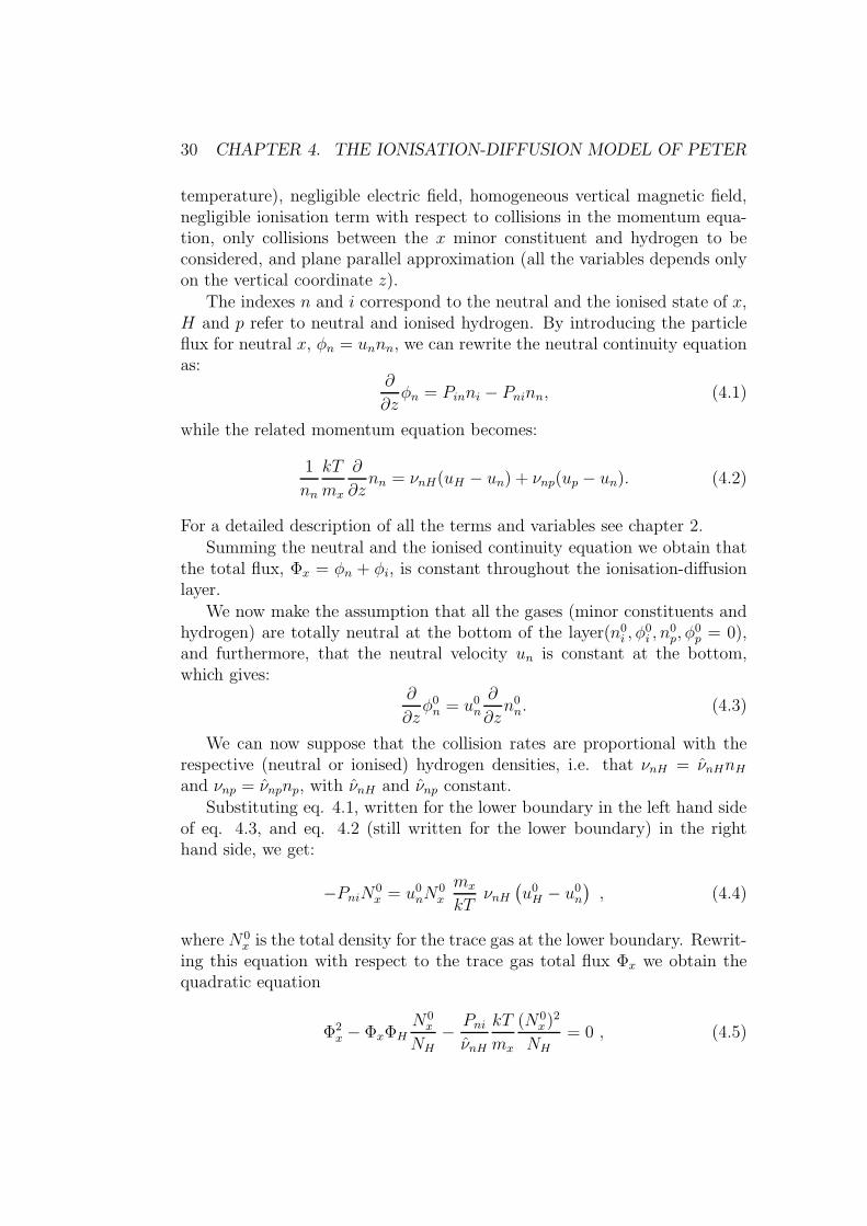
30 CHAPTER 4. THE IONISATION-DIFFUSION MODEL OF PETER
temperature), negligible electric field, homogeneous vertical magnetic field,negligible ionisation term with respect to collisions in the momentum equa-tion, only collisions between the x minor constituent and hydrogen to beconsidered, and plane parallel approximation (all the variables depends onlyon the vertical coordinate z).
The indexes n and i correspond to the neutral and the ionised state of x,H and p refer to neutral and ionised hydrogen. By introducing the particleflux for neutral x, φn = unnn, we can rewrite the neutral continuity equationas:
∂
∂zφn = Pinni − Pninn, (4.1)
while the related momentum equation becomes:
1
nn
kT
mx
∂
∂znn = νnH(uH − un) + νnp(up − un). (4.2)
For a detailed description of all the terms and variables see chapter 2.Summing the neutral and the ionised continuity equation we obtain that
the total flux, Φx = φn + φi, is constant throughout the ionisation-diffusionlayer.
We now make the assumption that all the gases (minor constituents andhydrogen) are totally neutral at the bottom of the layer(n0
i , φ0i , n
0p, φ
0p = 0),
and furthermore, that the neutral velocity un is constant at the bottom,which gives:
∂
∂zφ0
n = u0n
∂
∂zn0
n. (4.3)
We can now suppose that the collision rates are proportional with therespective (neutral or ionised) hydrogen densities, i.e. that νnH = νnHnH
and νnp = νnpnp, with νnH and νnp constant.Substituting eq. 4.1, written for the lower boundary in the left hand side
of eq. 4.3, and eq. 4.2 (still written for the lower boundary) in the righthand side, we get:
−PniN0x = u0
nN0x
mx
kTνnH
(
u0H − u0
n
)
, (4.4)
where N0x is the total density for the trace gas at the lower boundary. Rewrit-
ing this equation with respect to the trace gas total flux Φx we obtain thequadratic equation
Φ2x − ΦxΦH
N0x
NH−
Pni
νnH
kT
mx
(N0x)2
NH= 0 , (4.5)

31
which gives the following solutions:
Φx =ΦH
N0x
NH±
√
Φ2H
(
N0x
NH
)2
+ 4(ωxN0x)2
2; (4.6)
where capital letters stay for total densities and total fluxes and where ωx,called the diffusion velocity, is defined by:
ω2x =
Pni
νnHNH
kT
mx. (4.7)
By defining the average velocity U = Φ/N , eq. 4.6 can be rewritten as:
Ux
UH
= 1 ±
√
1 + 4
(
ωx
UH
)2
. (4.8)
With an upstream only the plus sign leads to a physical solution. From eq.4.8 it results that all the minor constituents have a velocity at the bottomhigher than the main stream velocity.
This ratio between average velocities is closely related to the fractiona-tion. Supposing that the key processes for fractionation take place in thisionisation-diffusion layer, the absolute fractionation (see eq. 1.1) can berewritten as:
(fabs)x =( Nx
NH)top
( Nx
NH)bottom
. (4.9)
If we now assume that at top the velocities are all coupled, Ux = UH , andconsider that the total fluxes are constant, the ratio Nx/NH at the top isequal to the ratio Φx/ΦH , that gives:
(fabs)x =U0
x
U0H
. (4.10)
Also the relative fractionation can be written from eq. 4.8:
(frel)x =Ux
Uo
=1 +
√
1 + 4(
ωx
UH
)2
1 +
√
1 + 4(
ωO
UH
)2. (4.11)
Thus the relative fractionation is determined only by the diffusion velocityω and by the main stream velocity UH . Eq. 4.11 describes how the different

32 CHAPTER 4. THE IONISATION-DIFFUSION MODEL OF PETER
processes (ionisation and diffusion) influence the fractionation: with a largerionisation rate we get a higher fractionation, while with a higher collision rate,i.e. higher coupling between the minor constituent and hydrogen, a lowerdiffusion velocity and a lower fractionation are obtained. From this equationwe also get a description of the velocity dependence: a lower velocity of thehydrogen background gives an higher FIP effect, with the limit situation ofnegligible hydrogen velocity and a fractionation given by the ratio betweenthe diffusion velocities.

Chapter 5
The hydrogen background
In order to study the fractionation for minor constituents, a hydrogen back-ground model is needed. Since the fractionation is believed to be related tothe ionisation processes, it is important to focus on the altitude where thisionisation takes place. Hence, both the slab thickness and the slab locationare chosen with respect to this criterion.
In this work we study the fractionation related to fast solar wind. Thismeans that the background model describes a dynamic atmosphere with agiven net hydrogen particle flux. The observed fast solar wind flux at 1 AU isΦ1AU ≈ 2×10¹² m−2 s−1. Assuming flux conservation from the sun’s surfaceto 1 AU radius, we get
f r21AU Φ1AU = r2
S ΦS, (5.1)
that results in
ΦS = f Φ1AUr21AU
r2S
, (5.2)
where the parameter f represents a geometry factor that describes differentareal expansions. Using the values r1AU = 1.496 × 10¹¹ m and rSUN =6.96 × 10⁸ m, we get ΦSUN = f × 9.24 × 10¹⁶ m−2 s−1.
We choose three values for the geometry factor f = 1, f = 20 andf = 100. f = 1 represents the radial expansion geometry. f = 20 is the mostprobable value following the work of Byhring et al. (2008) (model F1), basedon measured Doppler shift of minor ion spectra lines from the transitionregion and the corona. f = 100 is the geometry factor used by Peter (1998).These three models are be called “L”,“M” and “H” respectively.
The slab thickness is 1000 km and the chosen linear temperature profileis shown in Fig. 5.1
33

34 CHAPTER 5. THE HYDROGEN BACKGROUND
Temperature
0 5•105 1•106
height [m]
0
5.0•103
1.0•104
1.5•104
Tem
pera
ture
[K]
Figure 5.1: The chosen linear temperature profile.
5.1 Boundary conditions
In order to repeat the calculation by Peter (1998), we build a model similarto the background described by Peter and Marsch (1998), using almost thesame boundary conditions.
At the lower boundary, the neutral hydrogen density is assumed to be8 × 1016 m−3. The gas streaming up through the lower boundary is set tobe ca 2% ionised. This condition does not constrain the ionisation degree tohave a fixed value on the first grid point.
The photoionisation rate at the top of the layer is set to be RHp = 0.014s−1 (Peter and Marsch, 1998). The condition of a solar wind stream throughour atmosphere is imposed via the proton velocity at the upper boundary.The flux takes three different values for the three different cases L, M andH. The neutral hydrogen and ionised velocities at the top are forced to beequal.
In table 5.1 the values for all the physical parameters are shown.
5.2 Results
We run the code from an initial condition, where the gas is uniformly 1%ionised and the neutral hydrogen profile follows the hydrostatic equilibrium,until we have reached the steady state (104 s).

5.2. RESULTS 35
Lower boundary: Total density N0 = 8 × 10¹⁶ m−3
Ionisation degree 0.018Upper boundary: Ionisation rate 0.014 s−1
Velocity uH = up
Total flux ΦH = 9 × 10¹⁶, 2 × 10¹⁸, 9 × 10¹⁸ m−2 s−1
Table 5.1: The boundary conditions used for the background model. Only thefixed boundary conditions are reported.
Total density
0 5•105 1•106
height [m]
1015
1016
1017
NH[m
-3]
HML
Figure 5.2: The total hydrogen density profile.

36 CHAPTER 5. THE HYDROGEN BACKGROUND
Neutral density
0 5•105 1•106
height [m]
1014
1015
1016
1017
n H [m
-3]
HML
Figure 5.3: The neutral hydrogen density profile.
The sum of the neutral and ionised hydrogen density profiles is shown forthe three wind fluxes H, M and L in Fig. 5.2. The density decreases slightlywith increasing flux, but the differences between the densities in the threecases are very small.
The neutral and ionised density profiles are shown in Fig. 5.3 and Fig.5.4, respectively. For neutral hydrogen the L and M profiles are almostequal while the H profile has a bit higher density. The proton densities donot follow a monotone profile, but reach a top near z = 2 × 10⁵ m. Thedifferences between the H, M and L profiles are bigger than in the neutralcase, and the higher flux the lower density.
The ionisation rates for the H, L and M cases are shown in Fig. 5.5. Allthe profiles have a monotone behaviour, with a rate increasing more rapidlyin the lower part of the slab. The figure shows the sum of the radiative andcollisional ionisation rates, but the latter constitutes less than 5% of the totalrate.
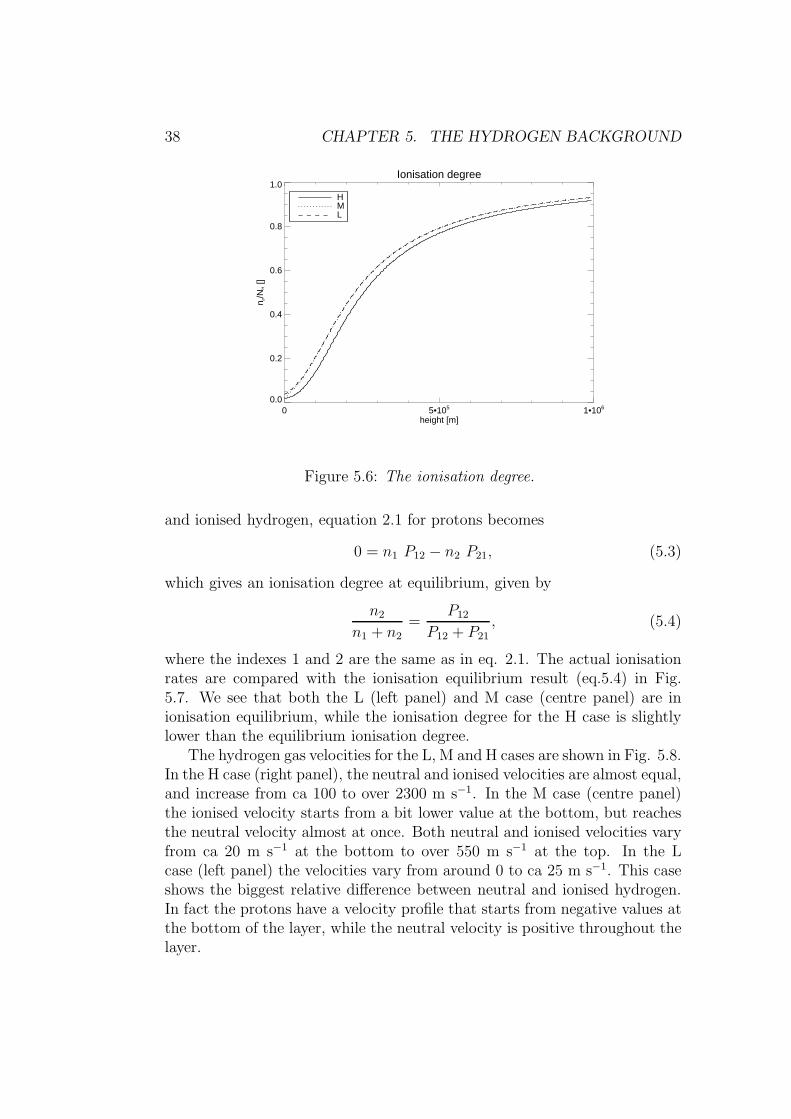
Fig. 5.6 shows the ionisation degree for the three flux cases. These profilesfollow the ionisation rates shown in Fig. 5.5 and justify our choice for theslab thickness, since we are interested in studying the ionisation area. Whilethe L and M cases have the same ionisation degree, the H case differs fromthe other two with an almost constant gap.
If one supposes a static situation with zero particle flux for both neutral

5.2. RESULTS 37
Ionised density
0 5•105 1•106
height [m]
1015
1016
1017
n P [m
-3]
HML
Figure 5.4: The proton density profile.
Ionisation rates
0 5•105 1•106
height [m]
0.000
0.005
0.010
0.015
Rat
es [s
-1]
HML
Figure 5.5: The ionisation rates.
38 CHAPTER 5. THE HYDROGEN BACKGROUND
Ionisation degree
0 5•105 1•106
height [m]
0.0
0.2
0.4
0.6
0.8
1.0
n p/N
H []
HML
Figure 5.6: The ionisation degree.
and ionised hydrogen, equation 2.1 for protons becomes
0 = n1 P12 − n2 P21, (5.3)
which gives an ionisation degree at equilibrium, given by
n2
n1 + n2
=P12
P12 + P21
, (5.4)
where the indexes 1 and 2 are the same as in eq. 2.1. The actual ionisationrates are compared with the ionisation equilibrium result (eq.5.4) in Fig.5.7. We see that both the L (left panel) and M case (centre panel) are inionisation equilibrium, while the ionisation degree for the H case is slightlylower than the equilibrium ionisation degree.
The hydrogen gas velocities for the L, M and H cases are shown in Fig. 5.8.In the H case (right panel), the neutral and ionised velocities are almost equal,and increase from ca 100 to over 2300 m s−1. In the M case (centre panel)the ionised velocity starts from a bit lower value at the bottom, but reachesthe neutral velocity almost at once. Both neutral and ionised velocities varyfrom ca 20 m s−1 at the bottom to over 550 m s−1 at the top. In the Lcase (left panel) the velocities vary from around 0 to ca 25 m s−1. This caseshows the biggest relative difference between neutral and ionised hydrogen.In fact the protons have a velocity profile that starts from negative values atthe bottom of the layer, while the neutral velocity is positive throughout thelayer.

5.2. RESULTS 39
H Ionisation equilibrium
0 5•105 1•106
height [m]
0.0
0.2
0.4
0.6
0.8
1.0
n p/N
H []
M Ionisation equilibrium
0 5•105 1•106
height [m]
0.0
0.2
0.4
0.6
0.8
1.0
n p/N
H []
L ionisation equilibrium
0 5•105 1•106
height [m]
0.0
0.2
0.4
0.6
0.8
1.0
n p/N
H []
ion. equi.ion. deg.
Figure 5.7: The ionisation degree plotted together with the ionisation degreeat equilibrium.
H velocity
0 5•105 1•106
height [m]
0
500
1000
1500
2000
2500
u [m
s-1]
NeutralIonised
M velocity
0 5•105 1•106
height [m]
0
100
200
300
400
500
600
u [m
s-1]
L velocity
0 5•105 1•106
height [m]
-5
0
5
10
15
20
25
30
u [m
s-1]
Figure 5.8: The neutral and ionised hydrogen velocity profiles.
40 CHAPTER 5. THE HYDROGEN BACKGROUND
H-flux
0 5•105 1•106
height [m]
0
2•1018
4•1018
6•1018
8•1018
u n
[m-2 s
-1]
M-flux
0 5•105 1•106
height [m]
0
5.0•1017
1.0•1018
1.5•1018
2.0•1018
u n
[m-2 s
-1]
L-flux
0 5•105 1•106
height [m]
-2•1016
0
2•1016
4•1016
6•1016
8•1016
1•1017
u n
[m-2 s
-1]
IonisedNeutral
Figure 5.9: The neutral and ionised hydrogen flux profiles.
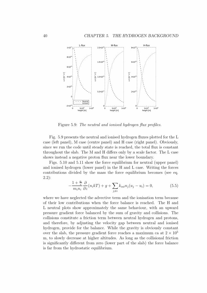
Fig. 5.9 presents the neutral and ionised hydrogen fluxes plotted for the Lcase (left panel), M case (centre panel) and H case (right panel). Obviously,since we run the code until steady state is reached, the total flux is constantthroughout the slab. The M and H differs only by a scale factor. The L caseshows instead a negative proton flux near the lower boundary.
Figs. 5.10 and 5.11 show the force equilibrium for neutral (upper panel)and ionised hydrogen (lower panel) in the H and L case. Writing the forcescontributions divided by the mass the force equilibrium becomes (see eq.2.2):
−1 + qi
e
mini
∂
∂z(nikT ) + g +
∑
j 6=i
kmtnj(uj − ui) = 0, (5.5)
where we have neglected the advective term and the ionisation term becauseof their low contributions when the force balance is reached. The H andL neutral plots show approximately the same behaviour, with an upwardpressure gradient force balanced by the sum of gravity and collisions. Thecollisions constitute a friction term between neutral hydrogen and protons,and therefore, by adjusting the velocity gap between neutral and ionisedhydrogen, provide for the balance. While the gravity is obviously constantover the slab, the pressure gradient force reaches a maximum ca at 2 × 10⁵
m, to slowly decrease at higher altitudes. As long as the collisional frictionis significantly different from zero (lower part of the slab) the force balanceis far from the hydrostatic equilibrium.

5.3. DISCUSSION 41
H-Neutral force equilibrium
0 5•105 1•106
height [m]
-400-200
0
200
400
600800
For
ce p
er m
ass
unit
[m s
-2]
H-Ionised force equilibrium
0 5•105 1•106
height [m]
-3000-2000
-1000
0
1000
20003000
For
ce p
er m
ass
unit
[m s
-2]
collisionspressure gradient + electric field
gravity
Figure 5.10: The force equilibrium for neutral and ionised hydrogen, H case.
The picture is quite different for protons (lower panel). Here the pressuregradient, which has to be added to the electric field, provides a downwardforce which is balanced by a positive collisional friction. In the lower partof the slab, gravity is, by comparison, almost negligible. In the upper partthe pressure gradient force gives a positive contribution, balancing gravityin hydrostatic equilibrium. The pressure gradient in the L case increasesmonotonously, while in the H case it decreases to a minimum at ca 5 × 10⁴
m and then it increases.
5.3 Discussion
Since the flux is subsonic, the density profile remains almost unchanged forthe different flux cases.
The ionisation degree for all the models follows the same profile as thephotoionisation rate, and the ionisation degree is close to ionisation equilib-rium. However, the departure from the ionisation degree at equilibrium getsbigger with higher fluxes, while the ionisation degree decreases.
This fact is easily understandable by using the ionisation length concept.Let’s say that a neutral gas needs a given time τION to get ionised up tothe ionisation equilibrium, where this ionisation time is given by the ionisa-tion degree at equilibrium divided by the ionisation rates. If the neutral gas

42 CHAPTER 5. THE HYDROGEN BACKGROUND
L-Neutral force equilibrium
0 5•105 1•106
height [m]
-400-200
0
200
400
600800
For
ce p
er m
ass
unit
[m s
-2]
L-Ionised force equilibrium
0 5•105 1•106
height [m]
-3000-2000
-1000
0
1000
20003000
For
ce p
er m
ass
unit
[m s
-2]
collisionspressure gradient + electric field
gravity
Figure 5.11: The force equilibrium for neutral and ionised hydrogen,L case.
streams through the layer with a velocity U , it will cover a distance LION , be-fore it reaches the ionisation equilibrium, which is given by: LION = U τION .So the higher wind flux we have, the bigger the ionisation length becomes,and a bigger gap between ionisation degree and equilibrium can be expected.For example, by comparing the ionisation degree (dashed line in the rightpanel of Fig. 5.7) with the ionisation degree at equilibrium (dotted line) inthe H case, we get that the former is delayed with respect to the latter bya distance ∆z ≈ 5 × 10⁴ m. This value is comparable with the calculatedionisation length at the first grid point, LION ≈ 1×10⁵ m. In the L case thiseffect is not visible at all. The negative and low positive proton velocitiesnear the lower boundary force the recently ionised hydrogen to stop. So, evenif the ionisation process takes a long time, the protons can accumulate untilthey reach the ionisation equilibrium; in other words the ionisation lengthapproximation makes no sense if the proton velocities are too different fromthe neutral hydrogen velocities. This effect plays an even more importantrole for the minor constituents. Furthermore, the fact that in the L case theionisation equilibrium is reached already at the first grid point while in the Hcase the ionisation process is delayed, explains the large difference in protondensity near the lower boundary between the H and L case (see Fig. 5.4).
The relative difference between neutral and ionised hydrogen velocitychanges for L, M and H, but by studying the absolute difference one can seethat this difference does not vary too much between the three cases.
The neutral hydrogen velocity is bigger than the proton velocity because

5.3. DISCUSSION 43
the ionisation process leads to a density profile with a positive pressure gra-dient force, higher than what gravity manages to balance. This upward forceincreases the neutral hydrogen velocity until the force is balanced by colli-sional friction. For protons we have a similar dynamic: the ionisation processleads, in the lower part of the layer, to an increasing density profile and asubsequent negative pressure gradient force. In this case too, the collisionalfriction balances this downward pressure gradient. In the upper part of thelayer, hydrogen is ionised to a high percent and the pressure gradient forcefor protons becomes positive.
This relationship can also be studied analytically by supposing force bal-ance between gravity, pressure (and electric field) and collisions. Subtractingeq.5.5 (written for protons) from the respective hydrogen equation and ne-glecting temperature gradient with respect to density gradient we obtain:
−kT
mH
(
d
dzlog nH − 2
d
dzlog nP
)
+ kmt(up − uH)NH = 0, (5.6)
where the index H refers to neutral hydrogen and p to protons. NH = nH+np
is the total hydrogen density. We finally obtain that
up − uH =k
kmtmH
T
NH
d
dz
(
lognH
n2p
)
, (5.7)
which clearly shows how velocity differences depend only on density profilesand on temperature profile. Eq. 5.7 states also that a non-homogeneousionisation degree leads to a difference between hydrogen and proton velocity.By a comparison between the analytical and numerical model it results thateq. 5.7 is a very good approximation and permits a correct understanding ofthe force equilibrium in the hydrogen background.
The obtained difference between neutral and ionised hydrogen velocityis therefore coupled with the density profiles and finally with the ionisationdegree. Since the L, M and H cases have a very similar ionisation degree, alsothe absolute differences between ionised and neutral velocities are similar.This result also tells us that a lower boundary condition that forces theneutral and ionised velocity to be equal should not be adopted together witha varying ionisation degree.

44 CHAPTER 5. THE HYDROGEN BACKGROUND

Chapter 6
The minor constituents
We now solve the equation 2.1 and 2.2 for the minor constituents oxygen,neon, silicon, magnesium and iron, until steady state is reached. This willrequire different running times for the code since every model has its char-acteristic evolution time.
Each element is studied with three different backgrounds L, M, and H,which correspond to three different choices of the geometry factor f .
For some minor constituents the ionisation-recombination dynamic isdriven by radiative processes (see section 2.1.1 and αr in section 2.2.2) whilefor other elements also the collisional processes are important (see section2.1.2 and αd in 2.2.2). For oxygen charge exchange is the dominant channelfor the ionisation process.
We run the code from an initial condition where the minority gas is 0.1%ionised with an absolute abundance Aabs = 5 × 10⁻⁴ uniform over the slab.This gives a start distribution that follows the same behaviour as the back-ground hydrogen profile.
6.1 Boundary conditions
No condition constrains the velocities for the minor constituents, i.e. theyare determined by the force balance at lower and upper boundary.
At the lower boundary, in order to simplify comparisons, Aabs = 5× 10⁻⁴
for all the minor constituents.
If the velocities near the lower boundary are positive the ionisation degreeof the gas streaming through the lower boundary is set to 0.01, otherwise thedensity values on lower boundary are calculated via an upwind differencingscheme.
45

46 CHAPTER 6. THE MINOR CONSTITUENTS
Oxygen absolute abundance
0 5•105 1•106
Height [m]
10-12
10-10
10-8
10-6
10-4
10-2
AA
BS []
LMH
Figure 6.1: The oxygen absolute abundance.
6.2 Oxygen
Oxygen has a peculiar behaviour because it is coupled to hydrogen via thevery effective charge transfer channel.
Both the radiative and collisional ionisation and recombination can beneglected with an error not bigger than 1%.
We run the code for 104 s for the H case, 105 s for the M, and 5 × 10⁶ sfor the L case, in order to reach the steady state.
6.2.1 Results
Fig. 6.1 shows the absolute abundances for the H, L and M cases. The H andM cases show a very slowly decreasing absolute abundance with altitude. Inthe H case the abundance decreases from the boundary/initial value 5×10⁻⁴
to 4 × 10⁻⁴ in the lower part of the slab and then it flattens out almostcompletely. The same behaviour is shown in the M case where Aabs decreasesto ca 2 × 10⁻⁴. The L case presents a radically different picture where theabsolute abundance is reduced by a factor of 107. This abundance decreasesexponentially up to z = 3 × 10⁵ m but flattens out throughout the rest ofthe grid.
Since the initial condition has a homogeneous absolute abundance, thetime needed to obtain the steady state increases radically from the H to theL case.

6.2. OXYGEN 47
Oxygen ionisation degree
0 5•105 1•106
Height [m]
0.0
0.2
0.4
0.6
0.8
1.0
n OII /
NO []
HML
Figure 6.2: The oxygen ionisation degree.
The oxygen ionisation degree is presented in Fig. 6.2, showing an ionisa-tion degree very similar to hydrogen (see Fig. 5.6). The L and M cases havethe same ionisation degree profile, while the H case presents a slightly lowerionisation degree.
The velocities for neutral and ionised oxygen, plotted together with theproton velocities, are shown in Fig. 6.3. In the H case (right panel), the pro-ton and the ionised oxygen velocities are coincident, and the neutral velocitiesare also very similar to them. In the M case (centre panel), the differencebetween the ionised and neutral oxygen velocities becomes more appreciable,while the ionised oxygen and protons velocities are still coupled. The L case(left panel) shows a quite different picture where the neutral oxygen veloci-ties decrease from zero at the lower boundary to quite high negative values.The ionised velocities rise from a negative value at the lower boundary andfollow the proton velocities for the rest of the grid.
The fractionation process for a minor constituent X can be studied (seeeq.4.10) by introducing the average velocity UX :
UX =nnun + niui
NX, (6.1)
where, the indexes n and i refer to the neutral and ionised specie. Fig. 6.4shows the ratio between the oxygen and hydrogen average velocities. For allthe three flux cases the oxygen velocity at lower boundary is lower than thehydrogen velocity, and then it increases. The oxygen and hydrogen velocities

48 CHAPTER 6. THE MINOR CONSTITUENTS
H- velocity
0 5•105 1•106
Height [m]
0
500
1000
1500
2000
2500
u [m
s-1]
NeutralIonisedProton
M- velocity
0 5•105 1•106
Height [m]
0
100
200
300
400
500
600
u [m
s-1]
L- velocity
0 5•105 1•106
Height [m]
-60
-40
-20
0
20
40
u [m
s-1]
Figure 6.3: The neutral and ionised oxygen velocity profiles.
at the upper border are coupled for the H and M cases, while the L case showsan oxygen velocity that remains relatively much lower than the hydrogen one.
By studying the velocity difference between ionised and neutral oxygen(left panel of Fig. 6.5) we see that this difference remains almost unchangedby varying the flux. The right panel of Fig. 6.5 shows the difference betweenthe ionised oxygen and proton velocities, giving a measurement of how muchthese are coupled. The departure of the ionised oxygen velocities from pro-tons is, except at lower altitudes, very similar in the three cases.
Fig. 6.6 shows the neutral and ionised oxygen flux for the three cases.The net flux is ≈ 3 × 10¹⁵ m−2 s−1 for the H case, ≈ 4 × 10¹⁴ m−2 s−1 forM but only ≈ 5 × 10⁶ m−2 s−1 in the L case. In the L case both the neutraland ionised flux fall to zero already at z = 105 m, and below this altitudethe neutral flux is positive and the ionised is negative. By dividing the netoxygen flux with the net hydrogen flux we get the relative net flux for oxygen.In the H case the relative net flux is ≈ 4×10⁻⁴, for M ≈ 2×10⁻⁴ and for theL case the flux is ≈ 6× 10⁻¹¹. The net relative flux gives approximately thesame value as the absolute abundance at the top of the slab (see Fig. 6.1)and it is therefore a good way to study how much of the minor constituentis dragged out by hydrogen.

6.2. OXYGEN 49
Oxygen averaged velocity
0 5•105 1•106
Height [m]
0.0
0.2
0.4
0.6
0.8
1.0U
O /
UH []
LMH
Figure 6.4: The ratio between the oxygen and hydrogen average velocities.
0 5•105 1•106
Height [m]
-20
0
20
40
60
80
u OII-u
OI [
m s
-1]
0 5•105 1•106
Height [m]
-10
-8
-6
-4
-2
0
u OI-u
p [m
s-1]
LMH
Figure 6.5: The velocity difference between ionised and neutral oxygen (leftpanel).The velocity difference between ionised oxygen and protons(right panel)
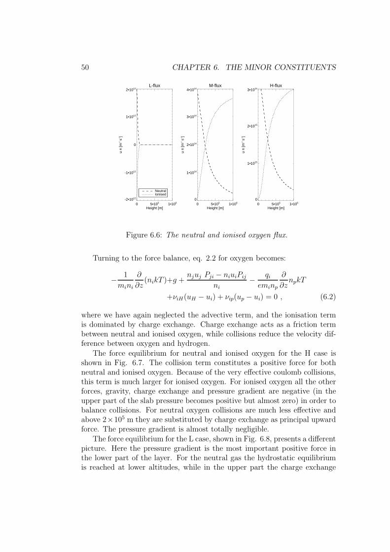
50 CHAPTER 6. THE MINOR CONSTITUENTS
H-flux
0 5•105 1•106
Height [m]
0
1•1015
2•1015
3•1015
u n
[m-2 s
-1]
M-flux
0 5•105 1•106
Height [m]
0
1•1014
2•1014
3•1014
4•1014
u n
[m-2 s
-1]
L-flux
0 5•105 1•106
Height [m]
-2•1012
-1•1012
0
1•1012
2•1012
u n
[m-2 s
-1]
IonisedNeutral
Figure 6.6: The neutral and ionised oxygen flux.
Turning to the force balance, eq. 2.2 for oxygen becomes:
−1
mini
∂
∂z(nikT )+g +
njuj Pji − niuiPij
ni−
qi
eminp
∂
∂znpkT
+νiH(uH − ui) + νip(up − ui) = 0 , (6.2)
where we have again neglected the advective term, and the ionisation termis dominated by charge exchange. Charge exchange acts as a friction termbetween neutral and ionised oxygen, while collisions reduce the velocity dif-ference between oxygen and hydrogen.
The force equilibrium for neutral and ionised oxygen for the H case isshown in Fig. 6.7. The collision term constitutes a positive force for bothneutral and ionised oxygen. Because of the very effective coulomb collisions,this term is much larger for ionised oxygen. For ionised oxygen all the otherforces, gravity, charge exchange and pressure gradient are negative (in theupper part of the slab pressure becomes positive but almost zero) in order tobalance collisions. For neutral oxygen collisions are much less effective andabove 2×10⁵ m they are substituted by charge exchange as principal upwardforce. The pressure gradient is almost totally negligible.
The force equilibrium for the L case, shown in Fig. 6.8, presents a differentpicture. Here the pressure gradient is the most important positive force inthe lower part of the layer. For the neutral gas the hydrostatic equilibriumis reached at lower altitudes, while in the upper part the charge exchange

6.2. OXYGEN 51
H-Neutral force equilibrium
0 5•105 1•106
Height [m]
-400
-200
0
200
400
For
ce p
er m
ass
unit
[m s
-2]
H-Ionised force equilibrium
0 5•105 1•106
Height [m]
-1000
-500
0
500
1000
1500
For
ce p
er m
ass
unit
[m s
-2]
gravitypressure gradient + electric field
charge exchangecollisions
Figure 6.7: The oxygen force equilibrium in the H case.
friction balances gravity. In the lower part of the slab, the L case shows,relative to the H case, a much lower collisional friction. This friction becomescomparable with the pressure gradient and the charge exchange.
6.2.2 Discussion
The oxygen ionisation degree is almost the same as hydrogen. This factcan be easily understood by studying the charge exchange process. SinceCion and Crec from eq.2.28 differ by less than 10%, the ionisation degree atequilibrium can be written as:
ni
ni + nn=
np
nHCrec
Cion+ np
≈np
nH + np. (6.3)
In all the flux cases oxygen is depleted with respect to hydrogen. In theH and M cases, however, the absolute abundance is almost constant and theoxygen is dragged up by hydrogen. The absolute abundance of oxygen in theL cases falls by a factor of 107.
The ionised oxygen velocity is almost totally coupled with the protonvelocity and the gap between them does not vary too much between the H,M and L cases.
From the force equilibrium for ionised oxygen in both the L and the Hcase we see that on the upper part of the slab the collisional friction is the

52 CHAPTER 6. THE MINOR CONSTITUENTS
L-Neutral force equilibrium
0 5•105 1•106
Height [m]
-400
-200
0
200
400
For
ce p
er m
ass
unit
[m s
-2]
L-Ionised force equilibrium
0 5•105 1•106
Height [m]
-1000
-500
0
500
1000
For
ce p
er m
ass
unit
[m s
-2]
gravitypressure gradient + electric fieldcharge exchangecollisions
Figure 6.8: The oxygen force equilibrium in the L case.
only force that balances gravity. The difference between the ionised oxygenand proton velocities is thus given by:
ui − up =g
ν2p
, (6.4)
where ν2p is the collisional rate for Coulomb collisions. Eq. 6.4 explains whythis velocity difference has the same profile for the three flux cases exceptat lower altitudes, where the pressure and the charge exchange are no longernegligible.
In order to obtain an absolute enrichment the element average velocity(eq. 6.1) at the left boundary must be larger than the hydrogen average ve-locity (see eq. 4.10). Neither the ionised nor the neutral oxygen velocities arelarger than the hydrogen velocities and no enrichment is therefore obtained.
One of the largest difference for neutral oxygen between the H and Lcase is that collisions with hydrogen are significant for the H case at loweraltitudes, while they are negligible for the L case, where the pressure gradi-ent balances gravity. In order to understand the reasons of this differencewe study the time development for the neutral oxygen force equilibrium atlower altitudes. Initially all the cases, L, M and H, reach the same free fallequilibrium where collisions with neutral hydrogen balance gravity, giving
uH − un ≈ −g
νnH. (6.5)

6.3. LOW FIP ELEMENTS 53
This value is nearly constant for the three flux cases and gives a velocitydifference of about 20 m s−1. While in the H case the hydrogen velocity atthe lower boundary is ≈ 100 m s−1, in the L case uH is just ≈ 1 m s−1 . Inorder to obtain a collision force able to balance gravity, the neutral oxygenvelocity must be negative and with falling oxygen a pressure gradient can bebuild.
The hydrostatic equilibrium in the lower part of the slab for the L caseleads to a strongly decreasing abundance.
6.3 Low FIP elements
6.3.1 Silicon
In the ionisation process the radiative ionisation rate is dominant by a factorof 103 over the collisional rate at the bottom, while at the top of the layerthey become of the same order of magnitude. In the recombination processthe dielectronic recombination rate is a factor of 10 smaller than the radiativerecombination rate at the bottom, but dominates by a factor of 7 over theradiative at the top.
We run the code for 5× 10⁶ s, 2× 10⁴ s and 1× 10⁴ s in the L, M and Hcase respectively in order to reach a steady state.
The incoming gas has an ionisation degree of 1% while the gas at thefirst grid point is 99% ionised. Some dynamic (see chapter 7) caused bythis huge difference lead to a lower boundary density value that does notbehave like a fixed boundary. Thus, in order to compare the abundances fordifferent elements and for different flux cases, it has been necessary to makea normalisation of the density values.
Fig. 6.9 shows the absolute abundance for silicon for the L case (leftpanel) and for the M and H cases (right panel). The absolute abundancedecreases with height for all the cases. The decreasing factor for the H andM cases is not larger than one third of the lower boundary value, whereasfor the L case the abundance decreases by a factor of 1010.
In Fig. 6.10 the silicon relative abundance is shown. In the H and M casesthe relative abundance shows an increasing behaviour that leads to a relativeenrichment with respect to oxygen. The increasing factor is larger for the Mcase. The L case, on the other hand, shows a relative abundance decreasingby a factor of 106, reaching a minimum at z = 105 m, and increasing againby a factor of 103.
The ionisation degree of silicon, presented in Fig. 6.11, is almost totallyconstant for the three flux cases and describes a fully ionised gas. Even in

54 CHAPTER 6. THE MINOR CONSTITUENTS
L
0 5•105 1•106
Height [m]
10-14
10-12
10-10
10-8
10-6
10-4
10-2
AA
BS []
H and M
0 5•105 1•106
Height [m]
0.0000
0.0001
0.0002
0.0003
0.0004
0.0005
AA
BS []
LMH
Figure 6.9: The silicon absolute abundance.
L
0 5•105 1•106
Height [m]
10-8
10-6
10-4
10-2
100
AR
EL [
]
H and M
0 5•105 1•106
Height [m]
0.0
0.5
1.0
1.5
AR
EL [
]
LMH
Figure 6.10: The silicon relative abundance.

6.3. LOW FIP ELEMENTS 55
Silicon ionisation degree
0 5•105 1•106
Height [m]
0.90
0.95
1.00
1.05
1.10
n SiII /
NS
i []
HML
Figure 6.11: The silicon ionisation degree.
the H case it is not possible to see any ionisation length effect (see section5.3). That is because the ionisation rate is too large and consequently theionisation length too short (≈ 102 m) with respect to the slab dimension(the grid spacing dz = 2.5 × 10³ m). A detailed analysis of this problem ispresented in section 7.2.1.
Fig 6.12 shows the neutral and ionised velocity profiles for the L (leftpanel), M (centre panel), and H case (right panel). As in the case of oxygenthe H and M cases show both ionised and neutral velocities increasing withaltitude, while in the L case the neutral velocities fall to high negative values.However, with such a high ionisation degree the neutral velocities do notcontribute to the overall flux.
The ratio between the silicon average velocity USi and the hydrogen aver-age velocity is shown in Fig. 6.13. The velocity value at the lower boundaryis less than one for all the cases and no absolute enrichment is thereforeobtained.
Since silicon is fully ionised we are only interested in the SiII force equi-librium, for which the H case is shown in Fig. 6.14. Throughout the slab,gravity is balanced by collisions with hydrogen.
6.3.2 Magnesium
The ratio between the collisional and radiative ionisation rates, Cni
Rni, varies
between 2 × 10⁻³ at the bottom of the layer and 1 at the top. For the

56 CHAPTER 6. THE MINOR CONSTITUENTS
H
0 5•105 1•106
Height [m]
0
500
1000
1500
2000
2500
u [m
s-1]
NeutralIonised
M
0 5•105 1•106
Height [m]
0
100
200
300
400
500
600
u [m
s-1]
L
0 5•105 1•106
Height [m]
-100
-50
0
50
u [m
s-1]
Figure 6.12: The neutral and ionised silicon velocity profiles.
Silicon averaged relative velocity
0 5•105 1•106
Height [m]
0.0
0.2
0.4
0.6
0.8
1.0
US
i / U
H []
LMH
Figure 6.13: The silicon average velocity.
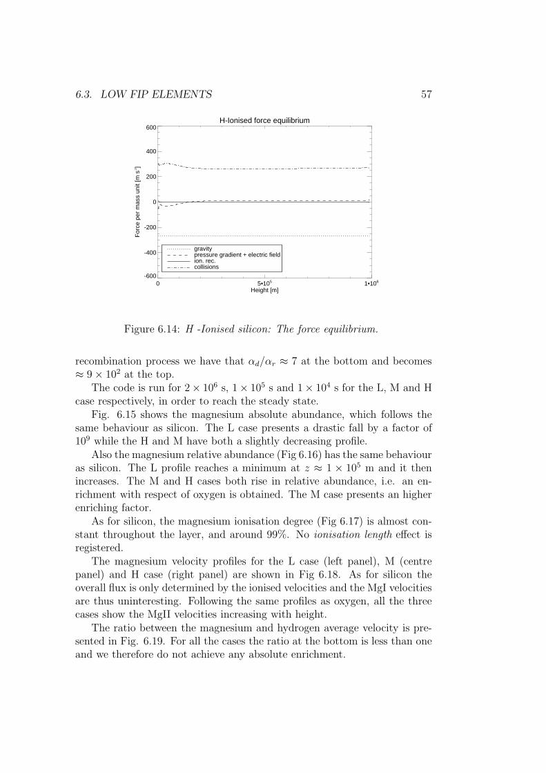
6.3. LOW FIP ELEMENTS 57
H-Ionised force equilibrium
0 5•105 1•106
Height [m]
-600
-400
-200
0
200
400
600
For
ce p
er m
ass
unit
[m s
-2]
collisionsion. rec.pressure gradient + electric fieldgravity
Figure 6.14: H -Ionised silicon: The force equilibrium.
recombination process we have that αd/αr ≈ 7 at the bottom and becomes≈ 9 × 10² at the top.
The code is run for 2× 10⁶ s, 1× 10⁵ s and 1× 10⁴ s for the L, M and Hcase respectively, in order to reach the steady state.
Fig. 6.15 shows the magnesium absolute abundance, which follows thesame behaviour as silicon. The L case presents a drastic fall by a factor of109 while the H and M have both a slightly decreasing profile.
Also the magnesium relative abundance (Fig 6.16) has the same behaviouras silicon. The L profile reaches a minimum at z ≈ 1 × 10⁵ m and it thenincreases. The M and H cases both rise in relative abundance, i.e. an en-richment with respect of oxygen is obtained. The M case presents an higherenriching factor.
As for silicon, the magnesium ionisation degree (Fig 6.17) is almost con-stant throughout the layer, and around 99%. No ionisation length effect isregistered.
The magnesium velocity profiles for the L case (left panel), M (centrepanel) and H case (right panel) are shown in Fig 6.18. As for silicon theoverall flux is only determined by the ionised velocities and the MgI velocitiesare thus uninteresting. Following the same profiles as oxygen, all the threecases show the MgII velocities increasing with height.
The ratio between the magnesium and hydrogen average velocity is pre-sented in Fig. 6.19. For all the cases the ratio at the bottom is less than oneand we therefore do not achieve any absolute enrichment.

58 CHAPTER 6. THE MINOR CONSTITUENTS
L
0 5•105 1•106
Height [m]
10-14
10-12
10-10
10-8
10-6
10-4
10-2
AA
BS []
H and M
0 5•105 1•106
Height [m]
0.0000
0.0001
0.0002
0.0003
0.0004
0.0005
AA
BS []
LMH
Figure 6.15: The magnesium absolute abundance.
L
0 5•105 1•106
Height [m]
10-6
10-5
10-4
10-3
10-2
10-1
100
AR
EL [
]
H and M
0 5•105 1•106
Height [m]
0.0
0.5
1.0
1.5
AR
EL [
]
LMH
Figure 6.16: The magnesium relative abundance.
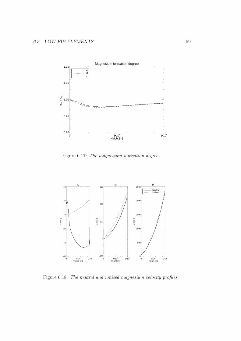
6.3. LOW FIP ELEMENTS 59
Magnesium ionisation degree
0 5•105 1•106
Height [m]
0.90
0.95
1.00
1.05
1.10
n MgI
I / N
Mg [
]
HML
Figure 6.17: The magnesium ionisation degree.
H
0 5•105 1•106
Height [m]
0
500
1000
1500
2000
2500
u [m
s-1]
NeutralIonised
M
0 5•105 1•106
Height [m]
-200
0
200
400
600
u [m
s-1]
L
0 5•105 1•106
Height [m]
-60
-40
-20
0
20
40
u [m
s-1]
Figure 6.18: The neutral and ionised magnesium velocity profiles.
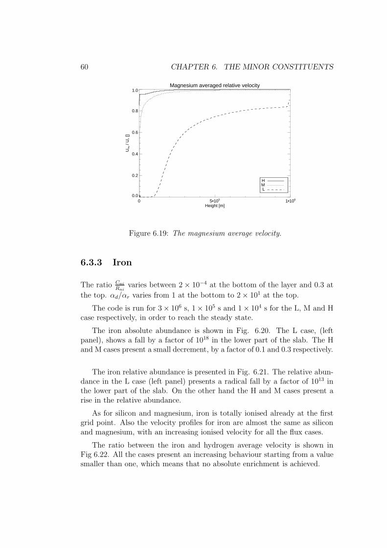
60 CHAPTER 6. THE MINOR CONSTITUENTS
Magnesium averaged relative velocity
0 5•105 1•106
Height [m]
0.0
0.2
0.4
0.6
0.8
1.0
UM
g / U
H []
LMH
Figure 6.19: The magnesium average velocity.
6.3.3 Iron
The ratio Cni
Rnivaries between 2 × 10⁻⁴ at the bottom of the layer and 0.3 at
the top. αd/αr varies from 1 at the bottom to 2 × 101 at the top.
The code is run for 3× 10⁶ s, 1× 10⁵ s and 1× 10⁴ s for the L, M and Hcase respectively, in order to reach the steady state.
The iron absolute abundance is shown in Fig. 6.20. The L case, (leftpanel), shows a fall by a factor of 1018 in the lower part of the slab. The Hand M cases present a small decrement, by a factor of 0.1 and 0.3 respectively.
The iron relative abundance is presented in Fig. 6.21. The relative abun-dance in the L case (left panel) presents a radical fall by a factor of 1013 inthe lower part of the slab. On the other hand the H and M cases present arise in the relative abundance.
As for silicon and magnesium, iron is totally ionised already at the firstgrid point. Also the velocity profiles for iron are almost the same as siliconand magnesium, with an increasing ionised velocity for all the flux cases.
The ratio between the iron and hydrogen average velocity is shown inFig 6.22. All the cases present an increasing behaviour starting from a valuesmaller than one, which means that no absolute enrichment is achieved.

6.3. LOW FIP ELEMENTS 61
L
0 5•105 1•106
Height [m]
10-25
10-20
10-15
10-10
10-5
100
AA
BS []
H and M
0 5•105 1•106
Height [m]
0.0000
0.0001
0.0002
0.0003
0.0004
0.0005
AA
BS []
LMH
Figure 6.20: The iron absolute abundance.
L
0 5•105 1•106
Height [m]
10-15
10-10
10-5
100
AR
EL [
]
H and M
0 5•105 1•106
Height [m]
0.0
0.2
0.4
0.6
0.8
1.0
1.2
1.4
AR
EL [
]
LMH
Figure 6.21: The iron relative abundance.

62 CHAPTER 6. THE MINOR CONSTITUENTS
Iron averaged relative velocity
0 5•105 1•106
Height [m]
0.0
0.2
0.4
0.6
0.8
1.0
UF
e / U
H []
LMH
Figure 6.22: The iron average velocity.
6.3.4 Discussion
For all the low FIP elements the gas is fully ionised already at the first gridpoint. This could mean that the grid dimensions are too large with respectto the ionisation space scale. The reason why we chose this grid was toreproduce the results of Peter (1998). Abundances values obtained with agrid with a higher resolution near the lower boundary are shown in chapter7 with similar results.
The adopted photoionisation rate (again taken form Peter (1998)) appearsquite unnatural with such a high rate that suddenly, at an arbitrary height,starts to work and ionises the gas totally. The results obtained with a moregradually growing ionisation rate are shown in section 7.2.3.
No absolute enrichment is obtained. In the H case the elements abun-dances present a small depletion (around 10%). The M case shows a strongerdepletion(≈ 40%), while in the L case the hydrogen wind does not manageto transport the minor constituent out of the layer, and the density of thelatter decays drastically by a factor of at least 1010. These results are instrong contrast with the high enrichment obtained by Peter (1998).
When it comes to the relative abundance, the low FIP elements showsome enrichment with respect to oxygen. In the H case the enrichment isabout 10%, and in the M case it gets larger (between 30% and 50%), while theL case shows a strong depletion of many order of magnitude. Neverthelessthe relative abundances are characterised by some rapid variations at the

6.4. NEON 63
L
0 5•105 1•106
Height [m]
10-25
10-20
10-15
10-10
10-5
100
AA
BS []
H and M
0 5•105 1•106
Height [m]
0.0000
0.0001
0.0002
0.0003
0.0004
0.0005
0.0006
AA
BS []
LMH
Figure 6.23: The neon absolute abundance.
lower boundary and the obtained relative enrichments are thus just artifacts,as it is shown with a further analysis in section 7.2.2.
6.4 Neon
The ionisation process for neon is strongly dominated by the radiative ion-isation. The ratio between the collisional and the radiative ionisation rate,Cni
Rni, varies between 10−11 at the bottom to 10−5 at the top. The radiative
recombination dominates the recombination process by factor larger than106.
In order to reach the steady state the code is run for 2 × 10⁶ s, 1 × 10⁵ sand 1 × 10⁴ s for the L, M and H case respectively.
6.4.1 Results
Fig. 6.23 shows the neon absolute abundance for the L case (left panel)and M and H cases (right panel). In the L case the absolute abundancefalls radically by a factor of 1017. Unlike the L case for oxygen and for thelow FIP elements, the neon L case shows a monotonous, almost exponentialbehaviour throughout the slab. While the M case presents a decreasingabsolute abundance the H case shows a rise of about 10% at lower altitude.
In Fig. 6.24 the neon relative abundances for the L case (left panel) and

64 CHAPTER 6. THE MINOR CONSTITUENTS
L
0 5•105 1•106
Height [m]
10-12
10-10
10-8
10-6
10-4
10-2
100
102
AR
EL [
]
H and M
0 5•105 1•106
Height [m]
0.0
0.5
1.0
1.5
2.0
AR
EL [
]
LMH
Figure 6.24: The neon relative abundance.
for the H and M cases (right panel) are shown. In the L case the relativeabundance falls by a factor of 1010 while in the H and M case we have arelative enrichment by a factor of 0.3 and 0.5 respectively. The rise of therelative abundance happens in the lower part of the slab, up to z ≈ 2.5×10⁵
m.The neon ionisation degree is presented in Fig. 6.25. The L and M cases
show an almost totally ionised gas already at the bottom of the slab. In the Hcase the ionisation length effect is visible and causes a delay in the ionisationdegree with respect to the L and M cases. Thus, with the adopted radiativeionisation rate, neon gets fully ionised much before oxygen and hydrogen,despite that it has an ionisation energy of ≈ 22 eV relative to 13.6 eV for Hand O.
The neutral and ionised neon velocities are shown in Fig. 6.26. As for thelow FIP elements, because of the high ionisation degree, the NeI velocitiesare insignificant, except for the H case at the lower boundary. Here the NeIvelocity is greater than the one of NeII. All the cases present a positive andmonotonous ionised velocity.
Since neon is not fully ionised throughout the slab, and since the neutralvelocities assume negative values, it is also interesting to study the neutraland ionised neon fluxes (Fig. 6.27). In the L case (left panel) the drasticdensity fall leads to almost zero fluxes, except at lower altitudes. Here neutralneon is streaming upward while ionised neon is falling. The M case (centrepanel) shows a high upward ionised flux, while the neutral neon is streaming

6.4. NEON 65
Neon ionisation degree
0 5•105 1•106
Height [m]
0.0
0.2
0.4
0.6
0.8
1.0
n NeI
I / N
Ne [
]
LMH
Figure 6.25: The neon ionisation degree.
H
0 5•105 1•106
Height [m]
0
500
1000
1500
2000
2500
u [m
s-1]
NeutralIonised
M
0 5•105 1•106
Height [m]
-500
0
500
1000
u [m
s-1]
L
0 5•105 1•106
Height [m]
-400
-300
-200
-100
0
100
u [m
s-1]
Figure 6.26: The neutral and ionised neon velocity profiles.

66 CHAPTER 6. THE MINOR CONSTITUENTS
H-flux
0 5•105 1•106
Height [m]
0
1•1015
2•1015
3•1015
4•1015
5•1015
u n
[m-2 s
-1]
M-flux
0 5•105 1•106
Height [m]
-2•1014
0
2•1014
4•1014
6•1014
8•1014
u n
[m-2 s
-1]
L-flux
0 5•105 1•106
Height [m]
-2•1012
-1•1012
0
1•1012
2•1012
u n
[m-2 s
-1]
IonisedNeutral
Figure 6.27: The neutral and ionised neon fluxes.
downward and constitutes a small part of the total flux at lower altitudes.In the H case (right panel) the neutral flux is slightly less significant andpositive throughout the slab.
Fig. 6.28 shows the ratio between the neon and hydrogen relative velocity.For the H flux the ratio can appear slightly larger than one at the bottom,leading to a possible enrichment. In the L case the ratio is almost zero givingthe net result that no neon is dragged up by hydrogen.
The force equilibrium for neutral and ionised neon in the H case is shownin Fig. 6.29. For NeI, the force equilibrium is characterised by a balancebetween gravity and collisions with hydrogen throughout the slab except fornear the lower boundary. Here an upward pressure gradient force arises, bal-anced by the sum of gravity and collisions. At the very beginning of thelayer, in order to balance the pressure gradient, the collision force becomesnegative and the NeI velocities become thus higher than the hydrogen ve-locities. These high NeI velocities justify a Ne average velocity larger thanhydrogen at the lower boundary. For NeII the picture is the same exceptat the lower boundary where a negative pressure gradient force is balancedby a high upward collisional force. To obtain such an upward force the NeIIvelocities must be lower than the hydrogen ones.

6.4. NEON 67
Neon averaged relative velocity
0 5•105 1•106
Height [m]
0.0
0.2
0.4
0.6
0.8
1.0
1.2
UN
e / U
H []
LMH
Figure 6.28: The neon average velocity.
H-Neutral force equilibrium
0 5•105 1•106
Height [m]
-600-400
-200
0
200
400600
For
ce p
er m
ass
unit
[m s
-2]
H-Ionised force equilibrium
0 5•105 1•106
Height [m]
-1500-1000
-500
0
500
10001500
For
ce p
er m
ass
unit
[m s
-2]
gravitypressure gradient + electric fieldion. rec.collisions
Figure 6.29: H - Neon: The force equilibrium.
68 CHAPTER 6. THE MINOR CONSTITUENTS
6.4.2 Discussion
The H case for neon is quite interesting because the ionisation length effectis visible and a growing ionisation degree is achieved. This steep ionisationdegree builds an upward pressure gradient force for NeI and a respectivedownward force for NeII. Since NeII is coupled to protons by a stronger colli-sional force the overall neon average velocity becomes larger than hydrogen.This velocity gives a very small (less than 10%) but visible absolute enrich-ment (if we do not account for the negative spike in the average velocity atthe lower boundary).
Neon is a high FIP element and no enrichment should thus be obtained.This anomaly is probably due to the fact that in our model, using the ionisa-tion rate by Peter (1998), neon gets ionised much before hydrogen. Howeverthis result shows that with a steep ionisation degree a small enrichment canbe obtained. In section 7.2.1 we check the possibility to obtain such or maybelarger enrichment for the low FIP elements.

Chapter 7
Discussion
7.1 The background model
The results obtained in chapter 5 can be compared with the hydrogen back-ground model of Peter and Marsch (1998). The largest difference betweenthese models can be found in the choice of the boundary conditions. InPeter and Marsch (1998) the velocities for neutral and ionised hydrogen areforced to be equal not only at the top (as we do in our model) but also at thebottom. They give reasons for this choice by claiming that charge exchangeand ionisation-recombination keep a tight collisional coupling between thecharge states. As we have studied in eq. 5.7 an increasing ionisation rateleads to a velocity difference between the neutral and the ionised specie.Therefore forcing equal velocity at the bottom, where the ionisation rateincreases, could be inappropriate. Another difference is that in our modelwe force a solar wind flux through the layer by a choice of the boundaryconditions, while Peter and Marsch (1998) obtain such flux from the modelitself. This means that in their model they claim that solar wind is a “prod-uct” of the chromosphere, whereas in our model the process that determinesthe solar wind mass flux is placed somewhere else above this chromosphericionisation layer.
7.2 The minor constituents model
7.2.1 Searching for enrichment
Peter (1998) obtained a significant absolute fractionation for many minorconstituents, whereas in this work no enrichment relative to hydrogen wasfound (except a small enrichment for one isolated case). The largest difference
69

70 CHAPTER 7. DISCUSSION
Ionisation degree
0 1•104 2•104
Height [m]
0.7
0.8
0.9
1.0
1.1
n i /
n n []
ion. equi.ion. deg.
Neutral and ionised densities
0 1•104 2•104
Height [m]
0
5.0•1013
1.0•1014
1.5•1014
2.0•1014
n x [m
-3]
SiIISiI
Figure 7.1: The silicon ionisation degree(left panel) and the SiI together withSiII densities in H case, plotted for the ionisation area, using Peter’s bound-ary conditions and a higher resolution grid.
between Peter’s approach and ours is represented by his coupling betweenthe ionised and neutral minor constituent velocity, not only at the top butalso at the bottom of the layer.
Another important aspect that needs more attention is the ionisationrate. The photoionisation rate from Peter (1998) (see section 2.1.1) for theminor constituents leads to a sudden and drastic ionisation. The respectiveionisation length is therefore getting quite small. For example, silicon in theH flux case has LION ≈ 102 m, that is 25 times smaller than the adopted gridspacing. Therefore in order to study this thin area, where the fractionationprocesses are believed to take place, a higher resolution grid (smaller gridspacing) is needed. We thus define a new grid where the grid points, instead ofbeing distributed homogeneously, cover the ionisation area with a resolutionthat is higher than in the rest of the grid. In that way we are sure not tomiss any important effect happening in the lower part of the grid.
We now want to study how and if (by using a higher resolution gridtogether with Peter’s boundary conditions) any enrichment can really beobtained. The boundary conditions are thus modified as described above,both in the background and in the minority code. In the first part of thegrid, up to z = 2× 10⁴ m, the grid spacing is reduced by a factor of 100. Wenow present the results obtained for silicon in the H flux case.
The left panel of Fig. 7.1 shows the ionisation degree and the ionisation

7.2. THE MINOR CONSTITUENTS MODEL 71
Fluxes:Ionisation area
0 1•104 2•104
Height [m]
0
5.0•1015
1.0•1016
1.5•1016
2.0•1016u
n [m
-2 s
-1]
SiISiII
Figure 7.2: The neutral and ionised silicon fluxes in the H case, plotted forthe ionisation area, using Peter’s boundary conditions and a higher resolutiongrid.
equilibrium obtained for silicon near the lower boundary, while the rightpanel shows the SiI and SiII densities. Even if we use a grid spacing that issmaller than the theoretical ionisation length, and even if the in-streaminggas is only 1% ionised, silicon is highly ionised (≈ 80%) already from thefirst grid point. However, a small ionisation length effect is visible at thevery beginning of the layer.
The real effect of ionisation can be studied from the continuity equation,where we observe that in a steady state we have non-zero spatial derivativesof a particle flux only at those heights where the ionisation-recombinationprocess is taking place. In other words, if the flux for SiI (or in the sameway for SiII) does not show any spatial variation, the sum of the ionisationand recombination net effect is negligible. Analysing these fluxes, shown inFig. 7.2, we see that the ionisation process is taking place from the lowerboundary up to z = 3 × 10³ m. This means that the ionisation process isdelayed as described by the ionisation length concept, but when it comesto the real ionisation degree, nSiII/(nSiI + nSiII), this delay in ionisation isalmost not visible.
A reason for this can be found in the SiI and SiII velocities at the bottom,displayed in Fig 7.3. At the lower boundary the velocities are forced to beequal, but already from the second grid point the two velocity profiles areseparated by a huge gap. When the in-streaming neutral silicon gets ionised,

72 CHAPTER 7. DISCUSSION
Silicon velocities
0 1•104 2•104
Height [m]
0
100
200
300
400
500
u [m
s-1]
SiISiII
Figure 7.3: The neutral and ionised silicon velocities in the H, plotted for theionisation area, using Peter’s boundary conditions and a higher resolutiongrid.
its velocity falls to a near zero value, and then it increases slowly. In thatway SiII can accumulate and the overall ionisation degree becomes as shownin Fig. 7.1 The ionisation delay due to the ionisation length concept istherefore strongly reduced. From this picture it also sounds quite unphysicalto force the HI and HII velocities to be equal right where the ionisation takesplace, because at those heights the pressure gradients for HI and HII givetwo opposite effects.
The force equilibrium is shown in detail in Fig. 7.4. The high SiI velocityat the bottom is caused by an upward pressure gradient force, which arisesfrom a decreasing SiI density near the lower boundary. On the other hand SiIIis subject to a downward pressure gradient force, balanced by the collisionalfriction. This pressure gradient is again caused by a SiII density increasingwith height.
Finally, from Fig 7.5 we see that the average velocity for silicon at thelower boundary is greater than the hydrogen average velocity. Due to eq.4.10, this leads to an enrichment that can also be observed as an increasein the absolute abundance from the lower boundary value of 5 × 10⁻⁴ to6 × 10−4.
Summarising this section, we have seen that even if we use a high enoughprecision in the grid we obtain a quite limited ionisation area where the minorconstituent is already 80% ionised at the first grid point. This shows that

7.2. THE MINOR CONSTITUENTS MODEL 73
Ionisation area - SiI
0 1•104 2•104
Height [m]
-6000-4000
-2000
0
2000
40006000
For
ce p
er m
ass
unit
[m s
-2]
Ionisation area - SiII
0 1•104 2•104
Height [m]
-6000-4000
-2000
0
2000
40006000
For
ce p
er m
ass
unit
[m s
-2]
gravitypressure gradient + electric fieldcharge exchangecollisions
Figure 7.4: The neutral silicon (upper panel) and ionised silicon (lower panel)force equilibrium in the H case, plotted for the ionisation area, using Peter’sboundary conditions and a higher resolution grid.
Average velocity:Ionisation area
0 1•104 2•104
Height [m]
0.4
0.6
0.8
1.0
1.2
1.4
1.6
US
i / U
H []
Average velocity:Whole grid
0 5•105 1•106
Height [m]
0.4
0.6
0.8
1.0
1.2
1.4
1.6
US
i / U
H []
Figure 7.5: The ratio between the silicon and the hydrogen average velocity,plotted for the ionisation area (left panel) and for the whole grid (right panel)in the H case,using Peter’s boundary conditions and a higher resolution grid.

74 CHAPTER 7. DISCUSSION
Ionisation degree
0 5.0•103 1.0•104 1.5•104 2.0•104
Height [m]
0.0
0.2
0.4
0.6
0.8
1.0
n SiII /
NS
i []
ionisation degreeionisation equilibrium
Figure 7.6: The silicon ionisation degree and ionisation equilibrium plottedfor the ionisation area.
the ionisation length simplification, used as a fundamental process by Peter(1998), does not give a correct picture of the ionisation dynamic. However,the remaining 20% of the ionisation process manages to build a pressuregradient that increases the average velocity of the minor constituent up to avalue a bit higher than the hydrogen average velocity, leading to a very smallenrichment.
7.2.2 Additional results
We now want to verify if the very small enrichment obtained in the previoussection is a real process that can explain the FIP effect, or if it only is an eventthat depends on the choice of some parameters like the boundary conditions.We move the ionisation area up to a height of zion = 1.5× 10⁴ m by turningon the photoionisation rate for minor constituents at z = zion instead of atthe lower boundary z = 0 m. This allows us to study what happens belowthe radical increase of the photoionisation rate, and the solution we obtainis less dependent of an arbitrary choice for the boundary conditions.
The results for the H flux case for silicon, with the described modificationsand with our boundary conditions, are presented below.
Fig. 7.6 shows the ionisation degree for silicon, plotted together with theionisation equilibrium (see eq. 5.4). The latter, following the photoionisationrate, has a constant value of 1% from the lower boundary up to z = 1.5×10⁴

7.2. THE MINOR CONSTITUENTS MODEL 75
Ionisation area
0 1•104 2•104
Height [m]
0
100
200
300
400
500
u [m
s-1]
SiISiII
Whole grid
0 5•105 1•106
Height [m]
0
500
1000
1500
2000
2500
u [m
s-1]
Figure 7.7: The neutral and ionised silicon velocities, plotted for the ionisa-tion area (left panel) and for the whole grid (right panel).
m, where it makes a discrete jump increasing to 100% and it then keeps thisvalue for the rest of the grid. The actual ionisation degree shows a smootherbehaviour. Its value is higher than equilibrium value below the height of thephotoionisation “ignition” and lower than the equilibrium value above thisheight.
We note that Fig. 7.1 is quite similar to Fig. 7.6 if we shift the latter tothe left by a distance ∆z = 1.5 × 10⁴ m.
By studying the SiI flux we can measure the ionisation length, obtainingLION ≈ 2 × 10² m. However, the real length (and time) needed by the gasto become half ionised, is much larger (≈ 4 × 10³ m). This is caused bythe dynamic following a high velocity difference between neutral and ionisedsilicon, as shown in Fig. 7.7.
The neutral silicon velocity shows a sudden rise followed by a similarfall, located at the height of the rate ignition, whereas the ionised siliconvelocity has a smaller magnitude dip at the same height. These featuresdo not influence the velocities for the rest of the grid, where both the SiIand SiII velocities increase at the same rate. The ionisation process thusappears just as a local event that does not modify the velocity at the top(or at the bottom) of the grid. Furthermore, this result is in agreement withwhat we found with the old grid (see right panel of Fig. 6.12), except for themagnitude of the spike near the lower boundary, and therefore legitimatesthe results of chapter 6.

76 CHAPTER 7. DISCUSSION
Absolute abundance:Ionisation area
0 1•104 2•104
Height [m]
0.0000
0.0002
0.0004
0.0006
AA
BS []
Absolute abundance:Whole grid
0 5•105 1•106
Height [m]
0.0000
0.0002
0.0004
0.0006
AA
BS []
Average velocity:Ionisation area
0 1•104 2•104
Height [m]
0.0
0.5
1.0
1.5
2.0
US
i / U
H []
Average velocity:Whole grid
0 5•105 1•106
Height [m]
0.0
0.5
1.0
1.5
2.0
US
i / U
H []
Figure 7.8: The ratio between the silicon and the hydrogen average velocity(upper panels), plotted for the ionisation area (left panel) and for the wholegrid (right panel).
The ratio between the silicon and hydrogen average velocity is shown inthe upper panels of Fig. 7.8. The sum of the SiI and SiII velocities givesa positive rise in the average velocity. However, as already mentioned, thisfeature does not modify the overall velocity behaviour (right panel). Hence,except for the ionisation area, the silicon average velocity is less than thehydrogen velocity, also at the bottom of the grid. This means that a realfractionation process does not take place, but rather a local depletion.
The overall absolute abundance shows a depletion from the lower bound-ary value 5 × 10⁻⁴ to a value 4 × 10⁻⁴ at the top of the grid. This is due toflux conservation and the increasing of silicon velocities. In fact, before a fullcoupling between silicon and hydrogen is reached, the silicon velocities arelower than the hydrogen velocities. Also the dip in the absolute abundanceproceeds from the total flux conservation and from the average velocity pro-file. The latter can be understood by studying the force equilibrium shownin Fig. 7.9.
The force equilibrium for SiI in the ionisation area (upper left panel of Fig.7.9) presents a high pulse of the pressure gradient caused by the decreasing SiIdensity in the ionisation process. This upward pressure gradient force leadsto an increase of the SiI velocities. A collisional friction with the hydrogenbackground therefore arises and balances this pressure gradient. For SiIIthe force balance (lower left panel of Fig. 7.9) shows an opposite symmetry,
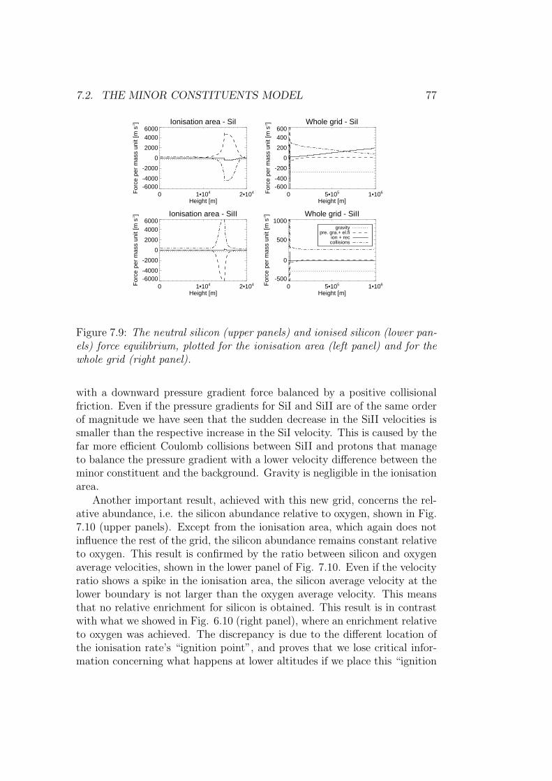
7.2. THE MINOR CONSTITUENTS MODEL 77
Ionisation area - SiI
0 1•104 2•104
Height [m]
-6000-4000
-2000
0
2000
40006000
For
ce p
er m
ass
unit
[m s
-2] Whole grid - SiI
0 5•105 1•106
Height [m]
-600-400
-200
0
200
400600
For
ce p
er m
ass
unit
[m s
-2]
Ionisation area - SiII
0 1•104 2•104
Height [m]
-6000-4000
-2000
0
2000
40006000
For
ce p
er m
ass
unit
[m s
-2] Whole grid - SiII
0 5•105 1•106
Height [m]
-500
0
500
1000
For
ce p
er m
ass
unit
[m s
-2]
gravitypre. gra.+ el.fi
ion + reccollisions
Figure 7.9: The neutral silicon (upper panels) and ionised silicon (lower pan-els) force equilibrium, plotted for the ionisation area (left panel) and for thewhole grid (right panel).
with a downward pressure gradient force balanced by a positive collisionalfriction. Even if the pressure gradients for SiI and SiII are of the same orderof magnitude we have seen that the sudden decrease in the SiII velocities issmaller than the respective increase in the SiI velocity. This is caused by thefar more efficient Coulomb collisions between SiII and protons that manageto balance the pressure gradient with a lower velocity difference between theminor constituent and the background. Gravity is negligible in the ionisationarea.
Another important result, achieved with this new grid, concerns the rel-ative abundance, i.e. the silicon abundance relative to oxygen, shown in Fig.7.10 (upper panels). Except from the ionisation area, which again does notinfluence the rest of the grid, the silicon abundance remains constant relativeto oxygen. This result is confirmed by the ratio between silicon and oxygenaverage velocities, shown in the lower panel of Fig. 7.10. Even if the velocityratio shows a spike in the ionisation area, the silicon average velocity at thelower boundary is not larger than the oxygen average velocity. This meansthat no relative enrichment for silicon is obtained. This result is in contrastwith what we showed in Fig. 6.10 (right panel), where an enrichment relativeto oxygen was achieved. The discrepancy is due to the different location ofthe ionisation rate’s “ignition point”, and proves that we lose critical infor-mation concerning what happens at lower altitudes if we place this “ignition

78 CHAPTER 7. DISCUSSION
Relative abundance:Ionisation area
0 1•104 2•104
Height [m]
0.00.2
0.4
0.6
0.8
1.01.2
AR
EL [
]
Relative abundance: Whole grid
0 5•105 1•106
Height [m]
0.00.2
0.4
0.6
0.8
1.01.2
AR
EL [
]
Average velocities:Ionisation area
0 1•104 2•104
Height [m]
0
50
100
150
200
U [m
s-1]
OxygenSilicon
Velocities ratio:Whole grid
0 5•105 1•106
Height [m]
0.0
0.5
1.0
1.5
2.0
2.5
US
i / U
O []
Figure 7.10: The silicon relative abundance (upper panels) plotted for theionisation area (left panel) and for the whole grid (right panel). The siliconand oxygen average velocities (lower panels) in the ionisation area. The ratiobetween silicon and oxygen average velocities for the whole grid (right panel).
point” at the lower boundary.
In this section we have seen that a steep ionisation degree leads to a fall inthe abundance, located exactly at the ionisation height zion, followed imme-diately by an analog rise of the abundance. This means that the abundancevariations measured with respect to this low value can appear like an enrich-ment (see previous paragraph), but at the same time these ionisation areaabundance values are depleted with respect to photospheric values (repre-sented by the lower boundary). No real enrichment is therefore achieved. Inother words, because the ionisation process causes a local density depletion,comparing abundance values from higher altitudes with the abundance valueat zion will give an unreal enrichment.
The area where the minor constituent velocity exceeds the hydrogen veloc-ity is characterised by a pressure gradient force due to the ionisation process.Below this area no force can provide for such a high velocity. Since collisionsconstitute the only force that balances gravity, the minor constituent averagevelocity must be lower than the hydrogen velocity, both above and below theionisation area.

7.2. THE MINOR CONSTITUENTS MODEL 79
Ionisation degree
0 5•105 1•106
Height [m]
0.0
0.2
0.4
0.6
0.8
1.0
n XII /
NX []
HydrogenNeon
Silicon
Figure 7.11: A gradually growing ionisation degree for silicon, hydrogen andneon, in the H flux case.
7.2.3 Gradual ionisation
As already mentioned (see section 6.3.4), the adopted photoionisation rate,characterised by a sudden and drastic increase, is quite unphysical. Thisionisation is caused by radiation coming from the above corona, but theionising radiation stops to work at the lower boundary or at a so-called“ignition point”, and no gas is ionised below this wall.
We now want to check if any fractionation process can be obtained with amore likely ionisation degree. We build a gradual ionisation rate and run thecode for the H case for silicon, oxygen and neon. Fig. 7.11 shows the gradu-ally growing ionisation degree for silicon and neon, compared with hydrogen.With the new ionisation rate silicon becomes ionised before hydrogen whileneon becomes ionised after it.
Fig. 7.12 shows the average velocity of silicon and neon relative to hydro-gen (left panel), and relative to oxygen (right panel), in the H flux case. Thevalue, ≈ 0.8, of the average silicon velocity relative to hydrogen at the lowerboundary leads to a depletion in absolute abundance by 20%, while the ab-solute neon abundance is depleted by a factor of 40%. These values confirmwhat we found in section 7.2.2, and show that also with a gradual ionisa-tion no enrichment is obtained. When it comes to the relative abundance,silicon has the same velocity as oxygen at the lower boundary and thus noenrichment is obtained, even if the earlier ionisation of silicon causes a rise,
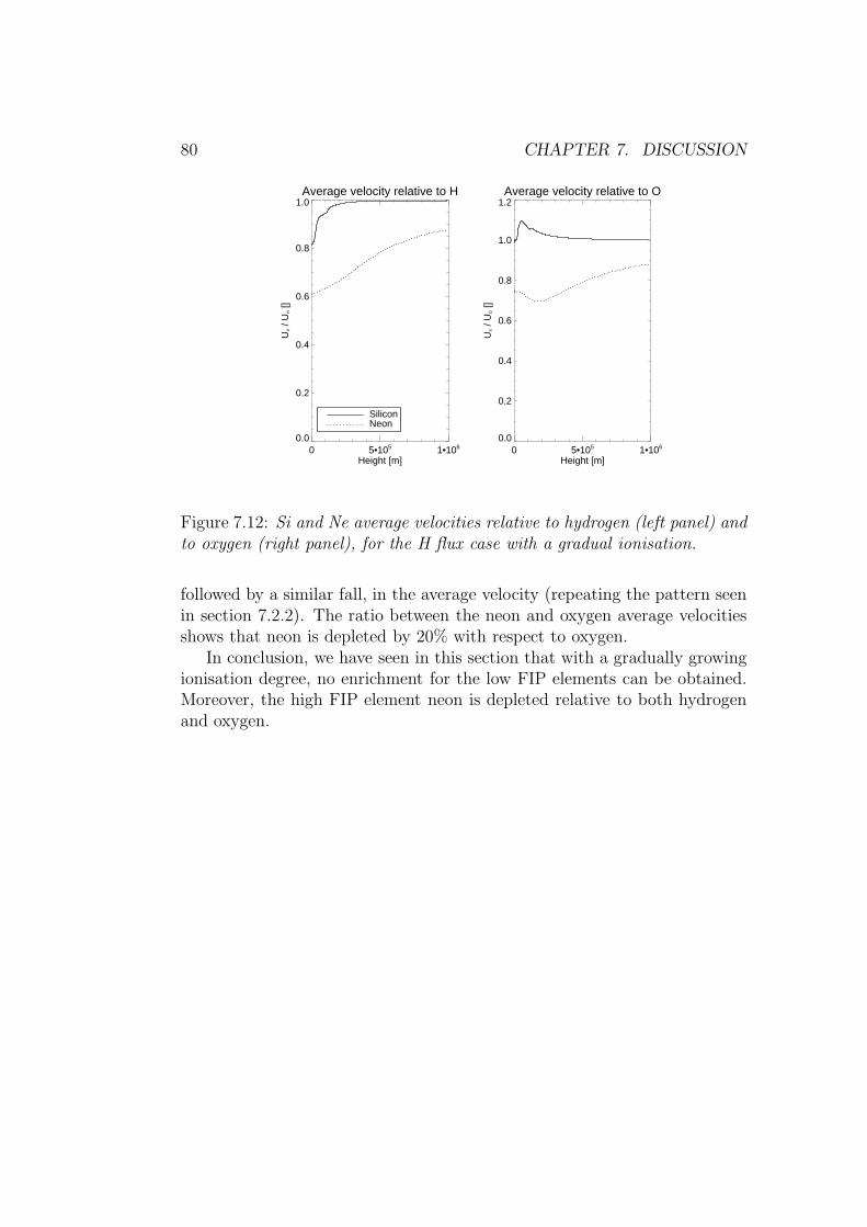
80 CHAPTER 7. DISCUSSION
Average velocity relative to H
0 5•105 1•106
Height [m]
0.0
0.2
0.4
0.6
0.8
1.0
UX /
UH []
NeonSilicon
Average velocity relative to O
0 5•105 1•106
Height [m]
0.0
0.2
0.4
0.6
0.8
1.0
1.2
UX /
UO []
Figure 7.12: Si and Ne average velocities relative to hydrogen (left panel) andto oxygen (right panel), for the H flux case with a gradual ionisation.
followed by a similar fall, in the average velocity (repeating the pattern seenin section 7.2.2). The ratio between the neon and oxygen average velocitiesshows that neon is depleted by 20% with respect to oxygen.
In conclusion, we have seen in this section that with a gradually growingionisation degree, no enrichment for the low FIP elements can be obtained.Moreover, the high FIP element neon is depleted relative to both hydrogenand oxygen.

Chapter 8
Summary
In-situ observations together with spectroscopic measurements show that theelemental composition of the solar atmosphere varies from the photosphere tosolar wind. An enrichment by a factor of 2 or more for the low FIP elementsrelative to oxygen (and with larger uncertainty also relative to hydrogen) hasbeen found.
Many models have been implemented in order to explain this fractiona-tion. In this work we have followed the same approach as Peter (1998) andtried to repeat his results concerning the FIP effect in fast solar wind.
A background model that describes a layer of the chromosphere wherehydrogen is the only constituent, has been implemented. The obtainedresults for the hydrogen background are substantially in agreement withPeter and Marsch (1998), who provide the background model for Peter (1998).
A second model that describes minor constituents in such a backgroundhas also been made. This minor constituent model has been run for differentparameter values (like the wind flux) and with different boundary conditions.
No enrichment comparable to the ones achieved by Peter (1998) has beenfound for the low FIP elements. A downward pressure gradient force arisesand brakes the ionised specie so that this can pile up at the lower boundaryand oppose the formation of a steep ionisation degree. However, if a steepenough ionisation degree is somehow built at the lower boundary, an upwardpressure gradient force acting on the neutral specie can arise. In that waya small enrichment, definitively smaller than the results of Peter (1998), isobtained.
Furthermore, a new and perhaps more important result have been ob-tained by moving the ionisation area away from the lower boundary: at theionisation height the minor constituent abundance reaches a local minimum.It is therefore incorrect to adopt this minimum as the reference photosphericvalue when evaluating the enrichment.
81

82 CHAPTER 8. SUMMARY
This result is just the validation of a simple physical line of reasoning.In order to transport these heavy ions out of the gravitational field an up-ward force able to balance gravity is needed. If this force is represented bycollisions with hydrogen the minor constituent velocity must be lower thanthe hydrogen velocity, and no enrichment can be obtained. If instead thisupward force is constituted by the pressure gradient force caused by the ion-isation process, no high velocity will be obtained outside the ionisation area,and hence no real enrichment can be obtained. Let’s say that the ionisationprocess provides the minor constituent with this upward force (that drivesthe trace gas with a velocity higher than hydrogen). In order to keep thishigh velocity and thus obtain a real enrichment, a pressure gradient able atleast to balance gravity must arise all the way down from the ionisation areato the photosphere. In such a way, because of the large height scale of theminor constituent, the density will drop so much that almost no particleswill be left in the solar wind.
This work has thus confirmed that the ionisation-diffusion process sug-gested by Peter (1998) as a pure steady-state mechanism, cannot account forthe observed FIP effect in the solar wind.
A further work could study a time-dependent process where a regularlyrepeated mixing keeps the chromospheric abundance at photospheric values.It is necessary to investigate how this mixing process can interact with theionisation-diffusion mechanism and whether or not an enrichment of the lowFIP elements can be achieved.
A l’alta fantasia qui manco possa;ma gia volgeva il mio disio e ’l velle,sı come rota ch’igualmente e mossa,
l’amor che move il sole e l’altre stelle.
Here vigour failed the lofty fantasy:But now was turning my desire and will,
Even as a wheel that equally is moved,The Love which moves the sun and the other stars.
Dante Alighieri

Bibliography
Abramowitz, M. and Stegun, I. A. (1964). Handbook of mathematical func-tions. U.S. Department of Commerce, third edition.
Arnaud, M. and Raymond, J. (1992). Iron ionization and recombinationrates and ionization equilibrium. ApJ, 398:394–406.
Arnaud, M. and Rothenflug, R. (1985). An updated evaluation of recombi-nation and ionization rates. A&AS, 60:425–457.
Asplund, M., Grevesse, N., Sauval, A. J., Allende Prieto, C., and Kiselman,D. (2004). Line formation in solar granulation. IV. [O I], O I and OH linesand the photospheric O abundance. A&A, 417:751–768.
Banks, P. M. and Kockarts, G. (1973). Aeronomy. Academic Press, Inc. NewYork.
Byhring, H. S., Esser, R., and Lie-Svendsen, Ø. (2008). The Funnel Geometryof Open Flux Tubes in the Low Solar Corona Constrained by O VI andNe VIII Outflow. ApJL, 673:L91–L94.
Feldman, U. and Laming, J. M. (2000). Element Abundances in the Up-per Atmospheres of the Sun and Stars: Update of Observational Results.Physica Scripta, 61:222–+.
Gray, D. F. (2005). The observation and analysis of the stellar atmospheres.Cambridge University Press, New York.
Grevesse, N. and Sauval, A. J. (1998). Standard Solar Composition. SpaceScience Reviews, 85:161–174.
Henoux, J. C. and Somov, B. V. (1997). The photospheric dynamo. I. Physicsof thin magnetic flux tubes. A&A, 318:947–956.
Hummer, D. G. (1983). The generalized exponential-integral. Journal ofQuantitative Spectroscopy and Radiative Transfer, 30:281–287.
83

84 BIBLIOGRAPHY
Korevaar, P. and van Leer, B. (1988). Time-dependent corona models - Anumerical method. A&A, 200:153–167.
Marsch, E., von Steiger, R., and Bochsler, P. (1995). Element fractionationby diffusion in the solar chromosphere. A&A, 301:261–+.
Peter, H. (1998). Element fractionation in the solar chromosphere driven byionization-diffusion processes. A&A, 335:691–702.
Peter, H. and Marsch, E. (1998). Hydrogen and helium in the solar chromo-sphere: a background model for fractionation. A&A, 333:1069–1081.
Press, W., S.A.Teukolsky, Vetterling, W., and Flannery, B. (1992). NumericalRecipes in Fortran 77. Cambridge University Press.
Russell, H. N. (1929). On the Composition of the Sun’s Atmosphere. ApJ,70:11–+.
Schultz, D. R., Krstic, P. S., Lee, T. G., and Raymond, J. C. (2008). Mo-mentum Transfer and Viscosity from Proton-Hydrogen Collisions Relevantto Shocks and Other Astrophysical Environments. ApJ, 678:950–960.
Schunk, R. W. (1977). Mathematical structure of transport equations formultispecies flows. Reviews of Geophysics and Space Physics, 15:429–445.
Shull, J. M. and van Steenberg, M. (1982). The ionization equilibrium ofastrophysically abundant elements. ApJS, 48:95–107.
Vauclair, S. (1996). Element segregation in the solar chromosphere and theFIP bias: the ”Skimmer” model. A&A, 308:228–232.
Vernazza, J. E., Avrett, E. H., and Loeser, R. (1981). Structure of thesolar chromosphere. III - Models of the EUV brightness components of thequiet-sun. ApJS, 45:635–725.
von Steiger, R. and Geiss, J. (1989). Supply of fractionated gases to thecorona. A&A, 225:222–238.
von Steiger, R. and Schwadron, N. A. (2000). Solar Wind Composition. InRamaty, R. and Mandzhavidze, N., editors, High Energy Solar PhysicsWorkshop - Anticipating Hess!, volume 206 of Astronomical Society of thePacific Conference Series, pages 54–+.
von Steiger, R., Schweingruber, R. F. W., Geiss, J., and Gloeckler, G. (1995).Abundance variations in the solar wind. Advances in Space Research, 15:3–.

BIBLIOGRAPHY 85
Wang, Y.-M. (1996). Element Separation by Upward Proton Drag in theChromosphere. ApJL, 464:L91+.