ENDANGERED SPECIES RESEARCHEndang Species Res

Vol. 14: 157–169, 2011doi: 10.3354/esr00344

Published online August 11

INTRODUCTION

From a legal perspective, it has recently been recog-nised that the relationship between the protection ofcetaceans within the European Union (EU) on the onehand and the EU Common Fisheries Policy on the otherconstitutes a classic example of a user–environmentconflict (Proelss et al. 2011). A similar problem mightarise in the near future with the construction of moreoffshore wind farms (OWFs) in Europe (Gill 2005),

which is clearly an important response to global warm-ing and is in line with the obligation to move to renew-able energy generation. Coastal zones, however, arealready under significant pressure from human activ-ity, and harbour porpoises Phocoena phocoena inhab-iting shelf waters are threatened by by-catch in fish-eries (Vinther & Larsen 2004, Siebert et al. 2006),chemical (Siebert et al. 1999, Das et al. 2006, Beinekeet al. 2007) and noise pollution (Richardson et al. 1995,Koschinski et al. 2003, Lucke et al. 2008, 2009). The

© Inter-Research 2011 · www.int-res.com*Email: gilles@ftz-west.uni-kiel.de

Modelling harbour porpoise seasonal density as afunction of the German Bight environment:

implications for management

Anita Gilles1,*, Sven Adler1,2, Kristin Kaschner1,3, Meike Scheidat1,4, Ursula Siebert1

1Research and Technology Centre (FTZ), Christian-Albrechts-University of Kiel, 25761 Büsum, Germany2University of Rostock, Institute for Biodiversity, 18057 Rostock, Germany

3Evolutionary Biology & Ecology Lab, Institute of Biology I (Zoology), Albert-Ludwigs-University, 79104 Freiburg, Germany4Wageningen IMARES, Institute for Marine Resources and Ecosystem Studies, Postbus 167, 1790 AD Den Burg,

The Netherlands

ABSTRACT: A classical user–environment conflict could arise between the recent expansion plans ofoffshore wind power in European waters and the protection of the harbour porpoise Phocoena pho-coena, an important top predator and indicator species in the North Sea. There is a growing demandfor predictive models of porpoise distribution to assess the extent of potential conflicts and to supportconservation and management plans. Here, we used a range of oceanographic parameters and gen-eralised additive models to predict harbour porpoise density and to investigate seasonal shifts in por-poise distribution in relation to several static and dynamic predictors. Sightings were collected duringdedicated line-transect aerial surveys conducted year-round between 2002 and 2005. Over the 4 yr,survey effort amounted to 38 720 km, during which 3887 harbour porpoises were sighted. Porpoisesaggregated in distinct hot spots within their seasonal range, but the importance of key habitatdescriptors varied between seasons. Predictors explaining most of the variance were the hydrograph-ical parameter ‘residual current’ and proxies for primary production and fronts (chlorophyll and nutri-ents) as well as the interaction ‘distance to coast/water depth’. Porpoises preferred areas withstronger currents and concentrated in areas where fronts are likely. Internal cross-validation indi-cated that all models were highly robust. In addition, we successfully externally validated our sum-mer model using an independent data set, which allowed us to extrapolate our predictions to a moreregional scale. Our models improve the understanding of determinants of harbour porpoise habitat inthe North Sea as a whole and inform management frameworks to determine safe limits of anthro-pogenic impacts.

KEY WORDS: Habitat modelling · Phocoena phocoena · Conservation · Generalised additive model ·North Sea

Resale or republication not permitted without written consent of the publisher

Contribution to the Theme Section ‘Beyond marine mammal habitat modeling’ OPENPEN ACCESSCCESS

Endang Species Res 14: 157–169, 2011

harbour porpoise is among the most common ce -taceans in the northern hemisphere (Hammond et al.2002) and as such is an important top predator andindicator species. Changes in the environment arelikely to be accommodated more readily by abundanttop predators than by many other species. Particularlythe construction of OWFs might have an impact, assource levels of pile driving are well above the audi-tory tolerance of P. phocoena (Lucke et al. 2009), andtheir zone of responsiveness (sensu Richardson et al.1995) extends beyond 20 km (Gilles et al. 2009,Tougaard et al. 2009). All North Sea coastal states havemajor plans to increase their marine renewable energyproduction (e.g. in the German North Sea, 23 OWFsare already approved and 57 additional sites are in theapproval process; see www.bsh.de/de/Meeresnutzung/Wirtschaft/CONTIS-Informationssystem/ContisKarten/NordseeOffshoreWindparksPilotgebiete.pdf; Fig. 1);within the next decade, construction activities will be

carried out at several locations simultaneously, andthese cumulative effects — in addition to recognisedthreats such as by-catch — can no longer be consideredshort term.

Moreover, the construction sites of several OWFsoverlap spatially with marine special areas of conser-vation (SACs) designated under the EU Habitats Direc-tive (Scheidat et al. 2006, Gilles et al. 2009), wherePhocoena phocoena is listed in Annex II and IV. SACsare supposed to include the main core range of anational stock (Wilson et al. 2004), but the delimitationof SACs is challenging for highly mobile species suchas the harbour porpoise (Embling et al. 2010). Animportant prerequisite for the implementation of asound management plan for the entire North Sea istherefore the identification of hotspots across differentseasons and years. However, suitable long-term datasets for this have not been available thus far. In addi-tion, in view of future environmental changes that can

158

Fig. 1. Study area in the SE North Sea. Data on harbour porpoise distribution were collected in the German ExclusiveEconomic Zone (EEZ) and the 12 nautical mile (nm) zone. Environmental data were compiled for a wider area, indicated bythe white border. DB: Dogger Bank, BRG: Borkum Reef Ground, SOR: Sylt Outer Reef, EV: Elbe valley, H: island of Heligoland.The 3 special areas of conservation are indicated by solid black lines within the EEZ, and sites for offshore wind farms(OWF) source: www. bsh.de/de/Meeresnutzung/ Wirtschaft/CONTIS-Informationssystem/ContisKarten/NordseeOffshoreWindparks

Pilotgebiete.pdf) by different colours (see map legend)

Gilles et al.: Modelling harbour porpoise density 159

be expected as the result of global warming, the iden-tification of factors that directly or indirectly determineporpoise occurrence is crucial for a long-term adaptivemanagement approach that would be able to accountfor potential shifts in distribution.

Cetacean distribution patterns are most often deter-mined by their response as predators foraging in apatchy prey resource environment (Redfern et al.2006). This holds especially true for porpoises, which,due to their small size and their distribution in temper-ate waters, have a high energy demand but only lim-ited energy storage capacities (Koopman 1998). Asdata on prey density are rarely available at therequired spatial resolution to be used for habitat pre-diction models, we used physical and biological oceanproperties as proxies for prey abundance.

While the ecological processes determining porpoisedistribution are still not well understood, our knowl-edge of influencing factors has increased. Examplesare water depth (MacLeod et al. 2007), tidal flow (Pier-point 2008, Marubini et al. 2009) or upwelling zones(Skov & Thomsen 2008). However, species may havedifferent habitat preferences in different geographicregions, and investigations of environment correlatescannot be readily extrapolated beyond the originalstudy area without external validation. Until now, nohabitat prediction model has been developed for har-bour porpoises in the German Bight.

The diet of porpoises is known to vary seasonally(Santos & Pierce 2003, Gilles 2009), and we can there-fore expect the functional relationship between por-poise occurrence and the environment to change on aseasonal basis. With this study, we had the uniqueopportunity to analyse a large amount of porpoisesighting data, collected at a very high spatial and tem-poral resolution during 3 seasons of 4 consecutivestudy years using line-transect aerial surveys.

Here, we aimed to identify possible physiographic,hydrographical and biological factors that could serveas environmental cues for harbour porpoises to locatefeeding areas. Using identified predictors, our aim wasto develop robust seasonal habitat prediction modelsand further validate model predictions using an inde-pendent data set. Finally, we aimed to estimate model-based seasonal abundances for the 3 SACs in the Ger-man Bight in order to inform management frameworksto determine safe limits of anthropogenic impacts.

MATERIALS AND METHODS

Study area. Our study area is situated in the south-eastern North Sea. We collected data on harbour por-poises mainly in the German Exclusive Economic Zone(EEZ), whereas data on environmental properties were

also compiled for an adjacent area (Fig. 1), as we aimedto predict harbour porpoise summer density on aregional scale. The bathymetry of the German Bight ischaracterised by (1) the shallow Wadden Sea (<10 m)with the estuaries of the rivers Ems, Weser, Elbe andEider, (2) the deep wedge-shaped post-glacial ElbeRiver valley (>30 m), that extends from the Elbe estu-ary to the northwest and passes the Dogger Bank onthe eastern side of Tail End, and (3) the central part ofthe German Bight area, with depths between 40 and60 m (Becker et al. 1992) (Fig. 1). The residual currentruns in a counter-clockwise direction and transportsthe water masses of the inner German Bight in anortherly direction (Becker et al. 1992). The hydro-graphical situation is complex and is characterised bytidal currents and substantial gradients in salinity thatare formed by the encounter of different water bodies(Krause et al. 1986).

Harbour porpoise data. High-quality data on har-bour porpoise distribution were available from dedi-cated aerial surveys that we conducted year-round inthe German EEZ and the 12 nautical mile (n mile) zonebetween May 2002 and November 2005 using stan-dard line-transect methodology (Buckland et al. 2001).The study area (41 045 km2) was divided into 4 geo-graphic strata in which we designed a systematic set of72 parallel transects with a total transect length of4842 km. One survey stratum could usually be sur-veyed within 1 d (5 to 9 h of flying). Transects wereplaced to provide equal coverage probability withineach block (Gilles et al. 2009). Aerial surveys wereflown at 100 knots (185 km h–1) at an altitude of 600 ft(183 m) in a Partenavia P68, a twin-engine, high-wingaircraft equipped with 2 bubble windows to allowscanning directly underneath the plane. The surveyteam consisted of 2 observers, 1 data recorder (naviga-tor) and the pilot. Surveys were only conducted duringBeaufort sea states of 0 to <3 and with visibilities>5 km. Estimation of effective strip widths and g(0),following the racetrack data collection method (Hiby &Lovell 1998, Hiby 1999), allowed for precise effort cor-rection and accounted for missed animals and sightingconditions (Scheidat et al. 2008). Detailed field andanalyses protocols are described in Gilles et al. (2009)and Scheidat et al. (2008).

We completed 76 survey days, resulting in a totaleffort of 38 720 km and 3088 sightings (Table 1). Data ofthe 4 study years were pooled by season as we detectedno differences in inter-annual porpoise distributionover the study period (Gilles et al. 2009). We definedseasons as spring (March, April, May), summer (June,July, August) and autumn (September, October,November). The effort was comparable between the 3seasons (Table 1). The winter months (December, Janu-ary, February) were excluded due to low search effort.

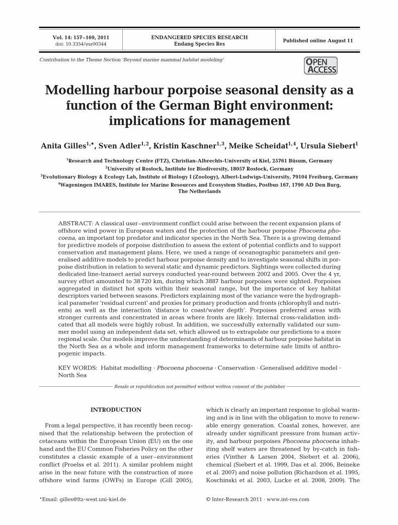
All spatial analyses were conducted at a resolutionof 10 × 10 km in ArcGIS 9.2 (ESRI). Porpoise sightingdata were extracted for each 10 km segment of on-effort transect. We selected this resolution to ensurethat sighting conditions and geographic location didnot change appreciably within this sampling unit(Hedley & Buckland 2004). We derived an estimateof porpoise density corrected for the detection pro -bability (see Gilles et al. 2009) and used these esti-mates as our response variable. Additionally, the sur-vey effort was included in the model formula as aweighting factor to prevent potential biases resultingfrom over- or undersampling sub-regions within eachblock.

Testing for seasonal differences. We carried out anexploratory analysis to determine potential significantseasonal shifts in porpoise distribution. We used a gen-eralised additive model (GAM) to model porpoise den-sity based on latitude and longitude following Wood(2006, p. 239) to test for the effect of season. At first,assuming no difference in spatial distribution through-out the year, all data were pooled. A second model wasapplied assuming differences in spatial distributionpatterns caused by season (using by variables in ‘mgcv

1.4-1.1’ in R v.2.8.1; Wood 2008). Both models werethen compared by their residual deviance (using theanova.gam function). If there was a significant differ-ence between both models, we concluded that therewas evidence against symmetry and that this effectwas due to the factor ‘season’. This approach was car-ried out for all seasons. Results indicated significantdifferences between all of the 3 seasons (all p < 0.001).Consequently, we developed 3 distinct seasonal habi-tat prediction models.

Explanatory variables. The explanatory variableswere selected based on a priori knowledge of factorsknown to indirectly determine harbour porpoise distri-bution by influencing patterns in prey occurrence. As itwas not possible to collect in situ oceanographic dataduring the aerial surveys, we compiled spatially refer-enced oceanographic and remotely sensed data fromdifferent oceanographic databases. All data sets wereprocessed in ArcGIS 9.2 to generate correspondinggridded environmental data at the selected resolutionof 10 × 10 km.

We used a combination of static and dynamic predic-tors to fit the models, as listed in Table 2 and discussedin detail in the following.

Static predictors: Distance to shore (DIST) was cal-culated in ArcGIS as the shortest distance betweenthe midpoint of each grid cell and the closest point onthe coastline. Water depth (DEPTH) data wereobtained from a digital bathymetric map set with aspatial resolution of 617 m. As DIST and DEPTH arecorrelated (R2 = 0.8, p < 0.05), these 2 variables wereincluded as an interaction term (DIST,DEPTH) in allmodels. We hypothesised that this interaction termcould be important to capture the complex topogra-phy of the German Bight, where there are a numberof offshore shallows (e.g. Amrum and Dogger Banks).Bottom slope (SL) was derived from the depth data byusing the Spatial Analyst extension (Surface Analyst -

Endang Species Res 14: 157–169, 2011160

Explanatory Abbreviation Unit Predictor Spring mean Summer mean Autumn meanvariable category (median) ± SD (median) ± SD (median) ± SD

Distance to shore DIST km Static 81.4 (65.6) ± 71.0 81.4 (65.6) ± 71.0 81.4 (65.6) ± 71.0Water depth DEPTH m Static 29.3 (33.0) ± 13.6 29.3 (33.0) ± 13.6 29.3 (33.0) ± 13.6Slope SL ° Static 0.05 (0.03) ± 0.05 0.05 (0.03) ± 0.05 0.05 (0.03) ± 0.05Sea surface salinity SAL PSU Dynamic 31.9 (33.3) ± 3.5 32.7 (33.4) ± 2.1 32.2 (32.5) ± 2.1Sea surface temperature SST °C Dynamic 9.2 (8.9) ± 0.8 17.3 (17.2) ± 0.9 15.1 (15.2) ± 0.6Residual current CURR m s–1 Dynamic 0.07 (0.07) ± 0.02 0.06 (0.06) ± 0.01 0.09 (0.09) ± 0.02Sea surface chlorophyll CHL mg m–3 Dynamic 5.4 (4.4) ± 3.6 6.1 (5.1) ± 4.5 4.3 (3.0) ± 3.8Chlorophyll range CHL_r mg m–3 Dynamic 9.4 (7.0) ± 8.0 10.2 (8.4) ± 8.0 11.2 (9.2) ± 8.6Silicate SI µmol l–1 Dynamic 8.8 (6.4) ± 6.3 1.7 (1.1) ± 1.3 5.5 (3.7) ± 4 .1Nitrogen NI µmol l–1 Dynamic 18.7 (12.7) ± 15.1 25.4 (20.8) ± 15.6 25.9 (16.5) ± 21.8

Table 2. Overview of explanatory variables used for harbour porpoise habitat modelling. Average values for predictors withinthe Exclusive Economic Zone and 12 nautical mile zone are shown. Abbreviations as used throughout the text. DIST,DEPTH

was included as an interaction term

Flight Track line No. of No. ofdays length (km) groups individuals

Spring 19 10081 1234 1470Summer 32 15511 1462 1900Autumn 25 13128 392 517

Total 76 38720 3088 3887

Table 1. Phocoena phocoena. Sighting data. Results of theline-transect aerial survey in the German Exclusive EconomicZone and 12 nautical mile zone. Effort summary per seasonand main survey results in good and moderate sighting con -ditions are shown. Each season was pooled over the years

2002 to 2005

slope) in ArcGIS. Although derived from the bathy -metry, the slope at a particular location is indepen-dent of its depth (here: R2 = –0.5).

Dynamic predictors: We compiled data on dynamicpredictors for spring, summer and autumn across all 4study years in order to capture the range of seasonaland inter-annual environmental variability. We stroveto match each survey day with corresponding data foreach dynamic predictor at the highest available resolu-tion so as to capture the environmental situation foreach flight day as accurately as possible. Variableswere subsequently pooled for each season and aver-aged across all years.

Sea surface temperature (SST) data were availableat a weekly resolution and were provided by the Ger-man Federal Maritime and Hydrographic Agency(BSH) and derived from satellite data (Becker & Pauly1996). In order to derive mean seasonal values, we pro-cessed a total of 16, 21 and 21 weekly composites forspring, summer and autumn, respectively.

Data on residual currents (CURR) were computed bythe operational circulation model ‘BSHcmod’ and pro-vided by the BSH with a spatial resolution of 1 n mileon a daily basis. The so-called residual currents definethe net transport of the water mass, i.e., the influenceof the tidal currents is eliminated by suitable averag-ing, here over 2 tidal periods (Dick et al. 2001).

Surface chlorophyll concentration (CHL) was ob -tained from the multispectral sensor Medium Resolu-tion Imaging Spectrometer (MERIS) onboard the Euro-pean Space Agency (ESA)’s ENVISAT satellite(Doerffer et al. 1999). We analysed satellite imagesusing the BEAM software (www.brockmann-consult.de/beam). Mean values of surface chlorophyll concen-tration were extracted in ArcGIS from GeoTIFF filesproduced in BEAM by selecting the suitable spatialand band subset (algal_2, chlorophyll absorption). As aproxy for fronts or upwelling zones, which are oftencharacterised by chlorophyll anomalies, we subse-quently derived ‘chlorophyll range’ (CHL_r) from thechlorophyll data; representing the difference betweenthe maximum and minimum pixel value within our10 × 10 km grid cells.

We processed data on sea surface salinity (SAL)and selected nutrients (silicic acid, SI; and total nitro-gen, NI) from in situ measurements taken at oceano-graphic stations provided by the International Coun-cil for the Exploration of the Seas (ICES) and theGerman Oceanographic Data Centre. We used thesepoint coverages of salinity and nutrient concentra-tions to create interpolated raster surfaces across thestudy area. For interpolation we used the ordinarykriging function in ArcGIS (Geostatistical Analyst).However, we were only able to calculate seasonalvalues of nutrient concentration for spring and

autumn 2004 and for summer 2002, as the samplingcoverage was insufficient in the other years to allowa robust interpolation by season.

Model selection. Using the GAM setup of ‘mgcv 1.4-1.1’ in R v.2.8.1 (R Development Core Team 2008), wemodelled the estimated probability of porpoise densityat any site as an additive function of the selected envir -onmental predictors using a logarithmic link and aquasi-likelihood error distribution to account foroverdispersion in the data.

Model selection by season was based on identify-ing which predictors had significant effects by usingbackward (stepwise) selection (Redfern et al. 2006)and by stepwise comparing models using ANOVA.The ‘mgcv’ package uses an automated generalisedcross-validation for model fitting (GCV score; Wood2008). We set the significance level to α = 0.1 inorder not to exclude important predictors, as thestudy area is very heterogeneous. However, this onlybecame an issue in spring when the model signifi-cantly improved when including CHL (Table 3), asshown by the ANOVA.

Model error for the best-fit models was determinedas the sum of squared residuals. However, modelselection may have been biased due to (1) residual spa-tial autocorrelation (SACor) violating the assumptionof independence of observations (Legendre 1993) and(2) multicollinearity (Zuur et al. 2010). To address pos-sible bias (1), we plotted a correlogram of the residualsand visually inspected for signs of SACor (Keitt et al.2002). In addition, we compared GAM performancewith a generalised additive mixed model (GAMM; e.g.Wood 2008), as this allows modelling of non-linearrelationships while explicitly taking SACor intoaccount. The SACor structure we used in the mixedeffect model (function gamm in ‘mgcv’) has an expo-nential structure and is implemented by the ‘corExp’functions of the ‘nlme’ package in R (Pinheiro & Bates2000). To deal with bias (2), we determined the vari-ance inflation factors (VIF) and set a stringent thresh-old of VIF = 3 as suggested by Zuur et al. (2010).

Assessment of model performance and validation.To assess model performance, we compared observedporpoise densities with predicted density surfaces. Thespatial distribution of the response residuals by gridcell was also mapped in order to identify areas wherethe model over- or underestimated density (i.e. residu-als were negative or positive, respectively).

Subdividing our study area into 9 spatial subsets ofequal size, we followed standard k-fold cross-valida-tion (Wood 2006, Schröder 2008) to validate the predic-tive accuracies of the resulting best-fit models usingwithheld subsets as test data by calculating the rootmean square error of prediction (RMSEP; Redfern et al.2008).

Gilles et al.: Modelling harbour porpoise density 161

Here, we carried out both internal and externalvalidations based on an enlarged study area (whitebox in Fig. 1), which encompassed a sufficientlylarge proportion of the area covered by the SCANS-II survey providing our independent data (seebelow). We performed internal validation of eachseason by using subsets of the original data and theexternal validation by using independent data to val-idate the summer model. The independent data werecollected during the SCANS-II survey, which esti-mated small cetacean abundance in the North Sea

and European Atlantic continental shelf waters inJuly 2005 (SCANS-II 2008). We used data of surveyblocks that overlapped with our study area (i.e.blocks H, L, U, V and Y; see SCANS-II 2008).

Estimation of abundance and variance. The finalselected models were parameterised in all grid cells togenerate a density surface over the whole study area.Abundance of animals in the SACs was predicted byintegrating under the density surface. The variance ofthe abundance estimates was generated using non-parametric bootstrap methods (10 000 replicates; Efron1990), where the models were re-fitted for each boot -strap iteration.

RESULTS

Model selection

In general, selected predictors varied between the 3seasons. The summer model explained the highestdeviance, followed by spring and autumn (Table 3).The interaction (DIST,DEPTH) was the predictor mostoften selected in all models, followed by residual cur-rent (CURR) and chlorophyll concentration (CHL). Assingle factors, nitrogen (NI) and CURR each explainedthe most deviance, which is indicated by the high asso-ciated F-value (Table 3). As a measure of goodness offit, we analysed diagnostic plots and spatial structureof residuals that indicated no autocorrelation of resi -duals. Further, the comparison between GAM andGAMM outputs indicated that model performance andpredictions were very similar. For all 3 seasons, scatterplots of GAM versus GAMM residuals showedunskewed distributions of residuals, indicating similarpredictive ability of both models. Similarly, the meanerror and the spatial distribution of the residuals werecomparable during all seasons for both approaches,although the GAMM in fact performed worse than theless complex GAM.

Observed and predicted distribution

In spring, observed harbour porpoise distributionwas highly heterogeneous (Fig. 2a). Porpoise densitywas highest in the north-east around the Sylt OuterReef (SOR, see Fig. 1) and about 60 km offshore of theEast Frisian Islands, in an area called Borkum ReefGround (BRG, see Fig. 1). Other high density areaswere found at the Dogger Tail End (Fig. 2a).

The modelled response surface (Fig. 2b) showed agood fit of the observed density distribution andcaptured the 2 hot spots in SOR and BRG very well. Thesmaller hot spot at the edge of the Dogger Bank was also

Endang Species Res 14: 157–169, 2011162

Explanatory GAMvariable Spring Summer Autumn

Intercept t –4.43 –8.45 –13.24Pr(>|t|) <0.001 <0.001 <0.001

Estimate –0.34 –0.74 –1.63

DIST,DEPTH F 4.72 3.90 3.55p <0.001 <0.001 <0.001

edf 21.6 10.25 18.8

SL F 3.56 NS NSp 0.01 NS NS

edf 3.01 NS NS

SST F 5.71 MC NSp <0.001 MC NS

edf 5.46 MC NS

SAL F MC NS 3.48p MC NS <0.001

edf MC NS 8.5

CURR F 10.07 3.35 NSp <0.001 0.002 NS

edf 1.0 6.22 NS

CHL F 1.81 NS 2.31p 0.09 NS 0.03

edf 5.87 NS 5.8

CHL_r F 3.79 NS 5.95p 0.03 NS 0.007

edf 1.11 NS 1

SI F MC NS NSp MC NS NS

edf MC NS NS

NI F NS 15.25 NSp NS <0.001 NS

edf NS 2.11 NS

n 389 419 388R2 adj. 0.45 0.56 0.40Deviance explained (%) 52.1 56.9 42.6Model error 1.23 1.09 0.47

Table 3. Best-fit model. F-values, significance test p-valuesand estimated degrees of freedom (edf) are given for the ex-planatory variables (for abbreviations, see Table 2). The ad-justed R2, deviance explained (%) and model error (sum ofsquared residuals) are also shown. Terms that were not signif-icant (NS, p > 0.1) were dropped from the model. MC: not in-cluded due to multicollinearity. GAM: generalised additive

model

predicted successfully. The model predicted increasingporpoise density, when moving from the island of He-ligoland north towards SOR and further north-west.

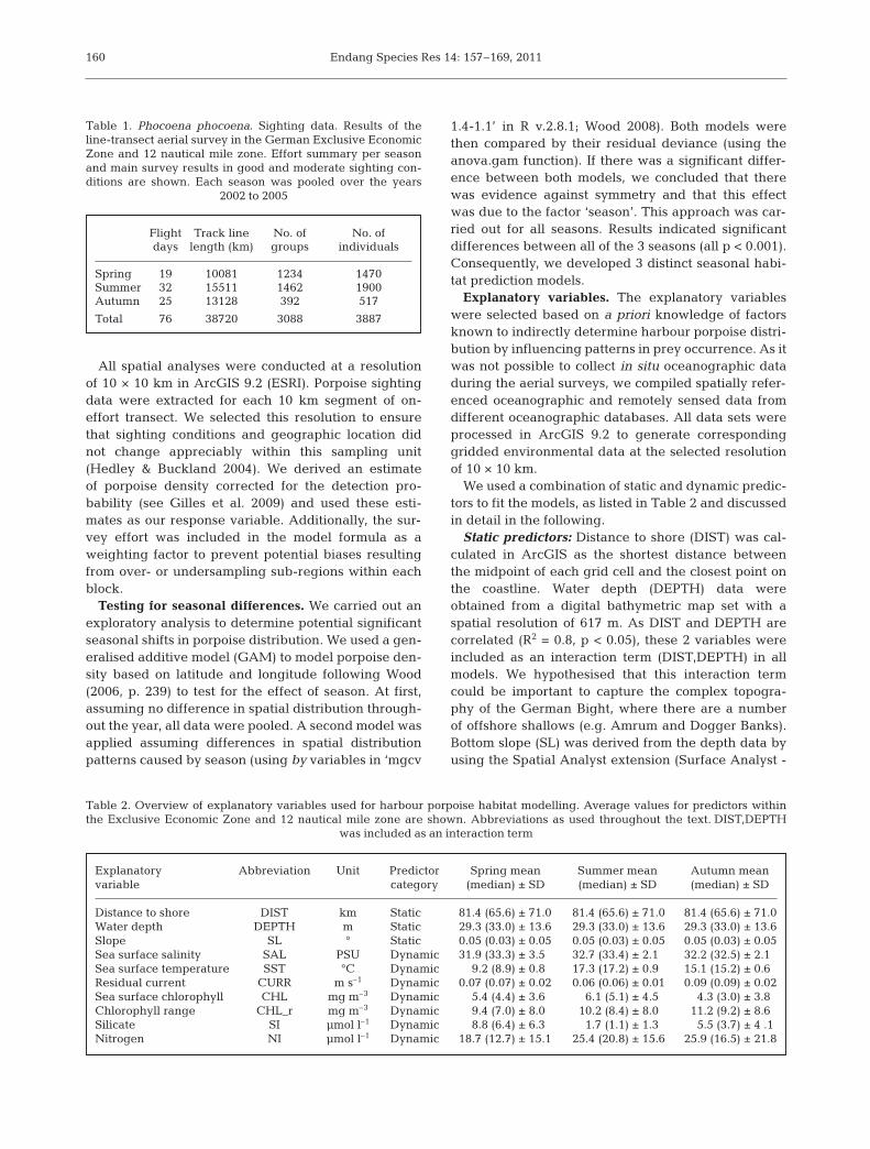
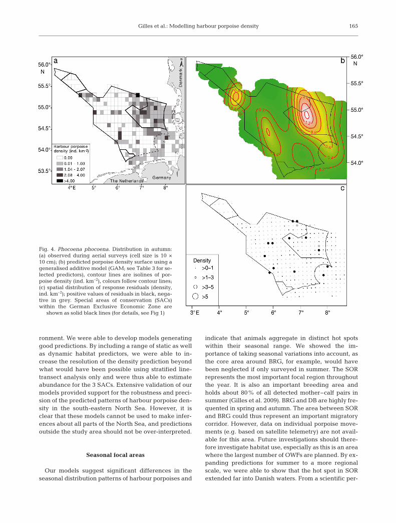
Maximum porpoise densities within our study areawere observed in the summer and were accompaniedby a substantial northward shift, resulting in a de -crease of densities in the southern German Bight andan increase in the North (Fig. 3a). The response surfaceshowed a very good fit with the observed spatial pat-tern (Fig. 3b). The aerial surveys in autumn revealedthat porpoises were more evenly dispersed throughoutthe study area and that they occurred at lower densi-ties in comparison to the other seasons (Fig. 4a). Thispattern was captured well by the model. The predicteddensity surface showed 2 focal areas, one again aroundthe reef structure of the SOR and another at the Dog-ger Tail End (Fig. 4b).

The spatial distribution of response residualsshowed that the GAM underestimated density in the

north-east and along the northern frontier of theEEZ in spring and summer (Figs. 2c & 3c), whereasin autumn residuals showed low values and no par-ticular area with extreme under- or overestimation(Fig. 4c).

Model validation

Internal and external cross-validation also providedsupport for a good fit for all 3 models, as indicated bylow RMSEPs. RMSEPs based on internal validationwere very similar between spring (RMSEP = 1.79) andsummer (RMSEP = 1.51) and lowest for autumn(RMSEP = 0.57). As RMSEPs are not standardised, thishas to be seen in the context of densities being lowestin autumn. The external validation with the indepen-dent data set SCANS-II focused on the transferabilityand generalisability of the summer model and resulted

Gilles et al.: Modelling harbour porpoise density 163

Fig. 2. Phocoena phocoena. Distribution in spring:(a) observed during aerial surveys (cell size is 10 ×10 cm); (b) predicted porpoise density surface using ageneralised additive model (GAM; see Table 3 for se-lected predictors), contour lines are isolines of por-poise density (ind. km–2), colours follow contour lines;(c) spatial distribution of response residuals (density,ind. km–2); positive values of residuals in black, nega-tive in grey. Special areas of conservation (SACs)within the German Exclusive Economic Zone are

shown as solid black lines (for details, see Fig. 1)

Endang Species Res 14: 157–169, 2011

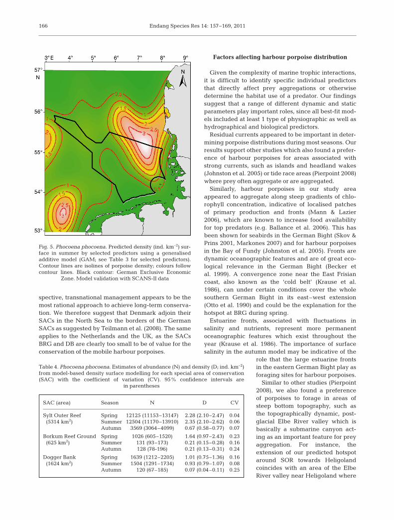
in a positive validation (RMSEP = 1.21). As a conse-quence, we used the GAM best-fit model, based on thelocal summer data, to predict porpoise density for amore regional scale as supported by the SCANS-II val-idation (Fig. 5). The results showed that the summerhot spot in the north-eastern German Bight was pre-dicted to extend far into Danish waters. Additionalhigh density areas were predicted offshore the WestFrisian Islands in the Netherlands, near the EasternChannel and on the Dogger Bank.

Model-based abundance estimates

The seasonal abundance estimates for the area of the3 SACs show highest estimates for SOR and DB insummer and for BRG in spring (Table 4). In general,confidence intervals are narrow and coefficients ofvariation are of low value.

DISCUSSION

As scientists advising conservation agencies andmanagers, we are frequently asked to provide infor-mation on distribution and abundance for specific ar-eas. Such requests are often the basis for marine spa-tial planning and the definition of anthropogenicimpact zones or for the establishment of significancethresholds for designated marine protected areas. Thesize of such areas of interest often means that this de-mand cannot be met by dedicated surveys alone, sincethese can only provide estimates for predefined sur-vey strata. Instead, density surfaces are needed; theserequire modelling and, in turn, an ultimate under-standing of the environmental factors which influenceseasonal distribution in order to predict changes. Thisis the first study to investigate Phocoena phocoenadistribution and density throughout the year as a func-tion of the complex and dynamic German Bight envi-

164

Fig. 3. Phocoena phocoena. Distribution in summer:(a) observed during aerial surveys (cell size is 10 ×10 cm); (b) predicted porpoise density surface using ageneralised additive model (GAM; see Table 3 for se-lected predictors), contour lines are isolines of por-poise density (ind. km–2), colours follow contour lines;(c) spatial distribution of response residuals (density,ind. km–2); positive values of residuals in black, nega-tive in grey. Special areas of conservation (SACs)within the German Exclusive Economic Zone areshown as solid black lines (for details, see Fig. 1)

Gilles et al.: Modelling harbour porpoise density 165

ronment. We were able to develop models generatinggood predictions. By including a range of static as wellas dynamic habitat predictors, we were able to in-crease the resolution of the density prediction beyondwhat would have been possible using stratified line-transect analysis only and were thus able to estimateabundance for the 3 SACs. Extensive validation of ourmodels provided support for the robustness and preci-sion of the predicted patterns of harbour porpoise den-sity in the south-eastern North Sea. However, it isclear that these models cannot be used to make infer-ences about all parts of the North Sea, and pre dictionsoutside the study area should not be over-interpreted.

Seasonal focal areas

Our models suggest significant differences in theseasonal distribution patterns of harbour porpoises and

indicate that animals aggregate in distinct hot spotswithin their seasonal range. We showed the im -portance of taking seasonal variations into account, asthe core area around BRG, for example, would havebeen neglected if only surveyed in summer. The SORrepresents the most important focal region throughoutthe year. It is also an important breeding area andholds about 80% of all detected mother–calf pairs insummer (Gilles et al. 2009). BRG and DB are highly fre-quented in spring and autumn. The area between SORand BRG could thus represent an important migratorycorridor. However, data on individual porpoise move-ments (e.g. based on satellite telemetry) are not avail-able for this area. Future investigations should there-fore investigate habitat use, especially as this is an areawhere the largest number of OWFs are planned. By ex-panding predictions for summer to a more regionalscale, we were able to show that the hot spot in SORextended far into Danish waters. From a scientific per-

Fig. 4. Phocoena phocoena. Distribution in autumn:(a) observed during aerial surveys (cell size is 10 ×10 cm); (b) predicted porpoise density surface using ageneralised additive model (GAM; see Table 3 for se-lected predictors), contour lines are isolines of por-poise density (ind. km–2), colours follow contour lines;(c) spatial distribution of response residuals (density,ind. km–2); positive values of residuals in black, nega-tive in grey. Special areas of conservation (SACs)within the German Exclusive Economic Zone are

shown as solid black lines (for details, see Fig 1)

spective, transnational management appears to be themost rational approach to achieve long-term conserva-tion. We therefore suggest that Denmark adjoin theirSACs in the North Sea to the borders of the GermanSACs as suggested by Teilmann et al. (2008). The sameapplies to the Netherlands and the UK, as the SACsBRG and DB are clearly too small to be of value for theconservation of the mobile harbour porpoises.

Factors affecting harbour porpoise distribution

Given the complexity of marine trophic interactions,it is difficult to identify specific individual predictorsthat directly affect prey aggregations or otherwisedetermine the habitat use of a predator. Our findingssuggest that a range of different dynamic and staticparameters play important roles, since all best-fit mod-els included at least 1 type of physiographic as well ashydrographical and biological predictors.

Residual currents appeared to be important in deter-mining porpoise distributions during most seasons. Ourresults support other studies which also found a prefer-ence of harbour porpoises for areas associated withstrong currents, such as islands and headland wakes(Johnston et al. 2005) or tide race areas (Pierpoint 2008)where prey often aggregate or are aggregated.

Similarly, harbour porpoises in our study areaappeared to aggregate along steep gradients of chlo -rophyll concentration, indicative of localised patchesof primary production and fronts (Mann & Lazier2006), which are known to increase food availabilityfor top predators (e.g. Ballance et al. 2006). This hasbeen shown for seabirds in the German Bight (Skov &Prins 2001, Markones 2007) and for harbour porpoisesin the Bay of Fundy (Johnston et al. 2005). Fronts aredynamic oceanographic features and are of great eco-logical relevance in the German Bight (Becker etal. 1999). A convergence zone near the East Frisiancoast, also known as the ‘cold belt’ (Krause et al.1986), can under certain conditions cover the wholesouthern German Bight in its east–west extension(Otto et al. 1990) and could be the explanation for thehotspot at BRG during spring.

Estuarine fronts, associated with fluctuations insalinity and nutrients, represent more permanentoceanographic features which exist throughout theyear (Krause et al. 1986). The importance of surfacesalinity in the autumn model may be indicative of the

role that the large estuarine frontsin the eastern German Bight play asforaging sites for harbour porpoises.

Similar to other studies (Pierpoint2008), we also found a preferenceof porpoises to forage in areas ofsteep bottom topography, such asthe topographically dynamic, post-glacial Elbe River valley which isbasically a submarine canyon act-ing as an important feature for preyaggregation. For instance, theextension of our predicted hotspotaround SOR towards Heligolandcoincides with an area of the ElbeRiver valley near Heligoland where

Endang Species Res 14: 157–169, 2011166

SAC (area) Season N D CV

Sylt Outer Reef Spring 12125 (11153–13147) 2.28 (2.10–2.47) 0.04(5314 km2) Summer 12504 (11170–13910) 2.35 (2.10–2.62) 0.06

Autumn 3569 (3064–4099) 0.67 (0.58–0.77) 0.07

Borkum Reef Ground Spring 1026 (605–1520) 1.64 (0.97–2.43) 0.23(625 km2) Summer 131 (93–173) 0.21 (0.15–0.28) 0.16

Autumn 128 (78-196) 0.21 (0.13–0.31) 0.24

Dogger Bank Spring 1639 (1212–2205) 1.01 (0.75–1.36) 0.16(1624 km2) Summer 1504 (1291–1734) 0.93 (0.79–1.07) 0.08

Autumn 120 (67–185) 0.07 (0.04–0.11) 0.25

Table 4. Phocoena phocoena. Estimates of abundance (N) and density (D; ind. km–2)from model-based density surface modelling for each special area of conservation(SAC) with the coefficient of variation (CV). 95% confidence intervals are

in parentheses

Fig. 5. Phocoena phocoena. Predicted density (ind. km–2) sur-face in summer by selected predictors using a generalised additive model (GAM; see Table 3 for selected predictors).Contour lines are isolines of porpoise density; colours followcontour lines. Black contour: German Exclusive Economic

Zone. Model validation with SCANS-II data

Gilles et al.: Modelling harbour porpoise density

ephemeral upwelling occurs when easterly winds pre-vail (Krause et al. 1986).

In addition to salinity and temperature, nutrient dataare a valuable tool to differentiate water masses andprovide information on the recent state of biogeochem-ical turnover processes (Ehrich et al. 2007). In our sum-mer model, total nitrogen concentration was the mostinfluential predictor, and porpoise densities were pre-dicted to be higher in areas where nitrogen concentra-tion was low. As the depletion of nutrients such asnitrogen may be indicative of preceding phytoplank-ton blooms, low nitrogen levels suggest the onset ofsecondary production. Porpoise aggregation in suchareas can be expected to occur with a certain time lagto allow for sufficient time for zooplankton abundanceto rise, fish to locate the area and top predators toarrive.

Model-based abundance estimates

Predictive cetacean-habitat modelling is very usefulin that the incorporation of oceanographic variabilitycan improve conventional abundance estimates byreducing the variance (Forney 2000, Gómez de Seguraet al. 2007) as also shown in the present study. In com-parison, conventional line-transect estimates for thesurvey block including SOR resulted in 2.41 ind. km–2

(95% CI: 1.37–4.75; CV = 0.33) in summer (Gilles et al.2009). Thus, model-based estimates provide a higherpotential to detect significant changes in local abun-dances. It is clearly of advantage that spatial modelsallow abundance estimation in any subset of the studyarea, but the robustness of such estimates depends onthe appropriateness and the validation of the fittedmodel. It must be applied with considerable caution,particularly if the sub-area is small relative to the mod-elled area (Hammond 2010). Unfortunately, there is notyet a rule of thumb to determine a ‘small’ area. Futurework should consider this issue in more detail. How-ever, we are aware that the SAC BRG in particular issmall in comparison to the hot spot predicted in spring,and this should be kept in mind when using these esti-mates in a management context.

CONCLUSION

Our models provide important new information inunderstanding the determinants of harbour porpoiseseasonal habitat in the North Sea. Further modellingexercises could include food competitors (such as harbour seals), concrete disturbance factors (e.g.anthropogenic noise) or effects of climate change (e.g.increase in water temperature or change in currents).

The study clearly showed that the influence of predic-tors varied between seasons, highlighting the impor-tance of taking seasonal variations into account in anymarine spatial planning exercise. The delimitation ofSACs in our area proved to be, in part, a good fit con-cerning core areas for Phocoena phocoena. The fullimpact of OWFs in terms of the user–environment con-flict cannot be quantified until further farms have beenbuilt; however, our models could then be used as valu-able tools to help managers address concerns aboutthe potential impact from human activities.

Acknowledgements. Aerial surveys were financed by theGerman Federal Ministry for the Environment, Nature Con-servation and Nuclear Safety (BMU; MINOS and MINOSplus,FKZ 0327520, 0329946B), Ministry of Food, Agriculture andConsumer Protection (BMELV; 514-33.29/03HS059) and theFederal Agency for Nature Conservation (BfN; EMSON, FKZ80285260). We thank all pilots, observers and navigators.Thanks also to F. Colijn and 2 anonymous reviewers for valu-able comments on the manuscript. We thank the GermanFederal Maritime and Hydrographic Agency (BSH), the Inter-national Council for the Exploration of the Seas (ICES) andthe GKSS Research Centre, Department of Operational Sys-tems, for providing the various data sets. We are grateful to G.Bruss for assistance with data on residual currents. Thanks toP. Hammond and all the people and institutions involved inSCANS-II.

LITERATURE CITED

Ballance LT, Pitman RL, Fiedler PC (2006) Oceanographicinfluences on seabirds and cetaceans of the eastern tropi-cal Pacific: a review. Prog Oceanogr 69:360–390

Becker GA, Pauly M (1996) Sea surface temperature changesin the North Sea and their causes. ICES J Mar Sci 53:887–898

Becker GA, Dick S, Dippner J (1992) Hydrography of the Ger-man Bight. Mar Ecol Prog Ser 91:9–18

Becker GA, Giese H, Isert K, König P, Langenberg H,Pohlmann T, Schrum C (1999) Mesoscale structures, fluxesand water mass variability in the German Bight as exem-plified in the KUSTOS-experiments and numerical mod-els. Ocean Dyn 51:155–179

Beineke A, Siebert U, Stott J, Müller G, Baumgärtner W(2007) Phenotypical characterization of changes in thymusand spleen associated with lymphoid depletion in free-ranging harbor porpoises (Phocoena phocoena). VetImmunol Immunopathol 117:254–265

Buckland ST, Anderson DR, Burnham KP, Laake JL, BorchersDL, Thomas L (2001) Introduction to distance sampling.Estimating abundance of biological populations. OxfordUniversity Press, New York, NY

Das K, Vossen A, Tolley K, Vikingsson GA and others (2006)Interfollicular fibrosis in the thyroid of the harbour por-poise: an endocrine disruption? Arch Environ ContamToxicol 51:720–729

Dick S, Kleine E, Müller-Navarra S, Klein H, Komo H (2001)The operational circulation model of BSH (BSHcmod) —model description and validation. Ber BSH no. 29. FederalMaritime and Hydrographic Agency (BSH), Hamburg

Doerffer R, Sorensen K, Aiken J (1999) MERIS potential forcoastal zone applications. Int J Remote Sens 20:1809–1818

167

Endang Species Res 14: 157–169, 2011168

Efron B (1990) More efficient bootstrap computations. J AmStat Assoc 85:79–89

Ehrich S, Adlerstein A, Brockmann U, Floeter U and others(2007) 20 years of German small-scale bottom trawl survey(GSBTS): a review. Senckenb Marit 37:13–82

Embling CB, Gillibrand PA, Gordon J, Shrimpton J, StevickPT, Hammond PS (2010) Using habitat models to identifysuitable sites for marine protected areas for harbour por-poises (Phocoena phocoena). Biol Conserv 143:267–279

Forney KA (2000) Environmental models of cetacean abun-dance: reducing uncertainty in population trends. ConservBiol 14:1271–1286

Gill AB (2005) Offshore renewable energy: ecological impli-cations of generating electricity in the coastal zone. J ApplEcol 42:605–615

Gilles A (2009) Characterisation of harbour porpoise (Pho-coena phocoena) habitat in German waters. PhD disserta-tion, University of Kiel

Gilles A, Scheidat M, Siebert U (2009) Seasonal distribution ofharbour porpoises and possible interference of offshorewind farms in the German North Sea. Mar Ecol Prog Ser383:295–307

Gómez de Segura A, Hammond PS, Cañadas A, Raga JA(2007) Comparing cetacean abundance estimates derivedfrom spatial models and design-based line transect meth-ods. Mar Ecol Prog Ser 329:289–299

Hammond PS (2010) Estimating the abundance of marinemammals. In: Boyd IL, Bowen WD, Iverson SJ (eds)Marine mammal ecology and conservation. Oxford Uni-versity Press, Oxford, p 42–67

Hammond PS, Berggren P, Benke H, Borchers DL and others(2002) Abundance of harbour porpoises and othercetaceans in the North Sea and adjacent waters. J ApplEcol 39:361–376

Hedley SL, Buckland ST (2004) Spatial models for line tran-sect sampling. J Agric Biol Environ Stat 9:181–199

Hiby AR (1999) The objective identification of duplicate sight-ings in aerial survey for porpoise. In: Garner GW, AmstrupSC, Laake JL, Manly BFJ, McDonald LL, Robertson DG(eds) Marine mammal survey and assessment methods.Balkema, Rotterdam, p 179–189

Hiby AR, Lovell P (1998) Using aircraft in tandem formation toestimate abundance of harbour porpoises. Biometrics 54:1280–1289

Johnston DW, Westgate AJ, Read AJ (2005) Effects of fine-scale oceanographic features on the distribution andmovements of harbour porpoises Phocoena phocoena inthe Bay of Fundy. Mar Ecol Prog Ser 295:279–293

Keitt T, Bjornstadt O, Dixon P, Citron-Pousty S (2002)Accounting for spatial pattern when modeling organism–environment interactions. Ecography 25:616–625

Koopman HN (1998) Topographical distribution of the blub-ber of harbor porpoises (Phocoena phocoena). J Mammal79:260–270

Koschinski S, Culik BM, Damsgaard Henriksen O, TregenzaN, Ellis GM, Jansen C, Kathe G (2003) Behavioural reac-tions of free-ranging porpoises and seals to the noise of asimulated 2 MW windpower generator. Mar Ecol Prog Ser265:263–273

Krause G, Budeus G, Gerdes D, Schaumann K, Hesse K (1986)Frontal systems in the German Bight and their physicaland biological effects. In: Nihoul J (ed) Marine interfacesecohydrodynamics. Elsevier, Amsterdam, p 119–140

Legendre P (1993) Spatial autocorrelation: trouble or new par-adigm? Ecology 74:1659–1673

Lucke K, Lepper PA, Blanchet MA, Siebert U (2008) Testingthe acoustic tolerance of harbour porpoise hearing for

impulsive sounds. Bioacoustics 17:329–331Lucke K, Siebert U, Lepper P, Blanchet MA (2009) Temporary

shift in masked hearing thresholds in a harbor porpoise(Phocoena phocoena) after exposure to seismic airgunstimuli. J Acoust Soc Am 125:4060–4070

MacLeod CD, Weir CR, Pierpoint C, Harland EJ (2007) Thehabitat preferences of marine mammals west of Scotland(UK). J Mar Biol Assoc UK 87:157–164

Mann K, Lazier J (2006) Dynamics of marine ecosytems. Bio-logical–physical interactions in the oceans. BlackwellPublishing, Malden, MA

Markones N (2007) Habitat selection of seabirds in a highlydynamic coastal sea: temporal variation and influence ofhydrographic features. PhD dissertation, University of Kiel

Marubini F, Gimona A, Evans PGH, Wright PJ, Pierce GJ(2009) Habitat preferences and interannual variability inoccurrence of the harbour porpoise Phocoena phocoenaoff northwest Scotland. Mar Ecol Prog Ser 381:297–310

Otto L, Zimmerman JTF, Furnes GK, Mork M, Saetre R,Becker G (1990) Review of the physical oceanography ofthe North Sea. Neth J Sea Res 26:161–238

Pierpoint C (2008) Harbour porpoise (Phocoena phocoena)foraging strategy at a high energy, near-shore site insouth-west Wales, UK. J Mar Biol Assoc UK 88:1167–1173

Pinheiro J, Bates D (2000) Mixed-effect models in S and S-plus. Springer, New York, NY

Proelss A, Krivickaite M, Gilles A, Herr H, Siebert U (2011)Protection of cetaceans in European waters — a case studyon bottom-set gillnet fisheries within marine protectedareas. Int J Mar Coast Law 26:5–45

R Development Core Team (2008) R: a language and environ-ment for statistical computing. R Foundation for StatisticalComputing, Vienna. www.R-project.org

Redfern JV, Ferguson MC, Becker EA, Hyrenbach KD andothers (2006) Techniques for cetacean–habitat modeling.Mar Ecol Prog Ser 310:271–295

Redfern JV, Barlow J, Ballance LT, Gerrodette T, Becker EA(2008) Absence of scale dependence in dolphin–habitatmodels for the eastern tropical Pacific Ocean. Mar EcolProg Ser 363:1–14

Richardson WJ, Greene CR, Malme C, Thomson D (1995)Marine mammals and noise. Academic Press, New York,NY

Santos MB, Pierce GJ (2003) The diet of harbour porpoise(Phocoena phocoena) in the Northeast Atlantic. OceanogrMar Biol Annu Rev 41:355–390

SCANS-II (2008) Small cetaceans in the European Atlanticand North Sea. Final report to the European Commissionunder project LIFE04NAT/GB/000245. Sea MammalResearch Unit, Gatty Marine Laboratory, University of StAndrews, St Andrews

Scheidat M, Gilles A, Siebert U (2006) Evaluating the distrib-ution and density of harbour porpoises (Phocoena pho-coena) in selected areas in German waters. In: von Nord-heim H, Boedeker D, Krause J (eds) Progress in marineconservation in Europe. Springer, Berlin, p 189–208

Scheidat M, Gilles A, Kock KH, Siebert U (2008) Harbour por-poise Phocoena phocoena abundance in the southwesternBaltic Sea. Endang Species Res 5:215–223

Schröder B (2008) Challenges of species distribution model-ing belowground. J Plant Nutr Soil Sci 171:325–337

Siebert U, Joiris C, Holsbeek L, Benke H, Failing K, Frese K,Petzinger E (1999) Potential relation between mercuryconcentrations and necropsy findings in cetaceans fromGerman waters of the North and Baltic Seas. Mar PollutBull 38:285–295

Siebert U, Gilles A, Lucke K, Ludwig M, Benke H, Kock KH,

Gilles et al.: Modelling harbour porpoise density 169

Scheidat M (2006) A decade of harbour porpoise occur-rence in German waters — analyses of aerial surveys, inci-dental sightings and strandings. J Sea Res 56:65–80

Skov H, Prins E (2001) Impact of estuarine fronts on the dis-persal of piscivorous birds in the German Bight. Mar EcolProg Ser 214:279–287

Skov H, Thomsen F (2008) Resolving fine-scale spatio-tempo-ral dynamics in the harbour porpoise Phocoena phocoena.Mar Ecol Prog Ser 373:173–186

Teilmann J, Sveegaard S, Dietz R, Petersen IK, Berggren P,Desportes G (2008) High density areas for harbour por-poises in Danish waters. National Environmental ResearchInstitute Tech Rep 657. National Environmental ResearchInstitute, University of Aarhus. Available at www.dmu.dk/Pub/FR657.pdf

Tougaard J, Carstensen J, Teilmann J, Skov H, Rasmussen P(2009) Pile driving zone of responsiveness extends beyond20 km for harbor porpoises (Phocoena phocoena (L.)).

J Acoust Soc Am 126:11–14Vinther M, Larsen F (2004) Updated estimates of harbour por-

poise (Phocoena phocoena) bycatch in the Danish NorthSea bottom-set gillnet fishery. J Cetacean Res Manag 6:19–24

Wilson B, Reid RJ, Grellier K, Thompson PM, Hammond PS(2004) Considering the temporal when managing the spa-tial: a population range expansion impacts protectedareas-based management for bottlenose dolphins. AnimConserv 7:331–338

Wood S (2006) Generalized additive models: an introductionwith R. Chapman & Hall/CRC, Boca Raton, FL

Wood S (2008) Fast stable direct fitting and smoothness selec-tion for generalized additive models. J R Stat Soc Ser BStat Methodol 70:495–518

Zuur AF, Ieno E, Elphick C (2010) A protocol for data explo-ration to avoid common statistical problems. Methods EcolEvol 1:3–14

Editorial responsibility: Daniel Palacios,Pacific Grove, California, USA

Submitted: December 1, 2010; Accepted: March 8, 2011Proofs received from author(s): July 8, 2011