Embed Size (px)
Citation preview

Modelling Forces Using Python Exploring alpha particle scattering due to gold Atoms and the motion of a satellite about Mars
Jack Parkinson
ABSTRACT
The plum pudding and nucleus ideas of an atom are modelled using python and compared; the findings agree with those experimentally verified by Ernest Rutherford. Additionally, the motion of a satellite around Mars whilst Mars is stationary is compared to when Mars is moving and the conclusion is that there is no difference in the motions other than a shift in velocity.

Introduction Many problems in physics involve differential equations that can be very difficult or simply impossible to solve analytically; these must, therefore, be solved using numerical methods. This report considers the trajectory of a satellite around Mars with varying initial conditions, and a comparison between two models of the atom, the plum pudding and nucleus models, using alpha particle scattering. The coupled differential equations that result from these scenarios are solved using scipy.integrate.odeint, which, given a function and an equation relating the variables involved, and a set of initial conditions to integrate over, can return a set of solutions for the components of position and velocity for the satellite or alpha particles.
Alpha Particle Scattering
Theory The plum pudding and nucleus models describe what an atom is composed of; the former describes an atom as a sphere of uniform positive charge interspersed with negative electrons, whereas the latter takes an atom to be largely empty space with a small, hard nucleus at the centre with all the positive charge. This difference gives rise to different predictions for the behaviour of charged particles close to an atom. If alpha particles of mass m=6.645x10-‐27 kg and charge q=+2e C are fired at gold atoms of radius rga=67.5x10-‐12 m, mass M=326.97x10-‐27 kg and charge Q=+79e, then the force on the alpha particle at a distance r from the centre of the gold atom for the nucleus model is:
This is also valid for the plum pudding model provided that r ≥ rga where rga is the radius of the gold atom. For r < rga the force is instead given by a slightly different equation accounting for the difference in charge distribution within the atom:
Thus we find the equations of motion of the alpha particles in the x and y directions to be:
These are the equations used by scipy.integrate.odeint, along with initial conditions, to find the solutions numerically.
F =1
4⇡✏0
r2(1)
F =1
4⇡✏0
Qqr
r3ga(2)
x =kQq
m
x
(x2 + y
2)3/2(3)
y =kQq
m
y
(x2 + y
2)3/2(4)
x =kQq
m
x
r
3ga
(5)
y =kQq
m
y
r3ga(6)
For the nucleus model and the plum pudding model when r ≥ rga.
For the plum pudding model when r < rga.
k =1
4⇡✏0 =8.854x10-‐12 C2N-‐1m-‐2
is the permittivity of free space.

Method To compare the two models of the atom we used python to simulate firing 5 MeV alpha particles at a plum pudding atom and an atom with a nucleus. The crucial difference in the models as far as the mathematics is concerned is changing the equation for the forces from (3) and (4) to (5) and (6) for the plum pudding model when r < rga, and this is what the code does. Additionally it was necessary to alter the potential energy for the plum pudding model when the alpha particle entered the gold atom although this was not achieved successfully; this would, however, leave the position and velocity solutions unaffected as the potential energy was calculated using this solutions–the only effect is that the total energy of the alpha particle ‘appears’ to increase though this is obviously not the case in reality. The program was set up to shoot alpha particles at these atoms horizontally in the positive x direction with a speed of 15.5x10⁶ ms-‐1 from various heights above and below the centre of the atom using a while loop to provide a broad range of trajectories to analyse and compare. All atoms were fired from from a horizontal displacement of x0=-‐10rga. The initial set-‐up is shown below:
For the plum pudding model, the initial height was varied from 2rga ≥ y ≥ -‐2rga and for the nucleus model from 50rgn ≥ y ≥ -‐50rgn where rgn=5.0x10-‐15 m is the radius of the gold nucleus. The initial horizontal speed mentioned above was calculated as shown on the diagram, where K0 is the initial kinetic energy.
Results and Discussion As can be seen by figures 2 and 3, the two models produce very different trajectories for the incident alpha particles. The plum pudding model causes almost no deflection at all for all heights, whereas the nucleus model causes large deflections for alpha particles that pass very close to the centre, with some
alpha particles deflected over 90 degrees. In both cases, the majority of particles continue in the same direction as expected.
Figure 1: Initial Set-‐Up for Alpha Scattering Experiments
Figure 3: Plum Pudding Model Trajectories Figure 2: Nucleus Model Trajectories
Plotting the deflection angle as a function of initial vertical displacement produces the graphs below. The vertical scales clearly show the disparity between the levels of deflection produced by the two different models. The most striking difference is that there is close to zero deflection for an alpha particle passing near the centre of a plum pudding atom, yet almost 180 degree deflection for an alpha particle at the same position within a nucleus model atom. The maximum deflection in the plum pudding model occurs at a displacement of ±67.5 nm (i.e. rga at the edges of the atom) and is only about 0.04 degrees compared to a complete 180 degrees deflection for an alpha particle that is directed directly at the nucleus of the other model.
A plot of the energy changes for a single trajectory of both models shows that, as aforementioned, the total energy of an alpha particle appears to deviate inside the atom for the plum pudding model; however this is merely an issue with the code and not a real physical deviation. The graph is plotting potential energy as U=kQq/r2 when for r < rga, it is actually U=kQq(3-‐(r2/rga2))/2rga which is slightly lower; were this equation implemented within the model then energy conservation would
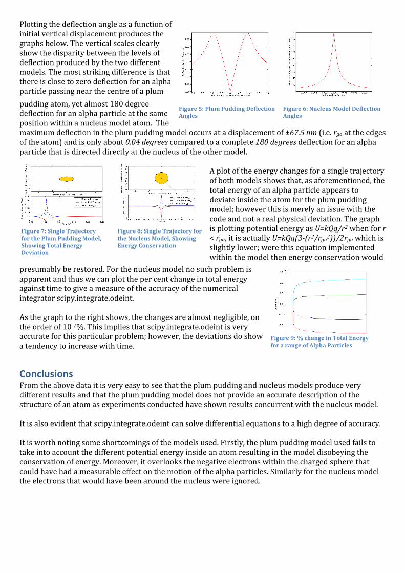
presumably be restored. For the nucleus model no such problem is apparent and thus we can plot the per cent change in total energy against time to give a measure of the accuracy of the numerical integrator scipy.integrate.odeint. As the graph to the right shows, the changes are almost negligible, on the order of 10-‐7%. This implies that scipy.integrate.odeint is very accurate for this particular problem; however, the deviations do show a tendency to increase with time.
Conclusions From the above data it is very easy to see that the plum pudding and nucleus models produce very different results and that the plum pudding model does not provide an accurate description of the structure of an atom as experiments conducted have shown results concurrent with the nucleus model. It is also evident that scipy.integrate.odeint can solve differential equations to a high degree of accuracy. It is worth noting some shortcomings of the models used. Firstly, the plum pudding model used fails to take into account the different potential energy inside an atom resulting in the model disobeying the conservation of energy. Moreover, it overlooks the negative electrons within the charged sphere that could have had a measurable effect on the motion of the alpha particles. Similarly for the nucleus model the electrons that would have been around the nucleus were ignored.
Figure 5: Plum Pudding Deflection Angles
Figure 6: Nucleus Model Deflection Angles
Figure 7: Single Trajectory for the Plum Pudding Model, Showing Total Energy Deviation
Figure 8: Single Trajectory for the Nucleus Model, Showing Energy Conservation
Figure 9: % change in Total Energy for a range of Alpha Particles
Motion of a Satellite About Mars
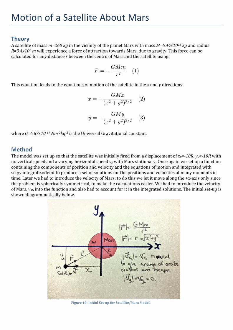
Theory A satellite of mass m=260 kg in the vicinity of the planet Mars with mass M=6.44x10²³ kg and radius R=3.4x10⁶ m will experience a force of attraction towards Mars, due to gravity. This force can be calculated for any distance r between the centre of Mars and the satellite using:
This equation leads to the equations of motion of the satellite in the x and y directions:
where G=6.67x10-‐11 Nm-‐2kg-‐2 is the Universal Gravitational constant.
Method The model was set up so that the satellite was initially fired from a displacement of x0=-‐10R, y0=-‐10R with no vertical speed and a varying horizontal speed vx with Mars stationary. Once again we set up a function containing the components of position and velocity and the equations of motion and integrated with scipy.integrate.odeint to produce a set of solutions for the positions and velocities at many moments in time. Later we had to introduce the velocity of Mars; to do this we let it move along the +x-‐axis only since the problem is spherically symmetrical, to make the calculations easier. We had to introduce the velocity of Mars, vM, into the function and also had to account for it in the integrated solutions. The initial set-‐up is shown diagrammatically below.
F = �GMm
r2(1)
x = � GMx
(x2 + y
2)3/2(2)
y = � GMy
(x2 + y
2)3/2(3)
Figure 10: Initial Set-‐up for Satellite/Mars Model.
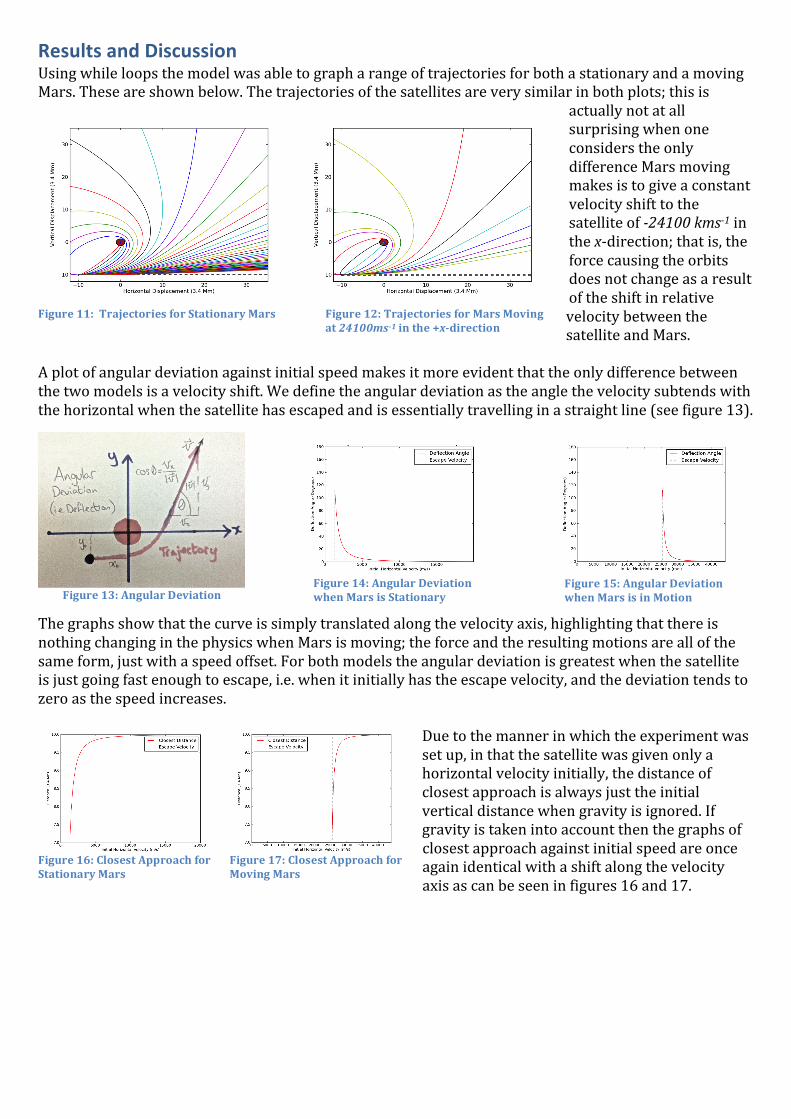
Results and Discussion Using while loops the model was able to graph a range of trajectories for both a stationary and a moving Mars. These are shown below. The trajectories of the satellites are very similar in both plots; this is
actually not at all surprising when one considers the only difference Mars moving makes is to give a constant velocity shift to the satellite of -‐24100 kms-‐1 in the x-‐direction; that is, the force causing the orbits does not change as a result of the shift in relative velocity between the satellite and Mars.
A plot of angular deviation against initial speed makes it more evident that the only difference between the two models is a velocity shift. We define the angular deviation as the angle the velocity subtends with the horizontal when the satellite has escaped and is essentially travelling in a straight line (see figure 13).
The graphs show that the curve is simply translated along the velocity axis, highlighting that there is nothing changing in the physics when Mars is moving; the force and the resulting motions are all of the same form, just with a speed offset. For both models the angular deviation is greatest when the satellite is just going fast enough to escape, i.e. when it initially has the escape velocity, and the deviation tends to zero as the speed increases.
Due to the manner in which the experiment was set up, in that the satellite was given only a horizontal velocity initially, the distance of closest approach is always just the initial vertical distance when gravity is ignored. If gravity is taken into account then the graphs of closest approach against initial speed are once again identical with a shift along the velocity axis as can be seen in figures 16 and 17.
Figure 11: Trajectories for Stationary Mars Figure 12: Trajectories for Mars Moving at 24100ms-‐1 in the +x-‐direction
Figure 13: Angular Deviation Figure 14: Angular Deviation when Mars is Stationary
Figure 15: Angular Deviation when Mars is in Motion
Figure 16: Closest Approach for Stationary Mars
Figure 17: Closest Approach for Moving Mars
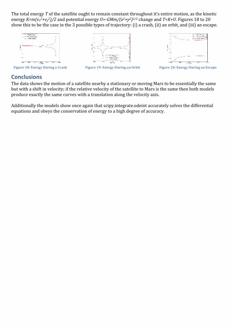
The total energy T of the satellite ought to remain constant throughout it’s entire motion, as the kinetic energy K=m(vx2+vy2)/2 and potential energy U=-‐GMm/(x2+y2)1/2 change and T=K+U. Figures 18 to 20 show this to be the case in the 3 possible types of trajectory: (i) a crash, (ii) an orbit, and (iii) an escape.
Conclusions The data shows the motion of a satellite nearby a stationary or moving Mars to be essentially the same but with a shift in velocity; if the relative velocity of the satellite to Mars is the same then both models produce exactly the same curves with a translation along the velocity axis. Additionally the models show once again that scipy.integrate.odeint accurately solves the differential equations and obeys the conservation of energy to a high degree of accuracy.
Figure 19: Energy During an Orbit Figure 20: Energy During an Escape Figure 18: Energy During a Crash