Modelling Fish Habitat Preference with a Genetic Algorithm ... · Modelling Fish Habitat Preference with a Genetic Algorithm-Optimized Takagi-Sugeno Model Based on Pairwise Comparisons

Modelling Fish Habitat Preference with a Genetic Algorithm-Optimized Takagi-Sugeno Model Based on Pairwise Comparisons

Shinji Fukuda, W illem W aegeman, Ans M outon, and Bernard D e Baets

A b strac t. Species-environm ent relationships are used for evaluating the current status o f target species and the potential im pact o f natural or anthropogenic changes of their habitat. Recent researches reported that the results are strongly affected by the quality of a data set used. The present study attem pted to apply pairw ise com parisons to m odelling fish habitat preference with Takagi-Sugeno-type fuzzy habitat preference models (FHPM s) optim ized by a genetic algorithm (GA). The model was com pared with the result obtained from the FF1PM optim ized based on mean squared error (M SE). Three independent data sets were used for training and testing of these models. The FFlPMs based on pairw ise com parison produced variable habitat preference curves from 20 different initial conditions in the GA. This could be partially ascribed to the optim ization process and the regulations assigned. This case study dem onstrates applicability and limitations of pairw ise com parison-based optim ization in an FF1PM. Future research should focus on a more flexible learning process to make a good use of the advantages of pairw ise comparisons.

1 Introduction

Ecological models are abstractions of natural systems and tools for understanding com plex processes and mechanism s involved. Flabitat preference models are

Shinji FukudaKyushu University, 6-10-1 Hakozaki, Fukuoka 812-8581, Japan e-mail: shinj i- fkd@agr . kyushu-u . ae . jpWillem Waegeman • Bernard De BaetsGhent University, Couple links 653, 9000 Ghent, Belgiume-mail: {Willem .Waegeman, Bernard. DeBaets} @ugent .beAns MoutonResearch Institute for Nature and Forest (INBO), Kliniekstraat 25, 1070 Brussels, Belgium e-mail: Ans .Mouton@inbo .be

B. De Baets et al. (Eds.): Eurofuse 2011, AISC 107, pp. 375-387, 2011. springerlink.com © Springer-Verlag Berlin Heidelberg 2011

376 S. Fukuda et al.

used in order to extract habitat preference inform ation of a target species from observation data, or to express expert knowledge on the species. Species-environm ent relationships can thus be quantified and used in the decision m aking on plans and m anagem ent options for a target ecosystem. In practice, there are two types of habitat models: univariate and m ultivariate models. Univariate models have been widely applied, for which the main idea consists o f using a set of univariate preference functions to represent possible habitat preference of a target species. These models are used for the assessm ent of current status and future impacts of habitat changes in both time and space [3], A variety of m ethods has been proposed and em ployed in practical applications, which include the habitat suitability index [3], resource selection functions [12], and other specific models such as a genetic Takagi-Sugeno fuzzy model [6 ,10], In recent years, multivariate approaches have gained m ore popularity as com putational systems have becom e powerful and freely available. These include m achine learning m ethods [14], fuzzy rule-based systems [1 ,16], and statistical regression tools [2, 9], In habitat modelling, it is often reported that the results are affected by the quality and quantity o f a data set used [5, 13], which is partly b ecause of the uncertainties inherent to observation data. The developm ent o f a sound m ethodology to cope with the different quality of data contributes to a better understanding and reliable assessm ent o f target ecosystems.

Preference modelling has been one of the key topics in inform ation sciences. Preference is used for ranking items and the ranking can be used for decision m aking. Recently, pairw ise com parison has been gaining interest in this field, and is reported to be a sound m ethodology in preference learning [7, 11], D espite the in tensive works in theory, the pairw ise com parison has not yet been applied to preference m odelling in ecology, and it seems to be a good approach to cope with the data with uncertainties such as observation errors. It would therefore be interesting to exem plify the applicability and lim itations of a pairw ise com parison-based approach.

Our aim is to apply pairw ise com parisons to the optim ization of a Takagi-Sugeno- type fuzzy habitat preference model (FHPM ) using a genetic algorithm (GA [8]). The results were com pared with the previously developed FHPM optim ized based on m ean squared error (M SE). Three independent data sets were used for training and testing of the models. This first application of pairw ise com parison provides useful inform ation for the developm ent of a reliable habitat assessm ent approach using observation data with uncertainty.

2 Methods

2.1 Data Collection

A series of field surveys focusing on Japanese m edaka ( O ryziasla tipes) was carried out in an agricultural canal in Kurum e City, Fukuoka, Japan. Field surveys were conducted on three sunny days: 14 October and 5 and 9 N ovem ber 2004. Two

Pairwise Comparisons for Modelling Fish Habitat Preference 377

study reaches were established in the same canal: a 50-m-long study reach (1 .6-2 .0 m in width, 0.3% gradient) was surveyed on 14 October and 5 November, and a 30-m -long study reach (0 .8-1 .4 m in width, 0.3% gradient) was surveyed on 9 November. Habitat use by Japanese m edaka and four physical habitat characteristics— water depth (cm, henceforth referred to as depth), current velocity (cm s_1, velocity), lateral cover ratio (%, cover), and percent vegetation coverage (%, vegetation)— in the study reach were surveyed. The study reach was first m apped, then habitat use by the fish was observed, and finally the physical habitat characteristics within the reach were measured.

In the following analyses, fish distribution data are expressed as the log- transform ed observed fish population density in the 1th water unit (F P D 0 individuals per square metre), where the subscript o indicates observed, i = 1, 2, ..., N, denotes the water unit, and N is the total num ber of water units (Table 1). The size of data sets (=N) is 139 for the data set of 14 October, 130 for that of 5 November, and 86 for that of 9 November, all o f which contain vectors of four habitat variables (depth, velocity, cover and vegetation) and fish population density.

Table 1 Species distribution data along with the four habitat variables of depth, velocity, cover and vegetation, each of which was observed on 14 October, 5 November, and 9 November 2004, respectively.

Date D Y C V EG logio(FPD-lT) presence absence prevalencemaximum 65.0 61.3 50.0 100.0 1.64

14 Oct. mean 13.6 13.7 19.1 49.7 0.37 77 62 55.4minimum 2.0 1.5 0.0 0.0 0.00

SD 8.0 9.3 14.0 29.6 0.41maximum 57.0 31.6 50.0 100.0 1.56

5 Nov. mean 13.6 8.8 20.6 59.5 0.35 71 59 54.6minimum 3.0 1.5 0.0 0.0 0.00

SD 8.4 5.6 14.8 31.2 0.40maximum 32.0 44.7 50.0 100.0 1.88

9 Nov. mean 15.6 12.5 19.8 55.2 0.42 31 55 36.0minimum 5.0 1.5 0.0 0.0 0.00

SD 6.2 9.6 13.9 33.3 0.60SD, standard deviation; D, depth (cm); V, velocity (cm s_1 ); C. cover ( % ) :

VEG, vegetation ( % ) ;

FPD, observed fish population density (individuals per square metre).

2.2 Fuzzy Habitat Preference Model

A fuzzy habitat preference model (FHPM [10]) was em ployed for describing the habitat preference of the target fish. An FHPM is a 0-order Takagi-Sugeno model [15] that relates habitat variables to habitat preference by considering uncertainties such as fish behaviour and m easurem ent errors o f the habitat variables.


Simultaneous optim ization of all model param eters enables an FHPM to evaluate habitat preference in an interpretable way, despite the presence of nonlinear, com plex interactions between habitat variables and habitat preference.

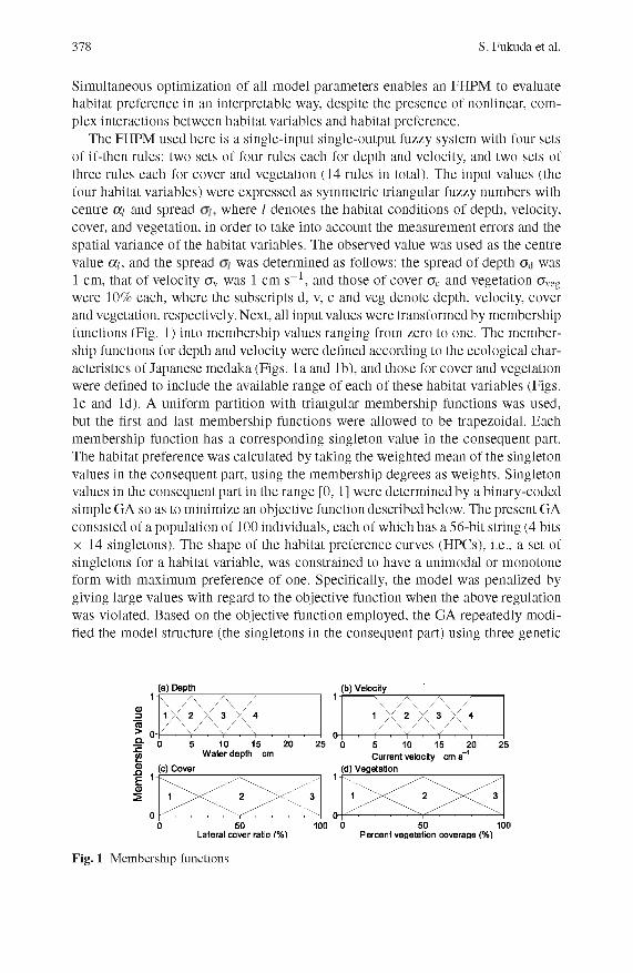
The FHPM used here is a single-input single-output fuzzy system with four sets o f if-then rules: two sets o f four rules each for depth and velocity, and two sets of three rules each for cover and vegetation (14 rules in total). The input values (the four habitat variables) were expressed as symm etric triangular fuzzy num bers with centre a¡ and spread where I denotes the habitat conditions of depth, velocity, cover, and vegetation, in order to take into account the m easurem ent errors and the spatial variance of the habitat variables. The observed value was used as the centre value a¡, and the spread was determ ined as follows: the spread of depth Gd was 1 cm, that o f velocity crv was 1 cm s_1, and those of cover crc and vegetation (7veg were 10% each, where the subscripts d, v, c and veg denote depth, velocity, cover and vegetation, respectively. Next, all input values w ere transform ed by membership functions (Fig. 1) into m em bership values ranging from zero to one. The m em bership functions for depth and velocity were defined according to the ecological characteristics of Japanese m edaka (Figs. la and lb ), and those for cover and vegetation were defined to include the available range of each of these habitat variables (Figs. le and Id). A uniform partition with triangular m em bership functions was used, but the first and last m em bership functions were allowed to be trapezoidal. Each mem bership function has a corresponding singleton value in the consequent part. The habitat preference was calculated by taking the w eighted m ean of the singleton values in the consequent part, using the m em bership degrees as weights. Singleton values in the consequent part in the range [0, 1] were determ ined by a binary-coded sim ple GA so as to minim ize an objective function described below. The present GA consisted of a population of 100 individuals, each of which has a 56-bit string (4 bits X 14 singletons). The shape of the habitat preference curves (HPCs), i.e., a set of singletons for a habitat variable, was constrained to have a unim odal or m onotone form with m axim um preference of one. Specifically, the model was penalized by giving large values with regard to the objective function when the above regulation was violated. Based on the objective function em ployed, the GA repeatedly m odified the model structure (the singletons in the consequent part) using three genetic

(a) Depth (b) V e loc ity

0 3>Q . 25 0 5 10 15

C urren t ve loc ity cm s-120 25

W a ter depth cm

(c) Cover

100Late ra l cover ratio (% ) P ercen t vege tation coverage (% )

Fig. 1 Membership functions


operations: roulette wheel selection with an elitist strategy, uniform crossover and m utation at a probability o f 5%. The optim al model was obtained after 2,000 iterations. The GA optim ization was repeated using 20 different sets o f initial conditions in order to evaluate the variablity of the model structure that resulted from the initial conditions.

2.3 Objective Function

We em ployed either o f mean squared error (M SE) between observed and predicted fish population density or mean penalty (MP) evaluated from pairw ise com parison as our objective function. The procedures to calculate each objective function are as follows.

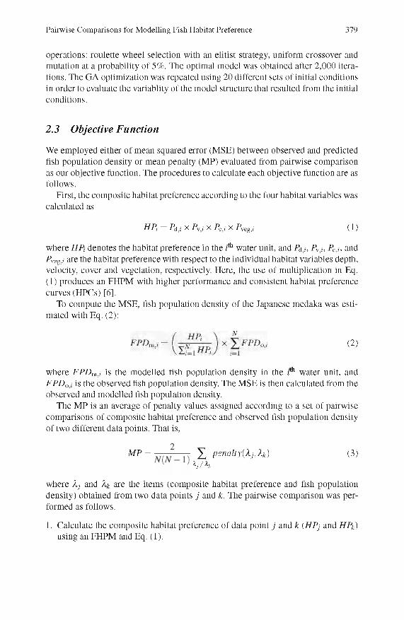
First, the com posite habitat preference according to the four habitat variables was calculated as

where HP, denotes the habitat preference in the 1th water unit, and P^„ Pv,i, Pc¡,, and PVeg,i are the habitat preference with respect to the individual habitat variables depth, velocity, cover and vegetation, respectively. Here, the use of multiplication in Eq. ( 1 ) produces an FHPM with higher perform ance and consistent habitat preference curves (HPCs) [6],

To com pute the M SE, fish population density of the Japanese m edaka was estimated with Eq. (2):

where F P D m¡, is the m odelled fish population density in the 1th water unit, and F P D 0 j is the observed fish population density. The M SE is then calculated from the observed and m odelled fish population density.

The M P is an average of penalty values assigned according to a set o f pairw ise com parisons of com posite habitat preference and observed fish population density of two different data points. That is,

where Xj and Xu are the items (com posite habitat preference and fish population density) obtained from two data points j and k. The pairw ise com parison was perform ed as follows.

HPj — P¿j X PV , X P: j X P y e g , i (1)

(2 )

M P = ^ h p ma ', y a 'M (3)

1. Calculate the com posite habitat preference of data point j and k (HPj and HPk) using an FHPM and Eq. (1).


2. For each of data points j and k,

2.1 Com pare the habitat preference values (HPj and HPk), from which either o f the relationships HPj > HP'k, HPj = HPk, or HPj < HPk is obtained.

2.2 Com pare the observed fish population density (FPD0j and FPDok), from which either o f the relationships FPD0j > FPDok, FPD0j = FPDok, or FPD0j < FPDo k is obtained.

2.3 Assign a penalty based on the relationship obtained from 2.1 and 2.2.a. If the relationships are the same between the habitat preference and fish

population density, then no penalty is assigned.

b. If the relationships are the opposite between the habitat preference and fish population density, then assign a penalty of 1.

c. If either o f the relationships is equal and the absolute difference of other relationship is smaller than a predefined value1, then assign a penalty of 0.5. O therwise, assign a penalty of 1.

3. Com pute the M P by means of Eq. (3).

2.4 Model Application and Analyses

To illustrate the difference between the FHPM s obtained from two different objective functions, these models were com pared in terms of model perform ance and habitat preference inform ation retrieved from them. The first data set was used for model developm ent (training), and the rem aining two data sets were used for model evaluation (testing). That is, 20 FHPM s were developed from each data set, each of which was tested using the other two different data sets. From the 20 initial conditions used in the model development, the variance of the model structures was quantified by using perform ance measures and the HPCs. The model perform ance was evaluated by the M SE, the M P and the area under receiver operating characteristics curve (AUC). The AUC is often used when evaluating species distribution models for presence-absence data [6, 14] and it is independent of the objective functions in this study. The M SE and M P were calculated using the fish population density and the AUC was calculated using the presence-absence data obtained from the fish population density data. O f these perform ance measures, the m ean and standard deviations of the 20 FHPM s from different initial conditions were used as a m easure of the predictive accuracy and of the variability o f model structures, respectively. In an FHPM , an HPC can easily be obtained by providing consecutive values in the range of the corresponding m em bership functions (in steps of 0.1 ) to the FHPM and plotting the output values against the habitat variables. Specifically, the HPC shape indicates the habitat preference inform ation retrieved from the data set used.

1 Allowed absolute difference for fish population density was set at 0.1 and that for habitat preference was at 0.05 (about 5% of then entire range).


3 Results

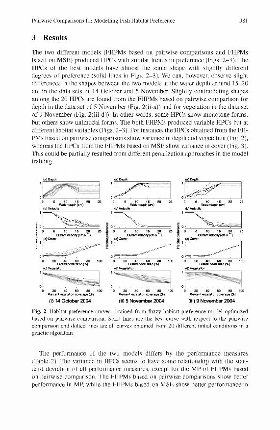
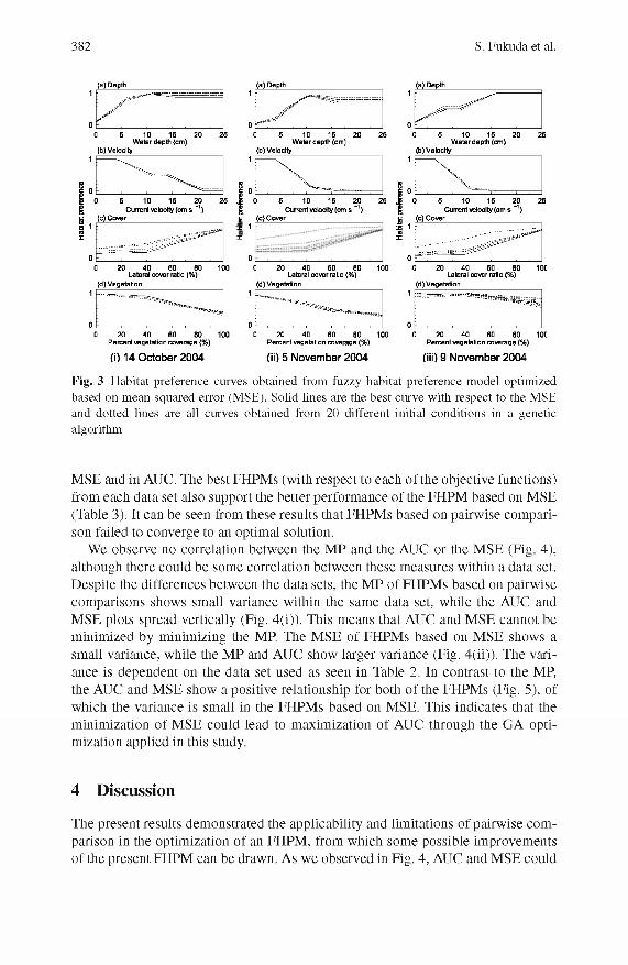
The two different models (FHPM s based on pairw ise com parisons and FHPM s based on M SE) produced HPCs with similar trends in preference (Figs. 2 -3 ). The HPCs of the best models have alm ost the same shape with slightly different degrees of preference (solid lines in Figs. 2 -3 ). We can, however, observe slight differences in the shapes between the two models at the water depth around 15-20 cm in the data sets o f 14 October and 5 November. Slightly contradicting shapes among the 20 HPCs are found from the FHPM s based on pairw ise com parison for depth in the data set o f 5 N ovem ber (Fig. 2(ii-a)) and for vegetation in the data set o f 9 N ovem ber (Fig. 2(iii-d)). In other words, some HPCs show m onotone forms, but others show unim odal forms. The both FHPM s produced variable HPCs but at different habitat variables (Figs. 2 -3 ). For instance, the HPCs obtained from the FH PMs based on pairw ise com parisons show variance in depth and vegetation (Fig. 2), whereas the HPCs from the FHPM s based on M SE show variance in cover (Fig. 3). This could be partially resulted from different penalization approaches in the model training.

(a) Depth (a) Depth (a) Depth

0P0 5 10 15 2 0 2 5

W ater depth (cm)(b) Velocity

0 5 10 15 2 0 2 5W ater depth (cm)

(b) Velocity

0 5 10 15 2 0 25W ater depth (cm)

(b) Velocity

0 5 10 15 20 25C u re n t velocity (cm s - l )

(c) C over

Lateral cover ratio (%) (d) V egetation



2 5 10 15 2 0Current velocity (cm s ~1)Current velocity (cm s "1)

(c) C over g (c) Cover !5 1 :raI

0100 0 20 40 60 80 100

■■ ............. 1

........................ :i!”j o 0P ercent vegetation coverage (%)

(il 14 O ctober 2004Percent vegetation c o re rag e (%)

(iii 5 Novem ber 2004Percent vegetation coverage (%)

(iii) 9 Novem ber 2004

Fig. 2 Habitat preference curves obtained from fuzzy habitat preference model optimized based on pairwise comparison. Solid lines are the best curve with respect to the pairwise comparison and dotted lines are all curves obtained from 20 different initial conditions in a genetic algorithm

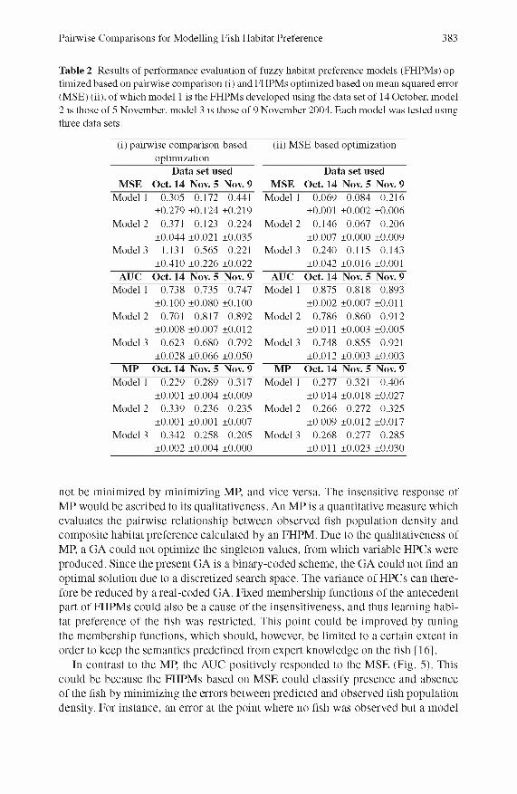
The perform ance of the two models differs by the perform ance measures (Table 2). The variance in HPCs seems to have some relationship with the standard deviation of all perform ance measures, except for the M P of FHPM s based on pairw ise com parison. The FHPM s based on pairw ise com parisons show better perform ance in MP, while the FHPM s based on M SE show better perform ance in


(a) Depth

0 5 10 15 2 0 25W ater depth (cm)

(b) Velocity

5 10 15 2 0 25Current velocity (cm s *1)

0 2 0 40 60 8 0 100Lateral cover ratio (%)

(d) V egetation

0 20 40 60 8 0 100Percent vegetation coverage {%)

iii 14 O ctober 2004

(a) Depth

0 5 10 15 2 0 25W ater depth (cm)

(b) Velocity

5 10 15 20 25C u re n t velocity (cm s ~1)

^ (c) Covers 1i

00 2 0 40 60 8 0 100

Lateral cover ratio (%)(d) V egetation

0 20 40 60 8 0 100Percent vegetation c overage (%)

Oil 5 November 2004

(a) Depth

0 5 10 15 2 0 2 5W ater depth (cm)

(b) Velocity

Current velocity (cm s “ )

0 2 0 40 60 8 0 10CLateral cover ratio (%)

(d) V egetation

0 20 40 60 8 0 10CPercent vegetation coverage (%)

(iii) 9 Novem ber 2004

Fig. 3 Flabitat preference curves obtained from fuzzy habitat preference model optimized based on mean squared error (MSE). Solid lines are the best curve with respect to the MSE and dotted lines are all curves obtained from 20 different initial conditions in a genetic algorithm

M SE and in AUC. The best FHPM s (with respect to each of the objective functions) from each data set also support the better perform ance of the FHPM based on M SE (Table 3). It can be seen from these results that FHPM s based on pairw ise com parison failed to converge to an optim al solution.

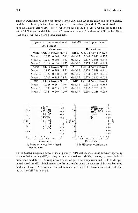
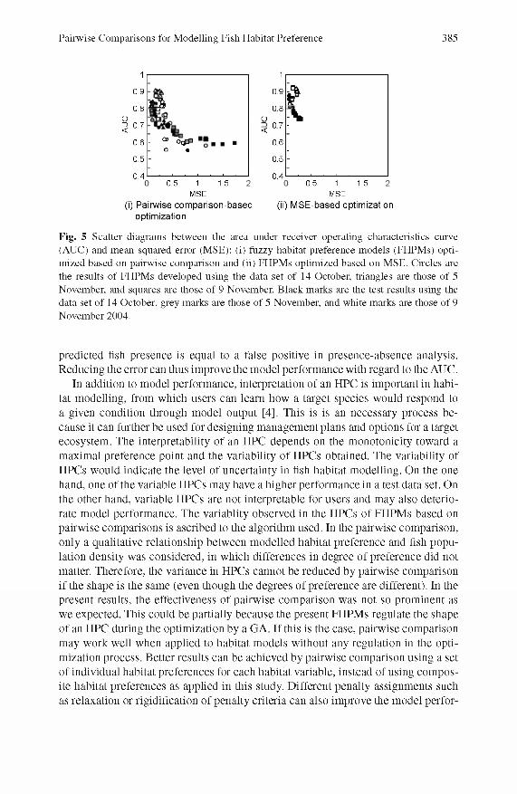
We observe no correlation between the M P and the AUC or the M SE (Fig. 4), although there could be some correlation between these m easures within a data set. D espite the differences between the data sets, the M P of FHPM s based on pairw ise com parisons shows small variance within the same data set, while the AUC and M SE plots spread vertically (Fig. 4(i)). This means that AUC and M SE cannot be m inim ized by minim izing the MP. The M SE of FHPM s based on M SE shows a small variance, while the M P and AUC show larger variance (Fig. 4(ii)). The variance is dependent on the data set used as seen in Table 2. In contrast to the MP, the AUC and M SE show a positive relationship for both of the FHPM s (Fig. 5), of which the variance is small in the FHPM s based on M SE. This indicates that the m inim ization of M SE could lead to maxim ization of AUC through the GA optimization applied in this study.

4 Discussion

The present results dem onstrated the applicability and lim itations of pairw ise com parison in the optim ization of an FHPM , from which some possible improvements o f the present FHPM can be drawn. As we observed in Fig. 4, AUC and M SE could


Table 2 Results of performance evaluation of fuzzy habitat preference models (FHPMs) optimized based on pairwise comparison (i) and FHPMs optimized based on mean squared error (MSE) (ii), of which model 1 is the FHPMs developed using the data set of 14 October, model 2 is those of 5 November, model 3 is those of 9 November 2004. Each model was tested using three data sets.

(i) pairwise comparison-based optimization

Data set usedMSE Oct. 14 Nov. 5 Nov. 9

Model 1 0.305 0.172 0.441±0.279 ±0.124 ±0.219

Model 2 0.371 0.123 0.224±0.044 ±0.021 ±0.035

Model 3 1.131 0.565 0.221±0.410 ±0.226 ±0.022

AUC Oct. 14 Nov. 5 Nov. 9Model 1 0.738 0.735 0.747

±0.100 ±0.080 ±0.100Model 2 0.701 0.817 0.892

±0.008 ±0.007 ±0.012Model 3 0.623 0.680 0.792

±0.028 ±0.066 ±0.050MP Oct. 14 Nov. 5 Nov. 9

Model 1 0.229 0.289 0.317±0.001 ±0.004 ±0.009

Model 2 0.339 0.236 0.235±0.001 ±0.001 ±0.007

Model 3 0.342 0.258 0.205±0.002 ±0.004 ±0.000

(ii) MSE-based optimization


Model 1 0.069 0.084 0.216±0.001 ±0.002 ±0.006

Model 2 0.146 0.067 0.206±0.007 ±0.000 ±0.009

Model 3 0.240 0.115 0.143±0.042 ±0.016 ±0.001

AUC Oct. 14 Nov. 5 Nov. 9Model 1 0.875 0.818 0.893

±0.002 ±0.007 ±0.011Model 2 0.786 0.860 0.912

±0.011 ±0.003 ±0.005Model 3 0.748 0.855 0.921

±0.012 ±0.003 ±0.003MP Oct. 14 Nov. 5 Nov. 9

Model 1 0.277 0.321 0.406±0.014 ±0.018 ±0.027

Model 2 0.266 0.272 0.325±0.009 ±0.012 ±0.017

Model 3 0.268 0.277 0.285±0.011 ±0.023 ±0.030

not be m inim ized by m inim izing MP, and vice versa. The insensitive response of M P would be ascribed to its qualitativeness. An M P is a quantitative m easure which evaluates the pairw ise relationship between observed fish population density and com posite habitat preference calculated by an FHPM . D ue to the qualitativeness of MP, a GA could not optim ize the singleton values, from which variable HPCs were produced. Since the present GA is a binary-coded scheme, the GA could not And an optim al solution due to a discretized search space. The variance of HPCs can therefore be reduced by a real-coded GA. Fixed mem bership functions of the antecedent part o f FHPM s could also be a cause of the insensitiveness, and thus learning habitat preference of the Ash was restricted. This point could be im proved by tuning the m em bership functions, which should, however, be lim ited to a certain extent in order to keep the semantics predeAned from expert knowledge on the Ash [16].

In contrast to the MP, the AUC positively responded to the M SE (Fig. 5). This could be because the FHPM s based on M SE could classify presence and absence of the Ash by minim izing the errors between predicted and observed Ash population density. For instance, an error at the point where no Ash was observed but a model


Table 3 Performance of the best models from each data set using fuzzy habitat preference models (FHPMs) optimized based on pairwise comparison (i) and FHPMs optimized based on mean squared error (MSE) (ii), of which model 1 is the FHPMs developed using the data set of 14 October, model 2 is those of 5 November, model 3 is those of 9 November 2004. Each model was tested using three data sets.

(i) pairwise comparison-based optimization


Model 1 0.097 0.090 0.260Model 2 0.287 0.080 0.169Model 3 0.418 0.166 0.177

AUC Oct. 14 Nov. 5 Nov. 9Model 1 0.835 0.799 0.870Model 2 0.727 0.838 0.906Model 3 0.703 0.815 0.876

MP Oct. 14 Nov. 5 Nov. 9Model 1 0.228 0.281 0.304Model 2 0.339 0.235 0.226Model 3 0.340 0.249 0.205

(ii) MSE-based optimization


Model 1 0.069 0.081 0.207Model 2 0.137 0.066 0.196Model 3 0.175 0.091 0.142

AUC Oct. 14 Nov. 5 Nov. 9Model 1 0.879 0.829 0.911Model 2 0.814 0.865 0.915Model 3 0.773 0.862 0.926

MP Oct. 14 Nov. 5 Nov. 9Model 1 0.257 0.296 0.368Model 2 0.250 0.255 0.301Model 3 0.259 0.258 0.256

0.9

3 0.7

0.6

0.5

0.4 0 0.1 0.2 0.3 0.4 0.5M ean penalty

(i) Pairw ise com parison-based optim ization

0.9

0.8

0.7

0.6

0.5

0.4 0 0.1 0.2 0.3 0.4 0.5M ean p ena lty

(¡i) M SE-based optim ization

Fig. 4 Scatter diagrams between mean penalty (MP) and the area under receiver operating characteristics curve (AUC, circles) or mean squared error (MSE, squares): (i) fuzzy habitat preference models (FHPMs) optimized based on pairwise comparison and (ii) FHPMs optimized based on MSE. Black marks are the test results using the data set of 14 October, grey marks are those of 5 November, and white marks are those of 9 November 2004. Note that the axis for MSE is inverted.


oZ><

1 1

0.9 0.9É è

0.8 à 3 b 0.8O - S

0.7< 07 "

0.6 - œ »«sp ■ 0.6 -o • -

0.5 - 0.5 -

0 .4 ......................... 0.4 ___1___ 1___1___1___1___1___1___0.5 1.51

M S E

(i) Pairw ise com parison-based op tim ization

0.5 1.51M S E

(¡i) M SE-based optim ization

Fig. 5 Scatter diagrams between the area under receiver operating characteristics curve (AUC) and mean squared error (MSE): (i) fuzzy habitat preference models (FHPMs) optimized based on pairwise comparison and (ii) FHPMs optimized based on MSE. Cheles are the results of FHPMs developed using the data set of 14 October, triangles are those of 5 November, and squares are those of 9 November. Black marks are the test results using the data set of 14 October, grey marks are those of 5 November, and white marks are those of 9 November 2004.

predicted flsh presence is equal to a false positive in presence-absence analysis. Reducing the error can thus improve the model perform ance with regard to the AUC.

In addition to model perform ance, interpretation of an HPC is im portant in habitat modelling, from which users can learn how a target species would respond to a given condition through model output [4], This is is an necessary process because it can further be used for designing m anagem ent plans and options for a target ecosystem . The interpretability of an HPC depends on the m onotonicity toward a m axim al preference point and the variability o f HPCs obtained. The variability of HPCs would indicate the level o f uncertainty in flsh habitat m odelling. On the one hand, one of the variable HPCs m ay have a higher perform ance in a test data set. On the other hand, variable HPCs are not interpretable for users and m ay also deteriorate model perform ance. The variablity observed in the HPCs of FHPM s based on pairw ise com parisons is ascribed to the algorithm used. In the pairw ise com parison, only a qualitative relationship between m odelled habitat preference and flsh population density was considered, in which differences in degree of preference did not matter. Therefore, the variance in HPCs cannot be reduced by pairw ise com parison if the shape is the same (even though the degrees of preference are different). In the present results, the effectiveness of pairw ise com parison was not so prom inent as we expected. This could be partially because the present FHPM s regulate the shape of an HPC during the optim ization by a GA. If this is the case, pairw ise com parison m ay w ork well when applied to habitat models w ithout any regulation in the optimization process. Better results can be achieved by pairw ise com parison using a set o f individual habitat preferences for each habitat variable, instead of using com posite habitat preferences as applied in this study. D ifferent penalty assignments such as relaxation or rigidiflcation of penalty criteria can also improve the model perfor-


manee or the interpretability o f the result. Further studies are necessary to clarify the m echanism of perform ance im provem ent as well as better algorithms for p reference learning using pairw ise comparisons, which contributes to the establishm ent o f a sound m ethodology for habitat assessment.

Acknowledgements. This study was partly supported by a Grant-in-aid for Young Scientists B from the Ministry of Education, Culture, Sports, Science and Technology (MEXT), Japan. W.W. is supported as a postdoc by the Research Foundation of Flanders (FWO Vlaanderen). The authors thank Prof. E. Hüllermeier (Marburg University, Germany) whose comments helped formalize the concept of this study. S .F. thanks Prof. K. Hiramatsu ( Kyushu University, Japan) for his assistance in the early phase of this study.

References

1. Adriaenssens, V., De Baets, B., Goethals, P., De Pauw, N.: Fuzzy rule-based models for decision support in ecosystem management. Sei. Total Environ. 319, 1-12 (2004)

2. Ahmadi-Nedushan, B., Hilaire, A.S., Bérubé, B., Robichaud, E., Thiémonge, N., Bobée, B.: A review of statistical methods for the evaluation of aquatic habitat suitability for instream flow assessment. River Res. Appl. 22, 503-523 (2006)

3. Bovee, K.D., Lamb, B.L., Bartholow, J.M., Stalnaker, C.B., Taylor, J., Henriksen, J.: Stream habitat analysis using the instream flow incremental methodology. U.S. Geological Survey, Biological Resources Division Information and Technology Report. USGS/BRD-1998-0004 ( 1998)

4. Elith, J., Graham, C.H.: Do they? How do they? Why do they differ? On finding reasons for differing performances of species distribution models. Ecography 32, 66-77 (2009)

5. Fielding, A.H., Bell, J.F.: A review of methods for the assessment of prediction errors in conservation presence/absence models. Environ. Conserv. 24(1), 38-39 (1997)

6. Fukuda, S., De Baets, B., Mouton, A.M., Waegeman, W., Nakajima, J., Mukai, T., Hiramatsu, K., Onikura, N.: Effect of model formulation on the optimization of a genetic Takagi-Sugeno fuzzy system for flsh habitat suitability evaluation. Ecol. Model 222, 1401-1413 (2011)

7. Fiirnkranz, J., Hüllermeier, E.: Preference Learning. Springer, Heidelberg (2010)8. Goldberg, D.: Genetic algorithms in search, optimization, and machine learning.

Addison-Wesley, Reading (1989)9. Guisan, A., Zimmermann, N.E.: Predictive habitat distribution models in ecology. Ecol.

Model 135, 147-186 (2000)10. Hiramatsu, K., Fukuda, S., Shikasho, S.: Mathematical modeling of habitat prefer

ence of Japanese medaka for instream water environment using fuzzy inference. Trans. JSIDRE 228, 65-72 (2003) (in Japanese with English abstract)

11. Hüllermeier, E., Fiirnkranz, J., Cheng, W., Blinker, K.: Label ranking by learning pairwise preferences. Artif. Intell. 172, 1897-1916 (2008)

12. Lechowicz, M.J.: The sampling characteristics of electivity indices. Oecologia (Beri. ) 52, 22-30 (1982)

13. Mouton, A.M., De Baets, B., Goethals, P.L.M.: Ecological relevance of performance criteria for species distribution models. Ecol. Model. 221, 1995-2002 (2010)


14. Pino-Mejias, R., Cubiles-de-la-Vega, M.D., Anaya-Romero, M., Pascual-Acosta, A., Jordn-Lpez, A., Bellinfante-Crocci, N.: Predicting the potential habitat of oaks with data mining models and the R system. Environ. Modell Softw. 25, 826-836 (2010)

15. Takagi, T., Sugeno, M.: Fuzzy identification of systems and its applications to modelling and comrol. IEEE Trans. Systems Man Cybernet 15, 116-132 (1985)

16. Van Broekhoven, E., Adriaenssens, V., De Baets, B.: Interpretability-preserving genetic optimization of linguistic terms in fuzzy models for fuzzy ordered classification: An ecological case study. Int. J. Approx Reasoning 44, 65-90 (2007)

Documents

Modelling Fish Habitat Preference with a Genetic Algorithm ... · Modelling Fish Habitat Preference with a Genetic Algorithm-Optimized Takagi-Sugeno Model Based on Pairwise Comparisons