Embed Size (px)
Citation preview

Modelling Financial Markets Comovements During
Crises: A Dynamic Multi-Factor Approach.∗
Martin Belvisi†, Riccardo Pianeti‡, Giovanni Urga§
February 24, 2014
∗We wish to thank participants in the Finance Research Workshops at Cass Business School (London, 8October 2012), in particular A. Beber and K. Phylaktis, in the Fifth Italian Congress of Econometrics andEmpirical Economics (Genova, 16—18 January 2013), in the Third Carlo Giannini PhD Workshop in Econo-metrics (Bergamo, 15 March 2013), in particular M. Bertocchi, L. Khalaf and E. Rossi, in the CREATESSeminar (Aarhus, 4 April 2013), in particular D. Kristensen, N. Haldrup, A. Lunde, and Timo Terasvirta, inthe Seminari di Dipartimento Banca e Finanza of Università Cattolica del Sacro Cuore (Milan, 13 December2013), in particular C. Bellavite Pellegrini, for useful discussions and valuable comments. Special thanksto Eric Hillebrand and Riccardo Borghi for very useful discussions and insightful comments on a previousversion of the paper. The usual disclaimer applies. Riccardo Pianeti acknowledges financial support fromthe Centre for Econometric Analisis at Cass and the EAMOR Doctoral Programme at Bergamo University.†KNG Securities, London (UK).‡University of Bergamo (Italy).§Corresponding author: Cass Business School, City University London, 106 Bunhill Row, London
EC1Y 8TZ (UK) and University of Bergamo (Italy) Tel.+/44/(0)20/70408698, Fax.+/44/(0)20/70408881,[email protected]
1

Modelling Financial Markets Comovements During Crises: ADynamic Multi-Factor Approach
Abstract
We propose a novel dynamic factor model to characterise comovements between returns
on securities from different asset classes from different countries. We apply a global-class-
country latent factor model and allow time-varying loadings using Kalman Filter. We are able
to separate contagion (asset exposure driven) and excess interdipendence (factor volatility
driven). Using data from 1999 to 2012, we find evidence of contagion from the US stock
market during the 2007-09 financial crisis, and of excess interdependence during the European
debt crisis from May-2010 onwards. Neither contagion nor excess interdependence is found
when the average measure of model implied comovements is used, as consequence some
securities display diverging repricing dynamics during crisis periods .
JEL: C3, C5, G1.
Keywords: Dynamic Factor Models, Comovements, Contagion, Excess Interdepen-
dence, Kalman Filter, Autometrics.
2

1 Introduction
The study of financial market comovements is of paramount importance for its implications
in both theoretical and applied economics and finance. The practical relevance of a thorough
understanding of the mechanisms governing market correlations lies in the benefits that this
induces in the processes of asset allocation and risk management. In particular, recent
crisis episodes have shifted the focus of the literature on the characterization of financial
market comovements during periods of financial distress. Most of the crises that have hit
the financial markets in the past decades are the result of the propagation of a shock which
originally broke out in a specific market. This phenomenon has been extensively explored in
the literature and has led to the use of the term “contagion”to denote the situation in which
a crisis originated in a specific market infects other interconnected markets. For a review
of the contributions at the heart of the literature on contagion see the papers by Karolyi
(2003), Dungey et al. (2005) and Billio and Caporin (2010).
A well-documented phenomenon linked to a situation of contagion is an increase of the
observed correlations amongst the affected markets. The origins of this empirical evidence
trace back to the contributions of King and Wadhwani (1990), Engle et al. (1990), and
Bekaert and Hodrick (1992). Longin and Solnik (2001) and, in particular, the influential
paper by Forbes and Rigobon (2002), criticize the common practice to identify periods of
contagion using testing procedures based on market correlations. Forbes and Rigobon (2002)
show that the presence of heteroscedasticity biases this type of testing procedure, leading to
over-acceptance of the hypothesis of the presence of contagion. Bae et al. (2003), Pesaran
and Pick (2007) and Fry et al. (2010) propose testing procedures robust to the presence of
heteroscedasticity.
In this paper we take a different stand. We propose a modelling framework which allows
to contrast a situation of contagion, in the Forbes and Rigobon (2002) sense, as opposed
to the case in which excess interdependence in financial markets is triggered by spiking
market volatility. Contagion is no longer thought as correlation in excess of what implied
by an economic model (as in Bekaert et al. 2005 and Bekaert et al. 2012), it instead
3
corresponds to a specific market situation entailing a persistent change in financial linkages
between markets. On the contrary, conditional heteroscedasticy of financial time series
does not display trending behaviour (Schwert, 1989 and Brandt et al., 2010), thus a rise
in correlations caused by excess volatility has only a temporary effect. This feature is in
line with the literature on market integration (Bekaert et al. 2009), which explores the
degree of interconnectedness of markets through time, borrowing from Forbes and Rigobon’s
(2002) analysis the fact that excess interdependence, triggered by volatility, might lead to
spurious identification of cases of market integration. In this paper, we bring together the
literature on contagion with the literature on market integration in that we associate a
situation of contagion to a prolonged episode of market distress altering the functioning of
the financial system. On the contrary, a situation of excess interdependence is a short lasting
phenomenon. Being able to distinguish between contagion and excess interdependence has
a crucial information content as to how a crisis develops and spreads out.
We study comovements amongst financial markets during crises, both in a multi-country
and a multi-asset class perspective, contributing to the extant empirical literature on inter-
national and intra asset class shock spillovers. We analyse stock, bond and FX comovements
in US, Euro Area, UK, Japan and Emerging Countries, providing an extensive coverage of
the global financial markets. Most of the contributions to the literature on comovements
entail single asset classes, with the vast majority focusing on stock and bond markets (see
inter alia Driessen et al., 2003, Bekaert et al., 2009 and Baele et al., 2010). There is a
strand of literature embracing a genuine multi-country and multi-asset-classes approach in
the study of shock spillovers. Dungey and Martin (2007) propose an empirical model to
measure spillovers from FX to equity markets to investigate the breakdown in correlations
observed during the 1997 Asian financial crisis. Ehrmann et al. (2011) analyse the financial
transmission mechanism across different asset classes (FX, equities and bonds) in the US
and the Euro Area, using a simultaneous structural model.
The main contribution of this paper is twofold. First, we propose a dynamic factor
model which allows to test for the presence of comovements (excess interdependence versus
4
contagion) in a multi-asset and multi-country framework. Since the seminal works of Ross
(1976) and Fama and French (1993), multifactor models for asset returns have been the
main tool for studying and characterizing comovements. Moreover, our model is specified
with dynamic factor loadings, to accommodate time-dependent exposures of the single assets
to the different shocks. This allows us to disentangle the different sources of comovements
between financial markets, and to analyse their dynamics during financial crisis periods.
Second, we report an empirical application using a sample period which encompasses both
the 2007-09 crisis as well as the current sovereign debt crisis: this is an interesting laboratory
to use the proposed framework to explore financial market comovements during crisis periods.
The empirical analysis suggests interesting findings. The global factor is the most per-
vasive of the considered factors, while the asset class factor is the most persistent and the
country factor is negligible in our multiple asset framework. We find evidence of contagion
stemming from the US stock market during the 2007-09 financial crisis and presence of excess
interdependence during the spreading of the European debt crisis from mid-2010 onwards.
Any contagion or excess interdependence effect disappears at the overall average level, be-
cause of that some of the considered assets display diverging repricing dynamics during crisis
periods.
The remainder of the paper is organized as follows. Section 2 introduces the data. In
Section 3, we present our dynamic multi-factor model. Section 4 reports the relevant empir-
ical results regarding the relevance of global-asset-country factors and the indentification of
the situation of contagion and the case of excess interdependence in financial assets. Section
5 concludes.
2 Data
We analyse comovements of equity indices, foreign exchange rates, money market instru-
ments, corporate and government bonds in US, Euro Area, UK, Japan and Emerging Coun-
tries. Following the literature, to minimise the impact of nonsynchronous trading across
5

different markets, we base our study on weekly data, spanning from 1 January 1999 to 14
March 2012, yielding to 690 weekly observations. The starting date coincides with the adop-
tion of the Euro, being the Euro Area one of the key geographical areas considered in the
analysis. The sample offers the possibility to explore a variety of different market scenarios.
The most notable facts are the speculation driven market growth of late-1990, the financial
and economic slowdown of early 2000’s, the burst of the markets during the mid-2000, the
financial turmoil of the period 2007-2009 and the following slow recovery, still pervaded by
a big deal of uncertainty, prompted by the sovereign debt crisis in Europe and US between
2010 and 2012. This allows us to pick up from an in-sample analysis which are the distinctive
features of market comovements during crisis periods.
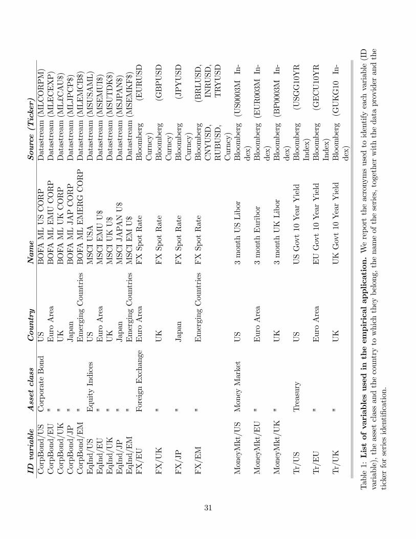
Details on the time series used in this paper are reported in Table 1. The data sources are
Datastream and Bloomberg. We embrace the MSCI definition of Emerging Markets and we
select the 5 most relevant countries in term of size of their economy, according to the ranking
based on the real annual GDP provided by the World Bank. Thus we select Brazil, India,
China, Russia and Turkey as Emerging Countries. We exclude from the analysis money
and treasury markets for Japan and Emerging Market, as the series were affected by excess
noise caused by measurement errors. We consider the US dollar as the numeraire: all the
series are US dollar denominated and the US dollar is the base rate for the FX pairs in the
dataset. In what follows, we consider simple weekly percentage returns for Equity Indices,
Bond Indices and Foreign Exchange Rates, whereas weekly first differences are considered for
Money Market and Goverment Rates series. In Table 2, we report some descriptive statistics
of the variables.
[Tables 1-2 about here]
The most remarkable facts are the extreme values which were recorded in correspondence
of the 2008-2009 crisis period. This is particularly evident for stock markets and for short
term rates, whereas along the country spectrum, the most hit were Emerging Markets. All
series exhibit the typical characteristic of non normality with high asymmetry and kurtosis.
6
The price series are plotted in Figure 1. The downturn at the end of the year 2008 is
immediately apparent and common to all the considered series.
[Figure 1 about here]
We propose a dynamic factor model with multiple sources of shocks, at global, asset class
and country level. In order to validate this approach, a first preliminary correlation analysis is
undertaken. Table 3 reports the in-sample correlation of the modelled variables. We observe
high correlation intra asset class groups. Particularly remarkable are the cases of equity and
treasury rates, with correlations in the 70-80% range. We observe substantial correlation even
within countries, in particular there is evidence of high interconnection between corporate
bonds and FX markets at country level: Euro Area (91.3%), Japan (83.6%) and UK (83.3%).
Hence, there is evidence for the presence of both an asset class and a country effect. However,
the asset class effect seems to be systematically more pervasive than the country one.
[Table 3 about here]
3 A Dynamic Multi-Factor Model
In this section, we present the modelling framework we propose. The main novelty of the
paper is the formulation and the estimation of a dynamic multi-factor model which allows to
test for the presence of contagion in the Forbes and Rigobon (2002) sense versus the presence
of volatility triggered episodes of excess interdependence on financial markets. Contagion
is no longer thought as correlation in excess of what implied by an economic model (as
in Bekaert et al. 2005 and Bekaert et al.2012), it instead corresponds to a specific market
situation, that the framework proposed in this paper is able to capture, entailing a persistent
change in financial linkages between markets
Building on the standard latent factor finance literature (Ross, 1976; Fama and French
1992), let Ri,jt represent the weekly return for the asset belonging to asset class i = 1, . . . , I
7

and county j = 1, . . . , J at time t. The general representation of the model is as follows:
Ri,jt = E[Ri,j
t ] + F i,jt βi,jt + εi,jt (1)
βi,jt = diag(1− φi,j)βi,j + diag(φi,j)βi,jt−1 + ψi,jZt−1 + ui,jt (2)
where E[Ri,jt ] is the expected return for asset class i in country j at time t, βi,jt is a vector of
dynamic factor loadings, mapping from the zero-mean factors F i,jt to the single asset returns.
We entertain the possibility that the factors F i,jt are heteroscedastic, that is E[F i,j
t
′F i,jt ] =
ΣF i,j ,t, where ΣF i,j ,t is the time-varying covariance matrix of the factors. εi,jt is assumed
to be white noise and independent of F i,jt . β
i,j is the long-run value of βi,jt , φi,j and ψi,j
are 3-dimensional vectors of parameters to be estimated, {ui,jt }t=1,...,T are independent and
normally distributed. We assume ui,jt to be independent of εi,jt . diag(·) is the diagonal
operator, transforming a vector into a diagonal matrix. Zt is a conditional variable controlling
for period of market distress.
Following Dungey and Martin (2007), different sources of shocks are considered, at global,
asset class and country level, in a latent factor framework. A first factor, denoted as Gt, is
designed to capture the shocks which are common to all financial assets modelled, whereas
Ait is the asset class specific factor for asset class i = 1, . . . , I and the country factor Cjt is
the country specific factor for county j = 1, . . . , J at time t. We denote F i,jt ≡ [Gt A
it C
jt ]
and, correspondingly, for the factor loading we specify βi,jt ≡ [γi,jt δi,jt λi,jt ]′.
The full model is a multi-factor model with dynamic factor loadings and heteroscedastic
factors. This model setting allows us to explore and characterize dynamically the comove-
ments among the considered assets. On the one hand, time-dependent exposures to different
shocks let us disentangle dynamically the different sources of comovement between financial
markets, namely distinguishing among shocks spreading at a global level, at the asset class
or rather at the country level. On the other hand, the presence of time-varying exposures
to common factors enables us to test for the presence of contagion, controlling at the same
time for excess interdependence induced by heteroscedasticity in the factors. In the follow-
8

ing sections, we explore the features of the model and use it to characterize financial market
comovements during crisis.
In Section 3.1, we describe the estimation of the factors F i,jt , whereas the estimation of
Zt−1 is presented in Section 3.2.
3.1 Factor Estimation
The factors F i,jt are estimated by means of principal component analysis (PCA). The choice of
PCA is dictated by model simplicity and interpretability, yet providing consistent estimates
of the latent factors1. The global factor G is extracted using the entire set of variables
considered, whereas the other two factors, asset class (A) and the country specific (C) are
extracted from the different asset class and country groups, respectively. In this setting, the
number of variables from which the factors are extracted, say K, is fixed and small, whilst
the number of observations T is large.
3.1.1 Global factor (G).
Let us first consider the global factor G. In order to estimate it, we define the series of the
demeaned returns as ri,jt ≡ Ri,jt − E[Ri,j
t ] and we stack them into the matrix r. We then
consistently estimate the variance-covariance matrix of r, say Σr, via maximum likelihood,
as
Σr ≡1
(T − 1)r′r (3)
Let (lk,wk) be the eigencouples referred to the covariance matrix Σr, with k = 1, . . . , K,
such that l1 ≥ l2 ≥ . . . ≥ lK . We estimate (lk,wk) by extracting the eigenvalue-eigenvector
couples from the estimated covariance matrix of the returns Σr, denoted as (lk, wk).
The estimate G of the common factor G is given by the principal component extracted
1In the factor model literature, consistency of the factor estimation is a well established result for thecase in which the factor loading is stable. In this paper, we make use of the limiting theory developed byStock and Watson (1998, 2002 and 2009) and Bates et al. (2013) for the case of instability of the factorloading, suggesting that factors are consistently estimated using principal components.
9

using the matrix Σr, that is:
G = rw1 (4)
G is a consistent estimator of the factor G. Indeed, from the standpoint that Σr is a
consistent estimator of Σr, we claim that, as a direct consequence of the invariance property
for maximum likelihood estimators, the estimated eigencouples (lk, wk) consistently estimate
(lk,wk). See Anderson (2003).
3.1.2 Asset class (A) and country specific (C) factors.
Following the same procedure used for the estimation of global factor, in order to estimate
the asset class and the country specific factors Ai and Cj (with i = 1, . . . , I and j =
1, . . . , J) respectively, we define ri ≡ [ri,jt ]j=1,...,J and rj ≡ [ri,jt ]i=1,...,I as the matrices of
returns referred to asset class i and country j, respectively. Denote as Σri and Σrj the
corresponding covariance matrix and let wi1 and w
j1 be the eigenvectors corresponding to
the largest eigenvalues of the estimates Σri and Σrj. The estimates of the asset class and the
country specific factors Ai and Cj are then given by:
Ai = riwi1 (5)
Cj = rjwj1 (6)
As we use demeaned returns, the extracted factors will have zero mean by construction.
For the sake of model interpretability, we orthogonalize the factors, so that the three
groups of factors are mutually independent. The preliminary correlation analysis presented
in Section 2 suggests that the asset class factors are more pervasive than the country ones.
So, we first orthogonalize the asset class factors with respect to the global factor. Then,
we orthogonalize the country factors with respect to the asset class and the global factors.
This ensures for instance that the US factor is independent of the global factor and of the
equity factor. The orthogonalization process, however, is not carried out within the groups
10
of factors, so then the equity factor might have a nonzero correlation with the bond factor,
and so the US factor with the EU factor. In the empirical section we report below, we show
that our results are robust to the case in which one orthogonalizes the country factors with
the global one and then the asset class factors with respect to the others.
3.2 Factor Loading Specification and Estimation
In our specification (2), Zt−1 is a control factor extracted from pure exogenous variables
and it is supposed to measure market nervousness and accounts for potential increase in
the factor loading during market distress periods. We get an estimate Zt−1 of Zt−1 via the
principal component extracted from the VIX, which is widely recognized as indicator of
market sentiment, the TED spread and the Libor-OIS spread for Europe, which measure the
perceived credit risk in the system. Widening spreads corresponds to a lack of confidence in
lending money on the interbank market over short-term maturities, together with a flight to
security in the form of overnight deposits at the lender of last resort.
Thus, the specification of (2) for the factor loadings βi,jt is now
βi,jt = diag(1− φi,j)βi,j + diag(φi,j)βi,jt−1 + ψi,jZt−1 + ui,jt (7)
The conditional time-varying factor loading specification2 (7) emphasizes that βi,jt tends
to its long-run value βi,j while following an autoregressive type of process of order one with
a purely exogenous variable Z. Being Z a zero-mean variable, βi,j can indeed be interpreted
as the long-run value for βi,jt .
Specification (7) nests two special cases. First, a static specification of the form:
βi,jt ≡ βi,j, ∀i = 1, . . . , I, ∀j = 1, . . . , J (8)
2Specification (7) is within the class of the so-called conditional time-varying factor loading approach (seeBekaert et al., 2009), where the factor loadings are assumed to follow a structural dynamic equation (see forinstance Baele et al., 2010) of the form βi,jt ≡ β(Ft−1, Xt)where {Ft}t=1,...,T is the information flow and Xt
is a set of conditional variables
11
where we assume that the exposure of all modelled variables to the different groups of
factors are kept constant through time.
A second nested case is a time-varying factor loading specification
βi,jt = diag(1− φi,j)βi,j + diag(φi,j)βi,jt−1 + ui,jt (9)
where it is assumed that no exogenous variables enter in the data generating process of
the betas. In Bekaert et al. (2009), the dynamics of the betas is specified using subsamples of
fixed length via a rolling window estimation, so that the factor loadings are constant within
pools of observations with the factor loadings having the following specification: βi,jt ≡
βi,j,s s = 1, . . . , S where βi,j,s is the static factor loading estimate referred to subsample s,
while S is the number of subsamples considered. Authors partition the sample in semesters
and re-estimate the model every six months. However, the rolling windows estimation is
based on changing subsamples of the data and it may not reflect time-variation fairly well
especially in small samples as also pointed out, amongst others, by Benarjee, Lumsdaine and
Stock (1992). Thus, in our paper we estimate specification (9) using Kalman Filter maximum
likelihood estimation to avoid both issues on potential inconsistency of the estimates obtained
using sub-samples and any arbitrary choice about the inertia, the subsample lenght, as to
which factor loadings evolve through time.
To summarise, our proposed dynamic multi-factor model is:
Ri,jt = E[Ri,j
t ] + F i,jt βi,jt + εi,jt (10)
βi,jt = diag(1− φi,j)βi,j + diag(φi,j)βi,jt−1 + ψi,jZt−1 + ui,jt (11)
OLS gives consistent estimates of (10) when using specification (8), corresponding to the
static case, which we consider the baseline. When considering the alternative specifications
(7) and (9), we allow that the factor loadings show evidence of contagion either in a con-
ditioned way (ψi,j 6= 0) or in an unconditioned way (ψi,j = 0) , according to the specified
12

control variable. In these other two cases, consistent estimates are obtained by applying the
Kalman filter. The models are nested and thus, the standard likelihood ratio test can be
employed for model selection.
3.3 Heteroscedastic Factors
We set up our modelling framework so that we can distinguish between spikes in comovements
due to increasing exposures to common risk factors from the case in which spikes are triggered
by excess volatility in the common factors. For this reason, besides allowing for dynamic
factor exposures, we allow for heteroscedastic factors. We model heteroscedasticity using
Engle’s (2002) Dynamic Conditional Correlations (DCC) model of order (1,1), and employing
a GARCH(1,1) for the marginal conditional volatility processes with normal innovations.
The extent that the three groups of factors are mutually independent by construc-
tion greatly simplifies the estimation. For the case of the global factor Gt, a univariate
GARCH(1,1) with normal innovation is employed to estimate time-varying volatility. For
the asset class and the country factors, we apply the Engle’s DCC model separately on
At and Ct, defined by stacking the factors into matrices as follows: At ≡ [Ait]i=1,...,I and
Ct ≡ [Cjt ]j=1,...,J . We obtain consistent estimates of the time-varying covariance matrices of
the factors, estimating the DCC model via quasi-maximum likelihood estimation.
3.4 Financial Markets Comovements: Contagion versus Excess
Interdependence
From the dynamic factor model introduced above, we can derive the time-varying covariance
between pairs of financial assets.
To simplifying the notation, let us introduce the one-to-one mapping n ≡ n(i, j), with
which we identify asset n (n = 1, . . . , N), belonging to asset class i and country j. Given
the independence between the factors Ft and the error term εt, from (1) it follows that the
13
covariance between asset n1 and asset n2 at time t is given by:
covt(Rn1 , Rn2) = E[βn1
t′F n1t′F n2t βn2
t ] + E[εn1t ε
n2t ] (12)
The first term on the right hand side is what is generally referred to as model implied
covariance, whereas the second is called residual covariance. The empirical counterpart of
(12) is given by:
ˆcovt(Rn1 , Rn2) = β
n1′t Σn1,n2
F,t βn2
t + Σn1,n2ε,t (13)
which we rewrite for convenience, as:
ˆcovn1,n2,t = ˆcovFn1,n2,t+ ˆcovεn1,n2,t
(14)
Correspondingly, define the quantities ˆcorrFn1,n2,tand ˆcorrεn1,n2,t
dividing by the appropriate
variances. We provide the estimates of ˆcorrεn1,n2,tvia the DCC framework. We deliberately
do not adjust the residuals of the model by heteroscedasticty and/or serial correlation, which
are instead treated as genuine features of the data. We denote the model implied variance
of the n-th market by ˆvarn,t, which is defined as ˆvarn,t ≡ ˆcovn,n,t.
During period of financial distress, soaring empirical covariances are in general observed.
Eq. (13) shows that the covariance between Rn1 and Rn2 can rise through three different
channels: an increase in the factor loadings βt, an increase in the covariance of the factors
ΣF,t, and an increase residual covariance Σε,t. Bekaert et al. (2005) and the related literature
identify contagion as the comovement between financial markets in excess of what implied
by an economic model. In this view, contagion is associated with spiking residual covariance
between markets, which refers to the second term on the right-hand side of both Eq. (13)
and Eq. (14). In our modelling set-up, we take a different stand. Consistently with the
case brought by Forbes and Rigobon (2002, pp. 2230-1), contagion is thought as an episode
of financial distress characterized by increasing interlinkages between markets. This extent
finds its model equivalent in a surge in the factor loadings βt. On the contrary, spiking
14

volatility in the factor conditional covariances is associated with excess interdependence. We
formalize this notion in Definition 1 (contagion) and Definition 2 (excess interdependence)
below.
Following Bekaert et al. (2009), we consider the average measure of model implied
comovements:
ΓFt ≡1
N(N − 1)/2
N∑n1=1
N∑n2>n1
ˆcorrFn1,n2,t(15)
and similarly we define Γεt as the residual comovement measure.
In order to characterize financial market comovements, we may assume that the residual
covariance ˆcovεn1,n2,tis negligible and focus our attention on the model implied covariance
ˆcovFn1,n2,t. There are two sources through which the covariance between two markets can
surge: an increase in the factor loadings βt, and/or increase in the factor volatilities ΣF,t.
In other words, assuming that our model fully captures the correlations between assets
(E[εn1t ε
n2t ] = 0), the possible sources of a surge in the comovements are either soaring factor
volatilities or increasing exposures to the factors. We label the former effect as contagion,
whereas we call the latter excess interdependence.
We can get further insights into the covariance decomposition outlined in (12), by recalling
that the factors F i,jt = [Gt A
it C
jt ] are by construction mutually independent. Thus, from
(12), it follows that:
covt(Rn1 , Rn2) = E[γn1
t′Gt′Gtγ
n2t ] + E[δn1
t′Ai1t
′Ai2t δ
n2t ] + E[λn1
t′Cj1
t
′Cj2t λ
n2t ] + E[εn1
t εn2t ] (16)
with empirical counterpart of the form:
covt(Rn1 , Rn2) = γn1′
t Σn1,n2
G,t γn2t + δ
n1′t Σn1,n2
A,t δn2
t + λn1′t Σn1,n2
C,t λn2
t + Σn1,n2ε,t (17)
which for convenience we write as:
ˆcovn1,n2,t = ˆcovGn1,n2,t+ ˆcovAn1,n2,t
+ ˆcovCn1,n2,t+ ˆcovεn1,n2,t
(18)
15
Our model framework has the advantage that it allows to discriminate among comovements
due to global, asset class or country specific shocks. We define a measure of comovement
prompted by the global factor as:
ΓGt ≡1
N(N − 1)/2
N∑n1=1
N∑n2>n1
ˆcorrGn1,n2,t(19)
where:
ˆcorrGn1,n2,t≡
ˆcovGn1,n2,t√ˆvarFn1,t
ˆvarFn2,t
(20)
and can be seen as the part of the correlation between markets n1 and n2, due to the common
dependence on the global factor. In the same manner, we define ΓAt and ΓCt as the measures
of comovements prompted by asset class and country factors, respectively. By construction
we have: ΓFt ≡ ΓGt + ΓAt + ΓCt .
We decline the same Γ-measures of comovements also at the asset class and country level.
Let Ii be the set of indices from the sequence n = 1, . . . , N referred to markets belonging to
the asset class i, and Jj be the indices referred to markets in country j, that is:
Ii ={n∣∣n = n(i, j); j = 1, . . . , J
}(21)
Jj ={n∣∣n = n(i, j); i = 1, . . . , I
}(22)
The model implied comovement measure for asset class i is given by:
Γit ≡1
|Ii| (|Ii| − 1) /2
∑n1∈Ii
∑n2∈Iin2>n1
ˆcorrFn1,n2,t(23)
and in the same manner for country j, we have:
Γjt ≡1
|Jj| (|Jj| − 1) /2
∑n1∈Jj
∑n2∈Jjn2>n1
ˆcorrFn1,n2,t(24)
16
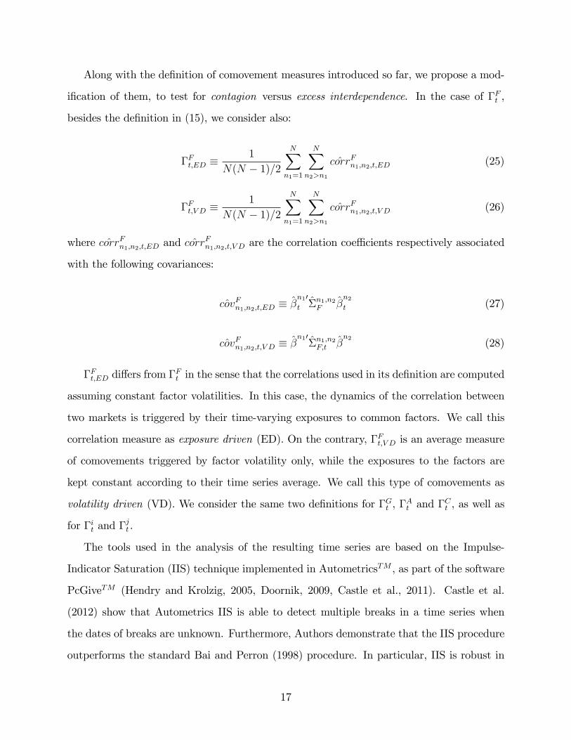
Along with the definition of comovement measures introduced so far, we propose a mod-
ification of them, to test for contagion versus excess interdependence. In the case of ΓFt ,
besides the definition in (15), we consider also:
ΓFt,ED ≡1
N(N − 1)/2
N∑n1=1
N∑n2>n1
ˆcorrFn1,n2,t,ED(25)
ΓFt,V D ≡1
N(N − 1)/2
N∑n1=1
N∑n2>n1
ˆcorrFn1,n2,t,V D(26)
where ˆcorrFn1,n2,t,EDand ˆcorrFn1,n2,t,V D
are the correlation coeffi cients respectively associated
with the following covariances:
ˆcovFn1,n2,t,ED≡ β
n1′t Σn1,n2
F βn2
t (27)
ˆcovFn1,n2,t,V D≡ β
n1′Σn1,n2
F,t βn2
(28)
ΓFt,ED differs from ΓFt in the sense that the correlations used in its definition are computed
assuming constant factor volatilities. In this case, the dynamics of the correlation between
two markets is triggered by their time-varying exposures to common factors. We call this
correlation measure as exposure driven (ED). On the contrary, ΓFt,V D is an average measure
of comovements triggered by factor volatility only, while the exposures to the factors are
kept constant according to their time series average. We call this type of comovements as
volatility driven (VD). We consider the same two definitions for ΓGt , ΓAt and ΓCt , as well as
for Γit and Γjt .
The tools used in the analysis of the resulting time series are based on the Impulse-
Indicator Saturation (IIS) technique implemented in AutometricsTM , as part of the software
PcGiveTM (Hendry and Krolzig, 2005, Doornik, 2009, Castle et al., 2011). Castle et al.
(2012) show that Autometrics IIS is able to detect multiple breaks in a time series when
the dates of breaks are unknown. Furthermore, Authors demonstrate that the IIS procedure
outperforms the standard Bai and Perron (1998) procedure. In particular, IIS is robust in
17

presence of outliers close to the end and the start of the sample3.
Following Castle et al. (2012), we look for structural breaks in the generic Γ(·)t average
comovement measures, by estimating the regression:
Γ(·)t = µ+ ηt (29)
where µ is a constant and ηt is assumed to be white noise. We then saturate the above
regression using the IIS procedure, which retains into the model individual impulse-indicators
in the form of spike dummy variables, signalling the presence of instabilities in the modelled
series. These dummies occur in block between the dates of the breaks. In line with the
procedure outlined in Castle et al. (2012), we group the dummy variables “with the same
sign and similar magnitudes that occur sequentially”to form segments of dummies, whereas
the impulse-indicators which can not be grouped will be labelled as outliers. We interpret
the segments of spike dummies as a step dummy for a particular regime. We can now state
the following:
Definition 1 (Contagion). A situation of contagion is identified when a segment of
dummy variables is detected through the IIS procedure for the average comovement measure
Γ(·)t,ED.
Definition 2 (Excess interdependence). A situation of excess interdependence is
identified when a segment of dummy variables is detected through the IIS procedure for the
average comovement measure Γ(·)t,V D.
We set a restrictive significance level of 1%, which leads to a parsimonious specification,
as shown in Castle et al. (2012). Section 4.2 gives account of the results of the outlined
methodology applied to our data.
3The use of the IIS strategy to identify structural breaks using a number of dummy variables has simi-larities to the contagion test proposed by Favero and Giavazzi (2002)
18

4 Empirical Results
In this section, we report the estimates of the dynamic multi-factor model formulated in
Section 3. In particular, in Section 4.1 we report the results of the estimation of the factors
and the specification of the factor loading, in Sections 4.2 the empirical analysis of market
comovements, both the estimates of measures of market comovements (Section 4.2.1) and the
regime of contagion vs excess interdependence we identify in market comovements (Section
4.2.2).
4.1 Factor Estimates and Factor Loading Selection
We start our empirical analysis by extracting the factors according to the methodology
outlined in Section 3.1. We extract the first principal component at a global, asset class and
country level from the estimate of the covariance matrix of the demeaned return time series.
The factors have by construction zero mean.
The extracted factors account in total for 83.28% of the overall variance, thus explaining
a substantial amount of the variation of the considered return series. In particular, the global
factor extracts as much as the 37.27% of the overall variance, whereas the asset class and
the country factors account for a quota in the 50− 80% range of the variation in the groups
they are extracted from.
We then orthogonalize the extracted factors, so that the system F i,jt ≡ [Gt A
it C
jt ] with
i = 1, . . . , I and j = 1, . . . , J consists of orthogonal factors. We first orthogonalize each of
the asset class factors with respect to the global factor and then orthogonalize the country
factors with respect to both the global and the asset class factors. In Section 4.2, we show
that all our main results do not depend on the particular way the orthogonalization is carried
out.
To validate the interpretations we attached to the factors, we map the contributions
of the original variables onto the factors via linear correlation analysis. The result of this
analysis is reported in Table 4.
19

[Table 4 about here]
We find that the stock indices are the most correlated with the global factors, with
correlations in the 80%-90% range. This characterizes the global factor as the momentum
factor. Such an interpretation seems reasonable in view of the fact that the equity asset class
can be thought as the most direct indicator of the financial activity among the asset classes
here considered.
More generally, when we sort the different markets by the magnitude of their correlation
with the global factor, they tend to group by asset class, rather then by country, with the
Treasury and the FX market figure in the 30%-50% range and the money market and the
corporate bond market in the 0%-30% range. This again supports the evidence that the
asset class effect is more pervasive than the country effect. The extent that the global factor
contains part of the asset class effect, however, does not pollute the interpretation of the
asset class factors, which remain positively and strongly correlated with the variables which
they are extracted from, even after the orthogonalization process.
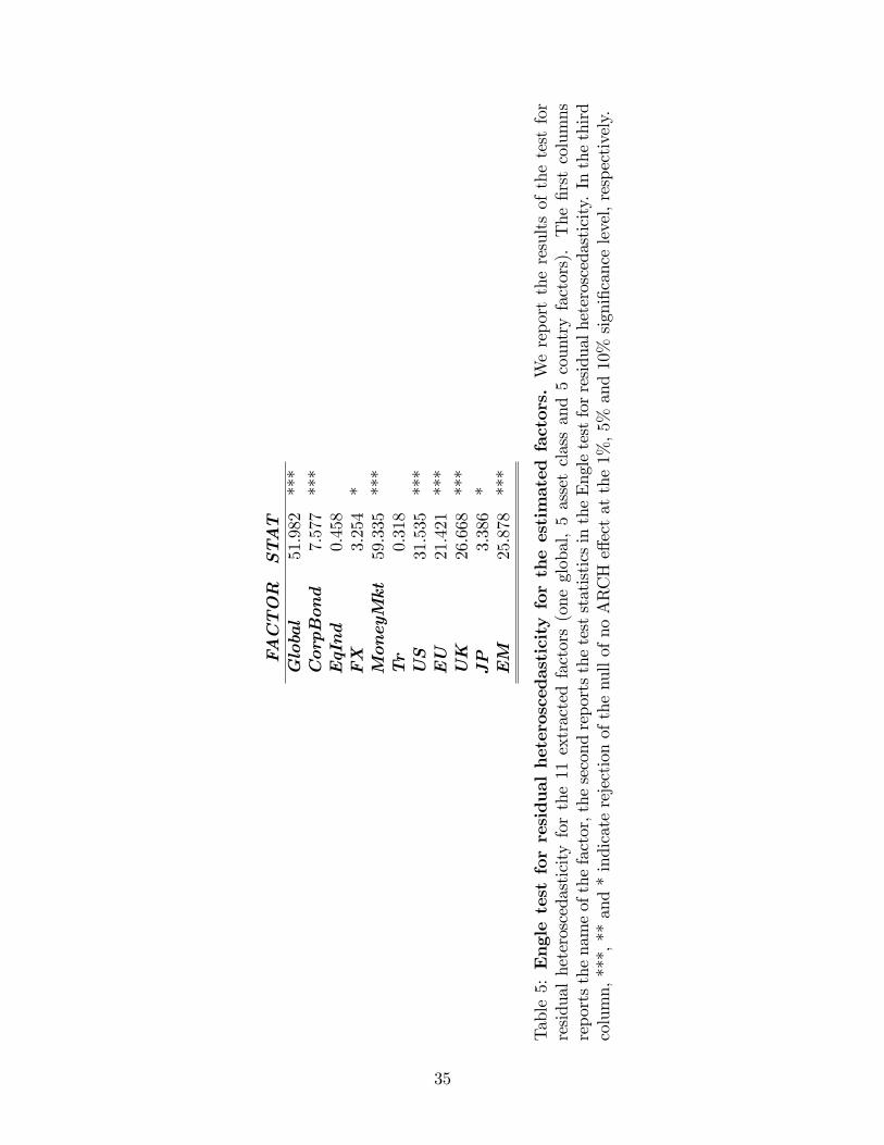
To test for excess interdependence prompted by changes in the volatility of the factors,
we entertain the possibility that the factor time series might be characterized by volatility
clustering. In Table 5, we report the Engle test for residual heteroscedasticity that suggests
that at the 1% confidence level this is indeed the case for 7 out of the 11 estimated factors.
[Table 5 about here]
We fit the Engle’s DCC model on the series of the estimated factors to get a time-varying
estimate of their covariance matrix.
We estimate (10) via OLS when we use the static formulation (8) for the factor loading,
while when the factor loadings are specified as in either the time-varying (9) or the conditional
time-varying factor loading (7) model, we estimate (10) via the Kalman filter using maximum
likelihood estimation method. The models are nested and thus the likelihood ratio test can
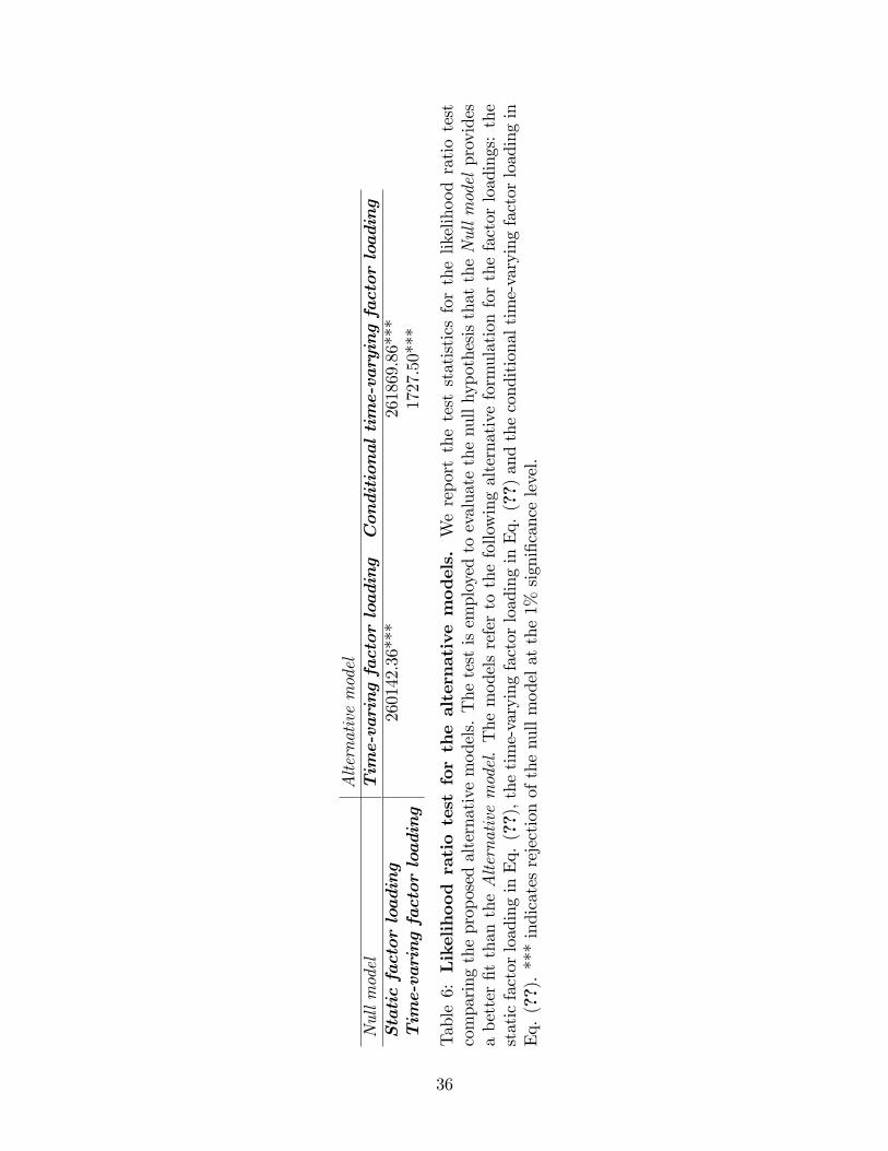
be employed for model selection. The likelihood ratio statistics are reported in Table 6.
[Table 6 about here]
20

The test strongly rejects the static alternative in favour of the dynamic ones. The con-
ditional time-varying factor loading approach dominates the time-varying factor loading
approach. Thus, there is evidence that the fitting of the model improves when we control
for market nervousness by means of the control factor Z.
4.2 Financial Market Comovements Dynamics
4.2.1 Measures of comovements
We turn now to analyse the average measures of comovements introduced in Section 3.4.
We start with the comparison between ΓFt and Γεt. The two measures are plotted in
Figure 2.
[Figure 2 about here]
As it can be clearly seen, the residual component is negligible throughout the sample pe-
riod and on average does not convey any information about the dynamics of the comovements
of the considered markets. We observed only a small jump in the idiosyncratic component in
correspondence to the late 2008, which has been considered by many the harshest period of
the 2007-09 global financial crisis. The model-implied measure of average comovements ΓFt
fluctuates around what can be regarded as a constant long-run value of roughly 20%. This
erratic behaviour does not allow us to identify any peak in correlation possibly associated
to crisis periods. During the period 2007-09 a slightly lower average correlations seem to be
observed instead. We give account of this fact in what follows, by disaggregating the model
implied covariation measure ΓFt .
We start doing this by considering the decomposition of the overall comovement measure
ΓFt into ΓGt , ΓAt and ΓCt , which is presented in Figure 3. The global factor appears to be
the most pervasive of all the three factors considered, shaping the dynamics of the average
overall measure. The asset class factor is slightly less pervasive, but it is the most persistent
of the three, meaning that its contribution is more resilient to change over time. This
expresses the fact that the characteristics which are common to the asset class contribute in
21
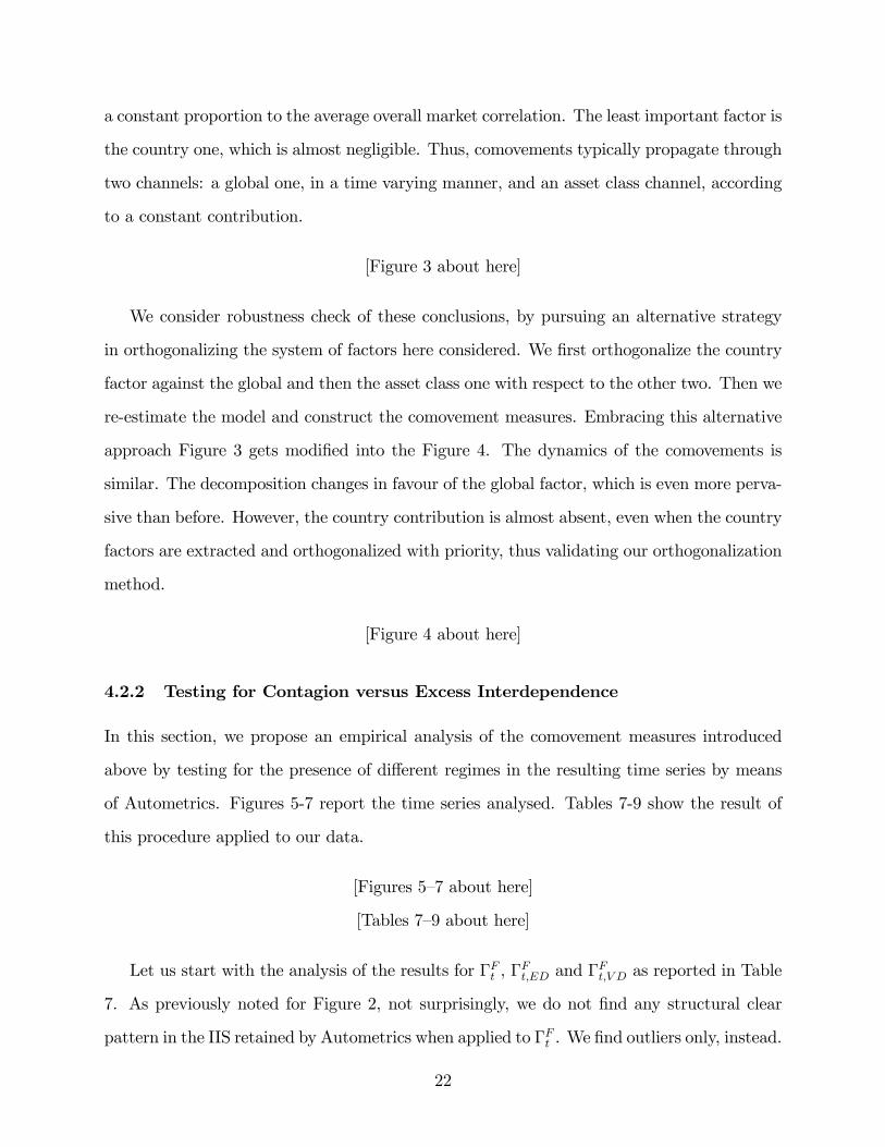
a constant proportion to the average overall market correlation. The least important factor is
the country one, which is almost negligible. Thus, comovements typically propagate through
two channels: a global one, in a time varying manner, and an asset class channel, according
to a constant contribution.
[Figure 3 about here]
We consider robustness check of these conclusions, by pursuing an alternative strategy
in orthogonalizing the system of factors here considered. We first orthogonalize the country
factor against the global and then the asset class one with respect to the other two. Then we
re-estimate the model and construct the comovement measures. Embracing this alternative
approach Figure 3 gets modified into the Figure 4. The dynamics of the comovements is
similar. The decomposition changes in favour of the global factor, which is even more perva-
sive than before. However, the country contribution is almost absent, even when the country
factors are extracted and orthogonalized with priority, thus validating our orthogonalization
method.
[Figure 4 about here]
4.2.2 Testing for Contagion versus Excess Interdependence
In this section, we propose an empirical analysis of the comovement measures introduced
above by testing for the presence of different regimes in the resulting time series by means
of Autometrics. Figures 5-7 report the time series analysed. Tables 7-9 show the result of
this procedure applied to our data.
[Figures 5—7 about here]
[Tables 7—9 about here]
Let us start with the analysis of the results for ΓFt , ΓFt,ED and ΓFt,V D as reported in Table
7. As previously noted for Figure 2, not surprisingly, we do not find any structural clear
pattern in the IIS retained by Autometrics when applied to ΓFt . We find outliers only, instead.
22

However, when looking at ΓFt,V D we find evidence of excess interdependence, that is excess
average correlation prompted by the heteroscedasticity of common factors, in correspondence
of the most severe period of the 2007-09 crisis, i.e. the last part of 2008, as well as in August
2011, when the sovereign debt crisis spread from the peripheral countries in Europe to the
rest of the continent and ultimately to the US. On the other hand, we detect a significant
negative break in the contagion measure ΓFt,ED from late 2007 to the end of 2008, which
offsets the peak in ΓFt,V D, so that no peaks are detected in ΓFt , as shown before. When
only factor exposures are concerned, we observe an average de-correlation of more than 6%.
We further disaggregate the Γ-measures at the asset class and country level. Along with
the detected segments, we observe a few outliers. In the case of ΓFt,ED, we find a couple of
outliers in proximity of the Dot-Com bubble burst, witnessing de-correlation on the market.
All the other IIS identified by Autometrics are in proximity of the start and the end of the
sample, a fact observed also in Castle et al. (2012).
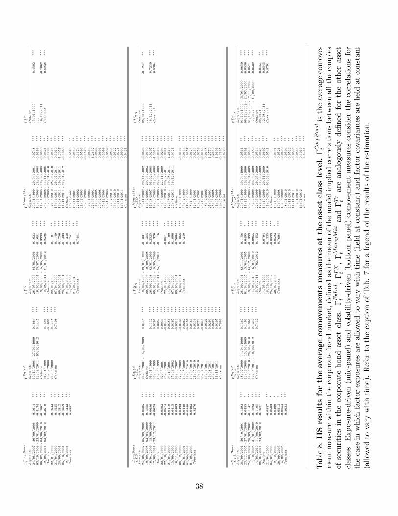
We turn our attention to Table 8 which reports the results referred to the single asset
classes. For stock indices, we find evidence of contagion from Aug-07 to mid-09, with corre-
lation significantly up by 5% from the average level of 79%. We also find evidence of excess
interdependence for three less extended periods, in correspondence of the most dramatic
months of 2008 and 2009, as well as in May-2010 and from Aug-2011 on, with a surge of
13-15% in the average correlation. We associate the former extent to the first EU interven-
tion in the Greece’s bailout programme, which marked the triggering of the sovereign debt
crisis in Europe. The second identified period has already been epitomized as the moment
in which the sovereign debt crisis spread across and outside Europe. At the aggregate level,
the 2007-09 crisis and the debt crisis remain the most relevant episodes in terms of average
market correlations.
Detecting contagion and excess interdependence in the stock markets during crisis is
very much in line with the mainstream literature on comovements. For the other asset
classes, the same periods are detected, but most of them are associated with decreasing
market correlations. This is particularly evident at the aggregate level for Corporate Bonds
23
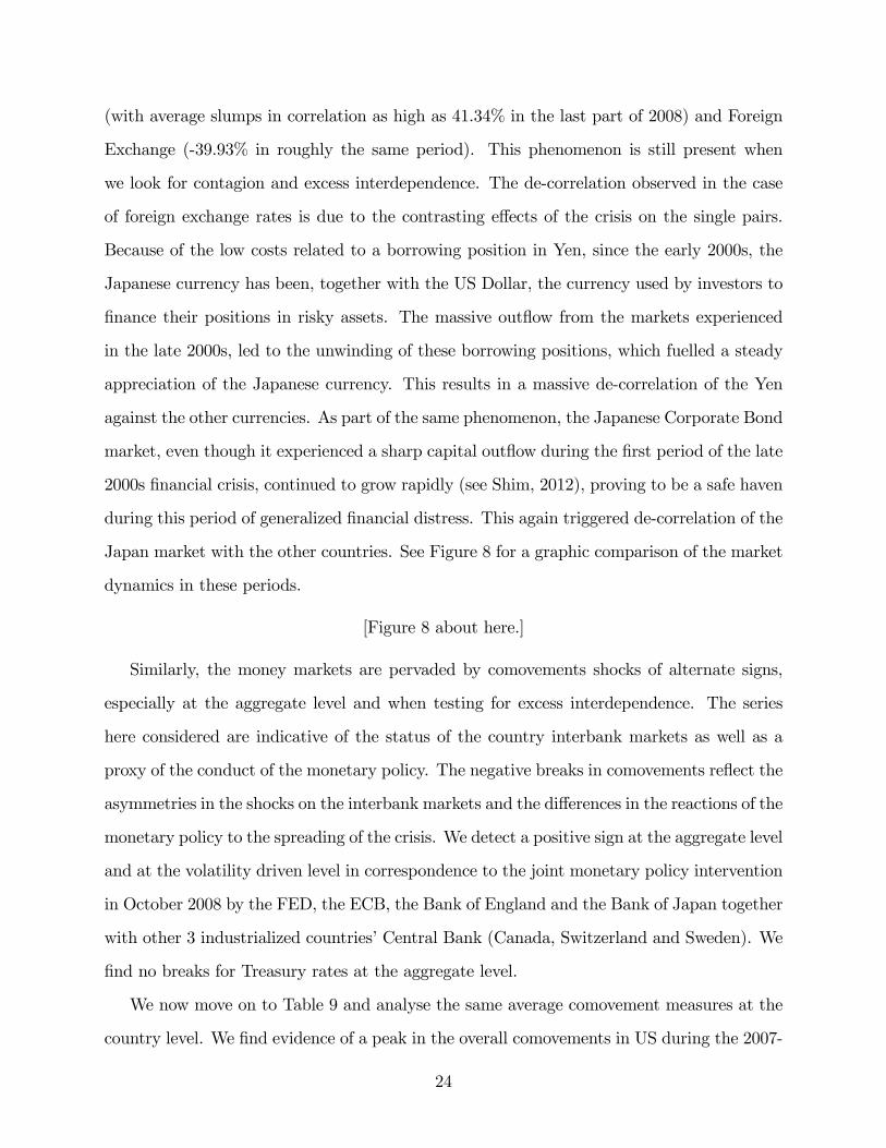
(with average slumps in correlation as high as 41.34% in the last part of 2008) and Foreign
Exchange (-39.93% in roughly the same period). This phenomenon is still present when
we look for contagion and excess interdependence. The de-correlation observed in the case
of foreign exchange rates is due to the contrasting effects of the crisis on the single pairs.
Because of the low costs related to a borrowing position in Yen, since the early 2000s, the
Japanese currency has been, together with the US Dollar, the currency used by investors to
finance their positions in risky assets. The massive outflow from the markets experienced
in the late 2000s, led to the unwinding of these borrowing positions, which fuelled a steady
appreciation of the Japanese currency. This results in a massive de-correlation of the Yen
against the other currencies. As part of the same phenomenon, the Japanese Corporate Bond
market, even though it experienced a sharp capital outflow during the first period of the late
2000s financial crisis, continued to grow rapidly (see Shim, 2012), proving to be a safe haven
during this period of generalized financial distress. This again triggered de-correlation of the
Japan market with the other countries. See Figure 8 for a graphic comparison of the market
dynamics in these periods.
[Figure 8 about here.]
Similarly, the money markets are pervaded by comovements shocks of alternate signs,
especially at the aggregate level and when testing for excess interdependence. The series
here considered are indicative of the status of the country interbank markets as well as a
proxy of the conduct of the monetary policy. The negative breaks in comovements reflect the
asymmetries in the shocks on the interbank markets and the differences in the reactions of the
monetary policy to the spreading of the crisis. We detect a positive sign at the aggregate level
and at the volatility driven level in correspondence to the joint monetary policy intervention
in October 2008 by the FED, the ECB, the Bank of England and the Bank of Japan together
with other 3 industrialized countries’Central Bank (Canada, Switzerland and Sweden). We
find no breaks for Treasury rates at the aggregate level.
We now move on to Table 9 and analyse the same average comovement measures at the
country level. We find evidence of a peak in the overall comovements in US during the 2007-
24
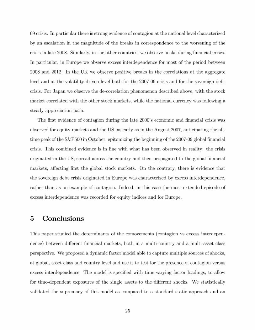
09 crisis. In particular there is strong evidence of contagion at the national level characterized
by an escalation in the magnitude of the breaks in correspondence to the worsening of the
crisis in late 2008. Similarly, in the other countries, we observe peaks during financial crises.
In particular, in Europe we observe excess interdependence for most of the period between
2008 and 2012. In the UK we observe positive breaks in the correlations at the aggregate
level and at the volatility driven level both for the 2007-09 crisis and for the sovereign debt
crisis. For Japan we observe the de-correlation phenomenon described above, with the stock
market correlated with the other stock markets, while the national currency was following a
steady appreciation path.
The first evidence of contagion during the late 2000’s economic and financial crisis was
observed for equity markets and the US, as early as in the August 2007, anticipating the all-
time peak of the S&P500 in October, epitomizing the beginning of the 2007-09 global financial
crisis. This combined evidence is in line with what has been observed in reality: the crisis
originated in the US, spread across the country and then propagated to the global financial
markets, affecting first the global stock markets. On the contrary, there is evidence that
the sovereign debt crisis originated in Europe was characterized by excess interdependence,
rather than as an example of contagion. Indeed, in this case the most extended episode of
excess interdependence was recorded for equity indices and for Europe.
5 Conclusions
This paper studied the determinants of the comovements (contagion vs excess interdepen-
dence) between different financial markets, both in a multi-country and a multi-asset class
perspective. We proposed a dynamic factor model able to capture multiple sources of shocks,
at global, asset class and country level and use it to test for the presence of contagion versus
excess interdependence. The model is specified with time-varying factor loadings, to allow
for time-dependent exposures of the single assets to the different shocks. We statistically
validated the supremacy of this model as compared to a standard static approach and an
25

alternative dynamic approach. The framework is applied to data covering 5 countries (US,
Euro, UK, Japan, Emerging), 5 asset markets (corporate bond yields, equity returns, cur-
rency returns relative to the US, short-term money market yields and long-term Treasury
yields) for a total of 20 series. The data are weekly beginning January 1999 and ending
March 2012.
The main findings of our empirical analysis can be summarized as follows. First, the
global factor is the most pervasive of the considered factors, shaping the dynamics of the
comovements of the considered financial markets. On the contrary, the asset class factor is
the most persistent through time, suggesting that the structural commonalities of markets
belonging to the same asset class systematically contributes in a constant proportion to the
average overall comovements. In our multiple asset class framework, the country factor is
negligible. In a robustness check, we showed that this result does not depend on the order
in which the system of factors is orthogonalized.
Secondly, we find evidence of contagion stemming from the US and the stock market
jointly in correspondence to the most harsh period of the 2007-09 financial crisis. On the
contrary, the currency and sovereign debt crisis originated in Europe characterized for the
presence of excess interdependence from mid-2010 onwards. According to the literature on
comovements, this let us characterize the spillover effects during the 2007-09 financial crisis
as persistent, altering the strength of the financial linkages worldwide. On the other hand,
the shock transmission experienced during the recent debt crisis has so far to be understood
as temporarily, being prompted by excess factor volatilities, which do not display trend in
the long-term.
Finally, at the overall average level, we do not find any evidence of contagion or excess
interdependence. We like to interpret this result as follows. During the crises some of the
securities considered in the study, the Japanese currency and corporate bond market in
particular, displayed a diverging dynamics as result of the unwinding of carry positions,
built to finance risky investments.
26
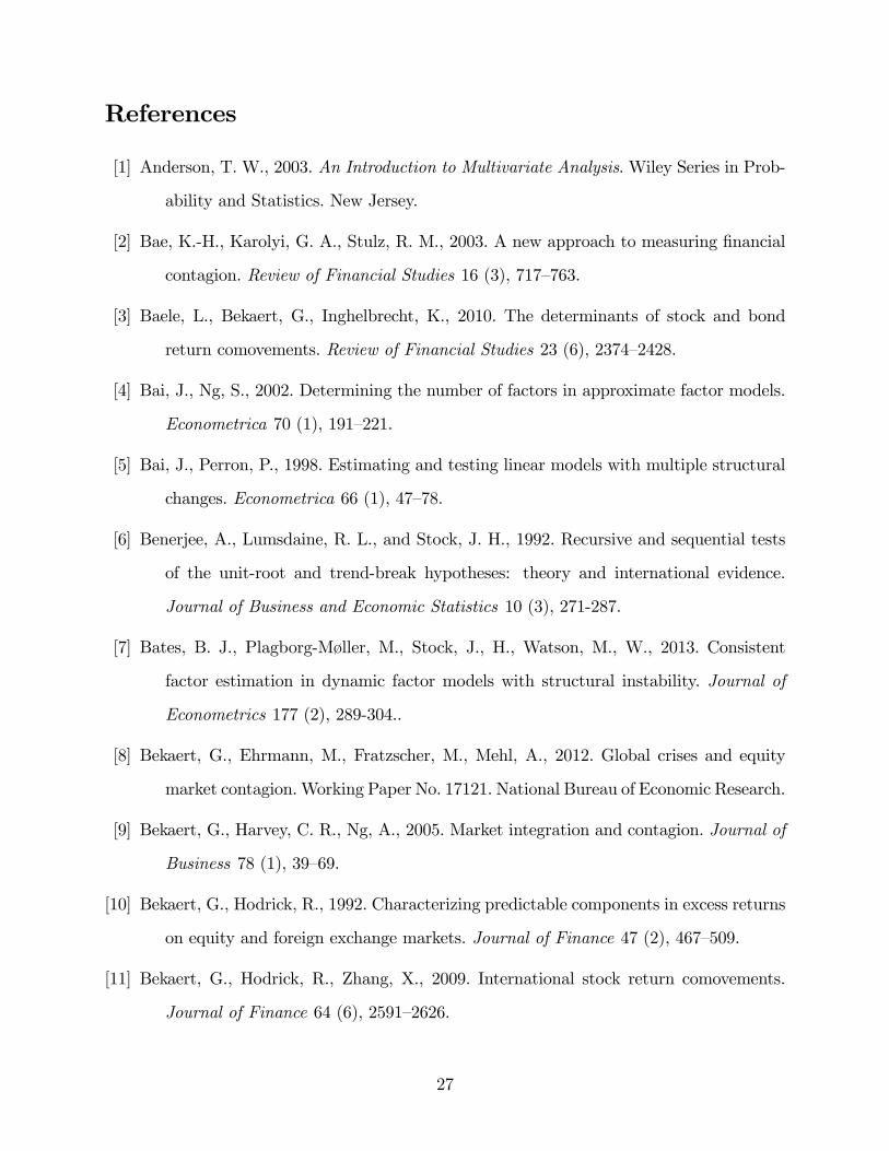
References
[1] Anderson, T. W., 2003. An Introduction to Multivariate Analysis. Wiley Series in Prob-
ability and Statistics. New Jersey.
[2] Bae, K.-H., Karolyi, G. A., Stulz, R. M., 2003. A new approach to measuring financial
contagion. Review of Financial Studies 16 (3), 717—763.
[3] Baele, L., Bekaert, G., Inghelbrecht, K., 2010. The determinants of stock and bond
return comovements. Review of Financial Studies 23 (6), 2374—2428.
[4] Bai, J., Ng, S., 2002. Determining the number of factors in approximate factor models.
Econometrica 70 (1), 191—221.
[5] Bai, J., Perron, P., 1998. Estimating and testing linear models with multiple structural
changes. Econometrica 66 (1), 47—78.
[6] Benerjee, A., Lumsdaine, R. L., and Stock, J. H., 1992. Recursive and sequential tests
of the unit-root and trend-break hypotheses: theory and international evidence.
Journal of Business and Economic Statistics 10 (3), 271-287.
[7] Bates, B. J., Plagborg-Møller, M., Stock, J., H., Watson, M., W., 2013. Consistent
factor estimation in dynamic factor models with structural instability. Journal of
Econometrics 177 (2), 289-304..
[8] Bekaert, G., Ehrmann, M., Fratzscher, M., Mehl, A., 2012. Global crises and equity
market contagion. Working Paper No. 17121. National Bureau of Economic Research.
[9] Bekaert, G., Harvey, C. R., Ng, A., 2005. Market integration and contagion. Journal of
Business 78 (1), 39—69.
[10] Bekaert, G., Hodrick, R., 1992. Characterizing predictable components in excess returns
on equity and foreign exchange markets. Journal of Finance 47 (2), 467—509.
[11] Bekaert, G., Hodrick, R., Zhang, X., 2009. International stock return comovements.
Journal of Finance 64 (6), 2591—2626.
27

[12] Billio, M., Caporin, M., 2010. Market linkages, variance spillovers, and correlation sta-
bility: Empirical evidence of financial contagion. Computational Statistics and Data
Analysis 54 (11), 2443—2458.
[13] Brandt, M. W., Brav, A., Graham, J. R., 2010. The idiosyncratic volatility puzzle: time
trend or speculative episodes? Review of Financial Studies 23 (2), 863—899.
[14] Castle, J.L., Doornik, J.A. and Hendry, D.F., 2011. Evaluating automatic model selec-
tion. Journal of Time Series Econometrics 3 (1), Article 8.
[15] Castle, J.L., Doornik, J.A. and Hendry, D.F., 2012. Model selection when there are
multiple breaks. Journal of Econometrics 169 (2), 239—246.
[16] Doornik, J.A., 2009. Autometrics. In: Castle and Shephard (2009), The Methodology
and Practice of Econometrics. Oxford University Press. Oxford.
[17] Driessen, J., Melenberg, B., Nijman, T., 2003. Common factors in international bond
returns. Journal of International Money and Finance 22 (5), 629—656.
[18] Dungey, M., Fry, R. E., González-Hermosillo, B., Martin, V. L., 2005. Empirical mod-
elling of contagion: a review of methodologies. Quantitative Finance 5 (1), 9—24
[19] Dungey, M., Martin, V., 2007. Unravelling financial market linkages during crises. Jour-
nal of Applied Econometrics 22 (1), 89—119.
[20] Ehrmann, M., Fratzscher, M., Rigobon, R., 2011. Stocks, bonds, money markets and
exchange rates: measuring international financial transmission. Journal of Applied
Econometrics 26 (6), 948—974.
[21] Engle, R. F., 2002. Dynamic conditional correlation. Journal of Business and Economic
Statistics 20 (3), 339—350.
[22] Engle, R. F., Ito, T., Lin, W., 1990. Meteor showers or heat waves? Heteroscedastic
intra-daily volatility in the foreign exchange market. Econometrica 58 (3), 525—542.
[23] Fama, E., French, K., 1993. Common risk factors in the returns on stocks and bonds.
Journal of Financial Economics 33 (1), 3—56.
28
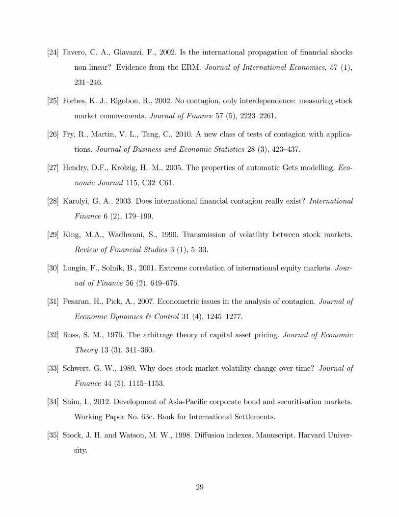
[24] Favero, C. A., Giavazzi, F., 2002. Is the international propagation of financial shocks
non-linear? Evidence from the ERM. Journal of International Economics, 57 (1),
231—246.
[25] Forbes, K. J., Rigobon, R., 2002. No contagion, only interdependence: measuring stock
market comovements. Journal of Finance 57 (5), 2223—2261.
[26] Fry, R., Martin, V. L., Tang, C., 2010. A new class of tests of contagion with applica-
tions. Journal of Business and Economic Statistics 28 (3), 423—437.
[27] Hendry, D.F., Krolzig, H.—M., 2005. The properties of automatic Gets modelling. Eco-
nomic Journal 115, C32—C61.
[28] Karolyi, G. A., 2003. Does international financial contagion really exist? International
Finance 6 (2), 179—199.
[29] King, M.A., Wadhwani, S., 1990. Transmission of volatility between stock markets.
Review of Financial Studies 3 (1), 5—33.
[30] Longin, F., Solnik, B., 2001. Extreme correlation of international equity markets. Jour-
nal of Finance 56 (2), 649—676.
[31] Pesaran, H., Pick, A., 2007. Econometric issues in the analysis of contagion. Journal of
Economic Dynamics & Control 31 (4), 1245—1277.
[32] Ross, S. M., 1976. The arbitrage theory of capital asset pricing. Journal of Economic
Theory 13 (3), 341—360.
[33] Schwert, G. W., 1989. Why does stock market volatility change over time? Journal of
Finance 44 (5), 1115—1153.
[34] Shim, I., 2012. Development of Asia-Pacific corporate bond and securitisation markets.
Working Paper No. 63c. Bank for International Settlements.
[35] Stock, J. H. and Watson, M. W., 1998. Diffusion indexes. Manuscript. Harvard Univer-
sity.
29

[36] Stock, J. H. and Watson, M. W., 2002. Forecasting using principal components from
a large number of predictors. Journal of the American Statistical Association 97,
1167– 1179.
[37] Stock, J. H. and Watson, M. W. (2009), Forecasting in dynamic factor models subject to
structural instability, in D. F. Hendry, J. Castle and N. Shephard, The Methodology
and Practice of Econometrics: A Festschrift in Honour of David F. Hendry, Oxford
University Press, pp. 173—205.
30
IDvariable
Assetclass
Country
Name
Source(Ticker)
CorpBond/US
CorporateBond
US
BOFA
MLUSCORP
Datastream(MLCORPM)
CorpBond/EU
"EuroArea
BOFA
MLEMUCORP
Datastream(MLECEXP)
CorpBond/UK
"UK
BOFA
MLUKCORP
Datastream(ML£CAU$)
CorpBond/JP
"Japan
BOFA
MLJAPCORP
Datastream(MLJPCP$)
CorpBond/EM
"EmergingCountries
BOFA
MLEMERGCORP
Datastream(MLEMCB$)
EqInd/US
EquityIndices
US
MSCIUSA
Datastream(MSUSAML)
EqInd/EU
"EuroArea
MSCIEMUU$
Datastream(MSEMUI$)
EqInd/UK
"UK
MSCIUKU$
Datastream(MSUTDK$)
EqInd/JP
"Japan
MSCIJAPANU$
Datastream(MSJPAN$)
EqInd/EM
"EmergingCountries
MSCIEMU$
Datastream(MSEMKF$)
FX/EU
ForeignExchangeEuroArea
FXSpotRate
Bloomberg
(EURUSD
Curncy)
FX/UK
"UK
FXSpotRate
Bloomberg
(GBPUSD
Curncy)
FX/JP
"Japan
FXSpotRate
Bloomberg
(JPYUSD
Curncy)
FX/EM
"EmergingCountries
FXSpotRate
Bloomberg
(BRLUSD,
CNYUSD,
INRUSD,
RUBUSD,
TRYUSD
Curncy)
MoneyMkt/US
MoneyMarket
US
3monthUSLibor
Bloomberg
(US0003M
In-
dex)
MoneyMkt/EU
"EuroArea
3monthEuribor
Bloomberg(EUR003M
In-
dex)
MoneyMkt/UK
"UK
3monthUKLibor
Bloomberg
(BP0003M
In-
dex)
Tr/US
Treasury
US
USGovt10YearYield
Bloomberg
(USGG10YR
Index)
Tr/EU
"EuroArea
EUGovt10YearYield
Bloomberg
(GECU10YR
Index)
Tr/UK
"UK
UKGovt10YearYield
Bloomberg
(GUKG10
In-
dex)
Table1:Listofvariablesusedintheempiricalapplication.Wereporttheacronymsusedtoidentifyeachvariable(ID
variable),theassetclassandthecountrytowhichtheybelong,thenameoftheseries,togetherwiththedataproviderandthe
tickerforseriesidentification.
31

Mean
StandardDeviation
Min
Max
Skewness
Kurtosis
CorpBond/US
0.119%
0.748%
-5.355%
3.171%
-0.935
8.553
CorpBond/EU
0.103%
1.558%
-5.815%
5.385%
-0.194
3.512
CorpBond/UK
0.100%
1.612%
-13.152%
5.628%
-1.075
10.651
CorpBond/JP
0.092%
1.347%
-5.356%
8.924%
0.572
6.755
CorpBond/EM
0.163%
0.826%
-9.332%
3.724%
-3.717
38.973
EqInd/US
0.014%
2.747%
-20.116%
11.526%
-0.748
8.850
EqInd/EU
-0.011%
3.502%
-26.679%
12.245%
-1.073
9.576
EqInd/UK
-0.009%
3.091%
-27.618%
16.243%
-1.249
14.920
EqInd/JP
0.009%
2.887%
-16.402%
11.016%
-0.258
4.823
EqInd/EM
0.184%
3.380%
-22.564%
18.538%
-0.775
8.889
FX/EU
0.017%
1.468%
-6.048%
4.992%
-0.213
3.831
FX/UK
-0.009%
1.341%
-8.348%
5.195%
-0.588
6.546
FX/JP
0.050%
1.498%
-6.027%
7.445%
0.253
4.304
FX/EM
-0.142%
1.517%
-17.401%
4.786%
-2.961
29.634
MoneyMkt/US
-0.350%
3.814%
-27.877%
21.137%
-1.850
16.873
MoneyMkt/EU
-0.187%
2.087%
-11.989%
15.021%
-0.717
11.723
MoneyMkt/UK
-0.262%
2.091%
-26.170%
8.374%
-4.357
43.968
Tr/US
-0.126%
3.596%
-19.122%
12.110%
-0.045
5.511
Tr/EU
-0.116%
3.056%
-17.838%
14.018%
-0.353
6.476
Tr/UK
-0.105%
2.805%
-16.758%
11.153%
-0.362
5.943
Table2:Descriptivestatisticsforthemarketreturns.Wereportsummarystatisticsforthevariableusedintheempirical
application.Thenumberreportedrefertotheentiresample,whichconsistsofweeklyobservationsfrom
Jan-1999toMar-2012.
32

CorpBond/US
CorpBond/EU
CorpBond/UK
CorpBond/JP
CorpBond/EM
EqInd/US
EqInd/EU
EqInd/UK
EqInd/JP
EqInd/EM
FX/EU
FX/UK
FX/JP
FX/EM
MoneyMkt/US
MoneyMkt/EU
MoneyMkt/UK
Tr/US
Tr/EU
CorpBond/EU
0.393
CorpBond/UK
0.462
0.694
CorpBond/JP
0.264
0.312
0.171
CorpBond/EM
0.578
0.539
0.516
0.046
EqInd/US
-0.041
0.087
0.080
-0.260
0.207
EqInd/EU
0.004
0.411
0.288
-0.161
0.351
0.785
EqInd/UK
0.028
0.326
0.403
-0.229
0.329
0.764
0.884
EqInd/JP
0.145
0.238
0.208
0.129
0.272
0.405
0.480
0.444
EqInd/EM
0.044
0.286
0.272
-0.211
0.448
0.693
0.785
0.755
0.545
FX/EU
0.178
0.913
0.566
0.232
0.402
0.126
0.435
0.333
0.217
0.291
FX/UK
0.162
0.616
0.833
0.060
0.358
0.156
0.373
0.502
0.251
0.336
0.642
FX/JP
0.181
0.295
0.138
0.836
0.054
-0.226
-0.112
-0.177
0.269
-0.140
0.262
0.101
FX/EM
0.079
0.349
0.296
-0.151
0.356
0.434
0.548
0.522
0.244
0.593
0.338
0.328
-0.094
MoneyMkt/US
-0.342
-0.233
-0.174
-0.133
-0.247
-0.020
-0.094
-0.091
-0.076
-0.088
-0.144
-0.081
-0.102
-0.077
MoneyMkt/EU
-0.177
-0.056
0.001
-0.009
-0.141
0.030
0.053
0.034
0.029
-0.005
0.015
0.036
-0.007
-0.018
0.385
MoneyMkt/UK
-0.227
-0.104
-0.002
-0.077
-0.245
0.061
-0.002
0.033
-0.017
-0.037
-0.023
0.119
-0.083
-0.003
0.536
0.525
Tr/US
-0.733
-0.246
-0.292
-0.388
-0.230
0.329
0.294
0.262
0.061
0.275
-0.104
-0.037
-0.295
0.152
0.141
0.112
0.090
Tr/EU
-0.548
-0.171
-0.280
-0.310
-0.152
0.297
0.337
0.276
0.114
0.277
0.045
0.040
-0.219
0.167
0.105
0.152
0.118
0.731
Tr/UK
-0.531
-0.205
-0.330
-0.313
-0.176
0.266
0.268
0.267
0.121
0.247
-0.031
0.083
-0.208
0.133
0.084
0.105
0.159
0.715
0.798
Table3:Samplecorrelationsamongthemarketreturns.
33

GlobalCorpBond
EqInd
FX
MoneyMkt
Tr
US
EU
UK
JPEM
CorpBond/US
-0.188
0.595
0.684
0.325
-0.337
-0.714
-0.234
0.017
0.032
0.098
0.059
CorpBond/EU
0.237
0.884
0.350
0.822
-0.211
-0.472
0.028
0.150
-0.120
-0.039
-0.044
CorpBond/UK
0.185
0.882
0.425
0.700
-0.131
-0.550
0.038
-0.163
0.145
0.052
-0.022
CorpBond/JP
-0.300
0.450
0.279
0.402
-0.128
-0.245
-0.106
0.107
-0.027
-0.129
0.015
CorpBond/EM
0.281
0.587
0.413
0.377
-0.248
-0.475
-0.007
-0.078
-0.153
0.061
0.278
EqInd/US
0.816
-0.072
0.248
-0.146
0.004
-0.214
0.138
-0.029
-0.035
-0.136
-0.167
EqInd/EU
0.907
0.193
0.275
0.127
-0.066
-0.284
-0.008
0.263
-0.024
-0.129
-0.156
EqInd/UK
0.875
0.206
0.290
0.119
-0.057
-0.307
-0.016
-0.011
0.312
-0.118
-0.188
EqInd/JP
0.541
0.177
0.350
0.096
-0.063
-0.288
-0.143
-0.181
-0.101
0.624
0.036
EqInd/EM
0.854
0.143
0.289
0.078
-0.072
-0.290
0.009
-0.177
-0.167
0.016
0.422
FX/EU
0.313
0.730
0.167
0.830
-0.117
-0.293
-0.012
0.226
-0.114
-0.078
-0.099
FX/UK
0.373
0.683
0.133
0.720
-0.032
-0.260
-0.061
-0.185
0.328
0.027
-0.092
FX/JP
-0.205
0.379
0.226
0.441
-0.104
-0.186
-0.089
0.044
-0.024
-0.026
0.022
FX/EM
0.557
0.225
0.122
0.421
-0.061
-0.222
0.119
-0.131
-0.169
0.088
0.212
MoneyMkt/US
-0.021
-0.241
-0.175
-0.139
0.973
0.187
0.133
-0.019
-0.034
-0.059
0.040
MoneyMkt/EU
0.092
-0.061
-0.138
-0.030
0.551
0.108
-0.360
0.152
-0.021
0.193
-0.096
MoneyMkt/UK
0.065
-0.104
-0.150
-0.010
0.697
0.118
-0.332
-0.031
0.176
0.120
-0.109
Tr/US
0.559
-0.474
-0.716
-0.350
0.153
0.738
0.309
-0.142
-0.123
-0.025
0.028
Tr/EU
0.577
-0.403
-0.700
-0.224
0.130
0.708
-0.229
0.248
-0.045
0.016
-0.025
Tr/UK
0.536
-0.439
-0.695
-0.239
0.118
0.712
-0.250
-0.059
0.266
0.023
-0.017
Table4:Correlationsbetweenthemarketreturnsandtheextractedfactors.Wereportthecorrelationbetweenthe
factorsandthemarketreturnsfrom
whichthefactorsareextracted.Thereare20seriesdisplayedintherowsand11factors
(oneglobal,5assetclassand5countryfactors),whicharedisplayedinthecolumns.Thenumbersreportedarein-samplelinear
correlations.
34
FACTOR
STAT
Global
51.982
***
CorpBond
7.577***
EqInd
0.458
FX
3.254*
MoneyMkt
59.335
***
Tr
0.318
US
31.535
***
EU
21.421
***
UK
26.668
***
JP3.386*
EM
25.878
***
Table5:Engletestforresidualheteroscedasticityfortheestimated
factors.Wereporttheresultsofthetestfor
residualheteroscedasticityforthe11extractedfactors(oneglobal,5assetclassand5countryfactors).Thefirstcolumns
reportsthenameofthefactor,thesecondreportstheteststatisticsintheEngletestforresidualheteroscedasticity.Inthethird
column,***,**and*indicaterejectionofthenullofnoARCHeffectatthe1%,5%
and10%significancelevel,respectively.
35
Alternativemodel
Nullmodel
Time-varingfactorloading
Conditionaltime-varyingfactorloading
Staticfactorloading
260142.36***
261869.86***
Time-varingfactorloading
1727.50***
Table6:Likelihoodratiotestforthealternativemodels.
Wereporttheteststatisticsforthelikelihoodratiotest
comparingtheproposedalternativemodels.ThetestisemployedtoevaluatethenullhypothesisthattheNullmodelprovides
abetterfitthantheAlternativemodel.Themodelsrefertothefollowingalternativeformulationforthefactorloadings:the
staticfactorloadinginEq.(??),thetime-varyingfactorloadinginEq.(??)andtheconditionaltime-varyingfactorloadingin
Eq.(??).***indicatesrejectionofthenullmodelatthe1%
significancelevel.
36

ΓFtOutliers26/02/1999 -0.0583 **. . .16/12/2011 -0.0584 **Constant 0.2230 ***
ΓFt,EDSegments17/08/2007 - 21/11/2008 -0.0670 ***Outliers07/04/2000 -0.0608 **30/06/2000 -0.0607 **09/03/2001 -0.0746 ***25/11/2011 -0.0646 ***02/12/2011 -0.0583 **Constant 0.2282 ***
ΓFt,V DSegments31/10/2008 - 05/12/2008 0.0564 ***12/08/2011 - 26/08/2011 0.0594 ***Outliers23/04/1999 -0.0507 ***Constant 0.2320 ***
Table 7: IIS results for the overall average comovement measures. ΓFt is the averagecomovement measure at the overall level, defined as the mean of the model implied corre-lations between all the couples of asset considered. ΓFt,ED (Γ
Ft,V D) considers the correlations
for the case in which factor exposures are allowed to vary with time (held at constant) andfactor covariances are held at constant (allowed to vary with time). We report the results ofthe saturation of model in Eq. (29) by means of Autometrics. We report the dates detectedvia the IIS technique, together with the estimated coeffi cients. Segment refers to group ofsequential dummies with the same size and similar magnitude. Outliers are dummies whichcan not be grouped. Constant refers to the constant term µ in Eq. 29 (***, ** and * indicatesignificance of the coeffi cient at the 1%, 5% and 10% significance level, respectively).
37
ΓCorpBond
tΓEqInd
tΓFX
tΓMoneyMkt
tΓTr
tSegments
Segments
Segments
Segments
Outliers
24/08/2007-26/09/2008
-0.1614
***
10/10/2008-27/03/2009
0.1664
***
26/05/2006-04/08/2006
-0.1623
***
29/01/1999-20/04/2001
-0.0748
***
15/01/1999
-0.4502
***
03/10/2008-23/01/2009
-0.4134
***
12/08/2011-03/02/2012
0.1447
***
16/03/2007-25/07/2008
-0.1681
***
14/03/2008-28/03/2008
-0.9199
***
...
06/02/2009-04/06/2010
-0.1867
***
Outliers
19/09/2008-15/05/2009
-0.3993
***
11/04/2008-19/09/2008
-0.0650
***
16/12/2011
-0.7062
***
12/08/2011-03/02/2012
-0.3610
***
01/01/1999
0.1596
***
12/08/2011-27/01/2012
-0.2528
***
26/09/2008-14/11/2008
0.0521
**
Constant
0.8238
***
Outliers
18/02/2000
-0.1695
***
Outliers
06/02/2009-22/01/2010
-0.1794
***
22/01/1999
-0.1643
***
24/03/2000
-0.1718
***
22/01/1999
-0.1107
**
07/05/2010-28/05/2010
0.0525
**
21/04/2000
-0.1535
***
Constant
0.7408
***
07/04/2000
-0.1149
***
15/04/2011-29/07/2011
-0.1010
***
28/09/2001
-0.1812
***
09/03/2001
-0.1756
***
12/08/2011-19/08/2011
-1.2057
***
05/10/2001
-0.1859
***
28/09/2001
-0.1433
***
11/11/2011-27/01/2012
-0.1060
***
12/10/2001
-0.1343
***
21/05/2004
-0.1340
***
Outliers
Constant
0.8557
***
24/07/2009
-0.1781
***
28/09/2001
0.0570
**
21/05/2010
-0.1111
**
16/11/2001
0.0550
**
Constant
0.7481
***
22/11/2002
-0.1174
***
21/02/2003
-0.0593
**
28/03/2003
-0.1570
***
04/04/2003
-0.0613
**
27/06/2003
-1.2632
***
01/02/2008
0.0524
**
29/02/2008
-0.0606
**
05/12/2008
-0.3098
***
26/12/2008
0.0502
**
02/07/2010
-0.0835
***
03/09/2010
0.0522
**
26/11/2010
-0.0771
***
14/01/2011
-0.0900
***
Constant
0.9421
***
ΓCorpBond
t,E
DΓEqInd
t,E
DΓFX
t,E
DΓMoneyMkt
t,E
DΓTr
t,E
D
Segments
Segments
Segments
Segments
Outliers
24/08/2007-05/09/2008
-0.0805
***
24/08/2007-15/05/2009
0.0448
***
19/03/1999-09/07/1999
-0.1037
***
08/11/2002-29/11/2002
-0.0623
***
08/01/1999
-0.1247
**
19/09/2008-03/04/2009
-0.1858
***
Outliers
20/05/2005-19/09/2008
-0.1385
***
14/02/2003-20/06/2003
-0.0190
***
...
10/04/2009-18/09/2009
-0.0686
***
01/01/1999
0.1132
***
26/09/2008-02/01/2009
-0.2525
***
17/08/2007-01/02/2008
-0.0207
***
16/12/2011
-0.7230
***
12/08/2011-23/12/2011
-0.0628
***
26/03/1999
0.0267
***
09/01/2009-15/05/2009
-0.1326
***
14/03/2008-21/03/2008
-1.3015
***
Constant
0.8304
***
Outliers
18/06/1999
0.0387
***
12/08/2011-25/11/2011
-0.1176
***
04/04/2008-24/04/2009
-0.0313
***
22/01/1999
-0.0803
***
02/03/2001
-0.0931
***
Outliers
05/06/2009-27/11/2009
-0.0204
***
22/10/1999
-0.0574
***
28/09/2001
-0.0413
***
22/01/1999
-0.0871
**
14/05/2010-29/07/2011
-0.0311
***
21/04/2000
-0.0419
***
05/10/2001
-0.0386
***
14/01/2000
-0.1109
***
12/08/2011-19/08/2011
-1.2619
***
15/09/2000
0.0415
***
15/03/2002
0.0367
***
07/04/2000
-0.1090
***
26/08/2011-16/12/2011
-0.0321
***
10/11/2000
0.0403
***
09/03/2007
-0.0312
***
09/03/2001
-0.2604
***
Outliers
08/12/2000
0.0493
***
17/07/2009
-0.0435
***
16/03/2001
0.1068
***
18/06/1999
-0.0142
***
05/01/2001
0.0440
***
14/08/2009
-0.0267
***
Constant
0.7349
***
30/07/1999
-0.0134
***
02/08/2002
-0.0440
***
12/03/2010
-0.0257
***
17/09/1999
0.0157
***
01/08/2003
0.0403
***
14/05/2010
-0.0460
***
08/10/1999
-0.0175
***
Constant
0.8276
***
21/05/2010
-0.0336
***
12/01/2001
-0.0233
***
20/08/2010
0.0271
***
10/08/2001
-0.0259
***
08/04/2011
-0.0345
***
28/12/2001
-0.0165
***
15/04/2011
-0.0522
***
08/02/2002
-0.0148
***
26/08/2011
0.0293
***
27/06/2003
-1.2770
***
23/09/2011
0.0290
***
28/03/2008
-0.2650
***
11/11/2011
0.0305
***
01/05/2009
-1.0106
***
Constant
0.7860
***
29/05/2009
-0.2165
***
Constant
0.9720
***
ΓCorpBond
t,V
DΓEqInd
t,V
DΓFX
t,V
DΓMoneyMkt
t,V
DΓTr
t,V
D
Segments
Segments
Segments
Segments
Segments
28/09/2001-26/10/2001
-0.1392
***
18/02/2000-14/04/2000
-0.1367
***
28/09/2001-02/11/2001
-0.1156
***
29/01/1999-30/04/1999
-0.0511
**
01/10/1999-05/05/2000
-0.0650
***
23/12/2005-27/01/2006
0.0485
*12/09/2008-13/03/2009
0.1491
***
01/04/2005-15/04/2005
0.0495
*17/12/1999-10/03/2000
-0.0891
***
06/12/2002-21/03/2003
-0.0536
***
24/08/2007-28/09/2007
-0.1147
***
14/05/2010-28/05/2010
0.1366
***
19/09/2008-04/12/2009
-0.1399
***
26/09/2008-16/01/2009
0.0540
**
31/10/2008-07/11/2008
0.0571
***
17/10/2008-31/07/2009
-0.1823
***
12/08/2011-10/02/2012
0.1347
***
14/05/2010-16/07/2010
-0.0955
***
06/02/2009-20/03/2009
-0.1680
***
17/04/2009-11/09/2009
-0.0502
***
14/05/2010-11/06/2010
-0.1108
***
Constant
0.7437
***
15/07/2011-17/02/2012
-0.1452
***
22/05/2009-29/05/2009
0.0534
**
Outliers
08/07/2011-24/02/2012
-0.1627
***
Outliers
17/07/2009-11/09/2009
0.0525
**
29/01/1999
-0.0454
**
Outliers
14/05/1999
-0.0794
***
16/10/2009-20/11/2009
-0.0697
***
12/08/2011
0.0545
***
21/04/2000
-0.0857
***
18/10/2002
-0.1335
***
07/05/2010-03/09/2010
0.0541
**
Constant
0.8791
***
04/07/2003
0.0503
*25/10/2002
-0.0899
***
Outliers
12/12/2003
0.0499
*30/07/2004
0.0523
*15/10/1999
0.0491
**
30/09/2005
0.0513
*Constant
0.7604
***
19/09/2008
-0.0521
**
15/02/2008
-0.0854
***
19/06/2009
-0.0690
***
Constant
0.8623
***
08/01/2010
-0.0504
**
26/11/2010
-0.0522
**
11/11/2011
-0.0583
**
06/01/2012
-0.0865
***
13/01/2012
-0.1019
***
Constant
0.9401
***
Table8:IISresultsfortheaveragecomovementsmeasuresattheassetclasslevel.
ΓCorpBond
tistheaveragecomove-
mentmeasurewithinthecorporatebondmarket,definedasthemeanofthemodelimpliedcorrelationsbetweenallthecouples
ofsecuritiesinthecorporatebond
assetclass.
ΓEqInd
t,
ΓFX
t,
ΓMoneyMkt
tand
ΓTr
tareanalogouslydefinedfortheotherasset
classes.Exposure-driven(mid-panel)andvolatility-driven(bottompanel)comovementmeasuresconsiderthecorrelationsfor
thecaseinwhichfactorexposuresareallowedtovarywithtime(heldatconstant)andfactorcovariancesareheldatconstant
(allowedtovarywithtime).RefertothecaptionofTab.7foralegendoftheresultsoftheestimation.
38
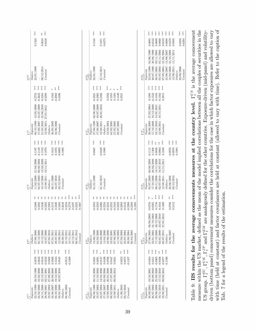
ΓUS
tΓEU
tΓUK
tΓJPt
ΓEM
t
Segments
Outliers
Segments
Segments
Ouliers
22/10/1999-29/10/1999
0.0576
***
27/06/2008
-0.2400**
11/02/2000-21/04/2000
0.1197
***
08/10/1999-12/05/2000
-0.2752***
22/01/1999
0.1323
***
04/02/2000-18/02/2000
0.0643
***
05/12/2008
0.2282
**04/07/2003-08/08/2003
-0.1149***
17/08/2007-24/07/2009
-0.3622***
...
24/11/2000-22/12/2000
0.0516
***
19/12/2008
0.2436
**10/10/2008-13/03/2009
0.1552
***
21/05/2010-25/06/2010
-0.2484***
09/12/2011
0.0618
**28/09/2001-02/11/2001
-0.0532***
10/07/2009
-0.2203**
12/08/2011-18/11/2011
0.1079
***
12/08/2011-27/01/2012
-0.3288***
Constant
0.6248
***
19/07/2002-27/09/2002
0.0568
***
07/05/2010
-0.2203**
Outliers
Outliers
24/08/2007-26/09/2008
0.0566
***
07/01/2011
-0.2155**
06/11/2009
0.1012
***
30/05/2003
0.1582
*03/10/2008-19/12/2008
0.1524
***
29/07/2011
0.2320
**16/07/2010
0.1076
***
16/06/2006
-0.2002**
02/01/2009-16/07/2010
0.0545
***
12/08/2011
0.2404
**03/12/2010
-0.0992***
Constant
0.3496
***
Outliers
26/08/2011
0.2648
**Constant
0.1988
***
08/08/2003
-0.0515***
21/10/2011
0.2253
**Constant
-0.1399***
18/11/2011
0.2779
***
23/12/2011
0.2197
**06/01/2012
0.2225
**Constant
0.1667
***
ΓUS
t,ED
ΓEU
t,ED
ΓUK
t,ED
ΓJPt,ED
ΓEM
t,ED
Segments
Ouliers
Outliers
Segments
Outliers
06/08/1999-08/12/2000
0.0331
***
13/08/1999
-0.2253**
01/01/1999
0.0567
***
27/08/1999-02/06/2000
-0.2321***
22/01/1999
0.1545
***
19/07/2002-11/10/2002
0.0291
***
04/02/2000
-0.2319**
...
17/08/2007-10/07/2009
-0.3365***
...
23/07/2004-14/04/2006
-0.0147*
03/03/2000
-0.2266**
01/10/2010
-0.0249***
12/08/2011-20/01/2012
-0.2486***
21/10/2011
0.1071
***
17/08/2007-05/09/2008
0.0436
***
14/04/2000
-0.2216**
Constant
0.1989
***
Outliers
Constant
0.6273
***
12/09/2008-30/01/2009
0.0766
***
23/06/2000
-0.2245**
12/03/2004
0.2703
***
06/02/2009-17/07/2009
0.0447
***
23/02/2001
-0.2252**
04/02/2005
0.1355
*12/08/2011-09/03/2012
0.0331
***
07/06/2002
-0.2163**
27/05/2005
0.1404
*Outliers
11/10/2002
-0.2222**
08/07/2005
0.1449
*11/06/2010
0.0252
**07/03/2003
-0.2263**
Constant
0.3521
***
03/12/2010
0.0275
***
23/07/2004
-0.2145**
Constant
-0.1457***
20/08/2004
-0.2269**
08/04/2005
-0.2288**
Constant
0.1805
***
ΓUS
t,VD
ΓEU
t,VD
ΓUK
t,VD
ΓJPt,VD
ΓEM
t,VD
Segments
Segments
Segments
Segments
Segments
28/09/2001-19/10/2001
-0.0484***
27/06/2003-08/08/2003
-0.0716**
04/07/2003-08/08/2003
-0.1111***
20/06/2003-27/02/2004
0.1288
***
23/04/1999-04/06/1999
0.0683
***
26/07/2002-20/09/2002
0.0451
***
23/01/2004-01/10/2004
-0.0565*
17/10/2008-20/03/2009
0.1308
***
17/10/2008-19/12/2008
-0.1532***
30/07/1999-20/08/1999
-0.0542***
20/06/2008-25/09/2009
-0.0365***
17/10/2008-26/12/2008
0.1748
***
06/11/2009-13/11/2009
0.0826
**19/11/2010-14/01/2011
0.1434
***
26/01/2001-02/11/2001
0.0680
***
19/11/2010-17/12/2010
-0.0336**
02/01/2009-23/07/2010
0.1044
***
02/07/2010-16/07/2010
0.0863
**12/08/2011-18/11/2011
-0.1162***
05/07/2002-01/11/2002
0.0660
***
19/08/2011-09/03/2012
-0.0377***
08/07/2011-27/01/2012
0.1300
***
12/08/2011-11/11/2011
0.1050
***
Constant
0.2815
***
07/05/2004-21/05/2004
0.0519
***
Constant
-0.1346***
Outliers
Outliers
24/08/2007-14/09/2007
0.0688
***
31/08/2007
0.0796
**20/06/2008
-0.0976***
18/04/2008-31/10/2008
0.0479
***
Constant
0.2112
***
03/12/2010
-0.0978***
12/08/2011-11/11/2011
0.0505
***
Constant
0.1994
***
Outliers
29/09/2000
0.0593
***
Constant
0.6394
***
Table9:IISresultsfortheaveragecomovementsmeasuresatthecountry
level.
ΓUS
tistheaveragecomovement
measurewithintheUSmarket,definedasthemeanofthemodelimpliedcorrelationsbetweenallthecouplesofsecuritiesinthe
USgroup.
ΓEU
t,Γ
UK
t,Γ
JPtand
ΓEM
tareanalogouslydefinedfortheothercountries.Exposure-driven(mid-panel)andvolatility-
driven(bottompanel)comovementmeasuresconsiderthecorrelationsforthecaseinwhichfactorexposuresareallowedtovary
withtime(heldatconstant)andfactorcovariancesareheldatconstant(allowedtovarywithtime).Refertothecaptionof
Tab.7foralegendoftheresultsoftheestimation.
39
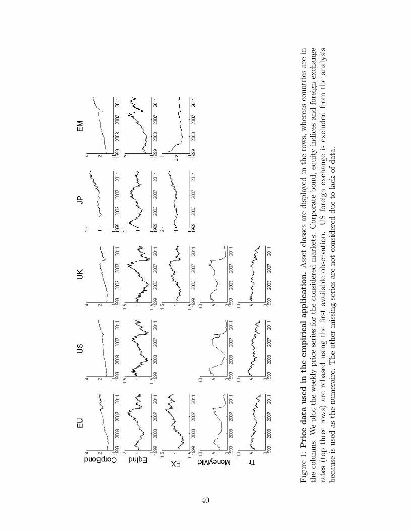
Figure1:Pricedatausedintheempiricalapplication.Assetclassesaredisplayedintherows,whereascountriesarein
thecolumns.Weplottheweeklypriceseriesfortheconsideredmarkets.Corporatebond,equityindicesandforeignexchange
rates(topthreerows)arerebasedusingthefirstavailableobservation.
USforeignexchangeisexcludedfrom
theanalysis
becauseisusedasthenumeraire.Theothermissingseriesarenotconsideredduetolackofdata.
40

Figure2:Modelimplied
versusresidualaveragecorrelationmeasures.
ΓF tistheaveragecomovementmeasureatthe
overalllevel,definedasthemeanofthemodelimpliedcorrelationsbetweenallthecouplesofassetconsidered.
Γε tistheaverage
residualcomovementmeasure,definedasthemeanofthecorrelationsbetweentheerrorterm
inthemodelforallthecouples
ofassetconsidered.
41
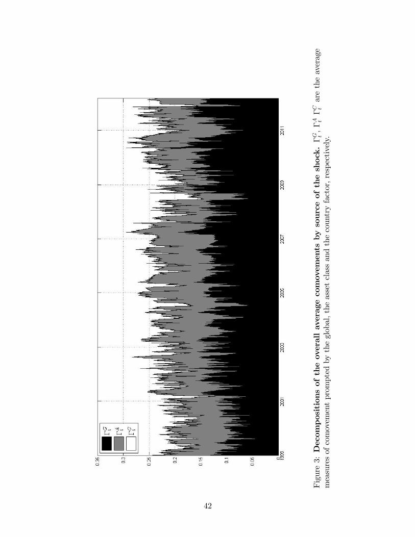
Figure3:Decompositionsoftheoverallaveragecomovementsby
sourceoftheshock.
ΓG t,
ΓA t
ΓC taretheaverage
measuresofcomovementpromptedbytheglobal,theassetclassandthecountryfactor,respectively.
42
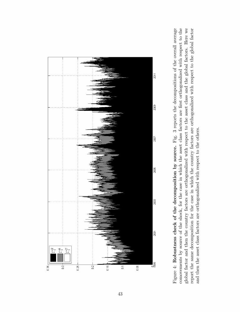
Figure4:Robustnesscheckofthedecompositionby
source.Fig.3reportsthedecompositionsoftheoverallaverage
comovementsbysourceoftheshock,forthecaseinwhichtheassetclassfactorsarefirstorthogonalizedwithrespecttothe
globalfactorandthenthecountryfactorsareorthogonalizedwithrespecttotheassetclassandtheglobalfactors.Herewe
reportthesamedecompositionforthecaseinwhichthecountryfactorsareorthogonalizedwithrespecttotheglobalfactor
andthentheassetclassfactorsareorthogonalizedwithrespecttotheothers.
43

Figure5:Averagecorrelationmeasures.
ΓF t(toppanel)istheaveragecomovementmeasureattheoveralllevel,defined
asthemeanofthemodelimpliedcorrelationsbetweenallthecouplesofassetconsidered.
ΓF t,ED-midpanel-(Γ
F t,VD-bottom
panel-)considersthecorrelationsforthecaseinwhichfactorexposuresareallowedtovarywithtime(heldatconstant)and
factorcovariancesareheldatconstant(allowedtovarywithtime).
44

Figure6:Averagecorrelationmeasuresattheassetclasslevel.
ΓCorpBond
tistheaveragecomovementmeasurewithin
thecorporatebondmarket,definedasthemeanofthemodelimpliedcorrelationsbetweenallthecouplesofsecuritiesinthe
corporatebondassetclass.
ΓEqInd
t,Γ
FX
t,Γ
MoneyMkt
tand
ΓTr
tareanalogouslydefinedfortheotherassetclasses.Exposure-driven
(secondcolumn)andvolatility-driven(thirdcolumn)comovementmeasuresconsiderthecorrelationsforthecaseinwhichfactor
exposuresareallowedtovarywithtime(heldatconstant)andfactorcovariancesareheldatconstant(allowedtovarywith
time).
45

Figure7:Average
correlationmeasuresatthecountrylevel.
ΓUS
tistheaveragecomovementmeasurewithintheUS
market,definedasthemeanofthemodelimpliedcorrelationsbetweenallthecouplesofsecuritiesintheUSgroup.
ΓEU
t,
ΓUK
t,
ΓJPtand
ΓEM
tareanalogouslydefinedfortheothercountries.Exposure-driven(secondcolumn)andvolatility-driven(third
column)comovementmeasuresconsiderthecorrelationsforthecaseinwhichfactorexposuresareallowedtovarywithtime
(heldatconstant)andfactorcovariancesareheldatconstant(allowedtovarywithtime).
46

Figure8:Comparison
amongselected
securitiesduringthedetectedregimes.Wereportcorporatebondandforeign
exchangepricelevelsforperiodsinwhichdecorrelationwasdetected.Thepricearerebasedusingthefirstobservationineach
subperiod.
47