Embed Size (px)
Citation preview

Professor Roger A. Falconer FREng Professor of Water Management and
Past President of IAHR (2011-15)
Hydro-environmental Research Centre
School of Engineering, Cardiff University
Modelling Extreme Flood Events
and Associated Processes

• Flooding essentially a natural process we need to live
with rivers, climate change and increasing storm events
Flooding not only be caused by high rainfall also poor
drainage, groundwater saturation, debris flows etc.
Flooding usually also leads to water pollution large loss
of life in many countries due to epidemiological outbreaks
Flooding damage extent often exacerbated by:
Inadequate data, poor warning systems and planning
Inadequate defences and insufficient upstream storage
Use of crude modelling tools and inexperienced operators
General

Floods are on the Rise

Floods Cause Loss of Life

Floods Bring Misery and Stress

Floods Bring Contamination

Cumbria Floods 2016 – Short Steep River Basin

Somerset Levels 2014 – Mild Slope River Basin

• Increasing concern of flooding along steep river basins and levee breeches – particularly in Wales
• Traditional 2-D and 1-D models not ideal for such flows and need refining for trans- and supercritical flows
• Full shallow water equations solved using a finite volume scheme on a collocated grid
• Model also refined to include surface and sub-surface flow interactions and extended to include floodplain flows in urban regions
Overview of Research for Steep Catchments

DIVAST-ADI vs. DIVAST-TVD
Dam-Break Problem
h 1
h 0

DIVAST-ADI vs. DIVAST-TVD
6
8
10
De
pth
(m)
0
50
100
150
200
x (m)
0
50
100
150
200
y (m)
h0 = 5 m
= 10-6 m2/s
6
8
10
De
pth
(m)
0
50
100150
200
x (m)
0
50
100
150
200
y (m)
h0 = 5 m
= 10-6 m2/s
DIVAST-ADI DIVAST-TVD

Dyke Break Experiment (TU Delft)
Gate

Dyke Break Experiment

Dyke Break Experiment
Time (s)
De
pth
(m)
0 5 10 15 200
0.05
0.1
0.15
Measured
Computed
Time (s)
De
pth
(m)
0 5 10 15 200
0.05
0.1
0.15
Measured
Computed
Time (s)
De
pth
(m)
0 5 10 15 200
0.05
0.1
0.15
Measured
Computed
Time (s)
De
pth
(m)
0 5 10 15 200
0.05
0.1
0.15
Measured
Computed

• Three modelling approaches considered:
Modelling buildings as solid blocks making buildings impervious
Remove buildings and increase local roughness not ideal
for water quality predictions
Remove buildings and treat as porous media better for
predicting water quality in buildings
Refined Treatment of Buildings

Flood Building Interaction
Unit: m
10
20
100 300
20
0
100
Dyke
Square Building
Reservoir
Manning’s n = 0.015

Flood Building Interaction 1 – Solid Building
Model Building
as solid block
Without Building

Flood Building Interaction 2 – High Roughness
n = 0.01 n = 0.03
n = 0.1 n = 5.0

Flood Building Interaction 3 – Porous Media
K = 250 m/s K = 50 m/s
K = 1 m/s K = 10 m/s

Flood Building Interaction – Water Levels
Time (s)E
levatio
n(m
)
0 60 120 1800
0.05
0.1
0.15
0.2
0.25
n=0.011
n=0.03
n=0.1
n=0.2
n=0.5
n=5.0
Solid
Time (s)
Ele
vatio
n(m
)
0 60 120 1800
0.2
0.4
0.6
0.8
Solid
n=5.0
n=0.5
n=0.2
n=0.1
n=0.03
n=0.011
Time (s)
Ele
vatio
n(m
)
0 60 120 1800
0.05
0.1
0.15
0.2
K=250
K=50
K=20
K=10
K=5
K=1
Solid
Time (s)
Ele
vatio
n(m
)
0 60 120 1800
0.2
0.4
0.6
0.8
Solid
K=1
K=5
K=10
K=20
K=50
K=250
Before Building After Building

Flood Inundation of Glasgow
Without buildings With buildings
City in Scotland prone to urban flooding

Flood Inundation of Glasgow
Porous media and solid block methods
Without buildings With buildings

Interaction Between Flood and Buildings
Water depth variance at G3:
t (min)
Ele
vatio
n(m
)
0 30 60 90 12023.6
23.8
24.0
24.2
24.4
Local high roughness method
K=0.1 m/s, Φ=0.8
K=0.1 m/s, Φ=0.5
Solid block method

• Small picturesque town in South West of UK
• Short river basin with steep valley terrain similar to
many river basins in Wales and Northern England
• Up to 200 mm rainfall fell in 5 hr and predicted to have 1 in 400 yr return period event
• Extensive damage to properties, bridges, highways and other infrastructure
• One of best recorded extreme flood events in UK with trans- and super-critical flows
Boscastle Flood 2004

View of Boscastle and Valency Valley


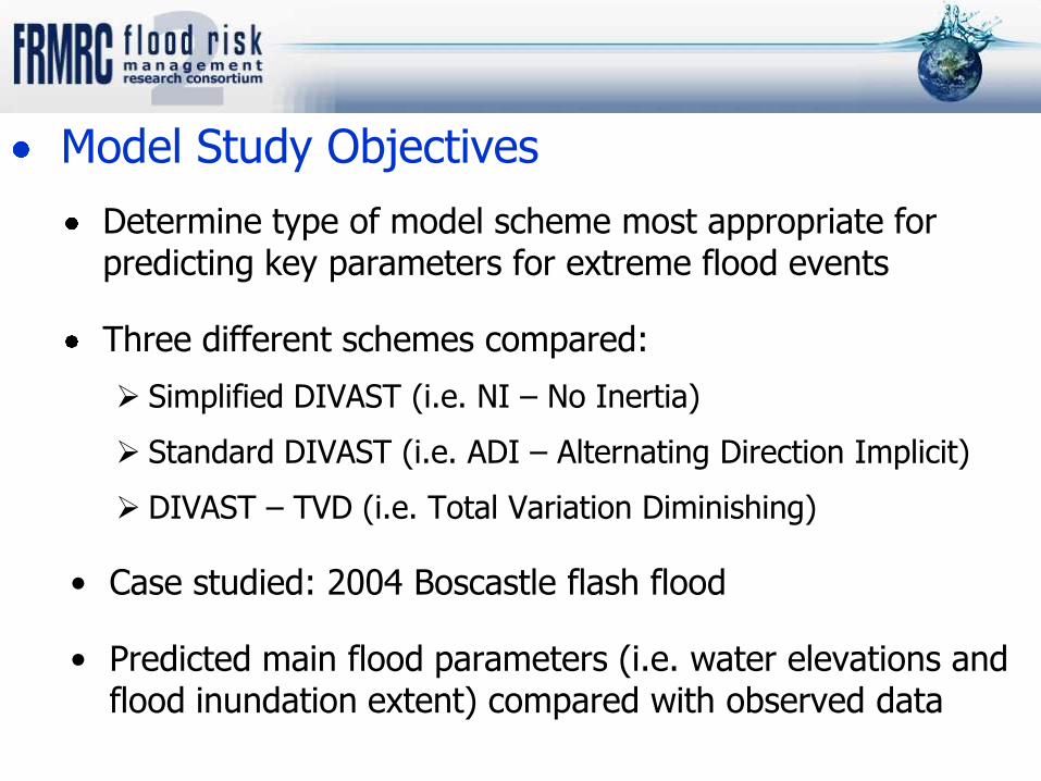
Determine type of model scheme most appropriate for predicting key parameters for extreme flood events
Three different schemes compared:
Simplified DIVAST (i.e. NI – No Inertia)
Standard DIVAST (i.e. ADI – Alternating Direction Implicit)
DIVAST – TVD (i.e. Total Variation Diminishing)
• Case studied: 2004 Boscastle flash flood
• Predicted main flood parameters (i.e. water elevations and flood inundation extent) compared with observed data
Model Study Objectives

Boscastle Study Domain
River Valency

Predicted Flood Simulation (TVD Scheme)

Flood Inundation Extent Predictions
Cases
NI – No Inertia
ADI – Alternating Direction Implicit
TVD – Shock Capturing

Predicted and Measured Water Levels

Models can be extended to include treatment of buildings on floodplains using surface/subsurface models offering
attractive options for flood modelling (e.g. health impact)
For rivers with trans- or supercritical flows, or levee breeches, then need to use more complex models and replicate hydrodynamic processes more accurately
Computational models with shock capturing algorithms provide more accurate predictions of flood elevations
Debris and vehicles can increase flood risk by blocking bridges and culverts to reduce local discharges
Summary

Wrong exit Debris flow problem


Study first undertaken to determine incipient velocity for fully submerged vehicles
Subsequent studies undertaken for partially submerged vehicles based on:
Based on physics derived formulae
Flume experiments based on similarity laws
Parameter determination and formulae validation
Based on incipient velocity for prototype vehicles
Incipient Velocity for Vehicles in Floodwaters

Formula Derivation
Different forces acting on a partially submerged vehicle
FR
FG
FN
U
FD
FG : Effective weight
FD: Drag force
FN : Normal force
FR: Frictional force

2
[ ( )] [ ( )]2f
bd d f c c c c c c f f f
uC a h b a l b h R h
g
2c c cb c f
d d f f
a hu gl R
a C h
(1 )( )f
yu U
h
2f c c
c c f
c f f
h hU gl R
h h
1
1
c
b d d
a
a C a
α, β = Parameters, to be calibrated using flume experiments;
Uc = Incipient velocity for a partially submerged vehicle.
D RF F

Flume Experiments for Vehicle Instability
Experiments conducted in HRC flume Cardiff University. Flume: 15 m long, 1.20 m wide and 1.00 m deep, plastic bed and glass sides
To estimate critical conditions for prototype vehicles - scaled model vehicles used, with 3 similarity laws used to design flume experiments
Partially submerged vehicle test Experimental test flume

Prototype can be analysed from experiments if similarity occurs with: form (geometric), motion (kinematic) and force (dynamic) .
Scale ratios of model experiments
Design of Flume Experiments
Flow and dimensions used typical for Taff

0
0 . 2
0 . 4
0 . 6
0 . 8
1
1 . 2
1 . 4
1 . 6
0 0 . 0 1 0 . 0 2 0 . 0 3 0 . 0 4h ( m )
U(
m/s
)
180°
0°
(a) Ford Focus
Uc (
m/s
)
hf (m)
U
U
0
0.2
0.4
0.6
0.8
1
1.2
1.4
1.6
0.01 0.02 0.03 0.04h (m)
U(m
/s)
180°
0°
(b) Ford Transit
Uc
(m/s
)
hf (m)
U
U
0
0.2
0.4
0.6
0.8
1
1.2
1.4
1.6
1.8
0.01 0.02 0.03 0.04h (m)
U(m
/s)
180°
0°
(c) Volvo XC90
Uc
(m/s
)
hf (m)
U
U
Depth-incipient velocity relationships for partially submerged vehicles

Incipient Velocity for Prototype Vehicles
Incipient velocities for
partially submerged
vehicles in floodwaters
estimated using two
methods: (i) using
model scale ratios, (ii)
computations based
on derived formulae
0.0
1.0
2.0
3.0
4.0
5.0
6.0
0.1 0.2 0.3 0.4 0.5 0.6 0.7hf (m)
Uc
(m/s
)
Eq.(12)(Ford Focus ST)
Eq.(12) (Ford Transit)
Eq.(12)(Volvo XC90)
Eq.(13)(Ford Focus ST)
Eq.(13)(Ford Transit)
Eq.(13)(Volvo XC90)
Ford Focus ST
Ford Transit
Volvo XC90
Comparison between estimated incipient velocities using two different approaches

Assessment of People Safety
Previous studies carried out using two approaches:
Empirical or semi-quantitative criteria Stability analysis validated by experimental data

Instability curves for child and adult in floodwaters
Keller and Mitsch (1992) established balanced forces acting on a flooded person:- buoyancy, weight, frictional resistance and drag due to flow:-
0.5
2 rc
f d
FU
C A
0.0
0.5
1.0
1.5
2.0
2.5
3.0
3.5
4.0
0.0 0.2 0.4 0.6 0.8 1.0 1.2 1.4 1.6 1.8 2.0
h (m)
Uc
(m/s
)
Child
Adult
Fr = restoring force due to friction;
A = submerged area normal to flow;
Cd = drag coefficient .

Similar approach adopted to previous study on incipient velocity for vehicles
Current study for partially submerged people
Formula derivation
Flume experiments following similarity laws
Parameter determination and formula validation
Estimation of incipient velocity for prototype people
Incipient Velocity for People in Floodwaters

Formula Derivation
186 tests undertaken in China using 1:5.54 scale models
Different forces acting on partially submerged person
FG : Effective weight
FD: Drag force Fb: Buoyancy force
FN : Normal force
FR: Frictional force
O
y
x
ufh
dL
gL
NF
DF
GF
toppling
u
Fb
y
x
(b) (a)

1 12 22 2
( ) cos sin ( )( )f p
p
p f f p f p
h m a bU a m b
h h h h h( )
0Gy gy Gx gx D dF L F L F L
Critical condition for toppling instability, given by moment
around pivot point O :
Giving for velocity v. depth:-:
where: α, γ = coefficients (see paper), mp = body mass,
hp = body height, hf = flow depth,
a1,a2,b1,b2 = body shape coefficients

0.2
0.3
0.4
0.5
0.6
0.7
0.8
0.9
1.0
1.1
1.2
0.2 0.4 0.6 0.8 1 1.2hf (m)
Uc(
m/s
)
Flat ground(Exp.)
Flat ground(Cal.)
1:50 slope(Exp.)
1:25 slope(Exp.)
1:25 slope(Cal.)
1:25 slope(Cal.)
0.2
0.3
0.4
0.5
0.6
0.7
0.8
0.9
1.0
1.1
1.2
0.2 0.4 0.6 0.8 1.0 1.2hf (m)
Uc
(m/s
)
Flat ground
Slope 1:50
Slope 1:25
(a) (b)
Scaled Incipient Velocity vs. Depth
Adult Child

Empirical or Semi-quantitative Criteria
Defra (2003) in UK use simple method to assess flood hazard based on velocity, depth and debris:
HR = flood hazard rating;
H = depth of flooding (m);
U = velocity of floodwaters (m/s);
DF = debris factor (= 0, 1, 2 varies
with probability that debris will
lead to greater hazard)
( 1.5)HR h U DF

Determination of Hazard Degree
U = depth-averaged velocity in a cell (m/s); h = flow depth in a cell (m); Uc = critical velocity for depth (h) for vehicle or people(m/s);
HD = Hazard degree for vehicle or people in floodwaters
Safe if HD=0, Dangerous if HD =1.0
HD=Min(1.0, U/Uc)
Expression used to determine degree of hazard:-
Incipient velocity formula from our studies used to assess vehicle and people safety

Comparison of Hazard Formulae

Model Application
1. Glasgow flood in the UK
2. Boscastle flood in the UK

Map of a small urban area in Glasgow
0
2
4
6
8
10
12
0 600 1200 1800 2400 3000 3600
Time(s)
Dis
charg
e(m
3/s
)
Point X0 = Inflowing location
Points X1-X4= Comparison sites
Qmax=10 m3/s Glasgow

Predicted maximum water depth distribution
Predicted maximum velocity distribution
0.1 0.2 0.3 0.4 0.5 0.6 0.7 0.8 0.9 1 1.1 1.2
Maximum water depth (m)
Frame 001 01 Dec 2009 MaximumZ/U/SF

Distributions of hazard degree for vehicles: (a) Pajero; (b) MiniCooper
(a) (b)
Distributions of hazard degree for people: (a) Children; (b) Adults
(a) (b)

Boscastle Flood
Water depths on streets over 2 m, with high velocities transporting debris and cars
Over 100 vehicles washed away, but no fatalities
Valency
Jordan
Car Park
P1
P2
P3
P4

209600 209700 209800 209900 210000 210100 21020091150
91200
91250
91300
91350
91400
91450
91500
91550
91600
Frame 001 29 Nov 2009 MaximumZ/U/SF
Domain showing upstream and downstream boundaries
1
2
3
4
5
6
7
8
0 100 200 300 400 500
Discharge (m3/s)
Sta
ge(m
)
0
20
40
60
80
100
120
140
160
180
0 2 4 6 8 10
Time (h)
Dis
char
ge(m
3/s
)
Rating curve Discharge hydrograph
Outlet
Inlet
Flood Frequency
0.25%=400 Years

Distribution of water depth and velocity at Qpk
209600 209700 209800 209900 210000 210100 21020091150
91200
91250
91300
91350
91400
91450
91500
91550
91600
0.1 0.2 0.5 1 1.5 2 2.5 3 3.5 4Depth (m)4m/s
CS
2
CS
1
Frame 001 29 Nov 2009 Hydrodynamic Results in Nodes
CS2 CS1
Distance for the right side (m)
Bed
or
Wat
erL
evel
(m)
Vel
oci
ty(m
/s)
0 20 40 60 80 100 120
0
6
12
18
24
30
36
0
2
4
6
8
10
12
Bed level
Water level
Velocity
Frame 001 01 Dec 2009 HYD-VP Hazard Degree
Distance from the right side (m)
Bed
or
Wat
erL
evel
(m)
Vel
oci
ty(m
/s)
0 10 20 30 40 50 60 70 80 90
0
3
6
9
12
15
18
0
2
4
6
8
10
12Bed level
Water level
Velocity
Frame 001 01 Dec 2009 HYD-VP Hazard Degree

209600 209700 209800 209900 210000 210100 21020091150
91200
91250
91300
91350
91400
91450
91500
91550
91600
0.01 0.1 0.2 0.4 0.8 1.2 1.6 2 2.4 2.8 3.2 3.6 4Maximum depth(m)
Frame 001 29 Nov 2009 MaximumZ/U/SF
209600 209700 209800 209900 210000 210100 21020091150
91200
91250
91300
91350
91400
91450
91500
91550
91600
0.4 0.8 1.2 1.6 2 2.4 2.8 3.2 3.6 4Maximum velocity (m/s)
Frame 001 29 Nov 2009 MaximumZ/U/SF
Maximum water depth
Maximum velocity

Comparison between predicted peak levels and flood tracks
4
6
8
10
12
14
16
18
20
4 6 8 10 12 14 16 18 20
Observed flood tracks (m)
Pre
dic
ted
ma
xim
um
le
ve
l (m
)

Hazard degree for vehicles: (a) Pajero; (b) MiniCooper
209600 209700 209800 209900 210000 210100 21020091150
91200
91250
91300
91350
91400
91450
91500
91550
91600
0.1 0.2 0.3 0.4 0.5 0.6 0.7 0.8 0.9 1Hazard degree of Mini CPs
Frame 001 29 Nov 2009 MaximumZ/U/SF
(b) Car Park
209600 209700 209800 209900 210000 210100 21020091150
91200
91250
91300
91350
91400
91450
91500
91550
91600
0.1 0.2 0.3 0.4 0.5 0.6 0.7 0.8 0.9 1Hazard degree of Pajero JPs
Frame 001 29 Nov 2009 MaximumZ/U/SF
(a) Car Park

Hazard degree for people: (a) Children; (b) Adults
209600 209700 209800 209900 210000 210100 21020091150
91200
91250
91300
91350
91400
91450
91500
91550
91600
0.1 0.2 0.3 0.4 0.5 0.6 0.7 0.8 0.9 1Hazard degree of Children
Frame 001 29 Nov 2009 MaximumZ/U/SF
209600 209700 209800 209900 210000 210100 21020091150
91200
91250
91300
91350
91400
91450
91500
91550
91600
0.1 0.2 0.3 0.4 0.5 0.6 0.7 0.8 0.9 1Hazard degree of Adults
Frame 001 29 Nov 2009 MaximumZ/U/SF
(a)
(b)
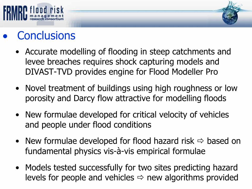
Conclusions
• Accurate modelling of flooding in steep catchments and levee breaches requires shock capturing models and DIVAST-TVD provides engine for Flood Modeller Pro
• Novel treatment of buildings using high roughness or low porosity and Darcy flow attractive for modelling floods
• New formulae developed for critical velocity of vehicles and people under flood conditions
• New formulae developed for flood hazard risk based on
fundamental physics vis-à-vis empirical formulae
• Models tested successfully for two sites predicting hazard levels for people and vehicles new algorithms provided