Modelling diesel engines with a variable-geometry …430022/FULLTEXT02.pdfModelling diesel engines with a variable-geometry turbocharger and exhaust gas recirculation by optimization

Modelling diesel engines with a variable-

geometry turbocharger and exhaust gas

recirculation by optimization of model

parameters for capturing non-linear system

dynamics

Johan Wahlström and Lars Eriksson

Linköping University Post Print

N.B.: When citing this work, cite the original article.

Original Publication:

Johan Wahlström and Lars Eriksson, Modelling diesel engines with a variable-geometry

turbocharger and exhaust gas recirculation by optimization of model parameters for capturing

non-linear system dynamics, 2011, Proceedings of the Institution of mechanical engineers.

Part D, journal of automobile engineering, (225), 7, 960-986.

http://dx.doi.org/10.1177/0954407011398177

Copyright: Professional Engineering Publishing (Institution of Mechanical Engineers)

http://journals.pepublishing.com/

Postprint available at: Linköping University Electronic Press

http://urn.kb.se/resolve?urn=urn:nbn:se:liu:diva-69615

http://dx.doi.org/10.1177/0954407011398177

http://journals.pepublishing.com/

http://urn.kb.se/resolve?urn=urn:nbn:se:liu:diva-69615

Modelling diesel engines with a variable-geometryturbocharger and exhaust gas recirculation byoptimization of model parameters for capturingnon-linear system dynamicsJ Wahlstrom* and L Eriksson

Department of Electrical Engineering, Linkoping University, Linkoping, Sweden

The manuscript was received on 12 February 2010 and was accepted after revision for publication on 4 January 2011.

DOI: 10.1177/0954407011398177

Abstract: A mean-value model of a diesel engine with a variable-geometry turbocharger(VGT) and exhaust gas recirculation (EGR) is developed, parameterized, and validated. Theintended model applications are system analysis, simulation, and development of model-based control systems. The goal is to construct a model that describes the gas flow dynamicsincluding the dynamics in the manifold pressures, turbocharger, EGR, and actuators with fewstates in order to obtain short simulation times. An investigation of model complexity anddescriptive capabilities is performed, resulting in a model that has only eight states. ASimulink implementation including a complete set of parameters of the model are availablefor download. To tune and validate the model, stationary and dynamic measurements havebeen performed in an engine laboratory. All the model parameters are estimated automati-cally using weighted least-squares optimization and it is shown that it is important to tuneboth the submodels and the complete model and not only the submodels or not only thecomplete model. In static and dynamic validations of the entire model, it is shown that themean relative errors are 5.8 per cent or lower for all measured variables. The validations alsoshow that the proposed model captures the system properties that are important for controldesign, i.e. a non-minimum phase behaviour in the channel EGR valve to the intake manifoldpressure and a non-minimum phase behaviour, an overshoot, and a sign reversal in the VGTto the compressor mass flow channel, as well as couplings between channels.

Keywords: diesel engines, modelling, variable-geometry turbocharger, exhaust gas

recirculation, non-linear system

1 INTRODUCTION

Legislated emission limits for heavy-duty trucks are

constantly being reduced. To fulfil the requirements,

technologies such as exhaust gas recirculation (EGR)

systems and variable-geometry turbochargers (VGTs)

have been introduced. The primary emission reduc-

tion mechanisms utilized to control the emissions

are that nitrogen oxides NOx can be reduced by

increasing the intake manifold EGR fraction xegr and

smoke can be reduced by increasing the oxygen-

to-fuel ratio lO [1]. However, xegr and lO depend in

complicated ways on the actuation of the EGR and

VGT. It is therefore necessary to have coordinated

control of the EGR and VGT to reach the legislated

emission limits in NOx and smoke. When developing

and validating a controller for this system, it is desir-

able to have a model that describes the system

dynamics and the non-linear effects that are impor-

tant for gas flow control. These important properties

*Corresponding author: Department of Electrical Engineering,

Linkoping University, Linkoping 58183, Sweden.

email: [email protected]

960

Proc. IMechE Vol. 225 Part D: J. Automobile Engineering

have been described in references [2] to [4], showing

that this system has non-minimum phase beha-

viours, overshoots, and sign reversals. Therefore, the

objective of this paper is to construct a mean-value

diesel engine model, from the actuator input to the

system output, that captures these properties. The

intended applications of the model are system analy-

sis, simulation, and development of model-based

control systems. The model will describe the dynam-

ics in the manifold pressures, turbocharger, EGR,

and actuators with few states in order to obtain short

simulation times.

A successful modelling is the combined result

of experience and systematic analysis of a problem

and balances model complexity with descriptive

capability. This paper collects and summarizes

the knowledge gained over several years about

models for EGR and/or VGT systems and presents

a complete and validated model for such an

engine. The main contributions in this paper are

as follows.

1. An analysis is given of how model assumptions

influence the system dynamics highlighting the

balance between the model complexity and the

dynamics.

2. It is shown that inclusion of the temperature

states and the pressure drop over the intercooler

have only minor effects on the dynamic behav-

iour and that they have a minor influence on

the model quality.

3. Based on the analysis a model structure is pro-

posed, where the emphasis is on using a small

set of states. The essence of the system is cap-

tured by five states related to gas flows. In addi-

tion, actuator models are necessary in many

applications and here the experimental results

show that three states are needed.

4. A tuning method for the model parameters,

consisting of initialization methods for each sub-

model and least-squares optimization, is de-

scribed. In system identification and in tuning of

mean-value engine models, it is common to use

either the submodels or the complete model in

this optimization. However, here it is shown that

it is important to use both the submodels and

the complete model in the optimization to

reduce errors in the complete model.

5. The cylinder-out temperature is modelled using

a fixed-point iteration and it is shown that it is

sufficient to use one iteration in this iterative

process to achieve an accuracy of 0.15 per cent.

6. A survey of diesel engine model components is

provided, summarizing related work and its

relation to the proposed model.

A key feature of the resulting model is its

component-based structure with parameterized

functions for describing the component perfor-

mance. This reduces the dependence on maps and

their associated performance. The model is imple-

mented as a Simulink file complemented by a

parameter file and is available as a companion to

this paper [5]; this implementation is provided for

download or by contacting the authors. More

details about the provided model are given in

Appendix 3. Further, the model reported here has

received widespread acceptance in industry and is

used in both industrial and academic applications

(see, for example, references [6] to [15]).

1.1 Outline

A survey of different models is presented in section

2. This section also briefly describes the structure of

the proposed model as well as the tuning and the

validation. Model equations are described for each

submodel in sections 3 to 7. Section 8 describes the

optimization of the model parameters and the

model validation. The goal is also to investigate

whether the proposed model can be improved with

model extensions in section 9.

2 SURVEY AND MODEL SUMMARY

The proposed model is a mean-value engine model

that uses filling and emptying concepts for the mani-

folds [1, 16, 17]. Several mean-value models with dif-

ferent selections of states and complexities have

been published for diesel engines with EGR and

VGT. A third-order model that describes the intake

and exhaust manifold pressure and turbocharger

dynamics has been developed in reference [18]. The

model in reference [3] has six states describing the

intake and exhaust manifold pressures, the tempera-

ture dynamics, and the turbocharger and compressor

mass flow dynamics. A seventh-order model that

describes the intake and exhaust manifold pressure,

temperature, air-mass fraction dynamics, and turbo-

charger dynamics was proposed in reference [19].

These dynamics are also described by the seventh-

order models in references [2], [4], and [18], where

the burned gas fraction is used instead of the air-

mass fraction in the manifolds. Another model that

describes these dynamics is the ninth-order model

in reference [20] which also has two states for the

actuator dynamics.

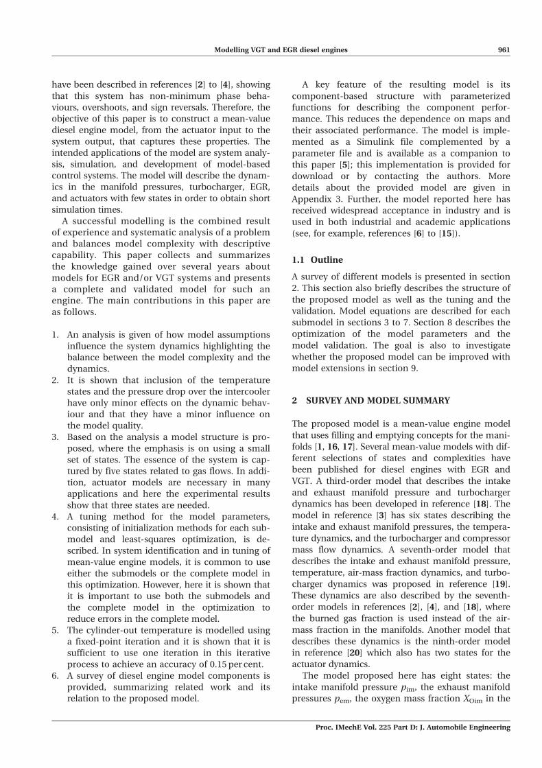
The model proposed here has eight states: the

intake manifold pressure pim, the exhaust manifold

pressures pem, the oxygen mass fraction XOim in the

Modelling VGT and EGR diesel engines 961


intake manifold, the oxygen mass fraction XOem in

the exhaust manifold, the turbocharger speed vt,

and three states (~uegr1, ~uegr2, and ~uvgt) describing

the actuator dynamics for the two control signals.

These states are collected in a state vector x accord-

ing to

x = (pim pem XOim XOem vt ~uegr1 ~uegr2 ~uvgt)T (1)

Descriptions of the notation and the variables

can be found in the Appendices, and the structure

of the model can be seen in Fig. 1.

The states pim, pem, and vt describe the main

dynamics and the most important system proper-

ties, such as the non-minimum phase behaviours,

overshoots, and sign reversals. In order to model

the dynamics in the oxygen-to-fuel ratio lO, the

states XOim and XOem are used. Finally, the states~uegr1, ~uegr2, and ~uvgt describe the actuator dynamics

where the EGR valve actuator model has two states~uegr1 and ~uegr2 in order to describe an overshoot in

the actuator.

Many models in the literature, which have

approximately the same complexities as the model

proposed here, use three states for each control

volume in order to describe the temperature

dynamics [2, 18, 20]. However, the model proposed

here uses only two states for each manifold: pres-

sure and oxygen mass fraction. Model extensions

are investigated in section 9.1, showing that inclu-

sion of the temperature states has only minor

effects on the dynamic behaviour. Furthermore, the

pressure drop over the intercooler is not modelled

since this pressure drop has only small effects on

the dynamic behaviour. However, this pressure

drop has large effects on the stationary values, but

these effects do not improve the complete engine

model (see section 9.2).

2.1 Model structure

It is important that the model can be utilized both

for different vehicles and for engine testing and cal-

ibration. In these situations the engine operation is

defined by the rotational speed ne, e.g. given as an

input from a drive cycle, and therefore it is natural

to parameterize the model using the engine speed.

The resulting model is thus expressed in state space

form as

_x = f (x, u, ne) (2)

where the engine speed ne is considered as a mea-

sured disturbance, and u is the control input vector

given by

u = (ud uegr uvgt)T (3)

which contains a mass ud of injected fuel, EGR

valve position uegr, and VGT actuator position uvgt.

The EGR valve is closed when uegr = 0 per cent and

open when uegr = 100 per cent. The VGT is closed

when uvgt = 0 per cent and open when uvgt = 100

per cent.

2.2 Measurements

To tune and validate the model, stationary and

dynamic measurements were performed in an

engine laboratory at Scania CV AB, and these are

described below. Furthermore, in Appendix 2 the

sensor dynamics are investigated showing that the

dynamics visible in the experimental data are due

to the system dynamics, this is because the sensors

are much faster than the system dynamics.

2.2.1 Stationary measurements

The stationary data consist of measurements in sta-

tionary conditions at 82 operating points, which are

scattered over a large operating region covering dif-

ferent loads, speeds, and VGT and EGR positions.

These 82 operating points also include the

European stationary cycle at 13 operating points.

The variables that were measured during station-

ary measurements are given later in Table 5 in

Appendix 2.

Fig. 1 A model structure of the diesel engine. It hasthree control inputs and five main states relatedto the engine (pim, pem, XOim, XOem, and vt). Inaddition, there are three states for actuatordynamics (~uegr1, ~uegr2, and ~uvgt)

962 J Wahlstrom and L Eriksson


All the stationary measurements are used for

tuning the parameters in static models. The static

models are then validated using dynamic measure-

ments.

2.2.2 Dynamic measurements

The dynamic data consist of measurements in

dynamic conditions with steps in the VGT control

signal, EGR control signal, and fuel injection at sev-

eral different operating points according to Table 1.

The steps in the VGT position and EGR valve are

performed for the data sets A to H, J, and Q to U,

and the steps in fuel injection are performed in the

data sets I and V. The data set J is used for tuning

the dynamic actuator models and the data sets B, C,

and I are used for tuning the dynamic models in

the manifolds, in the turbocharger, and in the

engine torque respectively. Further, the data sets A

to I are used for tuning the static models, the data

sets A and D to I are used for validation of the

dynamic models, and the data sets Q to V are used

for validation of both the static and the dynamic

models. The main difference between the tuning

and validation data is that they have different

engine loads and thus different flows and pressures.

The dynamic measurements are limited in the

sample rate with a sample frequency of 1 Hz for the

data sets A, D to G, and R to V, 10 Hz for the data

set I, and 100 Hz for the data sets B, C, H, J, and Q.

This means that the data sets A, D to G, I, and R to

V, do not capture the fastest dynamics in the

system, while the data sets B, C, H, J, and Q do.

Further, the data sets B, C, H, J, and Q were mea-

sured 3.5 years after the data sets A, D to G, I and R

to V and the stationary data. The variables that

were measured during dynamic measurements can

be seen later in Table 6 in Appendix 2.

2.3 Parameter estimation and validation

The model parameters are estimated in five steps.

First, the static parameters are initialized using

least-squares optimization for each submodel in

section 3 to 6 and data from stationary measure-

ments. Second, the actuator parameters are esti-

mated using least-squares optimization for the

actuator models and using the dynamic measure-

ments in the data set J in Table 1. Third, the mani-

fold volumes and the turbocharger inertia and,

fourth, the time constant for the engine torque are

estimated using least-squares optimization for the

complete model and using data from the dynamic

measurements in the data sets B, C, and I in

Table 1. Fifth, the static parameters are finally esti-

mated using least-squares optimization for each

submodel and for the complete model and using

data from both the stationary and the dynamic

measurements. The dynamic measurements used

are the data sets A to I in Table 1. In the fifth step

the static parameters are initialized using the

method in the first step.

Systematic tuning methods for each parameter

are described in detail in sections 3 to 6, and sec-

tion 8.1. In section 8.2 it is shown that is important

to use both the submodels and the complete model

in the tuning method to reduce errors in the com-

plete model. Since the proposed tuning methods

are systematic and general, it is straightforward to

re-create the values of the model parameters and to

apply the tuning methods to different diesel engines

with EGR and VGT.

Because there were only a few stationary mea-

surements, both the static and the dynamic models

are validated by simulating the complete model and

comparing it with the dynamic measurements Q to

V in Table 1. The dynamic models are also validated

using the dynamic measurements A and D to I in

Table. 1.

2.4 Relative error

Relative errors are calculated and used to evaluate

the tuning and the validation of the model. Rela-

tive errors for stationary measurements between

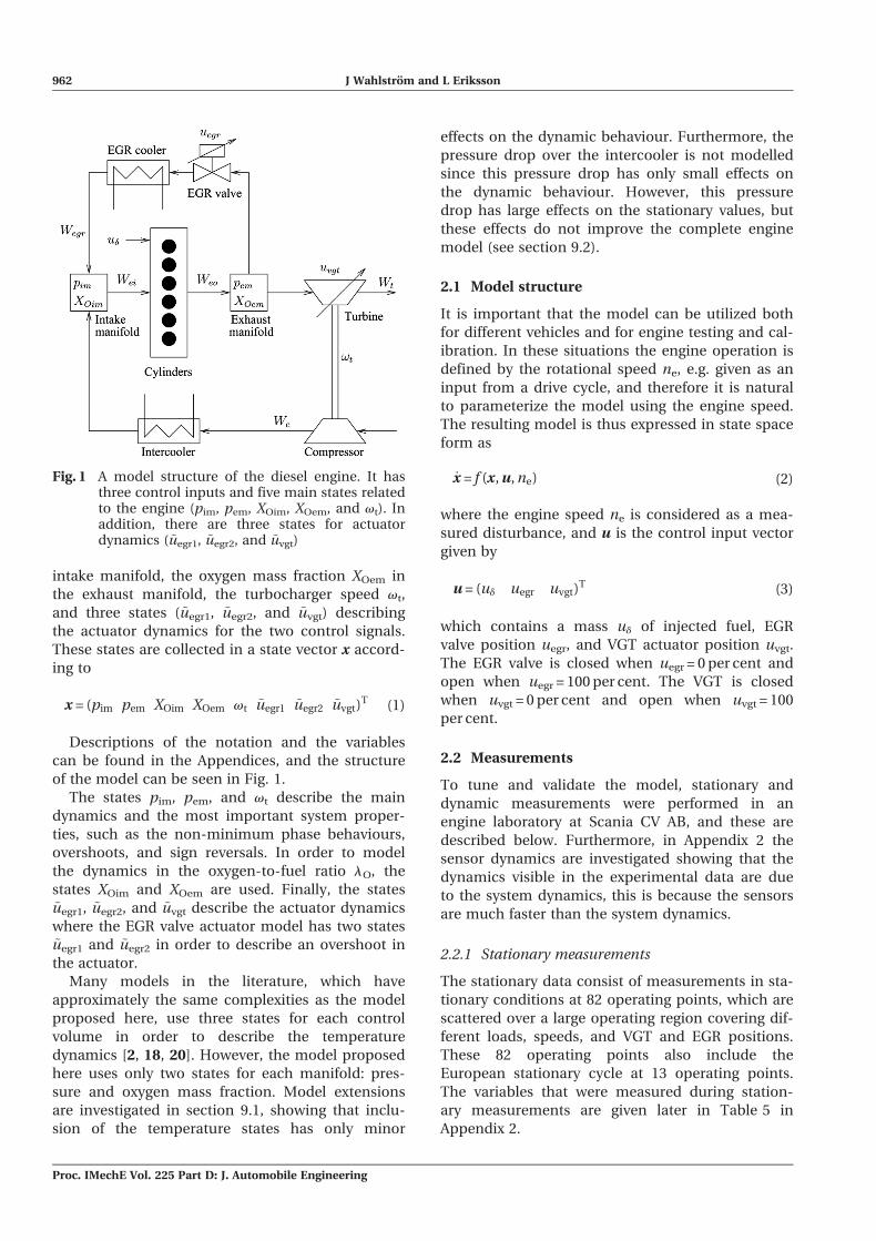
Table 1 Dynamic tuning and validation data that consist of steps in the VGT position, EGR valve, and fuel injec-

tion. The data sets B, C, I, and J are used for tuning of dynamic models, the data sets A to I are used for

tuning the static models, the data sets A and D to I are used for validating the dynamic models, and the

data sets Q to V are used for validating both the static and the dynamic models

Data set

VGT and EGR steps ud steps VGT and EGR steps

A B Q C R D S E T F U G H I V J

Speed (r/min) 1200 1200 1200 1200 1200 1200 1500 1500 1500 1900 1900 1900 1900 1500 1500 –Load (%) 25 40 40 50 50 75 25 50 75 25 50 75 100 – – –Number of steps 77 23 12 2 77 77 77 77 77 77 77 55 1 7 28 48Sample frequency (Hz) 1 100 100 100 1 1 1 1 1 1 1 1 100 10 1 100



a measured variable ymeas,stat and a modelled vari-

able ymod,stat are calculated as

Stationary relative error(i)

=ymeas,stat(i)� ymod,stat(i)

1=NPN

i = 1 ymeas,stat(i) (4)

where i is an operating point. Relative errors for

dynamic measurements between a measured vari-

able ymeas,dyn and a modelled variable ymod,dyn are

calculated as

Dynamic relative error(j)

=ymeas,dyn(j)� ymod,dyn(j)

1=NPN

i = 1 ymeas,stat(i) (5)

where j is a time sample. In order to make a fair

comparison between these relative errors, both the

stationary relative error and the dynamic relative

error have the same stationary measurement in the

denominator and the mean value of this stationary

measurement is calculated in order to avoid large

relative errors when ymeas,stat is small.

3 MANIFOLDS

The intake and exhaust manifolds are modelled as

dynamic systems with two states each, and these

are pressure and oxygen mass fraction. The stan-

dard isothermal model [1], which is based upon

mass conservation, the ideal-gas law, and the fact

that the manifold temperature is constant or varies

slowly, gives the differential equations for the mani-

fold pressures as

d

dtpim =

Ra Tim

VimWc + Wegr �Wei

� �d

dtpem =

Re Tem

VemWeo �Wt �Wegr

� �(6)

There are two sets of thermodynamic properties:

air has the ideal-gas constant Ra and the specific

heat capacity ratio ga, exhaust gas has the ideal-gas

constant Re and the specific heat capacity ratio ge.

The intake manifold temperature Tim is assumed to

be constant and equal to the cooling temperature in

the intercooler, the exhaust manifold temperature

Tem will be described in section 4.2, and Vim and

Vem are the manifold volumes. The mass flows Wc,

Wegr, Wei, Weo, and Wt will be described in sections

4 to 6.

The EGR fraction in the intake manifold is calcu-

lated as

xegr =Wegr

Wc + Wegr(7)

Note that the EGR gas also contains oxygen which

affects the oxygen-to-fuel ratio in the cylinder. This

effect is considered by modelling the oxygen con-

centrations XOim and XOem in the control volumes.

These concentrations are defined in the same way

as in reference [4] according to

XOim =mOim

mtotim, XOem =

mOem

mtotem(8)

where mOim and mOem are the oxygen masses in the

intake manifold and exhaust manifold respectively,

and mtotim and mtotem are the total masses in the

intake manifold and exhaust manifolds respectively.

Differentiating XOim and XOem and using mass con-

servation [4] give the differential equations

d

dtXOim =

Ra Tim

pim Vim(XOem � XOim)Wegr

�+ (XOc � XOim)WcÞ

d

dtXOem =

Re Tem

pem VemXOe � XOemð ÞWeo

(9)

where XOc is the constant oxygen concentration

passing through the compressor, i.e. air with

XOc = 23.14 per cent, and XOe is the oxygen concen-

tration in the exhaust gases coming from the engine

cylinders, XOe will be described in section 4.1.

Another way to consider the oxygen in the EGR

gas is to model the burned gas ratio Fx in the con-

trol volume x which is a frequent choice for states

in many papers [2, 18, 20]. The relation between

the oxygen concentration XOx and the burned gas

ratio Fx in the control volume x is

XOx = XOc(1� Fx) (10)

Inserting this relation into equation (9), the dif-

ferential equations in references [2], [18], and [20]

are obtained. Consequently, the states XOx and Fx

are equivalent.

3.1 Manifold volumes

Tuning parameters. The tuning parameters are the

intake manifold volumes Vim and the exhaust mani-

fold volume Vem.Tuning method. The tuning parameters Vim and

Vem are determined using least-squares optimiza-

tion for the complete model and using data from



the dynamic measurements in the data set B and C

in Table 1, see section 8.1 for more details.

4 CYLINDER

Three submodels describe the behaviour of the cyl-

inder; these are as follows:

(a) a mass flow model that describes the gas and

fuel flows that enter and leave the cylinder, the

oxygen-to-fuel ratio, and the oxygen concen-

tration out from the cylinder;

(b) a model of the exhaust manifold temperature;

(c) an engine torque model.

4.1 Cylinder flow

The total mass flow Wei from the intake manifold

into the cylinders is modelled using the volumetric

efficiency hvol [1] and is given by

Wei =hvol pim ne Vd

120Ra Tim(11)

where pim and Tim are the pressure and temperature

respectively in the intake manifold, ne is the engine

speed, and Vd is the displaced volume. The volu-

metric efficiency is in its turn modelled as

hvol = cvol1ffiffiffiffiffiffiffiffipimp

+ cvol2

ffiffiffiffiffine

p+ cvol3 (12)

The fuel mass flow Wf into the cylinders is con-

trolled by ud, which gives the injected mass of fuel

in milligrams per cycle and cylinder as

Wf =10�6

120ud ne ncyl (13)

where ncyl is the number of cylinders. The mass

flow Weo out from the cylinder is given by the mass

balance as

Weo = Wf + Wei (14)

The oxygen-to-fuel ratio lO in the cylinder is

defined as

lO =Wei XOim

Wf (O=F)s(15)

where (O=F)s is the stoichiometric ratio of the

oxygen mass to the fuel mass. The oxygen-to-fuel

ratio is equivalent to the air-to-fuel ratio which is

a common choice of performance variable in the lit-

erature [18, 20–22].

During the combustion, the oxygen is burned in

the presence of fuel. In diesel engines, lO . 1 to

avoid smoke. Therefore, it is assumed that lO . 1

and the oxygen concentration out from the cylinder

can then be calculated as the unburned oxygen

fraction

XOe =Wei XOim �Wf (O=F)s

Weo(16)

Tuning parameters. The tuning parameters are

the volumetric efficiency constants cvol1, cvol2, cvol3.Initialization method. The tuning parameters

cvol1, cvol2, and cvol3 are initialized by solving a

linear least-squares problem that minimizes

(Wei 2 Wei,meas)2 with cvol1, cvol2, and cvol3 as the opti-

mization variables. The variable Wei is the model in

equations (11) and (12) and Wei,meas is calculated

from stationary measurements as Wei,meas = Wc/

(1 2 xegr). Stationary measurements are used as

inputs to the model during the tuning. The result of

the initialization is that the cylinder mass flow

model has a mean absolute relative error of 0.9 per

cent and a maximum absolute relative error of

2.5 per cent. The parameters are then tuned accord-

ing to the method in section 8.1.

4.2 Exhaust manifold temperature

The exhaust manifold temperature model consists

of a model for the cylinder-out temperature and

a model for the heat losses in the exhaust pipes.

4.2.1 Cylinder-out temperature

The cylinder-out temperature Te is modelled in the

same way as in reference [23]. This approach is

based upon ideal-gas Seliger cycle (or limited pres-

sure cycle [1]) calculations that give the cylinder-

out temperature as

Te = hsc P1�1=gae r1�ga

c x1=ga�1p

3 qin1� xcv

cpa+

xcv

cV a

� �+ T1 rga�1

c

� �(17)

where hsc is a compensation factor for non-ideal

cycles and xcv the ratio of fuel consumed during

constant-volume combustion. The rest of the fuel,

i.e. (1 2 xcv) is used during constant-pressure com-

bustion. The model (17) also includes the following

six components: the pressure ratio over the cylinder

given by



Pe =pem

pim(18)

the pressure ratio between point 3 (after combus-

tion) and point 2 (before combustion) in the Seliger

cycle given by

xp =p3

p2= 1 +

qin xcv

cV a T1 rga�1c

(19)

the specific energy contents of the charge given by

qin =Wf qHV

Wei + Wf1� xrð Þ (20)

the temperature when the inlet valve closes after

the intake stroke and mixing given by

T1 = xr Te + 1� xrð ÞTim (21)

the residual gas fraction given by

xr =P1=ga

e x�1=gap

rc xv

(22)

and the volume ratio between point 3 (after com-

bustion) and point 2 (before combustion) in the

Seliger cycle given by

xv =v3

v2= 1 +

qin 1� xcvð Þcpa ðqin xcv=cV aÞ+ T1 r

ga�1c

h i(23)

4.2.2 Solution to the cylinder-out temperature

Since the equations above are non-linear and

depend on each other, the cylinder-out temperature

is calculated numerically using a fixed-point itera-

tion which starts with the initial values xr,0 and T1,0.

Then the equations

qin, k + 1 =Wf qHV

Wei + Wf1� xr, kð Þ

xp, k + 1 = 1 +qin, k + 1 xcv

cV a T1, k rga�1c

xv, k + 1 = 1 +qin, k + 1 1� xcvð Þ

cpa ½qin, k + 1 xcv=cV a�+ T1, k rga�1c

� �

xr, k + 1 =P1=ga

e x�1=ga

p, k + 1

rc xv, k + 1

Te, k + 1 = hsc P1�1=gae r1�ga

c x1=ga�1p, k + 1

3 qin, k + 11� xcv

cpa+

xcv

cV a

� �+ T1, k rga�1

c

� �T1, k + 1 = xr, k + 1 Te, k + 1 + 1� xr, k + 1ð ÞTim

(24)

are applied in each iteration k. In each sample

during the simulation, the initial values xr,0 and T1,0

are set to the solutions of xr and T1 from the previ-

ous sample.

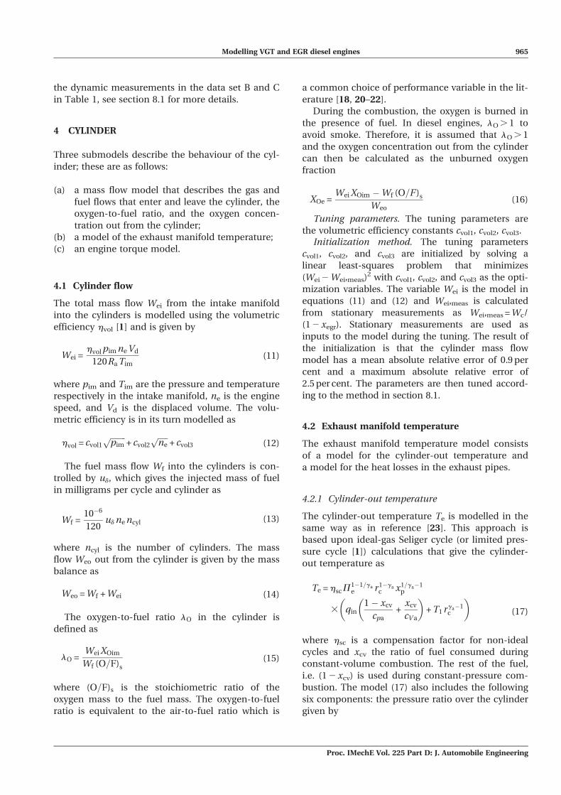
4.2.3 Approximating the solution to thecylinder-out temperature

A simulation of the complete engine model during

the European transient cycle in Fig. 2 shows that it

is sufficient to use one iteration in the iterative pro-

cess (24). This is shown by comparing the solution

from one iteration with one solution that has suf-

ficiently many iterations to give a solution with

0.01 per cent accuracy. The maximum absolute rela-

tive error of the solution from one iteration (com-

pared with the solution with 0.01 per cent accuracy)

is 0.15 per cent. This error is small because the

fixed-point iteration (24) has initial values that are

close to the solution. Consequently, when using this

method in a simulation, it is sufficient to use one

iteration in this model since the mean absolute rel-

ative error of the exhaust manifold temperature

model compared with measurements is 1.7 per cent.

4.2.4 Heat losses in the exhaust pipes

The cylinder-out temperature model above does

not describe the exhaust manifold temperature

completely owing to heat losses in the exhaust

pipes between the cylinder and the exhaust mani-

fold. Therefore the next step is to include a sub-

model for these heat losses.

This temperature drop is modelled in the same

way as model 1 presented in reference [24], where

the temperature drop is described as a function of

mass flow out from the cylinder according to

Tem = Tamb + Te � Tambð Þexp�

htot p dpipe lpipe npipe

Weo cpe (25)

where Tamb is the ambient temperature, htot the total

heat transfer coefficient, dpipe the pipe diameter, lpipe

the pipe length and npipe the number of pipes.Tuning parameters. The tuning parameters are

the compensation factor hsc for non-ideal cycles,

the ratio xcv of fuel consumed during constant-

volume combustion, and the total heat transfer

coefficient htot.Initialization method. The tuning parameters hsc,

xcv, and htot are initialized by solving a non-linear

least-squares problem that minimizes (Tem –

Tem,meas)2 with hsc, xcv, and htot as the optimization

variables. The variable Tem is the model in equa-

tions (24) and (25) with stationary measurements as

inputs to the model, and Tem,meas is a stationary



measurement. The result of the initialization is that

the model describes the exhaust manifold tempera-

ture well, with a mean absolute relative error of

1.7 per cent and a maximum absolute relative error

of 5.4 per cent. The parameters are then tuned

according to the method in section 8.1.

4.3 Engine torque

The torque Me produced by the engine is modelled

using three different engine components, namely

the gross indicated torque Mig, the pumping

torque Mp, and the friction torque Mfric [1], accord-

ing to

Me = Mig �Mp �Mfric (26)

The pumping torque is modelled using the intake

and exhaust manifold pressures, according to

Mp =Vd

4ppem � pimð Þ (27)

The gross indicated torque is coupled to the

energy that comes from the fuel according to

Mig =ud 10�6 ncyl qHV hig

4p(28)

Assuming that the engine is always running at

optimal injection timing, the gross indicated effi-

ciency hig is modelled as

hig = higch 1� 1

rgcyl�1c

!(29)

where the parameter higch is estimated from mea-

surements, rc is the compression ratio, and gcyl is

the specific heat capacity ratio for the gas in the

510 512 514 516 518 520 522 524 526 528 530200

400

600

800

1000

1200

1400(a)

(b)

Te [K

]

One iteration0.01 % accuracy

510 512 514 516 518 520 522 524 526 528 530−0.2

−0.15

−0.1

−0.05

0

0.05

0.1

0.15

rel e

rror

[%]

Time [s]

Fig. 2 The cylinder-out temperature Te calculated by simulating the total engine model duringthe complete European transient cycle. This figure shows the part of the European tran-sient cycle which consists of the maximum relative error. (a) The fixed-point iteration (24)is used in two ways: by using one iteration and to obtain 0.01 per cent accuracy. (b)Relative errors between the solutions from one iteration and 0.01 per cent accuracy



cylinder. The friction torque is assumed to be

a quadratic polynomial in engine speed [1] given by

Mfric =Vd

4p105 cfric1 n2

eratio + cfric2 neratio + cfric3

� �(30)

where

neratio =ne

1000(31)


the combustion chamber efficiency higch and the

coefficients cfric1, cfric2, and cfric3 in the polynomial

function for the friction torque.Tuning method. The tuning parameters higch,

cfric1, cfric2, and cfric3 are determined by solving

a linear least-squares problem that minimizes

(Me + Mp 2 Me,meas 2 Mp,meas)2 with the tuning

parameters as the optimization variables. The

model of Me + Mp is obtained by solving equation

(26) for Me + Mp and Me,meas + Mp,meas is calculated

from stationary measurements as Me,meas + Mp,meas =

Me + Vd(pem 2 pim)/(4p). Station-ary measurements

are used as inputs to the model. The result of the

tuning is that the engine torque model has small

absolute relative errors with a mean absolute relative

error of 1.9 per cent and a maximum absolute rela-

tive error of 7.1 per cent.

5 EGR VALVE

The EGR-valve model consists of submodels for the

EGR-valve mass flow and the EGR-valve actuator.

5.1 EGR-valve mass flow

The mass flow through the EGR valve is modelled

as a simplification of a compressible flow restriction

with variable area [1] and with the assumption that

there is no reverse flow when pem\pim. The motive

for this assumption is to construct a simple model.

The model can be extended with reverse flow, but

this increases the complexity of the model since a

reverse-flow model requires mixing of different

temperatures and oxygen fractions in the exhaust

manifold and a change in the temperature and the

gas constant in the EGR mass flow model. However,

pem is smaller than pim only in a small operating

region with low engine speeds, high engine torque,

and half-open to fully open VGT where the engine

almost never operates [9]. In addition, reverse flow

is also avoided during normal operation by closing

the EGR valve at these points.

The mass flow through the restriction is

Wegr =Aegr pem Cegrffiffiffiffiffiffiffiffiffiffiffiffiffiffi

Tem Re

p(32)

where

Cegr =

ffiffiffiffiffiffiffiffiffiffiffiffiffiffiffiffiffiffiffiffiffiffiffiffiffiffiffiffiffiffiffiffiffiffiffiffiffiffiffiffiffiffiffiffiffiffiffiffiffiffiffiffiffi2ge

ge � 1P2=ge

egr �P1 + 1=geegr

� �s(33)

Measurement data show that equation (33) does

not give a sufficiently accurate description of the

EGR flow. Pressure pulsations in the exhaust mani-

fold or the influence of the EGR cooler could be

two different explanations for this phenomenon.

In order to maintain the density influence

(pem=(ffiffiffiffiffiffiffiffiffiffiffiffiffiffiTem Re

p)) in equation (32) and the simplicity

of the model, the function Cegr is instead modelled

as a parabolic function

Cegr = 1� 1�Pegr

1�Pegropt� 1

� �2

(34)

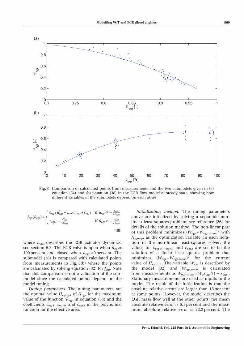
This submodel is compared with calculated points

from measurements of Fig. 3(a) where the points

are calculated by solving equation (32) for Cegr.

Note that this comparison is not a validation of the

submodel since the calculated points depend on

the model tuning.

The pressure ratio Pegr over the valve is limited

when the flow is choked, i.e. when sonic conditions

are reached in the throat, and when 1\pim/pem, i.e.

no back flow can occur, according to

Pegr =

Pegropt if pim

pem\Pegropt

pim

pemif Pegropt<

pim

pem<1

1 if 1\ pim

pem

8><>: (35)

For a compressible flow restriction, the standard

model for Pegropt is

Pegropt =2

ge + 1

� �ge=ge�1

(36)

but the accuracy of the EGR flow model is improved

by replacing the physical value of Pegropt in equa-

tion (36) with a tuning parameter [25].

The effective area

Aegr = Aegrmax fegr(~uegr) (37)

is modelled as a polynomial function of the EGR

valve position ~uegr according to



fegr(~uegr) =cegr1 ~u2

egr + cegr2 ~uegr + cegr3 if ~uegr<� cegr2

2 cegr1

cegr3 �c2

egr2

4 cegr1if ~uegr.� cegr2

2 cegr1

8<:

(38)

where ~uegr describes the EGR actuator dynamics,

see section 5.2. The EGR valve is open when ~uegr =

100 per cent and closed when ~uegr = 0 per cent. The

submodel (38) is compared with calculated points

from measurements in Fig. 3(b) where the points

are calculated by solving equation (32) for fegr. Note

that this comparison is not a validation of the sub-

model since the calculated points depend on the

model tuning.Tuning parameters. The tuning parameters are

the optimal value Pegropt of Pegr for the maximum

value of the function Cegr in equation (34) and the

coefficients cegr1, cegr2, and cegr3 in the polynomial

function for the effective area,

Initialization method. The tuning parameters

above are initialized by solving a separable non-

linear least-squares problem; see reference [26] for

details of the solution method. The non-linear part

of this problem minimizes (Wegr – Wegr,meas)2 with

Pegropt as the optimization variable. In each itera-

tion in the non-linear least-squares solver, the

values for cegr1, cegr2, and cegr3 are set to be the

solution of a linear least-squares problem that

minimizes (Wegr – Wegr,meas)2 for the current

value of Pegropt. The variable Wegr is described by

the model (32) and Wegr,meas is calculated

from measurements as Wegr,meas = Wcxegr/(1 2 xegr).

Stationary measurements are used as inputs to the

model. The result of the initialization is that the

absolute relative errors are larger than 15 per cent

at some points. However, the model describes the

EGR mass flow well at the other points; the mean

absolute relative error is 6.1 per cent and the maxi-

mum absolute relative error is 22.2 per cent. The

0.7 0.75 0.8 0.85 0.9 0.95 10

0.2

0.4

0.6

0.8

1(a)

(b)

Ψeg

r

Πegr

[−]

0 10 20 30 40 50 60 70 80 90 1000

0.2

0.4

0.6

0.8

1

f egr[−

]

uegr

[%]

Fig. 3 Comparison of calculated points from measurements and the two submodels given in (a)equation (34) and (b) equation (38) in the EGR flow model at steady state, showing howdifferent variables in the submodels depend on each other



parameters are then tuned according to the

method in section 8.1.

5.2 EGR-valve actuator

The EGR-valve actuator dynamics are modelled as

a second-order system with an overshoot and

a time delay (Fig. 4). This model consist of a sub-

traction between the two first-order systems with

different gains and time constants according to

~uegr = Kegr ~uegr1 � (Kegr � 1)~uegr2(39)

d

dt~uegr1 =

1

tegr1½uegr(t � tdegr)� ~uegr1� (40)

d

dt~uegr2 =

1

tegr2½uegr(t � tdegr)� ~uegr2� (41)


the time constants tegr1 and tegr2 for the two differ-

ent first-order systems, the time delay tdegr, and a

parameter Kegr that affects the size of the over-

shoot.Tuning method. The tuning parameters above are

determined by solving a non-linear least-squares

problem that minimizes (~uegr – ~uegr,meas)2 with tegr1,

tegr2, tdegr, and Kegr as the optimization variables.

The variable ~uegr is the model in equations (39) to

(41) and ~uegr,meas are dynamic responses in the

dynamic data set J in Table 1. These data consist of

18 steps in the EGR valve position with a step size

of 10 per cent, going from 0 per cent up to 90 per

cent and then back again to 0 per cent with a step

size of 10 per cent. The measurements also consist

of one step with a step size of 30 per cent, one step

with a step size of 75 per cent, three steps with

a step size of 80 per cent, and one step with a step

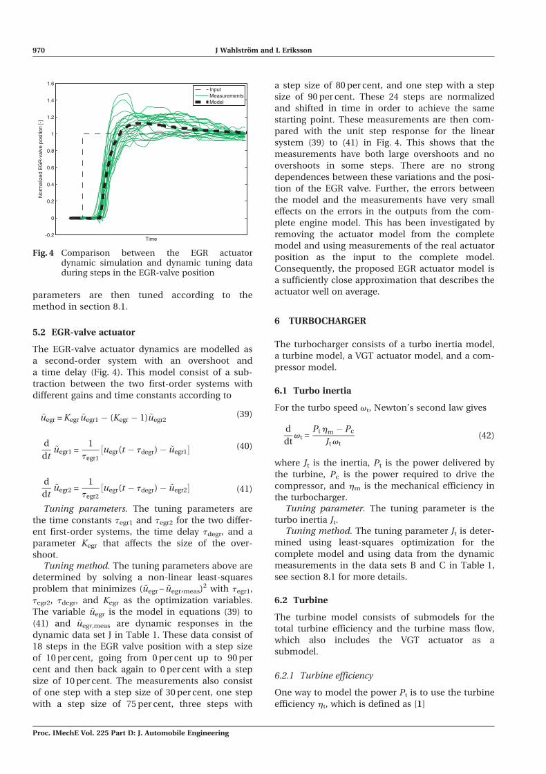
size of 90 per cent. These 24 steps are normalized

and shifted in time in order to achieve the same

starting point. These measurements are then com-

pared with the unit step response for the linear

system (39) to (41) in Fig. 4. This shows that the

measurements have both large overshoots and no

overshoots in some steps. There are no strong

dependences between these variations and the posi-

tion of the EGR valve. Further, the errors between

the model and the measurements have very small

effects on the errors in the outputs from the com-

plete engine model. This has been investigated by

removing the actuator model from the complete

model and using measurements of the real actuator

position as the input to the complete model.

Consequently, the proposed EGR actuator model is

a sufficiently close approximation that describes the

actuator well on average.

6 TURBOCHARGER

The turbocharger consists of a turbo inertia model,

a turbine model, a VGT actuator model, and a com-

pressor model.

6.1 Turbo inertia

For the turbo speed vt, Newton’s second law gives

d

dtvt =

Pt hm � Pc

Jt vt(42)

where Jt is the inertia, Pt is the power delivered by

the turbine, Pc is the power required to drive the

compressor, and hm is the mechanical efficiency in

the turbocharger.Tuning parameter. The tuning parameter is the

turbo inertia Jt.Tuning method. The tuning parameter Jt is deter-

mined using least-squares optimization for the

complete model and using data from the dynamic

measurements in the data sets B and C in Table 1,

see section 8.1 for more details.

6.2 Turbine

The turbine model consists of submodels for the

total turbine efficiency and the turbine mass flow,

which also includes the VGT actuator as a

submodel.

6.2.1 Turbine efficiency

One way to model the power Pt is to use the turbine

efficiency ht, which is defined as [1]

-0.2

0

0.2

0.4

0.6

0.8

1

1.2

1.4

1.6

Nor

mal

ized

EG

R-v

alve

pos

ition

[-]

Time

InputMeasurementsModel

Fig. 4 Comparison between the EGR actuatordynamic simulation and dynamic tuning dataduring steps in the EGR-valve position



ht =Pt

Pt,s=

Tem � Tt

Tem(1�P1�1=get ) (43)

where Tt is the temperature after the turbine, Pt is

the pressure ratio given by

Pt =pes

pem(44)

and Pt,s is the power from the isentropic process

Pt,s = Wt cpe Tem 1�P1�1=get

� �(45)

where Wt is the turbine mass flow. In equation (44),

pes . pamb if there is a restriction (e.g. an after-

treatment system) after the turbine. However, for

this engine there is no restriction after the turbine

and therefore pes = pamb.

In equation (43), it is assumed that there are no

heat losses in the turbine, i.e. it is assumed that

there are no temperature drops between the tem-

peratures Tem and Tt that are due to heat losses.

This assumption leads to errors in ht if equation

(43) is used to calculate ht from measurements. One

way to improve this model is to model these tem-

perature drops, but it is difficult to tune these

models since no measurements of these tempera-

ture drops exist. Another way to improve the model,

that is frequently used in the literature [27], is to

use another efficiency that is approximately equal

to ht. This approximation utilizes the fact that

Pt hm = Pc (46)

at steady state according to equation (42).

Consequently, Pt’Pc at steady state. Using this

approximation in equation (43), another efficiency

htm is obtained as

htm =Pc

Pt,s=

Wc cpa(Tc � Tamb)

Wt cpe Tem 1�P1�1=get

� �(47)

where Tc is the temperature after the compressor

and Wc is the compressor mass flow. The tempera-

ture Tem in equation (47) introduces fewer errors

than the temperature difference Tem – Tt in equation

(43) does because the absolute value of Tem is larger

than the absolute value of Tem – Tt. Consequently,

equation (47) introduces fewer errors than equation

(43) does since equation (47) does not consist of

Tem – Tt. The temperatures Tc and Tamb are low and

they introduce fewer errors than Tem and Tt since

the heat losses in the compressor are comparatively

small. Another advantage of using equation (47) is

that the individual variables Pt and hm in equation

(42) do not have to be modelled. Instead, the prod-

uct Pthm is modelled using equations (46) and (47)

according to

Pt hm = htm Pt,s = htm Wt cpe Tem 1�P1�1=get

� �(48)

Measurements show that htm depends on the blade

speed ratio (BSR) as a parabolic function [28],

according to

htm = htm, max � cm(BSR� BSRopt)2 (49)

The BSR is the ratio of the turbine blade tip speed

to the speed which a gas reaches when expanded

isentropically at the given pressure ratio Pt; the BSR

is given by

BSR =Rt vtffiffiffiffiffiffiffiffiffiffiffiffiffiffiffiffiffiffiffiffiffiffiffiffiffiffiffiffiffiffiffiffiffiffiffiffiffiffiffiffiffiffiffiffiffiffiffiffi

2cpe Tem 1�P1�1=get

� �r(50)

where Rt is the turbine blade radius. The parameter

cm in the parabolic function varies owing to

mechanical losses, and cm is therefore modelled as

a function of the turbo speed according to

cm = cm1½max (0, vt � cm2)�cm3 (51)


the maximum turbine efficiency htm,max, the opti-

mum BSR value BSRopt for the maximum turbine

efficiency, and the parameters cm1, cm2, and cm3 in

the model for cm.Initialization method. The tuning parameters


linear least-squares problem, see reference [26] for


of this problem minimizes (htm 2 htm,meas)2 with

BSRopt, cm2, and cm3 as the optimization variables.

In each iteration in the non-linear least-squares

solver, the values for htm,max and cm1 are set to be

the solution of a linear least-squares problem that

minimizes (htm 2 htm,meas)2 for the current values of

BSRopt, cm2, and cm3. The efficiency htm is described

by the model (49), and htm,meas is calculated from

measurements using equation (47). Stationary mea-

surements are used as inputs to the model. The

result of the initialization is that the model

describes the total turbine efficiency well with

a mean absolute relative error of 4.2 per cent and

a maximum absolute relative error of 13.2 per cent.



The parameters are then tuned according to the


6.2.2 Turbine mass flow

The turbine mass flow Wt is modelled using the cor-

rected mass flow in order to consider density varia-

tions in the mass flow [1, 28] according to

Wt

ffiffiffiffiffiffiffiffiffiffiffiffiffiffiTem Re

p

pem= Avgtmax fPt(Pt) fvgt(~uvgt) (52)

where Avgtmax is the maximum area in the turbine

that the gas flows through. Measurements show

that the corrected mass flow depends on the pres-

sure ratio Pt and the VGT actuator signal ~uvgt. As

the pressure ratio decreases, the corrected mass

flow increases until the gas reaches the sonic condi-

tion and the flow is choked. This behaviour can be

described by a choking function

fPt(Pt) =

ffiffiffiffiffiffiffiffiffiffiffiffiffiffiffiffi1�PKt

t

q(53)

which is not based on the physics of the turbine,

but it gives good agreement with measurements

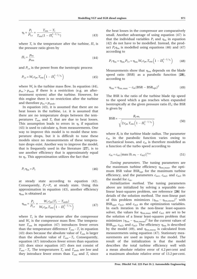
using few parameters [29]. The submodel (53) is

compared with calculated points from measure-

ments in Fig. 5(a) where the points are calculated

by solving equation (52) for fPt. Note that this com-

parison is not a validation of the submodel since

the calculated points depend on the model tuning.

When the VGT control signal uvgt increases, the

effective area increases and hence also the flow

increases. Because of the geometry of the turbine,

the change in the effective area is large when the

VGT control signal is small. This behaviour can be

described by a part of an ellipse

fvgt(~uvgt)� cf2

cf1

2

+~uvgt � cvgt2

cvgt1

2

= 1 (54)

0.2 0.3 0.4 0.5 0.6 0.7 0.8 0.9 1

0.6

0.8

1

1.(a)

(b)

2

f Πt [−

]

Πt[−]

20 30 40 50 60 70 80 90 100 1100.4

0.6

0.8

1

1.2

1.4

f vgt[−

]

uvgt

[%]

Fig. 5 Comparison of calculated points from measurements and the two submodels given in (a)equation (53) and (b) equation (56) in the turbine mass flow model at steady state showinghow different variables in the submodels depend on each other



where fvgt is the effective area ratio function and~uvgt describes the VGT actuator dynamics.

The flow can now be modelled by solving equa-

tion (52) for Wt giving

Wt =Avgtmax pem fPt(Pt) fvgt(~uvgt)ffiffiffiffiffiffiffiffiffiffiffiffiffiffi

Tem Re

p (55)

and solving equation (54) for fvgt, giving

fvgt(~uvgt) = cf2 + cf1

ffiffiffiffiffiffiffiffiffiffiffiffiffiffiffiffiffiffiffiffiffiffiffiffiffiffiffiffiffiffiffiffiffiffiffiffiffiffiffiffiffiffiffiffiffiffiffiffiffiffiffiffiffiffiffiffiffiffiffimax (0, 1�

~uvgt � cvgt2

cvgt1

� �2

)

s(56)

The submodel (56) is compared with calculated

points from measurements in Fig. 5(b) where the

points are calculated by solving equation (52) for

fvgt. Note that this comparison is not a validation of

the submodel since the calculated points depend

on the model tuning.Tuning parameters. The tuning parameters are

the exponent Kt in the choking function for the tur-

bine flow and the parameters cf1, cf2, cvgf1, and cvgf2

in the ellipse for the effective area ratio function.Initialization method. The tuning parameters

above are initialized by solving a non-linear least-

squares problem that minimizes (Wt – Wt,meas)2

with the tuning parameters as the optimization

variables. The flow Wt is described by the model

(55), (56), and (53), and Wt,meas is calculated from

measurements as Wt,meas = Wc + Wf, where Wf is

calculated using equation (13). Stationary mea-

surements are used as inputs to the model. The

result of the initialization is that the turbine mass

flow model has small absolute relative errors with

a mean absolute relative error of 2.8 per cent and

a maximum absolute relative error of 7.6 per cent.

The parameters are then tuned according to the


6.2.3 VGT actuator

The VGT actuator dynamics are modelled as a first-

order system with a time delay according to

d

dt~uvgt =

1

tvgt(uvgt(t � tdvgt)� ~uvgt) (57)


the time constant tvgt and the time delay tdvgt.Tuning method. The tuning parameters above are

determined by solving a non-linear least-squares

problem that minimizes ( ~uvgt – ~uvgt,meas)2 with tvgt

and tdvgt as the optimization variables. The vari-

able ~uvgt is the model in equation (57) and ~uvgt,meas

are dynamic responses in the dynamic data set J in

Table 1. These data consist of 18 steps in the VGT

position with a step size of 10 per cent, going from

100 per cent down to 10 per cent and then back

again to 100 per cent with a step size of 10 per cent.

The measurements also consist of five steps with

a step size of 5 per cent and one step with a step size

of 20 per cent. These 24 steps are then normalized

and shifted in time in order to achieve the

same starting point. These measurements are then

compared with the unit step response for the

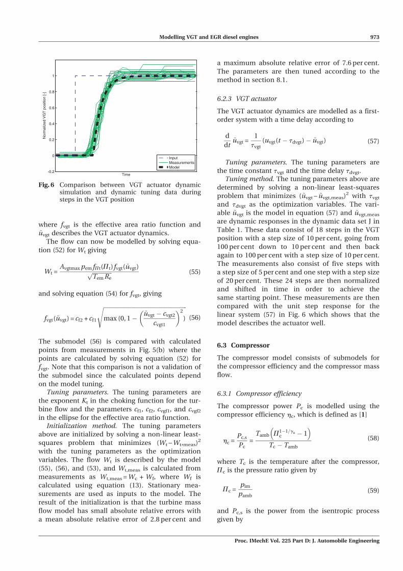
linear system (57) in Fig. 6 which shows that the

model describes the actuator well.

6.3 Compressor

The compressor model consists of submodels for

the compressor efficiency and the compressor mass

flow.

6.3.1 Compressor efficiency

The compressor power Pc is modelled using the

compressor efficiency hc, which is defined as [1]

hc =Pc,s

Pc=

Tamb P1�1=gac � 1

� �Tc � Tamb

(58)

where Tc is the temperature after the compressor,

Pc is the pressure ratio given by

Pc =pim

pamb(59)

and Pc,s is the power from the isentropic process

given by

-0.2

0

0.2

0.4

0.6

0.8

1

Nor

mal

ized

VG

T p

ositi

on [-

]

Time

InputMeasurementsModel

Fig. 6 Comparison between VGT actuator dynamicsimulation and dynamic tuning data duringsteps in the VGT position



Pc,s = Wc cpa Tamb P1�1=gac � 1

� �(60)

where Wc is the compressor mass flow. The power

Pc is modelled by solving equation (58) for Pc and

using equation (60) according to

Pc =Pc,s

hc

=Wc cpa Tamb

hc

P1�1=gac � 1

� �(61)

The efficiency is modelled using ellipses similar

to the method in reference [30], but with a non-

linear transformation on the axis for the pressure

ratio similar to the method in reference [25]. The

inputs to the efficiency model are Pc and Wc (see

Fig. 7). The flow Wc is not scaled by the inlet tem-

perature and the inlet pressure, in the current

implementation, since these two variables are con-

stant. However, this model can easily be extended

with a corrected mass flow in order to consider var-

iations in the environmental conditions.

The ellipses can be described as

hc = hcmax � xT Qc x (62)

x is a vector which contains the inputs according to

x =Wc �Wcopt

pc � pcopt

(63)

where the non-linear transformation for Pc is

pc = Pc � 1ð Þcp (64)

and the symmetric and positive semidefinite matrix

Qc consists of three parameters according to

Qc =a1 a3

a3 a2

(65)

Tuning model parameters. The tuning model

parameters are the maximum compressor efficiency

hcmax, the optimum value Wcopt of Wc and the opti-

mum value pcopt of pc for the maximum compres-

sor efficiency, the exponent cp in the scale function

(64), and the parameters a1, a2, a3 in the matrix Qc.Initialization method. The tuning parameters




of this problem minimizes (hc – hc,meas)2 with Wcopt,

pcopt, and cp as the optimization variables. In each

0 0.1 0.2 0.3 0.4 0.5 0.6 0.71

1.5

2

2.5

3

3.5

4

Wc [kg/s]

Πc [−

]

0.5

0.5

0.5

0.5

0.5

0.5

0.55

0.55

0.55

0.55

0.55

0.55

0.6

0.6

0.6

0.6

0.6

0.6

0.60.

65

0.65

0.65

0.65

0.65

0.65

0.65

0.7

0.7

0.7

0.7

0.7

0.7

0.7

0.73

0.73

0.73

0.73

40005000

6000

7000

8000

9000

10000

11000

12000

ηc < 0.5

0.5 < ηc < 0.55

0.55 < ηc < 0.6

0.6 < ηc < 0.65

0.65 < ηc < 0.7

0.7 < ηc < 0.73

0.73 < ηc

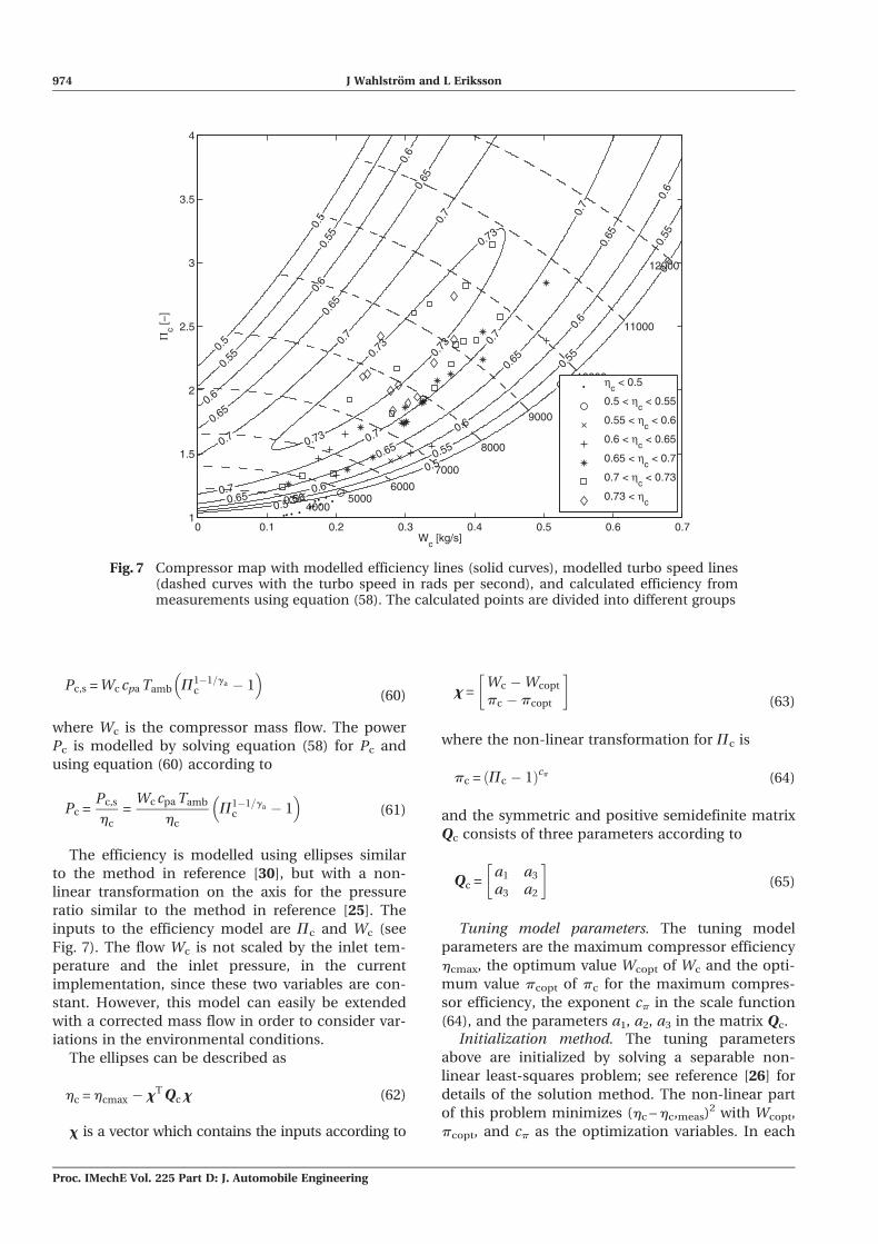
Fig. 7 Compressor map with modelled efficiency lines (solid curves), modelled turbo speed lines(dashed curves with the turbo speed in rads per second), and calculated efficiency frommeasurements using equation (58). The calculated points are divided into different groups



iteration in the non-linear least-squares solver, the

values for hcmax, a1, a2, and a3 are set to be the

solution of a linear least-squares problem that

minimizes (hc – hc,meas)2 for the current values of

Wcopt, pcopt, and cp. The efficiency hc is described

by the models (62) to (65) and hc,meas is calculated

from measurements using equation (58).

Stationary measurements are used as inputs to the

model. The result of the initialization is that the

compressor efficiency model has small absolute

relative errors with a mean absolute relative error

of 3.3 per cent and a maximum absolute relative

error of 14.1 per cent. The parameters are then

tuned according to the method in section 8.1,

which guarantees that the matrix Qc becomes posi-

tive semidefinite using the expression in the

compressor efficiency model during the tuning

given by

a3 := min½max (a3, �ffiffiffiffiffiffiffiffiffiffia1 a2

p),

ffiffiffiffiffiffiffiffiffiffia1 a2

p�

6.3.2 Compressor mass flow

The mass flow Wc through the compressor is mod-

elled using two dimensionless variables. The first

variable is the energy transfer coefficient [31]

Cc =2cpa Tamb P1�1=ga

c � 1� �R2

c v2t

(66)

which is the ratio of the isentropic kinetic energy of

the gas at the given pressure ratio Pc to the kinetic

energy of the compressor blade tip where Rc is the

compressor blade radius. The second variable is the

volumetric flow coefficient [31]

Fc =Wc=ramb

pR3c vt

=Ra Tamb

pamb p R3c vt

Wc (67)

which is the ratio of the volume flowrate of air into

the compressor to the rate at which volume is

displaced by the compressor blade where ramb is

the density of the ambient air. The relation between

Cc and Fc can be described by a part of an ellipse

[25, 27]

cC1(vt) Cc � cC2ð Þ2 + cF1(vt) Fc � cF2ð Þ2 = 1 (68)

where cC1 and cF1 vary with the turbo speed vt and

are modelled as the polynomial functions

cC1(vt) = cvC1 v2t + cvC2 vt + cvC3 (69)

cF1(vt) = cvF1 v2t + cvF2 vt + cvF3 (70)

The mass flow is modelled by solving equa-

tion (68) for Fc and solving equation (67) for Wc

according to

Fc =

ffiffiffiffiffiffiffiffiffiffiffiffiffiffiffiffiffiffiffiffiffiffiffiffiffiffiffiffiffiffiffiffiffiffiffiffiffiffiffiffiffiffiffiffiffiffiffiffiffiffiffiffiffiffiffiffiffiffiffiffiffiffiffimax 0,

1� cC1 Cc � cC2ð Þ2

cF1

!vuut + cF2(71)

Wc =pamb pR3

c vt

Ra TambFc (72)

Tuning model parameters. The tuning parameters

are the parameters cC2 and cF2 in the ellipse model

for the compressor mass flow, the coefficients cvC1,

cvC2 and cvC3 in the polynomial function (69) and

the coefficients cvF1, cvF2 and cvF3 in the polyno-

mial function (70).Initialization method. The tuning parameters




of this problem minimizes (cC1(vt)(Cc–cC2)2 +

cF1(vt)(Fc–cF2)2–1)2 with cC2 and cF2 as the optimi-

zation variables. In each iteration in the non-linear

least-squares solver, the values for cvC1, cvC2, cvC3,

cvF1, cvF2, and cvF3 are set to be the solution of

a linear least-squares problem that minimizes

(cC1(vt)(Cc – cC2)2 + cF1(vt)(Fc – cF2)2–1)2 for the cur-

rent values of cC2 and cF2. Stationary measurements

are used as inputs to the model. The result of the

initialization is that the model describes the com-

pressor mass flow well with a mean absolute rela-

tive error of 3.4 per cent and a maximum absolute

relative error of 13.7 per cent. The parameters are

then tuned according to the method in section 8.1.

6.3.3 Compressor map

The compressor performance is usually presented

in terms of a map with Pc and Wc on the axes

showing the curves of constant efficiency and con-

stant turbo speed. This is shown in Fig. 7 which has

approximately the same characteristics as Fig. 2.10

in reference [28]. Consequently, the proposed

model of the compressor efficiency equation (62)

and the compressor flow equation (72) has the

expected behaviour.

7 INTERCOOLER AND EGR COOLER

To construct a simple model, that captures the

important system properties, the intercooler and

the EGR cooler are assumed to be ideal, i.e. there is



no pressure loss, no mass accumulation, and per-

fect efficiency, which gives the equations

pout = pin, Wout = Win, Tout = Tcool (73)

where Tcool is the cooling temperature. The model

can be extended with non-ideal coolers, but these

increase the complexity of the model since non-

ideal coolers require that there are states for the

pressures both before and after the coolers.

8 MODEL TUNING AND VALIDATION

One step in the development of a model that

describes the system dynamics and the non-linear

effects is the tuning and validation. In section 8.1 the

model tuning is described, in section 8.2 the impor-

tance of different steps in the tuning method is illus-

trated, and in section 8.3 a validation of the complete

model is performed using dynamic data. In the vali-

dation, it is important to investigate whether the

model captures the essential dynamic behaviours

and non-linear effects. The data that are used in the

tuning and validation are described in section 2.2.

8.1 Tuning

As described in section 2.3, the model parameters

are estimated in five steps.

8.1.1 Initialization method

First, the parameters in the static models are initial-

ized automatically using least-squares optimization

and tuning data from stationary measurements. The

initialization methods for each parameter and the

results are described in sections 4 to 6.

8.1.2 Parameters in dynamic models

Second, the actuator parameters are estimated using

the method in sections 5.2 and 6.2.3. These sections

also show the tuning results for the actuators.

Third, the manifold volumes and the turbo-

charger inertia are estimated by solving the least-

squares optimization problem

min V (u)

s:t: umin � u � umax (74)

where V(u) is the cost function given by

V (u)=XK

k =1

XJ

j =1

1

Lj

XLj

l =1

wmeas,dynk ½l��w

mod,dynk ½l�

� �2

(75)

and u represents the manifold volumes and the

turbocharger inertia, and umin and umax are the lower

bound and the upper bound respectively for the

parameters. The cost function minimizes the errors

between the dynamic measurements wmeas,dynk and

the dynamic simulations wmod,dynk of the complete

model. There are four outputs (K = 4) in the dynamic

measurements and simulations, as given by

w1 = pnormim , w2 = pnorm

em , w3 = W normc , w4 = nnorm

t

where each output and each step response is normal-

ized so that the initial and final values for each step

response are the same for both the measurements

and the simulations, i.e. there are only dynamic

errors in the outputs and no stationary errors.

Further, J is the number of data sets in the

dynamic measurements with J = 2 where the data

sets are the sets B and C in Table 1. The constant Lj

is the number of samples in data set j where both

dynamic measurements and simulations are sam-

pled with a frequency of 100 Hz. The sumPLj

l = 1 of

each data set in the cost function is normalized

with Lj in order to penalize each data set equally.

Fourth, the time constant for the engine torque is

estimated in the following way. A dynamometer is

fitted to the engine via an axle shaft in order to

brake or supply torque to the engine. This dyna-

mometer and axle shaft lead to the fact that the

measured engine torque has a time constant (see

Fig. 19 on page 61 of reference [9]) which is not

modelled because the torque will not be used as

a feedback in the controller. However, in order to

validate the engine torque model during dynamic

responses, these dynamics are modelled in the

validation as a first-order system

d

dtMdynamo =

1

tM e

(Me �Mdynamo) (76)

where Mdynamo is the torque in the dynamometer

and Me is the output torque from the engine. The

time constant tMeis tuned by solving the same opti-

mization problem as in equations (74) and (75) but

with u = tMe, K = 1, and J = 1 with the data set I in

Table 1, w1 = Mnormdynamo, and where both dynamic

measurements and simulations are sampled with

a frequency of 10 Hz.

8.1.3 Parameters in the static models

Fifth, the parameters in static models are finally

estimated automatically using a least-squares opti-

mization that minimizes errors both in the submo-

dels and in the complete model. This optimization

problem is formulated in the same way as in equa-

tion (74) but with the cost function



V (u) =1

KJ

XK

k = 1

XJ

j = 1

g2j

Lj

XLj

l = 1

ymeas,dynk ½l� � y

mod,dynk ½l�

1M

PMm = 1

ymeas,statk ½m�

0BBB@

1CCCA

2

+1

bNM

XN

n = 1

XMp = 1

zmeas,statn ½p� � zmod,stat

n ½p�1

M

PMm = 1

zmeas,statn ½m�

0BBB@

1CCCA

2

(77)

where u represents the static model parameters.

The first row in the cost function minimizes the

errors between dynamic measurements ymeas,dynk

and dynamic simulations ymod,dynk of the complete

model. The second row minimizes the errors

between stationary measurements zmeas,statn and

static submodels zmod,statn . There are four outputs

(K = 4) in the dynamic measurements and simula-

tions, namely

y1 = pim, y2 = pem, y3 = Wc, y4 = nt

and there are seven outputs (N = 7) in the stationary

measurements and static submodels, namely

z1 = Wei, z2 = Tem, z3 = Wegr, z4 = htm,

z5 = Wt, z6 = hc, z7 = Wc

The signals zmeas,statn and zmod,stat

n are calculated

according to the initialization methods in sections 4

to 6. Further, the number J of data sets in the

dynamic measurements is 9 where the data sets are

the sets A to I in Table 1. Both the dynamic mea-

surements and the simulations are sampled at a fre-

quency of 10 Hz. The constant M is the number of

operating points in the stationary measurements

with M = 82.

Each term in the first row in the cost function is

normalized with the mean value of the stationary

measurements for the outputs ymeas,statk and each

term in the second row is normalized with the

mean value of the stationary measurements for the

outputs zmeas,statn . Further, the first row is normalized

with KJ and the second row is normalized with NM

in order penalize dynamic and stationary measure-

ments equally. The parameters b and gj are tuning

parameters in the optimization problem and they

are set to

b = 1, g7 = 2, g8 = 4, gj = 1, for j = 1, . . . , 6, 9

The optimization problem is solved using a stan-

dard MATLAB local non-linear least-squares solver

and the parameters are initialized using the method

in the first step above. The result of the optimiza-

tion is given in Table 2, showing that the mean

absolute relative errors are 4.8 per cent or lower.

The calculation time for evaluating the cost func-

tion (77) is 42 s in MATLAB/Simulink on a personal

computer with an Intel Core 2 Quad (2.8 GHz), and

this cost function was evaluated 190 times when the

optimization problem (74) and (77) was solved.

Further, the calculation time for simulating the

model on the European transient cycle is 28 s,

where the cycle is 1800 s long.

To investigate how much the tuning affects the

values of the intake manifold volume Vim and the

exhaust manifold volume Vem, the physical values

of these two parameters are compared with the

optimization results. The physical value of Vim is

37 dm3 (which also includes the intercooler volume

since they are lumped in the model) and the opti-

mization result is 45 dm3, i.e. an increase of 22 per

cent. The physical value of Vem is 20 dm3 and the

optimization result is 23 dm3, i.e. an increase of

15 per cent. These deviations are reasonable in com-

bination with the fact that they are both increased.

The increase can also to some extent be attributed

to the additional volumes of fitting pipes as well as

the inlets and outlet of neighbouring components

which are not included in the values of the physical

components volume but these do contribute to the

dynamic response in the lumped-parameter model.

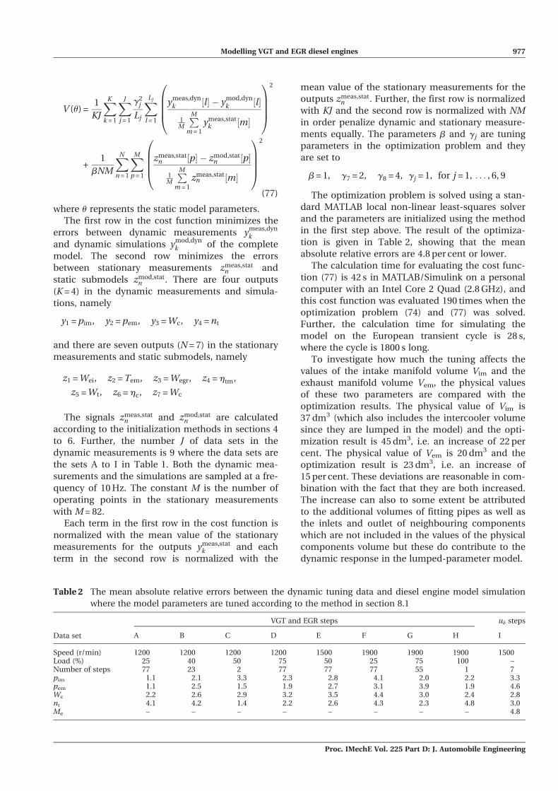
Table 2 The mean absolute relative errors between the dynamic tuning data and diesel engine model simulation

where the model parameters are tuned according to the method in section 8.1

Data set

VGT and EGR steps ud steps

A B C D E F G H I

Speed (r/min) 1200 1200 1200 1200 1500 1900 1900 1900 1500Load (%) 25 40 50 75 50 25 75 100 –Number of steps 77 23 2 77 77 77 55 1 7pim 1.1 2.1 3.3 2.3 2.8 4.1 2.0 2.2 3.3pem 1.1 2.5 1.5 1.9 2.7 3.1 3.9 1.9 4.6Wc 2.2 2.6 2.9 3.2 3.5 4.4 3.0 2.4 2.8nt 4.1 4.2 1.4 2.2 2.6 4.3 2.3 4.8 3.0Me – – – – – – – – 4.8



The fuel injection ud was not measured in the

data sets A to H. In order to obtain values for ud for

these measurements, ud is calculated by inverting

the engine torque model (26) to (31), (76) with ud as

the input and Mdynamo as the output. This means

that there will be no errors for the engine torque

model. Therefore Me is not included in the outputs

yk and zn, the engine torque model parameters are

not included in u, and the errors for the engine

torque are not calculated for the data sets A to H in

Table 2. This will not affect the tuning of the other

model parameters since the engine torque does not

affect the outputs yk and zn.

8.2 The importance of the initialization methodand the cost function (77)

To illustrate the importance of the initialization

method in the first step in the proposed tuning

method and the cost function (77), the tuning method

in section 8.1 is compared with two other tuning

methods.

First, if each parameter u(i) in the static models

is initialized to

u(i) =umax(i) if umax(i)\1

1 if umin(i) � 1 � umax(i)umin(i) if umin(i).1

8<: (78)

and if only the first row is used in equation (77), i.e.

the complete model (which is a common choice of

cost function in system identification), the mean

absolute relative errors become 480 per cent or

lower when a local solver is applied. This high error

arises because the optimization is non-convex with

at least two local minima. Consequently, by opti-

mizing the sub-models in the initialization a simple

local solver can be used for the non-convex opti-

mization problem to obtain small errors in the

complete model. It is also important to use the

submodels in the cost function to guarantee that

each submodel describes the measurements well.

Second, if only the first four steps in the tuning

method are used (which is a common choice of

tuning method for mean value engine models), the

mean absolute relative errors become 12.7 per cent

or lower, compared with 4.8 per cent or lower for

the proposed tuning method. Consequently, it is

important to use both the submodels and the com-

plete model in the optimization and not only the

submodels.

8.3 Validation

Because there are few stationary measurements,

both the static and the dynamic models are vali-

dated by simulating the total model and comparing

it with the dynamic validation data sets Q to V in

Table 1. The result of this validation can be seen in

Table 3 which shows that the mean absolute rela-

tive errors are 5.8 per cent or lower. The relative

errors are due mostly to steady state errors but,

since the engine model will be used in a controller,

the steady state accuracy is less important since

a controller will take care of steady state errors.

However, in order to design a successful controller,

it is important that the model captures the main

steady state behaviours, essential dynamic beha-

viours, and non-linear effects. Therefore, essential

system properties and time constants are validated

in the following section.

8.3.1 Validation of essential system properties andtime constants

References [2] and [3] show the essential system

properties for the pressures and the flows in

a diesel engine with VGT and EGR. Some of these

properties are a non-minimum phase behaviour in

the intake manifold pressure and a non-minimum

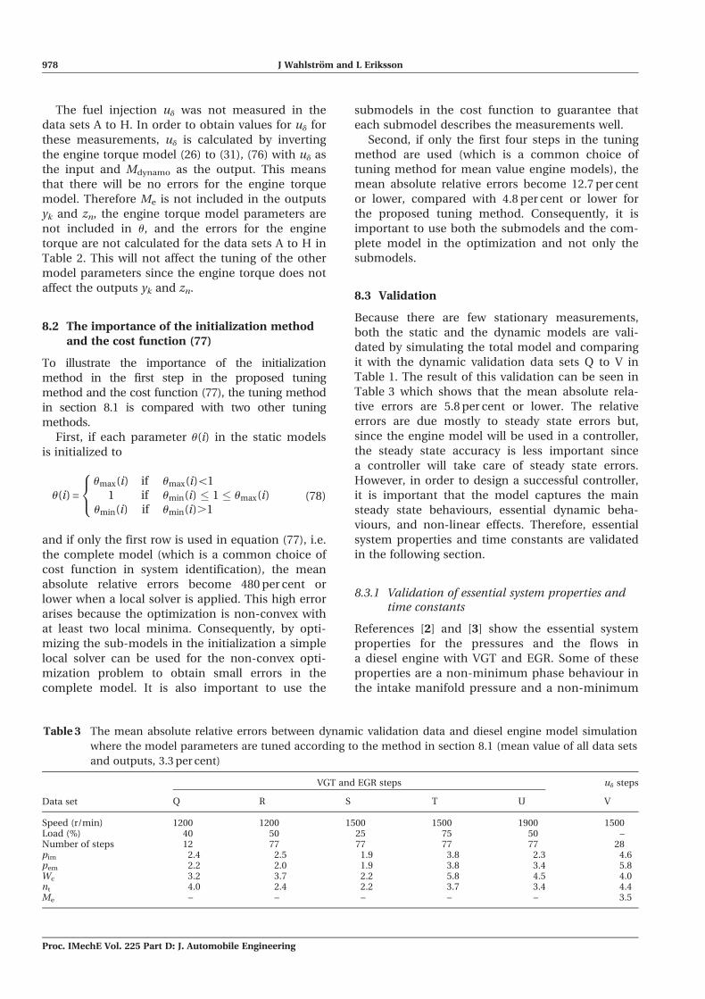
Table 3 The mean absolute relative errors between dynamic validation data and diesel engine model simulation

where the model parameters are tuned according to the method in section 8.1 (mean value of all data sets

and outputs, 3.3 per cent)

Data set


Q R S T U V

Speed (r/min) 1200 1200 1500 1500 1900 1500Load (%) 40 50 25 75 50 –Number of steps 12 77 77 77 77 28pim 2.4 2.5 1.9 3.8 2.3 4.6pem 2.2 2.0 1.9 3.8 3.4 5.8Wc 3.2 3.7 2.2 5.8 4.5 4.0nt 4.0 2.4 2.2 3.7 3.4 4.4Me – – – – – 3.5



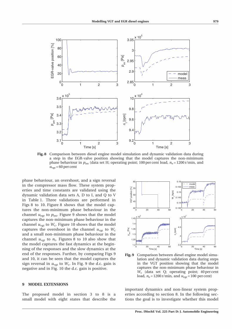
phase behaviour, an overshoot, and a sign reversal

in the compressor mass flow. These system prop-

erties and time constants are validated using the

dynamic validation data sets A, D to I, and Q to V

in Table 1. Three validations are performed in

Figs 8 to 10. Figure 8 shows that the model cap-

tures the non-minimum phase behaviour in the

channel uegr to pim. Figure 9 shows that the model

captures the non-minimum phase behaviour in the

channel uvgt to Wc. Figure 10 shows that the model

captures the overshoot in the channel uvgt to Wc

and a small non-minimum phase behaviour in the

channel uvgt to nt. Figures 8 to 10 also show that

the model captures the fast dynamics at the begin-

ning of the responses and the slow dynamics at the

end of the responses. Further, by comparing Figs 9

and 10, it can be seen that the model captures the

sign reversal in uvgt to Wc. In Fig. 9 the d.c. gain is

negative and in Fig. 10 the d.c. gain is positive.

9 MODEL EXTENSIONS

The proposed model in section 3 to 8 is a

small model with eight states that describe the

important dynamics and non-linear system prop-

erties according to section 8. In the following sec-

tions the goal is to investigate whether this model

0 1 2 30

20

40

60

80

100

EG

R-v

alve

pos

ition

[%]

0 1 2 32.85

2.9

2.95

3

3.05x 10

5

p im [P

a]

modelmeas

0 1 2 33.1

3.2

3.3

3.4

3.5

3.6x 10

5

p em [P

a]

Time [s]0 1 2 3

9.2

9.4

9.6

9.8

10x 10

4

n t [rpm

]

Time [s]

Fig. 8 Comparison between diesel engine model simulation and dynamic validation data duringa step in the EGR-valve position showing that the model captures the non-minimumphase behaviour in pim (data set H; operating point; 100 per cent load, ne = 1200 r/min, anduvgt = 60 per cent

0 20 40 6040

45

50

55

60

VG

T p

ositi

on [%

]

0 20 40 600.135

0.14

0.145

0.15

0.155

0.16

Wc [k

g/s]

modelmeas

0 20 40 601.2

1.25

1.3

1.35

1.4

1.45x 10

5

p em [P

a]

Time [s]0 20 40 60

3.5

4

4.5

5x 10

4

n t [rpm

]

Time [s]

Fig. 9 Comparison between diesel engine model simu-lation and dynamic validation data during stepsin the VGT position showing that the modelcaptures the non-minimum phase behaviour inWc (data set Q; operating point; 40 per centload, ne = 1200 r/min, and uegr = 100 per cent)



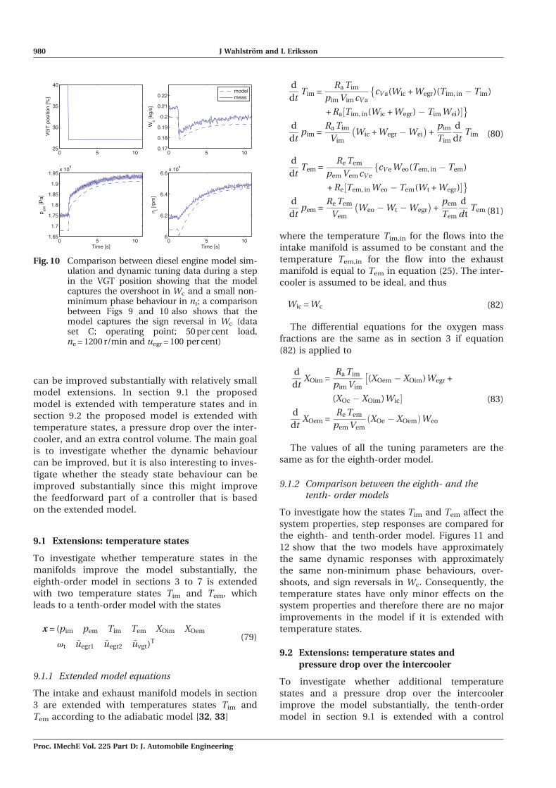
can be improved substantially with relatively small

model extensions. In section 9.1 the proposed

model is extended with temperature states and in

section 9.2 the proposed model is extended with

temperature states, a pressure drop over the inter-

cooler, and an extra control volume. The main goal

is to investigate whether the dynamic behaviour

can be improved, but it is also interesting to inves-

tigate whether the steady state behaviour can be

improved substantially since this might improve

the feedforward part of a controller that is based

on the extended model.

9.1 Extensions: temperature states

To investigate whether temperature states in the

manifolds improve the model substantially, the

eighth-order model in sections 3 to 7 is extended

with two temperature states Tim and Tem, which

leads to a tenth-order model with the states

x = (pim pem Tim Tem XOim XOem

vt ~uegr1 ~uegr2 ~uvgt)T (79)

9.1.1 Extended model equations

The intake and exhaust manifold models in section

3 are extended with temperatures states Tim and

Tem according to the adiabatic model [32, 33]

d

dtTim =

Ra Tim

pim Vim cV acV a(Wic + Wegr)(Tim, in � Tim)�

+ Ra½Tim, in(Wic + Wegr)� Tim Wei)��

d

dtpim =

Ra Tim

VimWic + Wegr �Wei

� �+

pim

Tim

d

dtTim (80)

d

dtTem =

Re Tem

pem Vem cV ecV e Weo(Tem, in � Tem)f

+ Re½Tem, in Weo � Tem(Wt + Wegr)��

d

dtpem =

Re Tem

VemWeo �Wt �Wegr

� �+

pem

Tem

d

dtTem (81)

where the temperature Tim,in for the flows into the

intake manifold is assumed to be constant and the

temperature Tem,in for the flow into the exhaust

manifold is equal to Tem in equation (25). The inter-

cooler is assumed to be ideal, and thus

Wic = Wc (82)

The differential equations for the oxygen mass

fractions are the same as in section 3 if equation

(82) is applied to

d

dtXOim =

Ra Tim

pim Vim(XOem � XOim)Wegr +

(XOc � XOim)Wic�d

dtXOem =

Re Tem

pem VemXOe � XOemð ÞWeo

(83)

The values of all the tuning parameters are the

same as for the eighth-order model.

9.1.2 Comparison between the eighth- and thetenth- order models

To investigate how the states Tim and Tem affect the

system properties, step responses are compared for

the eighth- and tenth-order model. Figures 11 and

12 show that the two models have approximately

the same dynamic responses with approximately

the same non-minimum phase behaviours, over-

shoots, and sign reversals in Wc. Consequently, the

temperature states have only minor effects on the

system properties and therefore there are no major

improvements in the model if it is extended with

temperature states.

9.2 Extensions: temperature states and

pressure drop over the intercooler

To investigate whether additional temperature

states and a pressure drop over the intercooler

improve the model substantially, the tenth-order

model in section 9.1 is extended with a control

0 5 1025

30

35

40

VG

T p

ositi

on [%

]

0 5 100.17

0.18

0.19

0.2

0.21

0.22

Wc [k

g/s]

modelmeas

0 5 101.65

1.7

1.75

1.8

1.85

1.9

1.95x 10

5

p em [P

a]

Time [s]0 5 10

6

6.2

6.4

6.6x 10

4

n t [rpm

]

Time [s]

Fig. 10 Comparison between diesel engine model sim-ulation and dynamic tuning data during a stepin the VGT position showing that the modelcaptures the overshoot in Wc and a small non-minimum phase behaviour in nt; a comparisonbetween Figs 9 and 10 also shows that themodel captures the sign reversal in Wc (dataset C; operating point; 50 per cent load,ne = 1200 r/min and uegr = 100 per cent)



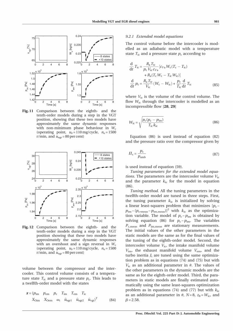
volume between the compressor and the inter-

cooler. This control volume consists of a tempera-

ture state Tic and a pressure state pc. This leads to

a twelfth-order model with the states

x = (pim pem pc Tim Tem Tic

XOim XOem vt ~uegr1 ~uegr2 ~uvgt)T

(84)

9.2.1 Extended model equations

The control volume before the intercooler is mod-

elled as an adiabatic model with a temperature

state Tic and a pressure state pc according to

d

dtTic =

Ra Tic

pc Vic cV acV a Wc(Tc � Tic)½

+ Ra(Tc Wc � Tic Wic)�d

dtpc =

Ra Tic

VicWc �Wicð Þ+

pc

Tic

d

dtTic (85)

where Vic is the volume of the control volume. The

flow Wic through the intercooler is modelled as an

incompressible flow [28, 29]

Wic =

ffiffiffiffiffiffiffiffiffiffiffiffiffiffiffiffiffiffiffiffiffiffiffiffiffiffipc(pc � pim)

Tic kic

s(86)

Equation (86) is used instead of equation (82)

and the pressure ratio over the compressor given by

Pc =pc

pamb(87)

is used instead of equation (59).Tuning parameters for the extended model equa-

tions. The parameters are the intercooler volume Vic

and the parameter kic for the model in equation

(86).Tuning method. All the tuning parameters in the

twelfth-order model are tuned in three steps. First,

the tuning parameter kic is initialized by solving

a linear least-squares problem that minimizes [pc –

pim – (pc,meas – pim,meas)]2 with kic as the optimiza-

tion variable. The model of pc – pim is obtained by

solving equation (86) for pc – pim. The variables

Pc,meas and Pim,meas are stationary measurements.

The initial values of the other parameters in the

static models are the same as for the final values of

the tuning of the eighth-order model. Second, the

intercooler volume Vic, the intake manifold volume

Vim, the exhaust manifold volume Vem, and the

turbo inertia Jt are tuned using the same optimiza-

tion problem as in equations (74) and (75) but with

Vic as an additional parameter in u. The values of

the other parameters in the dynamic models are the

same as for the eighth-order model. Third, the para-

meters in static models are finally estimated auto-

matically using the same least-squares optimization

problem as in equations (74) and (77) but with kic

as an additional parameter in u, N = 8, z8 = Wic, and

b = 2.58.

0 2 4 6 8

65

70

75

u vgt [%

]

0 2 4 6 80.225

0.23

0.235

0.24

Wc [k

g/s]

8 states10 states

0 2 4 6 81.42

1.44

1.46

1.48

1.5

1.52x 10

5

p im [P

a]

Time [s]0 2 4 6 8

1.5

1.55

1.6x 10

5p em

[Pa]

Time [s]

Fig. 11 Comparison between the eighth- and thetenth-order models during a step in the VGTposition, showing that these two models haveapproximately the same dynamic responseswith non-minimum phase behaviour in Wc

(operating point, ud = 110 mg/cycle, ne = 1500r/min, and uegr = 80 per cent)

0 2 4 6 824

26

28

30

u vgt [%

]

0 2 4 6 80.23

0.235

0.24

0.245

Wc [k

g/s]

8 states10 states

0 2 4 6 8

1.94

1.96

1.98

x 105

p im [P

a]

Time [s]0 2 4 6 8

2.15

2.2

2.25

2.3

2.35x 10

5

p em [P

a]

Time [s]

Fig. 12 Comparison between the eighth- and thetenth-order models during a step in the VGTposition showing that these two models haveapproximately the same dynamic responseswith an overshoot and a sign reversal in Wc

(operating point, ud = 110 mg/cycle, ne = 1500r/min, and uegr = 80 per cent)



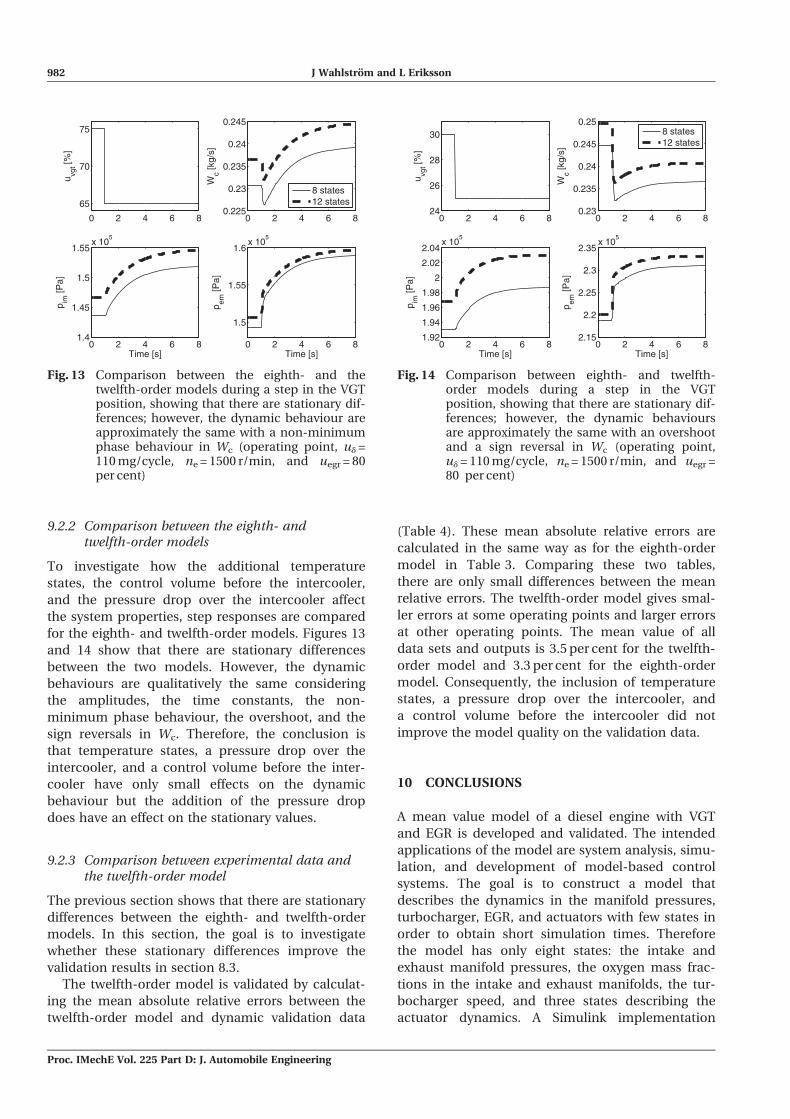
9.2.2 Comparison between the eighth- andtwelfth-order models

To investigate how the additional temperature

states, the control volume before the intercooler,

and the pressure drop over the intercooler affect

the system properties, step responses are compared

for the eighth- and twelfth-order models. Figures 13

and 14 show that there are stationary differences

between the two models. However, the dynamic

behaviours are qualitatively the same considering

the amplitudes, the time constants, the non-

minimum phase behaviour, the overshoot, and the

sign reversals in Wc. Therefore, the conclusion is

that temperature states, a pressure drop over the

intercooler, and a control volume before the inter-

cooler have only small effects on the dynamic

behaviour but the addition of the pressure drop

does have an effect on the stationary values.

9.2.3 Comparison between experimental data andthe twelfth-order model

The previous section shows that there are stationary

differences between the eighth- and twelfth-order

models. In this section, the goal is to investigate

whether these stationary differences improve the

validation results in section 8.3.

The twelfth-order model is validated by calculat-

ing the mean absolute relative errors between the

twelfth-order model and dynamic validation data

(Table 4). These mean absolute relative errors are

calculated in the same way as for the eighth-order

model in Table 3. Comparing these two tables,

there are only small differences between the mean

relative errors. The twelfth-order model gives smal-

ler errors at some operating points and larger errors

at other operating points. The mean value of all

data sets and outputs is 3.5 per cent for the twelfth-

order model and 3.3 per cent for the eighth-order

model. Consequently, the inclusion of temperature

states, a pressure drop over the intercooler, and

a control volume before the intercooler did not

improve the model quality on the validation data.

10 CONCLUSIONS

A mean value model of a diesel engine with VGT

and EGR is developed and validated. The intended

applications of the model are system analysis, simu-

lation, and development of model-based control

systems. The goal is to construct a model that

describes the dynamics in the manifold pressures,

turbocharger, EGR, and actuators with few states in

order to obtain short simulation times. Therefore

the model has only eight states: the intake and

exhaust manifold pressures, the oxygen mass frac-

tions in the intake and exhaust manifolds, the tur-

bocharger speed, and three states describing the

actuator dynamics. A Simulink implementation

0 2 4 6 8

65

70

75

u vgt [%

]

0 2 4 6 80.225

0.23

0.235

0.24

0.245

Wc [k

g/s]

8 states12 states

0 2 4 6 81.4

1.45

1.5

1.55x 10

5

p im [P

a]

Time [s]0 2 4 6 8

1.5

1.55

1.6x 10

5

p em [P

a]

Time [s]

Fig. 13 Comparison between the eighth- and thetwelfth-order models during a step in the VGTposition, showing that there are stationary dif-ferences; however, the dynamic behaviour areapproximately the same with a non-minimumphase behaviour in Wc (operating point, ud =110 mg/cycle, ne = 1500 r/min, and uegr = 80per cent)

0 2 4 6 824

26

28

30

u vgt [%

]

0 2 4 6 80.23

0.235

0.24

0.245

0.25

Wc [k

g/s]

8 states12 states

0 2 4 6 81.92

1.94

1.96

1.98

2

2.02

2.04x 10

5

p im [P

a]

Time [s]0 2 4 6 8

2.15

2.2

2.25

2.3

2.35x 10

5

p em [P

a]

Time [s]

Fig. 14 Comparison between eighth- and twelfth-order models during a step in the VGTposition, showing that there are stationary dif-ferences; however, the dynamic behavioursare approximately the same with an overshootand a sign reversal in Wc (operating point,ud = 110 mg/cycle, ne = 1500 r/min, and uegr =80 per cent)



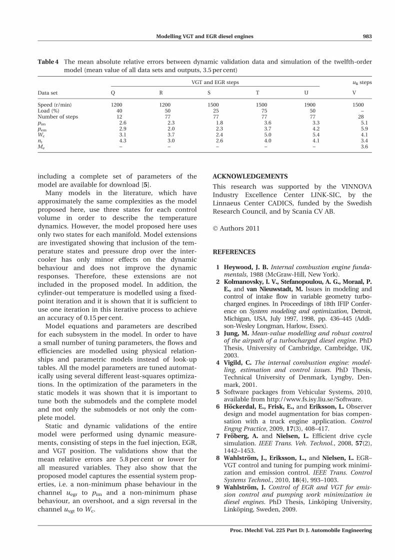
including a complete set of parameters of the

model are available for download [5].

Many models in the literature, which have

approximately the same complexities as the model

proposed here, use three states for each control

volume in order to describe the temperature

dynamics. However, the model proposed here uses

only two states for each manifold. Model extensions

are investigated showing that inclusion of the tem-

perature states and pressure drop over the inter-

cooler has only minor effects on the dynamic

behaviour and does not improve the dynamic

responses. Therefore, these extensions are not

included in the proposed model. In addition, the

cylinder-out temperature is modelled using a fixed-

point iteration and it is shown that it is sufficient to

use one iteration in this iterative process to achieve

an accuracy of 0.15 per cent.

Model equations and parameters are described

for each subsystem in the model. In order to have

a small number of tuning parameters, the flows and

efficiencies are modelled using physical relation-

ships and parametric models instead of look-up

tables. All the model parameters are tuned automat-

ically using several different least-squares optimiza-

tions. In the optimization of the parameters in the

static models it was shown that it is important to

tune both the submodels and the complete model

and not only the submodels or not only the com-

plete model.

Static and dynamic validations of the entire

model were performed using dynamic measure-

ments, consisting of steps in the fuel injection, EGR,

and VGT position. The validations show that the

mean relative errors are 5.8 per cent or lower for

all measured variables. They also show that the

proposed model captures the essential system prop-

erties, i.e. a non-minimum phase behaviour in the

channel uegr to pim and a non-minimum phase

behaviour, an overshoot, and a sign reversal in the

channel uvgt to Wc.

ACKNOWLEDGEMENTS

This research was supported by the VINNOVA

Industry Excellence Center LINK-SIC, by the

Linnaeus Center CADICS, funded by the Swedish

Research Council, and by Scania CV AB.

� Authors 2011

REFERENCES

1 Heywood, J. B. Internal combustion engine funda-mentals, 1988 (McGraw-Hill, New York).

2 Kolmanovsky, I. V., Stefanopoulou, A. G., Moraal, P.E., and van Nieuwstadt, M. Issues in modeling andcontrol of intake flow in variable geometry turbo-charged engines. In Proceedings of 18th IFIP Confer-ence on System modeling and optimization, Detroit,Michigan, USA, July 1997, 1998, pp. 436–445 (Addi-son-Wesley Longman, Harlow, Essex).

3 Jung, M. Mean-value modelling and robust controlof the airpath of a turbocharged diesel engine. PhDThesis, University of Cambridge, Cambridge, UK,2003.

4 Vigild, C. The internal combustion engine: model-ling, estimation and control issues. PhD Thesis,Technical University of Denmark, Lyngby, Den-mark, 2001.

5 Software packages from Vehicular Systems, 2010,available from http://www.fs.isy.liu.se/Software.

6 Hockerdal, E., Frisk, E., and Eriksson, L. Observerdesign and model augmentation for bias compen-sation with a truck engine application. ControlEngng Practice, 2009, 17(3), 408–417.

7 Froberg, A. and Nielsen, L. Efficient drive cyclesimulation. IEEE Trans. Veh. Technol., 2008, 57(2),1442–1453.

8 Wahlstrom, J., Eriksson, L., and Nielsen, L. EGR–VGT control and tuning for pumping work minimi-zation and emission control. IEEE Trans. ControlSystems Technol., 2010, 18(4), 993–1003.

9 Wahlstrom, J. Control of EGR and VGT for emis-sion control and pumping work minimization indiesel engines. PhD Thesis, Linkoping University,Linkoping, Sweden, 2009.

Table 4 The mean absolute relative errors between dynamic validation data and simulation of the twelfth-order

model (mean value of all data sets and outputs, 3.5 per cent)

Data set


Q R S T U V

Speed (r/min) 1200 1200 1500 1500 1900 1500Load (%) 40 50 25 75 50 –Number of steps 12 77 77 77 77 28pim 2.6 2.3 1.8 3.6 3.3 5.1pem 2.9 2.0 2.3 3.7 4.2 5.9Wc 3.1 3.7 2.4 5.0 5.4 4.1nt 4.3 3.0 2.6 4.0 4.1 3.4Me – – – – – 3.6



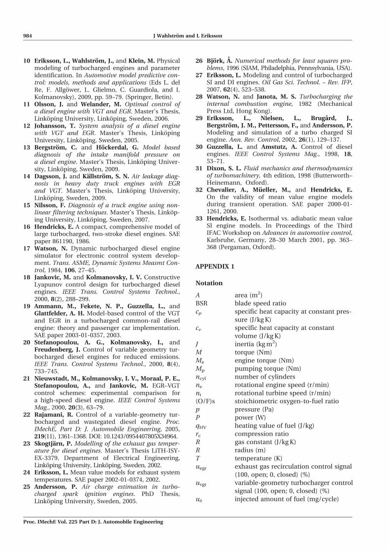
10 Eriksson, L., Wahlstrom, J., and Klein, M. Physicalmodeling of turbocharged engines and parameteridentification. In Automotive model predictive con-trol: models, methods and applications (Eds L. delRe, F. Allgower, L. Glielmo, C. Guardiola, and I.Kolmanovsky), 2009, pp. 59–79. (Springer, Betin).

11 Olsson, J. and Welander, M. Optimal control ofa diesel engine with VGT and EGR. Master’s Thesis,Linkoping University, Linkoping, Sweden, 2006.

12 Johansson, T. System analysis of a diesel enginewith VGT and EGR. Master’s Thesis, LinkopingUniversity, Linkoping, Sweden, 2005.

13 Bergstrom, C. and Hockerdal, G. Model baseddiagnosis of the intake manifold pressure ona diesel engine. Master’s Thesis, Linkoping Univer-sity, Linkoping, Sweden, 2009.

14 Dagsson, J. and Kallstrom, S. N. Air leakage diag-nosis in heavy duty truck engines with EGRand VGT. Master’s Thesis, Linkoping University,Linkoping, Sweden, 2009.

15 Nilsson, F. Diagnosis of a truck engine using non-linear filtering techniques. Master’s Thesis, Linkop-ing University, Linkoping, Sweden, 2007.

16 Hendricks, E. A compact, comprehensive model oflarge turbocharged, two-stroke diesel engines. SAEpaper 861190, 1986.

17 Watson, N. Dynamic turbocharged diesel enginesimulator for electronic control system develop-ment. Trans. ASME, Dynamic Systems Measmt Con-trol, 1984, 106, 27–45.

18 Jankovic, M. and Kolmanovsky, I. V. ConstructiveLyapunov control design for turbocharged dieselengines. IEEE Trans. Control Systems Technol.,2000, 8(2), 288–299.

19 Ammann, M., Fekete, N. P., Guzzella, L., andGlattfelder, A. H. Model-based control of the VGTand EGR in a turbocharged common-rail dieselengine: theory and passenger car implementation.SAE paper 2003-01-0357, 2003.

20 Stefanopoulou, A. G., Kolmanovsky, I., andFreudenberg, J. Control of variable geometry tur-bocharged diesel engines for reduced emissions.IEEE Trans. Control Systems Technol., 2000, 8(4),733–745.

21 Nieuwstadt, M., Kolmanovsky, I. V., Moraal, P. E.,Stefanopoulou, A., and Jankovic, M. EGR–VGTcontrol schemes: experimental comparison fora high-speed diesel engine. IEEE Control SystemsMag., 2000, 20(3), 63–79.

22 Rajamani, R. Control of a variable-geometry tur-bocharged and wastegated diesel engine. Proc.IMechE, Part D: J. Automobile Engineering, 2005,219(11), 1361–1368. DOI: 10.1243/0954407805X34964.

23 Skogtjarn, P. Modelling of the exhaust gas temper-ature for diesel engines. Master’s Thesis LiTH-ISY-EX-3379, Department of Electrical Engineering,Linkoping University, Linkoping, Sweden, 2002.

24 Eriksson, L. Mean value models for exhaust systemtemperatures. SAE paper 2002-01-0374, 2002.

25 Andersson, P. Air charge estimation in turbo-charged spark ignition engines. PhD Thesis,Linkoping University, Sweden, 2005.

26 Bjork, A. Numerical methods for least squares pro-blems, 1996 (SIAM, Philadelphia, Pennsylvania, USA).

27 Eriksson, L. Modeling and control of turbochargedSI and DI engines. Oil Gas Sci. Technol. – Rev. IFP,2007, 62(4), 523–538.

28 Watson, N. and Janota, M. S. Turbocharging theinternal combustion engine, 1982 (MechanicalPress Ltd, Hong Kong).

29 Eriksson, L., Nielsen, L., Brugard, J.,Bergstrom, J. M., Pettersson, F., and Andersson, P.Modeling and simulation of a turbo charged SIengine. Ann. Rev. Control, 2002, 26(1), 129–137.

30 Guzzella, L. and Amstutz, A. Control of dieselengines. IEEE Control Systems Mag., 1998, 18,53–71.

31 Dixon, S. L. Fluid mechanics and thermodynamicsof turbomachinery, 4th edition, 1998 (Butterworth–Heinemann, Oxford).

32 Chevalier, A., Mueller, M., and Hendricks, E.On the validity of mean value engine modelsduring transient operation. SAE paper 2000-01-1261, 2000.

33 Hendricks, E. Isothermal vs. adiabatic mean valueSI engine models. In Proceedings of the ThirdIFAC Workshop on Advances in automotive control,Karlsruhe, Germany, 28–30 March 2001, pp. 363–368 (Pergaman, Oxford).

APPENDIX 1

Notation

A area (m2)

BSR blade speed ratio

cp specific heat capacity at constant pres-

sure (J/kg K)

cv specific heat capacity at constant

volume (J/kg K)

J inertia (kg m2)

M torque (Nm)

Me engine torque (Nm)

Mp pumping torque (Nm)

ncyl number of cylinders

ne rotational engine speed (r/min)

nt rotational turbine speed (r/min)

(O/F)s stoichiometric oxygen-to-fuel ratio

p pressure (Pa)

P power (W)

qHV heating value of fuel (J/kg)

rc compression ratio

R gas constant (J/kg K)

R radius (m)

T temperature (K)

uegr exhaust gas recirculation control signal

(100, open; 0, closed) (%)

uvgt variable-geometry turbocharger control

signal (100, open; 0, closed) (%)

ud injected amount of fuel (mg/cycle)



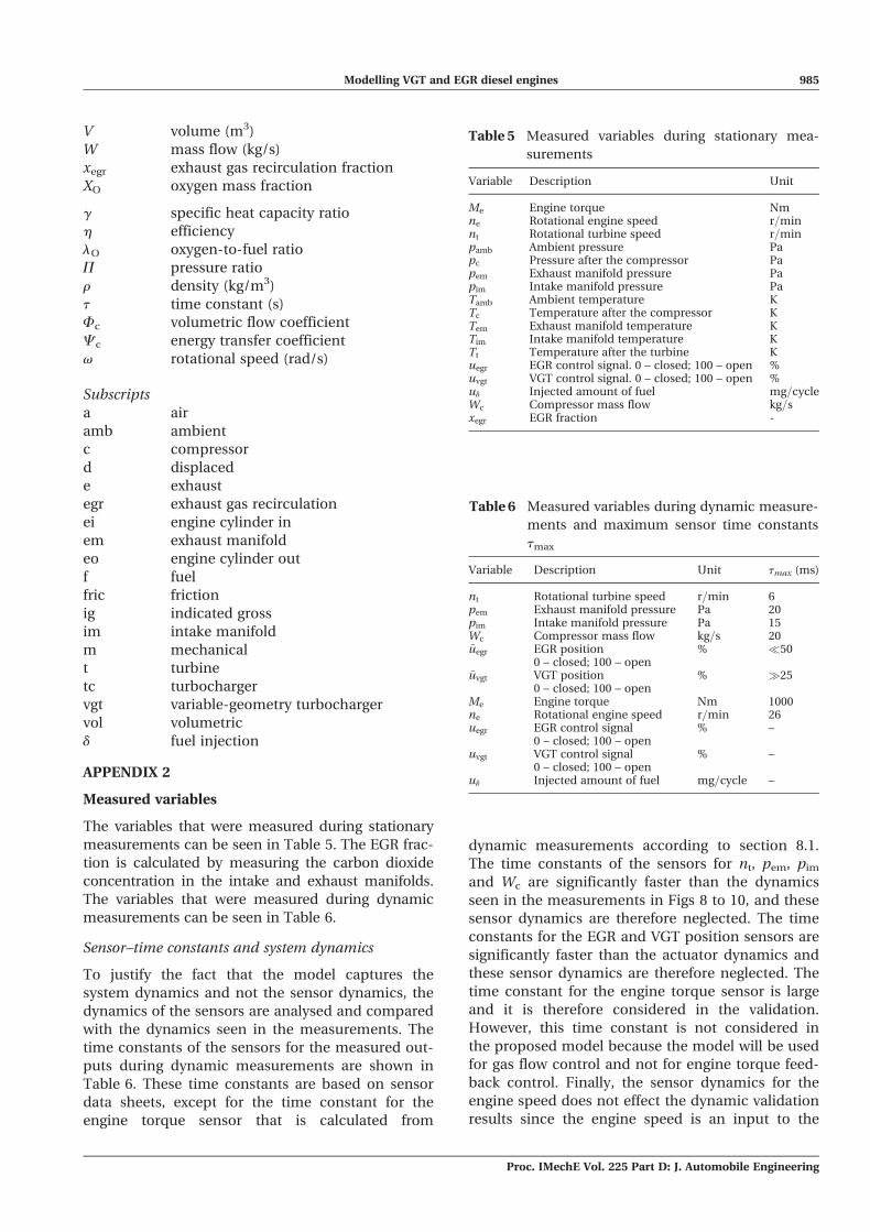
V volume (m3)

W mass flow (kg/s)

xegr exhaust gas recirculation fraction

XO oxygen mass fraction

g specific heat capacity ratio

h efficiency

lO oxygen-to-fuel ratio

P pressure ratio

r density (kg/m3)

t time constant (s)

Fc volumetric flow coefficient

Cc energy transfer coefficient

v rotational speed (rad/s)

Subscripts

a air

amb ambient

c compressor

d displaced

e exhaust

egr exhaust gas recirculation

ei engine cylinder in

em exhaust manifold

eo engine cylinder out

f fuel

fric friction

ig indicated gross

im intake manifold

m mechanical

t turbine

tc turbocharger

vgt variable-geometry turbocharger

vol volumetric

d fuel injection

APPENDIX 2

Measured variables

The variables that were measured during stationary

measurements can be seen in Table 5. The EGR frac-

tion is calculated by measuring the carbon dioxide

concentration in the intake and exhaust manifolds.

The variables that were measured during dynamic

measurements can be seen in Table 6.

Sensor–time constants and system dynamics

To justify the fact that the model captures the

system dynamics and not the sensor dynamics, the

dynamics of the sensors are analysed and compared

with the dynamics seen in the measurements. The

time constants of the sensors for the measured out-

puts during dynamic measurements are shown in

Table 6. These time constants are based on sensor

data sheets, except for the time constant for the

engine torque sensor that is calculated from

dynamic measurements according to section 8.1.

The time constants of the sensors for nt, pem, pim

and Wc are significantly faster than the dynamics

seen in the measurements in Figs 8 to 10, and these

sensor dynamics are therefore neglected. The time

constants for the EGR and VGT position sensors are

significantly faster than the actuator dynamics and

these sensor dynamics are therefore neglected. The

time constant for the engine torque sensor is large

and it is therefore considered in the validation.

However, this time constant is not considered in

the proposed model because the model will be used

for gas flow control and not for engine torque feed-

back control. Finally, the sensor dynamics for the

engine speed does not effect the dynamic validation

results since the engine speed is an input to the

Table 5 Measured variables during stationary mea-

surements

Variable Description Unit

Me Engine torque Nmne Rotational engine speed r=minnt Rotational turbine speed r=minpamb Ambient pressure Papc Pressure after the compressor Papem Exhaust manifold pressure Papim Intake manifold pressure PaTamb Ambient temperature KTc Temperature after the compressor KTem Exhaust manifold temperature KTim Intake manifold temperature KTt Temperature after the turbine Kuegr EGR control signal. 0 – closed; 100 – open %uvgt VGT control signal. 0 – closed; 100 – open %ud Injected amount of fuel mg=cycleWc Compressor mass flow kg=sxegr EGR fraction -

Table 6 Measured variables during dynamic measure-

ments and maximum sensor time constants

tmax

Variable Description Unit tmax (ms)

nt Rotational turbine speed r=min 6pem Exhaust manifold pressure Pa 20pim Intake manifold pressure Pa 15Wc Compressor mass flow kg=s 20~uegr EGR position % �50

0 – closed; 100 – open~uvgt VGT position % �25

0 – closed; 100 – openMe Engine torque Nm 1000ne Rotational engine speed r=min 26uegr EGR control signal % –

0 – closed; 100 – openuvgt VGT control signal % –

0 – closed; 100 – openud Injected amount of fuel mg=cycle –



model and it is also constant in all measurements

used here.

APPENDIX 3

Notes on the contributed model

A MATLAB Simulink implementation of the model

together with a complete parameter file is available

from reference [5] or by contacting the authors. The

intention of this implementation is to give research-

ers and engineers access to a validated model that

can be used for simulation, development, and veri-

fication of new control systems. Researchers

working on methodology development can use this

model as a challenging reference case since it

describes a highly non-linear system with non-

minimum phase behaviour.

Together with the implementation and parameter

files there is also a MATLAB script runSimEngine.m

that simulates the implementation for the two steps

in VGT position shown in Figs 11 and 12, and gen-

erates these two figures for the eighth-order model.

This MATLAB-script illustrates how the implemen-

tation can be simulated and gives examples on two

step responses that have non-minimum phase

behaviour, overshoot, and sign reversal.



Documents

Modelling diesel engines with a variable-geometry …430022/FULLTEXT02.pdfModelling diesel engines with a variable-geometry turbocharger and exhaust gas recirculation by optimization