Embed Size (px)
Citation preview

MODELLING DEFAULT RISK CHARGE (DRC):
INTERNAL MODEL APPROACH
Javier Ojea Ferreiro
Trabajo de investigación 010/016
Master en Banca y Finanzas Cuantitativas
Tutores: Dra. Eva Ferreira
Dr. Gregorio Vargas Martínez
Universidad Complutense de Madrid
Universidad del País Vasco
Universidad de Valencia
Universidad de Castilla-La Mancha
www.finanzascuantitativas.com

Master in Banking and Finance
University of Castilla la Mancha Complutense University of Madrid University of the Basque Country
University of Valencia
Modelling Default Risk Charge
(DRC): Internal Model Approach.
Author: Javier Ojea Ferreiro
Supervisors: Eva Ferreiraa, Gregorio Vargas Martínez
b
a Basque Country University, Barrio Sarriena, s/n, 48940 Leioa, Bizkaia,
España bErnst & Young, Torre Picasso, Plaza de Pablo Ruiz Picasso nº1, 28020
Madrid, Spain
2015/2016

2
Master in Banking and Finance
University of Castilla la Mancha
Complutense University of Madrid
University of the Basque Country
University of Valencia
Modelling Default Risk Charge (DRC): Internal Model Approach.
Authors: Javier Ojea Ferreiro
Supervisors: Eva Ferreiraa, Gregorio Vargas Martínez
b
a Basque Country University, Barrio Sarriena, s/n, 48940 Leioa, Bizkaia, España
bErnst & Young, Torre Picasso, Plaza de Pablo Ruiz Picasso nº1, 28020 Madrid, Spain
Abstract
The Fundamental Review of Trading Book (FRTB), known as Basel 4, introduces
capital requirements for market risk in bank‘s trading book for which is necessary model
default events. The FRTB overhaul trading book capital rules in order to obtain a more
coherent and consistent framework. The main aims of this review of previous Basel
regulation are to consolidate existing measures and to reduce variability in capital level
across banks.
All elements of the new regulation in market risk capital requirements should be fully
tested before framework is introduced. There are several reasons that explain the importance
of modelling and following up the new measures of the regulation hereinabove. Ambiguous
rules about the way of developing models for the new measures can flow into divergence on
domestic rules, so the huge variability across firms could not decrease. Moreover, a lack of
consistency in the model could lead on an inappropriate high capital levels for some
business lines that will reduce liquidity and increase cost for end users and, as a
consequence, in this scenario some business lines will become uneconomic. There are two
approaches in capital requirements of Basel 4: standardized approach and internal model
approach. This article focuses in a specific measure under de internal approach: the Default
Risk Charge measure.
Keywords: Fundamental Review of the Trading Book, Default Risk Charge, Market Risk

3
Index 1. Motivation ..................................................................................................................... 8
2. Regulation background .................................................................................................. 10
2.1. Basel I .................................................................................................................. 10
2.2 Basel II ................................................................................................................. 10
2.3 Basel 2.5 ............................................................................................................... 11
2.3.1. Shortcomings ................................................................................................. 11
2.4. Basel 4 ................................................................................................................. 14
2.4.1. The revised boundary between trading book and banking book ............................. 14
2.4.2. The revised standardized approach .................................................................... 15
2.4.3. The revised internal models approach ................................................................ 15
3. Default Risk Charge as a risk measure ............................................................................. 18
3.1 Definition ............................................................................................................. 18
3.2. Goals .................................................................................................................... 21
3.3. Challenges ............................................................................................................ 22
4. Default Risk Charge: a model approach ........................................................................... 24
4.1. Exposure At Default (EAD) .................................................................................... 24
4.1.1. Making the EAD uniform between SA and IMA. ................................................ 24
4.1.2. Long/ short definition ...................................................................................... 25
4.1.3. EAD and CVA ............................................................................................... 25
4.2. Marginal PD .......................................................................................................... 25
4.2.1. Types of PD ................................................................................................... 26
4.3. Default across obligors ........................................................................................... 28
4.3.1. Types of credit risk models .............................................................................. 28
4.3.2. Comparison: IRB vs. DRC default simulation model ........................................... 29
4.3.3. Proposed model .............................................................................................. 31
4.3.3.4. Quantile regression ...................................................................................... 43
4.3.4. Simulation process .......................................................................................... 45
4.4. LGD model ........................................................................................................... 47
4.4.1. Requirements for the Loss Given Default by the FRTB and empirical evidence ...... 48
4.4.2. Most important stochastic distribution for modeling LGD studied in the literature .. 50
4.4.3. Proposed model .............................................................................................. 51
5. Empirical analysis ......................................................................................................... 53
5.1. Data ..................................................................................................................... 53
5.1.1. Portfolios ....................................................................................................... 56
5.2. Algorithm ............................................................................................................. 58

4
5.2.1. Parallel Computing technique ........................................................................... 59
5.3. Parameter sensitivity .............................................................................................. 61
5.3.1. Different levels of quantiles and the influence of the global factor in the recovery rate 62
5.3.2. Changes in the probabilities of default ............................................................... 63
5.3.3. Changes in the influence of the global factor in the recovery rate .......................... 64
5.3.4. Study about the different estimation methods ..................................................... 65
5.4. Variance reduction techniques ................................................................................. 69
5.4.1. Antithetic Variates .......................................................................................... 69
5.5. Further consideration: copulas ................................................................................. 71
6. Conclusion ................................................................................................................... 73
7. References ................................................................................................................... 75
8. Appendix ..................................................................................................................... 82
8.1. Appendix of tables ................................................................................................. 82
8.2. Appendix of figures ................................................................................................ 92

5
Equation 1: General expression for the default triggered equation following Wilkens and
Predescu (2015) ................................................................................................................ 31
Equation 2: Asset-value changes under a similar metric that follows Pykhtin (2004) ......... 32
Equation 3: Relation between systematic factors and the composite factor ....................... 33
Equation 4: Asset default correlation ................................................................................. 33
Equation 5: Default triggered equation under Gaussian copula ......................................... 35
Equation 6: Clayton copula density function ...................................................................... 38
Equation 7: Hierarchical nested multivariate copula for the asset returns simulation ......... 38
Equation 8: Default triggered equation under a nested copula which employs Clayton
copula and Gaussian in a upper level ................................................................................ 39
Equation 9: Equicorrelation matrix form ............................................................................. 40
Equation 10: Inverse of an equicorrelation matrix .............................................................. 41
Equation 11: Determinant of an equicorrelation matrix ....................................................... 41
Equation 12: Maximization of the log-likelihood for getting the parameter of the
equicorrelation matrix ........................................................................................................ 41
Equation 13: Maximization of the log-likelihood explicit form for getting the parameter of the
equicorrelation matrix ........................................................................................................ 42
Equation 14: Regression of the asset in order to obtain the weights for equation (5) ......... 43
Equation 15: minimization of the absolute error following a quantile regression ................. 44
Equation 16: Simulation of the composite factor ................................................................ 46
Equation 17: Inverse conditional Clayton copula ................................................................ 47
Equation 18:copula distribution parameters estimation using ML under the supposition of
the normal marginal distributions ....................................................................................... 47
Equation 19: Latent variable of the recovery rate ............................................................... 51
Equation 20: recovery rate approach ................................................................................. 51

6
Figure 1: Structure of a two-level nested copulas with normal marginal distribution ........... 92
Figure 2: DECO correlation from 1995-2005 across the main stock market indexes. ......... 92
Figure 3: Regression simulated under OLS and different quantile regressions .................. 93
Figure 4: Regression simulated under OLS and different quantile regressions (detail) ...... 93
Figure 5: Residuals and weight for the residual under each different regression employed 94
Figure 6: Country of the equity from Eurostoxx employed in the sensitivity analysis .......... 95
Figure 7: Rating of the equity from Eurostoxx employed in the sensitivity analysis ............ 96
Figure 8: Sector of the equity from Eurostoxx employed in the sensitivity analysis ............ 96
Figure 9: Correlation default distribution of corporate and sovereign assets ...................... 97
Figure 10: Correlation default distribution of corporate assets using a country systematic
factor ................................................................................................................................. 97
Figure 11: Correlation default distribution of corporate assets using a industry systematic
factor ................................................................................................................................. 98
Figure 12: Number of defaults depending on the chosen second systematic factor ........... 98
Figure 13: LGD for NUMERICABLE SFR using different values for the parameter of
influence of the global factor in equation (19) .................................................................... 99
Figure 14: Different VaR depending on the quantile of the regresion and the influence of the
global factor in the recovery rate for a portfolio made of corporate debt using country as a
second systematic factor. ................................................................................................ 100
Figure 15: Different VaR depending on the quantile of the regresion and the influence of the
global factor in the recovery rate for a portfolio made of corporate debt using industry as a
second systematic factor. ................................................................................................ 101
Figure 16: Estimated parameters test (q=0.2 regression against OLS regression) for BBVA
returns using country (upper)or sector (lower) as a second factor.................................... 102
Figure 17:Estimated parameters test (monthly against quarterly data employed to a q=0.2
quantile regression) for BBVA returns using country (upper)or sector (lower)as a second
factor ............................................................................................................................... 103
Figure 18: DRC of the different portfolios and the increase if a Clayton copula is employed
in the systematic factors .................................................................................................. 104

7
Table 1: Values of alpha and beta for the beta distribution ................................................ 83
Table 2: Probability of default obtained from Wilkens and Predescu (2016) ....................... 83
Table 3: Assets employed in the empirical exercise ........................................................... 88
Table 4: Change in the DRC (%) if the probabilities of default decrease a basis point ....... 89
Table 5: Change in the DRC (%) if the probabilities of default increase a basis point ........ 89
Table 6: Change in the DRC (%) if the influence of the global factor in the reocvery is
different from 0.5 ............................................................................................................... 89
Table 7 : Change in the DRC (%) if the OLS values of the parameters are employed........ 90
Table 8: Change in the DRC (%) if the quarterly data is employed .................................... 90
Table 9: Change in the DRC (%) a Clayton copula is employed in the systematic factors . 90
Table 10: Initial DRC values for the portfolios .................................................................... 90
Table 11: Mean of the values of VaR using plain MC and antithetic MC ............................ 90
Table 12: Variance of the values of VaR using plain MC and antithetic MC ....................... 91

8
1. Motivation "The fault, dear Brutus, is not in our stars,
But in ourselves, that we are underlings."
Julius Caesar, Act I, Scene III, L. 140-141
A consistent framework for the financial regulation and cautious measures for the risk
of the financial institutions are one of the most important goals of the economic science. In
order to be aware of this, the analogy that Édouard Daladier1 made between the financial
system and the human body could be quite explanatory. While the heart pumps the blood
into the different part of the body, the financial system injects liquidity into the different
sectors of the economy, and a failure in any of them could be mortal.
Historically, when the financial structure has been built on weak pillars the
consequences that have been suffered were outrageous. The results have been reflected in
our cultural background inspiring books and films such as The Graves of Wrath where
Steinbeck reveals the consequences of an appalling financial regulation and the lack of
awareness of the risks that banks had taken in the previous decade. The financial crisis
inquiry report of United States published in 2011 tries to raise awareness of the importance
of the financial regulation, pointing out that the subprime crisis had not been consequence of
an awful fortune, but it had been the result of not paying enough attention to the risk
positions that the financial sector had begun to take. The quote of Shakespeare that opens
this introduction hits in the target of this idea. This idea motivated the recent review of the
bank regulation guidelines proposed by the Basel Committee and known as the FRTB
(Fundamental Review of Trading Book) or Basel 4. This idea also impregnates the present
thesis in order to get a right model approach for a particular measure called Default Risk
Charge (DRC).
The aim of this Master‘s thesis is focused on comparing different methodological
approaches, always having concern of the recommendation made by the Committee, and
given some assumptions studying the variability of the DRC measure. More precisely, this
Master‘s thesis is structured in four chapters.
The following chapter analyzes the meaning of market risk in management and as
regulation capital. Therefore in this part of the article the evolution of market risk capital
requirement is handled in the different approach that Basel Committee on Banking 1 Édouard Daladier was the French prime minister in the early thirties.

9
Supervision has applied over time and the reasons that explain the enhancement of the
measures until the nowadays regulation.
Chapter 3 introduces a broadly concept of the DRC, its goals and challenges. Chapter
4 introduces DRC measure under the perspective of the internal model approach, taking into
account the requirements with the purpose of modeling the DRC. This chapter is, at the
same time, subdivided into two parts. The first part is oriented at modeling probabilities of
default while the second part is focused on assessment of loss given default under different
models. The goal of this section is to regard different ways of generate a P&L (profit and
loss) distribution that would allow to perform the assessment of the DRC.
Chapter 5 is connected with chapter four; due to this is an empirical approach of the
different methods to calculate DRC measure presented in chapter 3 given some portfolios.
Finally, chapter 6 outlines the main ideas of the article and sum up the objectives of
this measure, challenges and possible lines of work that could be developed.

10
2. Regulation background
2.1. Basel I An accurate economic regulation is one of the main requirements to allow a
sustainable economic growth. The existence of moral hazard and other market failures make
essential regulation in financial field. Basel commitments are the backbone of overarching
financial regulation. Basel I commitment in 1988 was the first major step in addressing
regulation of internationally active banks. Unfortunately, Basel I suffered from its limited
scope. The exclusion of market and operational risk in Basel I can serve as proof of the lack
of scope of this first approach to bank regulation guidelines. Market risk can be defined as
the risk of losses in on and off-balance sheet positions arising from adverse movements in
market prices, while the operation risk can be understood as the risk of loss resulting from
inadequate or failed internal processes, people and systems, or for external events.
Bank‘s regulation is always triggered by shocks and recessions that bring weaknesses
out. In Basel, the introduction of capital requirements for market risk was the consequence
of the collapse of Barings in 1995. The result was the 1995/1996 market risk amendment to
Basel I. This bankruptcy clears up the importance of market risk that was out of the scope of
the initial Basel proposal. The assessment of market risk in Basel included all instruments in
the trading book including those that were out of balance sheet, and was focused on internal
models developed by own institutions in order to manage the risks that they had taken.
2.2 Basel II Basel I commitment quickly became outdated due to its simplicity that did not take
into account the existence of bank guarantee neither distinguish the risk firm profile when
the capital was fixed. Basel II commitment began to negotiate in 1999 and is finally
published in 2006. The structure of capital regulation framework increased thanks to this
review of bank‘s guideline regulation. Basel II was built on three pillars: minimum capital
for credit, market and operational risk, a supervisor process both internal as self-assessment
and external that oversaw the perform of the firm, and disclosed information in order to let
market discipline reward banks that carry out a sensible criteria management. Basel II
furthered in terms of self-regulation, allowing banks to assess their own risks, as a result of

11
developing an internal approach for sophisticated banks that requires complex and advanced
estimation methodologies.
The review of Basel II arose as a consequence of the series of shortcomings displayed
by the 2008 financial crisis in the aftermath of Lehman Brothers collapse. The insufficient
capital requirement for trading book exposures prior to the 2007-2008 period of the financial
crisis was in part responsible for the difficulties that some firms suffered. An ambiguous
definition of the regulatory boundary between the banking book and the trading book left the
way open to regulatory capital arbitrage in order to reduce the financial buffer of capital for
unexpected losses fixed by the regulation. In addition, risk measurement methodologies
were not sufficiently robust. In fact, internal models for market risk requirements relied on
risk drivers determined by banks, which has not led to sufficient capital for the banking
system as a whole. The main difference between both books is that trading book is hold for
speculation proposes while banking books consist of portfolios that are supposedly hold
until maturity.
2.3 Basel 2.5 The Basel 2.5 reforms included requirements for banks to hold additional capital
against default and rating migration risks, and also required banks to calculate an additional
value-at-risk (VaR) capital charge in stressed economic conditions, in order to alleviate the
inadequate capital requirement established by the previous regulation. This reform published
in 2009 also removed most securitization exposures form internal models due to the lack of
model‘s robustness for these assets, and required such exposures to be treated as if held in
the banking book.
2.3.1. Shortcomings In spite of the set of revisions to the market risk framework that was introduced by the
Basel Committee as part of the Basel 2.5 package of reforms, a number of structural flaws in
market risk framework remained unaddressed. That is the reason why on January 2016, the
Basel Committee on Banking Supervision (BCBS) published its revised capital requirements
for market risk, also known as the Fundamental Review of the Trading Book (FRTB). The
FRTB looks for mitigate the flaws that Basel 2.5 did not fixed correctly.

12
2.3.2. Boundary between trading book and banking book
The regulatory boundary between books was not fully specified in Basel 2.5. The
Basel Committee made only minor amendments to the specification of instruments that
should be excluded from, or included in, the trading book. Subjective criterions of banks
were key determinant when a portfolio had to be associated to trading or banking book, so
capital arbitrage continued. The new boundary between the trading book and banking book
will limit the potential for regulatory arbitrage. The FRTB has stringent rules for internal
transfers between trading and banking book with the purpose of eliminating capital
arbitrage. In order to achieve this goal, a list of assets that should be placed in the trading
book is also specified, and unless a justifiable reason that must be its place. Moreover, new
regulation will limit the institution‘s ability to move illiquidity assets from its trading book
to its banking book. Furthermore, if the capital charge on an instrument is reduced as a
consequence of a movement of this instrument between books. The difference charge
measured in the switching is imposed as a fixed, additional and disclosed capital charge. The
Basel Committee on Banking Supervision has designed this range of measure to reduce
incentives for arbitrage between the regulatory banking and trading books.
2.3.3 Flaws of VaR-type measure
Another example of the drawbacks of the Basel 2.5 reform was the weaknesses that
VaR-type measures framework presented. The VaR metric does not correctly capture
exposures to some risks and also creates wrong incentives as the result of being focus just in
a percentile of the profit and loss (P&L) distribution. Particularly, the fact that VaR measure
is not subadditive implies that the diversification is penalized.
The VaR-based metric used to capitalize trading book exposures was inadequate for
capturing credit risk inherent in trading exposures. The hasty growth in the market for traded
credit implied that banks held large exposures to undercapitalized credit-related instruments
in their regulatory trading book. Also market illiquidity was inadequately captured, due to
the fact that previous framework made the assumption that banks can exit or hedge their
trading book exposures over a 10-day period without affecting market prices. However,
when the banking system holds similar exposures in traded instruments, the market where
those instruments are traded is likely to quickly turn illiquid in times of stress, as 2008
financial crisis shows us. In FRTB framework, the concept of liquidity horizon is
introduced, that can be defined as the time required to exit or hedge a risk position without
materially affecting market prices in stressed market conditions.

13
The VaR-based framework just takes in consideration a percentile, without looking
beyond that percentile, as a consequence this measure fails to capture ―tail risks‖. Ohran and
Karaahmet (2009) found out that VaR performs correctly when the economy experiment
smoothly moves, but fails during times of economic stress, because VaR hasthe feature of
being insensitive to the size of loss beyond the pre-specified threshold. For instance, in the
pre-crisis phase, providing insurance against certain tail events was recognized as a ―risk-
less‖ strategy according on prevailing regulatory capital requirements at that time. Large
unexpected losses when these tail events have occurred emanate from this incorrect use of
VaR measure.
VaR measure has received generalized criticism due to its drawback that is
consequence of paying attention just in a certain percentile. Artzner, Delbaen, Eber, & Heath
(1999; 1997) stand out the lack of sub-additivity as the most notable flaw of this measure,
whereas Pflug (2000) point out that Conditional Value at Risk (CVaR), also known as
Expected Shortfall does not have this inconvenient property by dint of looking at losses
beyond VaR. This is the main reason why previous most of VaR measures of Basel 2.5 are
changed by CVaR measures in Basel 4, with the exception of DRC model.
In the FRTB initiative is exposed a new and costly measure to capture internal models‘
tail risk. The final framework replaces Value at Risk (VaR) and Stressed VaR (SVaR)
measures for capturing risk with the Expected Shortfall (ES). This ensures capture of tail
risks that are not accounted for in the existing VaR measures, and that implies higher capital
requirements under the final framework. Furthermore, tail risk capture comes at a significant
cost, as data requirements and operational complexities of the ES measure are likely to be
extensive.
2.3.3. Excessive recognition of diversification benefits
Under the Basel 2.5 framework there were generous recognition of the risk-reducing
effects of hedging and diversification, due to the fact that the estimation of correlations
derived from historical data under ―normal‖ market conditions. Hedging benefits proved
illusory as correlation assumptions broke down over periods of market stress. The revised
framework establishes that ES must be calibrated to a period of significant financial market
stress. Moreover, a series of changes under the revised regulation serve to constrain the
capital-reducing effects of hedging and diversification in the internal models approach. The
ES capital charge for modellable risk factors does not allow unconstrained recognition of
diversification benefits, but limited the cross-risk class diversification benefits.

14
2.3.4. Lack of sensitivity of the standardized approach
Additionally, under the Basel 2.5 regulation framework, the standardized approach
was not a credible fallback to the internal models approach, because it does not embed a
clear link between the models-based and standardized approaches either in terms of
calibration or the conceptual approach to risk measurement. Moreover, standardized
approach endures a lack of risk sensitivity and insufficient capture of risks associated with
complex instruments. Nipping these weaknesses of the design of the current framework in
the bud is one of the main aims of the FRTB initiative. The revised standardized approach
for market risk based on price sensitivities, which is intended to be more risk sensitive
compared to the existing standard approach, and therefore reduce the gap between internal
models and standard rules. It provides a fallback in the event that bank‘s internal model is
deemed inadequate, including the use as a floor to an internal models-based charge. The
framework‘s requirements are clearly designed to push firms towards the new standardized
approach, which is consistent with the overall regulatory trend of moving away from
internal model-based approaches. This idea is bolstered by the framework‘s more stringent
requirements applicable to the use of internal models.
2.4.Basel 4 At this point, regulatory background is clearly exposed as a process of continuous
enhancements driven by shocks and financial crisis up to the following regulation reform
that nowadays is being published, the Fundamental Review of Trading Book (FRTB), also
known as Basel 42. The revised capital standard for market risk is focused on three key
areas: the revised boundary between trading book and banking book, the revised
standardized approach and the revised internal models approach.
2.4.1. The revised boundary between trading book and banking book
As stated above, FRTB imposes strict limits to firms‘ ability to move instruments
between books, enhancing supervisory powers and reporting requirements. What is more,
clearing which instruments should be stayed in each book and the treatment of internal risk
transfers across the regulatory boundary. Nevertheless, it is not clear that the revised
2Basel 3 framework focused on capital, liquidity ratios (LCR, NSFR), Leverage ratio and counterparty
credit risk modeling while Basel 4 focused on market risk.

15
boundary will be effective in reducing such capital arbitrage positions in all jurisdictions due
to that national regulators are given discretion in defining their instruments lists.
2.4.2. The revised standardized approach Concerning the revised standardized approach (SA), the overhaul seeks a risk-
sensitive measure that can be useful as a credible fallback and floor to the internal model
approach (IMA), while sophisticated treatment for market risk is not required under this
approach.
2.4.2.1. The sensitivities based Method
The main components of the standardized capital requirement in the trading book are
the followings. The Sensitivities Based Method tries to capture ―delta‖, ―vega‖ and
―curvature‖ risks, extending the use of sensitivities to a much broader set of risk factors than
current framework. These risks are related with changes in the instruments in relation to the
underlying, the implicit volatility and the changes in the delta in relation to the underlying
respectively.
2.4.2.2. The default risk charge (DRC)
The second component of the SA is the default risk charge (DRC). The aim of this
measure is to reduce the potential discrepancy in capital requirements for similar risk
exposures across the banking book and trading book. It is a floor and a fallback for the IMA
default risk charge when the bank‘s supervisory authority does not approve explicitly this
last one. Moreover DRC standardized approach must be applied for exposure in the trading
book.
2.4.2.3. The residual risk add-on
The third component of the standardized approach is the residual risk add-on that
captures any other risks beyond the main risk factors already captured in the two previous
components. It provides for a simple and conservative capital treatment for
complex/sophisticated instruments that would otherwise be inaccurately captured.
2.4.3. The revised internal models approach Finally, regarding the internal model approach (IMA) capital requirements for non-
securitizations in the trading book, the total capital requirement would be the sum of

16
Expected Shortfall (ES), the DRC and stressed capital add-on (SES) for non-modellable
risks.
2.4.3.1. Expected Shortfall (ES)
The use of a Global Expected Shortfall (ES) is made up of equally weighted average
of diversified ES and non-diversified partial ES capital charges for specified risk classes.
Expected Shortfall should be calculated as the expected losses of a portfolio
conditional to the fact that the loss is greater than the 97.5th percentile of the loss
distribution. 3This risk measure must be computed on a daily basis and at a base liquidity
horizon of ten days.4
2.4.3.2. The default risk charge (DRC)
In addition to this measure, DRC captures default risk of credit and equity trading
book exposures with no diversification effects allowed with other market risks (including
credit spread risk). A default risk measure in the capital requirements for market risk could
be rather confusing given the fact that might be associated with credit risk in a first glance.
Traditionally, trading book portfolios consisted of liquid positions easy to trade or hedge.
However, developments in banks‘ portfolios have led to an increase in the presence of credit
risk and illiquid positions not suited to the original market capital framework. That is the
reason why, a measure as DRC, or the previous Incremental Risk Charge (IRC), is essential
in order to address these flaws in the traditional understanding of market risk.
Despite the fact that both DRC and IRC are designed to capture default risk, DRC is
an enhanced measure of the IRC, correcting some flaws that IRC, a measure of Basel 2.5,
had presented. IRC dealt with long term changes in credit quality and in its application huge
discrepancies in risk measures had emerged. The variability of market risk-weighted assets
was that the more complex IRC models were a relatively large source of unwarranted
variation. In response, the revised framework replaces the IRC with a DRC model, in other
words, IRC was transformed in favour of a default-only risk capital charge without a
migration feature, because it was an important source of variation. These changes are good
news for the industry because it prevents from double-counted credit migration risk that in
the Basel 2.5 framework is counted once as part of credit risk volatility and once as a stand-
3Minimum capital requirements for market risk-BCBS (2016) Chapter C, Section 3, paragraph 181
(b) 4Minimum capital requirements for market risk-BCBS (2016) Chapter C, Section 3, paragraph 181
(a) and (c)
17
alone modeled risk. Even though the undeniable superiority of DRC over IRC, the DRC
measure introduces a series of new challenges as the modeling of a big number of issuers
with low correlation as a result of the mandatory inclusion of equity products.
2.4.3.3. The stressed capital add-on (SES) for non-modellable risks
Lastly, Stressed capital add-on aggregates regulatory capital measure for non-
modelable risk factors (NMRF) in model-eligible desks. This component creates incentives
for banks to source high-quality data due to the fact that NMRF are subject to a conservative
capital add-on. In the end, banks will need more data and stronger data analysis to meet the
new risk measurement and reporting requirements. There will be a high cost of risk
measures assessment, given the fact that the ES measure has operational complexities and
the enormous data requirements.
To sum up, the current framework is not based on any overarching view on how risks
from trading activities should be categorized and captured to ensure that the outputs reflect
credible and intuitive capital outcomes. The Fundamental Review of the Trading Book
overhauls trading book capital rules with a more coherent and consistent framework.

18
3. Default Risk Charge as a risk measure
3.1 Definition Default Risk Charge is conceived as a measure to capture default risk of credit and
equity trading book exposures with no diversification effects allowed with other market
risks (including credit spread risk). This stiffness in the lack of diversification effects
allowed with other market risks is due to the huge variability that previous measure,
Incremental Risk Charge (IRC), presented. Choosing the migration feature in order to deal
with changes in credit quality has entailed discrepancies in risk measures, causing huge risk
weight asset variability across financial firms. Since 2012, the Basel Committee on Banking
Supervision (FRTB) has being working on the update of the market risk global regulatory
framework, transforming the IRC in favor of a default-only risk capital charge named DRC5.
Moreover, additional differences with IRC are that DRC measure is extended to equity
position and that a constant portfolio is assumed. The most relevant consequence of
assuming a constant portfolio is that any benefit from recognizing a dynamic hedging
strategy is denied.
The DRC tries to capture stress event in the tail of the default distribution, which may
not be captured by credit spread shocks in mark-to-market risk. So the DRC measure gives
different information from that one provided by credit spread risk. Due to the relationship
between credit spread and default risk banks must seek approval for each desk with
exposure to these risks, otherwise affected desk will be subject to the standardized capital
framework.6
The default risk charge is wished-for to capture jump-to-default risk. The jump-to-
default risk of each instrument is a function of notional amount (or face value) and market
value of the instruments and the Loss Given Default (LGD)7. The default risk is the risk of
direct loss due to an obligor‘s default as well as the potential for indirect losses that may
arise from a default event.8 These inputs are useful to obtain a profit and loss distribution
5In the FRTB consultative papers define the Incremental Default Risk measure, finally was called
Default Risk Charge 6Minimum capital requirements for market risk-BCBS (2016) Chapter C, Section 8, paragraph 186 (r)
7Loss Given Default is understood as one minus recovery rate.
8Minimum capital requirements for market risk-BCBS (2016) Chapter C, Section 8, paragraph 186
(a)

19
(P&L) on the exposure, understanding P&L as cumulative mark-to-market loss on the
position.
In the internal model approach (IMA) DRC can be defined as a VaR-type measure at
99.9% level of confidence and a one-year horizon. However in the case of equity sub-
portfolios a minimum liquidity horizon of 60 days can be applied9. Concerning the risk
horizon, it is necessary to point out the difference between the capital horizon and the
liquidity horizon. Although the capital horizon for regulatory capital is set to one year, banks
are allowed to specify different liquidity horizons or holding periods for instruments such as
equity. For instance, for equity sub-portfolios do not seem to be adequate to assume that the
portfolio will remain constant over a period like one year. That means that if the liquidity
period is chosen shorter than one year, banks must assume that the risk during successive
liquidity periods within the one-year capital horizon is identical. In other words, the constant
portfolio assumption for equity portfolio is just supported during three months, and between
three months period within the one-year capital horizon, a constant level of risk approach is
allowed. Summing up, in the case of the portfolios, a minimum period is set to three months
for the liquidity horizon whereas the capital horizon is always one year.
This issue has been developed in Martin et al (2011) and also Klaassen and Van
Eeghen (2009) referring to the previous risk measure, the Incremental Risk Charge (IRC).
Summing up, a constant position approach of one year is made for the main assets while for
equity assets the constant position approach is reduced to three months, allowing using a
constant level of risk approach after these three months. In practice, this approach could be
setup employing a geometric scaling to obtain the default probability for each period. For
instance, for a three-month period the probability of default for a given asset could be
assessed as 𝑃𝐷𝑡ℎ𝑟𝑒𝑒 𝑚𝑜𝑛𝑡 ℎ𝑠 = 1 − 1 − 𝑃𝐷𝑎𝑛𝑛𝑢𝑎𝑙 1
4. So in the case of a liquidity period
lower than the capital horizon, a multistep model could be employed. The chance of
changing the composition of the portfolio in order to keep stable the level of risk is the main
advantage of using a liquidity period lower than the capital horizon. On the other hand the
most important drawback is the possible unhedged positions (as a consequence of changing
the composition of the portfolio.
There are some flaws in the choice of the constant level approach that have been
analyse in Algorithmics (2009) about the IRC measure that could be extrapolate to the DRC
case. For instance, the multi-period models are inappropiated if they do not preserve the 9Minimum capital requirements for market risk-BCBS (2016) Chapter C, Section 8, paragraph 186
(b)
20
historically observed annual correlations. Multi-period models implicitly reduce the
correlations when roll-overs are modeled. Any modeled rebalancing of the portfolio adds
―noise‖ to a continuous process over time. This effect of reducing the correlation between
obligors as the number of steps in simulation increases is known as ―correlation wash-out‖.
An additional issue of multi-period models is the current contradiction from the principles of
utility theory. As a consequence of the default losses, a bank should reinvest the same dollar
amount into an identical level of risk asset. However, due to the losses, the investment is
now a higher percentage of the wealth of the bank, so the firm is willing to take more risk
for the same reward. In technical terms, assuming a constant level of risk entails a
decreasing marginal utility of wealth as wealth goes down, which contradicts a fundamental
axiom for the utility theory. Moreover, the concept of reinvesting at the same level risk
should be questioned as a feature that is not realistic in ―tail events‖ conditions. In other
words, the constant level of risk assumption is not a reliable feature in the context of
extreme markets, due to the fact that in this kind of situations capital preservation and de-
leveraging is the generalized industry‘s behavior. According to Martin et al (2011) neither of
the two approaches is superior per se, so for the purpose of the article, a constant portfolio
approach is employed.
The combination of the constant level of risk assumption, in the case of equity, and the
one-year capital horizon reflects supervisors‘ assessment of the appropriate capital needed to
support the risk in the trading portfolio. It also reflects the importance to the financial
markets of banks having the capital capacity to continue providing liquidity to the financial
markets in spite of trading losses. Consistent with a ―going concern‖ view of a bank, this
assumption is appropriate because a bank must continue to take risks to support its income-
producing activities. For regulatory capital adequacy purposes, it is not appropriate to
assume that a bank would reduce its VaR to zero at a short-term horizon in reaction to large
trading losses.10
Value at Risk (VaR) is a fundamental tool for managing market risks. It measures the
worst loss to be expected of a portfolio over a given time horizon under normal market
conditions at a given confidence level. The VaR assessment must be done weekly and the
default risk charge model capital requirements is the maximum between the average DRC
10
Guidelines for computing capital for incremental risk in the trading book - BCBS (2009) Chapter II, Section B, paragraph 15

21
measures over the previous twelve weeks (i.e. three months) and the most recent DRC
assessment.11
The measure that focuses this article is a market risk measure, even though it is based
on a dependent credit metric. A measure that tries to capture default risk in a market risk
framework can be rather confusing in a traditional way of understanding trading book
portfolios, where are composed by liquid assets that are easily hedged or traded.
Nevertheless, in nowadays banks‘ portfolios are presenting credit risk and illiquid positions
not suited to the original market capital framework. In this scenario is where measures as
DRC can be understood in a market risk framework.
The instruments that are included to calculate P&L in order to set up DRC measure are
all those which are not subject to standardized DRC (as is the case of non-securitization
position) and whose valuation do not depend solely on commodity prices or foreign
exchange rates. However, this last explicit consideration is just considerer in the 2013
Consultative Document12, while in the capital requirements for market risk published by the
Committee in early January 2016 has been suppressed. Besides, sovereign exposures
(including agencies that are explicitly backed by the government), equity positions and
defaulted debt positions must be included in the model. In relation to equity positions, the
default of an issuer must be modeled as resulting in the equity price dropping to zero13 and,
as a consequence, the recovery rate is assumed zero.
3.2. Goals The DRC model has the goal of correct the main drawback of the IRC measure,
reducing the VaR variability. To achieve this aim, the risk of migration deterioration is not
considered in the measure, because the migration feature was a source of variation.
Furthermore, constrains on the modeling choices for internal model, limiting them to a two-
11
Minimum capital requirements for market risk-BCBS (2016) Chapter C, Section 8, paragraph 186 (d) 12
Basel Committee on Banking Supervision (2013), Fundamental Review of the Trading Book. A Revised Market Risk Framework, Consultative Document, October. Annex 1, Chapter C, Section 8, paragraph 186 (c) 13
Minimum capital requirements for market risk-BCBS (2016) Chapter C, Section 8, paragraph 186 (c)

22
factor model correlation, are looking for reducing also the variability14. Apart from this,
factors of default correlation must be based on listed equity or CDS (Credit Default
Swap).15.
3.3. Challenges The most important challenges that this new measure bring along are the model risk
due to the high confidence level of the risk measure and the long horizon, the disparities
among correlation matrices because of the use of factors based on equity prices or CDS and
the cliff effect along others. The cliff effect is called to the variation on the assessment that
the measure can suffer as a consequence of small changes in the value of the exposure or
other parameters (default probability for instance). An additional challenge is the
questionable use of large pool approximation due to the features of the trading book
positions such as actively traded positions, the presence of long-short credit risk exposures
and potentially small and heterogeneous number of positions. Large pool approximation is
referred to the assumption in the Vasicek loss portfolio distribution model that the basket of
asset that compounds the portfolio is large and homogeneous enough to be considered as a
perfectly diversified portfolio of identical assets. The consequence is that given the
systematic factors, the loss of the portfolio is defined by the level of conditional default risk.
It is remarkable to point out that the Basel Committee has published a consultative
document in March 2016 about the IRB (Internal Rating Based) approach, where some
proposes are presented in order to improve this approach for determining the regulatory
capital requirements for credit risk.16The most outstanding propose, that could affect our
measure, is the recommendation of avoid using internal approach for exposures where the
model parameters cannot be estimated sufficiently reliably for regulatory purposes, like
banks and other financial institutions, large corporate and equities. For instance, in our
article there is a lack of information about recovery rates for sovereign bonds due to the fact
that it is a very unusual event, as a consequence the Loss Given Default could be inadequate
measured and this could be the cause of a persistent high variability in this kind of VaR-type
14
Minimum capital requirements for market risk-BCBS (2016) Chapter C, Section 8, paragraph 186 (b) 15
Minimum capital requirements for market risk-BCBS (2016) Chapter C, Section 8, paragraph 186 (b) 16Reducing variation in credit risk-weighted assets – constraints on the use of internal model approaches. Consultative Document. BCBS (2016) Chapter 2

23
measure. This recommendation for credit risk measures could be inconsistent with the DRC
measure due to the fact that low probability of default portfolios could lead to a DRC‘s
assessment under the internal approach but in IRB approach is not proposed by the
Committee, when both kinds of measures analyzed the default risk.
24
4. Default Risk Charge: a model approach
In this second chapter, an approach modelling for the DRC measure is proposed,
always taking into account the requirements that the Basel Committee required for the
internal approach. There are three main issues in this chapter concerning loss due to a
default event: Exposure At Default (EAD), Probability of Default (PD) and the Loss Given
Default (LGD).
4.1. Exposure At Default (EAD) To begin with, a series of issues should be clarified on terms of the exposure at default
in order to find a coherent framework with the standardized approach like the value that
must be taking in account for apply the exposure at default, the definition of some basic
concepts about this issue.
4.1.1. Making the EAD uniform between SA and IMA.
In the DRC under the standardized approach (SA) the EAD is approximated by the
notional amount, in order to determine the loss of principal at default, and a mark-to-market
loss that determines the net loss so as to not double-count the mark-to-market loss already
recorded in the market value of the position.17The EAD should be, as a consequence,
different from the notional value due to the fact that the loss market is subtracted from the
notional value.
Under the internal approach, exposure at default will be modelled so the EAD on each
simulation should be consistent with the standardized approach. In the case of bonds and
CDS exposure at default under the standardized approach should be the notional amount that
will be multiplied by the loss given default (LGD) and, afterward corrected by the mark-to-
market profit and loss distribution (P&L). In the internal approach, the same point of view
can be assumed, if a the underlying company of a call option defaults, the contribution of the
call in the EAD of the DRC is zero, given the fact that the default would extinguish the call
option‘s value and this loss would be captured through the mark-to-market P&L, so the
option would not be exercised. This is the interpretation to be expected from the perspective
17
Minimum capital requirements for market risk-BCBS (2016) Chapter B, Section 7, paragraph 145

25
of the incremental loss from default in excess of the mark-to-market losses already taken
into account in the current valuation.18
4.1.2. Long/ short definition Another issue to deem in terms of exposure at default is the definition of a long or
short exposure. To be coherent with the SA, reducing the existing gap and given the fact that
the standardized approach is a fallback and a floor to internal models, a common risk data
infrastructure should be able to support both approaches. As a consequence, the definition
according to the standardized approach is regarded. The determination of the long/short
position must be established with respect to the underlying credit exposure.19 For instance, a
long exposure results from an instrument for which the default of the underlying obligor
results in a loss. In the case of derivative contracts the long/ short direction of position is
determined by whether the contract has long or short exposure to the underlying credit
exposure as was previously stated. A result of the definition is the fact that CDS should be
defined as a long or short position in relation if the underlying obligor default produces
profit or loss, so the default of the seller of the CDS is not considered in the measure due to
the fact that credit value adjustment (CVA) risk framework already regarded this subject.
4.1.3. EAD and CVA A last consideration in the EAD is the existence of wrong or right way risk, i.e. the
dependence between credit and derivative‘s underlying. Assuming independence between
these two components can be unrealistic in some cases, however the way risk is really
difficult to quantify because this dependence between credit and derivative‘s underlying is
complex to determinate. Moreover, this is out of the scope of the measure that is presented
in this Master‘s thesis and, if this subject must be analysed, should be done in the CVA risk
framework of the Basel Committee.
4.2. Marginal PD Secondly, the default simulation model must accomplish a series of requirements and
has to be part of a coherent framework under IMA.
18
Minimum capital requirements for market risk-BCBS (2016) Chapter C, Section 8, paragraph 186 (o) 19
Minimum capital requirements for market risk-BCBS (2016) Chapter B, Section 7, paragraph 140

26
The internal model approach permit banks to use their modelling techniques once they
were approval by the banks‘ supervisory authority. The first challenge on the assessment of
DRC is the complexity of obtaining a reasonable probability of default (PD).
4.2.1. Types of PD
4.2.1.1. Depending on the way where are obtained
There are two types of probabilities of default depending on the way where are
obtained: historical and risk-neutral. The historical or objective PD is obtained looking at the
historical default across the time; while risk-neutral or implicit PD is obtained implicitly
from market prices, as a consequence this PD embed market risk premium. The market risk
premium that involves this PD means a relevant shortcoming because this bias the prediction
of default frequency and the correction is quite difficult.
The difference between both PD is higher as company credit rating is lower. The value
of implicit PD is higher than the value of objective PD due to the following reasons: the
illiquidity of the bonds, the fact that the scenarios of depression thought by the investors are
worse than the historical scenarios and the impossibility of diversification the non-
systematic risk in a bond because of its skewness. Risk-neutral PD is more accurate for
valuing credit derivatives or estimating the impact of default risk on the pricing of
instruments while objective PD is more precise for carrying out scenario analysis to
calculate potential future losses.
Intuitively, real world probability of default seems more accurate in order to assess the
default risk charge.20 The revised capital requirements for market risk establishes that PDs
implied from market prices are not acceptable unless they are corrected to obtain an
objective probability of default. Chan-Lau (2006), Ait-Sahalia and Lo (2000), Bakshi,
Kapadia, and Madan (2003), Bliss and Panigirtzoglou (2004), and Liu, Shackleton, Taylor,
and Xu (2004) among others have studied possible transformation from implicit to real PD
based on strict assumptions such as a representative utility of wealth. However, this
transformation is out of the scope of the objectives of this article, so that real PDs are going
to be used in this Master‘s thesis due to the fact that supervisor authority must give an
explicit approval to use such kind of transformation.
20
Minimum capital requirements for market risk-BCBS (2016) Chapter C, Section 8, paragraph 186 (s)

27
In addition to that, regulation also establishes that default risk must be measured for
each obligor and the PDs are subject to a floor of 3 basis points.21 Chourdakis and Jena
(2013) perform a critical assessment on levels of default probability that can infer for events
with few occurrences, such as sovereign default. Moreover, for some determined portfolios
such as high grade sovereign debt portfolios a fixed floor of 3 basis points could carry out a
bias risk measure compared to its real credit risk.
It is difficult for banks to obtain reliable estimates of PD for low-default exposures.
This is because the lower the likehood of default, the more observations a bank needs to
produce a reliable estimate. Moreover, given that each observation of an obligor will likely
not result in a default event for low default exposures, obtaining reliable of LGDs are even
more challenging. This issue is related with the main challenge explained in the previous
section about the recommendation of the Committee about the use of the standardized
approach better than the IRB approach for low probability of default portfolios for
computing the capital requirements for credit risk. This recommendation could be
extrapolated to the DRC measure, betting for the standardized approach instead of the
advanced approach for the assessment of the DRC for banks, large companies, high rated
sovereigns and other low probability of default obligors.
4.2.1.2. Depending on business cycle
The probability of defaults also can be classified given the business cycle in through-
the-cycle PD and point-in-cycle PD depending on if the PD takes into account all the
business cycle or just the economic conditions in which it is calculated. The point-in-time
PD is more risk sensitive than the through-the-cycle PD due to the fact that this last measure
reflects the current economic conditions and, as a consequence, it is a potentially pro-
cyclical risk measure so the thought-the-cycle PD should be employed.
Relating to PD, Basel 4 established some conditions that PD must follow.22 For
instance, if an institution has approved PD estimates as part of the internal rating-based
(IRB) approach (for credit risk), this data must be used. In our numerical example, that will
be showed in the next chapter, PD provided by external sources are used, a choice let by
FRTB. Also the thought-the-cycle PD is supposed to be used when the regulation holds the
21
Minimum capital requirements for market risk-BCBS (2016) Chapter C, Section 8, paragraph 186 (f) 22
Minimum capital requirements for market risk-BCBS (2016) Chapter C, Section 8, paragraph 186 (s)
28
following: PDs must be measured based on historical default data which should be based on
publicly traded securities over a complete economic cycle. The minimum historical
observation period for calibration permitted by the regulation review is five years.
4.3. Default across obligors Once the main features of the PD applied in the DRC measure have been presented, a
default simulation model could be developed.Industry approaches usually separate the
problems of estimating PDs and the parameters describing the dependence of defaults.
4.3.1. Types of credit risk models
4.3.1.1. Depending on period of time examined
To begin with, credit risk models can be divided between static or dynamic. Dynamic
models when the exact timing of the default is essential like in the analysis of credit
securities. On the other hand, static models suits better the goal of this Master‘s thesis
because credit risk management has an concern in the 99.9 percentile loss distribution of a
portfolio over a fixed time period. Static models are focused on the loss distribution for the
fixed time period rather than a stochastic process describing the evolution of risk in time like
in dynamics models.
4.3.1.2. Depending on the formulation of the model
In addition to that approach of classifying credit risk models, the models also can be
divided into structural or firm-value models on the one hand and reduced-form models on
the other hand depending on their formulation. Structural models attempt to explain the
mechanism by which default take place. For instance in this type of models default occurs
whenever a stochastic variable (in static models, otherwise would be a stochastic process)
generally representing an asset value falls below a threshold representing liabilities. This is
the reason why structural models are also known as threshold models. On the other hand, the
reduced-form models left unspecified the precise mechanism that steers default. An example
of a reduced-form model is the mixture model where the default risk of an issuer is assumed
to depend on a set of common factors, which are also stochastically modelled. Conditionally
to the factors, defaults of individual firms are assumed to be independent. Dependence
between defaults arises from the dependence of individual default probabilities on the
29
common factors. Jarrow and Protter (2004) pointed out a relationship between firm-value
models and reduced-form models. Essentially, they showed that, from the perspective of
investors with incomplete accounting information, in other words, investor has not fully
informed about assets or liabilities of the firm, a firm-value model becomes a reduced-form
model.
4.3.2. Comparison: IRB vs. DRC default simulation model A widely used formula is regarded in order to keeps a model structure according the
previous Basel review. The regulatory approach, as for instance in Basel II Advanced
Internal Ratings-Based (AIRB)23, is based on the theoretical model of a mixture of normal
distributions presented by Vasicek in 1987.
The mapping function used to derive conditional PDs from average PDs is derived
from an adaptation of Merton‘s (1974) single asset model to credit portfolios. According to
Merton‘s model, borrowers default if they cannot completely meet their obligations at a
fixed assessment horizon (e.g. one year) because the value of their assets is lower than the
due amount. Merton modelled the value of assets of a borrower as a variable whose value
can change over time. He described the change in value of the borrower‘s assets with a
normally distributed random variable. On the whole, in Merton model value of risky debt
depends on firm value and default risk is correlated because firm values are correlated via a
common dependence on systematic factor.
Vasicek (2002) showed that under certain conditions, Merton‘s model can naturally be
extended to a specific asymptotic single-risk-factor (ASRF) credit portfolio model. Within
the most relevant assumptions, apart from Gaussian dependence, is the large homogeneous
portfolio and that the PD is assumed constant across firms. Vasicek model is basically the
same as the intensity model when the intensity is the same for all the names, the number of
names is huge, the investment is equally weighted across them and a Gaussian copula is
deemed.
Under the ASRF model proposed by Vasicek, the asset returns can be decomposed in
a systematic component and an idiosyncratic component.
𝑟𝑖 = 𝜌 ∗ 𝐹 + 1 − 𝜌 ∗ 𝜖𝑖
Where:
𝑟𝑖~𝑁(0,1) is the asset returns
23
Basel Committee on Banking Supervision (2006)

30
𝐹~𝑁(0,1) is the systematic factor, that is usually represented by a market factor
𝜖𝑖~𝑁(0,1) is the idiosyncratic component of the asset returns
F and 𝜖𝑖 are uncorrelated random variables. Other factor copula models could be
obtained by choosing 𝐹 and 𝜖𝑖 to have other distribution. These distribution choices affect
the dependence between the variables and will be analyzed in the section where the model is
proposed.
𝜌 measures the sensitivity to the systematic risk, and as a consequence, runs the
correlation between defaults, and as a result its value is between 0 and 1. Since correlation
between two firms is the same and equal to 𝜌, that suppose a loading factor for each firm of
𝜌.
The default event occurs when the asset returns fall below a threshold represented by
𝑘 = 𝑁−1(𝑃𝐷0) (i.e. the thought-the-cycle𝑃𝐷0), so the probability of default conditional to
the systematic factor, that is the same that the probability that asset returns fall belong the
triggered threshold k conditional to the value of F, is the following expression:
𝑃 𝐷𝑖 = 1 𝐹 = 𝑃 𝑟𝑖 < 𝑘 𝐹 = 𝑃 𝜌 ∗ 𝐹 + 1 − 𝜌 ∗ 𝜖𝑖 < 𝑁−1(𝑃𝐷0) 𝐹 =
𝑃 𝜖𝑖 <𝑁−1 𝑃𝐷0 − 𝜌 ∗ 𝐹
1 − 𝜌 𝐹 = 𝑁
𝑁−1 𝑃𝐷0 − 𝜌 ∗ 𝐹
1 − 𝜌
This model is very attractive because of its simplicity. The idiosyncratic factors are
assumed to be diversified away in a large portfolio and a transformation of the quantile of
the systematic factor is the only requirement in order to obtain a quantile of the overall
frequency of default. All PDs are defined as a function of only one factor, so the portfolio
risk is just a monotone transformation of systematic factor. Additionally to the fact that the
asymptotic loss probability of a portfolio is given by the probability than the systematic
factor reaches a specific value, this model allows capital additivity. That is the reason why
IRB approach is based on this model.
Indeed, the internal rating based (IRB) approach for credit risk is based on a single
risk-factor model assuming that (a) there is one systemic risk factor; (b) risk components (e.
g. PD and LGD) are independent; (c) loan portfolio is infinitely granular. Obviously, none of
these assumptions have a sustainable base and, actually there have been several evidences of
these unrealistic axioms. For instance, Gordy and Lütkebohmert (2013) show how portfolio
finite granularity needs adjustment to capital charge. On the other hand, Folpmers (2012)
has the evidence of positive PD-LGD correlation. Furthermore, adjustment to multi-risk
factor is shown in Pykhtin (2004). According to the document about capital requirements for
31
the market risk published by the Committee the default simulation model must have two
types of systematic factors24, and the recovery rate and the probability of default must
incorporate the dependence on the systematic risk factors in order to reflect the economic
cycle via the estimated loss.25 In conclusion, the DRC measure under the internal approach
for market risk is quite different from the default simulation model under the IRB approach
for credit risk, although the approved PDs and LGDs estimated as part of the IRB approach
could be used.26 Again, a coherent framework between the IRB and the advanced DRC is
necessary as has been pointed out in the challenge chapter on chapter two. It is essential to
strengthen the link between both approaches polishing up the regulation in order to assume a
common framework in terms of default risk.
4.3.3. Proposed model Once the differences presented by the default simulation model of the DRC from the
IRB approach model have been exposed, an extended model is proposed combining Witzany
(2011), Phykhtin (2004) and the usual multi-factor default-mode Merton model.
The default event is modeled via the next function using a similar expression as in
Wilkens and Predescu (2016) in order to prevent from cumbersome notation. Following this
expression and as in the hereinabove paper, the default is triggered when the function (that
represents a sort of creditworthiness index) 𝑉𝑖for obligor i falls below zero:
𝑉𝑖 = −𝜆 ∗ 𝑥𝑖 + 𝑟𝑖 (1)
Equation 1: General expression for the default triggered equation following Wilkens and Predescu (2015)
Where:
𝑥𝑖 is a indicator vector that values 1 in the case of type (either corporate or sovereign)
and the credit rating of obligor i.
𝜆 is a vector of length of 2xL, due to this vector represent the inverse of the normal
distribution for each scalar that composed the PD vector. In other words: 𝜆1𝑥(2𝑥𝐿)
=
𝜆1,1, … , 𝜆1,𝐿 , 𝜆2,1, … , 𝜆2,𝐿 = (𝑁−1(𝑃𝐷1,1), … , 𝑁−1(𝑃𝐷1,𝐿), 𝑁−1(𝑃𝐷2,1), … , 𝑁−1(𝑃𝐷2,𝐿))
24
Minimum capital requirements for market risk-BCBS (2016) Chapter C, Section 8, paragraph 186 (b) 25
Minimum capital requirements for market risk-BCBS (2016) Chapter C, Section 8, paragraph 186 (m) 26
Minimum capital requirements for market risk-BCBS (2016) Chapter C, Section 8, paragraph 186 (s), (t)

32
𝑃𝐷 is a vector of probabilities of default of length 2xL, due to there is L categories in
the spectrum of rating, and two main categories in the type of obligor. The inverse of the
normal distribution is employed in the PDs, given the fact that the PDs are in the range
between 0 and 1 and as the asset return follow a standardized normal distribution. As in the
Vasicek ASRF model, default is triggered if the asset return of obligor i (𝑟𝑖) is lower than the
inverse normal cumulative function of the probability of default of an obligor with the same
rating and type as obligor i (𝑁−1(𝑃𝐷𝑖)). As a consequence, the inverse is introduced in the
expression of overall asset return of obligor i (𝑉𝑖) that clarifies when the default occurs. For
every obligor, the failure happens when the overall asset return of the obligor is not positive.
𝑟𝑖 = 𝜌𝑖𝑌𝑖 + 1 − 𝜌𝑖2 ∗ 𝜖𝑖
(2)
Equation 2: Asset-value changes under a similar metric that follows Pykhtin (2004)
Where borrower i‘s standardized asset return is driven by a combination of the
systematic factors:
𝑟𝑖 is referred to the asset return of obligor i. It is in the determination of the models
parameters where the limitations imposed by the Committee force to make a series of
assumptions. The fact that the new regulation allows only the use of listed equity prices or
CDS27 for estimating default correlation forces to supposed that equity is the mayor
component of the financial structure. In other words, the postulation of plausible factor-
model for the mechanism generating default dependence by the industry is wobbly due to
the fact that industry models are forced to calibrate the factor model by taking equity returns
as a proxy for asset-value and fitting a factor model to equity returns. So as a consequence
of the requirements of the Committee, the financial structure of the firms is supposed to be
composed mainly by equity. However, a very high debt level and hence, following a model
based on Merton approach, a high defaut probability will not be reflected in the factor model
because of the use of equity and the forbidden of use accounting data such as debt
information, asset values or actual default correlation. Actually, this is an important
drawback of the DRC under the internal model approach that rules out structural type
models and other approaches where not only listed price information is used, although that
additional information could be publicly disclosed.
𝜌𝑖 is the sensibility to the systematic risk.
𝜖𝑖~𝑁(0,1) is the idiosyncratic component of the asset returns.
27
Minimum capital requirements for market risk-BCBS (2016) Chapter C, Section 8, paragraph 186 (b)

33
𝑌𝑖~𝑁(0,1) is known as the composite factor, that is the result of the combination of
two systematic factors. The relation between the systematic factors and the composite factor
is given by the next expression:
𝑌𝑖 = 𝜔1,𝑖 ∗ 𝐹1 + 𝜔2,𝑖 ∗ 𝐹2 (3) Equation 3: Relation between systematic factors and the composite factor
Where the loadings 𝜔𝑖 ,1𝑎𝑛𝑑𝜔𝑖 ,2 must satisfy the relation 𝜔1,𝑖2 + 𝜔2,𝑖
2 = 1 to ensure
that the composite factor has unit variance given the fact that the systematic factors are
uncorrelated, so for guarantee this condition each factor is divided by 𝜔1,𝑖2 + 𝜔2,𝑖
2 . Gürtler
et al. (2008) apply this model for economic capital assessment differencing so many risk
factors as sectors, so for calculating the factor weights 𝜔𝑘 ,𝑖a Choleski decomposition of the
inter-sector correlation matrix is employed. It is relevant to point out that this approach is a
common mathematical method to generate correlated normal random variables, although
different types of copulas could be employed in this model.
Asset default correlation between obligors i and j would be given by:
𝑐𝑜𝑟𝑟𝑖,𝑗 = 𝜌𝑖 ∗ 𝜌𝑗 ∗ 𝜔1,𝑖 ∗ 𝜔1,𝑗 + 𝜔2,𝑖 ∗ 𝜔2,𝑗 =>
𝑐𝑜𝑟𝑟𝑖,𝑗 = 𝜌𝑖 ∗ 𝜌𝑗 ∗ 𝜔𝑘 ,𝑖
2
𝑘=1
∗ 𝜔𝑘 ,𝑗
If obligor i and j has the same second factor, otherwise the correlation would
be:
𝑐𝑜𝑟𝑟𝑖,𝑗 = 𝜌𝑖 ∗ 𝜌𝑗 ∗ 𝜔1,𝑖 ∗ 𝜔1,𝑗
(4)
Equation 4: Asset default correlation
Dependence between different firm defaults may exist since they are affected by
common macroeconomic factors. The higher is the simultaneous default the greater is the
portfolio risk concentration. Whereas, the lower is the default correlation; the greater is the
portfolio diversification. Therefore, the dynamics of correlation of default is a critical issue
in order to deal with the portfolio credit risk.
Another flaw of the factor model requirements of the DRC measure is the fact that
asset correlation is employed as a proxy of default correlation, and in turn, equity correlation
is employed as proxy for asset correlation. Put another way, an assumption rests in another
assumption, and as a consequence, a proxy for a proxy seems quite unclear. Economic
literature has point out that equity correlation overestimate asset correlation, as carry out
Düllmann et al. (2008), and to be biased indicator of default correlation as was showed by

34
De Servigny and Renault (2002) and Qi et al. (2015). Frye (2008) pointed out that relaxing
the assumption that set correlation in the credit risk model equal to asset correlation
produces misleading statements of risk. However the restrictions imposed by the Basel
Committee compelled to employ equity correlation, so this article is always concerned of the
limitations of the underlying assumptions and the biased results of relaxing this axiom.
Moreover, Zhou (2001) also makes the assumption of equity correlation being equal to asset
correlation. This approximation is increasingly valid as ratings improve because higher-
grade safer firms leverage ratio tends to drop significantly, and as a consequence, the
difference between equity and asset gradually diminishes. Strictly speaking, when a firm has
zero debt, its equity is identical to its asset. Thereupon, equity correlation has some features
that would like to see also in default correlation.
𝐹1𝑎𝑛𝑑 𝐹2 are the standardized normal distributed systematic factors. Since it is more
convenient to work with uncorrelated factors, these factors in case of not being uncorrelated
must be orthogonalized. Witzany (2011) and Kruger (2015) also admit a possible
autocorrelation speaking of modeling, since the systematic factors are supposed to represent
some sort of macroeconomic variables. However, in terms of annual returns, the persistence
of the factors is generally speaking quite low so, an approximation following a white noise
does not seem wrong.
4.3.3.1. Type of factors
There are a number of different approaches to the calibration of a factor model
depending on whether or not the factors are observable or, on the contrary, are regarded to
be latent or unobservable.
In an observable factor model, also called econometric approach model, stock indices
or other observable economic time series are employed as factors, such as CDS changes,
country index, industry index or interest rates. It is assumed that the appropriate factors for
the return series have been identified in advance and data on these factors have been
collected.
In a latent factor model, also called statistic factor model, appropriate factors are
themselves estimated from the data. The main strategy for finding factors from the data is to
use the method of principal components (PCA) to construct factors. The obtained factors,
while they are explanatory in a statistical sense, may not have any obvious interpretation.

35
However, a classification of factor models into three types is more common in the
econometrics literature;28 these are macroeconomic factor models, fundamental factor
models and statistical factor models. In this categorization, our observable factor model
would be a macroeconomic factor model, where a series of stationarity assumptions are
hold. The principal factors considered in this Master‘s thesis, apart from a global factor, are
industry indices and country indices. Other possible factors that could be employed to
extend the assessment could be size factor and a Book-To-Market factor (BTM). These two
last factors follow the Fama and French (1992) model for describing equity return. The size
factor tries to pick up the fact that small firms are more vulnerable than big firms and,
therefore their equity is riskier, so they return should be higher. The BTM tries to gather up
the fact that firms where their book value is higher to their market value are more sensitive
to financial stress periods, and as a consequence should offer a higher return. An example of
a possible factor made up from CDS spread instead of equity listed prices, could be the
spread between the long term CDS corporate debt and CDS sovereign debt as a proxy of the
business solvency.
On the other hand, fundamental factor models use specific firm‘s information such as
accounting data. As this kind of data is not allowed by the Committee,29 the last factor
model will not be employed. It is necessary to point out that BTM is a factor based on equity
listed prices, although in order to make up this factor it is necessary to have knowledge
about their book value that is part of the accounting data. This information is just employed
to distribute the returns of the firms in different portfolios, so technically accounting data is
not explicitly used in the performing of this systematic factor.
All things considered, the function that triggered the default can be written as the
combination of (1), (2) and (3):
𝑉𝑖 = −𝜆 ∗ 𝑥𝑖 + 𝑟𝑖 = −𝜆 ∗ 𝑥𝑖 + 𝜌𝑖 𝜔𝑘 ,𝑖 ∗ 𝐹𝑘
2
𝑘=1
+ 1 − 𝜌𝑖2 ∗ 𝜖𝑖
Subject to the restriction: 𝜔𝑘 ,𝑖22
𝑘=1 = 1 or equivalent 𝜔𝑘 ,𝑖
𝜔𝑘 ,𝑖22
𝑘=1
(5)
Equation 5: Default triggered equation under Gaussian copula
28
see for instance Hamerle (2003) 29
Minimum capital requirements for market risk-BCBS (2016) Chapter C, Section 8, paragraph 186 (m)

36
4.3.3.2. Rank correlation issue: another copula family is possible
Finally, it is a key issue to be aware of the type of correlation that is being employed.
Default correlation is a key component when PDs are simulated. As a consequence of using
a Gaussian copula, the only parameter that is estimated reflects the linear correlation or
Pearson coefficient. While using other kind of copulas, such as Clayton or Gumbel copulas,
could gather up the tail dependence of the variables. This is highly desirable due to the fact
that Committee appeal to the default simulation model designed by firms under the IMA
approach to reflect the effect of issuer and market concentrations that can arise during
stressed conditions.30 Quoting Alan Greenspan during the Joint Central Bank Research
Conference in 1995:
Inappropriate use of the normal distribution can lead to an
understatement of risk, which must be balanced against the significant
advantage of simplification. From the central bank's corner, the
consequences are even more serious because we often need to
concentrate on the left tail of the distribution in formulating lender-of-
last-resort policies. Improving the characterization of the distribution
of extreme values is of paramount importance."
Rank correlation is any scalar measure of dependence that depends only on the copula
of a bivariate distribution and not on the marginal distributions, unlike linear correlation as
Pearson correlation, which depends on both. There are two main varieties of rank
correlation: Kendall‘s and Spearman‘s. Kendall‘s tau can be understood as a measure of
concordance for bivariate random vectors (X;Y). Given a pair of observation of this
bivariate vector (i.e. 𝑥1, 𝑦1 ; (𝑥2, 𝑦2) ), is said that they are concordant if both pairs have the
same sign (i.e. 𝑥1 − 𝑥2 ∗ 𝑦1 − 𝑦2 > 0) and otherwise is said that are discordant.
Additionally, Spearmann‘s correlation is applied to a set of observations of the same length
that have a certain order.
Most default models used in industry use the Gaussian copula, so it is important to
measure the sensitivity of the distribution of the number of defaults with respect to the
Gaussian copula assumption due to the fact that choosing this kind of copula could
underestimate the probability of joint large movements of risky factors, with severe
implications for the performance of credit risk models. The Gaussian distribution copula is
light-tailed and without tail dependence. On the other hand, Daul et al. (2003) employ a t
30
Minimum capital requirements for market risk-BCBS (2016) Chapter C, Section 8, paragraph 186 (k)

37
distribution copula that is heavy tailed and has tail dependence. However t-student copula
supposes tail dependence in right and left tail and a copula with only left copula is more
adequate.
The aspect of the light-tailed tails of the Gaussian distribution is not a real problem for
our measure, due to the fact that the aim is simulating annual returns. As the interval of the
returns is bigger the returns begin to look more identically distributed and independent, less
heavy tailed and the volatility clusters disappears. Because of the sum of the daily logarithm
returns to obtain an annual return, it is to be expected that some sort of central limit effect
takes place, and as a consequence the distribution is becoming more normal and less
leptokurtic. So in terms of the kurtosis of the distribution, a Gaussian distribution could be
assumed coherent31. Nevertheless, an important aspect for the proposal of this article is the
rank correlation between assets, issue that Gaussian copula does not reflect.
Speaking of tail dependence, when an equity index suffers a sharp drop, it is common
that other indices follow it in the fall. That is the reason why in this article an approach such
as applied Crook and Moreira (2011) is chosen. A specific copula family known as Clayton
is adopted to represent the association between the systematic factors. The consequence of
lower tail dependence of the Clayton copula is the tendency of this copula to generate joint
extreme values in the lower corner, which is an attractive feature for our simulation.
Extreme synchronized falls in financial markets occurs more frecuently than the assigned by
the models, so the proposed model should be qualified to face the perfect storm, when
concentration of risk happens. Several researchers as Schönbucher and Schubert (2001),
Schönbucher (2002), Gregory and Laurent (2003), Rogge and Schönbucher (2003), Madan
et al. (2004), Laurent and Gregory (2005), Schloegl and O‘Kane (2005), Friend and Rogge
(2005) have been considered this model in a credit risk, although it was considered in term
of pricing credit derivatives.
Unlike Gaussian or t-Student copula, which are implicit copulas,32 in order to obtain
Arquimedean copulas is necessary to use the generating function. So for the Clayton copula
there is the following generation function:
𝜓 𝑢 = 𝛼−1 𝑢−𝛼 − 1 ; 𝛼 ≠ 0
And the inverse of this generation function is:
𝜓−1 𝑢 = 𝛼 ∗ 𝑢 + 1 −1
𝛼
31
See McNeil et al (2005= pages 122 and 123 32
Implicit copulas are those which can obtain their density copula using the inversion method, in other words, using their joint distribution function and their marginal distributions.

38
Given the fact that the copula using generating functions is defined as:
𝐶 𝑢1, 𝑢2, … , 𝑢𝑛 = 𝜓−1 𝜓 𝑢1 , 𝜓 𝑢2 , … , 𝜓 𝑢𝑛 = 𝜓−1 𝛼−1 ∗ 𝑢𝑖−𝛼 − 𝑛
𝑛
𝑖=1
So for the case of a bivariate vector would be:
𝐶 𝑢1, 𝑢2 = 𝑢1−𝛼 + 𝑢2
−𝛼 + 1 −1
𝛼
The copula density function is quite useful when the parameters of the copula are
estimated by maximum likelihood (ML). The density copula function is the derivative from
marginal distribution function. For the bivariate Clayton copula this is:
𝑐 𝑢1, 𝑢2 =𝑑𝐶 𝐹1(𝑥1), 𝐹2(𝑢2)
𝑑𝐹1(𝑥1) ∗ 𝑑𝐹2(𝑢2)
= 𝛼 + 1 ∗ 𝑢1−𝛼 + 𝑢2
−𝛼 − 1 −2− 1
𝛼 ∗ 𝑢1
−𝛼−1 ∗ 𝑢2−𝛼−1
(6)
Equation 6: Clayton copula density function
In order to calibrate the Clayton copula first is necessary to explain the relationship
between this copula and the Kendall‘s tau. Given the relation 𝛼 = 2 ∗ 𝜏
1−𝜏 can be related
the parameter from the Clayton copula with the Kendall rank correlation measure, as was
pointed out by Embrechts et al. (2003). This could be a first approach in order to estimate
the parameter of the copula. Further strategies to obtain a value for this parameter would be
the maximum likelihood (ML) estimation. Within ML estimation, a margin inference
approach is based on estimating first the parameters of the marginal distribution and then the
parameters of the copula, while canonical maximum likelihood estimates simultaneously all
the parameters, which is more efficient but also more complex. Margin inference and
canonical ML would be identical to obtain the relationship between systematic factors, given
the fact that the Clayton copula is employed to simulate the combined behaviour of the two
systematic factors, which have been orthogonalized so their correlation would be zero, and
the marginal distribution of both factors is normal.
The idea is use a hierarchicalnested multivariate copula approach such as Otani
(2013), where in a first level a Clayton copula for the systematic factors is employed, and
then, a Gaussian copula high-level is used to combine the systematic component with the
idiosyncratic component. In other words:
𝐶𝐺𝑎𝑢𝑠𝑠𝑖𝑎𝑛 𝐶𝐶𝑙𝑎𝑦𝑡𝑜𝑛 𝑁−1(𝐹1), 𝑁−1 𝐹2 , 𝑁−1 𝜖𝑖 (7)
Equation 7: Hierarchical nested multivariate copula for the asset returns simulation
Therefore, combining (1), (2) and (7), the triggered default function would be:

39
𝑉𝑖 = −𝜆 ∗ 𝑥𝑖 + 𝑟𝑖 = −𝜆 ∗ 𝑥𝑖 + 𝜌𝑖 ∗ 𝐹𝐶𝑁 𝐶𝐶𝑙𝑎𝑦𝑡𝑜𝑛 𝑁−1(𝐹1), 𝑁−1 𝐹2 + 1 − 𝜌𝑖2 ∗ 𝜖𝑖
(8)
Equation 8: Default triggered equation under a nested copula which employs Clayton copula and Gaussian in a upper level
Where 𝐹𝐶𝑁 represents the cumulative distribution of the composite factor
The following table represents the different levels in the nested multivariate copula
under this alternative approach.
[Insert Figure 1 here]
4.3.3.3. Linear correlation issue
According to the new Basel commitment that is going to overhaul current regulation,
correlation in the default simulation must be based on data covering a period of 10 years and
also must be based on listed equity prices or on credit spreads.33 Thereupon, as stated before,
no accounting data can be use as input for the measure.
The model also has to recognize the impact of correlations between among obligors
that obviously should come from the two-factor model. These correlations must be based on
objective data and not chosen in an opportunistic way (i.e. high correlation for portfolios
that combine long and short positions and low correlation for long portfolios). Additionally
the correlations must be measured over a period over a liquidity horizon of one year and
must be calibrated over a period of at least 10 years.34 These two last conditions are good
examples of the quantity and quality or relevant data required by the Committee and explain
the costly data requirements for assessing this measure that could push some firms to
standardized approach. The same assumption that Wilkens and Prescedu (2016) has made
about correlation supports this article. Monthly non-overlapping returns are employed in
order to obtain the model parameters. The assumption is that correlation measured over
monthly and annual intervals are identical, and a good predictor for future one-year
correlation.
The period of 10 years for calibration purpose of the correlation should include a
period of stress, so it is supposed to point a period for which the DRC model provides the
highest loss estimate, so in this study that period can be identified as the one with the highest
correlation due to the fact average correlation rise when market is bearish and fall when
market is bullish. This inverse relationship between market value and correlation has been 33
Minimum capital requirements for market risk-BCBS (2016) Chapter C, Section 8, paragraph 186 (b) 34
Minimum capital requirements for market risk-BCBS (2016) Chapter C, Section 8, paragraph 186 (i)

40
pointed out previously in the literature. Longin and Solnik (1995, 2001) found that
correlations between country level indices are higher when the market is decreasing. Ang
and Cehn (2002) found the same result for correlations between portfolios of U.S. stocks
and the aggregate market. Also, as Pankaj Baag (2014) pointed out, Basel II Accord assumes
that the average asset correlation moves with probability of default and is a good predictor
of probability of default. Moreover, equity correlation could be employed as a valid proxy of
asset correlation given the fact that the difference between equity and asset gradually
diminishes as ratings improve due to that higher-grade safer firms leverage ratio tends to
drop significantly.
To identify a stress period, a DECO correlation of the assets that make up the portfolio
could be employed. This approach is more adequate than rolling windows due to the fact
that this last approach suffers a bias problem compared to other models such as GARCH-
DDC or GARCH-DECO. Rolling windows also presents indetermination of the
measurement interval and the return windows that has to be chosen. Moreover, the fact that
rolling windows is a mixture of conditional and unconditional moments is rather
uncomfortable, due to the fact that all data inside the interval receives the same weight
bringing on bias estimation because of outliers. These questions are not trivial and are the
main reasons why the choice of a dynamic conditional correlation seems the most sensible.
As Engle (2002) pointed out, DECO correlations have some advantages than DCC
does not. In the Dynamic Equicorrelation (DECO) model, all pairs of returns have the same
correlation on a given day, but this correlation varies over the time. This eliminates the
computational difficulties of high-dimension systems that DCC presents due to the fact that
equicorrelated matrices have simple analytic inverses and determinants, becoming simpler
and feasible likelihood calculation. Furthermore, the fact that for any pair of assets the
correlation depends on the returns histories of all pairs allows DECO drawing on broader
information set when formulating the correlation process of each pair. The drawback of
DCC compared to DECO is it failure in capturing the information pooling aspect. Also,
assuming all pairs of assets have the same correlation reduced estimation noise as Elton and
Gruber (1973) carried out for asset allocation.
A matrix 𝑅𝑡 is an equicorrelation matrix of 𝑛𝑥1 vector of random variables if takes the
following form:
𝑅𝑡 = 1 − 𝜌𝑡 ∗ 𝐼𝑛 + 𝜌𝑡 ∗ 𝐽𝑛 (9) Equation 9: Equicorrelation matrix form

41
Where:
𝑛 represents the number of assets that are employed to calculate the equal correlation
parameter
𝐼𝑛 denotes the n-dimensional identity matrix, and 𝐽𝑛 is the 𝑛𝑥𝑛matrix of ones.
Using the DECO correlation as was presented in 2002 by Engels simplify the
expression of the inverse and the determinant. The expression of the inverse would be:
𝑅𝑡−1 =
1
1 − 𝜌𝑡 ∗ 𝐼𝑛 −
𝜌𝑡
1 − 𝜌𝑡 ∗ 1 + 𝑛 − 1 ∗ 𝜌𝑡 𝐽𝑛
(10)
Equation 10: Inverse of an equicorrelation matrix
On the other hand, the calculation of the determinant of the equicorrelation matrix
would be:
det 𝑅𝑡 = 1 − 𝜌𝑡 𝑛−1 ∗ 1 + 𝑛 − 1 ∗ 𝜌𝑡 (11)
Equation 11: Determinant of an equicorrelation matrix
Using a quasi-maximum likelihood estimation with daily returns, DECO correlation
would be obtained in a two steps estimation process where first the returns are standardized
using a GARCH approach, then, in a second step DECO correlation would be the result of
the maximization of the log-likelihood:
max 𝐿 𝑟𝑡 , 𝜃 , 𝜙 =1
𝑇 log 𝑓2,𝑡(
𝑇
𝑡=1
𝑟𝑡 , 𝜃 , 𝜙)
=1
𝑇 (log |𝑅𝑡
𝐷𝐸𝐶𝑂 |
𝑇
𝑡=1
+ 𝑟𝑡𝑠𝑡 ′𝑅𝑡
𝐷𝐸𝐶𝑂−1∗ 𝑟𝑡
𝑠𝑡)
(12)
Equation 12: Maximization of the log-likelihood for getting the parameter of the equicorrelation matrix
Where 𝜃 is the solution to the GARCH process followed by each series of returns, and
𝜙 is the second-stage maximize solving the above function given 𝜃 . It is important to remark
that this two step estimation problem will be consistent as Engle (2002) has demonstrated.
The correlation matrix of standardized returns 𝑅𝑡𝐷𝐸𝐶𝑂 is given by:
𝑄𝑡 = 𝑄 ∗ 1 − 𝛼 − 𝛽 + 𝛼 ∗ 𝑄 𝑡−1
1
2 ∗ 𝑟𝑡−1𝑠𝑡 ∗ 𝑟𝑡−1
𝑠𝑡 ∗ 𝑄 𝑡−1
1
2 + 𝛽 ∗ 𝑄𝑡−1
𝑅𝑡𝐷𝐶𝐶 = 𝑄 𝑡
−1
2 ∗ 𝑄𝑡 ∗ 𝑄 𝑡
−1
2 =
1 𝜌1,2… 𝜌1,𝑛−1 𝜌1,𝑛
𝜌1,2 1 … 𝜌2,𝑛−1 𝜌2,𝑛…
𝜌1,𝑛−1
𝜌1,𝑛
…𝜌2,𝑛−1
𝜌2,𝑛
…… .…
…1
𝜌𝑛 ,𝑛−1
…𝜌𝑛 ,𝑛−1
1

42
𝑅𝑡𝐷𝐶𝐶𝐿
=
0 0 … 0 0𝜌1,2 0 … 0 0…
𝜌1,𝑛−1
𝜌1,𝑛
…𝜌2,𝑛−1
𝜌2,𝑛
…… .…
…0
𝜌𝑛 ,𝑛−1
…00
𝜌𝑡 = 𝜌1,2 + ⋯ + 𝜌1,𝑛−1 + 𝜌1,𝑛 + 𝜌2,3 + ⋯𝜌2,𝑛 + ⋯ + 𝜌𝑛−1,𝑛
𝑛
2∗ 𝑛 − 1
Where:
𝑄 is the unconditional covariance matrix of standardized returns. An important feature
that must be explicitly showed is that as a consequence of use daily returns, there is not
supposed to be autocorrelation in the returns so, the daily returns could be model as
innovation shock.
𝑄 𝑡 replaces the off-diagonal elements of 𝑄𝑡 with zeros but retains its main diagonal.
𝑅𝑡𝐷𝐶𝐶 represents the correlation matrix of standardized returns and 𝑅𝑡
𝐷𝐶𝐶𝐿 represents
the lower triangular matrix of 𝑅𝑡𝐷𝐶𝐶 without including the diagonal of ones. The equally
weighted correlation would be the mean of these values. The values of the DECO
correlation matrix would be the expression hereinabove in (9).
Combining (10), (11) and (12) the maximization of the log-likelihood would be:
max 𝐿 𝑟𝑡 , 𝜃 , 𝜙
=1
𝑇 log 1 − 𝜌𝑡
𝑛−1 ∗ 1 + 𝑛 − 1 ∗ 𝜌𝑡 + 1
1 − 𝜌𝑡 ∗ ( 𝑟𝑠𝑡
𝑖 ,𝑡2
𝑖
𝑇
𝑡=1
−𝜌𝑡
1 + 𝑛 − 1 ∗ 𝜌𝑡 𝑟𝑖 ,𝑡
𝑠𝑡 2
𝑖
(13)
Equation 13: Maximization of the log-likelihood explicit form for getting the parameter of the equicorrelation matrix
Where: 𝑟𝑖 ,𝑡𝑠𝑡 is the standard return of asset I in t. A relevant remark is the fact that
normal distribution with daily returns without any kind of structure is employed to obtain
the correlation parameters of the DECO. The result of applying this method of obtaining
dynamics correlation across the time for the main exchange index returns of the Eurozone is
exhibited below.
[Insert Figure 2 here]
In this figure the equal correlation between the different exchange index returns from
1995 until 2015 can be observed. The most important last 20 years crises are included in the
graph. The performance of the exchange index returns in stress conditions is similar; most of

43
them suffer from sharp falls producing huge losses. As a consequence of the previously
stated, the following day of the fall, newspapers print in the front page sentence like ―Black
day in European stock markets‖ or ―Stock markets suffer huge drops across Europe‖. The
correlation looks higher between European stock indexes in downturns periods, so
correlation higher than the 75 percentile of the historical DECO correlation are considered
for indentifying a stress period. Following this rule, the last ten years of the sample
encompasses a period of stress, so could be adequate for estimation proposes.
The periods of stress from 2007 due to the financial crisis or the sovereign debt crisis
in Europe
4.3.3.4. Quantile regression In order to obtain the parameter 𝜔 of the distribution of equation (2), a quantile
approach is considered.
Quantile regression is a technique for isolating a dataset into sections. Minimising the
sum of symmetrically weighted absolute residuals yields the median where 50% (q=0.5) of
observations fall either side. Similarly, other quantile functions are yielded by minimising
the sum of asymmetrically weighted residuals. This technique allows robust estimation of
extreme values of the database. Given the fact that there is an interest in realizing a good
simulation of the lower returns, which are those that trigger default, this technique could be
really helpful in order to achieve this goal. As mentioned before, quantile regression is more
robust to the presence of outliers than other prediction methods such as Ordinary Least
Squares. Given the fact that the goal is have robust simulation for the lower returns of the
asset, this could be an interesting property when estimation of the 𝜔1,𝑖 and 𝜔2,𝑖 is deemed in
equation (5).For further information about this technique is hardly recommended to consult
Koenker and Bassett (1978) and Koenker and Hallock (2001).
For an asset i, and a two systematic factor model the following regression is regarded:
𝑟𝑖,𝑡 = 𝐹1,𝑡 ∗ 𝜔1,𝑖 + 𝐹2,𝑡 ∗ 𝜔2,𝑖 + 𝜖𝑖 ,𝑡 (14) Equation 14: Regression of the asset in order to obtain the weights for equation (5)
The interest is deemed in the returns that rest in the lower values, due to the fact that
those values are the responsible for the default event, so it would be appreciated if the model
could perform robust simulation of those outliners. That is the reason why quantile
regression is considered in this article. So equation (14) should be estimated the value of the
parameters for low levels of q as is expressed in this equation:

44
min(𝜔1,𝑖 , 𝜔1,𝑖)
𝑞 ∗ 𝑟𝑖 ,𝑡 − 𝐹1,𝑡 ∗ 𝜔1,𝑖 + 𝐹2,𝑡 ∗ 𝜔1,𝑖
𝑟𝑖 ,𝑡> 𝐹1,𝑡∗𝜔1,𝑖+𝐹2,𝑡∗𝜔1,𝑖
− 1 − 𝑞
∗ 𝑟𝑖 ,𝑡 − 𝐹1,𝑡 ∗ 𝜔1,𝑖 + 𝐹2,𝑡 ∗ 𝜔1,𝑖
𝑟𝑖 ,𝑡< 𝐹1,𝑡∗𝜔1,𝑖+𝐹2,𝑡∗𝜔1,𝑖
(15)
Equation 15: minimization of the absolute error following a quantile regression
Once the weights 𝜔1,𝑖 and 𝜔2,𝑖 are obtained, the value of the composite factor 𝑌𝑖 could
be calculated and in turn, the last parameter, 𝜌𝑖 could be achieved based on the estimation of
the correlation between the time series of the individual return and the composite factor. It is
relevant to point out that, as has previously been stated, 𝐹1 𝑎𝑛𝑑 𝐹2 are uncorrelated.
In order to exhibit the practical implications of choosing a quantile regression, the
following three figures compare the OLS regression to different quantile-level regression. In
figure 3, a time-serie data for the composite factor and the asset return have been simulated.
Then, different regression have been employed, the interest resides in the line that represent
the default regression. This line has been created supposing that the annual default
probability of the firm is 2%. Afterwards, the normal inverse distribution is applied to obtain
this default threshold, if the asset returns fall beyond this line, the firm will break. A detail
of this regression is in figure 4, where the attention is focused in the section where the line
regression cut the default threshold. In this last figure the systematic return has to fall
sharper if a high quantile is employed than in a lower quantile. See, for instance that if the
systematic return is -3%, following the quantile regression this q=0.1 the firm will default
while for the other quantile regression (and also the OLS regression) the systematic returns
must fall sharper in order to trigger the default event for the firm.
[Insert Figure 3 here]
[Insert Figure 4 here]
Employing a quantile regression with a lower quantile allows robust regression for the
outliers in the left tail of the distribution, as it was stated before. The reason for that could be
discerned in figure 5.As can be seen, for OLS regression the weight to the extreme values
are high, regardless the sign of the error, while in the quantile regression extreme values
weight is the same that the values more close to zero, the importance resides in the sign of
the error. While in the quantile regression with q=0.5 the importance of both types of errors
is the same, in the other two quantile regression are not. For instance, in quantile regression

45
with a q=0.1, the negative errors have a higher importance in the optimization function that
the positive error, that means that samples of asset returns which are higher than estimated
asset returns ―suffer more punish‖. This is the goal in the simulating issue, estimated returns
given the systematic ones that could be as low as could be real asset returns.
[Insert Figure 5 here]
4.3.4. Simulation process A previous step or a step zero is showed before explained the algorithm for the
simulation process, in order to explain the approach that have been employed with missing
data for some asset.
The first stage in the simulation process is transforming the data into logarithm
returns. With the aim of getting parameters‘ estimation it is necessary to work with a series
of ten years and for some assets, actually equity assets, some data are missing. Specific
information about these assets is provided in the following section, where a previous
analysis about the sample chosen for the empirical exercise is presented. From the assets
quotes, daily returns are calculated as the difference of the logarithm transformation of the
price of the assets. Missing values are obtained from an OLS regression where the two
highest correlated assets of the sample with the equity with missing data are employed to
perform the returns for the period where asset returns are missing. The two highest
correlated assets employed are orthogonalized in order to assure that the second employed
asset has different information from the first asset about dependent variable. Once the data
missing is fulfilled, the returns are added in 22-day intervals in case of employing monthly
returns or 66-day interval if quarterly returns are employed for the estimation process.
Next, two types of algorithms in order to simulate the returns are presented depending
if the tail dependence between systematic factors is considered or not. The first step for both
simulation processes is the same one, generating a series of random uniform distribution
between 0 and 1. Depending on how these value are simulated, the method is called
MonteCarlo or a Quasi Monte Carlo method. Further information about the process of
generating random (or almost random) uniform distribution is provided in the next chapter,
where several variance reduction techniques are regarded.
4.3.4.1. Algorithm 1:Case of gaussian marginal distribution and gaussian copula distribution
First step:

46
For each simulation and each asset, three uniform random variables are generated
(𝑢1, 𝑢2 , 𝑢3) in a first step. Then, employing the inverse of the normal cumulative
distribution, independent standard normal random variables are obtained 𝑓 1, 𝑓2 , 𝜖𝑖 , the
dash indicates that they are values of a simulation.
Second step:
Then, the composite factor is created combining the weights of the first systematic
factor and the second systematic factor. In order to represent an adequate performance
of the variability of the factors, the standard normal random variables should be
multiply by their standard deviation, and as the composite factor has a standard normal
distribution, has to be standardized again.
So a simulated composite factor for the asset I would be like:
𝑦 𝑖 = 𝜔 1,𝑖 ∗ 𝜎1 ∗ 𝑓 1 + 𝜔 2,𝑖 ∗ 𝜎2 ∗ 𝑓2 ∗
1
𝜔 1,𝑖2 ∗ 𝜎1
2 + 𝜔 2,𝑖2 ∗ 𝜎2
2
(16)
Equation 16: Simulation of the composite factor
Where 𝑛1 and 𝑛2 are the simulated performance of the systematic factors following a
standard normal distribution, 𝜔 1,𝑖 and 𝜔 2,𝑖 are the estimated parameters for the systematic
factors following a quantile regression as in equation (15). An important remark is the fact
that 𝜎1 and 𝜎2 are the annual standard deviation of the first and second systematic factor
respectively.
4.3.4.2. Case of gaussian marginal distribution and hierarchical nested multivariate copula,
mixing Clayton copula and Gaussian copula
This issue is rather similar to the previously presented. The main difference arises
from the simulation of the values. In other words, the uniform random variables are
different, which would imply a calculation of the empirical distribution of the composite
factor, due to the fact that the normal random variables are not anymore independent, and as
a consequence, the composite factor has a different distribution from normal. Also the
empirical distribution of the asset must be estimated, because the combination of the normal
distributed idiosyncratic factor and the unknown distributed composite factor lead to a
unknown distribution for the asset returns.
In the first place, three uniform distributions are simulated (𝑢1, 𝑢2 , 𝑢3). Then, 𝑢3 that
correspond to the idiosyncratic component of equation (2) can be transform into a normal
distribution via the inverse normal distribution function (𝜖𝑖 = 𝑁−1(𝑢3)). So it is still

47
independent, while the other normal simulated for factor 1 and 2 are not longer independent.
In order to obtain this aim, one factor, for instance 𝐹1, is fixed as it was simulated (so
𝑢1 = 𝑢1∗) the distribution of 𝐹2 is obtained given the inverse conditional copula of the
Clayton with another uniform distribution simulation and the and the uniform simulated
distribution of the first factor. So the conditional copula that must be used is:
𝐶 2 1 −1 = 𝑢2
∗ = 1 + 𝑢1∗−𝛼 ∗ 𝑢2
−𝛼
1+𝛼 − 1 −
1
𝛼
(17)
Equation 17: Inverse conditional Clayton copula
The next step is transform the uniform values with asterisk into normal simulated
distribution, in order to do that, the inverse normal distribution is employed as before, as a
consequence the simulation of factor 1 and factor 2 would be respectively 𝐹1 = 𝑁−1(𝑢1
∗)and
𝐹2 = 𝑁−1(𝑢2
∗), that are dependent though the conditional Clayton copula that was
employed.
Marginal inference and canonical maximum likelihood (canonical ML) are equivalent
due to the fact that margin normal distribution are not correlated because of the
orthogonalization of the variables. In a margin inference, the parameters of the marginal
distribution are firstly estimated and once they have been obtained, the parameter for the
copula is sought. On the other hand, all the parameters are jointly estimated in the canonical
ML. As there are not parameters for estimating on the marginal distribution, the Clayton
copula parameter (𝜃) is estimated via the Clayton copula density in equation (6):
𝑀𝑎𝑥𝜃
ln 𝑐 𝐹1(𝑥1), 𝐹2 𝑥2 ; 𝜃
𝑇
𝑡=1
(18)
Equation 18:copula distribution parameters estimation using ML under the supposition of the normal marginal distributions
4.4. LGD model In this section of the article, LGD model is studied, and could be divided into three
parts. First of all, because of the new regulation requirements for Loss Given Default (LGD)
are analyzed and the drivers that lead these requirements are studied following a literature
review. Then, in a second part different model for LGD are compared in order to choose the
more suitable model under the empirical evidence for the loss given default. Finally, the last

48
section of this LGD part proposed a specific model once that all the previous information
has been taken into account.
The first step in order to speak correctly about LGD is having a reasonable idea about
what is understood by loss given default. LGD is defined as the ratio of losses to exposure at
default. The review regulation defines loss given default as 1 – recovery rate35. The
recovery rate for a bond is, in turn, usually defined as the bond's market value after a default
as a percent of its face value. In this case the equivalent LGD is known as market LGD. If
the recovery rate is based on the observed cash over the course of a workout it is called
workout recovery, ultimate recovery or settlement value recovery. However, LGD market is
an estimation of workout LGD due to the fact that a buyer of a defaulted bond does not pay
more than the expected payoff of the recovery. Moreover, it is not obvious the discount rate
to apply to the cash flows. That is the reason why the rating agency recovery studies are
based on the market recovery approach. For instance, Moody's estimates defaulted debt
recovery rates using market bid prices observed roughly 30 days after the date of
default.36The main drawback of LGD estimation is the lack of available free information
.Due to this reason calibrated values in the literature are going to be used. Concerning the
parameters estimation, can be marked that if data from for instance Moody‘s Default and
Recovery Database or the Altman-Kuehne/NYU Salomon Center Bond Master Default
Database were available, this article could be extended estimating the parameters of the
LGD combining Bayesian inference methology and Markov Chain MonteCarlo estimation,
as has been showed by Medova (2014) and Luo and Shevchenko (2013). Specific
information about the parameters is regarded in data section.
4.4.1. Requirements for the Loss Given Default by the FRTB and empirical evidence
The loss for default must reflect the economic cycle, so at least one of the systematic
factors for modeling correlation and default event should be related with the economic
situation, obtaining higher defaults in downturns and lower otherwise. This relation with
economic cycle must be incorporated also in the dependence of the recovery rate.37 Losses
of portfolio are vastly understated if the lack of correlation between PDs and recovery rates 35
Minimum capital requirements for market risk-BCBS (2016) Chapter C, Section 8, paragraph 186 (t) 36
Moody’s Special. 2011. Corporate Default and Recovery Rates, 1920 – 2010. Moody’s Global Corporate Finance, February. 37
Minimum capital requirements for market risk-BCBS (2016) Chapter C, Section 8, paragraph 186 (l)

49
(RR) is assumed. If PDs are found to be correlated with RRs, as Alman (2005) pointed out,
not only the risk measures based on percentiles, e.g. VaR-type measure, could be critically
underestimated, but the amount of expected losses on a given credit portfolio could be
misjudged. Altman, Brady, Resti and Sironi (2003) exhibit that when the probability of
default is high then the recovery rate tends to be low. Concerning to the most renowned
credit models in the industry, recovery rate and the probability of default are treated as two
independent variables. While at least CreditMetrics, CreditPortfolioView and
CreditPortofolioManager simulate the recovery rate as a stochastic variable, CreditRisk
model assumes a constant parameter for the recovery rate.
According to the minimum capital requirements for market risk document published in
January 2016, the loss given default (LGD) must carry out a series of standards. As in the
case of PD, if an institution has approved LGD estimates as part of the internal rating based
(IRB) approach, this data must be used and when such data does not exist or is not enough
robust, however LGD provided by external sources may also be used. LGDs must be
computed using a methodology consistent with the IRB methodology for credit risk. In our
study, LGD parameters are obtained though the previous estimation made in other papers
due to the lack of available data about recoveries38, as was previously stated.
Besides, Committee suggests that the LGD should reflect the type and seniority of the
position and cannot be less than zero.39Economic literature has reflected the importance of
seniority and seniority as drivers of the recovery rate. See, for instance, Acharya, Bharath
and Srinivasan (2003) Altman and Kishore (1996), Altman and Eberhart (1994) and Gupton,
Gates and Carty (2000)). So this recommendation of the Committee is not baseless.
Moreover, if the seniority driver is included in the simulation of the LGD, the absolute
priority rule should be followed. Median recovery for senior corporate bonds is logically
higher than lower seniority bonds as was pointed out by Altman and Fanjul (2004).
Another relevant driver for LGD is the issuer‘s industry tangible asset-intensive
industries, especially utilities, have higher recovery rates than service sector firms, with
some exceptions such as high tech and telecom. Altman and Kishore (1996) and Verde
(2003) report a significantly high variance across industrial sectors in terms of recoveries. 38
However, FDIC provides free data for aggregate time-series data for pools of loans. Unfortunately, this information looks more convenient for consumer credits than for corporate or sovereign bonds, due to that this data do not distinguish enough some features such as credit rating, industry or seniority. More information about the FDIC data is available in: https://www5.fdic.gov/idasp/advSearch_warp_download_all.asp?intTab=4 39
Minimum capital requirements for market risk-BCBS (2016) Chapter C, Section 8, paragraph 186 (t)

50
As it was previously stated, recovery rates have to be stochastic and should depend on
the systematic factors. That kind of recovery rate is known in financial literature as
systematic recovery risk. Frye (2000) has carried out an empirical analysis using recovery
data collected by Moody‘s on rated corporate bonds. He found that recovery rates are
substantially lower than average in downturn economic periods. The challenge that implies
this type of models for recovery rates is the estimation of the dependence of the loss given
default on the economic factors.
4.4.2. Most important stochastic distribution for modeling LGD studied in the literature
Several recovery rate distributions have been proposed in the economic literature. For
instance Vasicek-type is used by Frye (2000b). This normal distribution for recovery could
lead to values outside the range between zero and one, so it is not the better choice.
A similar problem suffer a log-normal distribution for the recovery, that is employed
by Bade et al. (2011a,2011b) and Wilkens and Predescu (2016) due to the fact that is not a
upper-limited at value of one. This issue is the responsible for the fact that the recovery rate
has to be scaled using this distribution in order to avoid an ill-fitted model.
A better distribution, which has values between zero and one, can be the logit
distribution. This distribution is employed by Wilkens et al. (2013), Düllmann and Trapp
(2004) and Roesch and Scheule (2005). The main drawback of this distribution is that the
structure is not quite flexible in the shapes that allows.
A beta distribution is usually employed to model the recovery rate by the most popular
credit risk models. This distribution is quite practical due to the wide range of shapes that
can assume. An advantage of this distribution is the fact that following a method-of-moment
approach the parameters of the distribution can be obtained based on the historical mean and
variance, although this method introduces a loss of efficiency.
However, the histogram of the recovery rate exhibits that the percentage of exposure is
either high or low, in other words the histogram of the recovery rate shows a bimodal
distribution, while the classic beta distribution is unimodal. Further researches for fitting
better the recovery rate have regarded a kernel-beta distribution such as Renault and Scaillet
(2004) or a mixture density of beta distribution as Hlawatsch and Ostrowski (2011) have
proposed in order to catch this bimodal feature of the recovery rate density function.

51
4.4.3. Proposed model The model combined the beta distribution with the effort to catch the relationship
between the probability of default and the recovery rate. This relationship is supposed to be
a consequence of the fact that both share a common driver, which could be called ―global
factor‖. This is the linking factor between PD and recovery. The dependence of the PD and
the LGD on the same underlying factor is reasonable. Historic data exhibit that recovery
rates decrease when default rates increase sharply; see as was pointed out by Altman et al.
(2001) and Frye(2000a,2000b). In terms of correlation between them, Hu and Perraudin
(2002) estimate that the correlation between recoveries and aggregate default rates for the
United States are between 20% and 30%. Moreno and García-Céspedes (2014) also estimate
the correlation between the default and the recovery in 22.63% using FDIC historical data,
which is the range of Hu and Perraudin.
Following Fry(2000b) an model for the latent variable for the recovery is proposed:
𝐿𝑖 = 𝜌𝑅𝐸𝐶𝑂𝑉𝐸𝑅𝑌 ∗ 𝐹1 + 1 − 𝜌𝑅𝐸𝐶𝑂𝑉𝐸𝑅𝑌 ∗ 𝜖2,𝑖 (19)
Equation 19: Latent variable of the recovery rate
Where 𝐹1, 𝑎𝑛𝑑 𝜖2 are independent and identically distributed standardized normal.
The factor 𝐹1is supposed to be a global factor, which is presented also in the equation (3)
The factor 𝑌𝑖 drives losses in case of default. The LGD driver factors are composed by
𝐹1, a systematic factor of the PD, which is a proxy for global economic situation and an
idiosyncratic factor of the recovery rate. However the factor 𝜌 is not calibrated, although
Fry(2000b) estimates this parameter of 17%, a different distribution function is chosen to
perform the recovery rate.
Then, the inverse of the normal distribution is applied to 𝐿𝑖 transforming into a
uniform distribution. Finally, using values for the parameters for the beta distribution, the
recovery rate is obtained. Different values for the parameters can be use depending on the
seniority or the industry. So the assessment of the DRC could be portfolio dependent,
depending on industry parameters or seniority parameters are employed.
1 − 𝐹𝑏𝑒𝑡𝑎−1 (𝑁−1(𝑌𝑖), 𝛼𝑖 , 𝛽𝑖) (20)
Equation 20: recovery rate approach
Equation (20) represents the Loss Given Default. It is expressed as one minus the
recovery rate due to the fact that the values provided by the literature such as Renault and

52
Scaillet (2004) or Almant and Kalotay (2014) are for the recovery rate. Furthermore, the
superscript i stand for the industry or the seniority of the bond.

53
5. Empirical analysis In this section an empirical application of the proposed model is exhibited. The current
chapter can be organized in four parts.
In the first one, in addition to the data employed, the calibrated parameters are
presented, explaining the reasons for choosing them. Moreover, the four principal criteria for
the portfolio weighting are presented.
In a second part a general algorithm for the simulation process is showed in order to
refresh the most relevant steps in the empirical application of the third and fourth part.
The third part is focused in the sensitivity analysis, mainly analyzing the relevance of
the chosen quantile and the parameter that determines the influence of the global factor in
the recovery rate. Also, a semi-parametric statistical testing using bootstrapping is regarded
for testing if the OLS parameters are significantly different from the quantile parameters,
and if the estimated parameters are conditioned by the use of monthly or quarterly data.
Apart from that, the result of the DRC measure using a Clayton copula for the systematic
factors are showed and compared to the Gaussian copula approach.
Finally, a series of variance reduction techniques are presented in order to get the most
accurate value for the DRC given a certain number of simulations.
5.1. Data In order to represent the third part of this section the Eurostoxx equity returns are
employed as a proxy of the corporate assets returns. From the 293 values in the Eurostoxx,
they have been filtered and only have been considered those values that have current credit
valuation from Standard and Poor‘s according to Reuters. For sovereign debt, eleven bonds
with a ten year duration from the Eurozone have been considered. The sovereign debt
deemed are from: Austria, Belgium, Finland, France, Germany, Greece, Ireland, Italy,
Netherlands, Portugal and Spain. The period of time on which the data is provided is the
period from January 2005 to March 2016.
In relation to the equity data, they are mainly from France Germany, Italy and Spain as
can be seen in figure 6, while concerning to their rating credit almost three quarters of the
sample are rated between BBB and BB- while higher rated than BBB are less than a quarter
of the sample, as it is represented in the below figure.
[Insert Figure 6 here]
54
[Insert Figure 7 here]
In terms of industry, the sample is quite heterogeneous. Banks, financials companies
and insurance companies are around a quarter of the sample, following by chemical and
utilities as the next bigger represented sectors, as can be confirmed by the figure 8.
[Insert Figure 8 here]
Regarding the systematic factors, the first one should be a global factor, and as all the
assets are European, the Eurostoxx 50 could be a good proxy of such variable. Concerning
the second systematic factor, country or industry are employed. For the country systematic
factors, the following indexes are considered:IBEX35 for Spain, BEL20 for Belgium, FTSE
ATHEX for Greece, CAC40 for France, AEX for Netherlands, DAX30 for Germany, FTSE
MIB for Italy, PSI20 for Portugal, ISEQ for Ireland, OMX HELSINKI for Finland, ATX for
Austria, LUXX for Luxembourg. If the second systematic factor is an industry factor, index
from the Eurostoxx depending of sector are employed: EURO STOXX OIL & GAS, EURO
STOXX BASIC MATS, EURO STOXX CHEMICALS, EURO STOXX BASIC
RESOURCE, EURO STOXX INDUSTRIALS, EURO STOXX CON & MAT, EURO
STOXX INDS GDS & SVS, EURO STOXX CONSUMER GDS, EURO STOXX AUTO &
PARTS, EURO STOXX FOOD & BEV, EURO STOXX PERS & H/H GDS, EURO
STOXX HEALTH CARE, EURO STOXX CONSUMER SVS, EURO STOXX RETAIL,
EURO STOXX MEDIA, EURO STOXX TRAVEL & LEIS, EURO STOXX TELECOM,
EURO STOXX UTILITIES, EURO STOXX FINANCIALS, EURO STOXX BANKS,
EURO STOXX INSURANCE, EURO STOXX REAL ESTATE, EURO STOXX
TECHNOLOGY.
It is necessary to point out that these features about the assets employed in the
empirical exercise have been gathered up from Reuters database. These key features are
essential in order to determinate their probability of default, the second systematic factor if
an industry index or a country index is employed or the recovery if the parameters for alpha
and beta are determinate depending on the sector of the company. Regarding to the
parameters of the recoveries, the calibrated parameters have been in a first glance obtained
from Renault and Scaillet (2004). However, these parameters are previous to the 2008 crisis,
so the database could be a bit outdated. That is the reason why the Almant and Kalotay
(2014) parameters are employed in order to update the values for alpha and beta of the beta
distribution. In the sectors for the recovery rates are fewer groups than in the industry
systematic factor. For instance banks, insurance and financial are all of them included in
banks group speaking on recovery parameters.

55
Almant and Kalotay (2014) provide the mean and standard deviation for the main
groups of industries and seniorities. In order to obtain the 𝛼 and the 𝛽 of the beta
distribution, a transformation following the below expression is applied and the results can
be observed in the table 1:
𝛼 = 𝜇 ∗ 𝜇 ∗ 1 − 𝜇
𝜎2− 1
𝛽 = 1 − 𝜇 ∗ 𝜇 ∗ 1 − 𝜇
𝜎2− 1
[Insert Table 1 here]
The database from which the parameters are obtained is the Ultimate Recovery
Database, which covers three economic cycles and allows linking the recovery with
variables like the seniority and the industry.
In relation to the probability of default, the values are obtained from Wilkens and
Predescu (2016), due to the fact that a different probability of default is established
depending on the rating and distinguishes the type of asset (corporate or sovereign).
[Insert Table 2 here]
A summarized table presents the most remarkable features of the equity and sovereign
assets for the empirical exercise, in terms of rating, country and industry.
[Insert Table 3 here]
The goal of using 156 equity assets and 11 sovereign assets, summing a total of 167
assets is regarded the highest number of assets in order to obtain a robust statistical test
when the parameters are checked to be different using monthly or quarterly data, or
comparing OLS to quantile regression.
When the variance reduction techniques are employed, the number of equity assets is
reduced to 39, due to the fact that the algorithm is employed several times in order to obtain
a mean and a standard deviation of the DRC measure for the portfolios. Employing 156
assets is not only computing demanding for this propose owing the needs of the virtual
memory and the time elapse between each process, but also it is unnecessary for the
question of variance is a matter of the loss distribution of the portfolio, the number of assets
is not a key feature when this problem is treated.
The 39 equity assets are: ANHEUSER-BUSCH INBEV, TOTAL, SANOFI, BAYER,
SAP (XET), LVMH, SIEMENS (XET), DEUTSCHE TELEKOM, ALLIANZ, DAIMLER,
UNILEVER, BASF, BNP PARIBAS, BANCO SANTANDER, AXA, ENI, TELEFONICA,
AIRBUS GROUP, BMW, DANONE, ORANGE, ENEL, ING GROEP, INTESA

56
SANPAOLO, IBERDROLA, BBV.ARGENTARIA, NOKIA, SCHNEIDER ELECTRIC
SE, MUENCHENER RUCK. , SOCIETE GENERALE, FRESENIUS,CARREFOUR,
UNICREDIT, DEUTSCHE BANK,PHILIPS ELTN.KONINKLIJKE, SAINT GOBAIN,
UNIBAIL-RODAMCO, VIVENDI, VOLKSWAGEN.
5.1.1. Portfolios The portfolios constructed to examine the DRC measure are created depending on two
features: type of asset and weighting rule for each asset of the portfolio.
Concerning the type of assets that compound the portfolio, those portfolios could be
sorted as:
Corporate debt portfolio could be classified depending on the use of country as second
factor (portfolio 1.1), or industry (portfolio 1.2). When equity is the main element of the
portfolio, this distinction between the systematic factors that is combined with the global
factor, that could be a country (portfolio 2.1) or a industry factor (portfolio 2.2) is also
developed. A portfolio made of sovereign debt is the fifth alternative in the type of assets
(portfolio 3). In relation to portfolio 3, the second factor employed as systematic factor is a
country factor. With the aim of showing the advantages of diversification, sovereign and
corporate debt are combined creating the portfolio 4. The last considered portfolio combines
equity and corporate and sovereign debt setting up the portfolio 5.
On the other hand considering the weights of each assets of the portfolio, four types of
portfolio are considered. First an equally-weight portfolio is considered (portfolio A) than is
going to be the benchmark in order to considered high or low a DRC measure for a given
portfolio. The second portfolio is the minimum variance allowing short positions (portfolio
B) and the weights are the consequence of using the following expression from the
minimization of the variance of the portfolio:
𝑤1𝑥𝑛
=11𝑥𝑛 ∗ 𝛴−1
11𝑥𝑛 ∗ 𝛴−1 ∗ 1𝑛𝑥1
Where Σ is the matrix of covariance of the assets than compounds the portfolio, 1𝑙𝑥𝑘 is
a matrix of ones those size has l rows and k columns.
The third portfolio is a similar one to the second, however the long positions are the
only considered. This portfolio (portfolio C) try to reflect the fact that short positions are not
always allowed in the markets.
The last deemed portfolio (portfolio D) try to minimize the amount of the required
DRC. For this propose, the portfolio is mainly composed by the assets of higher rating, that

57
implies that the probability of default of each isolated assets is very low (lower than 1‰)
and the weighted are obtained minimizing the default correlation matrix following equation
(4), in order to obtain the most independent default possible.
The distribution of pair wise correlation of default between different assets is showed
in figure 9 using country as a second systematic factor. Figure 10 and 11 presents a similar
image just for corporate assets under a country or an industry second systematic factor. The
estimated parameters are obtained under the quantile regression approach using a q=0.2 due
to the fact that if the returns of some assets fall into the first quintile they default, like for
instance Alpha Bank (see table 2 and 3). The presentation in the three figures is similar, in
the left side the cumulative distribution of the correlation with the main statistical values
(mean, mode and median), in the right side an histogram of those values is deemed,
approximating their density function using a kernel function smoothed by a moving average
filter. Also the main statistical values are again showed in the right graph.
As a curiosity, it is remarkable to point out that the highest default correlation between
assets is in bank sector. Using country as a second systematic factor, those assets are
SANTANDER and BBVA, while if the sector factor is employed the assets are BBVA and
SOCIETÉ GENERALE.
As can be observed in Figure 9, mean, mode and median are very close between then,
around 0.15. The histogram values near zero correlation are quite high compared to the near
correlation values like -0.05 or 0.05. If figure 10 or 11 is observed, one could deduce that the
introduction of sovereign debt creates this peak around zero correlation.
[Insert Figure 9 here]
Using an industry factor as a second systematic factor for the corporate debt rises a
lower mode and higher mean and median than using a country factor. This could be
interpreted as the lower importance of industry in terms of correlation between assets than
the country factor. When a country index falls down instead of an industry factor, the
sensibility of the assets is higher.
[Insert Figure 10 here]
[Insert Figure 11 here]
In order to confirm this interpretation in Figure 12 shows the number of defaults in a
total of 50000 simulation of the corporate assets returns, the minimum required by the

58
CNMV (Comisión Nacional del Mercado de Valores)40. As this figure displays, the number
of simulation where none assets defaults is similar under both approaches. However,
conditioned to a default, the number of defaults the 60 percentile number of defaults under
the industry factor approach is lower than the country approach. Moreover if the 99.9%
worst case scenario is regarded concerning the number of defaults, using a country factor
almost fifteen firms default while using an industry factor the number is just twelve.
[Insert Figure 12]
5.2. Algorithm
A small algorithm without going into details about the process to generate the Profit
&Loss (P&L) distribution of the portfolio is presented in this section.
The process to obtain the DRC of a given portfolio can be divided into five steps. In
the first one the data is well-polished, getting the returns and fulfilling the missing data like
in the zero step presented in 3.3.5 Simulation process. Additionally to that, the values of the
structure parameters of the returns are estimated via maximum likelihood under the
assumption of normal distribution for the perturbation of first order autoregressive followed
by the assets. These parameters are required in order to acquire the annual mean and
standard deviation from the assets and the factors.
In a second step the parameters of the simulating process ( 𝜌, 𝜔1,𝑖 , 𝜔2,𝑖) are estimated
following a quantile distribution, the quantile applied for the regression depends on the
probability of default of the assets that compound the portfolio. For instance if a high risk
assets is included a quantile of 0,2 could be used given the fact that its probability of default
is between 5% and 30 %, so if the regression for the 20% lower returns are robustly
estimated, a good estimation for the parameters of equation (2) for the aim of measure the
default events is obtained. It will be showed in the parameter sensitivity that the chosen
quantile for the measure of the DRC is not such important as other parameters that are
indefinite like the influence of the systematic factor in the recovery rate.
The third step simulates the assets returns, determinates the default events and it
exposure at default. Once the uniform of the variables have been generated, they are inverse
40
CNMV is the Spanish regulator for investment funds. For pricing OTC instruments, they advise Montecarlo methods using at least 50.000 simulated scenarios http://www.rdmf.es/wp-content/uploads/2015/02/comunicacion.pdf

59
into normal distribution variables. The assets returns are the result of employing the
expression:
𝑟𝑖 ,𝑚 = 𝜌𝑖 ∗𝜔1,𝑖 ∗ 𝜎1 ∗ 𝑓1,𝑚 + 𝜔2,𝑖 ∗ 𝜎2 ∗ 𝑓2,𝑚
𝜔1,𝑖2 ∗ 𝜎1
2 + 𝜔2,𝑖2 ∗ 𝜎2
2
+ 1 − 𝜌𝑖2 ∗ 𝜖𝑖 ,𝑚
Where: 𝑟𝑖 ,𝑚 is the simulated return for asset i in the simulation m,𝑓1,𝑚 and 𝑓2,𝑚are the
simulated systematic factors in simulation m, 𝜖𝑖 ,𝑚 is the simulated idiosyncratic factor for
the assets i in the m simulation. 𝜎1 and 𝜎2 are the annual standard deviation for the
systematic factors.
Once the assets are simulated, the default event depends on equation (1), if the value
of the function 𝑉𝑖 in the m simulation is below zero, the default event occurs, otherwise it
does not.
The fourth step is the simulation of the loss given default following equations (19) and
(20). It is necessary to point out the importance of the influence of the global factor in the
recovery rate. It is a crucial feature as will be showed in the parameters sensitivity section.
The Figure 13 could useful to raise awareness about this key parameter for the LGD. In the
graph the LGD for a 50000 simulations of the French telecom SFR using different values for
the influence of the global factor in the recovery is presented. As can be seen, for higher
values for this parameter the LGD has more situations where the loss given default is 100%.
A kernel function is employed to see the shape of the LGD depending of the influence of the
global factor.
[Insert Figure 13]
Finally the last step consist in combined the default events and the EAD of the third
step and the LGD of the fourth step in order to generate a P&L distribution for default risk.
Once these information is combined the 99.9 percentile is fixed in order to know the DRC.
Note that current capital requirements for the DRC are not just the VaR at 99.9% in a one-
year horizon. The DRC capital requirements is the maximum between the average DRC
measures over the previous twelve weeks (i.e. three months) and the most recent DRC
assessment.
5.2.1. Parallel Computing technique In order to speed up the assessment of the default event for the assets and the recovery
rate simulation, the parallel computing tool available in MATLAB is employed. This tool
reduced the elapse time for the default event (step four in the algorithm previously

60
presented) from four hours to an hour and a half or even less (around eighty minutes for
some assets), while for recovery rate the time is reduced to half an hour from almost two
hours if the script is computing without parallel computing using a cluster with two cores.
The aim of this sub-section is to present the concept of parallel computing and provide
some advice about the process in which this tool should be employed.
To begin with, the main idea of parallel computing is to perform many calculations at
the same time, dividing a large problem into smaller ones that are solved simultaneously.
Formally speaking parallel computing can be defined as the process of programming
instructions by dividing them among numerous processors with the goal of saving time in a
program running. Parallel computing is widely used in financial industry, not only as a way
to use at full capacity the memory resource of the computer, but also as a way of combining
a group of computer to work together closely via network , which is known as cluster
computing. Each core of the processor computers a portion of the task, and the results are
gathered to produce the final results.
Some tips about the parallel computing tool in MATLAB are at this point provided,
once that the goal and the concept of this technique have been explained. These tips are
based on technical notes written by Mier and Chow (2010). The code matlabpool(‗open‘,#)
inform MATLAB that multiple processors are going to be employed to run the script,
specifying in the # the number of cores that are going to be utilized in the parallel computing
technique. In the particular case of this article, two cores have been employed to run the
script. In order to tell MATLAB to close parallel computing the code matlabpool(‗close‘)
must be introduced. In order to employ the parallel computing in a loop the code for must be
changed into parfor, where the loop variable of the parfor must be a vector of consecutive
numbers. Moreover, the length of the loop variable must be defined as an integer outside the
loop, for instance, the following code will not be run in parallel computing:
Load (‗variable.mat‘)
parfor i=1:size(variable,2)
(code (i) )
end
In order to run in parallel computing, the length of the loop variable (i) must be
defined outside the parfor:

61
Load (‗variable.mat‘)
a=size(variable,2);
parfor i=1:a
(code(i))
end
It is important to point out that the parfor code is designed for problems where each
iteration is independent of each other iteration. This independence is a crucial idea for using
the parallel computing technique. It is also relevant to be aware that a parfor code cannot
have inside another parfor.
Finally, a last tip is provided in order to obtain a lower elapse time in the script
performance. The fact of creating the matrices before enter into a loop code is a way of
allocate memory that speed up the assessments. The memory problems have been an
important issue when the code has been run. In order to fix the out-of-memory errors, the
virtual memory has been expanded41 and the workspace have been saved each time the
quantile or the influence of the global factor in the recovery rate have been changed using
either pack function or saving manually when the workspace has a size bigger than 2 GB.
This brief section has tried to explain the main features of the parallel computing in
order to ease the implant of this useful technique. Moreover the last consideration about the
memory problems is an issue that the programmer has to be aware of in a computing task so
demanding and which so many iterations as assessing a high quantile credit value at risk.
5.3. Parameter sensitivity This section a parameter sensitivity approach is carried out in a wide sense. To begin
with, a series of three dimension graphs are showed in order to discern if the influence of the
global factor in the recovery is more important than the quantile employed in the regression,
which affect the correlation of default between assets. As a consequence of so many
iterations (a grill of six different values for the quantile and six different values of the
influence of the global factor in the recovery rate are carried out, making a total of 36
different values at risk for each portfolio) lack of virtual memory problems arise. The
recommendations suggested in the previous section about memory saving tips have been
41
http://es.mathworks.com/help/matlab/matlab_prog/resolving-out-of-memory-errors.html#brh72ex-54

62
employed for dealing this issue. The number of simulation for this analysis is 50000.
However, in the probability of default and the recovery rate sensibility the simulation is
fixed in 100000 in order to obtain more robust results.
Then, a change in the probability of default is also considered. The probability of
default is changed a basic point, developing a value at risk with higher and lowers PDs, but
always having in mind the lower bound of three basic points of the PDs established by the
Committee. Given the fact that the lower assets have a probability of default around 20-30%
(see table 2), in order to have robust estimations a quantile of 20 is employed in this
subsection. Also, the influence of the global factor in the recovery is fixed ad hoc at 50%
In a third subsection a more precise analysis of the change in the influence of the
global factor in the recovery rate is regarded.
Note that for each subsection, in order to make a reasonable comparison between the
VaR values if a parameter is changed, the same seed has to be employed, otherwise the
comparison is not feasible.
Finally, in the last subsection of the parameter sensitivity the estimation method is
assayed. It should be questioned if the quantile regression employing a value of 20 is
statistically different form the values employing an OLS regression. Lastly, the data time
interval (monthly or quarterly) is compared in order to discern if for the analyzed sample it
is an important feature. In this last subsection a semiparametic contrast is deemed using a
boostraping technique.
5.3.1. Different levels of quantiles and the influence of the global factor in the recovery rate
A grill of values for the quantile in the regression is chosen for zero to the median
regression. Additionally, the influence of the global factor in the recovery is also grilled
from zero to one into intervals of 0.2, where zero means independence of the recovery rate
from the probability of default and one is the maximum dependence on the recovery rate of
the probability of default via a global factor.
As a result, three-dimensional graphs are showed, where one can distinguish the
importance in DRC on the dependence of the recovery rate of the probability of default. The
chosen quantile keeps in a secondary level compared to the influence of the global factor in
the recovery for all the analyzed debt portfolios. The change on the quantile level does not
modify considerably the DRC assessment. The difference in a percentage on the nominal

63
value of the portfolio between the quantile zero to the quantile 50 is lower than a hundred
basis points.
[Insert Figure 14 here]
Considering the equally-weighted portfolios, the difference between the zero influence
from the global factor and the dependence from the global factor is conditional of the type of
assets. For corporate bonds its minimum value is a three per cent while the maximum
around eight per cent. For sovereign debt the range of 300 basis points between the
minimum (five per cent) and the maximum (eight per cent) values of DRC.
[Insert Figure 15 here]
Concerning the minimum variance portfolios, the corporate portfolio DRC is between
14 % and 24%, a thousand basis points between both values. The highest range between
DRCs conditioned to the influence on the recovery rate of the global factor. If only long
positions are available, the minimum is a three per cent and the maximum only a six per
cent. However the lower values for the corporate debt portfolios is the weighted by rating
portfolio that is compounded minimizing the default correlation. Those values are between
less than one per cent and two percent.
5.3.2. Changes in the probabilities of default In this section the change in the DRC when the probabilities are changed in a basis
point. Table 4 exhibit the growth of the DRC when the probabilities of default are modify a
basis point, always having in mind the lower bound of three basis points established by the
Committee. This is the reason why the DRCs of the sovereign debt do not decrease if the
PDs fall a basis point. The fact that having a PD of three basis points means that no decrease
of PD can be done.
[Insert Table 4 here]
The minimum default correlation weighted by rating portfolio is the most sensitive
portfolio to a basis point change in the PDs, followed by the minimum variance allowing
only long positions portfolio. The equally weighted and the minimum variance portfolios are
the less sensitive to a change of the PD.
[Insert Table 5 here]
The huge variability of the DRC in some portfolios when the probability of default
changes in a basis point shows the problem of the cliff effect that was mentioned in the
subsection ―Challenges‖ of the section ―Default Risk Charge as a risk measure‖. Obviously,
a common seed has been employed to measure the change in the DRC. The values of the

64
DRC for the portfolios with the original PDs are exhibited in Table 10. For instance, using
country as a second systematic factor, the increase of the DRC is lower in the equity case
than in the debt case. This does not implies that the DRC of the corporate debt is higher than
the DRC of the corporate equity portfolio if the probability of default increases a basis point,
because of the different initial value of the DRC with the original probability of default.
[Insert Table 10 here]
5.3.3. Changes in the influence of the global factor in the recovery rate A change in the influence of the global factor in the recovery rate is considered in this
section. Taking in account that the influence is fixed ad hoc in 0.5, the change of this
parameter is a key issue due to the lack of information about the possible value that could
achieve.
The most remarkable feature about the Table 6 is the fact that with a lower influence
of the global factor in the recovery the sovereign debt DRC increases and if the influence is
higher, the DRC for the sovereign debt decreases. This is a consequence of the relationship
between the sovereign debt and a global factor such as a stock index as the Eurostoxx 50.
When the economy growth is high, the stock index is increasing and the demand of
sovereign debt falls due to the low profitability that this kind of asset offers. As a
consequence, the price falls down and the returns also decrease. So the lower returns for the
sovereign debt occur when the probability of default is lower and ―the things are going
well‖. On the other hand, if the economy collapses, the stock index falls down and the
investors run for shelter in the sovereign debt, and then the price of the sovereign debt
increases and the same happens with the returns. Basically, the main idea is the
countercyclical behavior of the sovereign debt. This feature makes that the increase of the
influence of the global factor in the recovery supposes a decrease of the sovereign debt
DRC, while in a corporate debt DRC generates the opposite effect. A wise choice between
corporate and sovereign debt in the composition of the portfolio could achieve a hedge
against a change of the influence of the global factor in the recovery rate. As an example, the
debt portfolio choosing the assets following the lower default correlation weighted by rating
arise that if the influence changes from 0.5 to 0.25 or 0.75 the DRC is modified in less than
a one per cent.
[Insert Table 6 here]
The best performance of the portfolios in terms of being more stable to the changes of
the influence of the global factor in the recovery rate is achieved by the lower default

65
correlation portfolio weighted by rating, where the variation is very low. The highest
variation on this type of portfolio arises in the sovereign portfolio, that it is modified a 36
per cent if the influence of the global factor is 1. However it is important to take in account
the initial value for the DRC of this portfolio in Table 10, which is the lowest value in the
entire table, with only 0.36 for a nominal of 100 euros. Concerning that in absolute terms, a
variation of 36 per cent is not quite relevant.
The most stable portfolios in terms of modifying the influence of the global factor in
the recovery seem to be the lower default correlation portfolio weighted by rating followed
by the minimum variance portfolio.
5.3.4. Study about the different estimation methods In this section the estimation method is evaluated. For this purpose a semiparametric
test for finding significantly differences between the estimated values employing different
interval time data or a OLS regression over a quantile regression with q=0.2. Additionally,
the DRC changing the estimated parameters in order to determinate if changing the
regression method or the interval time data has important effects in the assessment.
The semiparametric test is based on the boostraping method. The model for the returns
that is in equation (2) is not questioned. Also the independence of the idiosyncratic factor
and its distribution as a normal variable are considered axiom on this test. Returns are
simulated based on the estimated values for the parameters (in the first case using OLS
regression or quantile regression with q=0.2, or in the second factor using monthly data or
quarterly data in order and employing a quantile regression with q=0.2) and the systematic
factor data. The simulation is created when a normal variable vector of the same length than
the data serie is generated to fulfill the part of the idiosyncratic factor. There were generated
a hundred vectors of idiosyncratic factor for each asset. The each one of the hundred
simulated returns series for each asset is again estimated. The fact of introducing noise in the
idiosyncratic factor allows generating an empirical distribution of the estimated parameter,
based on the previous axioms.
The null hypothesis and the alternative one are in the first case:
𝐻𝑜 : 𝜔 1,𝑖
𝑄 − 𝜔 1,𝑖𝑂𝐿𝑆 = 0
𝐻1: 𝜔 1,𝑖𝑄 − 𝜔 1,𝑖
𝑂𝐿𝑆 ≠ 0
𝐻𝑜 : 𝜔 2,𝑖
𝑄 − 𝜔 2,𝑖𝑂𝐿𝑆 = 0
𝐻1: 𝜔 2,𝑖𝑄 − 𝜔 2,𝑖
𝑂𝐿𝑆 ≠ 0

66
𝐻𝑜 : 𝜌 𝑖
𝑄 − 𝜌 𝑖𝑂𝐿𝑆 = 0
𝐻1: 𝜌 𝑖𝑄 − 𝜌 𝑖
𝑂𝐿𝑆 ≠ 0
On the other hand, in the second case the null hypothesis and the alternative one are:
𝐻𝑜 : 𝜔 1,𝑖
𝑄,𝑚𝑜𝑛𝑡 ℎ𝑙𝑦− 𝜔 1,𝑖
𝑄,𝑞𝑢𝑎𝑟𝑡𝑒𝑟𝑙𝑦= 0
𝐻1: 𝜔 1,𝑖𝑄,𝑚𝑜𝑛𝑡 ℎ𝑙𝑦
− 𝜔 1,𝑖𝑄,𝑞𝑢𝑎𝑟𝑡𝑒𝑟𝑙𝑦
≠ 0
𝐻𝑜 : 𝜔 2,𝑖
𝑄,𝑚𝑜𝑛𝑡 ℎ𝑙𝑦− 𝜔 2,𝑖
𝑄,𝑞𝑢𝑎𝑟𝑡𝑒𝑟𝑙𝑦= 0
𝐻1: 𝜔 2,𝑖𝑄,𝑚𝑜𝑛𝑡 ℎ𝑙𝑦
− 𝜔 2,𝑖𝑄,𝑞𝑢𝑎𝑟𝑡𝑒𝑟𝑙𝑦
≠ 0
𝐻𝑜 : 𝜌 𝑖
𝑄,𝑚𝑜𝑛𝑡 ℎ𝑙𝑦− 𝜌 𝑖
𝑄,𝑞𝑢𝑎𝑟𝑡𝑒𝑟𝑙𝑦= 0
𝐻1: 𝜌 𝑖𝑄,𝑚𝑜𝑛𝑡 ℎ𝑙𝑦
− 𝜌 𝑖𝑄,𝑞𝑢𝑎𝑟𝑡𝑒𝑟𝑙𝑦
≠ 0
Then, the sorted estimated values for each asset using a different technique or a
different interval time data are subtracted. The difference between the estimated parameters
for asset I would be these three vectors in the first case:
𝜔 1,𝑖1,𝑄 , 𝜔 1,𝑖
2,𝑄 , … , 𝜔 1,𝑖100,𝑄 − 𝜔 1,𝑖
1,𝑂𝐿𝑆 , 𝜔 1,𝑖2,𝑂𝐿𝑆 , … , 𝜔 1,𝑖
100,𝑂𝐿𝑆
= 𝜔 1,𝑖1,𝑄−𝑂𝐿𝑆 , 𝜔 1,𝑖
2,𝑄−𝑂𝐿𝑆 , … , 𝜔 1,𝑖100,𝑄−𝑂𝐿𝑆
𝜔 2,𝑖1,𝑄 , 𝜔 2,𝑖
2,𝑄 , … , 𝜔 2,𝑖100,𝑄 − 𝜔 2,𝑖
1,𝑂𝐿𝑆 , 𝜔 2,𝑖2,𝑂𝐿𝑆 , … , 𝜔 2,𝑖
100,𝑂𝐿𝑆
= 𝜔 2,𝑖1,𝑄−𝑂𝐿𝑆 , 𝜔 2,𝑖
2,𝑄−𝑂𝐿𝑆 , … , 𝜔 2,𝑖100,𝑄−𝑂𝐿𝑆
𝜌 𝑖1,𝑄 , 𝜌 𝑖
2,𝑄 , … , 𝜌 𝑖100,𝑄 − 𝜌 𝑖
1,𝑂𝐿𝑆 , 𝜌 𝑖2,𝑂𝐿𝑆 , … , 𝜌 𝑖
100,𝑂𝐿𝑆 = 𝜌 𝑖1,𝑄−𝑂𝐿𝑆 , 𝜌 𝑖
2,𝑄−𝑂𝐿𝑆 , … , 𝜌 𝑖100,𝑄−𝑂𝐿𝑆
Analogously, for the second case would be:
𝜔 1,𝑖1,𝑄,𝑚𝑜𝑛𝑡 ℎ𝑙𝑦
, 𝜔 1,𝑖2,𝑄,𝑚𝑜𝑛𝑡 ℎ𝑙𝑦
, … , 𝜔 1,𝑖100,𝑄,𝑚𝑜𝑛𝑡 ℎ𝑙𝑦
− 𝜔 1,𝑖1,𝑄,𝑞𝑢𝑎𝑟𝑡𝑒𝑟𝑙𝑦
, 𝜔 1,𝑖2,𝑄,𝑞𝑢𝑎𝑟𝑡𝑒𝑟𝑙𝑦
, … , 𝜔 1,𝑖100,𝑄,𝑞𝑢𝑎𝑟𝑡𝑒𝑟𝑙𝑦
= 𝜔 1,𝑖1,𝑚𝑜𝑛𝑡 ℎ𝑙𝑦−𝑞𝑢𝑎𝑟𝑡𝑒𝑟𝑙𝑦
, 𝜔 1,𝑖2,𝑚𝑜𝑛𝑡 ℎ𝑙𝑦−𝑞𝑢𝑎𝑟𝑡𝑒𝑟𝑙𝑦
, … , 𝜔 1,𝑖100,𝑚𝑜𝑛𝑡 ℎ𝑙𝑦−𝑞𝑢𝑎𝑟𝑡𝑒𝑟𝑙𝑦
𝜔 2,𝑖1,𝑄,𝑚𝑜𝑛𝑡 ℎ𝑙𝑦
, 𝜔 2,𝑖2,𝑄,𝑚𝑜𝑛𝑡 ℎ𝑙𝑦
, … , 𝜔 2,𝑖100,𝑄,𝑚𝑜𝑛𝑡 ℎ𝑙𝑦
− 𝜔 2,𝑖1,𝑄,𝑞𝑢𝑎𝑟𝑡𝑒𝑟𝑙𝑦
, 𝜔 2,𝑖2,𝑄,𝑞𝑢𝑎𝑟𝑡𝑒𝑟𝑙𝑦
, … , 𝜔 2,𝑖100,𝑄,𝑞𝑢𝑎𝑟𝑡𝑒𝑟𝑙𝑦
= 𝜔 2,𝑖1,𝑚𝑜𝑛𝑡 ℎ𝑙𝑦−𝑞𝑢𝑎𝑟𝑡𝑒𝑟𝑙𝑦
, 𝜔 2,𝑖2,𝑚𝑜𝑛𝑡 ℎ𝑙𝑦−𝑞𝑢𝑎𝑟𝑡𝑒𝑟𝑙𝑦
, … , 𝜔 2,𝑖100,𝑚𝑜𝑛𝑡 ℎ𝑙𝑦−𝑞𝑢𝑎𝑟𝑡𝑒𝑟𝑙𝑦
, 𝜌 𝑖1,𝑄,𝑚𝑜𝑛𝑡 ℎ𝑙𝑦
, 𝜌 𝑖2,𝑄,𝑚𝑜𝑛𝑡 ℎ𝑙𝑦
, … , 𝜌 𝑖100,𝑄,𝑚𝑜𝑛𝑡 ℎ𝑙𝑦
− 𝜌 𝑖1,𝑄,𝑞𝑢𝑎𝑟𝑡𝑒𝑟𝑙𝑦
, 𝜌 𝑖2,𝑄,𝑞𝑢𝑎𝑟𝑡𝑒𝑟𝑙𝑦
, … , 𝜌 𝑖100,𝑄,𝑞𝑢𝑎𝑟𝑡𝑒𝑟𝑙𝑦
= 𝜌 𝑖1,𝑚𝑜𝑛𝑡 ℎ𝑙𝑦−𝑞𝑢𝑎𝑟𝑡𝑒𝑟𝑙𝑦
, 𝜌 𝑖2,𝑚𝑜𝑛𝑡 ℎ𝑙𝑦−𝑞𝑢𝑎𝑟𝑡𝑒𝑟𝑙𝑦
, … , 𝜌 𝑖100,𝑚𝑜𝑛𝑡 ℎ𝑙𝑦−𝑞𝑢𝑎𝑟𝑡𝑒𝑟𝑙𝑦
Hence, a histogram of differences between estimated values can be exhibited, and
looking at the 5, 25, 75 and 95 percentile, the test is performed. If the zero is outside the

67
range between the 5 and the 95 percentile, then the null hypothesis is rejected in a strict
sense, giving the fact that just a 10% of the empirical distribution is obviated. While if the
zero value is inside the 5-95 percentile range but outside the 25-75 percentile range the null
hypothesis could be rejected in a weak sense but not in a stronger one. If zero is inside the
25-75 percentile range, the null hypothesis is not rejected.
As an example, the distributions of the subtraction of the estimated parameters are
exhibited for the BBVA. In Figure 18 the first case is analyzed and in the figure 19 the
second one.
[Insert Figure 18 here]
[Insert Figure 19 here]
The following subsection performs a brief resume of the test and the change of the
DRC considering the estimated parameters. Due to the huge number of contrasts carried out
the values for the percentiles are not showed in this article, only the most relevant
conclusions are presented.
5.3.4.1. OLS against quantile regression
Establishing country as second factor, a total of 26 corporate assets over 156 reject the
null hypothesis for at least one of their estimated parameters. The number of assets which
reject the null hypothesis depending on the contrast is: 21 for the first factor, 11 for the
second one and 18 for the rho estimated parameter. Within the 26 assets, the 69,23% of them
were speculative assets.
Establishing sector as second factor, a total of 20 corporate assets over 156 reject the
null hypothesis for at least one of their estimated parameters. The number of assets which
reject the null hypothesis depending on the contrast is: zero for the first factor, 13 for the
second one and 16 for the rho estimated parameter. Within the 20 assets, the 70% of them
were speculative assets.
Finally, for the sovereign assets, a total of 5 assets over 11 reject the null hypothesis
for at least one of their estimated parameters. The number of assets which reject the null
hypothesis depending on the contrast is: 2 for the first factor, 5 for the second factor and
zero for the rho estimated parameter. Within the 5 assets, the 60% of them were speculative
assets.

68
5.3.4.2. Monthly data against quarterly data
Establishing country as second factor, a total of 74 corporate assets over 156 reject the
null hypothesis for at least one of their estimated parameters. The number of assets which
reject the null hypothesis depending on the contrast is: 47 for the first factor, 25 for the
second one and 62 for the rho estimated parameter. Within the 74 assets, the 70,27% of them
were speculative assets.
Establishing sector as second factor, a total of 54 corporate assets over 156 reject the
null hypothesis for at least one of their estimated parameters. The number of assets which
reject the null hypothesis depending on the contrast is: zero for the first factor, 45 for the
second one and 42 for the rho estimated parameter. Within the 54 assets, the 68,51% of them
were speculative assets.
Finally, for the sovereign assets, a total of 6 assets over 11 reject the null hypothesis
for at least one of their estimated parameters. The number of assets which reject the null
hypothesis depending on the contrast is: zero for the first factor, 5 for the second factor and
3 for the rho estimated parameter. Within the 5 assets, the 33,33% of them were speculative
assets.
Taking everything into account final considerations and comments about the results of the
contrasts are now considerer. First of all, for both types of contrast, either the OLS against
quantile regression or the monthly against quarterly data, the mayor type of asset that reject
at least one of the null hypothesis were speculative assets, defined as those assets which
rating is BBB or below that. Moreover all the contrasts were made using the interquantile
range. If the percentile 5 and 95 were employed most of the assets would have not rejected
the null hypothesis. Finally, it is always important to keep in mind the assumptions on which
these contrasts rest such as the assumption that the model is the right one.
The variation of the DRC if the OLS estimated parameters are employed could lead a
variation of the measure lower than the 20%, while if the quarterly data is employed to
obtain the DRC measure, the new DRC could be twice the value obtained with monthly
data. This should be make us aware of the variability that the DRC has and the importance
of having a more precise specification of the estimation process by the Committee,
otherwise the variability of the capital requirements could suppose a serious drawback of
this measure.
[Insert Table 7 and 8 here]

69
5.4. Variance reduction techniques In this section, the goal is reducing the variance of the DRC assessment using different
types of techniques. There were simulated a hundred times the DRC for each portfolio in
order to obtain consistent means and standard deviation. The sort in each subsection is
similar. First the technique is presented, showing the advantages and disadvantages of using
it. Once the idea of employing that technique is clear, an empirical performance is
commented in the following table. A hundred thousand simulated returns would be
employed in order to get the empirical distribution of the credit losses. In addition to this,
the computation elapse time is also showed.
[Insert Table 11 here]
[Insert Table 12 here]
This section tries to have a general idea about variance reduction techniques for the
DRC measure, however there are more variance reduction techniques that are not showed in
this part such as Importance Sampling MC or Quasi-Montecarlo methods. Other methods as
the latin hypercube presents some drawback as the fact that in large portfolios the
application is not feasible. Moreover, the matching moments methods does not assured the
reduction of the variance, so in this section is not employed. The main goal of the article is
not focused on the variance reduction methods but the model process for the DRC, so this
section is only preview of possible methods in order to obtain a more accurate VaR value for
this risk measure. Using the following method, the half of the considered portfolios does not
reduce its variance, while for the others the variance is reduced a 40% for some portfolios,
and between a 10% and 4% for most portfolios. These conclusions are deemed given the
fact that the variance of the portfolios under the antithetic technique should be multiplied by
two due to the reasons that are explained in the next section.
5.4.1. Antithetic Variates The antithetic variates technique tries to reduce the variance of the estimation by
introducing negative dependence between pairs of replications. Considering a vector of
uniform random variables for the simulated factor k (𝑈1𝑘 , …𝑈𝑀
𝑘 ) that are going to be
employed in order to simulate each component of the asset returns, the symmetry
distribution (1 − 𝑈1𝑘 , … ,1 − 𝑈𝑀
𝑘 ) is also taking into account under the antithetic variates
technique, where M is the number of simulation, in our case fifty thousand. The
𝑁−1 𝑈1𝑘 𝑎𝑛𝑑 𝑁−1 1 − 𝑈1
𝑘 have the same magnitude but the opposite sign given the fact

70
that the normal distribution is employed for simulated the marginal distribution of the
factors. This suggests that an outstanding output computed by the first vector may be
balance by the values computed by the antithetic path. Those vectors are going to be
generated a hundred times in order to have an estimation of the mean and the standard
deviation. From now on, the (𝑈1𝑘 , …𝑈𝑀
𝑘 ) is going to be known as the positive seed and
(1 − 𝑈1𝑘 , … ,1 − 𝑈𝑀
𝑘 ) as a negative seed.
An empirical P&L distribution of the credit risk is then computed using both seeds.
The percentile 99.9% is observed once that the empirical distribution of the credit
losses is computed. There are then two value-at risk-measures, one for each seed
(𝐷𝑅𝐶𝑛+, 𝐷𝑅𝐶𝑛
−), the average value-at-risk is the mean of both values(𝐷𝑅𝐶𝑛
++𝐷𝑅𝐶𝑛−
2= 𝐷𝑅𝐶𝑛
𝐴𝑉).
The subscript n represents the original employed seed, n rages from one until a hundred. So
the mean of the DRC and the variance of the DRC would be without antithetic variates:
𝐷𝑅𝐶𝑃𝐿𝐴𝐼𝑁𝑀𝐶𝑀𝐸𝐴𝑁 =
𝐷𝑅𝐶𝑛+
100
𝑁=100
𝑖=1
𝐷𝑅𝐶𝑃𝐿𝐴𝐼𝑁𝑀𝐶𝑉𝐴𝑅𝐼𝐴𝑁𝐶𝐸 = 𝑉𝑎𝑟(𝐷𝑅𝐶+)
On the other hand, 𝐷𝑅𝐶𝑛𝐴𝑉can be deemed a sample mean of n independents
observations of the value-at-risk measure:
𝐷𝑅𝐶1𝐴𝑉 , … , 𝐷𝑅𝐶𝑛
𝐴𝑉 , … , 𝐷𝑅𝐶100𝐴𝑉
= (𝐷𝑅𝐶1
+ + 𝐷𝑅𝐶1−
2, …
𝐷𝑅𝐶𝑛+ + 𝐷𝑅𝐶𝑛
−
2, … ,
𝐷𝑅𝐶100+ + 𝐷𝑅𝐶100
−
2)
The antithetic variate estimation is preferred to an ordinary Monte Carlo estimator
based on independent replications when:
2 ∗ 𝐷𝑅𝐶𝐴𝑁𝑇𝐼𝑇𝐻𝐸𝑇𝐼𝐶𝑉𝐴𝑅𝐼𝐴𝑇𝐸𝑉𝐴𝑅𝐼𝐴𝑁𝐶𝐸 < 𝐷𝑅𝐶𝑃𝐿𝐴𝐼𝑁𝑀𝐶
𝑉𝐴𝑅𝐼𝐴𝑁𝐶𝐸
Note that the variance of the plain MC is multiplied by two due to the fact that in
antithetic variate technique the number of simulations is twice the number of simulations in
the plain MC.
The variance of the DRC under the antithetic technique is:
𝐷𝑅𝐶𝐴𝑁𝑇𝐼𝑇𝐻𝐸𝑇𝐼𝐶𝑉𝐴𝑅𝐼𝐴𝑇𝐸𝑉𝐴𝑅𝐼𝐴𝑁𝐶𝐸 = 𝑉𝑎𝑟
𝐷𝑅𝐶+ + 𝐷𝑅𝐶−
2 =
𝑉𝑎𝑟 𝐷𝑅𝐶+ + 𝐷𝑅𝐶−
4
=𝑉𝑎𝑟 𝐷𝑅𝐶+) + 𝑉𝑎𝑟(𝐷𝑅𝐶− + 2 ∗ 𝐶𝑜𝑣(𝐷𝑅𝐶+, 𝐷𝑅𝐶−)
4

71
Where if 𝐷𝑅𝐶+𝑎𝑛𝑑𝐷𝑅𝐶− are independently and identically distributed then
𝑉𝑎𝑟 𝐷𝑅𝐶+) = 𝑉𝑎𝑟(𝐷𝑅𝐶− and the variance would be 𝐷𝑅𝐶𝐴𝑁𝑇𝐼𝑇𝐻𝐸𝑇𝐼𝐶𝑉𝐴𝑅𝐼𝐴𝑇𝐸𝑉𝐴𝑅𝐼𝐴𝑁𝐶𝐸 =
𝐷𝑅𝐶𝑃𝐿𝐴𝐼𝑁𝑀𝐶𝑉𝐴𝑅𝐼𝐴𝑁𝐶𝐸
2=
𝑉𝑎𝑟 𝐷𝑅𝐶+
2.
Therefore, the condition for antithetic sample to reduce variance arises from the fact
that the value-at-risk calculated with the positive and negative seed are not lower
independent, and the covariance 𝐶𝑜𝑣(𝐷𝑅𝐶+, 𝐷𝑅𝐶−) is negative.
5.5. Further consideration: copulas Following the subsection of ―3.3.3.2 Rank correlation issue: another copula family is
possible‖ and the proposed model section ―3.3.4.2 ―Case of Gaussian marginal distribution
and hierarchical nested multivariate copula, mixing Clayton copula and Gaussian copula‖ a
different value of DRC is performed using a Clayton copula between the systematic factors.
As a consequence, the simulated returns are no longer normal distributed, so the empirical
distribution should be computed. Consequently, the value of λ instead of being obtained for
the inverse distribution of the normal is obtained from the inverse of the returns empirical
distribution.
The value of the alpha parameter of the Clayton copula is estimated following the
relation between the alpha and the Kendall‘s tau. Then, the DRC is calculated and is showed
in the following table as the growth of the DRC without rank correlation.
[Insert Table 9 here]
The use of the Clayton copula supposed an increase in the DRC for all the portfolios
considered. The lower increase is in the minimum variance portfolio followed by the lower
default correlation weighted by rating. This change on the multivariate distribution of the
components of the returns supposes an increase between a 10% and a 125% depending on
the type of portfolio and its composition. The fact of employing a copula with the industry
factor instead of country factor looks that arise higher relative increase for the portfolios.
Moreover the sovereign debt portfolio seems the most stable DRC portfolio if a Clayton
copula is employed between the systematic factors, due to the fact that the increase is just
between 10% and 15% depending on the weights for each sovereign debt.
[Insert Figure 18 here]

72
In figure 18 the DRC of the different portfolios is deemed. The red section of the
column corresponds to the increase of the DRC due to the fact of employing a Clayton
copula in the systematic factors.

73
6. Conclusion The present thesis looks for a model approach to the Basel 4 measure known as
Default Risk Charge. In order to achieve this goal, the history of the Basel commitments
seems to be a previous key step to understand the dynamics that roll the financial regulation
process. Though the drawbacks and the disadvantages of the previous measure, the DRC
could be understood as a enhance measure to catch tail events concerning credit risk for
trading book positions.
Taking in account the recommendations of the Committee and using as starting point
the article of Wilkens and Predescu (2016), a bifactorial model for the default event is
proposed following Pykhtin (2004) and a recovery rate related to the probability of default is
also conceived using a beta distribution and a link between the recovery rate and the
probability of default though a global factor. The novelty resides in the estimation using a
quantile regression, an approach understudies to date. The main advantage of this choice is
the robust estimation for the left tail values of the distribution of the returns, where the
default occurs.
With the aim of determinate a period of stress for the data a DECO approach is
employed, which has better properties than DCC due to the fact that DECO approach
drawing on broader information set when formulating the correlation process of each pair.
The drawback of DCC compared to DECO is it failure in capturing the information pooling
aspect.
In the sensibility analysis, a broader set of portfolios are considered standing out a
portfolio made of investment grade assets where the weights are choosing in order to
minimize the default correlation between them. This portfolio seems to have a good
behavior, robust values than do not suffer from the cliff-effect when a change in the
probability of default or in the influence of the global factor in the recovery rate is
considered. Relating to the DRC and the consequences of the relation between the PD and
the recovery on the measure, the article concludes that a wise choice of corporate and
sovereign debt in the portfolio could lead to a hedge against changes in the parameter of the
influence of the global factor in the recovery, which has so much lack of information about
it. Also it is the portfolio that has the lower increase when a copula approach is employed.
Indeed, a Clayton copula is employed in the systematic factors in order to obtain a
more realistic simulation of the returns. This copula has implied 10% higher values of the
DRC, which could trouble us due to possible insufficient capital requirements for DRC

74
using a model without taking in account rank correlation. This is an important result that
should be taking into account when the effectiveness of measure is analyzed.
Stands of work that could go deeper in some features that are analyzed in this article
could be related to more variance reduction techniques or quantile regression. Actually,
studying a specific quantile for the regression in order to get the most accurate estimation of
the parameters seems an interesting field.
Also the quantile regression could be combined with a regression discontinuity design
(RDD), where depending on the value of the simulation of a discriminating variable, a sort
of estimated parameters or another are employed to simulate returns, and the feature of a
different correlation of default depending on the economic cycle could be reflected in the
simulation. The discriminating variable should be one that performs the state of the
economy such as a global factor.
Moreover, extending the analysis to global portfolios instead of the present Euro zone
portfolios is an interesting line of work.
Furthermore it is necessary to point out the lack of information about the recovery rate
that is present in this article. An estimation of the parameters of the recovery should be
employed in order to have a deeper knowledge about the data that is being employed.
Finally, it is necessary to point out that the process of building a model approach of
the DRC under the internal approach must be aware of the Committee steps on IRB
approach, in order to unify and build a consistent framework that could prevent from
inconsistencies.
To sum up, this thesis starts from the article of Wilkens and Predescu (2016) in order
to build a consistent framework for the DRC model and, through a series of innovations
such as quantile regression, DECO and copulas concludes that the two most important
features are the influence of the global factor in the recovery and the use of copulas in the
simulation of the systematic factors.

75
7. References Acharya, V. V., Sreedhar T. B., and Srinivasan, A. (2003) ―Understanding the Recovery
Rates on Defaulted Securities.‖ Working Paper, London School of Economics.
Ait-Sahalia, Y., and Lo W. A. (2000) ―Nonparametric Risk Management and Implied Risk
Aversion,‖ Journal of Econometrics, Vol. 94, pp. 9–51.
Algorithmics (2009). Comments on ―Revisions to the Basel II market risk framework‖
and―Guidelines for computing capital for incremental risk in the trading book‖.
Available in: www. bis.org/publ/bcbs14849/ca/algorithmics.pdf
Altman, E. and Eberhart, A. (1994) ―Do Seniority Provisions Protect Bondholders‘
Investments?‖ Journal of Portfolio Management, Summer1994, pp. 67-75.
Altman, E. and Kishore, V. (1996), ―Almost Everything You Wanted To Know About
Recoveries On Defaulted Bonds‖, Financial Analysts Journal, Nov/Dec 1996, 57-
64.
Altman, E. I. ; Resti, A. and Sironi, A. (2001) ―Analyzing and explaining default recovery
rates‖. A report submitted to The International Swaps & Derivatives Association,
Dec. 2001.
Altman, E., Brady, B. , Resti, A. and Sironi, A. (2003), ―The Link between Default and
Recovery Rates: Theory, Empirical Evidence and Implications.‖, Journal of
Business. Vol. 78, No. 6, Nov.2005, pp. 2203-2228.
Altman, E. and Fanjul, G. (2004) ―Defaults and Returns in the High Yield Bond Market:
Analysis Through 2003,‖ NYU Salomon Center Working Paper, Jan. 2004.
Ang, A., and Chen, J. (2002) ―Asymmetric Correlations of Equity Portfolios‖ Journal of
Financial Economics, 63(3), 443–494.
Artzner, P., Delbaen, F., Eber, J. M., & Heath, D. (1997) ―Thinking Coherently‖. Risk, 10, 68-
71.
Artzner, P., Delbaen, F., Eber, J., & Heath, D. (1999) ―Coherent Measures of Risk‖.
Mathematical Finance, 9, 203-228.
Asarnow, Elliot and David Edwards, (1995), ―Measuring Loss on Defaulted Bank Loans: A
24-Year Study‖, Journal of Commercial Lending, 77(7), 11-23.
Baag, P. K. (2014) ―Predicting the probability of default using asset correlation of a loan
portfolio” Working Paper, Indian Institute of Management
KozhikodeIIMK/WPS/151/FIN /2014/09

76
Bade, Benjamin; Rösch, Daniel; Scheule, Harald (2011a), Default and Recovery Risk
Dependencies in a Simple Credit Risk Model, European Financial Management,
Vol. 17, pp. 120-144.
Bade, Benjamin; Rösch, Daniel; Scheule, Harald (2011b), Empirical Performance of Loss
Given Default Prediction Models, The Journal of Risk Model Validation, Vol. 5,
Summer, pp. 25-44.
Bakshi, G., Kapadia, N. and Madan, D. (2003) ―Stock Return Characteristics, Skew Laws,
and the Differential Pricing of Individual Equity Options.‖ Review of Financial
Studies 16, pp. 101–143.
Basel Committee on Banking Supervision (2005) ―An Explanatory Note on the Basel II IRB
Risk Weight Functions‖ Jul. 2005.
Basel Committee on Banking Supervision (2009) ―Guidelines for computing capital for
incremental risk in the trading book‖
Basel Committee on Banking Supervision (2013), ―Fundamental Review of the Trading
Book. A Revised Market Risk Framework‖, Consultative Document, Oct. 2013.
Basel Committee on Banking Supervision (2016) ―Minimum capital requirements for market
risk.‖ Mar. 2016
Basel Committee on Banking Supervision (2016) ―Explanatory noteon therevised minimum
capital requirements for market risk.‖Jan. 2016.
Bliss, R., and Panigirtzoglou, N. (2004) ―Option-Implied Risk Aversion,‖ Journal of Finance
59, pp. 407–446.
Burtschell, X., Gregory, J. and Laurent, J.-P (2009) ―A Comparative Analysis of CDO Pricing
Models under the Factor Copula Framework.‖ The Journal of Derivatives 05/2009;
16(4):9-37.
Carty, L. and Lieberman, D. (1996) "Defaulted Bank Loan Recoveries", Moody’s Special
Comment, Nov. 1996.
Chan-Lau, J.A., (2006) ―Market-Based Estimation of Default Probabilities and Its Application
to Financial Market Surveillance.‖ IMF Working Paper WP/06/104
Chourdakis, Kyriakos; Jena, Rudra P. (2013), Bayesian Inference of Default Probabilities,
Working Paper. Nomura.
Crook, J. and Moreira, F. (2011) ―Checking for asymmetric default dependence in a credit
card portfolio: A copula approach‖ Journal of Empirical Finance. 18, 4, p. 728-742
Sep. 2011.

77
Daul, S., De Giorgi, E., Lindskog, F. and McNeil, A. J. (2003) ―The grouped t-copula with an
application to credit risk.‖ Risk 16(11):73–76.
De Servigny, A. and Renault , O. (2002) ―Default correlation: empirical evidence.‖ Working
paper, Standard & Poor‘s, Risk Solutions.
Düllmann, K., and Trapp, M.,(2004). ―Systematic Risk in Recovery Rates- An Empirical
Analysis of U.S. Corporate Credit Exposures‖, Discussion Paper, Series 2: Banking
and Financial Supervision, No 02/2004.
Düllmann, K. , Kunisch, M. and Küll, J. (2008) ―Estimating asset correlations from stock
prices or default rates: which method is superior?‖ Paper Series 2: Banking and
Financial Studies 2008, 04, Deutsche Bundesbank, Research Centre.
Elton, E., and Gruber, M. (1973), ―Estimating the Dependence Structure of Share Prices—
Implications for Portfolio Selection,‖ Journal of Finance, 28(5), 1203–1232.
Embrechts, P., Lindskog, F. and McNeil, A. (2003) ―Modelling Dependence with Copulas
and Applications to Risk Management‖, in Handbook of heavy tailed distributions
in finance, Publisher North Holland; 1 edition.
Engle, R. (2002) ―Dynamic Conditional Correlation: A Simple Class of Multivariate
Generalized Autoregressive Conditional Heteroskedasticity Models,‖ Journal of
Business and Economic Statistics, 20(3), 339–350.
Fama, E. F.and French, K. R. (1992). "The Cross-Section of Expected Stock Returns". The
Journal of Finance 47 (2): 427.
Folpmers, M. (2012). ―The Impact of PD-LGD Correlation on Expected Loss and Economic
Capital‖. Available online:
http://www.garp.org/media/885775/risk_techniques_feb_2012.pdf.
Friend, A., and Rogge E., (2005) ―Correlation at First Sight‖, Economic Notes, Vol. 34, n°2,
155-183.
Frye, J. (2000a) ―Collateral damage‖. Risk, 13(4):91–94.
Frye, J. (2000b) ―Depressing recoveries‖. Risk, 13(11):108–111.
Frye, J. (2008) ―Correlation and Asset Correlation in the Structural Portfolio Model‖, Journal
of Credit Risk, April Volume 4 Number 2.
García-Céspedes, R. and Moreno, M. (2014) ―Estimating the distribution of total default
losses on the Spanish financial system‖ ,Journal of banking and finance,Vol. 49,
Nº. 12, pp. 242-261.
Glasserman, P. (2003) ―Chapter 4: Variance reduction techniques‖ in Monte Carlo Methods
in Financial Engineering. Publisher Springer-Verlag, New York.

78
Gordy, M. B. and Lutkebohmert, E. (2013) ‖Granularity Adjustment for Regulatory Capital
Assessment‖, International Journal of Central Banking, vol. 9(3), September,
pages 38-77. Available in: http://www.ijcb.org/journal/ijcb13q3a2.pdf
Gregory, J., and. Laurent, J.-P (2003), I Will Survive, Risk, June, 103-107.
Gupton, G., Gates, D. and Carty L. (2000), ―Bank Loan Loss Given Default.‖ Moody’s
Special Comment, November.
Gürtler, M., Hibbeln, M. and Vöhringer, C. (2008) ―Adjusting Multi-Factor Models for Basel
II-Consistent Economic Capital‖, Working Paper, Technical University at
Braunschweig Institute for Economics and Business Administration. Available
online:
http://www.efmaefm.org/0EFMAMEETINGS/EFMA%20ANNUAL%20MEETIN
GS/2008-Athens/papers/Hibbeln.pdf
Hamerle, A. , Liebig, T. & Rösch, D. (2003) ―Credit Risk Factor Modeling and the Basel II
IRB Approach.‖ Discussion Paper Series 2: Banking and Financial Studies
2003,02, Deutsche Bundesbank, Research Centre. Available online:
https://www.bundesbank.de/Redaktion/EN/Downloads/Publications/Discussion_Pa
per_2/2003/2003_11_01_dkp_02.pdf?__blob=publicationFile
Hlawatsch S. and Ostrowski S (2011). Simulation and estimation of loss given default. The
Journal of Credit Risk 7(3): 39–73.
Hu, Y-T and Perraudin, W. (2002). ―The Dependence of Recovery Rates and Defaults‖,
CEPR Working Paper.
Jarrow, R.A. and Protter, P. (2004) Structural vs Reduced Form Models: A New Information
Based Perspective. Journal of Investment Management, Vol. 2, No. 2, Second
Quarter 2004
Keisman D. and Van de Castle, K. (1999). ―Recovering your money: insights into losses
from defaults‖, Standard & Poor’s CreditWeek, June, 16-34.
Klaassen, P. and Van Eeghen, I. (2009) ―Chapter 1: Measuring the Unexpected:
Understanding Economic Capital ― in Economic Capital:How It Works, and What
Every Manager Needs to Know. Publisher Elsevier Science.
Koenker; R., Bassett, Jr. G.(1978) Regression Quantiles. Econometrica, Vol. 46, No. 1., Jan.
1978, pp. 33-50.
Koenker, R., & Hallock, K. (2001). Quantile Regression. Journal of Economic Perspectives,
15(4), 143 - 156.
79
Kruger, M. (2015) ―Validation and monitoring of PD models for low default portfolios using
PROC MCMC.‖, SAS Global Forum 2015, Dallas, Texas, USA. Available online:
https://www.researchgate.net/publication/282074223_Validation_and_monitoring_
of_PD_models_for_low_default_portfolios_using_PROC_MCMC
Kupiec, P. H. (2009) ―How Well Does the Vasicek-Basel Airb Model Fit the Data? Evidence
from a Long Time Series of Corporate Credit Rating Data‖, FDIC Working Paper
Series.
Laurent, J.-P., and Gregory, J. (2005) ―Basket Default Swaps, CDOs and Factor Copulas‖,
Journal of Risk, Vol. 7, n°4, 103-122.
Liu, X., Shackleton, M., Taylor, S. and Xu, X. (2007) ―Closed-form transformations from
risk-neutral to real-world distributions‖, Journal of Banking and Finance 31, pp.
1501-1520.
Longin, F., and Solnik, B. (1995). ―Is the Correlation in International Equity Returns
Constant: 1960–1990?‖ Journal of International Money and Finance, 14(1), 3–26.
Longin, F., and Solnik, B. (2001). ―Extreme Correlation of International Equity Markets,‖
Journal of Finance, 56(2), 649–676.
Luo, X. and Shevchenko, P.V. (2013). ―Markov chain Monte Carlo estimation of default and
recovery: dependent via the latent systematic factor‖, Journal of Credit Risk 9(3),
pp. 41-76.
Madan, D. B., Konikov, M. and Marinescu, M. (2004). ―Credit and Basket Default Swaps‖,
working paper, Bloomberg LP.
Martin, M., Lutz, H. and Wehn C.S. (2011) A practical anatomy of incremental risk charge
modeling. Journal of Risk Model Validation. 5 (2) June 2011.
McNeil, A.J. , Frey, R. and Embrechts, P. (2005) Quantitative Risk Management. Concepts,
Techniques and Tools. Princeton University Press, 2005. Paul Embrechts.
Medova, E. (2014). ―Bayesian Analysis and Markov Chain Monte Carlo Simulation‖. Wiley
StatsRef: Statistics Reference Online.
Merton, R. (1974). On the pricing of corporate debt: the risk structure of interest rates.
Journal of Finance, 29, pp. 449-470.
Mier, J.M. and Oberg, N. (2010). ―Parallel computing with MATLAB. Step by step guide
(beginners‘ edition)‖. Report 04/2010, University of Illinois at Urbana-Champaign.
Available online: http://vtchl.uiuc.edu/publications/matlab/parallel_tutorial

80
Moloney, N., Ferran, E. and Payne (2015) . ―Part I: Financial Systems and Regulation.
Chapter: Financial Systems, Crises and Regulation.‖in The Oxford Handbook of
Financial Regulation . OUP. Oxford.
Moreira, F (2010) ―Copula-Based Formulas to Estimate Unexpected Credit Losses (The
Future of Basel Accords?)‖, Financial Markets, Institutions & Instruments, vol 19,
no. 5, pp. 381-404.
Ohran, M., and Karaahmet, M. (2009). ―Risk Evaluation of Sectors Traded at the ISE with
VaR Analysis‖. in The VaR Implementation Handbook. McGraw Hill. New York.
Otani, Y. and Imai, J. (2013) ―Pricing Portfolio Credit Derivatives with Stochastic Recovery
and Systematic Factor.‖, IAENG International Journal of Applied Mathematics,
vol. 43, no. 4, pp. 176-184.
Pflug, G. (2000). ―Some Remarks on Value-at-Risk and Conditional-Value-at-Risk‖ In
Probabilistic Constrained Optimisation: Methodology and Applications. Kluwer
Academic Publishers. Boston.
Pykhtin, M. (2004) ―Multi-factor Adjustment‖, Risk, March, pp. 85-90. Available online:
http://www.ressources-actuarielles.net/EXT/
ISFA/1226.nsf/0/e9c944cf9ab30ac9c12577b4001e0342/$FILE/Pykhtin-Multi-
fractor%20adjustment.pdf
Qi, H., Xie, Y. A., Liu, S. and Wu, C. (2015) ―Inferring Default Correlation from Equity
Return Correlation‖, European Financial Management, Vol. 21, pp. 333-359.
Renault, O. and Scaillet O. (2004) ―On the way to recovery: A nonparametric bias free
estimation of recovery rate densities‖. Journal of Banking & Finance, 28, pp.
2915–2931.
Roesch, D. and Scheule, H., (2005) ―A Multi-Factor Approach for Systematic Default and
Recovery Risk‖ , Journal of Fixed Income, Vol. 15, No. 2, 2005, pp. 63-75.
Rogge, E., and Schönbucher, P. (2003) ―Modelling Dynamic Portfolio Credit Risk‖, Working
Paper, Imperial College.
Schloegl, L. (2005) ―Modelling Correlation Skew via Mixing Copulae and Uncertain Loss at
Default”, Presentation at the Credit Workshop, Isaac Newton Institute.
Schloegl, L. and D. O‘Kane, D. (2005) ―A Note on the Large Homogeneous Portfolio
Approximation with the Student t Copula‖, Finance and Stochastics, Vol. 9, n°4,
pp. 577-584.
Schönbucher, P. and Schubert, D. (2001). ―Copula Dependent Default Risk in Intensity
Models‖, Working Paper, Bonn University.

81
Schönbucher, P. (2002) ―Taken To The Limit: Simple And Not-So-Simple Loan Loss
Distributions‖, Working Paper, Bonn University.
Thorburn, K. (2000). ―Bankruptcy auctions: costs, debt recovery and firm survival‖, Journal
of Financial Economics, 58, pp. 337-368.
Verde, M. (2003). ―Recovery Rates Return to Historic Norms,‖ FITCH Ratings, September.
Vasicek, O. (1987). Probability of Loss on Loan Portfolio, KMV Corporation.
Vasicek , O. (2002) The Distribution of Loan Portfolio Value, Risk, December, pp. 160-162.
Viana, F. A. C. (2013). ―Things you wanted to know about the Latin hypercube design and
were afraid to ask‖. 10th World Congress on Structural and Multidisciplinary
Optimization, May 19–24, 2013, Orlando, Florida, USA.
Wilkens, S., Brunac, J.-B. and Chorniy, V. (2013). ―IRC and CRM: Modelling Framework for
the ‗Basel 2.5‘ Risk Measures.‖, European Financial Management, 19, pp. 801–
829.
Wilkens, S. and Predescu, M. (2016). ―Default Risk Charge (DRC): Modeling Framework for
the 'Basel' Risk Measure.‖, Working Paper. London.
Witzany, J. (2011) ―A Two-Factor Model for PD and LGD Correlation‖. Feb. 2011.
Zhou, C. (2001) ―An analysis of default correlations and multiple defaults,‖ Review of
Financial Studies, vol. (14) pp. 555-576. Available online:
http://down.cenet.org.cn/upfile/182/20065793610109.pdf

82
8. Appendix
8.1. Appendix of tables INDUSTRY
mean std. Deviation alpha beta
FOOD 0,692 0,400 0,230 0,102
MINING 0,623 0,346 0,599 0,363
OIL 0,545 0,369 0,448 0,374
CLOTHES 0,625 0,345 0,606 0,363
CONSUMER DURABLES
0,605 0,396 0,317 0,207
CHEMICAL 0,698 0,373 0,360 0,156
DRUGS 0,594 0,422 0,210 0,144
CONSTRUCTION 0,584 0,399 0,307 0,219
STEEL 0,551 0,410 0,260 0,212
FABRICATED PRODUCTS
0,709 0,376 0,326 0,134
MACHINERY 0,624 0,375 0,417 0,251
AUTOMOTIVE 0,657 0,385 0,342 0,178
TRANSPORT 0,517 0,362 0,468 0,437
UTILITIES 0,864 0,259 0,649 0,102
RETAIL 0,540 0,403 0,286 0,244
FINANCIAL 0,564 0,417 0,234 0,181
OTHER 0,561 0,397 0,316 0,247
SENIORITY
mean std. Deviation alpha beta
SENIOR SECURED
0,635 0,340 0,638 0,367
SENIOR SUBORDINATED
0,294 0,335 0,250 0,600
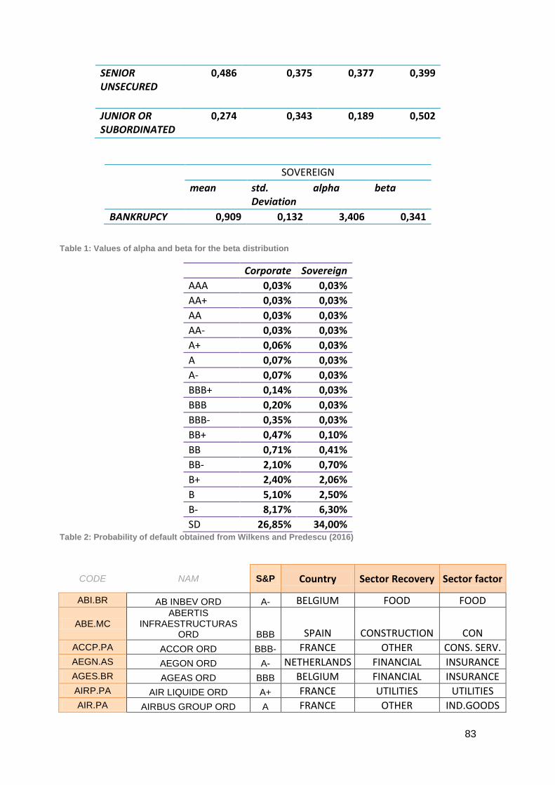
83
SENIOR UNSECURED
0,486 0,375 0,377 0,399
JUNIOR OR SUBORDINATED
0,274 0,343 0,189 0,502
SOVEREIGN
mean std. Deviation
alpha beta
BANKRUPCY 0,909 0,132 3,406 0,341
Table 1: Values of alpha and beta for the beta distribution
Corporate Sovereign
AAA 0,03% 0,03%
AA+ 0,03% 0,03%
AA 0,03% 0,03%
AA- 0,03% 0,03%
A+ 0,06% 0,03%
A 0,07% 0,03%
A- 0,07% 0,03%
BBB+ 0,14% 0,03%
BBB 0,20% 0,03%
BBB- 0,35% 0,03%
BB+ 0,47% 0,10%
BB 0,71% 0,41%
BB- 2,10% 0,70%
B+ 2,40% 2,06%
B 5,10% 2,50%
B- 8,17% 6,30%
SD 26,85% 34,00% Table 2: Probability of default obtained from Wilkens and Predescu (2016)
CODE NAM S&P Country Sector Recovery Sector factor
ABI.BR AB INBEV ORD A- BELGIUM FOOD FOOD
ABE.MC ABERTIS
INFRAESTRUCTURAS ORD BBB SPAIN CONSTRUCTION CON
ACCP.PA ACCOR ORD BBB- FRANCE OTHER CONS. SERV. AEGN.AS AEGON ORD A- NETHERLANDS FINANCIAL INSURANCE AGES.BR AGEAS ORD BBB BELGIUM FINANCIAL INSURANCE AIRP.PA AIR LIQUIDE ORD A+ FRANCE UTILITIES UTILITIES AIR.PA AIRBUS GROUP ORD A FRANCE OTHER IND.GOODS

84
CODE NAM S&P Country Sector Recovery Sector factor
ALVG.DE ALLIANZ ORD AA GERMANY FINANCIAL INSURANCE ACBr.AT ALPHA BANK R ORD SD GREECE FINANCIAL BANKS ALSO.PA ALSTOM ORD BBB- FRANCE TRANSPORT TRAVEL
AMA.MC AMADEUS IT HOLDING
ORD BBB SPAIN OTHER TECH
ISPA.AS ARCELORMITTAL ORD BB LUXEMBOURG STEEL
BASIC RESOURCE
AKE.PA ARKEMA ORD BBB FRANCE CHEMICAL CHEMICAL
ASMI.AS ASM INTL ORD BB+ NETHERLANDS FABRICATED PR.
BASIC RESOURCE
ATL.MI ATLANTIA ORD BBB+ ITALY CONSTRUCTION CON AXAF.PA AXA ORD A- FRANCE FINANCIAL INSURANCE
EMII.MI BANCA POPOLARE DELL EMILIA ROMA. ORD BB- ITALY FINANCIAL BANKS
BBVA.MC BANCO BILBAO VIZCAYA ARGENTARIA ORD BBB+ SPAIN FINANCIAL BANKS
BCP.LS BANCO COM ORD B+ PORTUGAL FINANCIAL BANKS
SABE.MC BANCO DE SABADELL ORD BB+ SPAIN FINANCIAL BANKS
POP.MC BANCO POPULAR ESPANOL ORD B+ SPAIN FINANCIAL BANKS
SAN.MC BANCO SANTANDER ORD A- SPAIN FINANCIAL BANKS BKIR.I BANK OF IRELAND ORD BBB- IRELAND FINANCIAL BANKS BKIA.MC BANKIA ORD BB+ SPAIN FINANCIAL BANKS BKT.MC BANKINTER ORD BBB- SPAIN FINANCIAL BANKS BASFn.DE BASF N ORD A GERMANY CHEMICAL CHEMICAL
BAYGn.DE BAYER N ORD A- GERMANY DRUGS
CONS. GOODS
GBFG.DE BILFINGER ORD BB+ GERMANY CONSTRUCTION CON BMWG.DE BMW ORD A+ GERMANY AUTOMOTIVE AUTO BNPP.PA BNP PARIBAS ORD A FRANCE FINANCIAL BANKS BOUY.PA BOUYGUES ORD BBB FRANCE CONSTRUCTION CON BNRGn.DE BRENNTAG N ORD BBB FRANCE CHEMICAL CHEMICAL CABK.MC CAIXABANK ORD BBB SPAIN FINANCIAL BANKS CAPP.PA CAP GEMINI ORD BBB FRANCE OTHER TECH CARR.PA CARREFOUR ORD BBB+ FRANCE RETAIL RETAIL
CASP.PA CASINO GUICHARD PERRACHON ORD BB+ FRANCE RETAIL RETAIL
CLNX.MC CELLNEX TELECOM ORD BB+ SPAIN OTHER TELECOM CNHI.MI CNH INDUSTRIAL ORD BB+ NETHERLANDS MACHINERY INDUSTRIALS COFB.BR COFINIMMO ORD BBB BELGIUM OTHER REAL STATE CBKG.DE COMMERZBANK ORD BBB+ GERMANY FINANCIAL BANKS
SGOB.PA COMPAGNIE DE SAINT GOBAIN ORD BBB FRANCE FABRICATED PR.
BASIC RESOURCE
CAGR.PA CREDIT AGRICOLE ORD A FRANCE FINANCIAL BANKS CRH.I CRH ORD BBB+ IRELAND FABRICATED PR. BASIC

85
CODE NAM S&P Country Sector Recovery Sector factor
RESOURCE
DAIGn.DE DAIMLER N ORD A- GERMANY AUTOMOTIVE AUTO DANO.PA DANONE ORD A- FRANCE FOOD FOOD DELB.BR DELHAIZE ORD BBB BELGIUM FOOD FOOD DBKGn.DE DEUTSCHE BANK N ORD BBB+ GERMANY FINANCIAL BANKS
DB1Gn.DE DEUTSCHE BOERSE N ORD AA GERMANY FINANCIAL FINANCIALS
LHAG.DE DEUTSCHE LUFTHANSA ORD BBB- GERMANY TRANSPORT TRAVEL
DTEGn.DE DEUTSCHE TELEKOM N ORD BBB+ GERMANY OTHER TELECOM
DWNG.DE DEUTSCHE WOHNEN ORD A- GERMANY OTHER REAL STATE
DIDA.MC DISTRIBUIDORA INTERN.DE ALIMEN. ORD BBB- SPAIN FOOD FOOD
EONGn.DE E.ON N ORD BBB+ GERMANY UTILITIES UTILITIES EDEN.PA EDENRED ORD BBB+ FRANCE FINANCIAL FINANCIALS EDF.PA EDF ORD A+ FRANCE UTILITIES UTILITIES ELI1V.HE ELISA ORD BBB+ FINLAND OTHER TECH ELE.MC ENDESA ORD BBB SPAIN UTILITIES UTILITIES ENEI.MI ENEL ORD BBB ITALY UTILITIES UTILITIES ENGIE.PA ENGIE ORD A FRANCE UTILITIES UTILITIES ENI.MI ENI ORD BBB+ ITALY OIL OIL
ERST.VI ERSTE GROUP BANK ORD BBB+ AUSTRIA FINANCIAL BANKS
EURBr.AT EUROBANK ERGASIAS/R ORD SD GREECE FINANCIAL BANKS
ETL.PA EUTELSAT COMMUNICATIONS ORD BBB FRANCE FABRICATED PR. TELECOM
EVKn.DE EVONIK INDUSTRIES ORD BBB+ GERMANY CHEMICAL CHEMICAL
EXOR.MI EXOR ORD BBB+ ITALY FINANCIAL FINANCIALS FER.MC FERROVIAL ORD BBB SPAIN CONSTRUCTION CON
FCHA.MI FIAT CHRYSLER AUTOMOBILES ORD BB ITALY AUTOMOTIVE AUTO
SIFI.MI FINMECCANICA ORD BB+ ITALY OTHER TECH
FDR.PA FONCIERE DES REGIONS REIT BBB FRANCE FINANCIAL FINANCIALS
FUM1V.HE FORTUM ORD BBB+ FINLAND UTILITIES UTILITIES
FMEG.DE FRESENIUS MEDICAL CARE ORD BBB- GERMANY OTHER
HEALTH CARE
FREG.DE FRESENIUS ORD BBB- GERMANY OTHER
HEALTH CARE
GAS.MC GAS NATURAL ORD BBB SPAIN UTILITIES UTILITIES GFCP.PA GECINA REIT BBB+ FRANCE OTHER IND.GOODS
GRLS.MC GRIFOLS ORD CL A BB SPAIN OTHER
HEALTH CARE
HNRGn.DE HANNOVER RUCKVERSICHERUNG N AA- GERMANY FINANCIAL INSURANCE
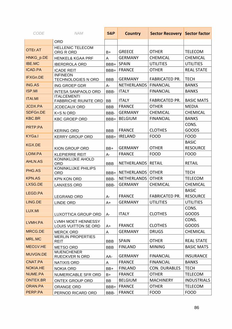
86
CODE NAM S&P Country Sector Recovery Sector factor
ORD
OTEr.AT HELLENIC TELECOM ORG R ORD B+ GREECE OTHER TELECOM
HNKG_p.DE HENKEL& KGAA PRF A GERMANY CHEMICAL CHEMICAL IBE.MC IBERDROLA ORD BBB+ SPAIN UTILITIES UTILITIES ICAD.PA ICADE REIT BBB+ FRANCE OTHER REAL STATE
IFXGn.DE INFINEON TECHNOLOGIES N ORD BBB GERMANY FABRICATED PR. TECH
ING.AS ING GROEP GDR A- NETHERLANDS FINANCIAL BANKS ISP.MI INTESA SANPAOLO ORD BBB- ITALY FINANCIAL BANKS
ITAI.MI ITALCEMENTI FABBRICHE RIUNITE ORD BB ITALY FABRICATED PR. BASIC MATS
JCDX.PA JCDECAUX ORD BBB FRANCE OTHER MEDIA SDFGn.DE K+S N ORD BBB- GERMANY CHEMICAL CHEMICAL KBC.BR KBC GROEP ORD BBB+ BELGIUM FINANCIAL BANKS
PRTP.PA KERING ORD BBB FRANCE CLOTHES
CONS. GOODS
KYGa.I KERRY GROUP ORD BBB+ IRELAND FOOD FOOD
KGX.DE KION GROUP ORD BB+ GERMANY OTHER
BASIC RESOURCE
LOIM.PA KLEPIERRE REIT A- FRANCE FOOD FOOD
AHLN.AS KONINKLIJKE AHOLD ORD BBB NETHERLANDS RETAIL RETAIL
PHG.AS KONINKLIJKE PHILIPS ORD BBB+ NETHERLANDS OTHER TECH
KPN.AS KPN KON ORD BBB- NETHERLANDS OTHER TELECOM LXSG.DE LANXESS ORD BBB- GERMANY CHEMICAL CHEMICAL
LEGD.PA LEGRAND ORD A- FRANCE FABRICATED PR.
BASIC RESOURCE
LING.DE LINDE ORD A+ GERMANY UTILITIES UTILITIES
LUX.MI LUXOTTICA GROUP ORD A- ITALY CLOTHES
CONS. GOODS
LVMH.PA LVMH MOET HENNESSY LOUIS VUITTON SE ORD A+ FRANCE CLOTHES
CONS. GOODS
MRCG.DE MERCK ORD A GERMANY DRUGS CHEMICAL
MRL.MC MERLIN PROPERTIES REIT BBB SPAIN OTHER REAL STATE
MEO1V.HE METSO ORD BBB FINLAND MINING BASIC MATS
MUVGN.DE MUENCHENER RUECKVER N ORD AA- GERMANY FINANCIAL INSURANCE
CNAT.PA NATIXIS ORD A FRANCE FINANCIAL BANKS NOKIA.HE NOKIA ORD BB+ FINLAND CON. DURABLES TECH NUME.PA NUMERICABLE SFR ORD B+ FRANCE OTHER TELECOM ONTEX.BR ONTEX GROUP ORD BB BELGIUM MACHINERY INDUSTRIALS ORAN.PA ORANGE ORD BBB+ FRANCE OTHER TELECOM PERP.PA PERNOD RICARD ORD BBB- FRANCE FOOD FOOD

87
CODE NAM S&P Country Sector Recovery Sector factor
PST.MI POSTE ITALIANE ORD BBB- ITALY OTHER CONS. SERV. PTNL.AS POSTNL ORD BBB- NETHERLANDS RETAIL RETAIL PROX.BR PROXIMUS ORD A BELGIUM OTHER TELECOM PUBP.PA PUBLICIS GROUPE ORD BBB+ FRANCE OTHER MEDIA
RBIV.VI RAIFFEISEN BANK INTERNATIONAL ORD BBB AUSTRIA FINANCIAL BANKS
REE.MC RED ELECTRICA CORPORACION ORD A- SPAIN UTILITIES UTILITIES
RENA.PA RENAULT PAR BBB- FRANCE AUTOMOTIVE AUTO REP.MC REPSOL ORD BBB- SPAIN OIL OIL
RXL.PA REXEL ORD BB FRANCE FABRICATED PR.
BASIC RESOURCE
RRTL.DE RTL GROUP ORD BBB+ GERMANY OTHER MEDIA RWEG.DE RWE ORD BBB GERMANY UTILITIES UTILITIES RYA.I RYANAIR HOLDINGS ORD BBB+ IRELAND TRANSPORT TRAVEL SAMAS.HE SAMPO A ORD A- FINLAND FINANCIAL FINANCIALS
SASY.PA SANOFI ORD AA FRANCE OTHER
HEALTH CARE
SAPG.DE SAP ORD A GERMANY OTHER TECH
SCHN.PA SCHNEIDER ELECTRIC SE ORD A- FRANCE UTILITIES TECH
SCOR.PA SCOR ORD AA- FRANCE FINANCIAL INSURANCE SESFd.PA SES FDR BBB LUXEMBOURG OTHER TELECOM
SIEGN.DE SIEMENS N ORD A+ GERMANY CON. DURABLES
CONS. GOODS
SKG.I SMURFIT KAPPA GROUP ORD BB+ IRELAND FABRICATED PR.
BASIC RESOURCE
SRG.MI SNAM ORD BBB ITALY OIL OIL
SOGN.PA SOCIETE GENERALE ORD A FRANCE FINANCIAL BANKS
EXHO.PA SODEXO ORD A- GERMANY OTHER CONS. SERV. SOLB.BR SOLVAY ORD BBB- BELGIUM CHEMICAL CHEMICAL
STM.PA STMICROELECTRONICS ORD BBB- FRANCE OTHER TECH
STERV.HE STORA ENSO R ORD BB FINLAND FABRICATED PR.
BASIC RESOURCE
TCH.PA TECHNICOLOR ORD B+ FRANCE OTHER MEDIA TECF.PA TECHNIP ORD BBB+ FRANCE CONSTRUCTION CON TLIT.MI TELECOM ITALIA ORD BB+ ITALY OTHER TELECOM TEF.MC TELEFONICA ORD BBB SPAIN OTHER TELECOM
TNET.BR TELENET GROUP HOLDING ORD B+ BELGIUM OTHER TELECOM
TRN.MI TERNA RETE ELETTRICA NAZIONALE ORD BBB ITALY UTILITIES UTILITIES
TKAG.DE THYSSENKRUPP ORD BB GERMANY STEEL BASIC MATS TNTE.AS TNT EXPRESS ORD BBB NETHERLANDS RETAIL RETAIL

88
CODE NAM S&P Country Sector Recovery Sector factor
TOTF.PA TOTAL ORD A+ FRANCE UTILITIES UTILITIES UNBP.AS UNIBAIL RODAMCO REIT A FRANCE FINANCIAL FINANCIALS CRDI.MI UNICREDIT ORD BBB- ITALY FINANCIAL BANKS ULVR.L UNILEVER ORD A+ LUXEMBOURG CHEMICAL CHEMICAL
UBI.MI UNIONE DI BANCHE ITALIANE ORD BBB- ITALY FINANCIAL BANKS
UPM1V.HE UPM KYMMENE ORD BB+ FINLAND FABRICATED PR.
BASIC RESOURCE
VLOF.PA VALEO ORD BBB FRANCE AUTOMOTIVE AUTO
VIE.PA VEOLIA ENVIRONNEMENT VE ORD BBB FRANCE UTILITIES UTILITIES
VIV.PA VIVENDI ORD BBB FRANCE OTHER MEDIA VOWG_p.DE VOLKSWAGEN NV PRF BBB+ GERMANY AUTOMOTIVE AUTO VNAn.DE VONOVIA ORD BBB+ GERMANY OTHER REAL STATE MWDP.PA WENDEL ORD BBB- FRANCE FINANCIAL FINANCIALS
WLSNc.AS WOLTERS KLUWER C ORD BBB+ NETHERLANDS OTHER TECH
95740@orgid AUSTRIA AA+ 95744@orgid BELGIUM AA 95765@orgid FINLAND AA+ 95766@orgid FRANCE AA 96805@orgid GERMANY AAA 95769@orgid GREECE B- 69201@orgid IRELAND A+ 95779@orgid ITALY BBB- 95794@orgid NETHERLANDS AAA 95804@orgid PORTUGAL BB+ 162600@orgid SPAIN BBB+ Table 3: Assets employed in the empirical exercise
Note for the tables 4, 5, 6,7, 8, 9, 10, 11 and 12:
The composition of each portfolio is the following:
1. Corporate debt
1.1 Second factor: country
1.2 Second factor: industry
2. Equity
2.1 Second factor: country
2.2 Second factor: industry
3 Sovereign debt
4 Corporate and sovereign debt
5 Debt and equity
The criteria for building the portfolios are the following: A. Equally-weighted
B. Minimum variance
C. Minimum variance (allowing only long positions)
D. Lower default correlation weighted by rating
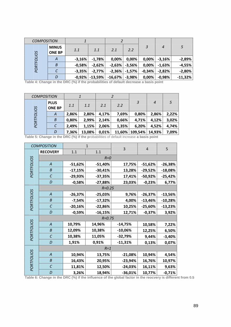
89
COMPOSITION 1 2
3 4 5
PO
RTF
OLI
OS
MINUS ONE BP
1.1 1.1 2.1 2.2
A -3,16% -1,78% 0,00% 0,00% 0,00% -3,16% -2,89%
B -0,58% -2,62% -2,63% -3,56% 0,00% -1,63% -4,55%
C -3,35% -2,77% -2,36% -1,57% -0,34% -2,82% -2,80%
D -0,92% -13,59% -16,67% -3,98% 0,00% -0,98% -11,32% Table 4: Change in the DRC (%) if the probabilities of default decrease a basis point
COMPOSITION 1 2
3 4 5
PO
RTF
OLI
OS
PLUS ONE BP
1.1 1.1 2.1 2.2
A 2,86% 2,80% 4,17% 7,69% 0,80% 2,86% 2,22%
B 0,80% 2,99% 2,14% 0,66% 4,71% 4,12% 3,02%
C 2,49% 1,15% 2,06% 1,35% 6,20% 4,52% 4,74%
D 7,36% 13,08% 0,01% 11,60% 109,54% 14,93% 7,09% Table 5: Change in the DRC (%) if the probabilities of default increase a basis point
COMPOSITION 1 3 4 5
PO
RTF
OLI
OS
RECOVERY 1.1 1.1
R=0
A -51,62% -51,40% 17,75% -51,62% -26,38%
B -17,15% -30,41% 13,28% -29,52% -18,08%
C -29,93% -37,35% 17,41% -50,92% -25,42%
D -0,58% -27,88% 23,03% -0,23% 6,77%
PO
RTF
OLI
OS R=0.25
A -26,37% -25,03% 9,76% -26,37% -13,56%
B -7,54% -17,32% 4,00% -13,46% -10,28%
C -20,16% -22,86% 10,25% -25,60% -13,23%
D -0,59% -16,15% 12,71% -0,37% 3,92%
PO
RTF
OLI
OS R=0.75
A 10,79% 14,96% -14,75% 10,58% 7,22%
B 12,09% 10,38% -10,06% 12,25% 6,50%
C 10,38% 11,05% -32,79% 9,44% -3,40%
D 1,91% 0,91% -11,31% 0,13% 0,07%
PO
RTF
OLI
OS R=1
A 10,94% 13,75% -21,08% 10,94% 4,54%
B 16,43% 20,95% -23,94% 16,76% 10,97%
C 11,81% 12,50% -24,03% 16,11% 9,63%
D 3,26% 18,94% -36,01% 10,77% -0,71% Table 6: Change in the DRC (%) if the influence of the global factor in the reocvery is different from 0.5

90
COMPOSITION 1 2
3 4 5 P
OR
TFO
LIO
S
OLS 1.1 1.1 2.1 2.2
A 4,37% 0,74% 7,69% 7,69% 0,43% 4,37% 5,25%
B 19,51% -1,49% 9,88% 1,50% -8,41% 4,65% 0,05%
C 15,56% -8,47% 10,93% -2,58% -9,38% 4,96% 5,71%
D -6,66% 15,44% -9,99% -11,20%
-47,07% -2,61% -5,87%
Table 7 : Change in the DRC (%) if the OLS values of the parameters are employed
COMPOSITION 1 2
3 4 5
PO
RTF
OLI
OS QUARTERLY 1.1 1.1 2.1 2.2
A -2,82% 9,81% 7,69% 15,38% -0,55% -2,82% -3,20%
B 50,36% 0,46% 38,33% 19,88% 10,04% -25,38% -27,86%
C 0,74% 134,48% 170,98% 149,84% -23,15% -26,83% -27,31%
D 23,16% 10,80% -18,66% -5,53% 47,16% 50,49% -9,41% Table 8: Change in the DRC (%) if the quarterly data is employed
COMPOSITION 1 2
3 4 5
PO
RTF
OLI
OS COPULA 1.1 1.1 2.1 2.2
A 90,66% 115,35% 84,62% 100,00% 12,37% 90,13% 94,33%
B 32,93% 29,84% 19,46% 22,84% 15,42% 14,16% 11,36%
C 77,64% 110,24% 74,03% 103,42% 10,90% 80,70% 82,57%
D 18,67% 65,68% 20,56% 36,02% 10,79% 14,74% 21,23% Table 9: Change in the DRC (%) a Clayton copula is employed in the systematic factors
COMPOSITION 1 2 3 4 5
NOMINAL:100 € INITIAL VALUES
1.1 1.1 2.1 2.2
PO
RTF
OLI
OS A 6,93 7,33 7,69 8,33 4,23 3,47 4,91
B 17,32 21,35 22,53 26,18 1,08 11,20 11,89
C 5,80 6,59 6,94 7,45 0,88 3,56 3,77
D 4,08 5,95 10,01 8,97 0,35 2,74 4,90
Table 10: Initial DRC values for the portfolios
NOMINAL: a
million PLAIN MONTECARLO
MEAN
1 2
3 4 5 1.1 1.2 2.1 2.2
A 50962,04 49511,23 51282,05 76923,08 41216,28 25490,16 34114,53
B 126884,10 127461,09 215169,39 226470,14 10534,85 79882,33 84544,99

91
C 78957,68 73913,37 113993,83 114783,19 8821,83 17949,19 18977,46
D 54231,82 60578,99 101628,08 109204,99 3072,96 39709,63 44698,81
NOMINAL: a million ANTITHETIC VARIANTES MONTECARLO
MEAN
1 2
3 4 5 1.1 1.2 2.1 2.2
A 50949,19 49426,59 51282,05 76923,08 41411,62 25482,86 34110,03
B 126960,41 127432,89 215413,28 225607,79 10526,81 79680,21 84611,88
C 79285,22 73847,23 113993,83 115267,20 8821,16 17769,19 18821,23
D 54159,96 59847,17 101464,46 109536,86 2980,06 39563,45 44617,75
Table 11: Mean of the values of VaR using plain MC and antithetic MC
NOMINAL: a million PLAIN MONTECARLO
VARIANCE 1 2
3 4 5 1.1 1.2 2.1 2.2
A 84513,042 1187980,04 8,56E-22 3,42E-21 1199024,32 20412,3564 6175,05319
B 12013816,8 7672854,81 199724509 13596419,1 178007,626 5386021,86 2406490,54
C 10676049,6 12553324 7,70E-21 4639290,23 143187,452 762502,147 676632,747
D 3583995,1 9301576,25 5876518,24 122563954 1174558,98 4882379,49 6740081,31
NOMINAL: a million ANTITHETIC VARIANTES MONTECARLO
VARIANCE 1 2
3 4 5 1.1 1.2 2.1 2.2
A 40383,6889 585852,419 8,5559E-22 3,4224E-21 578669,339 9718,58452 2930,06151
B 5428711,07 3304426,89 113109304 17811248,9 87209,7088 3126272,79 1390247,68
C 2989810,52 9282759,93 7,7003E-21 3411591,68 71736,6875 411034,659 380788,867
D 2196621,33 4784478,21 1773391,37 56080330,2 685460,003 2495714,88 3662342,24 Table 12: Variance of the values of VaR using plain MC and antithetic MC

92
8.2. Appendix of figures
Gaussian copula
Clayton copula
idyosincratic component
Normal
factor 1 factor 2 Normal Normal
Figure 1: Structure of a two-level nested copulas with normal marginal distribution
Figure 2: DECO correlation from 1995-2005 across the main stock market indexes.
Note: the indexes employed for this goal are the followings: AEX index for Netherlands, BEL20 for Belgium,
DAX30 for Germany, CAC40 for France, IBEX35 for Spain, ATX for Austria, ISEQ for Ireland and PSI20 for
Portugal.
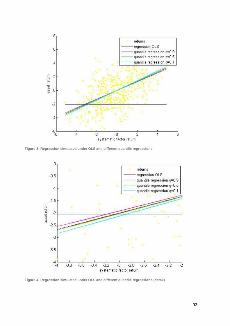
93
Figure 3: Regression simulated under OLS and different quantile regressions
Figure 4: Regression simulated under OLS and different quantile regressions (detail)

94
Figure 5: Residuals and weight for the residual under each different regression employed Note that the values of the optimization function have been scaled in order to compare sensibly.

95
Figure 6: Country of the equity from Eurostoxx employed in the sensitivity analysis

96
Figure 7: Rating of the equity from Eurostoxx employed in the sensitivity analysis
Figure 8: Sector of the equity from Eurostoxx employed in the sensitivity analysis
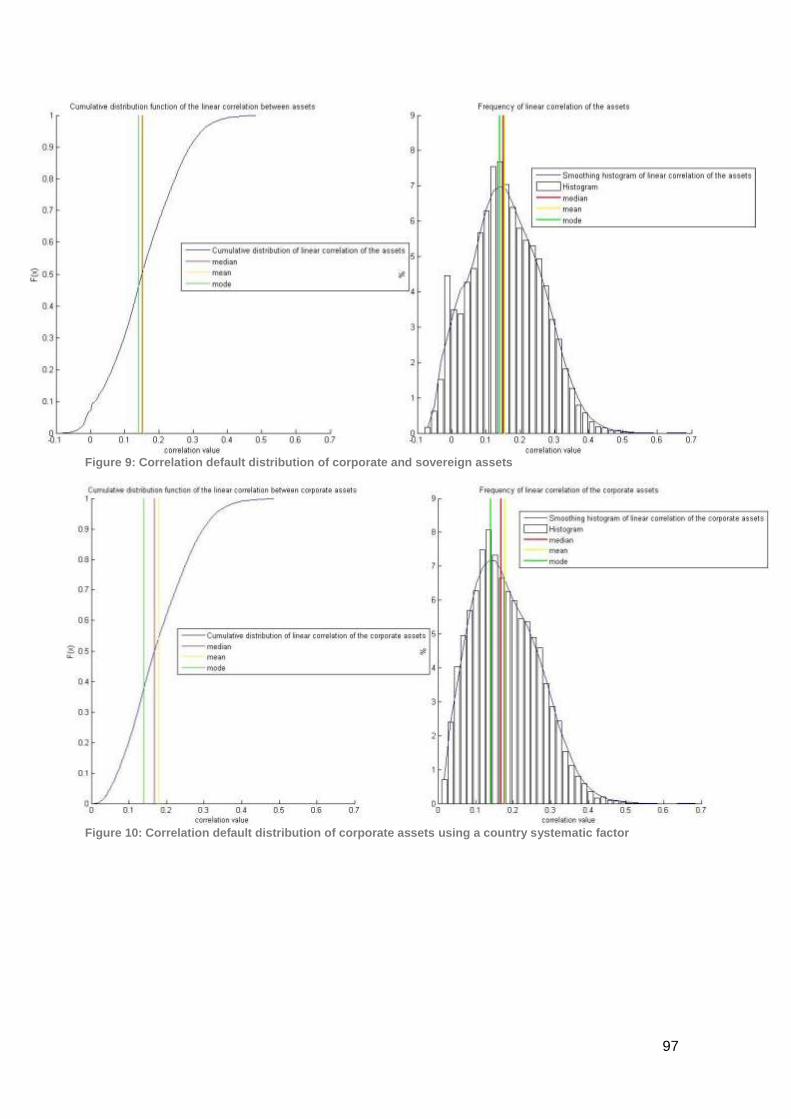
97
Figure 9: Correlation default distribution of corporate and sovereign assets
Figure 10: Correlation default distribution of corporate assets using a country systematic factor

98
Figure 11: Correlation default distribution of corporate assets using a industry systematic factor
Figure 12: Number of defaults depending on the chosen second systematic factor

99
Figure 13: LGD for NUMERICABLE SFR using different values for the parameter of influence of the global factor in equation (19)
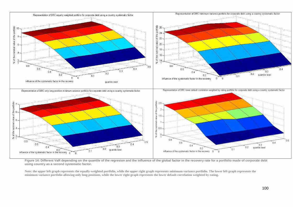
100
Figure 14: Different VaR depending on the quantile of the regresion and the influence of the global factor in the recovery rate for a portfolio made of corporate debt using country as a second systematic factor.
Note: the upper left graph represents the equally-weighted portfolio, while the upper right graph represents minimum variance portfolio. The lower left graph represents the
minimum variance portfolio allowing only long positions, while the lower right graph represents the lower default correlation weighted by rating.

101
Figure 15: Different VaR depending on the quantile of the regresion and the influence of the global factor in the recovery rate for a portfolio made of corporate debt using industry as a second systematic factor.
Note: the upper left graph represents a portfolio made of corporate debt using country as a second systematic factor, while the upper right graph represents the same portfolio using
industry as a second systematic factor. The lower left graph represents a sovereign debt portfolio, while the lower right graph represents a portfolio of corporate and sovereign debt.

102
Figure 16: Estimated parameters test (q=0.2 regression against OLS regression) for BBVA returns using country (upper)or sector (lower) as a second factor

103
Figure 17:Estimated parameters test (monthly against quarterly data employed to a q=0.2 quantile regression) for BBVA returns using country (upper)or sector (lower)as a second factor

104
Figure 18: DRC of the different portfolios and the increase if a Clayton copula is employed in the systematic factors
0
2
4
6
8
10
12
14
16
18
1.1 1.2 2.1 2.2 3 4 5
%
DRC PORTFOLIO A
DRC Δ con cópulas
0
5
10
15
20
25
30
35
1.1 1.2 2.1 2.2 3 4 5
%
DRC PORTFOLIO B
DRC Δ con cópulas
0
2
4
6
8
10
12
14
16
1.1 1.2 2.1 2.2 3 4 5
%
DRC PORTFOLIO C
DRC Δ con cópulas
0
2
4
6
8
10
12
14
1.1 1.2 2.1 2.2 3 4 5
%
DRC PORTFOLIO D
DRC Δ con cópulas