Embed Size (px)
Citation preview
Modelling and simulation of the dynamic behaviour of
the automobile
Raffaele Di Martino
To cite this version:
Raffaele Di Martino. Modelling and simulation of the dynamic behaviour of the automobile.Automatic. Universite de Haute Alsace - Mulhouse, 2005. English.
HAL Id: tel-00736040
https://tel.archives-ouvertes.fr/tel-00736040
Submitted on 27 Sep 2012
HAL is a multi-disciplinary open accessarchive for the deposit and dissemination of sci-entific research documents, whether they are pub-lished or not. The documents may come fromteaching and research institutions in France orabroad, or from public or private research centers.
L’archive ouverte pluridisciplinaire HAL, estdestinee au depot et a la diffusion de documentsscientifiques de niveau recherche, publies ou non,emanant des etablissements d’enseignement et derecherche francais ou etrangers, des laboratoirespublics ou prives.

FACULTY OF ENGINEERING
Course of degree in Mechanical Engineering
Thesis of degree
Modelling and Simulation of the Dynamic Behaviour of
the Automobile
Author: Supervisor:
Di Martino Raffaele Professor Gérard Léon Gissinger
Matr. 165/000101
Co-Supervisor:
Professor Gianfranco Rizzo
Dr. Eng. Ivan Arsie
Università degli Studi di Salerno
UHA Université de Haute Alsace

Academic year 2004/2005
Title of degree
Modelling and Simulation of the Dynamic Behaviour of
the Automobile
by
Di Martino Raffaele
Thesis submitted to the Faculty of Engineering,
University of Salerno
in partial fulfilment of the requirements for the degree of
DOCTOR IN MECHANICAL ENGINEERING
Author: Supervisor:
Di Martino Raffaele Professor G. L. Gissinger
Matr. 165/000101 Co-Supervisor:
Professor G. Rizzo
Dr. Eng. Ivan Arsie

_________________________________________________________________________________ i
Modelling and Simulation of the Dynamic Behaviour
of the Automobile
Raffaele Di Martino
G. L. Gissinger Supervisor and G. Rizzo Co-Supervisor
Mechanical Engineering Abstract This study, carried out in cooperation with ESSAIM, Ecole Supérieure des Sciences
Appliquées pour l’Ingénieur, Mulhouse in France, was aimed at developing accurate
mathematical models of some types of tyre, in order to analyze their influence on
vehicle dynamics. The complete vehicle was studied under dynamic conditions, to
quantify the influence of all factors, such as rolling forces, aerodynamic forces and
many others, acting on their components on torque distribution and vehicle dynamics.
Mathematical models for two common types of vehicle, namely front and rear wheel
drive, each ones equipped with the different types of tyre, were developed. Both models
were used to simulate the behaviour of a real vehicle, developing complete simulation
software, developed in Matlab-Simulink environment at MIPS, Modélisation
Intelligence Processus Systèmes. Therefore, this car model, running on a straight and
curve track, was also developed, to get a qualitative insight of the influence of these
kinds of interactions on traction capabilities. The software, used to simulate some
dynamics manoeuvres, shows up the basic behaviour of vehicle dynamics.
_________________________________________________________________________________ ii
Dedication Dedicated to my grandmother, who, with her love, patience, and encouragement
during my studies, made this aim possible.

_________________________________________________________________________________ iii
Acknowledgements I would like to express my gratitude to some of the people who contributed to this work.
First, I would like to thank my Professor G. Rizzo for his guidance and direction in the
development and conduct of this research. I would like to thank Professor G.L.
Gissinger, my advisor for the duration, for supporting me during my time here at
ESSAIM, Ecole Supérieure des Sciences Appliquées pour l’Ingénieur, Mulhouse in
France. During these six months they have also been friendly and I sincerely hope we
find opportunities in the future to work together once again. Conteins
Professor Michel Basset and Assistant Professor Jean Philippe Lauffenburger must also
be mentioned for their insightful comments that have exemplified the work during the
development of my thesis.
I would also like to extend my thank to Doctor Engineer Ivan Arsie and Professor
Cesare Pianese for their encouragement and invaluable assistance.
Anyone who was around when I began my work knows that I have to express my
gratitude to Engineer Eduardo Haro Sandoval, for his patience, expertise, and support
during my six moths in the Research Laboratory. Many thanks must be given to Ing.
Julien Caroux, for his assistance in developing and programming the software dedicated
to study about the behaviour of the vehicle. Both, friendship have made the last six
months very enjoyable.
Above anyone else I would like to thank, Engineer Alfonso Di Domenico and Engineer
Michele Maria Marotta, who, trough their assistance have made some moments could
be overcome easily.
Lastly, I would like to thank my parents, and other people close to me for giving me the
opportunity to come to the University of Haute-Alsace. They have been a tremendous
emotional and psychological support to me throughout these few months and for that I
am eternally thankful. I sincerely believe that this work would not exist without their
guidance and support.

_________________________________________________________________________________ iv
Table of Contents Abstract............................................................................................................................. i Dedication ........................................................................................................................ ii Acknowledgements ........................................................................................................iii Table of Contents ........................................................................................................... iv List of Figures................................................................................................................. vi List of Tables ................................................................................................................... x List of Symbols ............................................................................................................... xi 1 Introduction.................................................................................................................. 1
1.1 Historical Notes on Vehicles ............................................................................. 1 1.2 Thesis Outline .................................................................................................... 5
2 Vehicle Dynamics......................................................................................................... 7 2.1 Motivation for Studying Vehicle Dynamics ...................................................... 7 2.2 Motivation for this Research.............................................................................. 9
2.2.1 Research Objective ................................................................................. 10 2.2.2 Literature Review ................................................................................... 10
3 Vehicle Dynamics Modelling..................................................................................... 15 3.1 Axis System ..................................................................................................... 15
3.1.1 Earth-Fixed Axis System........................................................................ 16 3.1.2 Vehicle Axis System............................................................................... 16
3.2 Mechanism of Pneumatic Tyres ...................................................................... 18 3.2.1 Force Acting Between Road and Wheel................................................. 18 3.2.2 Constitutive Equations............................................................................ 31
4 Longitudinal Dynamics Model ................................................................................. 38 4.1 Physical Model ................................................................................................ 38 4.2 Powertrain Modelling ...................................................................................... 40
4.2.1 Engine Model: Characteristics of Internal Combustion Engines............ 41 4.2.2 Gear Box and Torque Converter............................................................. 44
4.3 Driver Model.................................................................................................... 44 4.4 Equivalent Dynamic System............................................................................ 44
4.4.1 Reduction of Forces Acting on the Vehicle............................................ 49 4.4.2 Reduction of Inertias of the Vehicle ....................................................... 54
4.5 Simulation for longitudinal Model with Gearbox............................................ 67 4.5.1 Method of Vehicle-Simulation ............................................................... 67 4.5.2 Simulation Results .................................................................................. 68
5 Lateral Dynamics Model ........................................................................................... 75 5.1 Working Hypotheses........................................................................................ 75 5.2 Theoretical Model............................................................................................ 76
5.2.1 Equations of Congruence........................................................................ 78 5.2.2 Equations of Equilibrium........................................................................ 84 5.2.3 Constitutive Equations............................................................................ 88
5.3 Single-Track Model ......................................................................................... 89 5.4 Two/Four-Degree-of-Freedom Vehicle Model Derivation ............................. 89

List of Contens________________________________________________________________________
_________________________________________________________________________________ v
5.5 Equations of Motion ........................................................................................ 90 5.5.1 Rear Traction Model (RWD).................................................................. 91 5.5.2 Front Traction Model (FWD) ............................................................... 106 5.5.3 Conclusions........................................................................................... 111
6 Simulink Environment Model ................................................................................ 113 6.1 Simulink Modelling ....................................................................................... 113 6.2 Simulating a Complete Vehicle ..................................................................... 114
6.2.1 Driver Behaviour .................................................................................. 115 6.2.2 Powertrain Modelling ........................................................................... 116 6.2.3 Vehicle Dynamics................................................................................. 122 6.2.4 Tyre Model ........................................................................................... 128 6.2.5 Real time Simulator Block.................................................................... 132
7 Validation of the Vehicle Model ............................................................................. 135 7.1 The Simulation of the Systems ...................................................................... 135 7.2 Validation Procedure ..................................................................................... 136
7.2.1 Definition of a Test Protocol ................................................................ 136 7.2.2 Data Acquisition. Measures.................................................................. 137 7.2.3 Elements of the Measure Chain ............................................................ 138 7.2.4 Tests and Measurements....................................................................... 139 7.2.5 Instrumentation of Vehicle ................................................................... 139 7.2.6 Definition of Tests ................................................................................ 141 7.2.7 Circuit Test ........................................................................................... 141 7.2.8 Handling of Data................................................................................... 142 7.2.9 Analysis of the Results ......................................................................... 144
8 Conclusions and Recommendations for Future Research ................................... 157 8.1 Conclusion ..................................................................................................... 157
8.1.1 Practical Use ......................................................................................... 158 8.1.2 Improvement on Overall Approach ...................................................... 158
8.2 Future Research ............................................................................................. 159 8.2.1 Optimal Control Methods ..................................................................... 159 8.2.2 Parallel Processing Computation .......................................................... 160 8.2.3 Using Different Vehicle and Tyre Models ........................................... 160
Appendix A.................................................................................................................. 162 Appendix B .................................................................................................................. 164 Appendix C.................................................................................................................. 166 References.................................................................................................................... 169

_________________________________________________________________________________ vi
List of Figures Figure 1.1:One-Wheel Vehicle (Rousseau-Workshops, France,wheel radius 2 m, without steer, 1869) .......................................................................................................... 2 Figure 1.2: Two-Wheel Vehicle (Turri and Porro, Italia, 1875)....................................... 2 Figure 1.3: Production Three-Wheel Vehicle (1929 Morgan Super Sports Aero) ........... 3 Figure 1.4: Production Four-Wheel Vehicle (1963 Austin Healey 3000 MKII).............. 4 Figure 1.5: Multiple-Wheel Ground Vehicle: The Train.................................................. 5 Figure 2.1: Literature Review Keyword Search Diagram. ............................................. 11 Figure 2.2: The Driver-Vehicle-Ground System [22]. ................................................... 13 Figure 2.3: Basic Structure of Vehicle System Dynamics.............................................. 14 Figure 3.1: Axis Systems after Guiggiani [20] ............................................................... 16 Figure 3.2: Sideslip Angle after Guiggiani [20]. ............................................................ 17 Figure 3.3: Walking Analogy to Tyre Slip Angle after Milliken [18]............................ 18 Figure 3.4: SAE Tyre Axis System after Gillespie [19]. ................................................ 19 Figure 3.5: Geometrical Configuration and Peripheral Speed in the Contact Zone. ...... 20 Figure 3.6: (a)Wheel Deformation in owing to Rolling Resistent (Ground Deformation and Elastic Return); (b) Forces and Contact Pressure σz in a Rolling Wheel. ................ 23 Figure 3.7 Generalized Forces Acting on the Vehicle.................................................... 26 Figure 3.8: Generalized Forces Acting on the Vehicle................................................... 29 Figure 3.9: Lateral Force versus Slip Angle. .................................................................. 32 Figure 3.10: Lateral Force versus Wheel Rounds in Transient Condition with Permanent Value equal to 2.4 kN. .................................................................................................... 35 Figure 3.11: Front Lateral Force versus Slip Angle with Different Normal Load. ........ 37 Figure 3.12: Rear Lateral Force versus Slip Angle with Different Normal Load. ......... 37 Figure 4.1: Primary Elements in the Powertrain............................................................. 39 Figure 4.2: Schematization Elements in the Powertrain................................................. 39 Figure 4.3: Powertrain Components and Configurations Theoretical Model................. 40 Figure 4.4: Performance Characteristic of Test-Vehicle ................................................ 43 Figure 4.5: Dimensionless Performance Characteristic of Test-Vehicle........................ 43 Figure 4.6: Driveline Notations ...................................................................................... 45 Figure 4.7: Driveline Complex Model. (a) Transmission Engaged; (b) Transmission Disengaged...................................................................................................................... 46 Figure 4.8: Equivalent System for a Driveline Model.................................................... 46 Figure 4.9: Description of Correcting Rod of Internal Combustion Engine. ................. 57 Figure 4.10: Maximum Acceleration as function of the Speed. ..................................... 60 Figure 4.11: Maximum Acceleration as function of the Speed in log scale and reverse......................................................................................................................................... 60 Figure 4.12: Function 1/a(u) and Search for the Optimum Speeds for Gear Shifting.... 61 Figure 4.13: Function 1/a(u) and Search for the Optimum Speeds for Gear Shifting; the white area is the time to speed. ....................................................................................... 61 Figure 4.14: Function 1/ax(u) in log scale. ..................................................................... 62 Figure 4.15: Engine Speed versus Vehicle Speed. ......................................................... 62 Figure 4.16: Acceleration-time curve. ........................................................................... 63

List of Figures________________________________________________________________________
_________________________________________________________________________________ vii
Figure 4.17: Speed-time curve........................................................................................ 63 Figure 4.18: Distance-time curve................................................................................... 64 Figure 4.19: Traction tyre curve. ................................................................................... 64 Figure 4.20: Traction Control curve. .............................................................................. 65 Figure 4.21: : Power-time curve. .................................................................................... 65 Figure 4.22: Torque-time curve. ..................................................................................... 66 Figure 4.23: Power versus Engine Velocity. .................................................................. 66 Figure 4.24: Torque versus Engine Velocity. ................................................................. 67 Figure 4.25: Throttle Opening Input............................................................................... 68 Figure 4.26: Test Vehicle, Renault Mégane Coupé 16V 150 HP................................... 69 Figure 4.27: Acceleration-time curve. ............................................................................ 70 Figure 4.28: Velocity-time curve.................................................................................... 71 Figure 4.29: Displacement-time curve............................................................................ 71 Figure 4.30: Traction Control curve. .............................................................................. 72 Figure 4.31: Power-time curve. ...................................................................................... 72 Figure 4.32: Torque-time curve. ..................................................................................... 73 Figure 4.33: Reference Acceleration and Velocity of the Vehicle [25] ......................... 73 Figure 4.34: Reference Normal and Tangential Forces at Rear Tyre [25] ..................... 74 Figure 4.35: Reference Powers Transferred [25]............................................................ 74 Figure 5.1: Vehicle Model. ............................................................................................. 76 Figure 5.2: Kinematics Steering (slip angle null) ........................................................... 77 Figure 5.3: Definition of kinematics Quantities of the Vehicle...................................... 79 Figure 5.4: Lateral Components of Velocity at Front Tyres........................................... 80 Figure 5.5: Lateral Components of Velocity at Rear Tyres............................................ 80 Figure 5.6: Longitudinal Components of Velocity at Left Tyres. .................................. 81 Figure 5.7: Longitudinal Components of Velocity at Right Tyres ................................. 82 Figure 5.8: Relation between Slip Angles and Centre of Rotation Position................... 82 Figure 5.9: Trajectory of the Vehicle as regards to a Reference Coordinate System..... 85 Figure 5.10: Forces Acting on the Vehicle ..................................................................... 88 Figure 5.11: Reduction of Single Track Model. ............................................................ 90 Figure 5.12: Single Track Model.................................................................................... 92 Figure 5.13: Steering Angle-time curve. ........................................................................ 98 Figure 5.14: Yaw Rate-time curve.................................................................................. 98 Figure 5.15: Lateral Velocity-time curve. ...................................................................... 99 Figure 5.16: Lateral Force Front-time ............................................................................ 99 Figure 5.17: Lateral Force Rear-time curve.................................................................. 100 Figure 5.18: Slip Angle Front-time curve..................................................................... 100 Figure 5.19: Slip Angle rear-time curve. ...................................................................... 101 Figure 5.20: Lateral Acceleration-time curve............................................................... 103 Figure 5.21: Lateral Velocity-time curve. .................................................................... 103 Figure 5.22: Yaw Rate-time curve................................................................................ 104 Figure 5.23: Lateral Force Front-time curve. ............................................................... 104 Figure 5.24: Lateral Force Rear-time curve.................................................................. 105 Figure 5.25: Trajectory of the Vehicle.......................................................................... 105 Figure 5.26: Lateral Acceleration-time curve............................................................... 108 Figure 5.27: Lateral Velocity-time curve. .................................................................... 109

List of Figures________________________________________________________________________
_________________________________________________________________________________ viii
Figure 5.28: Yaw Rate-time curve................................................................................ 109 Figure 5.29: Lateral Force Front-time curve. ............................................................... 110 Figure 5.30: Lateral Force Rear-time curve.................................................................. 110 Figure 5.31: Trajectory of the Vehicle.......................................................................... 111 Figure 6.1: Complete Vehicle Model. .......................................................................... 115 Figure 6.2: Driver Behaviour Block ............................................................................. 116 Figure 6.3: Engine Model. ............................................................................................ 116 Figure 6.4: Subsystem Corresponding to the Engine Model. ....................................... 117 Figure 6.5: Throttle Variation Model. .......................................................................... 118 Figure 6.6: Subsystem corresponding to the Throttle Variation Model. ...................... 118 Figure 6.7: Torque Converter Model............................................................................ 120 Figure 6.8: Subsystem Corresponding to the Torque Converter Model....................... 120 Figure 6.9: Subsystem Corresponding to the Gear Selector Block .............................. 121 Figure 6.10: Vehicle Dynamics. ................................................................................... 122 Figure 6.11: Driveline Model. ...................................................................................... 123 Figure 6.12: Driveline Subsystem. ............................................................................... 123 Figure 6.13: Aerodynamic Block.................................................................................. 123 Figure 6.14: Rolling Torque Block............................................................................... 124 Figure 6.15: Grade Torque Block. ................................................................................ 124 Figure 6.16: Inertia Evaluation Block........................................................................... 124 Figure 6.17: Trigger Block. .......................................................................................... 125 Figure 6.18: Wheel Shaft Block 1 ................................................................................ 125 Figure 6.19: Wheel Shaft Block 2 ................................................................................ 125 Figure 6.20: Wheel Shaft Subsystem 1......................................................................... 125 Figure 6.21: Wheel Shaft Subsystem 2......................................................................... 126 Figure 6.22: Memory Block.......................................................................................... 126 Figure 6.23: FWD Lateral Model Block....................................................................... 126 Figure 6.24: FWD Lateral Model Subsystem Block .................................................... 127 Figure 6.25: Lateral Model y Subsystem Block ........................................................... 127 Figure 6.26: Lateral Model r Subsystem Block............................................................ 128 Figure 6.27: Lateral Acceleration Subsystem Block .................................................... 128 Figure 6.28: Trajectory Subsystem Block .................................................................... 128 Figure 6.29: Tyre Model. .............................................................................................. 129 Figure 6.30: Normal and Longitudinal Behaviour (Tyre Model). ................................ 129 Figure 6.31: Normal and Longitudinal Behaviour Subsystem. .................................... 130 Figure 6.32: Normal rear Force Sub-Model (Tyre Model)........................................... 130 Figure 6.33: Normal front Force Sub-Model (Tyre Model). ........................................ 131 Figure 6.34: Longitudinal front Force Sub-Model (Tyre Model)................................. 131 Figure 6.35: Longitudinal rear Force sub-Model (Tyre Model). .................................. 131 Figure 6.36: Lateral Behaviour (Tyre Model). ............................................................. 132 Figure 6.37: Lateral Front and Rear Forces subsystem (Tyre Model).......................... 132 Figure 6.38: Elements of the Vehicle Simulator........................................................... 133 Figure 6.39: VDS Simulator block ............................................................................... 134 Figure 7.1: Measure Chain............................................................................................ 138 Figure 7.2: Instrumentation of the Test Vehicle ........................................................... 140 Figure 7.3: Instrumentation of the Test Vehicle ........................................................... 140

List of Figures________________________________________________________________________
_________________________________________________________________________________ ix
Figure 7.4: Track used to Perform the Experimental Tests .......................................... 142 Figure 7.5: Experimental Test-Curve 3 Sim1, Simulated FWD................................... 145 Figure 7.6: Experimental Test-Curve 3 Sim2, Simulated FWD................................... 146 Figure 7.7: Experimental Test-Curve 7 Sim1, Simulated FWD................................... 146 Figure 7.8: Experimental Test-Curve 7 Sim2, Simulated FWD................................... 147 Figure 7.9: Experimental Test-Curve 7 Sim3, Simulated FWD................................... 147 Figure 7.10: Experimental Test-Curve 3 Sim1, Simulated RWD. ............................... 148 Figure 7.11: Experimental Test-Curve 3 Sim2, Simulated RWD. ............................... 149 Figure 7.12: Experimental Test-Curve 3 Sim2, Simulated RWD. ............................... 149 Figure 7.13: Experimental Test-Curve 3 Sim3, Simulated RWD. ............................... 150 Figure 7.14: Experimental Test-Curve 3 Sim4, Simulated RWD. ............................... 150 Figure 7.15: Experimental Test-Curve 3 Sim5, Simulated RWD. ............................... 151 Figure 7.16: Experimental Test-Curve 3 Sim6, Simulated RWD. ............................... 151 Figure 7.17: Experimental Test-Curve 3 Sim7, Simulated RWD. ............................... 152 Figure 7.18: Experimental Test-Curve 7 Sim1, Simulated RWD. ............................... 152 Figure 7.19: Experimental Test-Curve 7 Sim2, Simulated RWD. ............................... 153 Figure 7.20: Experimental Test-Curve 7 Sim3, Simulated RWD. ............................... 153 Figure 7.21: Experimental Test-Curve 7 Sim4, Simulated RWD. ............................... 154 Figure 7.22: Experimental Test-Curve 7 Sim5, Simulated RWD. ............................... 154 Figure 7.23: Experimental Test-Curve 7 Sim6, Simulated RWD. ............................... 155 Figure 7.24: Experimental Test-Curve 7 Sim7, Simulated RWD. ............................... 155

_________________________________________________________________________________ x
List of Tables Table 3.1: Distance assumed with variation of Steady-State Cornering Force. ............. 35 Table 5.1: Terminology used in Equation of Motion. .................................................... 97 Table 5.2: Degrees of Freedom Corresponding to each Lateral Model........................ 111 Table 5.3: Degrees of Freedom Corresponding to each Complete Model ................... 112 Table 6.1: Input of the Engine Model........................................................................... 117 Table 6.2: Output of the Engine Model. ....................................................................... 117 Table 6.3: Gear Change during Acceleration and Deceleration Manoeuvreing........... 118 Table 6.4: Input of the Throttle Variation Model ......................................................... 119 Table 6.5: Fcn-Function of the Throttle Variation Model ........................................... 119 Table 6.6: Output of the Throttle Variation Model ...................................................... 119 Table 6.7: Input of the Torque Converter Model.......................................................... 121 Table 6.8: S-Function of the Torque Converter Model ................................................ 121 Table 6.9: Output of the Torque Converter Model ....................................................... 121 Table 7.1: Inputs and Outputs of the Validation Model ............................................... 141

List of Simbols________________________________________________________________________
_________________________________________________________________________________ xi
List of Symbols l1, l2 CG location m
l3 Vertical drawbar load location m
l Wheelbase of the vehicle m
t Track of the vehicle m
W Weight of vehicle N
g Gravitational acceleration m/s2
mv Mass of vehicle (W/g) Kg
Iz Yawing moment of inertia Kg m2
ψ Rotation angle of the vehicle rad
XG Longitudinal displacement of the vehicle m
YG Lateral displacement of the vehicle m
(x0, y0, z0) Coordinate system “ground axis”
(x, y, z) Fixed coordinate system “body axis”
(i, j, k) Versors axis
(X, Y, Z) Resultant of totally forces acting on the vehicle N
(L, M, N) Resultant of totally moments acting on the vehicle N
ay Lateral acceleration m/s2
ax (=d2x/dt2) Longitudinal acceleration m/s2
Ay (=ay /g) Lateral Coefficient /
V Vehicle absolute velocity m/s
r Yawing velocity rad/s
u Longitudinal velocity (or Feed velocity) m/s
δ Steer angle front wheels rad
δe External steering wheel rad
δi Internal steering wheel rad
αf, αr Slip angles rad
β Vehicle slip angle (or Sideslip angle) rad
Cα Cornering stiffness N/rad

List of Simbols________________________________________________________________________
_________________________________________________________________________________ xii
Jw,f Inertia front wheels kg m2
Jw,r Inertia rear wheels kg m2
Fxa Aerodynamic force acting in forward direction N
Fza Aerodynamic force acting in vertical direction N
Mya Aerodynamic Moment acting on pitch direction N
h1 Inertia-forces location m
h2 Aero-forces location m
∆x1 Characteristic front length m
∆x2 Characteristic rear length m
∆x (=U) Characteristic lengths m
Rr1 Rolling radius of the front wheels m
Rr2 Rolling radius of the rear wheels m
Rr Effective rolling radius m
Fx1 Rolling resistance at front tyre N
Fx2 Rolling resistance at rear tyre
N
Fy1 Lateral force at front tyre N
Fy2 Lateral force at rear tyre N
Fz1 Vertical load at the front axle N
Fz2 Vertical load at the rear axle N
Fxd Drawbar load in forward direction N
Fsz1 Vertical static load at the front axle N
Fsz2 Vertical static load at the rear axle N
Fzd Drawbar load in backward direction N
p Inflation of pressure bar
fi Experimental coefficient (depending tyre) /
f0 Experimental coefficient (depending tyre) /
K Experimental coefficient (depending tyre) /
fs Static friction coefficient /
fd Sliding friction coefficient /
fr Rolling resistance coefficient /

List of Simbols________________________________________________________________________
_________________________________________________________________________________ xiii
µ Adhesion transversal coefficient /
θ Grade rad
i Slope /
Hf Longitudinal component of the chassis-reaction N
Vf Vertical component of the chassis-reaction N
d2θf/dt2 Angular acceleration at the front wheels rad/s2
d2θr/dt2 Angular acceleration at the rear wheels rad/s2
ωw Rotational velocity of the wheels rad/s
ωe Rotational engine speed rad/s
ne Rotational engine speed rpm
nemax Maximum value of the rotational engine speed rpm
nemin Minimum value of the rotational engine speed rpm
Pe Engine power kw
Te Engine torque Nm
Temax Maximum value of the engine torque Nm
Temin Minimum value of the engine torque Nm
Tl Load torque Nm
Pl Load power kw
Taero Aerodynamics torque Nm
Trolling Rolling Resistent torque Nm
Tslope Slope torque Nm
α Throttle opening %
Ie Engine inertia kg m2
Iw Wheel inertia kg m2
J Moment of inertia kg m2
Ieq Equivalent inertia kg m2
Ichassis Chassis Inertia kg m2
Iwheel Wheel Inertia kg m2
Icgi Crank gear inertia kg m2
Ifw Flywheel inertia kg m2
τc Transmission gear ratio /

List of Simbols________________________________________________________________________
_________________________________________________________________________________ xiv
τd Transmission final drive ratio /
ηc Efficiency of the gear box /
ηd Efficiency of the final drive /
τ Kinetic Energy of the vehicle J
mc Crank mass kg
mcr Connecting Rod Big End mass kg
Rc Crank radius m
ncyl Cylinder number /

_________________________________________________________________________________ 1
Chapter 1
1 Introduction
This chapter illustrates the ground vehicle development which has traditionally been
motivated by the need to move people and cargo from one location to another, always
with the intent of having a human operator.
1.1 Historical Notes on Vehicles
Since the inception of the wheel as a viable means of ground transportation, man has
been on a never-ending quest to optimize its use for the transport of people and cargo.
Vehicles of all shapes, sizes, and weights have been built to accomplish one task or
another. Although vastly different in design and intended application, we could classify
most ground vehicles in terms of a single design feature; the number of wheels. This
classification does not predicate advantages of one vehicle over another. However, it
does provide a metric against which the designer may estimate of a vehicle’s potential
performance characteristics and general capabilities. Therefore, it stands to reason that
the historical record should demonstrate mankind’s quest to classify the dynamic
characteristics and performance advantages of vehicles with every conceivable number
of wheels. This is in fact the case. Simply by examining the design and use of ground
transportation throughout history, we can see both experimentation and refinement in
the design of everything from vehicles having no wheels (tracks or legs) to those
containing hundreds of wheels (trains). Figure 1.1 presents the best known single-wheel

Introduction___________________________________________________________________________
_________________________________________________________________________________ 2
Figure 1.1:One-Wheel Vehicle (Rousseau-Workshops, France,wheel radius 2 m, without steer, 1869)
vehicle, the unicycle. Although this would have been the only possible configuration at
the moment of the wheel’s inception, the design has never proven itself as an effective
means in the transportation of people and cargo.
However, it remains in mainstream society as a source of entertainment and amusement.
Likewise, we see in Figure 1.2 the common perception of the two-wheel vehicle, the
bicycle. This design, though inherently unstable, has found widespread use and
acceptance throughout the world.
Figure 1.2: Two-Wheel Vehicle (Turri and Porro, Italia, 1875)

Introduction___________________________________________________________________________
_________________________________________________________________________________ 3
Although the standard bicycle has met with great success in both human and engine-
powered transportation its overall utility as a workhorse remains a point of debate.
Millions of people all over the world rely on the standard bicycle as their primary mode
of transportation.
At this point, we could make a strong argument for the correlation between how many
wheels are on a vehicle and its relative usefulness to society. Indeed, we could continue
this pattern by examining some of the more successful three-wheel designs. Though not
as prevalent in number as bicycles and motorcycles, this design shows up in everything
from toy tricycles to commercially successful off and on-road vehicles. Figure 1.3
presents a very successful three-wheel car marketed by the Morgan motor company
during the late 1920’s.
These types of vehicles are still highly acclaimed and sought after by both collectors
and driving enthusiasts. Naturally, they also tend to be much more stable than bicycles
and motorcycles, but problems still exist. In fact, it was the high-speed instability of the
three-wheel all-terrain vehicle that ultimately led to its demise [Johnson, 1991]. So if we
continue on the premise that more is better, we may consider several more steps in
ground vehicle design.
Nothing need be said concerning the success of the four-wheel vehicle; one of the finest
examples of which is presented in Figure 1.4. No other vehicle type has met with more
public enthusiasm than the standard automobile.
Figure 1.3: Production Three-Wheel Vehicle (1929 Morgan Super Sports Aero)

Introduction___________________________________________________________________________
_________________________________________________________________________________ 4
Four wheeled vehicles are used in public, private, and industrial transportation and have
become an icon of the American dream. Again we see ever-increasing numbers of
people and amounts of cargo being moved over the world’s roadways every year.
Compared to the success of the four-wheel vehicle class, the popular two-wheelers and
nearly forgotten three-wheelers are primitive in their capabilities.
Larger trucks designed specifically for cargo handling can have anywhere from 10 to 22
wheels. These examples effectively support the thesis that more wheels inherently lead
to more utility when considering the transportation of people and cargo.
Finally, if we take the utility to number of wheels correlation toward the limit, we find
one of the most influential vehicle types since the development of the wheel itself, the
train; see Figure 1.5. Largely responsible for United States expansion in the West, the
train represents to limit of the wheel-utility correlation.
Most of a train’s volume is dedicated to cargo. Its efficiency in ground transport is
therefore undeniable. Even today when most Americans do not travel by train, it
remains at the forefront of industrial transportation.
We have made an argument supporting the idea that more wheels are better. In light of
this apparent correlation, one would assume that investigation of the two-wheel concept
would prove fruitless. However, what must be considered here is that the historical
development of ground vehicles has focused on efficiency in business, commerce, and
personal transportation.
Figure 1.4: Production Four-Wheel Vehicle (1963 Austin Healey 3000 MKII)

Introduction___________________________________________________________________________
_________________________________________________________________________________ 5
Figure 1.5: Multiple-Wheel Ground Vehicle: The Train
Further, designers of ground vehicles have in general worked under the assumption that
vehicle control would ultimately fall into the hands of a human pilot. If another metric
of utility is employed, we see much different results.
1.2 Thesis Outline
I will begin with a brief history of land based transportation vehicles from antiquity to
the present and proceed to a thorough discussion of modern motor vehicle dynamics.
Chapter 2 illustrates the motivation for studying the vehicle dynamics and so the
research objective, showing with all its complexity the undefined environment of the
topic. Following the same direction, Chapter 3 describes the axis system used
throughout this research, which is the standardized SAE vehicle axis system. This
section also explains the mechanism of pneumatic tyres, particularly the forces acting
between road and wheel. Then, the longitudinal and lateral vehicle dynamics models
will be presented into Chapter 4 and 5, respectively. The derivation of the three-degree-
of-freedom vehicle model will be described, referring particularly attention to the
dynamic behaviour of the system. In the following models which will be shown, the
transformation of equations of motion to the state space form did not perform because it
was not possible, owing the mathematical difficulty. The logic of the simulation
program in Matlab/Simulink environment and the structure of the script code are
provided in Chapter 6. Instead, in Chapter 7 some experimental tests required in order

Introduction___________________________________________________________________________
_________________________________________________________________________________ 6
to perforce a validation of the complete vehicle model will be presented. Definitions of
some problems associated with this particular comparison between the reference, means
experimental tests and the mathematical model will be also discussed. Finally, the
conclusion of the research and recommendation on future research are provided in
Chapter 8. Appendixes contain the major Matlab m-files used to perform the
simulations.

_________________________________________________________________________________ 7
Chapter 2
2 Vehicle Dynamics
This chapter describes a general overview of this research. Background information
related to the topic of vehicle dynamics and modelling along with research objectives
are introduced. Related literature is reviewed in this section, linking relevant topics to
the research presented here. Finally, an outline of the thesis and a brief description on
the contents of each chapter are also presented.
2.1 Motivation for Studying Vehicle Dynamics
Research in vehicle dynamics has been an on-going study for decades, ever since the
invention of automobiles. Engineers and researchers have been trying to fully
understand the dynamic behaviour of vehicles as they are subjected to different driving
conditions, both moderate daily driving and extreme emergency manoeuvres. They
want to apply this finding to improve issues such as ride quality and vehicle handling
stability, and develop innovative design that will improve vehicle operations. With the
aid of fast computers to perform complicated design simulations and high speed
electronics that can be used as controllers, new and innovative concepts have been
tested and implemented into vehicles [1]. This type of research is mainly conducted by
automotive companies, tyre manufacturers, and academic institutions.
Automotive companies are constantly improving on their chassis design and
development by re-engineering their suspension systems through new technology. For

Vehicle Dynamics______________________________________________________________________
_________________________________________________________________________________ 8
example, the recent developments of traction control systems show that a marriage of
vehicle dynamics and electronics can improve handling quality of vehicle [1]. Examples
of such systems are anti-lock braking systems (ABS) and automatic traction systems.
They use a sensor to measure the rotational speed of the wheels and a micro-controller
to determine, in real time, whether slipping of the tyre is present. This results in full
traction and braking under all road conditions, from dry asphalt to icy conditions [2].
Another example of the benefit of joining vehicle dynamics with electronics is in
controllable suspensions, such as those using semi-active damper [3]. Semi-active
dampers enable damping characteristics of the suspension system to be set by a
feedback controller in real-time, thus improving the ride quality of the vehicle on
different types of road conditions [3].
A more advanced concept that is currently under research and development by
automotive companies is an autonomous vehicle [4, 5, 6]. This concept will enable the
vehicle to get from one point to another without constant commands from the driver.
The idea is to relieve the burden of vehicle control and operation from the driver and
also to reduce the number of accidents associated with driver operating error.
Tyre manufacturers also perform a variety of research on vehicle dynamics. They are
interested in characterizing the performance of their tyres as function of the tyre
construction component [7, 8]. Their goal is to be able to predict or design tyres for any
type of applications efficiently, and to reduce the cost associated with prototyping and
testing. Their efforts require developing more accurate tyre models; specifically models
that can predict how changing the tyre compound affects the tyre performance. The use
of predictive models is particularly important in applications where the tyre
performance is crucial, such as in race cars. The functions of tyres are to support the
vertical load of the vehicle, to generate the forces and moments necessary to keep the
race car on the track, and to generate traction against the ground. Formula-One race cars
are the most highly advanced vehicles in the world, where millions of dollars are spent
on their research and development. The performance between different race vehicles are
relatively the same, about the same amount of horsepower, the same amount of braking
ability, and the same suspension systems. Most races, however, are decided by the tyres
each team puts on their car and the skills of the driver to push the car to the limits. Tyre

Vehicle Dynamics______________________________________________________________________
_________________________________________________________________________________ 9
manufacturers spent tremendous amount of money and time developing the best tyres
for different types of racing conditions. Still, it is often difficult for the racing teams to
select the tyre compound that is most suitable for a particular racetrack. As a result, tyre
manufacturers in conjunction with racing teams are developing a simulation tool to
predict the best tyres for a particular racing condition [9].
Universities and research institutions are interested in vehicle dynamics for the same
reasons as mentioned above. Most of their projects are often funded by the automotive
industry. Another financial contributor may be the government agencies where their
interest is preserving the road surface due to different driving conditions. In this way, it
may be possible to reduce the road damage caused by heavy trucks. The latter is a major
concern in trying to keep the cost of infrastructure maintenance to a minimum [10].
2.2 Motivation for this Research
Currently track testing is conducted by using test drivers to perform repetitive
manoeuvres on the track; specifically to characterize the handling, ride, and other
vehicle related performance of the vehicle. The objective of the test may be to do
performance comparison between old and new designs of shock absorbers, suspension
geometries, or tyres. Unfortunately, all these track tests are expensive and it is required
so much time to equip the test vehicle. Having a simulation model these processes could
be avoided, the simulation results could be equivalent with real tests.
In fact, the simulators are much utilized in all industrial fields such as aero spatial,
aeronautic, motor and many others. Their principal goal is to understand, whether to
expect the physical behaviour of the system. In many applications it is necessary to
understand the phenomena which come from the external working conditions, because
it would be too much dangerous, such as the landing/takeoff and vehicle collisions.
Other applications have only an educational purpose such as the flight simulators.
Sometimes, there is no other way to study the phenomenon, understood as the behaviour
of a system, owing to the dynamic develops. For example, this happens while one
studies the evolution of the universe. Also a lot of simulators are used to predict the
behaviour of a system, such as the meteorological and seismic ones.

Vehicle Dynamics______________________________________________________________________
_________________________________________________________________________________ 10
2.2.1 Research Objective
The objective of this research is to evaluate the mean characteristics of the vehicle
dynamics. Specifically a complete vehicle model, without vertical dynamics
investigation, will be evaluated, considering the tyre behaviour. A mathematical model
according to a physical system will be developed, under Matlab/Simulink environment.
Particular attention will be placed about the tyre forces, in order to investigate on the
mean phenomena which lead into critical conditions.
The philosophy of the simulation work is always to use simple models, it means with
few degrees of freedom models, in order to understand more aspects possible about the
physical system. This study, which uses a relatively simple vehicle and tyre model, is
intended as a preliminary study of an undefined field, such as vehicle dynamics. More
complete studies could be included in the future.
2.2.2 Literature Review
At the beginning of this research, an extensive literature search in the area of vehicle
dynamics and optimal control of vehicle was conducted. The database CiteSeer.IST
(Scientific Literature Digital Library), a leading source of engineering research, science,
and electronics articles, the database has an index of articles from nearly 700,000
documents. Moreover, a database of conference publications was used to complete the
search.
Keyword search was referenced on the following terms; modelling, vehicle, vehicle
dynamics, longitudinal, lateral, tyre, vehicle, and behaviour. Figure 2.1 shows the
results of the literature search.
The following sections, divided into optimal paths, vehicle, and tyre modelling sections,
briefly describe the papers that were found most relevant and complimentary to this
research.

Vehicle Dynamics______________________________________________________________________
_________________________________________________________________________________ 11
Figure 2.1: Literature Review Keyword Search Diagram.
(* Irrelevant topic)
2.2.2.1 Optimal Path
The research by of Hatwal, et al. [11] generated the time histories of steer angle,
traction, and braking forces required to track a desired trajectory, for a lane-change
manoeuvre.
Hatwal, et al. also made a comparison of different handling performances between a
front wheel drive (FWD) vehicle and a rear wheel drive (RWD) vehicle using a five-
degree-of freedom model for the vehicle. The system control variables were steer angle
of the front wheel, longitudinal force of the front wheel for FWD vehicle, and
longitudinal force of the rear wheel for RWD vehicle. Hatwal, et al. used optimal
control approach to determine the system control vectors with an objective of
minimizing time. They first assumed a free final time optimal control formulation, and
concluded that it was complex. Next, they used a fixed final time formulation by
deriving the differential equations with respect to forward distance using the
relationship between distance, velocity, and time. They noticed that the fixed final time
formulation reduces the number of equations needed to be solved. They used a penalty
cost function and the weighting factors tuning approach to find the desired trajectory.
Modelling (More than
10000) Dynamic
(5298) Vehicle (1446)
Longitudinal (11)
Lateral (571)
Vehicle Dynamics
(50) Behaviour (0)*
Behaviour (4)
Behaviour (31)
Behaviour (20)
Behaviour (14)
Path (0)*
Path (19)
Path (53)
Path (50)
Tyre (3)
Tyre (2)
Tyre (6)
Tyre (5)

Vehicle Dynamics______________________________________________________________________
_________________________________________________________________________________ 12
They concluded that FWD and RWD require similar steering angle input and
longitudinal force input during low speed lane-change manoeuvre. At higher speeds,
however, they concluded that there was a significant difference in trajectory between
the two types of vehicle.
Another study by Hendrikx, et al. [12] was to determine a time optimal inverse model of
a vehicle handling situation. They were interested in the driver actions, time histories of
the steering rate and the longitudinal force at the road/tyre contact. This optimal control
problem was calculated using the Gradient Method [13]. The vehicle was modeled as a
two-dimensional four-wheel model where the tyre model was nonlinear.
Their objective was to determine the vehicle trajectory for a lane-change manoeuvre,
with minimum time. A parametric study comparing the optimal trajectories between
FWD and RWD vehicles was also performed. As a result, they concluded that optimal
control could be applied to optimize car handling for a specific lane-change manoeuvre
by means of inverse vehicle model simulation, and FWD and RWD vehicles required
different driving strategies.
2.2.2.2 Vehicle and Tyre Modelling
Smith, et al. [14] performed a study on modelling accuracy between different vehicle
models and tyre models. Specifically, they compared three models; the first was a
bicycle model with yaw and side-slip degrees of freedom using a linear tyre model. The
second model was a five-degree-of-freedom model with additional longitudinal and
wheel rotational degrees of freedom, using a nonlinear tyre model. The third was an
eight degree-of-freedom model, with additional roll and wheel rotational degrees of
freedom for the other two tyres using a nonlinear tyre model. The equations of motion
were integrated using the Runge-Kutta method. The results shown in their paper
indicated variations in accuracy between these models. They suggested that the bicycle
vehicle model could not be used accurately in the high lateral acceleration manoeuvres
due to the lack of lateral load transfer and body roll dynamics. With these results, they
concluded that the tyre lag information must be included in a lateral controller for high
speed manoeuvres, in order to accurately predict the desired and safe trajectory.

Vehicle Dynamics______________________________________________________________________
_________________________________________________________________________________ 13
Maalej et al. [7], performed a study on various types of tyre models which were used to
characterize the effects of slip ratio and slip angle on lateral force. They investigated
four different models, Dugoff, Segel, Paceijka, and proposed polynomial, comparing the
accuracy and the computational time between them. For the comparison, they
investigated the lateral force, longitudinal force, alignment moment, and combined
braking and steering performance of each model. They found that each model had its
own advantages and disadvantages, Paceijka scored highest in the accuracy category
while Segel scored the highest in the computational time category.
2.2.2.3 Basic Structure of vehicle system dynamics
In general, the characteristics of a ground vehicle may be described in terms its
performance, handling, and ride. Performance characteristics refer to ability of the
vehicle to accelerate, to develop drawbar pull, to overcome obstacles, and to decelerate.
Handling qualities are concerned with the response of the vehicle to the driver’s
command and its ability to stabilize the external disturbances. Ride characteristics are
related to the vibrations of the vehicle excited by the surface irregularities and its effects
on the passengers. The theory of the ground vehicles is concerned with the study of the
performance, handling, and ride and their relationships with the design of the ground
vehicles under various operating conditions
The behaviour of the ground vehicles represents the results of the interactions among
the driver, the vehicle, the environment, as illustrated in Figure 2.2 [22].
Figure 2.2: The Driver-Vehicle-Ground System [22].
DRIVER
Acc., Brake
Steering System
Surface Irregularities
VEHICLE
Performance
Handling
Ride
Ground Conditions
Aerodynamic Inputs
Visual and Other Inputs
Vehicle Dynamics______________________________________________________________________
_________________________________________________________________________________ 14
An understanding of the behaviour of the driver, the characteristics of the vehicle, and
the physical and geometric properties of the ground is, therefore, essential to the design
and evaluation of the ground vehicle systems.
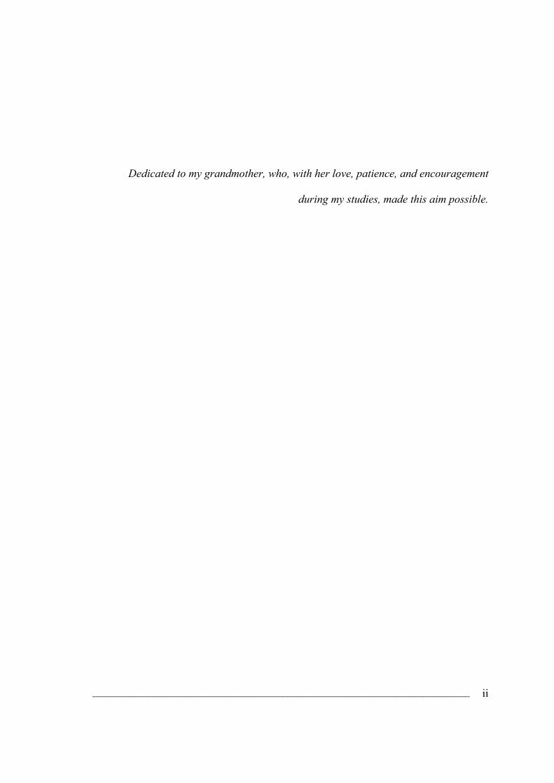
According to this configuration, the vehicle dynamics can be introduced. The latter can
be subdivided into longitudinal, lateral and vertical one, Figure 2.3 [15, 16]. Obviously,
these subsystems are not independent of each other but mutually interconnected.
While vertical dynamics are experienced by the driver in a more or less passive manner,
horizontal dynamics comprising longitudinal and lateral dynamics are actively
controlled by the human driver.
Numerous approaches to dynamics vehicle modelling are documented in the literature.
Two simple ones are adopted here to describe longitudinal and lateral Behaviour, as in
the following chapters will be presented.
Figure 2.3: Basic Structure of Vehicle System Dynamics1
1 For the meaning of few variables mentioned to see 4th and 5th chapters.
Longitudinal Dynamics
(Longitudinal Motions and
Wheel
Lateral Dynamics
(Lateral, Yawing,
and Steering Motions)
Vertical Dynamics
(Vertical oscillations,
Wheel Motions, Pitching and
Rolling)
Longitudinal Acceleration
and Deceleration
Lateral Acceleration
Cornering Resistence
Vehicle Speed
Wheel Loads
Brake Pedal Forces
Acceler. Pedal Position and Gear Shift
Steering Wheel Angle
D R I V E R
DISTURBANCESVehicle Non-linearity,
Alternating Friction Conditions Aerodynamic Forces Road Unevenness

_________________________________________________________________________________ 15
Chapter 3
3 Vehicle Dynamics Modelling
This chapter provides information on dynamics modelling of the vehicle. The vehicle
axis system used throughout the simulation is according to the SAE standard, as
described in SAE J670e [17]. As well a research study of typical forces acting at wheels
of each vehicle will be used in this research in order to construct a complete vehicle
model.
3.1 Axis System
At any given instant of time, a vehicle is subjected to a single force acting at some
location and in some direction. This so-called external or applied force maintains the
velocity or causes an acceleration of the vehicle. This force is made up of tyre,
aerodynamic, and gravitational components. These different components are governed
by different physical laws ant it is not convenient to deal with this single force.
Furthermore, these various components act at different locations and in different
directions relative to the vehicle chassis.
In order to study the vehicle performance it is necessary to define axis systems to which
all the variables, such as the acceleration, velocity and many other can be referred.
Throughout this thesis, the axis systems used in vehicle dynamics modelling will be
according to SAE J670e [17]. These two axis systems are used as required for the
Vehicle Dynamics Modelling_____________________________________________________________
_________________________________________________________________________________ 16
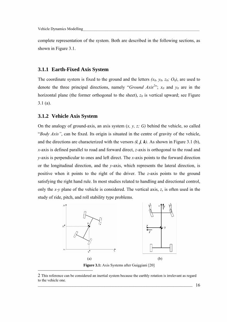
complete representation of the system. Both are described in the following sections, as
shown in Figure 3.1.
3.1.1 Earth-Fixed Axis System
The coordinate system is fixed to the ground and the letters (x0, y0, z0; O0), are used to
denote the three principal directions, namely “Ground Axis2”; x0 and y0 are in the
horizontal plane (the former orthogonal to the sheet), z0 is vertical upward; see Figure
3.1 (a).
3.1.2 Vehicle Axis System
On the analogy of ground-axis, an axis system (x, y, z; G) behind the vehicle, so called
“Body Axis”, can be fixed. Its origin is situated in the centre of gravity of the vehicle,
and the directions are characterized with the versors (i, j, k). As shown in Figure 3.1 (b),
x-axis is defined parallel to road and forward direct, z-axis is orthogonal to the road and
y-axis is perpendicular to ones and left direct. The x-axis points to the forward direction
or the longitudinal direction, and the y-axis, which represents the lateral direction, is
positive when it points to the right of the driver. The z-axis points to the ground
satisfying the right hand rule. In most studies related to handling and directional control,
only the x-y plane of the vehicle is considered. The vertical axis, z, is often used in the
study of ride, pitch, and roll stability type problems.
(a) (b)
Figure 3.1: Axis Systems after Guiggiani [20] 2 This reference can be considered an inertial system because the earthly rotation is irrelevant as regard to the vehicle one.

Vehicle Dynamics Modelling_____________________________________________________________
_________________________________________________________________________________ 17
The following list defines relevant definitions for the variables associated with this
research:
Longitudinal direction: forward moving direction of the vehicle. There are two different
ways of looking at the forward direction, one with respect to the vehicle body itself, and
another with respect to a fixed reference point. The former is often used when dealing
with acceleration and velocity of the vehicle. The latter is used when the location
information of the vehicle with respect to a starting or an ending point is desired.
Lateral direction: sideways moving direction of the vehicle. Again, there are two ways
of looking at the lateral direction, with respect to the vehicle and with respect to a fixed
reference point. Researchers often find this direction more interesting than the
longitudinal one since extreme values of lateral acceleration or lateral velocity can
decrease vehicle stability and controllability.
Sideslip angle: is the angle between the x-axis and the velocity vector that represents the
instantaneous vehicle velocity at that point along the path, as shown in Figure 3.2. It
should be emphasized that this is different from the slip angle associated with tyres.
Even though the concept is the same, each individual tyre may have a different slip
angle at the same instant in time. Often the body slip angle is calculated as the ratio of
lateral velocity to longitudinal velocity.
Tyre slip angle: This is equivalent to heading in a given direction but walking at an
angle to that direction by displacing each foot laterally as it is put on the ground as
shown in Figure 3.3. The foot is displaced laterally due to the presence of lateral forces.
Figure 3.4 shows the standard tyre axis system that is commonly used in tyre modelling.
It shows the forces and moments applied to the tyre and other important parameters
such as slip angle, sideslip angle, and others.
Figure 3.2: Sideslip Angle after Guiggiani [20].

Vehicle Dynamics Modelling_____________________________________________________________
_________________________________________________________________________________ 18
Figure 3.3: Walking Analogy to Tyre Slip Angle after Milliken [18].
In order to simplify the vehicle model so that results of the integration can be quickly
calculated, the effects of camber angle are not included in this study.
3.2 Mechanism of Pneumatic Tyres
3.2.1 Force Acting Between Road and Wheel
The wheels of all modern motor vehicles are provided with pneumatic tyres, which
support the vehicle and transfer the driving power (power tractive) through the wheel-
ground contact. Therefore in all modern vehicles all the disturbance forces which are
applied to the vehicle, with the exception of aerodynamic force, are generated in the
same contact surface.
This interaction determines how the vehicle turns, brakes and accelerates. As our
purpose is to understand the principal aspects of the vehicle dynamics, the tyre
behaviour is an essential part of this work, and in the following section its
characteristics will be explained.
In the study of the behaviour of the wheel, it is essential to evaluate the forces and the
moments acting on it. Consequently, to describe its characteristics, it is necessary to
define an axis system that serves as a reference for the definition of various parameters.
Again, one of the common axis systems used in the vehicle dynamics work has been
defined recommended by the Society of Automotive Engineers is shown in Figure 3.4

Vehicle Dynamics Modelling_____________________________________________________________
_________________________________________________________________________________ 19
Figure 3.4: SAE Tyre Axis System after Gillespie [19].
[17, 18]. The origin of the axis system is in the centre of the tyre contact and the x-axis
is the intersection of the wheel plane and the ground plane with positive direction
forward. The z-axis is perpendicular to the ground plane with a positive. Consequently,
the Y-axis is in the ground, and its direction is chosen to make the system axis
orthogonal and right hand.
Assuming all the forces to be located at the centre of contact area, we can individuate
three forces and three moments acting on the tyre from the ground. Tractive force (or
longitudinal force) Fx is the component in the x direction of the resultant force exerted
on the tyre by the road. Lateral force Fy is the component in the y direction, and normal
force Fz is the component in the z direction. Similarly, the moment Mx is the moment
about the X axis exerted from the road to the tyre. The rolling resistent moment My is
the moment about the Y axis, and the aligning torque Mz is the moment about the z-axis.
The moment applied to the tyre from the vehicle, exactly by powertrain, about the spin
axis is referred to as wheel torque Tw.
There are two important angles associated with a rolling tyre: the slip angle and the
camber angle. Slip angle α is the angle formed between the direction of the velocity of
the centre of the tyre and the plane x-z. Moreover, the camber angle γ is the angle
formed between the x-z plane and the wheel plane. How the lateral force will be shown
at the tyre-ground contact patch is a function of the slip angle and the camber angle
[22].

Vehicle Dynamics Modelling_____________________________________________________________
_________________________________________________________________________________ 20
3.2.1.1 Rolling Radius
Consider a wheel rolling on a level road with no braking or tractive moment applied to
it, with its plane perpendicular to the road. Therefore, remembering the known
relationship between the angular velocity of a rigid wheel and the forward speed as
being u=ωR, for a tyre an effective rolling radius Rr can be defined as the ratio between
the same velocity but referring to the wheel:
w ru Rω= ( 3.1)
where Rr is the effective rolling radius and ωw the velocity of the wheel. See references
[22, 23].
This relationship comes from an important assumption, called Low of Coulomb. In
accordance to this relation (called rolling without drifting), no drift between the two
parts is assumed. The behaviour of the tyre comes from this assumption and being a
point of contact3. For this reason, as shown in Figure 3.5 the centre of instantaneous
rotation R is not coincident with the centre of contact A.
Figure 3.5: Geometrical Configuration and Peripheral Speed in the Contact Zone.
3 Actually, when two surfaces make contact, the local deformation is never about a point but there is always a degeneration into a surface owing to Hertz’s Deformation.
Vehicle Dynamics Modelling_____________________________________________________________
_________________________________________________________________________________ 21
The peripheral velocity of any point varies periodically in according with the angular
variation of the wheel. Analyzing the strain around the point of contact A and knowing
the direct correlation between the radius and the linear velocity, it is possible to note the
corresponding smaller radius, in owing of the compression and consequently the
velocity decreases. In the opposite way, on the right and the left of the same point the
velocity remains meanly constant.
As a consequence of this mechanism, the spin speed of the wheel with the pneumatic
tyre is smaller than a rigid wheel with the same load. On account of the strain, this
relationship is available:
l rR R R< < ( 3.2)
The effective rolling radius depends on many factors, some of which are determined by
the tyre structure and others by the working conditions such as inflation pressure, load,
speed, and others [22, 23].
In the following work, an estimation of the resistent rolling radius will be made, in
accordance with the geometrical values assumed for the test vehicle.
3.2.1.2 Rolling Resistent
Consider a wheel rolling freely on a flat surface. If both the wheel and the road were
perfectly undeformable, there would be no resistance and consequently no need to exert
a tractive force. In the real world, as shown in the former section, perfectly rigid bodies
do not exist and both the road and the wheel are subject to deformation with the contact
surface.
During the motion of the system, how in all mechanical real system subject to strains,
the material behaviour is never perfectly elastic, but it includes at least a small plastic
strain in owing to the hysteresis of material and other phenomena. For this reason to
every turn of the wheel in according with this macroscopic deformation it is necessary
to spend some energy. This energy dissipation is what causes rolling resistent.
Obviously it increases with the tyre deformation, stiffness of the tyre and many others
parameters.

Vehicle Dynamics Modelling_____________________________________________________________
_________________________________________________________________________________ 22
Other mechanisms, like small sliding between road and wheel and aerodynamic drag are
responsible for a small contribution to the overall resistent, of the order of a small
percentage.
The distribution of the contact pressure, which at standstill was symmetrical with
respect to the centre of contact zone, becomes unsymmetrical when the wheel is rolling
and the resultant Fz moves forward producing a torque My=-Fz∆x with respect to the
rotation axis.
Rolling resistance is defined by the mentioned SAE document J670e as the force which
must be applied to the centre of the wheel with a line of action parallel to the x-axis so
that its moment about a line through the centre of tyre contact and parallel to the spin
axis of the wheel will balance the moment of the tyre contact force about this line.
Consider a free rolling wheel on level road with its mean plane coinciding with x-z
plane (γ=0, with γ camber angle), as shown in Figure 3.6.
Assuming that no traction or braking moment other than Mf due to aerodynamic drag is
applied to the wheel, the equilibrium equation about the centre of the wheel in steady
state rolling, solved in the rolling resistance Fx, is
z fx
l
F x MF
R− ∆ +
= ( 3.3)
where it must be noted that both rolling resistance, Fx, and drag moment Mf are
negative. Equation (3.3) is of limited practical use, as ∆x and Mf are not easily
determined.
For the practical purposes, rolling resistance is usually expressed as
x r zF f F= ( 3.4)
where the rolling resistance coefficient fr should be determined experimentally. The
latter depends on many parameters, as the traveling speed (or longitudinal linear
velocity of the wheel), the inflation of pressure p, the normal force Fz, the size of the

Vehicle Dynamics Modelling_____________________________________________________________
_________________________________________________________________________________ 23
Figure 3.6: (a)Wheel Deformation in owing to Rolling Resistent (Ground Deformation and Elastic
Return); (b) Forces and Contact Pressure σz in a Rolling Wheel.
tyre, the working temperature, the road conditions and finally, the forces Fx and Fy
exerted by the wheel4.
The most important effect on the rolling resistance coefficient is the longitudinal
velocity of the centre of the wheel5. Generally, this coefficient increases with the
velocity of the vehicle, at the beginning very slowly and then at an increased rate.
This functional dependence can be approximated with a polynomial of the type
0
ni
r ii
f f u=
= ∑ ( 3.5)
Where ui is the longitudinal velocity of the vehicle with i which denotes the degree of
the polynomial used and fi a coefficient valuated by experimental tests.
Generally a polynomial with second order is preferred. In this work the latter
approximation will be used. 2
0rf f Ku= + ( 3.6)
4 The complex relationships between the design and operational parameters of the tyre and its rolling resistance make it extremely difficult, if not impossible, to develop an analytic method for predicting the rolling resistent. To provide a uniform basis for collecting experimental data, the Society of Automotive Engineers recommends rolling resistent measurement procedures for various types on different surfaces, which may be found in SAE Handbook. 5 For a vehicle seen as a single rigid body and in presence of rigid driveline the velocity of the centre of the wheel (or peripheral one)can be approximated with the velocity of the vehicle.

Vehicle Dynamics Modelling_____________________________________________________________
_________________________________________________________________________________ 24
Particularly the values of f0 and K must be measured on any particular tyre. The values
assumed by these coefficients will have chosen according with Reference [22]; for more
details see [23, 24] too.
3.2.1.3 Adherence Condition of Tyre
According with Coulomb Hypothesis, before illustrated, the contact between the wheel
and the ground is without drift if this relationship is satisfied:
x s zF f F≤ ( 3.7)
where Fx and Fz are the component of tangential and normal force transferred in the
contact point respectively; as well fs represents the static friction coefficient which
depends on the surfaces of materials.
Moreover, if the former relationship (3.7) is not satisfied between both surfaces the drift
will have produced. During this critical condition, it is available in the following one
d zxF f F= ( 3.8)
where fd represents the sliding friction coefficient which depends on the surfaces of the
materials.
Therefore it is introduced an important parameter, longitudinal feed U which is able to
describe the imperfect elasticity through the bodies
1 r rx U f R∆ = = ( 3.9)
where the symbol fr had just defined.
This kind working hypothesis is able to investigate with a good approximation the
principal aspects of the dynamics behaviour of the tyre, for all its simplicity.

Vehicle Dynamics Modelling_____________________________________________________________
_________________________________________________________________________________ 25
3.2.1.4 Slope Resistance
Not taking into account a level road (banked surfaces) but a slope surface, an additional
contribution will be presented. In fact, the road grade will contribute directly to the
braking effort, either in a positive sense (uphill) or negative (downhill).
Grade is defined as the ratio of the vertical distance to the horizontal one. The additional
force on the vehicle arising from the slope, Fs, is given by:
sins xF W W θ= = ( 3.10)
For small angles typical of most grades, it is assumed that:
cos 1sin tan i
ϑϑ ϑ
== =
( 3.11)
Thus, a grade of 4% (i=0.04) will be equivalent to a deceleration of ±0.04g (with g
means the acceleration of gravity) [19].
3.2.1.5 Force Acting on the vehicle
Determining the axle loadings on a vehicle under general conditions can be performed
through the Newton’s Second Law. It is an important step in analysis of the dynamic
behaviour of the vehicle because the axle loads determine the tractive effort obtainable
at each axle, affecting the acceleration, gradeability, maximum speed, and many other
factors. The major external forces acting on a two-axle vehicle are shown in Figure 3.7.
References [22, 23, 24, 25].
In the longitudinal direction, the typical forces acting on the vehicle are caused by
different nature. For this reason, most of these forces do not act at the centre of gravity
of the vehicle, and thus create moments.

Vehicle Dynamics Modelling_____________________________________________________________
_________________________________________________________________________________ 26
Figure 3.7 Generalized Forces Acting on the Vehicle.
Referring to the same figure, the forces can be justified in the following manner:
W: weight of the vehicle acting at its centre of gravity, G, with a magnitude equal to its
mass times the acceleration of gravity. On a grade it may have two components, a
longitudinal component which is proportional to the sine of the slope and parallel to
the road, and a vertical component which is proportional to the cosine of the slope and
perpendicular to the road surface;
mv: mass of the vehicle;
Jw,f and Jw,r: Inertia of the front and rear wheels;
d2x/dt2: linear acceleration of the vehicle along the longitudinal axis;
d2θf/dt2 and d2θr/dt2: angular accelerations of the vehicle along the spin z-axis at the
front and rear wheels; Formally, they are equal and fixed to d2x/dt2 times Rr;
l: wheelbase of the vehicle, that means the length between the two spin axles;
l1 and l2: centre of gravity location, referring to both axles;
l3: distance between the vertical drawbar load and rear axle;
Fxa, Fza and Mya: Aerodynamic forces acting on the body of the vehicle. ; the former, in
x direction, may be represented as acting at a point above the ground indicated by the
height, h2, or by a longitudinal force of the same magnitude in the ground plane with
an associate moment equivalent to Fxa times h2; Instead Mya represent the
aerodynamic pitching moment;

Vehicle Dynamics Modelling_____________________________________________________________
_________________________________________________________________________________ 27
h1 and h2: lengths between the line of action of the inertia force and the aerodynamic
one, respectively;
∆x1 and ∆x2: characteristic lengths between the line of action of the inertia force and the
aerodynamic one, respectively;
Rr1 and Rr2: Rolling radius of the front and rear wheels, respectively. However, their
magnitude is always equal and so, it is fixed as Rr;
Fx1, Fx2: Rolling resistance of the front and rear tyres;
Fz1, Fz2: Vertical load of the vehicle at the front and rear tyres;
Fxd, Fzd: Drawbar loads. Exactly, they are the longitudinal and vertical forces acting at
hitch point when the vehicle is towing a trailer;
To valuate the normal components of the contact ground-tyre at both axis of the vehicle
two equations of dynamics equilibrium are required. Always referring to the same
figure, taking into account that at each axle there are two wheels, an rotational
equilibrium about the point P and a global one in forward direction have been made:
( ) ( )( ) ( )
1 , , , , 2 1 2 3 1 1 2
1 1 1 1 1
2 2 2
0v w f w f w r w r z zd xd xa
za ya x z
m xh J J F l x x F l l x F h F h
F l x M W h W l x
θ θ+ + − −∆ +∆ + + +∆ + + +
− +∆ − + + +∆ =
&& &&&& ( 3.12)
Where, for simplicity it is assumed null the contribution of the aerodynamic forces Fza
and Mya, different from the x-direction:
00
za
ya
FM
==
( 3.13)
Analogy for the both drawbar forces, that is the vehicle is running without trailer (Fxd=
Fxd=0); Therefore, it is assume that the inertia of the wheels have the same magnitude,
like as the characteristic lengths:
, ,
1 2
w f w r wJ J J
x x U
= =
∆ = ∆ = ( 3.14)

Vehicle Dynamics Modelling_____________________________________________________________
_________________________________________________________________________________ 28
Finally, like working hypothesis the elementary rotation of the wheels at the same axle
assumes equal values:
, ,w f w r wθ θ θ= = ( 3.15)
Thus, the equation of equilibrium around the point P becomes:
( )1 2 2 1 14 2 0v w w z xa x zm xh J F l F h W h W l Uθ+ − + + + + =&&&& ( 3.16)
where Wx and Wz represent the both components of the vehicle weight that, supposing
the vehicle moving on roads with small slope we have:
sincos
x v
z v
W W m giW W m g
θθ
= == =
( 3.17)
Finally, the equation which is able to provide the rear load transfer on the tyre is:
( )2 1 2 1 11 42z v w w xa v vF m xh J F h m gh i m g l Ul
θ⎡ ⎤= + + + + +⎣ ⎦&&&& ( 3.18)
Analogously, performing an equilibrium into vertical direction it is possible to obtain
the front load6 transfer:
2 12 2 0z z zd za zF F F F W+ − + − = ( 3.19)
where, for the same considerations about the drawbar and aerodynamic forces:
21
22
v zz
m g FF −= ( 3.20)
6 The same expression for the front load transfer could be obtained performing the same rotational equilibrium about the point of contact ground-tyre at the rear wheel. Evidently, it would be more industrious, mathematically.

Vehicle Dynamics Modelling_____________________________________________________________
_________________________________________________________________________________ 29
To note how the front and rear vertical loads are constituted by two parts, first “Static
Load” and “Dynamic Load”. In fact, examining the Equations (3.16) and (3.18), they
can be written as:
1
2
1 1 2 1
2 1 2 1
1 421 42
z
z
sz v w w xa v v
sz v w w xa v v
F F m xh J F h m gh i m gUl
F F m xh J F h m gh i m gUl
θ
θ
⎡ ⎤= − + + + +⎣ ⎦
⎡ ⎤= + + + + +⎣ ⎦
&&&&
&&&&
( 3.21)
where the terms Fsz1 and Fs
z2 represents the front and rear static loads transfer,
respectively; expressly they assume the following form7:
1
2
2
1
2
2
z
z
sv
sv
lF m gl
lF m gl
=
= ( 3.22)
Instead, to valuate the longitudinal components of the contact forces another two
dynamic equation of equilibrium are required. First, taking care a single axle, and
rearranging all the forces acting at its we have the Figure 3.8.
Figure 3.8: Generalized Forces Acting on the Vehicle.
7 To note that in many books concerning the Vehicle Dynamics, the static load is characterized by a proportionality respect to the semi-wheelbase, but the latter is reported only on the wheelbase total. The reason why the static load transfer is referred to the double wheelbase is corresponding to have considered on the same axle both wheels. Exactly, if the variation of the rolling resistance is considered invariant with the velocity, in the load transfer could be added this latter term.

Vehicle Dynamics Modelling_____________________________________________________________
_________________________________________________________________________________ 30
Performing an equilibrium about the spin axle of the front wheel, the relation assumes
the following form:
1 1 0w w z x rJ F U F Rθ + + =&& ( 3.23)
and, rearranging to have the value of the normal rear force:
11
w w zx
r
J F UFR
θ += −
&& ( 3.24)
Consequently, the global equilibrium at the vehicle in forward direction gives the
following relation:
1 22 2 0v x x xa xd xm x F F F F W− − + − + =&& ( 3.25)
But, with the same observations made for the former equations, we obtain:
( )2 112x v v xa xF m x m gi F F= + + +&& ( 3.26)
where Hf and Vf are the horizontal and vertical components of the reactions exerted on
the chassis by the tyre.
Finally, since the principal purpose of the model is to investigate the response of the
dynamic behaviour of the vehicle with the interaction of the powertrain, the Equations
from (3.16) to (3.22) need to be rearranged in respect of the angular engine velocity,
variable obtained from the longitudinal model. To do this it required recalling various
terms which are compared in these equations. Simplifying into the following sentences,
they can be reported. 2
2 2 2 2 c de r
c d
c dx e r
c d
c dw e
r c d
u x R
a x R
xR
η ηωτ τ
η ηωτ τ
η ηθ ωτ τ
⎛ ⎞= = ⎜ ⎟
⎝ ⎠
= =
= =
&
&&&
&&&& &
( 3.27)
Obviously, it is reported the square velocity because the aerodynamic force is
proportional to its. Therefore, the final equation which describes the tyre behaviour is:

Vehicle Dynamics Modelling_____________________________________________________________
_________________________________________________________________________________ 31
( ) ( )
( ) ( )
22 2
2 2 1 1 1
22 2
1 2 1 1 2
22 2
1 2 1
1 1 42 2
1 1 42 2
1 12 2
c d c dz r e v r w e v
c d c d
c d c dz r e v r w e v
c d c d
c dx r e v
c d
F SCxh R m hR J m g hi l Ul
F SCxh R m hR J m g hi l Ul
F SCxh R m hRl
ηη ηηρ ω ωτ τ τ τ
ηη ηηρ ω ωτ τ τ τ
ηηρ ωτ τ
⎡ ⎤⎛ ⎞⎢ ⎥= + + + + +⎜ ⎟⎢ ⎥⎝ ⎠⎣ ⎦⎡ ⎤⎛ ⎞⎢ ⎥=− + + + − +⎜ ⎟⎢ ⎥⎝ ⎠⎣ ⎦
⎛ ⎞=− +⎜ ⎟
⎝ ⎠
&
&
( )
( ) ( )( )
1 2
22 22
2 1 1 2
2 2 2
1 2 2 22 2 2
c dr w e v r
r c d
c d c dx r e v r w e v r
c d r c d
l J m g hi l U lfR
h l lF SCxR h l m R J m g h l i l U lfl R
ηη ωτ τ
ηη ηηρ ω ωτ τ τ τ
⎡ ⎤⎛ ⎞⎛ ⎞⎢ ⎥+ + + − + +⎜ ⎟⎜ ⎟⎜ ⎟⎢ ⎥⎝ ⎠⎝ ⎠⎣ ⎦⎡ ⎤⎛ ⎞⎛ ⎞ ⎛ ⎞⎛ ⎞⎢ ⎥=− − + − + + + − − + +⎜ ⎟⎜ ⎟ ⎜ ⎟⎜ ⎟ ⎜ ⎟⎝ ⎠⎢ ⎥⎝ ⎠⎝ ⎠ ⎝ ⎠⎣ ⎦
&
&
( 3.28)
3.2.2 Constitutive Equations
In order to analyze completely the dynamic behaviour of the vehicle, it is necessary to
define the tyre behaviour at each wheel in lateral direction too. In this way other two
relations, able to define the lateral behaviour of a tyre, will be found [20, 21]. From a
general point of view the lateral forces Fyij are a function of slip angle α, camber angle γ,
longitudinal force Fxij and load transfer Fzij. Formally, the former dependence is written:
( ), , ,y p x zF Y F Fα γ= ( 3.29)
where, Yp represents the “characteristic function of the tyre”. However, the influence of
the longitudinal force and the camber angle are neglected, and thus, depending on the
variability of the lateral force Fyij by the slip angle and load transfer, we will have
different kinds of tyre model.
3.2.2.1 Linear Tyre Model
Taking into account only the functional variation about the slip angle we will formulate
the tyre model able to integrate the equation of motion, shown in Chapter 5. For this
elementary model, considering constant the vertical load, the following relation is
available:
( )y pF Y α= ( 3.30)

Vehicle Dynamics Modelling_____________________________________________________________
_________________________________________________________________________________ 32
In the following section we propose most simplified model, the linear tyre model. This
latter describes the lateral force as a linear function of the slip angle [20, 21]. This
functional link is expressed into the following relation:
ij ijy ijF Cα α= ( 3.31)
where, being αi1=αi2=αi, we have:
i iy iF Cα α= ( 3.32)
and Cαi is the tyre “cornering stiffness”, defined formally by the relation:
( )0; costz
pz
F
YC C Fα α
αα= =
∂= =
∂ ( 3.33)
From the dimensional point of view it represents a force per unit angle. For convention
is always positive. Generally, its magnitude for passenger vehicle is 105 N/rad and is
two or four times as the previous one for the formula 1 tyres. The working field is
characterized by small slip angle, which means the order of magnitude is equal to 15÷20
degrees on dry road. Figure 3.9 shows the front and rear lateral force in function of the
slip angle. Obviously, increasing the magnitude of the cornering stiffness, the
inclination of the line will increase too.
0 0.5 1 1.5 2 2.5 3 3.50
0.5
1
1.5
2
2.5
3
3.5
4
4.5
5
Late
ral F
orce
[kN
]
Slip Angle [deg]
Fy1Fy2
Figure 3.9: Lateral Force versus Slip Angle.

Vehicle Dynamics Modelling_____________________________________________________________
_________________________________________________________________________________ 33
3.2.2.2 Linear Tyre Model with Relaxation Length
To study the behaviour of the tyre during the transient condition, it cannot be utilized
the algebraic function, shown in the former section, but a differential equation is
required. From experimental tests it is appeared that the lateral force is an increasing
monotonic function which begins from zero and moves in asymptotic way to the
permanent condition. From a general point of view, once a slip angle in different to
zero, the instantaneous increasing of the lateral force is not possible [20, 21].
A simple mathematical model to describe the tyre behaviour during a transient
condition, can be described by the following differential equations:
( )yi yi pd F F Yu
α+ =& ( 3.34)
where the length d is the “relaxation length” and the function Yp(α), namely
“characteristic function”, represents the lateral force in function of the slip angle during
the steady-state condition.
It is a ordinary differential equation, non homogenous, first order, linear and with
constant coefficients8. The unknown variable of this equation is the lateral force as
function of time.
Making same considerations about the former relationship, it is possible to calculate
immediately the analytical solution:
( ) h pyi yi yiF t F F= + ( 3.35)
where, Fhyi and Fp
yi are the particular integral and the homogenous associated solution
(with i which assumes the value 1 for the front wheel and 2 for the rear ones). They
assume the values, respectively
8 Strictly, this happens only if the longitudinal velocity does not change. However, as first approximation its variability is neglected.

Vehicle Dynamics Modelling_____________________________________________________________
_________________________________________________________________________________ 34
( )
( )
exphyi
pyi p
uF t A td
F Y α
⎛ ⎞= −⎜ ⎟⎝ ⎠
= ( 3.36)
where, α is the value assumed by the slip angle during the permanent conditions and A
is integration constant. To note the dependence of the particular from the slip angle α(t).
In order to calculate the value of the constant it can be imposed the following condition:
( )0 0yiF = ( 3.37)
The solution of the differential equation is presented:
( ) ( )expyi puF t A t Yd
α⎛ ⎞= − +⎜ ⎟⎝ ⎠
( 3.38)
That, substituting the initial condition, gives:
( )pA Y α= − ( 3.39)
And finally, the solution is:
( ) ( ) ( )1 exp 1 expyi p pu sF t Y t Yd d
α α⎛ ⎞ ⎛ ⎞⎛ ⎞ ⎛ ⎞= − − = − −⎜ ⎟ ⎜ ⎟⎜ ⎟ ⎜ ⎟⎝ ⎠ ⎝ ⎠⎝ ⎠ ⎝ ⎠ ( 3.40)
where it is imposed s=ut, with s which indices the displacement covered of the wheel.
Obviously this function is an increasing monotonic function which begins from zero
and moves in asymptotic way up to the permanent condition α .
The relaxation length can be obtained by some geometrical considerations, as shown in
Figure 3.10, considering the permanent value equal to 2.4 kN. Imposing s=d the relation
available is:
( ) ( )( ) ( ) ( )1 exp 1 0.6321 yi p pF t Y Yα α= − − = ( 3.41)

Vehicle Dynamics Modelling_____________________________________________________________
_________________________________________________________________________________ 35
Therefore, the length d represents the wheel displacement required to obtain a lateral
force equal to 63 percent of the steady-state value.
Another method to obtain the relaxation length observing the following property:
( )0
y
s
dF Ypds d
α
=
= ( 3.42)
Normally, the magnitude of the relaxation length is about the rolling radius of the tyre.
Synthetically, the table 3.1 shows the cornering force influence (steady-state value) on
the relaxation length. To note its influence is very small, nearly insignificant.
0 0.2 0.4 0.6 0.8 1 1.2 1.4 1.6 1.8 20
0.5
1
1.5
2
2.5
Late
ral F
orce
[kN
]
Rounds [/]
Fy 0.63 Yp
d
Figure 3.10: Lateral Force versus Wheel Rounds in Transient Condition with Permanent Value equal to
2.4 kN.
Fy(α ) d 2.00 0.248 2.20 0.250 2.40 0.248
Table 3.1: Distance assumed with variation of Steady-State Cornering Force.

Vehicle Dynamics Modelling_____________________________________________________________
_________________________________________________________________________________ 36
3.2.2.3 Non Linear Tyre Model with Relaxation Length
To describe the tyre behaviour, it is possible to use some empirical formulas which may
not have any physical correlation with the effective behaviour of the tyre, such as the
Magic Formula [20, 21, 22, 24, 25] and other experimental tendency traduced into a
mathematical form. These empirical formulas come used to develop the mathematical
model in order to study the complete vehicle dynamics. From a general point of view
the tyre description could be just an approximation problem of an unknown analytical
function. But, anyway there will have further constraints to respect. First, the first
derivative may have some fluctuations that do not really exist. Real is the same as
saying that the second derivative will be constrained too. This aspect produces the
approximation more delicate. Another important aspect is to consider how many
parameters will have to take into account, which of these will have to be constant and
their physical meanings.
Still, the general trend is been to investigate some transcendental functions which are
depending on a finite number of parameters. The function taken into account is:
( ), 1 expy z zz
CF F FF
ααα µµ
⎛ ⎞⎛ ⎞= − −⎜ ⎟⎜ ⎟⎜ ⎟⎝ ⎠⎝ ⎠
( 3.43)
where µ represents the ratio between the normalized tyre friction and the lateral force.
Even if the lateral force depends on many factors, such as the road surface conditions,
the curves shown in Figure 3.11 and Figure 3.12 illustrate how the normal force
influences the shape of Fyi for the front and rear wheels.

Vehicle Dynamics Modelling_____________________________________________________________
_________________________________________________________________________________ 37
0 5 10 150
0.5
1
1.5
2
2.5
3
3.5
4
4.5
Late
ral F
orce
[kN
]
Slip Angle [deg]
FZ1=1kNFZ2=2kNFZ3=3kNFZ4=4kNFZ5=5kN
Figure 3.11: Front Lateral Force versus Slip Angle with Different Normal Load.
0 5 10 150
0.5
1
1.5
2
2.5
3
3.5
4
4.5
Late
ral F
orce
[kN
]
Slip Angle [deg]
FZ2=1kNFZ2=2kNFZ2=3kNFZ2=4kNFZ2=5kN
Figure 3.12: Rear Lateral Force versus Slip Angle with Different Normal Load.

_________________________________________________________________________________ 38
Chapter 4
4 Longitudinal Dynamics Model
Modelling an vehicle in all its parts requires good knowledge of the components
involved and their physics. The first step in the study of the longitudinal behaviour of
the vehicle is to create a mathematical model that must represent the physical system
with good approximation. This chapter describes the modelling of the dynamics
longitudinal. In the field of vehicle lateral dynamics field, the feed velocity is kept
constant in order to investigate the behaviour of the rest of the system. In this vehicle
model, the speed and torque variability have been added.
4.1 Physical Model
From a mechanical point of view, a vehicle can be mainly presented as a numerous set
of rotating and translating parts. Initially, to identify its dynamic behaviour we will
model the whole system, basically composed of the propulsion system called
“powertrain” and the set including the suspension, wheel and road links, called
“chassis”.
According to the aim to reach, vehicles can be modeled in many different ways. In fact,
in this work we are going to analyze the dynamic development of the vehicle speed
from a known throttle opening.
That is the reason why we will consider engine modelling only, and not driveline
modelling [19], as shown in Figure 4.1.

Longitudinal Dynamics Model____________________________________________________________
_________________________________________________________________________________ 39
Figure 4.1: Primary Elements in the Powertrain
Schematically, the powertrain system can be represented as in Figure 4.2. The system-
vehicle can be configured through a set of interconnected blocks; see Figure 4.3 for a
description of the different powertrain components [26, 27].
Figure 4.2: Schematization Elements in the Powertrain
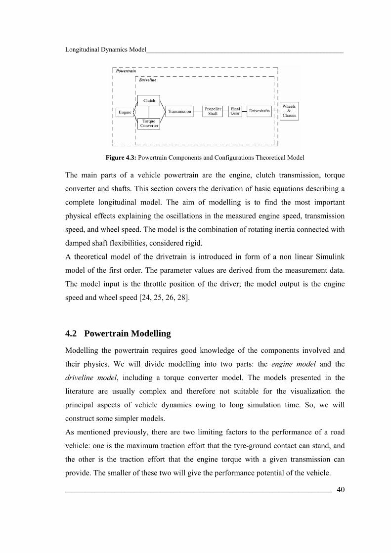
Longitudinal Dynamics Model____________________________________________________________
_________________________________________________________________________________ 40
Figure 4.3: Powertrain Components and Configurations Theoretical Model
The main parts of a vehicle powertrain are the engine, clutch transmission, torque
converter and shafts. This section covers the derivation of basic equations describing a
complete longitudinal model. The aim of modelling is to find the most important
physical effects explaining the oscillations in the measured engine speed, transmission
speed, and wheel speed. The model is the combination of rotating inertia connected with
damped shaft flexibilities, considered rigid.
A theoretical model of the drivetrain is introduced in form of a non linear Simulink
model of the first order. The parameter values are derived from the measurement data.
The model input is the throttle position of the driver; the model output is the engine
speed and wheel speed [24, 25, 26, 28].
4.2 Powertrain Modelling
Modelling the powertrain requires good knowledge of the components involved and
their physics. We will divide modelling into two parts: the engine model and the
driveline model, including a torque converter model. The models presented in the
literature are usually complex and therefore not suitable for the visualization the
principal aspects of vehicle dynamics owing to long simulation time. So, we will
construct some simpler models.
As mentioned previously, there are two limiting factors to the performance of a road
vehicle: one is the maximum traction effort that the tyre-ground contact can stand, and
the other is the traction effort that the engine torque with a given transmission can
provide. The smaller of these two will give the performance potential of the vehicle.

Longitudinal Dynamics Model____________________________________________________________
_________________________________________________________________________________ 41
In low gears with the engine throttle fully open, the traction stress may be limited by the
nature of the tyre-road grip. Instead, in higher gears, the traction effort is usually
determined by the engine and transmission characteristics. To predict the overall
performance of a vehicle, the engine and transmission characteristics must be taken into
consideration. In this section, the general characteristics of vehicle power and
transmissions will be presented.
4.2.1 Engine Model: Characteristics of Internal Combustion Engines
As most road vehicles are powered by reciprocating internal combustion engines, their
characteristics will be summarized in the present section.
Apart from the action of the throttle control, the power supplied by the engine depends
mainly on the rotational speed. The performance of an internal combustion engine is
usually summarized in a single map plotted in a plane whose axles are the rotational
speed ωe and the torque (or power Pe) as shown in Figure 4.4. Often the former is
reported in rpm and the latter in Nm (or in kw if power); in the present text however S.I.
units, i.e. rad/s will be used, according to the following relation:
260
ee
nπω = ( 4.1)
with ne that represents the engine speed in rad/s.
The choice about the characteristic representation does not make sense because power
and torque are related by the speed. Specifically,
e e eP T ω= ( 4.2)
where Pe is the engine power.
The internal combustion engine is connected to the wheels through a transmission
system which includes a clutch, a gear selector (or gear box) and some joints.
The relationship between the angular velocity of the engine and the velocity of the
wheels is simply given by:

Longitudinal Dynamics Model____________________________________________________________
_________________________________________________________________________________ 42
c de w
c d
τ τω ωη η
= ( 4.3)
where τc and τd are the transmission ratios (defined as the ratio between the velocities of
the output and the input shafts) of the gearbox and the final drive respectively.
Moreover, ηc and ηd are the efficiency of the gearbox and the final drive. Note that the
transmission ratio and the efficiency of the gearbox are a function of gear in. Instead,
the other parameters of the final drive are constant. The efficiency of the gearbox is
usually smaller than 1.
However, the relationship between the angular velocity of the wheels and the velocity
of the vehicle is given from the Equation (3.1), shown in the following relationship:
w ru Rω= ( 4.4)
where Rr is the effective rolling radius.
This model can be considered as the first important aspect of the complete vehicle
model. The characteristic curve of an internal combustion engine defines the torque
supplied as function of the engine speed ne and throttle opening α that is as function of a
parameter able to show how much the throttle should be opened.
Conceptually, the throttle opening is proportional to the mass flow rate of air. In fact,
the throttle opening assumes included values between 0, section completely closed and
1 (or percent value) for fully opened.
Usually, the output engine torque is measured with a test-engine linked to a brake
system, in maximum and minimum admissions. During these two steady-state
conditions, the corresponding characteristic curves can be pointed out . A representative
characteristic of the gasoline engine is shown in Figure 4.4 and 4.5, in dimensionless
form.

Longitudinal Dynamics Model____________________________________________________________
_________________________________________________________________________________ 43
0 500 1000 1500 2000 2500 3000 3500 4000 4500 5000-100
-50
0
50
100
150
200
250Engine map
Engine Speed [rpm]
Eng
ine
Torq
ue [N
m]
th=0th=0.2th=0.3th=0.4th=0.5th=0.6th=0.7th=0.8th=0.9th=1
Figure 4.4: Performance Characteristic of Test-Vehicle
0 0.1 0.2 0.3 0.4 0.5 0.6 0.7 0.8 0.9 1-0.4
-0.2
0
0.2
0.4
0.6
0.8
1Dimensionless Engine map
ne/nemax [/]
T e/Tem
ax [/
]
th=0th=20%th=30%th=40%th=50%th=60%th=70%th=80%th=90%th=100%
Figure 4.5: Dimensionless Performance Characteristic of Test-Vehicle

Longitudinal Dynamics Model____________________________________________________________
_________________________________________________________________________________ 44
Numerically, this picture is an element matrix because it represents the engine torque as
function of the engine speed for a fixed throttle opening.
In intermediate conditions, with a good approximation, the engine torque is a linear
function of throttle opening, so the engine torque is expressed by the following relation:
( )max min 1e e eT T Tα α= + − ( 4.5)
where Temax and Temin represent the maximum and minimum value of the engine torque
Te, [24].
4.2.2 Gear Box and Torque Converter
These two models will be illustrated directly in the Chapter 6, with the main details. The
complete gearbox is simulated. The presence of the clutch is neglected.
4.3 Driver Model
A driver typically control vehicle speed by depressing the accelerator pedal to request
positive torque or depressing the brake pedal (not modeled) to request negative torque.
In a conventional vehicle, positive torque is supplied only by the combustion engine,
and negative torque is supplied only by the brakes. Perhaps, to develop the complete
vehicle model, but not taking into account the brake model, the negative torque is
supplied by the close-throttle manoeuvreing (as well to work with negative torque
value) and the total resistent motion.
4.4 Equivalent Dynamic System
In this section, the principal aim is to reduce all the mechanical system into a reduced
system in order to work with an easier vehicle model.

Longitudinal Dynamics Model____________________________________________________________
_________________________________________________________________________________ 45
For this reason an equivalent dynamic system, including all vehicle parts, (rotating and
translating ones) will carried out. From the mathematical point of view, the Kinetics
Energy Theorem end Principle of D’Alembert will be used.
Consider a vehicle with a mechanical transmission with a number of different gear
ratios. Schematically, in according to Figure 4.2, the complex system studied, before
reducing, is shown in Figure 4.6. Note the new parameters introduced, τc, ηc, τd, ηd, Ie
and Iw.
These parameters represent a great physical mean:
Ie: Engine Inertia;
Iw: Wheel Inertia;
τc: Transmission Gear box ratio;
τd: Final drive ratio;
ηc, ηd: Gear box and Final drive efficiency. In order to reduce the whole mechanical system into an equivalent one, we can assume
that is only a physical system (without energy transferred). The vehicle can be modeled
as two moments of inertia, one to model the engine and one to model the vehicle; see
Figure 4.7 (a) and (b). The first one includes the moment of inertia of the engine, up to
the flywheel, while the moment of inertia of the clutch disks, of the shaft entering the
gearbox, of all the rotating parts, reduced to the engine shaft, and the mass of the
vehicle as “seen” from the engine are included in the second
Figure 4.6: Driveline Notations

Longitudinal Dynamics Model____________________________________________________________
_________________________________________________________________________________ 46
Figure 4.7: Driveline Complex Model. (a) Transmission Engaged; (b) Transmission Disengaged.
In accordance with our convention (RHL), we can note the opposite orientations of the
torques applied at shaft, because the first on the left is drive and the second one is
“resistent”.
To simplify the theoretical model, we start from the following working hypothesis:
• Transmission shaft is rigid, as well as the stiffness ks and has an infinite value.
This makes things easier;
• Transmission is engaged-disengaged immediately, the clutch system is
neglected. Actually, this working hypothesis is not satisfied; only making a
good setup of the implementation model, a realistic approximation can be
obtained. So, the final esteemed system is shown in Figure 4.8.
Figure 4.8: Equivalent System for a Driveline Model.

Longitudinal Dynamics Model____________________________________________________________
_________________________________________________________________________________ 47
During an acceleration manoeuvre, the rotating elements (wheels, transmission, the
engine itself) must increase their angular velocity. Resorting to this expedients, it is
possible to write only one equation, linking the engine torque with kinetic energy of the
vehicle [23, 24, 29].
Fundamental equations for the driveline will be derived by using the generalized
Newton’s second law of motion.
The state equation of the speed is given below:
e ldP Pdtτ
− = ( 4.6)
where:
τ: Kinetic Energy of the vehicle;
Ieq: Equivalent Inertia;
Te: Engine Power;
Tl: Load Power.
Note that the engine power Pe should be the one provided in non steady-state running.
The kinetic energy of the vehicle, “seen” as an equivalent system can be expressed as
2 2 2
1
1 1 12 2 2
n
i i eq ei
I m v Iτ ω ω=
= + =∑ ( 4.7)
where the sum extends to all translating elements which must be accelerated when the
vehicle speeds up. Making a derivate of the kinetic energy we obtain
212
eqeeq e e
dIdd Idt dt dt
ωτ ω ω= + ( 4.8)
Generally, the equivalent inertia changes in time if a torque converter is used because of
the transmission ratio of the gearbox. If we consider that the equivalent inertia does not
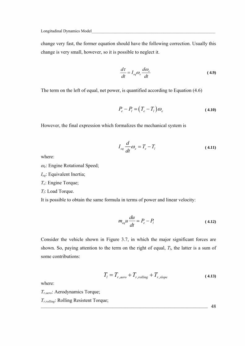
Longitudinal Dynamics Model____________________________________________________________
_________________________________________________________________________________ 48
change very fast, the former equation should have the following correction. Usually this
change is very small, however, so it is possible to neglect it.
eeq e
dd Idt dt
ωτ ω= ( 4.9)
The term on the left of equal, net power, is quantified according to Equation (4.6)
( )e l e l eP P T T ω− = − ( 4.10)
However, the final expression which formalizes the mechanical system is
eq e e ldI T Tdt
ω = − ( 4.11)
where:
ωe: Engine Rotational Speed;
Ieq: Equivalent Inertia;
Te: Engine Torque;
Tl: Load Torque.
It is possible to obtain the same formula in terms of power and linear velocity:
eq e ldum u P Pdt
= − ( 4.12)
Consider the vehicle shown in Figure 3.7, in which the major significant forces are
shown. So, paying attention to the term on the right of equal, Tl, the latter is a sum of
some contributions:
, , ,l r aero r rolling r slopeT T T T= + + ( 4.13)
where:
Tr,aero: Aerodynamics Torque;
Tr,rolling: Rolling Resistent Torque;

Longitudinal Dynamics Model____________________________________________________________
_________________________________________________________________________________ 49
Tr,slope: Slope Torque;
In our simulations, we assumed that only the slope torque is constant (not during time)
and known by the driver behaviour. In this way, there is not a direct connection between
the engine speed and the engine torque, but continuously an update for these.
In order to construct only an equation, we need an explicit form of the equivalent inertia
Ieq; it assumes the form:
, ,4eq engine r chassis r wheelI I I I= + + ( 4.14)
with:
Iengine: Engine Inertia;
Ir,chassis: Chassis Inertia;
Ir,wheel: Wheel Inertia;
4.4.1 Reduction of Forces Acting on the Vehicle
In order to integrate numerically Equation 4.11, an explicit form of the whole physical
terms, present in it, is required. This means, to perform two operations on the effective
system; see Figure 4.8, namely “Reductions of mass” and “Reduction of forces”,
applying the Kinetics Energy Theorem and Principle of D’Alembert respectively [23,
24, 29].
From a general point of view, a force Fe, applied to a generic point of the effective9
system, can be reduced10 into a force Fr, acting to the reduced system (or into a torque
Tr), only fixing a “reduction axle”. The equivalence is verified if the works carried out
by the each forces are equal. Considering dse and dsr, the displacement of the previous
points, we have the following relation:
e e r rF ds F ds= ( 4.15)
and so we obtain:
9 The forces acting on the effective system Fe are denoted through the pedics e. 10 Analogy with note 1 the forces and the torques acting on the reduced system Fr and Tr are denoted through the pedics r too.

Longitudinal Dynamics Model____________________________________________________________
_________________________________________________________________________________ 50
er e
r
dsF Fds
= ( 4.16)
Likewise, considering the reduction of a moment Tr, acting on the normal plane to the
selected axle, the elementary rotation around this latter, dθ must be considered. So, the
following relationship must be satisfied:
e e r rF ds T dθ= ( 4.17)
and so:
er e
r
dsT Fdθ
= ( 4.18)
According to this concept, all the machine members can be reduced to an equivalent
system, namely “Equivalent Flywheel”.
The external forces acting on the vehicle to develop the reduced system are:
• Aerodynamics Force in straight condition (without taking account of the positive
and negative lift);
• Rolling Force at tyre-ground contact;
• Grade Resistent (or slope force) acting in the centre of gravity.
The reduction of forces, considered as a general principle, is performed trough the
equality of the work carried out by the effective forces (acting on the effective system)
and the work carried out by the reduced ones (acting on the reduced system).
4.4.1.1 Reduction Aerodynamics Force
The aerodynamic drag is characterized by the equation:
2,
12aero e aero air xF F SC uρ= = ( 4.19)
Applying the Principle of D’Alembert to reduce this force on the engine shaft:

Longitudinal Dynamics Model____________________________________________________________
_________________________________________________________________________________ 51
, ,e
r aero e aeror
dsT Fdθ
= ( 4.20)
It is required to make the quantities dse and dθr explicit.
e eds u dt= ( 4.21)
and
rd dtθ ω= ( 4.22)
So, replacing these two expressions11 in the former:
, ,e
r aero e aerouT Fω
= ( 4.23)
From the relationship between the velocity of the vehicle and the velocity of the wheels
we obtain:
, ,w
r aero e aero re
T F R ωω
= ( 4.24)
Where parameter Rr represents the effective rolling radius. However, taking into
account of the relation of the rotational wheel velocity and the engine velocity we have
finally an expression of the reduced aerodynamics force:
2, ,
12
c d c dr aero e aero r air x r
c d c d
T F R SC R uη η η ηρτ τ τ τ
= = ( 4.25)
or like a function of the rotational wheel velocity:
11 To note that the angular velocity ω is the velocity of a flywheel with mass equal to Ir which is rotating around the reduction axle. Specially, this velocity corresponds to the rotational engine velocity because the engine shaft was chosen as “reduction axle”.

Longitudinal Dynamics Model____________________________________________________________
_________________________________________________________________________________ 52
3 2,
12
c dr aero air x r w
c d
T SC Rη ηρ ωτ τ
= ( 4.26)
and a function of the engine velocity:
3 3
3 2, 3 3
12
c dr aero air x r e
c d
T SC Rη ηρ ωτ τ
= ( 4.27)
4.4.1.2 Reduction Rolling Force
The rolling resistent force can be expressed as :
,rolling e rolling rF F f W= = ( 4.28)
where W represents the weight of the vehicle. We can obtain the same expression for
the rolling force reduced to the engine shaft:
, ,e
r rolling e rollingr
dsF Fdθ
= ( 4.29)
where the terms dse and dθr do not change.
Replacing these in the rolling resistent relation:
, ,e
r rolling e rollinge
uF Fω
= ( 4.30)
and so we finally obtain:
, ,w
r rolling e rolling re
F F R ωω
= ( 4.31)
Therefore, using the relationship between rotational wheel velocity and the engine
velocity we finally obtain an expression of the reduced rolling force too:

Longitudinal Dynamics Model____________________________________________________________
_________________________________________________________________________________ 53
, ,c d
r rolling e rolling r ec d
F F Rη η ωτ τ
= ( 4.32)
and the same expression in explicit form:
,c d
r rolling r r ec d
F Wf Rη η ωτ τ
= ( 4.33)
Where the terms have been already defined.
4.4.1.3 Reduction Grade Force
The grade force can be expressed as follows:
,slope e slopeF F Wi= = ( 4.34)
where i indicates the slope road. By applying the Principle of D’Alembert to reduce this
force on the engine shaft, we obtain again:
, ,e
r slope e sloper
dsF Fdθ
= ( 4.35)
with dse and dθr which are not chancing expression. Representing the latter quantities in
explicitly we have:
, ,e
r slope e slopee
uF Fω
= ( 4.36)
By considering the relationship between the velocity of the vehicle, the velocity of the
engine, we can obtain:
, ,w
r slope e slope re
F F R ωω
= ( 4.37)

Longitudinal Dynamics Model____________________________________________________________
_________________________________________________________________________________ 54
where the parameter Rr represents the effective rolling radius. However, taking into
account of the relation of the rotational wheel velocity and the engine velocity we have
finally an expression of the reduced aerodynamics force:
, ,c d
r slope e slope rc d
F F R η ητ τ
= ( 4.38)
and a final expression:
,c d
r slope rc d
F WR iη ητ τ
= ( 4.39)
Note that this resistent force is a constant in opposition with the other ones, and its value
changes only as function of the slope grade and not changing with the velocity.
4.4.2 Reduction of Inertias of the Vehicle
As is the case for the reduction of forces, it is possible to do the same thing, estimating
the reduced inertias of our model, applying the Kinetics Energy Theorem [23, 24, 29].
Given a point or an axle belonging to the effective system, the reduction of masses can
be performed, by substituting each mass me of the effective system for a mass mr
reduced to the point of reduction, imposing the invariance of Kinetic Energy.
By noting with ue the velocity of the effective mass (as well the point of application of
this mass) and with ur the velocity of the reduced mass (as well the point of
application), we can impose the invariance of kinetic energy:
2 21 12 2e e r rm u m u= ( 4.40)
therefore, 2
2e
r er
um mu
= ( 4.41)

Longitudinal Dynamics Model____________________________________________________________
_________________________________________________________________________________ 55
The mass me, translating with velocity ue, can be reduced to a rotating mass mr, having
velocity ω around a reduction axle, from which it is distant of r. This can be obtained by
expressing the following relationship:
2 2 21 12 2e e rm u m rω= ( 4.42)
and: 2
r rI m r= ( 4.43)
it is possible to obtain: 2 2
e e rm u I ω= ( 4.44)
and we have the final expression about the reduced inertia as function of the effective
parameters: 2
2e
r euI mω
= ( 4.45)
Naturally, an inertia flywheel whose moment of inertia is equal to Ie will be equivalent
to a flywheel, namely Ir which is rotating with velocity ω around the reduction axle,
only if the following relation is satisfied:
2 21 12 2e e rI Iω ω= ( 4.46)
And so, the other condition can be obtained by:
2
2e
r eI I ωω
= ( 4.47)
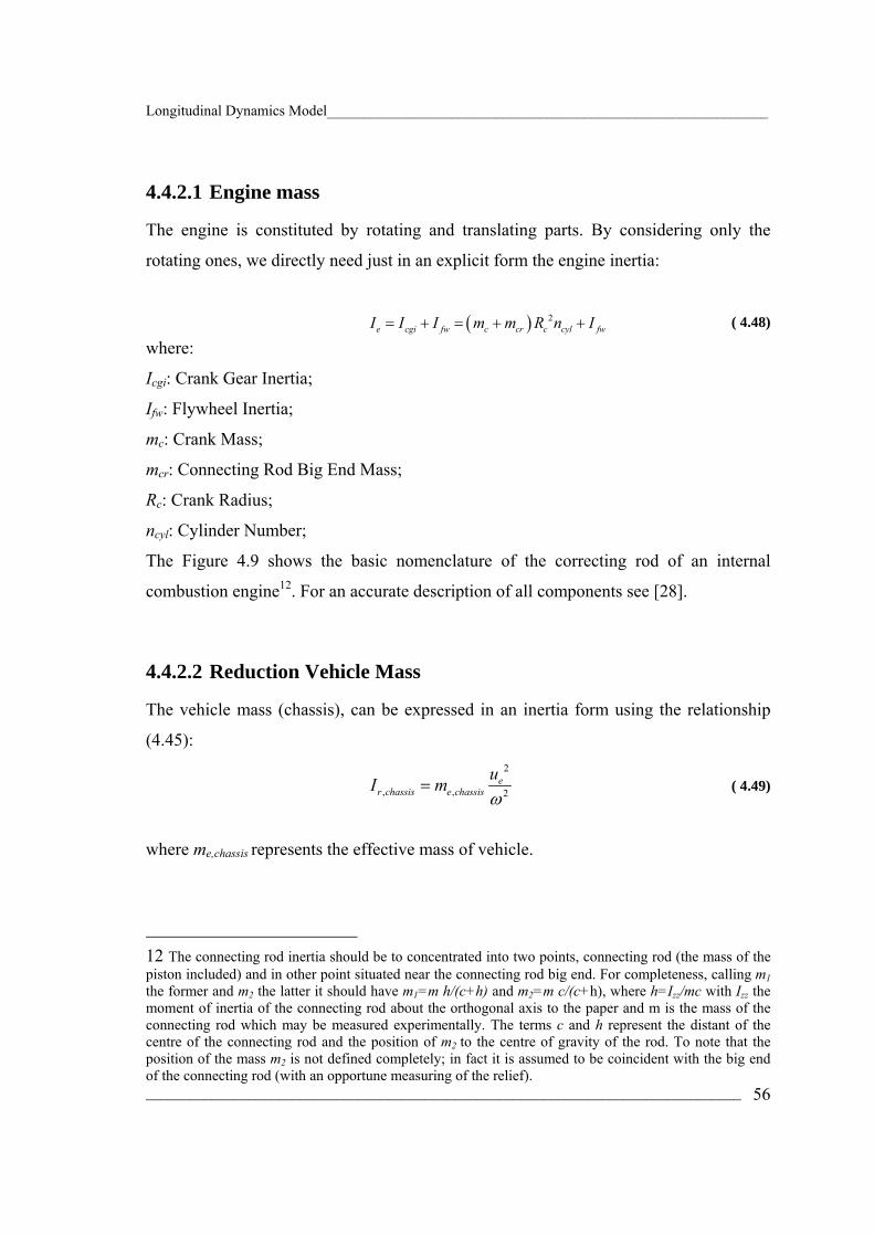
Longitudinal Dynamics Model____________________________________________________________
_________________________________________________________________________________ 56
4.4.2.1 Engine mass
The engine is constituted by rotating and translating parts. By considering only the
rotating ones, we directly need just in an explicit form the engine inertia:
( ) 2e cgi fw c cr c cyl fwI I I m m R n I= + = + + ( 4.48)
where:
Icgi: Crank Gear Inertia;
Ifw: Flywheel Inertia;
mc: Crank Mass;
mcr: Connecting Rod Big End Mass;
Rc: Crank Radius;
ncyl: Cylinder Number;
The Figure 4.9 shows the basic nomenclature of the correcting rod of an internal
combustion engine12. For an accurate description of all components see [28].
4.4.2.2 Reduction Vehicle Mass
The vehicle mass (chassis), can be expressed in an inertia form using the relationship
(4.45): 2
, , 2e
r chassis e chassisuI mω
= ( 4.49)
where me,chassis represents the effective mass of vehicle.
12 The connecting rod inertia should be to concentrated into two points, connecting rod (the mass of the piston included) and in other point situated near the connecting rod big end. For completeness, calling m1 the former and m2 the latter it should have m1=m h/(c+h) and m2=m c/(c+h), where h=Izz/mc with Izz the moment of inertia of the connecting rod about the orthogonal axis to the paper and m is the mass of the connecting rod which may be measured experimentally. The terms c and h represent the distant of the centre of the connecting rod and the position of m2 to the centre of gravity of the rod. To note that the position of the mass m2 is not defined completely; in fact it is assumed to be coincident with the big end of the connecting rod (with an opportune measuring of the relief).

Longitudinal Dynamics Model____________________________________________________________
_________________________________________________________________________________ 57
Figure 4.9: Description of Correcting Rod of Internal Combustion Engine.
As in the former section, about the reduced forces, we can have the same expression for
the reduced inertia, explaining the vehicle velocity: 2
2, , 2
wr chassis e chassis r
e
I m R ωω
= ( 4.50)
where it is still the concept about the rotational velocity ω. Substituting the relationship
between the angular velocity of the wheels for that of the engine:
2
2, ,
c dr chassis e chassis r
c d
I m R η ητ τ
⎛ ⎞= ⎜ ⎟
⎝ ⎠ ( 4.51)
4.4.2.3 Reduction Wheel Inertia
Each wheel mass can be considered as an inertia performing the relationship (4.47): 2
, , 2e
r wheel e wheelI I ωω
= ( 4.52)
where Ie,wheel is the effective inertia of the wheel. As was the case for the chassis mass,
we have the same expression for the reduced inertia of the wheel, noting that the
effective angular velocity is that of the wheel: 2
, , 2w
r wheel e wheele
I I ωω
= ( 4.53)
Therefore, by substituting the relationship between the angular velocity of the wheels
and the engine one:

Longitudinal Dynamics Model____________________________________________________________
_________________________________________________________________________________ 58
2
, ,c d
r wheel e wheelc d
I I η ητ τ
⎛ ⎞= ⎜ ⎟
⎝ ⎠ ( 4.54)
From the Equation (4.12) the maximum acceleration the vehicle is capable of at the
various speeds is immediately obtained
max
e lx
eq
P Pdu adt m u
−⎛ ⎞ = =⎜ ⎟⎝ ⎠
( 4.55)
where the engine power Pe is the maximum power that the engine can deliver at the
speed ωe related to speed u.
The plot of the maximum acceleration versus the speed for a vehicle with a five speed
gearbox is reported in Figure 4.10, and 4.11.
The minimum time needed to accelerate from speed u1 to speed u2 can be computed by
separating the variables in Equation (4.11)and integrating
2
1 2
1
ueq
u ue lu
mT udu
P P→ =−∫ ( 4.56)
The integral must be performed separately for each velocity range in which the
equivalent mass is constant because in this way the gearbox works with a fixed
transmission ratio. Although it is possible to integrate analytically Equation (4.11) if the
maximum power is a polynomial, numerical integration is usually performed.
A graphical interpretation of the integration is performed, as shown in Figure 4.12. The
area under the curve:
1 eq
x e l
m ua P P
=−
( 4.57)
versus u is the time required for the acceleration.
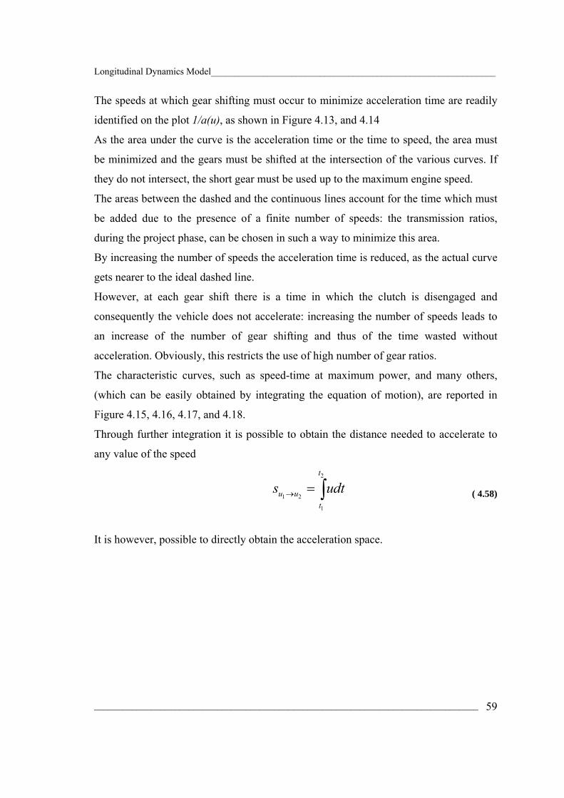
Longitudinal Dynamics Model____________________________________________________________
_________________________________________________________________________________ 59
The speeds at which gear shifting must occur to minimize acceleration time are readily
identified on the plot 1/a(u), as shown in Figure 4.13, and 4.14
As the area under the curve is the acceleration time or the time to speed, the area must
be minimized and the gears must be shifted at the intersection of the various curves. If
they do not intersect, the short gear must be used up to the maximum engine speed.
The areas between the dashed and the continuous lines account for the time which must
be added due to the presence of a finite number of speeds: the transmission ratios,
during the project phase, can be chosen in such a way to minimize this area.
By increasing the number of speeds the acceleration time is reduced, as the actual curve
gets nearer to the ideal dashed line.
However, at each gear shift there is a time in which the clutch is disengaged and
consequently the vehicle does not accelerate: increasing the number of speeds leads to
an increase of the number of gear shifting and thus of the time wasted without
acceleration. Obviously, this restricts the use of high number of gear ratios.
The characteristic curves, such as speed-time at maximum power, and many others,
(which can be easily obtained by integrating the equation of motion), are reported in
Figure 4.15, 4.16, 4.17, and 4.18.
Through further integration it is possible to obtain the distance needed to accelerate to
any value of the speed
2
1 2
1
t
u ut
s udt→ = ∫ ( 4.58)
It is however, possible to directly obtain the acceleration space.

Longitudinal Dynamics Model____________________________________________________________
_________________________________________________________________________________ 60
0 10 20 30 40 50 60 700
1
2
3
4
5
6
u [m/s]
ax [m
/s2 ]
Maximum Acceleration Diagram
1th gear2nd gear3rd gear4th gear5th gear
Figure 4.10: Maximum Acceleration as function of the Speed.
0 10 20 30 40 50 60 70
10-2
10-1
100
u [m/s]
ax [m
/s2 ]
Maximum Acceleration Diagram
1th gear2nd gear3rd gear4th gear5th gear
Figure 4.11: Maximum Acceleration as function of the Speed in log scale and reverse.

Longitudinal Dynamics Model____________________________________________________________
_________________________________________________________________________________ 61
0 10 20 30 40 50 600
0.2
0.4
0.6
0.8
1
1.2
1.4
1.6
1.8
2
u [m/s]
1/ax
[s2 /m
]
Reciprocal Maximum Acceleration Diagram
1th gear2nd gear3rd gear4th gear5th gear
Figure 4.12: Function 1/a(u) and Search for the Optimum Speeds for Gear Shifting.
Figure 4.13: Function 1/a(u) and Search for the Optimum Speeds for Gear Shifting; the white area is the
time to speed.

Longitudinal Dynamics Model____________________________________________________________
_________________________________________________________________________________ 62
0 10 20 30 40 50 6010
-2
10-1
100
u [m/s]
1/ax
[s2 /m
]
Reciprocal Maximum Acceleration Diagram
1th gear2nd gear3rd gear4th gear5th gear
Figure 4.14: Function 1/ax(u) in log scale.
0 10 20 30 40 50 60 701500
2000
2500
3000
3500
4000
4500
5000
5500
6000
6500
Vehicle Velocity [m/s]
Eng
ine
Vel
ocity
[rpm
]
Vehicle Velocity vs Engine Velocity
1th gear2nd gear3rd gear4th gear5th gear
Figure 4.15: Engine Speed versus Vehicle Speed.

Longitudinal Dynamics Model____________________________________________________________
_________________________________________________________________________________ 63
0 20 40 60 80 100 120 140 160 180 200-1
0
1
2
3
4
5
6
time [s]
ax [m
/s2 ]
Acceleration-time curve
1th gear2nd gear3rd gear4th gear5th gear
Figure 4.16: Acceleration-time curve.
0 20 40 60 80 100 120 140 160 180 2000
10
20
30
40
50
60
70
time [s]
u [m
/s]
Speed-time curve
1th gear2nd gear3rd gear4th gear5th gear
Figure 4.17: Speed-time curve.

Longitudinal Dynamics Model____________________________________________________________
_________________________________________________________________________________ 64
0 20 40 60 80 100 120 140 160 180 2000
2000
4000
6000
8000
10000
12000
time [s]
s [m
]
Distance-time curve
1th gear2nd gear3rd gear4th gear5th gear
Figure 4.18: Distance-time curve.
0 2 4 60
1000
2000
3000
4000
time [s]
Fx2
[N]
Tangential Load rear time curve
0 2 4 6-90
-85
-80
-75
-70
-65
-60
time [s]
Fx1
[N]
Tangential Load front time curve
0 2 4 62000
2500
3000
3500
4000
time [s]
Fz2
[N]
Load Transfer rear time curve
0 2 4 63000
3500
4000
4500
time [s]
Fz1
[N]
Load Transfer front time curve
1th gear2nd gear3rd gear4th gear5th gear
Figure 4.19: Traction tyre curve.

Longitudinal Dynamics Model____________________________________________________________
_________________________________________________________________________________ 65
-2 0 2 4 6 80
0.5
1
time [s]
Trac
tion
Par
amet
er
in 1
th g
ear [
/]
-2 0 2 4 6 80
0.5
1
time [s]
Trac
tion
Par
amet
er
in 2
nd g
ear [
/]
-2 0 2 4 6 80
0.5
1
time [s]
Trac
tion
Par
amet
er
in 3
rd g
ear [
/]
-2 0 2 4 6 80
0.5
1
time [s]
Trac
tion
Par
amet
er
in 4
th g
ear [
/]
-2 0 2 4 6 80
0.5
1
time [s]
Trac
tion
Par
amet
er in
5th
gea
r [/]
Traction ParameterTraction Limit
Figure 4.20: Traction Control curve.
0 50 100 150 2000
20
40
60
80
100
time [s]
Pe
[kw
]
Engine Power time curve
0 50 100 150 2000
20
40
60
80
time [s]
Pl [
kw]
Load Power time curve
0 50 100 150 2000
5
10
15
20
time [s]
Pro
lling
[kw
]
Rolling Resistent time curve
0 50 100 150 2000
10
20
30
40
50
60
time [s]
Pae
ro [k
w]
Aerodynamics Resistent time curve
1th gear2nd gear3rd gear4th gear5th gear
Figure 4.21: : Power-time curve.

Longitudinal Dynamics Model____________________________________________________________
_________________________________________________________________________________ 66
0 20 40 60 80 100 120 140 160 180 2000
100
200
300
Te [N
m]
Engine Torque time curve
0 20 40 60 80 100 120 140 160 180 2000
10
20
30
Trol
ling
[Nm
]
Rolling Torque time curve
0 20 40 60 80 100 120 140 160 180 2000
50
100
time [s]
Taer
o [N
m]
Aerodynamics Torque time curve
1th gear2nd gear3rd gear4th gear5th gear
Figure 4.22: Torque-time curve.
1000 2000 3000 4000 5000 60000
20
40
60
80
100
Engine Velocity [rpm]
Pe
[kw
]
Engine Power vs Engine Velocity
1000 2000 3000 4000 5000 60000
20
40
60
80
Engine Velocity [rpm]
Pl [
kw]
Load Power vs Engine Velocity
1000 2000 3000 4000 5000 60000
5
10
15
20
Engine Velocity [rpm]
Pro
lling
[kw
]
Rolling Resistent vs Engine Velocity
1000 2000 3000 4000 5000 60000
10
20
30
40
50
60
Engine Velocity [rpm]
Pae
ro [k
w]
Aerodynamics Resistent vs Engine Velocity
1th gear2nd gear3rd gear4th gear5th gear
Figure 4.23: Power versus Engine Velocity.

Longitudinal Dynamics Model____________________________________________________________
_________________________________________________________________________________ 67
1000 1500 2000 2500 3000 3500 4000 4500 5000 5500 60000
100
200
300
Te [N
m]
Engine Torque vs Engine Velocity
1000 1500 2000 2500 3000 3500 4000 4500 5000 5500 60000
10
20
30
Trol
ling
[Nm
]
Rolling Torque vs Engine Velocity
1000 1500 2000 2500 3000 3500 4000 4500 5000 5500 60000
50
100
Engine Velocity [rpm]
Taer
o [N
m]
Aerodynamics Torque vs Engine Velocity
1th gear2nd gear3rd gear4th gear5th gear
Figure 4.24: Torque versus Engine Velocity.
4.5 Simulation for longitudinal Model with Gearbox
4.5.1 Method of Vehicle-Simulation
The vehicle-following simulation is conducted to evaluate the dynamic performance of
the vehicle in the longitudinal direction. The powertrain model with the gearbox is used
in the simulation.
Throttle opening manoeuvres determine the developing of the low of motion of the
vehicle, during the transient condition. In fact, varying this input signal, the engine
torque produced changes completely. For this reason, the low of variation of the throttle
opening during the time will be shown. Among many signals which can be chosen, the
“ramp-signal” is taken into account; see Figure 4.25 for a accurate description. In other
words, the driver increases the throttle opening from zero to full opening value, varying
the throttle with linear way. The time required to obtain the full value is fixed at 2
seconds.

Longitudinal Dynamics Model____________________________________________________________
_________________________________________________________________________________ 68
0 1 2 3 4 5 60
10
20
30
40
50
60
70
80
90
100Throttle Opening-time cuve
[%]
time [s]
Figure 4.25: Throttle Opening Input
The temporal function of the vehicle can be obtained by integrating the equation of
motion of the system. This latter cannot be integrated with an analytical method owing
to the dependence of the engine torque by the angular velocity of the engine. Therefore,
it is required a numerical method, such as Runge-Kutta Method 4th order.
4.5.2 Simulation Results
In order to conclude the longitudinal behaviour investigation, the numerical application
about the previous sections, will be shown. In order to simulate the dynamic behaviour
of the real vehicle, it was decided to use, like the test vehicle, Renault Mégane Coupé
16V 150 hp. This test-vehicle will be the same used for the validation of the complete
model, explained in the 6th chapter; see Figure 4.26. In Appendix A are shown all the
parameters used for the simulations.

Longitudinal Dynamics Model____________________________________________________________
_________________________________________________________________________________ 69
Figure 4.26: Test Vehicle, Renault Mégane Coupé 16V 150 HP.
Simulation results are shown in Figures 4.27 to 4.32. During the initial vehicle
manoeuvre, it is considered the former with a first gear in. It is assumed the gear change
between nmax=5000 rpm and nmin=2000 rpm values. The gear change is also assumed
with a simplified manoeuvre, without locked and unblocked clutch, but only
considering the instantaneous ratios of transmission.
The Figures 4.27, 4.28 and 4.29 show the vehicle acceleration, velocity and
displacement evolutions during six seconds simulated, respectively. One should note
that the maximum acceleration touched is almost equal to 5 m/s2 later than 2 s. Also, the
velocity reached after the simulation time was about 23 m/s, equal to 82 km/h. A good
result was obtained for according the displacement of the vehicle too an equal to 80 m
later than 6s. Instead, the Figure 4.30 indicates the normal and tangential forces acting
at front and rear tyres.
As it is possible to note, in corresponding to the maximum acceleration, with the full
opening throttle, the tangential rear force assumes its maximum value, equal to 3300 N.
At the same time, the normal load at the rear wheel reached is equal to 3200 N. So, in
this way the rear wheels found themselves in a critical condition, defined in the
chapter2.
In fact, Figure 4.30 (plot-bar) shows the correspondent value assumed by the traction
parameter and the traction limit, equal to 1.08 for dry road. Finally, in the Figure 4.30
and 4.32 it is possible to note how the value assumed by the aerodynamic torque,
applied at known distance from the centre of gravity, is smaller than the rolling one.

Longitudinal Dynamics Model____________________________________________________________
_________________________________________________________________________________ 70
Obviously, being the velocity of the vehicle small during the first 5 seconds of the
simulation, the aerodynamic torque is small because it is a function proportional to the
square velocity.
The opposite case happens after this time and the aerodynamic torque, such as the
aerodynamic power, is bigger than the rolling ones. As well, it is interesting to note the
engine power released that, during the change gear is decreasing and immediately after
it is increasing to tend to the constant steady-state value.
0 1 2 3 4 5 60
0.5
1
1.5
2
2.5
3
3.5
4
4.5
5
time [s]
a x [m/s
2 ]
Vehicle Acceleration-time curve
Figure 4.27: Acceleration-time curve.

Longitudinal Dynamics Model____________________________________________________________
_________________________________________________________________________________ 71
0 1 2 3 4 5 60
5
10
15
20
25
time [s]
u [m
/s]
Vehicle Velocity-time curve
Figure 4.28: Velocity-time curve.
0 1 2 3 4 5 60
10
20
30
40
50
60
70
80
time [s]
Dis
tanc
e [m
]
Distance-time curve
Figure 4.29: Displacement-time curve.

Longitudinal Dynamics Model____________________________________________________________
_________________________________________________________________________________ 72
0 2 4 6-2000
0
2000
4000Traction Limit Contol
time [s]
Fx2
[N]
0 2 4 6-75
-70
-65
-60
-55Traction Limit Control
time [s]
Fx1
[N]
0 2 4 62000
2500
3000
3500
time [s]
Fz2
[N]
0 2 4 63000
3500
4000
4500
time [s]
Fz1
[N]
-2 0 2 4 6 80
0.5
1
1.5
time [s]
Trac
tion
Par
amet
er [/
]
Traction ParameterTraction Limit
Figure 4.30: Traction Control curve.
0 1 2 3 4 5 60
10
20
30
40
50
60
70
80
90
100
time [s]
Pow
er [k
w]
Power-time curve
PePlProllingPaeroPslope
Figure 4.31: Power-time curve.

Longitudinal Dynamics Model____________________________________________________________
_________________________________________________________________________________ 73
0 1 2 3 4 5 60
50
100
150
200
250
time [s]
Torq
ue [N
m]
Torque-time curve
TeTrollingTaeroTslope
Figure 4.32: Torque-time curve.
Figure 4.33: Reference Acceleration and Velocity of the Vehicle [25]

Longitudinal Dynamics Model____________________________________________________________
_________________________________________________________________________________ 74
Figure 4.34: Reference Normal and Tangential Forces at Rear Tyre [25]
Figure 4.35: Reference Powers Transferred [25]

_________________________________________________________________________________ 75
Chapter 5
5 Lateral Dynamics Model
There are numerous degrees of freedoms associated with vehicle dynamics. Obviously,
the choice about how many variables to consider depends on aim study that it will make
about. According to a brief research study of typical vehicle models, a linear two-
degree-of-freedom (2D.O.F.s), a linear four-degree of freedom vehicle model
(4D.O.F.s), and a non-linear four-degree-of-freedom (4D.O.F.s) will be used in this
research in order to explain the principal characteristics about the transversal behaviour
of the vehicle [20].
5.1 Working Hypotheses
To achieve an easy vehicle model but able to describe a lot of dynamics characteristics
it is very interesting to fix all the working hypotheses which are the grounds of a good
research.
The formulation of the following model takes into account these assumptions:
• the vehicle is a rigid body;
• the vehicle is moving on a level road, comparable as a geometrical plane;
• without suspension system;
• the longitudinal velocity is steady-time, only for this model;
• the trajectories have a large radius of curvature, without influences of the pitch
and roll motion so that the variations of the camber angle can be neglected;

Lateral Dynamics Model_________________________________________________________________
_________________________________________________________________________________ 76
• the steering angle is small, in agreement with the previous hypothesis;
• the vehicle has a rigid steering system, so that the swerving wheels (wheel
angle) is coupled directly by the steering angle;
• the weight of the wheels does not have an influence regarding the weight of the
vehicle, so the position of the centre of gravity does not change;
The total effect of these considerations leads to construct a tow degree of freedom
model (longitudinal motion constant), that is moving in plane motion.
5.2 Theoretical Model
According to foregoing statements, we can proceed to formulate the mathematical
model. Consider the rigid body having mass m and centre of gravity G, as shown in
Figure 5.1. Even though the vehicle is equipped by tow wheels steering, but their mass
is supposed negligible.
As usual, it is fixed a coordinate system (x, y, z; G) behind the vehicle, so called Body
Axis, with the origin situated in the centre of gravity and versors (i, j, k). As shown in
Figure 5.1, x-axis is defined parallel to road and forward direct, z-axis is orthogonal to
the road and y-axis is perpendicular to ones and left direct.
Generally, this coordinate system does not coincide with the inertia central coordinate.
Figure 5.1: Vehicle Model.

Lateral Dynamics Model_________________________________________________________________
_________________________________________________________________________________ 77
However, for the longitudinal symmetry of vehicle in agreement with middle plane of
symmetry, lying on x and z axis, the y-axis is a central inertia axis. In this way, the
terms Jxy and Jyz are null but not the Jzx (for vehicle with order equal to ±200 kg m^2).
In any case, the terms Jx, Jy and Jz are always not null. As previously mentioned, the
vehicle is a mechanical system, which is moving in “Plane Motion”. It is defined with
Ω=r k the yaw velocity (or yawing rate or velocità di imbardata), with k versor to the
road and high direct. In according to fixed axis, for the “Right Hand Low” the yaw
velocity is positive if it is anticlockwise. It is also defined with VG the absolute centre of
gravity speed. The geometrical position of the centre of gravity is supposed and so fixed
through the lengths l1 and l2, called semi step. With l = l1 + l2 and t are called the
wheelbase (or passo) and track (or carreggiata) of vehicle (always measured from the
centre of the wheels) respectively. Simply, the front and rear track have the same length.
The “kinematics steering”(or sterzatura cinematica), defined how the steering with slip
angles (or drift angle or angolo di deriva) null, is shown in Figure 5.2.
Note that the steering angle of internal wheel δi is bigger than the external one, δe. This
observation leads to the sequent kinematical relation:
( ) ( )1 1
tan tane i
tl δ δ
= − ( 5.1)
and so, we have:
( )2 3e i i i
t Ol
δ δ δ δ= − + ( 5.2)
Figure 5.2: Kinematics Steering (slip angle null)

Lateral Dynamics Model_________________________________________________________________
_________________________________________________________________________________ 78
Therefore, in according to small steering angle, we have δi~δe= δ, as shown in Figure
5.1. According to foregoing statements, we can proceed to formulate the mathematical
model by three groups of equations:
• equations of congruence
• equations of equilibrium
• constitutive equations.
5.2.1 Equations of Congruence
As known, the side angle α individualizes the direction of the vector velocity of centre
wheel as regards to the symmetric longitudinal plane of the same centre. This angle is
assumed positive when clockwise. Since the vehicle is supposed rigid, the velocity of
the centre of gravity VG and the yaw velocity univocity characterize the slip angles αij of
the four wheels (with i=1,2 and j=1,2).
Suitably, as represented in Figure 5.3, we express the absolute velocity VG of the centre
of gravity considering a coordinate system (x, y, z; G) behind the vehicle. Defined the
versors i, j and k the vector velocity is described as:
i j GV u v= + ( 5.3)
The longitudinal component of the vector velocity u is called “feed velocity” (or velocità
di avanzamento) whereas the lateral component v is called “lateral velocity” (or velocità
laterale). Since the centre of gravity does not move in regard to the coordinate system,
before defined, the Equation 5.3 describes only the velocity components in two
directions.
Mathematically, it is translated into the following equation:
arctan vu
β ⎛ ⎞= ⎜ ⎟⎝ ⎠
( 5.4)
where u and v represent the longitudinal and lateral velocity, respectively.

Lateral Dynamics Model_________________________________________________________________
_________________________________________________________________________________ 79
It is defined, “Sideslip angle” β (or vehicle attitude or body slip angle or angolo di
assetto) the angle between the longitudinal axis of vehicle and the direction of absolute
velocity (in the centre of gravity).
5.2.1.1 Front and Rear Tyre Slip Angle Derivation
If we consider the absolute velocities of the centres wheel we can link the slip angle αij
with the yaw velocity r and the translational components of velocity u and v.
As possible to note in Figure 5.4, 5.5, 5.6 and 5.7, the centres wheel have components
of velocity in longitudinal and lateral directions.
From the lateral point of view the front centres wheel have a velocity equal to v+r l1 and
the rear ones equal to v-r l2.
Instead in longitudinal direction the wheels on the left side (as regards to x-axis) have a
velocity equal to u-r(t/2) and these in right side a velocity equal to u+r(t/2).
Figure 5.3: Definition of kinematics Quantities of the Vehicle

Lateral Dynamics Model_________________________________________________________________
_________________________________________________________________________________ 80
Figure 5.4: Lateral Components of Velocity at Front Tyres.
The slip angles are function of two basic motion variables, v (or β) and r. The
relationships are developed below:
( ) ( )
( ) ( )
( ) ( )
( ) ( )
111
112
221
222
tan/ 2
tan/ 2
tan/ 2
tan/ 2
v rlu r t
v rlu r t
v rlu r t
v rlu r t
δ α
δ α
δ α
δ α
+− =
−
+− =
+
−− =
−
−− =
+
( 5.5)
Figure 5.5: Lateral Components of Velocity at Rear Tyres

Lateral Dynamics Model_________________________________________________________________
_________________________________________________________________________________ 81
Figure 5.6: Longitudinal Components of Velocity at Left Tyres.
During normal conditions we can write:
2tu r= ( 5.6)
that means the wheels splined on the same axis have the same slip angles. For this
reason, it is possible to denote with αf the slip angle for either front wheels and with αr
the slip angle for the rear wheels.
According to this common hypothesis, the previous relationships become:
( ) ( )
( )
1
2
tan/ 2
tan
f
r
v rlu r t
v rlu
δ α
α
+− =
−
−− =
( 5.7)
Actually, during normal conditions the external slip angle as regards to the curve is
slightly smaller than the internal one. This is only as geometrical consideration due by
kinematics performance.

Lateral Dynamics Model_________________________________________________________________
_________________________________________________________________________________ 82
Figure 5.7: Longitudinal Components of Velocity at Right Tyres
As shown in the latterly figures, the position of the centre of rotation defines univocity
all the slip angles.
Figure 5.8: Relation between Slip Angles and Centre of Rotation Position

Lateral Dynamics Model_________________________________________________________________
_________________________________________________________________________________ 83
To simplify it, we can consider that the longitudinal velocity is always bigger than the
lateral one and the other velocity caused by the yawing rate. Mathematically, we have:
1
2
u v rl
u v rl
= +
= − ( 5.8)
and so, we can approximately change the arc with its tangent (tangent with its
argument):
1
2
f
r
v rlu
v rlu
δ α
α
+− =
−− =
( 5.9)
Finally, we have the “Linear Congruence Equations”:
1
2
f
r
v rlu
v rlu
α δ
α
+= −
−= −
( 5.10)
where:
δ: steering angle;
l1: centre of gravity location from vehicle front axle;
l2: centre of gravity location from vehicle rear axle;
r: yaw velocity of vehicle;
v: lateral velocity of vehicle;
u: longitudinal velocity of vehicle.
5.2.1.2 Trajectory of the Vehicle
In order to investigate about the instantaneous position of the vehicle, the Figure 5.6
illustrates the vehicle motion as regards the fixed reference axis (x0, y0, z0; O0), united
with the road, namely “ground axis”, as described in Chapter 3.
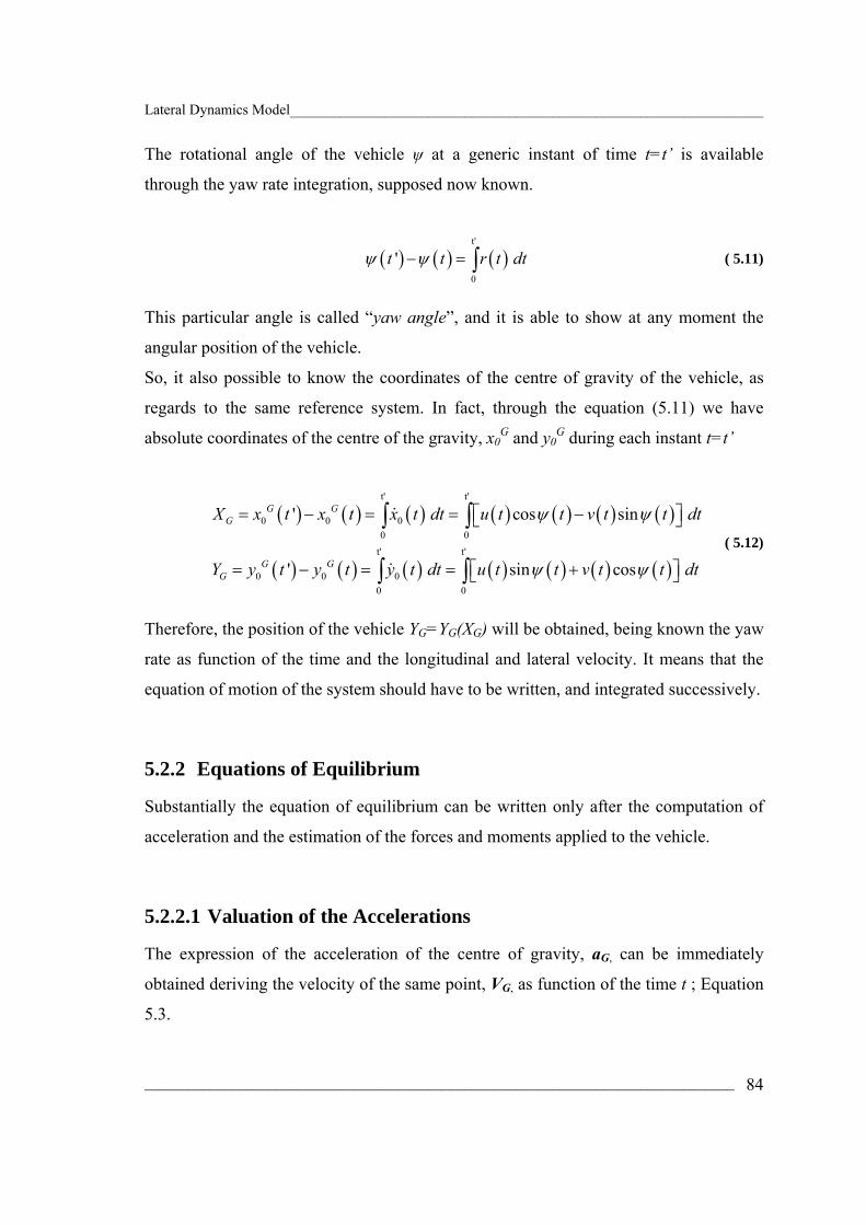
Lateral Dynamics Model_________________________________________________________________
_________________________________________________________________________________ 84
The rotational angle of the vehicle ψ at a generic instant of time t=t’ is available
through the yaw rate integration, supposed now known.
( ) ( ) ( )t'
0
' t t r t dtψ ψ− = ∫ ( 5.11)
This particular angle is called “yaw angle”, and it is able to show at any moment the
angular position of the vehicle.
So, it also possible to know the coordinates of the centre of gravity of the vehicle, as
regards to the same reference system. In fact, through the equation (5.11) we have
absolute coordinates of the centre of the gravity, x0G and y0
G during each instant t=t’
( ) ( ) ( ) ( ) ( ) ( ) ( )
( ) ( ) ( ) ( ) ( ) ( ) ( )
t' t'
0 0 00 0
t' t'
0 0 00 0
' cos sin
' sin cos
G GG
G GG
X x t x t x t dt u t t v t t dt
Y y t y t y t dt u t t v t t dt
ψ ψ
ψ ψ
= − = = −⎡ ⎤⎣ ⎦
= − = = +⎡ ⎤⎣ ⎦
∫ ∫
∫ ∫
&
&
( 5.12)
Therefore, the position of the vehicle YG=YG(XG) will be obtained, being known the yaw
rate as function of the time and the longitudinal and lateral velocity. It means that the
equation of motion of the system should have to be written, and integrated successively.
5.2.2 Equations of Equilibrium
Substantially the equation of equilibrium can be written only after the computation of
acceleration and the estimation of the forces and moments applied to the vehicle.
5.2.2.1 Valuation of the Accelerations
The expression of the acceleration of the centre of gravity, aG, can be immediately
obtained deriving the velocity of the same point, VG, as function of the time t ; Equation
5.3.

Lateral Dynamics Model_________________________________________________________________
_________________________________________________________________________________ 85
Figure 5.9: Trajectory of the Vehicle as regards to a Reference Coordinate System.
Obviously we must have into account that the versors i and j are changing direction
while the vehicle is moving through particular relations13:
( ) ( )
GG
Va i+ j+ j- i
- i+ j i+ j
x y
d u ur v vrdt
u vr v ura a
= =
= +
=
& &
& & ( 5.13)
Therefore, the acceleration of the centre of gravity has been broken up decomposed into
longitudinal and lateral directions:
-xa u vr= & ( 5.14)
and
ya v ur= +& ( 5.15)
13 The versors are a function of the time and so the derivate are developed: i jd r
dt= and
j id rdt
= − .

Lateral Dynamics Model_________________________________________________________________
_________________________________________________________________________________ 86
5.2.2.2 Forces and Moments
As known on a vehicle there are three kind of acting forces:
• force of gravity supposed acting in the centre of gravity;
• force of contact tyre-ground at four wheels;
• force of aerodynamics field due air resistent.
The external forces acting on the vehicle as a rigid body originate, at any moment, a
resultant force acting in a variable direction. In according to our fixed coordinate system
(x, y, z; G), it is defined with (X, Y, Z), the components of the resultant force totally
acting on the vehicle and with (L, M, N), its components of moments.
It is possible to write the equations of equilibrium, “Newton’s Laws” about the rigid
body which is moving in plane motion, having mass m and moment of inertia J, in Z-
axis direction.
Synthetically, the equations are developed into the following relations:
x
y
ma Xma Y
Jr Z
==
=& ( 5.16)
where X, Y and Z are the sum of longitudinal, transversal and rotational forces
respectively.
The most important forces acting on the vehicle are the traction forces tyre-ground,
shown in Figure 5.6. Strictly speaking, there are the aerodynamics resistent which is
proportional to the square velocity and the lateral force (for example exercised as
impulse by the wind).
In according to the conventions about the tyres, it is indicated with Fxij and Fyij the
longitudinal and lateral components of traction forces14 into point of contact tyre-
ground. Formally, in these forces Fxij and Fyij the traction and rolling forces are included
too.
14 The longitudinal and lateral forces Fxij and Fyij are denoted through the pedics i and j where the first describes the longitudinal or lateral direction and the second left or right wheels.

Lateral Dynamics Model_________________________________________________________________
_________________________________________________________________________________ 87
According to the working hypothesis about the steer angle, and particularly, for steer
angle in order to 15 degrees, we can linearize the equilibrium relationships. With
reference to Figure 5.10 the equilibrium equations are below shown:
( ) ( ) ( ) ( )( ) ( ) ( ) ( )
( ) ( ) ( )
( ) ( ) ( )
δ
δ
δ
δ δ
− = + − + + + −
+ = + + + + +
⎡ ⎤= + + + − + +⎣ ⎦
⎡ ⎤− − + − − +⎣ ⎦
&
&
&
11 12 11 12 21 22
11 12 11 12 21 22
11 12 11 12 1 21 22 2
11 12 21 22 11 12
2
x x y y x x xaero
x x y y y y
x x y y y y
x x x x y y
m u vr F F F F F F F
m v ur F F F F F F
Jr F F F F l F F l
tF F F F F F
( 5.17)
where Fxaero is the aerodynamics force15 applied by the air resistent:
ρ= 212xa xF SC u ( 5.18)
For the symmetry of the vehicle, it is suited to sum the contributions of the same axle to
have a compact notation, as shown into following relations:
= +
= +
= +
= +
1 11 12
2 21 22
1 11 12
2 21 22
x x x
x x x
y y y
y y y
F F FF F FF F F
F F F
( 5.19)
If it is taken into account that the traction torque is shared among two wheels at the
same axle by an ordinary differential (not auto-locked) it has another reduction in the
equations: =
=11 12
21 22
x x
x x
F FF F
( 5.20)
Even though there was a reduction into last equation of equilibrium there was always
the term (Fy11- Fy12)δ(t/2), but it is neglected for simplify.
15 The aerodynamic forces in lateral and vertical direction, Fyaero and Mzaero was neglected.

Lateral Dynamics Model_________________________________________________________________
_________________________________________________________________________________ 88
The interesting observation made about these relationships is that even if the wheels at
the same axle work with the same slip angle, the lateral forces at the same axle do not
have the same value. For this reason it is Fy11≠Fy12.
( )( )
δ
δ
δ
− = − + −
+ = + +
⎡ ⎤= + −⎣ ⎦
&
&
&
1 1 2
1 1 2
1 1 1 2 2
x y x xa
x y y
x y y
m u vr F F F F
m v ur F F F
Jr F F l F l
( 5.21)
which denotes the “Equation of Equilibrium”.
5.2.3 Constitutive Equations
To complete the vehicle dynamics modelling, we have to define the tyre behaviour at
each wheel. From a general point of view, the lateral forces Fyij are a function of slip
angle α, camber angle γ, longitudinal force Fxij and load transfer Fzij. Taking into
account only the functional variation about the slip angle, we will formulate the tyre
model able to integrate the equation of motion.
Figure 5.10: Forces Acting on the Vehicle

Lateral Dynamics Model_________________________________________________________________
_________________________________________________________________________________ 89
In the following section we again propose the linear tyre model. The most simplified
tyre model is a linear function, representing between the lateral force (or Cornering
Force) and the slip angle. This functional link is expressed into the following relation:
ij ijy ijF Cα α= ( 5.22)
where, being αi1=αi2, we have:
i iy iF Cα α= ( 5.23)
and Ci is the tyre cornering stiffness. The field working is characterized by small slip
angle, which means the order of magnitude is equal to 15÷20 degrees on dry road.
5.3 Single-Track Model
The most simplified vehicle dynamic model is a two/four-degree-of-freedom bicycle
model (or single track model), Figure 5.11, representing the lateral and yaw motions.
The mean idea behind this model is that in first approximation to develop lateral theory
it is not necessary or desirable to include the longitudinal direction, because we can
consider it known. This model, which is easier to understand than the others, is often
used in teaching purposes.
5.4 Two/Four-Degree-of-Freedom Vehicle Model Derivation
Capturing all the motions of a vehicle into analytical equations can be quite difficult.
Although including more number of elements in the model may increase the model’s
accuracy, it substantially increases the computation time. This section describes the
derivation of the two-degree-of-freedom bicycle model used in this study. It also
includes the equations for the front and rear tyre slip angles.

Lateral Dynamics Model_________________________________________________________________
_________________________________________________________________________________ 90
Figure 5.11: Reduction of Single Track Model.
5.5 Equations of Motion
Into the following section, the two degrees of freedom model considered for this study
is shown. Referring to Figure 5.12, the lateral and yawing velocities of the vehicle with
respect to the fixed coordinate system, XYZ can be described as shown in Equation 5.17
by the “equation of equilibrium”, below reported:
( )( )
δ
δ
δ
− = + − −
+ = + +
⎡ ⎤= + −⎣ ⎦
&
&
&
1 2 1
1 1 2
1 1 1 2 2
x x y xa
x y y
x y y
m u vr F F F F
m v ur F F F
Jr F F l F l
( 5.24)
and (5.10), “equations of congruence”:

Lateral Dynamics Model_________________________________________________________________
_________________________________________________________________________________ 91
1
2
f
r
v rlu
v rlu
α δ
α
+= −
−= −
( 5.25)
which includes the “constitutive equations”, referring to the tyre model, described
through one of these Equations 3.32, 3.34, and 3.43:
( )
1 exp
i i
i
y i
yi yi i p
yi yi zz
F C
d F F C Yu
Cd F F Fu F
α
α
α
α
α α
αµµ
=
+ = =
⎛ ⎞⎛ ⎞+ = − −⎜ ⎟⎜ ⎟⎜ ⎟⎝ ⎠⎝ ⎠
&
&
( 5.26)
where the subscript is i=f,r.
5.5.1 Rear Traction Model (RWD)
Further simplification about these equilibrium equations can be shown if we consider
the longitudinal velocity constant and the rear traction. In this case, the equations are
uncoupled and the first equation is algebraic one.
However, the mathematical problem is uncoupled only when the steer and traction have
been at different axis, but in this work it happens only in rear traction case. Also, the
longitudinal front force, Fxi, which includes only the rolling and the slope resistent,
could be neglected (Fx1=0).
To note that the longitudinal force, Fx2, does not appear into the equilibrium equations
even if it is the traction force applied by the tyre during the vehicle motion.

Lateral Dynamics Model_________________________________________________________________
_________________________________________________________________________________ 92
Figure 5.12: Single Track Model
5.5.1.1 Linear Tyre Model
Finally, the lateral dynamics system, 2 D.O.F. is described with only two differential
equations into variables v(t) and r(t).
α α α α α
α α α α α
δ
δ
+ + +⎛ ⎞ ⎛ ⎞= − − + +⎜ ⎟ ⎜ ⎟⎝ ⎠ ⎝ ⎠
⎛ ⎞− + +⎛ ⎞= − − +⎜ ⎟⎜ ⎟⎝ ⎠ ⎝ ⎠
&
&
1 2 1 1 2 2 1 1
2 21 1 2 2 1 1 2 2 1 1
1
x
x
C C C l C l C Fv v u rmu mu m
C l C l C l C l C Fr v r lJu Ju J
( 5.27)
These differential relations can be solved into analytical form too. During the following
paragraph we will show this kind of solution in comparison with the numerical form,
obtained by Matlab/Simulink software. Simply, the influence on the longitudinal force
Fxi can be neglected into the lateral problem, so the final equation of motion in rear
traction is:
α α α α α
α α α α α
δ
δ
+ +⎛ ⎞ ⎛ ⎞= − − + +⎜ ⎟ ⎜ ⎟⎝ ⎠ ⎝ ⎠
⎛ ⎞− +⎛ ⎞= − − +⎜ ⎟⎜ ⎟⎝ ⎠ ⎝ ⎠
&
&
1 2 1 1 2 2 1
2 21 1 2 2 1 1 2 2 1
1
C C C l C l Cv v u rmu mu m
C l C l C l C l Cr v r lJu Ju J
( 5.28)

Lateral Dynamics Model_________________________________________________________________
_________________________________________________________________________________ 93
5.5.1.1.1 Analytical Solution with Linear Tyre Model
To research the analytical solution, we had better have the state space representation of
the dynamic equations in (5.28) which is,
w=Aw+b& ( 5.29)
where, w(t)=(v(t),r(t)) is the state variables vector and the known term is given by
b(t)=(Cα1/m, Cα1l1/J)δ(t) and the matrix A is:
α α α α
α α α α
+ +⎡ ⎤+⎢ ⎥⎢ ⎥=
− +⎢ ⎥⎢ ⎥⎣ ⎦
1 2 1 1 2 2
2 21 1 2 2 1 1 2 2
A
C C C l C l umu mu
C l C l C l C lJu Ju
( 5.30)
One must note that the matrix A is a function of longitudinal velocity but not a steer
angle. The opposite case is vector b, which is a function of steering angle but not of a
longitudinal velocity.
The general solution of the equations of motion is a sum of a solution of associate
homogeneous problem and the solution of particular problem:
( ) ( ) ( )h pw t w t w t= + ( 5.31)
As known, the homogenous solution represents the transient history of the system,
instead the particular one the steady-state condition. Because the matrix A is not a
function of steer angle we can calculate the homogenous solution without fixed test of
simulation. In fact the first solution does not depend by the test simulation but the
second one can be valuated fixing the test of vehicle (for example “Steering Pad” and
“Lateral Impulse”).
The homogenous solution can be investigated imposing the known term vector as zero,
below shown:
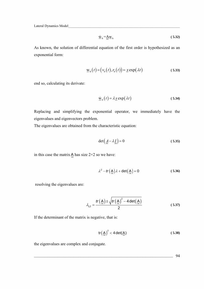
Lateral Dynamics Model_________________________________________________________________
_________________________________________________________________________________ 94
h hw =Aw& ( 5.32)
As known, the solution of differential equation of the first order is hypothesized as an
exponential form:
( ) ( ) ( )( ) ( )hw , exph ht v t r t x tλ= = ( 5.33)
end so, calculating its derivate:
( ) ( )hw expt x tλ λ=& ( 5.34)
Replacing and simplifying the exponential operator, we immediately have the
eigenvalues and eigenvectors problem.
The eigenvalues are obtained from the characteristic equation:
( )det 0A Iλ− = ( 5.35)
in this case the matrix A has size 2×2 so we have:
( ) ( )λ λ− + =2 A det A 0tr ( 5.36)
resolving the eigenvalues are:
( ) ( ) ( )λ
± −=
2
1,2
A A 4det A
2
tr tr ( 5.37)
If the determinant of the matrix is negative, that is:
( ) <2
tr A 4det(A) ( 5.38)
the eigenvalues are complex and conjugate.

Lateral Dynamics Model_________________________________________________________________
_________________________________________________________________________________ 95
In this case, developing both terms:
( ) α α α α⎡ ⎤+ += − + <⎢ ⎥
⎣ ⎦
2 21 2 1 1 2 21tr A 0C C C l C l
u m J ( 5.39)
and
( ) ( ) ( )α α α α⎡ ⎤= + − −⎣ ⎦
2 21 2 1 2 1 1 2 22
1det A C C l l mu C l C lu mJ
( 5.40)
These two quantities are very important concerning the eigenvalues:
( )( )
λ λ
λ λ
= +
=
1 2
1 2
A
det A
tr ( 5.41)
Obtained from the characteristic equation:
( )( )λ λ λ λ− − =1 2 0 ( 5.42)
Once known the eigenvalues, the eigenvectors are known too, through:
( ) 0i iA I xλ− = ( 5.43)
where i=1,2.
The particular solution of the dynamics system can be obtained fixing the test of
vehicle.
Assuming a “Steering pad” test (or “prova di colpo di sterzo”), [30, 31, 32, 33, 34, 35,
36], the particular solution is calculated from the system of equations:
pAw b− = ( 5.44)
and so:

Lateral Dynamics Model_________________________________________________________________
_________________________________________________________________________________ 96
( )( )
( )( )
( ) ( )
α α α α
α α α α
α α α α
α α α α
δ δ
δ δ
− −= =
− −
= =− −
2 22 2 1 1 2 2 1 1
2 221 2 1 1 2 2
1 2 1 22 22
1 2 1 1 2 2
det
det
p
p
C l l ml u C u C l l ml u C uv
C C l mu C l C lmJu A
C C lu C C lurC C l mu C l C lmJu A
( 5.45)
Once known vp and rp, lateral velocity and yaw rate in steady-state condition, it is
possible to calculate the “bend radius”, defined through the following relationship:
2
1 1 2 2
1 2
1 vp
p
C l C l m uuR lr C C l
α α
α αδ⎡ ⎤⎛ ⎞−
= = −⎢ ⎥⎜ ⎟⎝ ⎠⎣ ⎦
( 5.46)
where the value of rp was substituted. Using the definition of the slip angle at front and
rear wheels we have:
11
21
p pp
p pp
v r lu
v r lu
α δ
α
+= −
−= −
( 5.47)
and, immediately, the value of a characteristic velocity16 ut, which is illustrated for
completeness:
( ) ( ) ( )( )
2 22 21 2 1 1 2 2 1 2 1 2
21 1 2 2
4
4v v
tv
J C C m J C l C l m JC C l lu
m J C l C lα α α α α α
α α
⎡ ⎤+ + − − +⎣ ⎦=−
( 5.48)
Once known these variables, eigenvalues and eigenvectors are known and the solution,
consequently. In Appendix C, the Matlab m-file is illustrated.
5.5.1.1.2 Comparison between Analytical and Numerical Solution
In the following section the results concerning the analytical and numerical solution are
presented. The Runge-Kutta numerical method was used for the integration, with an 16 This velocity is defined as a particular velocity which defines a limited for the eigenvalue, changing from real and negative values to complex and conjugate.
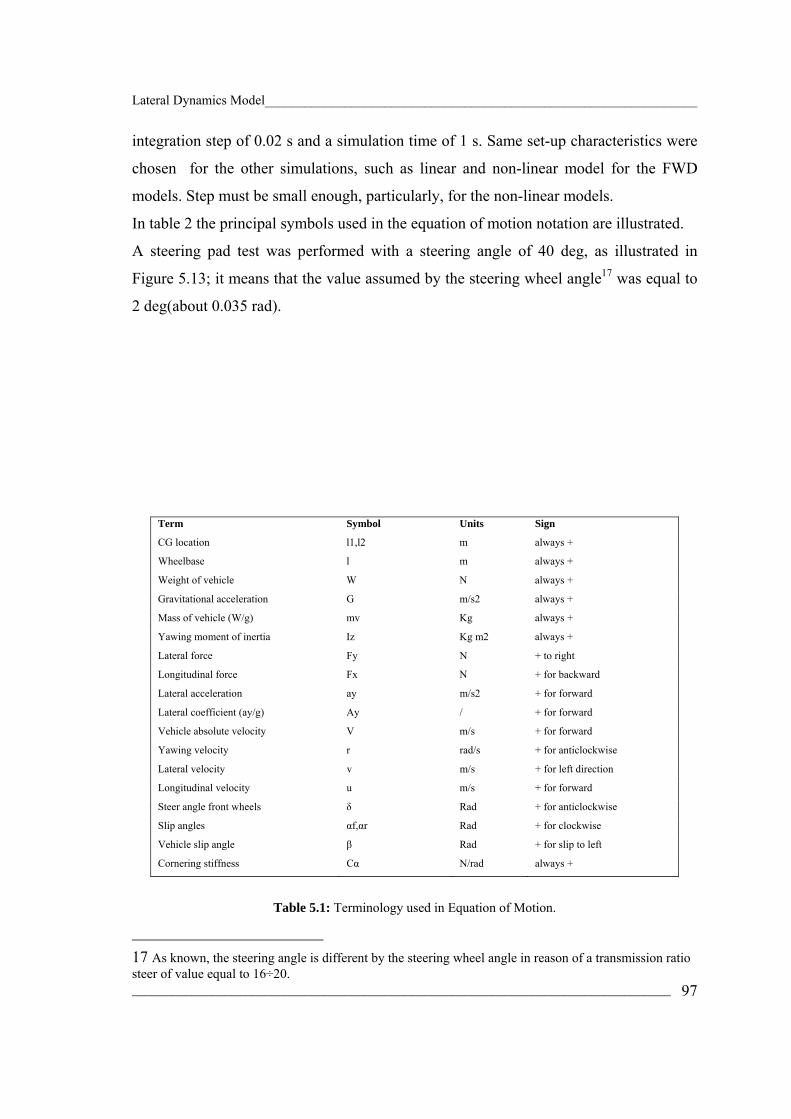
Lateral Dynamics Model_________________________________________________________________
_________________________________________________________________________________ 97
integration step of 0.02 s and a simulation time of 1 s. Same set-up characteristics were
chosen for the other simulations, such as linear and non-linear model for the FWD
models. Step must be small enough, particularly, for the non-linear models.
In table 2 the principal symbols used in the equation of motion notation are illustrated.
A steering pad test was performed with a steering angle of 40 deg, as illustrated in
Figure 5.13; it means that the value assumed by the steering wheel angle17 was equal to
2 deg(about 0.035 rad).
Term Symbol Units Sign
CG location l1,l2 m always +
Wheelbase l m always +
Weight of vehicle W N always +
Gravitational acceleration G m/s2 always +
Mass of vehicle (W/g) mv Kg always +
Yawing moment of inertia Iz Kg m2 always +
Lateral force Fy N + to right
Longitudinal force Fx N + for backward
Lateral acceleration ay m/s2 + for forward
Lateral coefficient (ay/g) Ay / + for forward
Vehicle absolute velocity V m/s + for forward
Yawing velocity r rad/s + for anticlockwise
Lateral velocity v m/s + for left direction
Longitudinal velocity u m/s + for forward
Steer angle front wheels δ Rad + for anticlockwise
Slip angles αf,αr Rad + for clockwise
Vehicle slip angle β Rad + for slip to left
Cornering stiffness Cα N/rad always +
Table 5.1: Terminology used in Equation of Motion.
17 As known, the steering angle is different by the steering wheel angle in reason of a transmission ratio steer of value equal to 16÷20.

Lateral Dynamics Model_________________________________________________________________
_________________________________________________________________________________ 98
0 0.1 0.2 0.3 0.4 0.5 0.6 0.7 0.8 0.9 10
5
10
15
20
25
30
35
40
Steering Angle-time cuve
[deg
]
time [s]
Figure 5.13: Steering Angle-time curve.
0 0.1 0.2 0.3 0.4 0.5 0.6 0.7 0.8 0.9 10
0.02
0.04
0.06
0.08
0.1
0.12
0.14
0.16
r [ra
d/s]
time [s]
Yawing Rate-time curve
r Analytical Solr Simulated
Figure 5.14: Yaw Rate-time curve.

Lateral Dynamics Model_________________________________________________________________
_________________________________________________________________________________ 99
0 0.1 0.2 0.3 0.4 0.5 0.6 0.7 0.8 0.9 1-0.08
-0.06
-0.04
-0.02
0
0.02
0.04
0.06
0.08
v [m
/s]
time [s]
Lateral Velocity-time curve
v Analytical Solv Simulated
Figure 5.15: Lateral Velocity-time curve.
0 0.1 0.2 0.3 0.4 0.5 0.6 0.7 0.8 0.9 12.2
2.3
2.4
2.5
2.6
2.7
2.8
2.9
3
Fy1
[kN
]
time [s]
Lateral Force front-time curve
Fy1 Analytical SolFy1 Simulated
Figure 5.16: Lateral Force Front-time
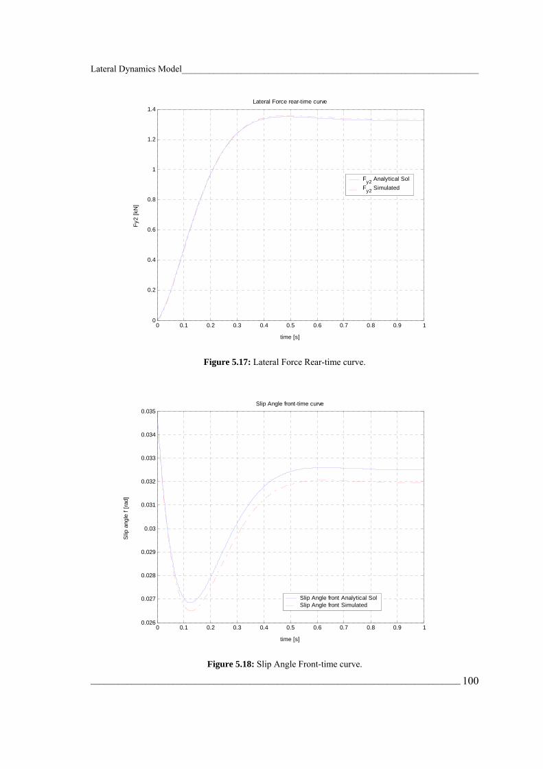
Lateral Dynamics Model_________________________________________________________________
_________________________________________________________________________________ 100
0 0.1 0.2 0.3 0.4 0.5 0.6 0.7 0.8 0.9 10
0.2
0.4
0.6
0.8
1
1.2
1.4
Fy2
[kN
]
time [s]
Lateral Force rear-time curve
Fy2 Analytical SolFy2 Simulated
Figure 5.17: Lateral Force Rear-time curve.
0 0.1 0.2 0.3 0.4 0.5 0.6 0.7 0.8 0.9 10.026
0.027
0.028
0.029
0.03
0.031
0.032
0.033
0.034
0.035
Slip
ang
le f
[rad]
time [s]
Slip Angle front-time curve
Slip Angle front Analytical SolSlip Angle front Simulated
Figure 5.18: Slip Angle Front-time curve.

Lateral Dynamics Model_________________________________________________________________
_________________________________________________________________________________ 101
0 0.1 0.2 0.3 0.4 0.5 0.6 0.7 0.8 0.9 10
0.002
0.004
0.006
0.008
0.01
0.012
0.014
0.016
0.018
Slip
Ang
le r
[rad]
time [s]
Slip Angle rear-time curve
Slip Angle rear Analytical SolSlip Angle rear Simulated
Figure 5.19: Slip Angle rear-time curve.
5.5.1.2 Linear Tyre Model with Relaxation Length
In the following treatment the equations for a single track model with linear tyre model
and relaxation length will be shown. One should note that in this case the degree of
freedom number of the system is changed. In fact, considering a linear tyre, the system
is a 2 D.O.F.s model, but taking into account a tyre model, traduced through a
differential equation, the new system will be defined as a 4 D.O.F.s model. In order to
develop this model completely, the equations (5.49) will be presented.
( )
α
α
δ
+ = +
= −
+⎛ ⎞+ = −⎜ ⎟⎝ ⎠
−⎛ ⎞+ = ⎜ ⎟⎝ ⎠
&
&
&
&
1 2
1 1 2 2
11 1
22 2
f
r
y y
y y
y y
y y
m v ur F F
Jr F l F l
v rld F F Cu u
rl vd F F Cu u
( 5.49)

Lateral Dynamics Model_________________________________________________________________
_________________________________________________________________________________ 102
5.5.1.3 Non-Linear Tyre Model with Relaxation Length
In analogy, it will be necessary to illustrate the equation of motion using the non-linear
tyre model. Likewise the former case, the model is a 4 D.O.F., too. The value of the
constants required for the integration are included as Appendix B.
( )
α
α
µ δµ
µµ
+ = +
= −
⎛ ⎞⎛ ⎞+⎛ ⎞+ = − − −⎜ ⎟⎜ ⎟⎜ ⎟⎜ ⎟⎝ ⎠⎝ ⎠⎝ ⎠⎛ ⎞⎛ ⎞−⎛ ⎞+ = −⎜ ⎟⎜ ⎟⎜ ⎟⎜ ⎟⎝ ⎠⎝ ⎠⎝ ⎠
&
&
&
&
1 2
1 1 2 2
11 1 1
1
22 2 2
2
1 exp
1 exp
y y
y y
fy y z
z
ry y z
z
m v ur F F
Jr F l F l
C v rld F F Fu F u
C v rld F F Fu F u
( 5.50)
5.5.1.3.1 Simulation Results
Simulation results for the first time are illustrated in Figures 5.20 to 5.25. Later than this
observation time all the working variables assume already a steady-state condition.
Moreover, the yaw rate is a increasing monotonic function and the lateral velocity
acquires a relative maximum in corresponding of 0.1 second and than it reaches the
steady-state condition.
Through the congruence equations, it is not hard to obtain the slip angles response.
However, it is possible to note the lateral forces at the front and rear wheels tendency.
In fact, owing to the steep steer angle, the front force in lateral direction assumes a
discontinuity about zero value. On the basis of that, the lateral front force does not start
from the zero value but from beginning it assumes a constant value, approximately
equal to the steady-state value.
This happens only for the linear tyre model without relaxation length, and Actually, for
this reason it is not able to describe the dynamic behaviour of the vehicle.

Lateral Dynamics Model_________________________________________________________________
_________________________________________________________________________________ 103
0 0.1 0.2 0.3 0.4 0.5 0.6 0.7 0.8 0.9 10
0.5
1
1.5
2
2.5
3
a y [m/s
2 ]
Time [s]
Lateral Acceleration-time curve
ay Linear modelay Linear Model with relaxation lengthay Non-Linear Model with relaxation length
Figure 5.20: Lateral Acceleration-time curve.
0 0.1 0.2 0.3 0.4 0.5 0.6 0.7 0.8 0.9 1-0.12
-0.1
-0.08
-0.06
-0.04
-0.02
0
0.02
0.04
0.06
0.08
v [m
/s]
Time [s]
Lateral Velocity-time curve
v Linear modelv Linear Model with relaxation lengthv Non-Linear Model with relaxation length
Figure 5.21: Lateral Velocity-time curve.

Lateral Dynamics Model_________________________________________________________________
_________________________________________________________________________________ 104
0 0.1 0.2 0.3 0.4 0.5 0.6 0.7 0.8 0.9 10
0.02
0.04
0.06
0.08
0.1
0.12
0.14
0.16
r [ra
d/s]
Time [s]
Yawing Rate-time curve
r Linear modelr Linear Model with relaxation lengthr Non-Linear Model with relaxation length
Figure 5.22: Yaw Rate-time curve.
0 0.1 0.2 0.3 0.4 0.5 0.6 0.7 0.8 0.9 10
0.5
1
1.5
2
2.5
3
Fy1[
kN]
Time [s]
Lateral Force front-time curve
Fy1 Linear modelFy1 Linear Model with relaxation lengthFy1 Non-Linear Model with relaxation length
Figure 5.23: Lateral Force Front-time curve.

Lateral Dynamics Model_________________________________________________________________
_________________________________________________________________________________ 105
0 0.1 0.2 0.3 0.4 0.5 0.6 0.7 0.8 0.9 10
0.2
0.4
0.6
0.8
1
1.2
1.4
Fy2
[kN
]
Time [s]
Lateral Force rear-time curve
Fy2 Linear modelFy2 Linear Model with relaxation lengthFy2 Non-Linear Model with relaxation length
Figure 5.24: Lateral Force Rear-time curve.
0 2 4 6 8 10 12 14 16 18 200
0.2
0.4
0.6
0.8
1
1.2
1.4Trajectory of the vehicle
Y [m
]
X [m]
Linear modelLinear Model with relaxation lengthNon-Linear Model with relaxation length
Figure 5.25: Trajectory of the Vehicle.
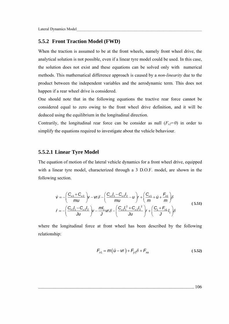
Lateral Dynamics Model_________________________________________________________________
_________________________________________________________________________________ 106
5.5.2 Front Traction Model (FWD)
When the traction is assumed to be at the front wheels, namely front wheel drive, the
analytical solution is not possible, even if a linear tyre model could be used. In this case,
the solution does not exist and these equations can be solved only with numerical
methods. This mathematical difference approach is caused by a non-linearity due to the
product between the independent variables and the aerodynamic term. This does not
happen if a rear wheel drive is considered.
One should note that in the following equations the tractive rear force cannot be
considered equal to zero owing to the front wheel drive definition, and it will be
deduced using the equilibrium in the longitudinal direction.
Contrarily, the longitudinal rear force can be consider as null (Fx2=0) in order to
simplify the equations required to investigate about the vehicle behaviour.
5.5.2.1 Linear Tyre Model
The equation of motion of the lateral vehicle dynamics for a front wheel drive, equipped
with a linear tyre model, characterized through a 3 D.O.F. model, are shown in the
following section.
α α α α α
α α α
δ δ
δ δ
+ −⎛ ⎞ ⎛ ⎞ ⎛ ⎞= − − − − + + +⎜ ⎟ ⎜ ⎟ ⎜ ⎟⎝ ⎠ ⎝ ⎠ ⎝ ⎠
⎛ ⎞− + +⎛ ⎞ ⎛ ⎞= − − − +⎜ ⎟ ⎜ ⎟⎜ ⎟⎝ ⎠⎝ ⎠ ⎝ ⎠
& &
&
1 2 1 1 2 2 1 1
2 21 1 2 2 1 1 2 21 1 1
1
x
V x
C C C l C l C Fv v vr u r umu mu m m
C l C l C l C lml C Fr v vr r lJu J Ju J
( 5.51)
where the longitudinal force at front wheel has been described by the following
relationship:
( ) δ= − + +&1 1x y xaF m u vr F F ( 5.52)

Lateral Dynamics Model_________________________________________________________________
_________________________________________________________________________________ 107
5.5.2.2 Linear Tyre Model with Relaxation Length
According to the corresponding model for the rear wheel drive, in this section it will be
illustrated the equations of motion for a 5 D.O.F.s model with front traction.
( )
α
α
δ
δ
δ
+ = + +
= − +
+⎛ ⎞+ = −⎜ ⎟⎝ ⎠
−⎛ ⎞+ = ⎜ ⎟⎝ ⎠
&
&
&
&
1 2 1
1 1 2 2 1 1
11 1
22 2
f
r
y y x
y y x
y y
y y
m v ur F F F
Jr F l F l F l
v rld F F Cu u
rl vd F F Cu u
( 5.53)
With the tractive front force Fx1 is expressed by the following relation, deduced by the
equilibrium in longitudinal direction; deduced by the longitudinal direction:
( ) δ= + + +&1 1x y xaF m u vr F F ( 5.54)
To note that in all equations concerning the FWD (each time the 1th of 5.24 was used),
the longitudinal acceleration was not simplified because the final purpose is to couple
the longitudinal and lateral models considering the variability longitudinal velocity.
Obviously, for fixed feed velocity, the value corresponding to the acceleration is null.
In the complete vehicle model, except the vertical dynamics, the tractive force will be
formed by more contributions, that during this section did not be consider, such as, the
rolling resistent which cannot simplified owing to the longitudinal velocity variability.
5.5.2.3 Non-Linear Tyre Model with Relaxation Length
In analogy to the former section, the front wheel drive model, 5 D.O.F. is traduced
through the following set of equations:

Lateral Dynamics Model_________________________________________________________________
_________________________________________________________________________________ 108
( )
α
α
δ
δ
µ δµ
µµ
+ = + +
= − +
⎛ ⎞⎛ ⎞+⎛ ⎞+ = − − −⎜ ⎟⎜ ⎟⎜ ⎟⎜ ⎟⎝ ⎠⎝ ⎠⎝ ⎠⎛ ⎞⎛ ⎞−⎛ ⎞+ = −⎜ ⎟⎜ ⎟⎜ ⎟⎜ ⎟⎝ ⎠⎝ ⎠⎝ ⎠
&
&
&
&
1 2 1
1 1 2 2 1 1
11 1 1
1
22 2 2
2
1 exp
1 exp
y y x
y y x
fy y z
z
ry y z
z
m v ur F F F
Jr F l F l F l
C v rld F F Fu F u
C v rld F F Fu F u
( 5.55)
where Fx1 assumes the same form used in the linear front model with the relaxation
length, Eqs. (5.45).According to the former treatment about the simulations shown, the
front wheel drive model response will be proposed, with three different tyre models,
before analyzed, Figures 5.26 to 5.31.
0 0.1 0.2 0.3 0.4 0.5 0.6 0.7 0.8 0.9 10
0.5
1
1.5
2
2.5
3
3.5
4Lateral Acceleration-time curve
time [s]
a y [m/s
2 ]
Linear modelLinear model with relaxation legthNon-Linear model with relaxation legth
Figure 5.26: Lateral Acceleration-time curve.

Lateral Dynamics Model_________________________________________________________________
_________________________________________________________________________________ 109
0 0.1 0.2 0.3 0.4 0.5 0.6 0.7 0.8 0.9 1-0.2
-0.15
-0.1
-0.05
0
0.05
0.1
0.15
v [m
/s]
Time [s]
Lateral Velocity-time curve
v Linear modelv Linear Model with relaxation lengthv Non-Linear Model with relaxation length
Figure 5.27: Lateral Velocity-time curve.
0 0.1 0.2 0.3 0.4 0.5 0.6 0.7 0.8 0.9 10
0.02
0.04
0.06
0.08
0.1
0.12
0.14
0.16
0.18
r [ra
d/s]
Time [s]
Yawing Rate-time curve
r Linear modelr Linear model with relaxation lengthr Non-Linear model with relaxation length
Figure 5.28: Yaw Rate-time curve.

Lateral Dynamics Model_________________________________________________________________
_________________________________________________________________________________ 110
0 0.1 0.2 0.3 0.4 0.5 0.6 0.7 0.8 0.9 10
0.5
1
1.5
2
2.5
3
Fy1
[kN
]
Time [s]
Lateral Force front-time curve
Fy1 Linear modelFy1 Linear model with relaxation lengthFy1 Non-Linear model with relaxation length
Figure 5.29: Lateral Force Front-time curve.
0 0.1 0.2 0.3 0.4 0.5 0.6 0.7 0.8 0.9 10
0.2
0.4
0.6
0.8
1
1.2
1.4
Fy2
[kN
]
Time [s]
Lateral Force rear-time curve
Fy2 Linear modelFy2 Linear model with relaxation lengthFy2 Non-Linear model with relaxation length
Figure 5.30: Lateral Force Rear-time curve.

Lateral Dynamics Model_________________________________________________________________
_________________________________________________________________________________ 111
0 2 4 6 8 10 12 14 16 18 200
0.2
0.4
0.6
0.8
1
1.2
1.4Trajectory of the vehicle
Y [m
]
X [m]
Linear modelLinear model with relaxation lengthNon-Linear model with relaxation length
Figure 5.31: Trajectory of the Vehicle.
5.5.3 Conclusions
Schematically, the models developed in this section can be summarized in a single
table; see Table 5.2.
Degrees of Freedom Tyre Model
2 L 4 L with R-L
RWD 4 N-L with R-l
3 L
5 L with R-L
FWD 5 N-L with R-l
Table 5.2: Degrees of Freedom Corresponding to each Lateral Model

Lateral Dynamics Model_________________________________________________________________
_________________________________________________________________________________ 112
The mean of the symbols is reported in the following sentences:
• L: Linear tyre model without relaxation length;
• L with R-L: Linear tyre model with relaxation length
• N-L with R-L: Non-Linear tyre model with relaxation length
• RWD: Rear wheel drive;
• FWD: Front wheel drive.
To note that, for the vehicle complete model, so with the interaction between the
longitudinal and lateral variables, each model will acquire one degree of freedom
considering a linear tyre model with/without relaxation length and three degrees fo
freedom considering the non-linear tyre model. Schematically these concepts are
illustrated in the following table:
Longitudinal Model
(D.O.F.s) Lateral Model
(D.O.F.s) Degree of Freedom
1 2 3 1 4 5
RWD 3 4 7
1 3 4
1 5 6
FWD 3 5 8
Table 5.3: Degrees of Freedom Corresponding to each Complete Model

_________________________________________________________________________________ 113
Chapter 6
6 Simulink Environment Model
As described into the former chapters, numerous equations are required to develop a
complete vehicle model and study the principal characteristics about vehicle dynamics.
Obviously, the decision about how to go into details rests entyrely on the discretion of
the research worker. In fact, it always happens that the choice about the details is
imposed due to the final goal of the research, and for this reason, one does not need to
model the complete physical system, only part of it. In this section we will introduce the
simple model, previously discussed, in order to give a complete vision about the
principal characteristics of longitudinal and transversal behaviour of the vehicle. Thus,
the general characteristics of vehicle, will be implemented in Simulink/Matlab
environment.
6.1 Simulink Modelling
In order to analyze the dynamic characteristics of the vehicle and to study its
performance, a computer simulation model of the vehicle system, using the
Matlab/Simulink computer software, has been developed.
In fact, this section describes the Matlab/Simulink model that was implemented.
Simulink is a software package for modelling, simulating, and analyzing dynamical
systems in general.

Simulink Environment Model____________________________________________________________
_________________________________________________________________________________ 114
The software, implemented runs under Matlab, a mathematical workshop. Simulink and
Matlab are available from the MathWorks, Inc. Simulink provides a graphical user
interface for building models as block diagrams.
The graphical interface is popular for developing dynamical models for many fields,
such as electronics, hydraulics, chemistry, and many others.
Simulink is not particularly useful for building equation sets for complex mechanical
3D systems. However, it includes S-functions (system functions) to augment and extend
the building blocks in SIMULINK to include arbitrary complex systems.
The S-function appears in a SIMULINK model as a block in the block diagram. The
mathematical behaviour of S-functions can be defined either as a MATLAB M-file, or
as an executable piece of object code in the form of a DLL (dynamic link library)
obtained by compiling C or FORTRAN source code. Such “executable” functions are
called MEX files (where the EX stands for executable). The S-functions can be loaded
and run by SIMULINK. The simulations can be run from within SIMULINK, using the
SIMULINK integrators and the SIMULINK environment for setting control inputs to
the vehicle model.
6.2 Simulating a Complete Vehicle
The simulation model, illustrated in Figure 6.1, includes many sub-models, some of that
will simulate the powertrain, other the lateral motion of the vehicle, and others the tyre
behaviour.
The green and yellow blocks on the right, named “Vehicle Dynamics” and “Tyre
Model” represent the final part of the vehicle modelling: the dynamics behaviour of the
chassis, vehicle inertia, the wheels, and their coupling to the road.
All the other subsystems in the model represent input that control the former or outputs
that measure its behaviour.
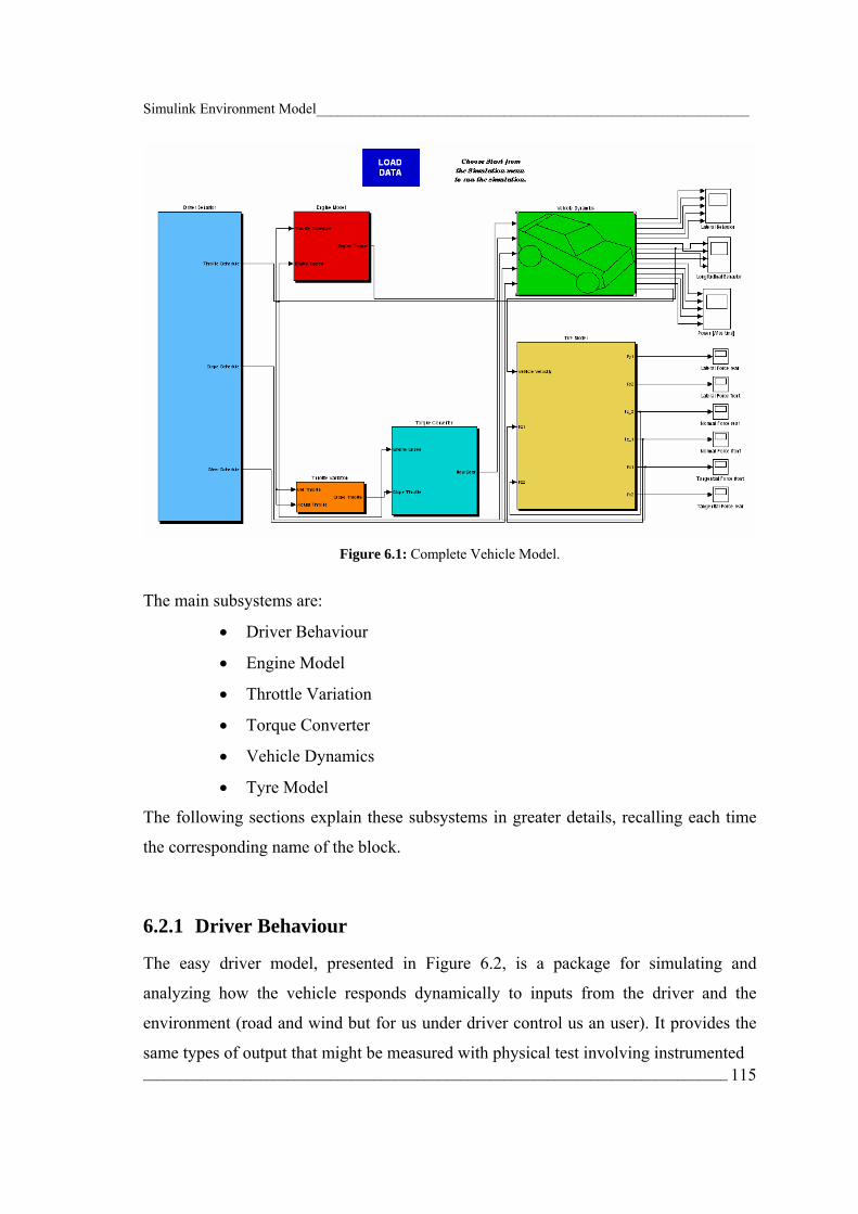
Simulink Environment Model____________________________________________________________
_________________________________________________________________________________ 115
Figure 6.1: Complete Vehicle Model.
The main subsystems are:
• Driver Behaviour
• Engine Model
• Throttle Variation
• Torque Converter
• Vehicle Dynamics
• Tyre Model
The following sections explain these subsystems in greater details, recalling each time
the corresponding name of the block.
6.2.1 Driver Behaviour
The easy driver model, presented in Figure 6.2, is a package for simulating and
analyzing how the vehicle responds dynamically to inputs from the driver and the
environment (road and wind but for us under driver control us an user). It provides the
same types of output that might be measured with physical test involving instrumented

Simulink Environment Model____________________________________________________________
_________________________________________________________________________________ 116
Figure 6.2: Driver Behaviour Block
vehicles (as will be the case for the validation test). The aim of this section is to provide
information on the technical aspects of the simulations.
6.2.2 Powertrain Modelling
As cited into Chapter 4, modelling the powertrain requires good knowledge of the
involved components and their physic. It is remembered the division modelling into
three parts, Engine Model and Throttle Variation Model and Torque Converter Model,
including torque converter model.
6.2.2.1 Engine Model
The characteristic curve of an internal combustion engine defines the torque supplied as
function of engine speed ne and throttle opening α. The former is regulated by the driver
behaviour model, assuming values between zero and one.
The Simulink block “Engine Model”, first element of the complete vehicle model is
shown in Figure 6.3. It should be noted that this block is called MISO (Multi-Input-
Single-Output) because, during the simulation, for a fixed value of the engine speed and
throttle opening, it gives the value of the corresponding engine torque.
Figure 6.3: Engine Model.

Simulink Environment Model____________________________________________________________
_________________________________________________________________________________ 117
From this, we obtain the subsystem shown in Figure 6.4. In this former block a “Look
up table 2D” was used. It gives the interpolation points in the engine map; so, Tables
6.1, and 6.2 show the functional description of this block.
Figure 6.4: Subsystem Corresponding to the Engine Model.
Input Description Size Units
Throttle
Schedule Matrix value assumed by the driver tout× 1 %
Engine Speed Instantaneous value assumed by the engine
speed tout× 1 rpm
Table 6.1: Input of the Engine Model.
Output Description Size
Engine Torque Engine torque value of needed to integrate
the state equation tout× 1
Table 6.2: Output of the Engine Model.
6.2.2.2 Throttle Variation Model
The next subsystem in the powertrain is the driveline, in this case an automated manual
transmission, driveshaft, wheels and chassis. Actually, the transmission has three
working states: engaged, disengaged and during engagement/disengagement.
When the transmission is engaged the engine power is transferred to the wheels via a
fixed gear ratio. On the other hand, when the transmission is de-coupled the rotational
parts in engine run without transferring tractive effort to the wheels.
In this work, we have designed a simple Torque Converter model to simulate the gear
change, as shown in Table 6.3:

Simulink Environment Model____________________________________________________________
_________________________________________________________________________________ 118
Acceleration Deceleration
1-2 5-4
2-3 4-3
3-4 3-2
4-5 2-1
Steady speed Arrest
Table 6.3: Gear Change during Acceleration and Deceleration Manoeuvreing.
Before describing this subsystem accurately, we have to understand which
manoeuvreing we are using. To do this, we need a special block, called “Throttle
Variation”, shown in Figure 6.5.
In following Tables 6.4, 6.5, and 6.6 we have the functional description, with reference
to the Function Fcn(u), Derivate Computation, where tout assumes values depending on
the simulation time.
Figure 6.5: Throttle Variation Model.
Also, we will illustrate the corresponding subsystem of this model, as shown in Figure
6.5.
Figure 6.6: Subsystem corresponding to the Throttle Variation Model.

Simulink Environment Model____________________________________________________________
_________________________________________________________________________________ 119
Input Description Size Units
Old Throttle Old Value assumed by Throttle tout×1 /
Actual Throttle Actual Value assumed by Throttle tout×1 /
Table 6.4: Input of the Throttle Variation Model
Function Description Size
F(u)
Evaluate the numerical derivate between
Actual and Old Throttle
/
Table 6.5: Fcn-Function of the Throttle Variation Model
Output Description Size
Slope Throttle Variable needed to simulate the gear-change
manoeuvreing tout× 1
Table 6.6: Output of the Throttle Variation Model Depending on the value assumed by Slope Throttle, it should have the corresponding
gear change. This logic disposition is dictated from the S-Function,
“gear_box_change”, included in Torque Converter model, explained into section.
6.2.2.3 Torque Converter Model
As mentioned previously, the power-torque-speed characteristics of the internal
combustion engine are not suited for direct vehicle propulsion. Transmission, therefore,
is required to provide the vehicle with tractive effort speed characteristics that will
satisfy the load demands under various operating conditions.
The term “transmission” includes all the systems or subsystems used for transmitting
the engine power to the driven wheels or sprockets. There are two common types of
transmission with a torque converter: the manual gear transmission, and the automatic
transmission with a torque converter. Other types of transmission such as the continuous
variable transmission (CVT) and the hydrostatic transmission are also used.

Simulink Environment Model____________________________________________________________
_________________________________________________________________________________ 120
In this project, an automatic transmission is simulated, according to two limit values of
engine speed. These two limits are imposed arbitrarily setting a range between
maximum and minimum number of revolutions. In this case, the higher limit to change-
up gear (acceleration) is 5000 rpm and the lower one to change-down gear
(deceleration) is 2000 rpm.
The “Torque Converter” model, shown in Figure 6.7, works according to an S-Function,
called “gear_box_change”, and are included in Appendix B.
In the following Tables 6.7, 6.8, and 6.9 a description functionally was shown.
Therefore, the corresponding subsystem of this model is illustrated in Figure 6.8.
Figure 6.7: Torque Converter Model
Figure 6.8: Subsystem Corresponding to the Torque Converter Model

Simulink Environment Model____________________________________________________________
_________________________________________________________________________________ 121
However, as shown in the previous subsystem, we have two main parts: the Switch
block and Gear Selector block. The first one is indispensable to give the initial
condition corresponding to start in 1st gear. On the other hand, the other block recalls
the S-Function, as shown in Figure 6.8.
Figure 6.9: Subsystem Corresponding to the Gear Selector Block
Input Description Size Units
Slope Throttle Slope Value assumed by Throttle tout×1 /
Engine Speed Instantaneous value assumed by Engine
Speed tout×1 /
Table 6.7: Input of the Torque Converter Model
Function Description Size
F(u)
Valuate the new gear number
/
Table 6.8: S-Function of the Torque Converter Model
Output Description Size
New Gear Value of new gear number tout×1
Table 6.9: Output of the Torque Converter Model

Simulink Environment Model____________________________________________________________
_________________________________________________________________________________ 122
6.2.3 Vehicle Dynamics
The Vehicle Dynamics model, Figure 6.10, is divided into two parts:
• Driveline Model;
• Lateral Model.
In the following sections, all the subsystems will be illustrated.
Figure 6.10: Vehicle Dynamics.
6.2.3.1 Driveline Model
This easy model can be considered as the latter link of the chain, namely Longitudinal
Vehicle Dynamics.
The equation of motion is a function of time-varying quantities that characteristic curve
of an internal combustion engine defines the torque supplied as function of engine speed
ne and throttle opening α that is as function of a parameter able to show how much the
throttle should be opened. In fact, as known, the throttle opening is proportional to the
mass flow rate of air.
The throttle opening assumes included values between 0, section completely closed and
1 (or percentage value) for fully opening.
Particularly attention may be given to the Memory block, Figure 6.22, which contains
the condition concerning the velocity of the wheels constant during the gear-change
manoeuvreing. In fact, during an unitary step of simulation, when the gear has engaged
the simulation is stopped artificially and the rotational velocity of the wheels is imposed
to be constant. All these manoeuvreings are controlled by the variable “trigger”, which

Simulink Environment Model____________________________________________________________
_________________________________________________________________________________ 123
gives the null value, when the gear number is constant, and unitary value during the
change-gear. To have the graphical visualization see Figure 6.17.
Figure 6.11: Driveline Model.
Figure 6.12: Driveline Subsystem.
Figure 6.13: Aerodynamic Block.

Simulink Environment Model____________________________________________________________
_________________________________________________________________________________ 124
Figure 6.14: Rolling Torque Block.
Figure 6.15: Grade Torque Block.
Figure 6.16: Inertia Evaluation Block.

Simulink Environment Model____________________________________________________________
_________________________________________________________________________________ 125
Figure 6.17: Trigger Block.
Figure 6.18: Wheel Shaft Block 1
Figure 6.19: Wheel Shaft Block 2
Figure 6.20: Wheel Shaft Subsystem 1

Simulink Environment Model____________________________________________________________
_________________________________________________________________________________ 126
Figure 6.21: Wheel Shaft Subsystem 2
Figure 6.22: Memory Block
6.2.3.2 Lateral Model
In following section the lateral dynamics system (only FWD one) in Matlab/Simulink
environment will be illustrated.
Figure 6.23: FWD Lateral Model Block

Simulink Environment Model____________________________________________________________
_________________________________________________________________________________ 127
Figure 6.24: FWD Lateral Model Subsystem Block
Figure 6.25: Lateral Model y Subsystem Block

Simulink Environment Model____________________________________________________________
_________________________________________________________________________________ 128
Figure 6.26: Lateral Model r Subsystem Block
Figure 6.27: Lateral Acceleration Subsystem Block
Figure 6.28: Trajectory Subsystem Block
6.2.4 Tyre Model
In order to have more simplicity the tyre model is subdivided into two parts:
• Longitudinal and normal behaviour;
• Lateral behaviour.

Simulink Environment Model____________________________________________________________
_________________________________________________________________________________ 129
Therefore, the blocks are shown separately, dividend the normal and longitudinal forces
at the wheels and the lateral ones. One can note that changing the tyre model concerning
the lateral behaviour, the longitudinal and normal behaviour does not change.
Figure 6.29: Tyre Model.
6.2.4.1 Normal and Longitudinal Behaviour
In the following section, the former one is illustrated; see Figures 6.30, 6.31, 6.32,
6.322, 6.34, and 6.35.
Figure 6.30: Normal and Longitudinal Behaviour (Tyre Model).

Simulink Environment Model____________________________________________________________
_________________________________________________________________________________ 130
Figure 6.31: Normal and Longitudinal Behaviour Subsystem.
Figure 6.32: Normal rear Force Sub-Model (Tyre Model).

Simulink Environment Model____________________________________________________________
_________________________________________________________________________________ 131
Figure 6.33: Normal front Force Sub-Model (Tyre Model).
Figure 6.34: Longitudinal front Force Sub-Model (Tyre Model).
Figure 6.35: Longitudinal rear Force sub-Model (Tyre Model).
6.2.4.2 Lateral Behaviour
In analogy the lateral behaviour is configured as shown in Figures 6.36 and 6.37.

Simulink Environment Model____________________________________________________________
_________________________________________________________________________________ 132
Figure 6.36: Lateral Behaviour (Tyre Model).
Figure 6.37: Lateral Front and Rear Forces subsystem (Tyre Model).
6.2.5 Real time Simulator Block
The Vehicle Driving Simulator is a simple sub-model implemented in the Driver-Block.
It is only an “physical” interface between the human driver and the vehicle complete
model.

Simulink Environment Model____________________________________________________________
_________________________________________________________________________________ 133
From now on the VDS block was running on a 1.39 GHz AMD Atlon-based computer
while the driving scene was presented on a 15-inch monitor. A more powerful computer
could be useful in order to simulate the behaviour of the model not in “real time”,
without delays due to the complete integration of the mathematical equations.
The physical configuration of the simulator consist of:
• Seat
• Steer system
• Monitor
• Accelerator and brake pedal (the latter is not used)
The whole elements, shown in Figure 6.37, such as the steer and accelerator pedal have
been added to the PC to reproduced with startling realism the physical environment of a
typical vehicle.
The VDS simulator software is configured to represent the control/response
characteristics typical of a real vehicle. In fact, step for step the differential equations of
motion were integrating.
Obviously, the graphical aspect was take into account. The vehicle was represented by a
single point and the trajectory was just a single line.
Even so the model represents with good approximation the real system, according to the
whole hypothesis made.
Figure 6.38: Elements of the Vehicle Simulator
The bock used to link the human driver to the Simulink/Matlab model is a Virtual
Reality Toolbox, as shown in Figure 6.38.

Simulink Environment Model____________________________________________________________
_________________________________________________________________________________ 134
Figure 6.39: VDS Simulator block
_________________________________________________________________________________ 135
Chapter 7
7 Validation of the Vehicle Model
Once the model is constructed it must be verified with as much information from the
real system as possible. This process is known as “validation”. The most common
method to evaluate the reaction of the model to measured data and compare it with
actual values. For this reason, this chapter begins with our approach to the validation of
the model and all connected problems concerning the measure errors. In the foregoing
chapters, we used a simplified mathematical model of the complete vehicle to develop
some basic concepts, and then we conclude with test results on real vehicles.
7.1 The Simulation of the Systems
The simulation is a method used to verify a model which represents the behaviour of a
physical system. Therefore, a validation phase is required, during which the results of
the model will come compared with the experimental data.
As described into Chapter 2, the simulators are much utilized in all industrial fields such
as aero spatial, aeronautic, motor and many others, in order to understand the physical
behaviour of a system. In some applications user is constrained to work with a simulator
model, because there is no other way to study the phenomenon, such as the evolution of
the universe, the meteorological and seismic ones.

Validation of the Vehicle Model___________________________________________________________
_________________________________________________________________________________ 136
The results obtained by the simulations, such as the tendency of the variables, can be
visualized graphically, by animation software (2D or 3D), in order to represents the
evolution of the system during the time.
7.2 Validation Procedure
The construction of a model often involves many simplifications through which the
outputs of the model deviate to a greater or lesser extent from the real values. Before
proceeding to the real validation, some responses could be interesting, to understand
completely the following development:
• Do the model outputs correspond well enough to the measured data?
• Is the model suitable for the purpose for which it was constructed?
The more data are available from the real system, the better the above questions can be
responded. A model can in general be considered validated when, following evaluation
with suitable validation data, it satisfies the requirements for which it was constructed.
Before the validation, one must clearly know which purpose the model is to be put to,
which outputs must be precisely modeled, and where certain errors can be accepted.
Once the model will result “true” we will be arrived to the last stage of the modelling.
Opposite a cut-off stage for the model will be required.
Generally, the principle of validation of the model consists to compare the output
variables of the model with the estimations measured experimentally. Initially, to do
this, it is necessary to fix rich input variables and so to realize a test protocol. The
principal aim of the test execution is the acquisition of the data, which will come used to
validate the model.
Some sensors will have to fix on the working system in order to measure the physical
variables. These variables will be subject to measurement errors and, for this reason, it
will be necessary an arrangement stage.
7.2.1 Definition of a Test Protocol
To realize the validation of a model, the choice about the working signal is very
important. It is necessary that these signals should have much information in order to

Validation of the Vehicle Model___________________________________________________________
_________________________________________________________________________________ 137
investigate on a large functioning field of the vehicle. For this reason, the working
signal must be continuous. Generally, the ideal signal to validate all the models is the
white noise.
Unluckily, this kind of signal often is not available. The binary signal which has similar
characteristics to the white noise is available. This kind of signal is a deterministic one
with a rich frequency band.
The different signals used will have to allow the validation of the model in all working
regimes, transient or steady-state. The choice about the working signals influence the
tests made. The definition of the test protocol is very important to validate the
mathematical model. It allows realizing the suitable tests that we have to analyze.
In the literature many norms (ISO), [30, 31, 32, 33, 34, 35, 36] are available for
different applications. In the section 7.2.5, the discussion about the tests used for our
application will be shown.
The description of the norms ISO presents a particular structure constituted by different
specifications:
• Application data;
• Instrumentation (standard or special);
• Installation of the sensors;
• Tests conditions;
• Analysis and presentation of the tests.
All this information will have to be planned during the time, in order to understand what
we have to do before, during and after the tests. The basis notions, which have to be
respectful, are described in the theory about the experience plane [37, 38].
7.2.2 Data Acquisition. Measures
Before making all the tests, one should question oneself about the variables to be
measured for the current application. Obviously, the choice about the measure variables
influences the typology of the mechanical sensors, but the latter are only a link of the
complete measure chain, as shown in Figure 7.1.
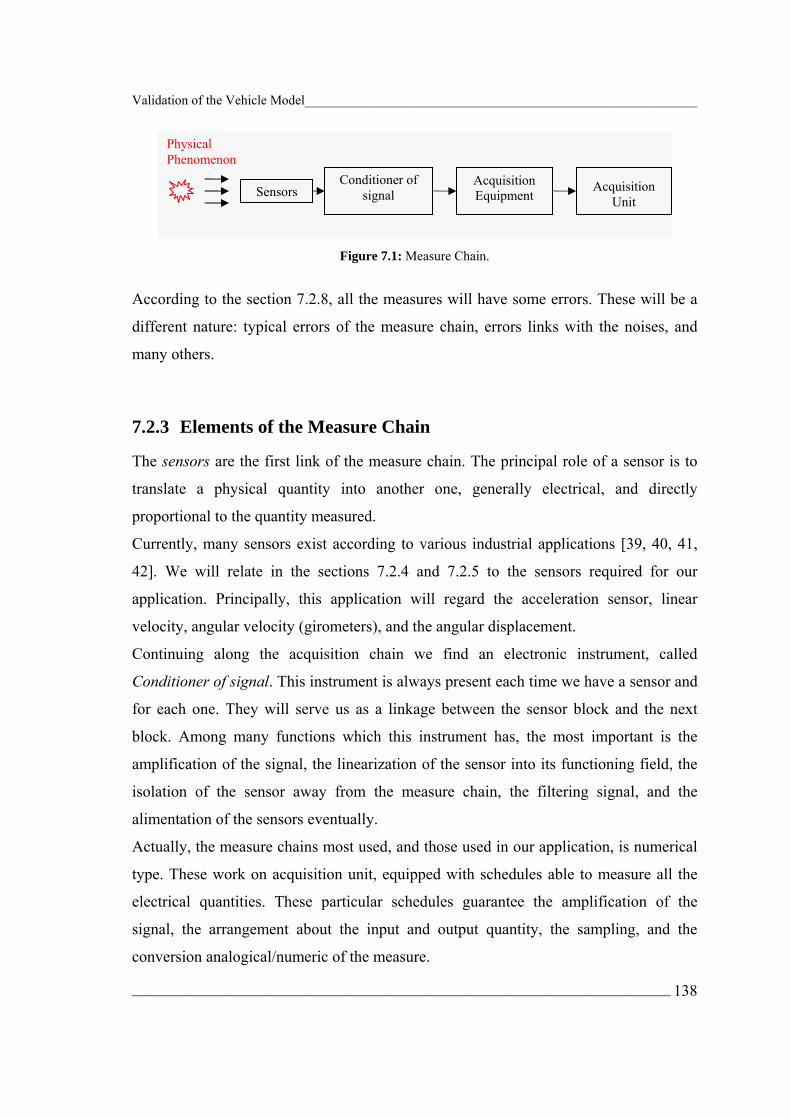
Validation of the Vehicle Model___________________________________________________________
_________________________________________________________________________________ 138
Figure 7.1: Measure Chain.
According to the section 7.2.8, all the measures will have some errors. These will be a
different nature: typical errors of the measure chain, errors links with the noises, and
many others.
7.2.3 Elements of the Measure Chain
The sensors are the first link of the measure chain. The principal role of a sensor is to
translate a physical quantity into another one, generally electrical, and directly
proportional to the quantity measured.
Currently, many sensors exist according to various industrial applications [39, 40, 41,
42]. We will relate in the sections 7.2.4 and 7.2.5 to the sensors required for our
application. Principally, this application will regard the acceleration sensor, linear
velocity, angular velocity (girometers), and the angular displacement.
Continuing along the acquisition chain we find an electronic instrument, called
Conditioner of signal. This instrument is always present each time we have a sensor and
for each one. They will serve us as a linkage between the sensor block and the next
block. Among many functions which this instrument has, the most important is the
amplification of the signal, the linearization of the sensor into its functioning field, the
isolation of the sensor away from the measure chain, the filtering signal, and the
alimentation of the sensors eventually.
Actually, the measure chains most used, and those used in our application, is numerical
type. These work on acquisition unit, equipped with schedules able to measure all the
electrical quantities. These particular schedules guarantee the amplification of the
signal, the arrangement about the input and output quantity, the sampling, and the
conversion analogical/numeric of the measure.
Sensors Conditioner of
signal
Acquisition Unit
Acquisition Equipment
Physical Phenomenon

Validation of the Vehicle Model___________________________________________________________
_________________________________________________________________________________ 139
The acquisition unit serves to manipulate all the measure chain from a PC in order to
store the acquired data on a memory support. Finally, the software is able to pilot the
acquisition chain according with specified rules. The last element of the measure chain
is the connection between the different elements with the cables. This aspect is very
important because it could verify same disturbances on account of interferences.
Today the multiplication technique is used frequently. This kind of connection is able to
link many blocks with only one common cable. Particularly, for this application the
CAN control Area Network has been used. In this way the wiring is reduced to the
minimum.
7.2.4 Tests and Measurements
To validate a mathematical model, an experimental stage is required in order to evaluate
all variables. Therefore, these will have to be compared with the estimates of our model.
In our case, some tests on a track have been performed with a suitably-equipped test
vehicle.
Previously, we needed to decide the necessary instruments, such as the sensors, the
acquisition system and all the components for the measure chain.First, for a good
validation of our models, we need to choose correct practice signals to supply the large
functioning of the vehicle. Therefore, we are required to define a test protocol which
explains the dynamic manoeuvreing in terms of external conditions and other factors.
Finally, the results obtained will be manipulated to develop their own meaning.
7.2.5 Instrumentation of Vehicle
To study the dynamics problems, shown in previous chapters, it was decided to use, like
the test vehicle, Renault Mégane Coupé 16V 150 hp equipped with different sensors
and an acquisition system AUTOBOX; see Figure 7.2.
To validate the mathematical model, tests on a track have been performed with a
suitably-equipped test vehicle. Thus, prior to this study, the necessary instrumentation
as well as the acquisition system had to be defined. A particular study on the excitation
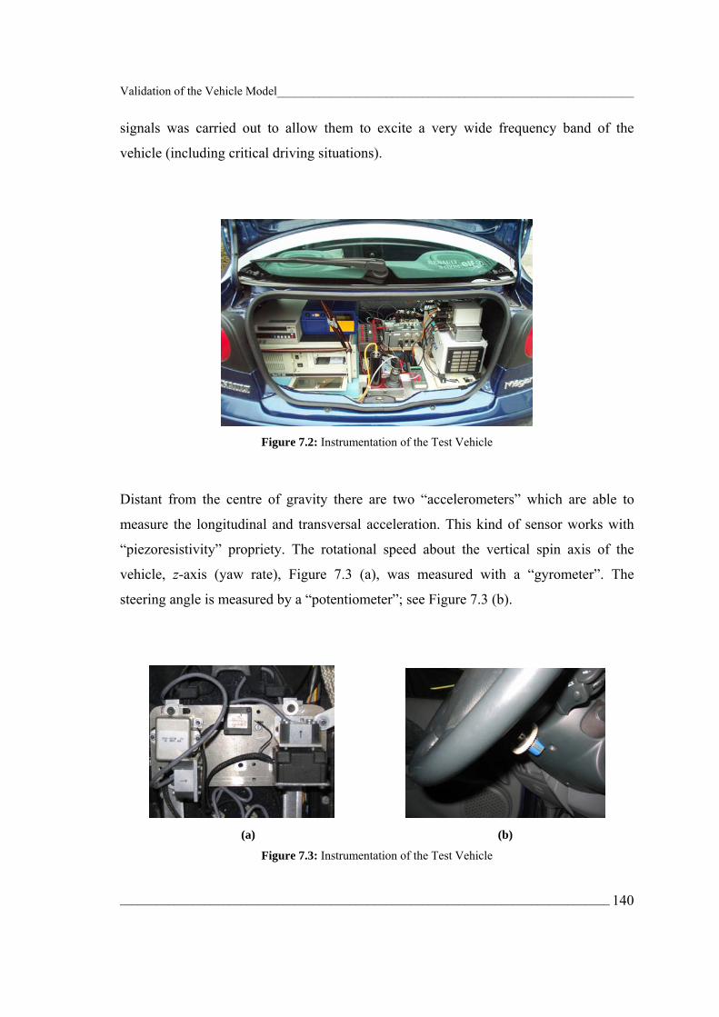
Validation of the Vehicle Model___________________________________________________________
_________________________________________________________________________________ 140
signals was carried out to allow them to excite a very wide frequency band of the
vehicle (including critical driving situations).
Figure 7.2: Instrumentation of the Test Vehicle
Distant from the centre of gravity there are two “accelerometers” which are able to
measure the longitudinal and transversal acceleration. This kind of sensor works with
“piezoresistivity” propriety. The rotational speed about the vertical spin axis of the
vehicle, z-axis (yaw rate), Figure 7.3 (a), was measured with a “gyrometer”. The
steering angle is measured by a “potentiometer”; see Figure 7.3 (b).
(a) (b) Figure 7.3: Instrumentation of the Test Vehicle

Validation of the Vehicle Model___________________________________________________________
_________________________________________________________________________________ 141
The longitudinal and transversal speeds are measured by an optical intermediate sensor
DATRON; see again Figure 7.2. This last instrument is very expensive, costing just
under ten thousand euros for one. An interesting alternative instrument for using this
model [42] is based on artificial intelligence techniques working through Fuzzy Logic.
7.2.6 Definition of Tests
In order to carry out validation, test drives were carried out with an experimental
vehicle, and the following variables recorded:
Model input variables Model output variables α Throttle opening u longitudinal velocity δ Steering angle ax acceleration in x-direction ay acceleration in y-direction r yaw rate
Table 7.1: Inputs and Outputs of the Validation Model
The validation model calculates, from the inputs α and δ, the outputs u, ax, ay, and r, so
that a direct comparison can be carried out between the model and experimental data.
Thus, in order to describe the functioning of the vehicle, two tests have been executed.
These tests include the principal driving characteristics which could show the mean
critical conditions.
In normal driving conditions, it is possible to take in account the easier tyre model
known, linear one. There are many tests which are able to investigate the behaviour of
the vehicle, [30, 31, 32, 33, 34, 35, 36]. For example, the braking test is able to study
the longitudinal behaviour.
Instead, the manoeuvres about angular dynamics can show the principal characteristic
of the transversal behaviour, the braking test in band will be able to study the lateral
behaviour in transient conditions. Last, the sinusoidal test can be able to study the
response for frequency of the vehicle model.
7.2.7 Circuit Test
According to Figure 7.3, two kind of experimental tests have been performed. Precisely,
these tests regard the bands 3 and 7. Referring to the track, clockwise sense, the second

Validation of the Vehicle Model___________________________________________________________
_________________________________________________________________________________ 142
curve had run with higher velocity in owing to its radius of curvature which was
smaller. Opposite means for the 7th band, that its excessive bend limits the fast
manoeuvreing. As well, the faster is characterized by an high deceleration.
7.2.8 Handling of Data
The acquisition data which comes from the experimental tests can not be utilized
directly. In fact, it is necessary to choose the frequency of measures sampling, in this
case it is 50 Hz. This frequency corresponds to the same one utilized by the acquisition
system which works on the test vehicle (Dspace/RT-LAB). In this way, the frequencies
of the system can be held.
Every acquisition system has tabulation in order to store the data. Once known these
latter we need to traduce this information in order to utilize it in our ambient work
(Matlab/Simulink). However, all the measurements are suffering from a lot of noises,
such as vibrations due to the motion of the vehicle, and noises due to mechanical origin
(rigid parts moving), and finally electrical noises which disturb the acquisition field.
For all these reasons a specific filter can be used. A good arrangement to improve the
ratio signal/noises can be obtained with a filtering of 10 Hz by a third order Low-Pass
filter.
Opposite, another kind of noise could be a malfunctioning of the instruments, of the
acquisition system, such as slip and setting.
Figure 7.4: Track used to Perform the Experimental Tests

Validation of the Vehicle Model___________________________________________________________
_________________________________________________________________________________ 143
Finally, all the measure chain can be exposed to many perturbations. Meanly, these
perturbations can be summarized in the following factors:
• No accuracy during the assembly and balancing of the sensors;
• DATRON sensor can be equipped in wrong way because its specifications do
not give exactly the working limit, such as the time response and many other
factors.
During the validation tests, some measurement problems have been presented, such as
problem af estimation for the velocity sensor (DATRON) and problem to initialize the
files while the acquisition system was beginning.
Some checks can be made to set completely all the sensor. For example, for the
accelerometer varying around ±90° and so verifying that the measure corresponds with
the acceleration of gravity. For the sensor to be able to measure the steering angle, it is
possible to make a completely round about its spin axis in order to verify if the measure
is equal to 2π rad.
The next step, before comparing the experimental data and the simulation results, is to
rearrange the values assumed by the variable. Two filter-values for the throttle opening
have been made. First, according to the values bigger than full opening and the second
about values smaller than zero.
Into the following sentences it will be reported the cycles (Matlab/Simulink) used to
clean the final vectors before the validation graphs, where the letter T means throttle
opening [%].
Filter 1 Filter 2 % Control about values bigger than 100% for x=1:length(T_tot), if T_tot(x)>100 disp('Filter 1') T_tot(x)=100; end end
% Control about values negative. for x=1:length(T_tot), if T_tot(x)<0 disp('Filter 2') T_tot(x)=0; end end
Table 2: Filters for the Handling Data

Validation of the Vehicle Model___________________________________________________________
_________________________________________________________________________________ 144
7.2.9 Analysis of the Results
In the following section, many graphs, Figure 7.5 to 7.24, will illustrate the comparison
of the experimental data and the simulation data. That means all the following diagrams
will show some differences between the data measured by the sensors and the results of
the mathematical model. The latter includes the front and rear wheel drive (FWD-
RWD). One may note that the FWD model presents lots resolution difficulty that the
rear one. Particularly, as illustrated FWD with non-linear tyre model is 8 D.O.F.
because the lateral forces depend by the load transfer, so to obtain the dynamic solution
it is required solving all the blocks model. The front traction has more interaction with
the longitudinal model than the rear model, which contains only the velocity
longitudinal as linkage.
Therefore, the simulated with FWD model in the 3th and 7th turn is illustrated, Figures
7.5, 7.6, 7.7, 7.8, 7.9, and 7.10.
First, the simulations carried out in the 3th curve are characterized by discordance in
terms of velocity. In fact, this comes from a transient problem. During the first part of
the throttle opening curve, it is possible to note a physical discordance between the
throttle opening and the longitudinal velocity. In fact, the velocity signal measured by
the sensor was different from that simulated; physically, this happens because the
vehicle had its velocity, due to the inertia forces. The theoretical model cannot
reproduce this phenomenon; therefore, in corresponding to a throttle opening null, there
is a velocity smaller than that measured. The incongruence could be annulled operating
a set up on the velocity of vehicle that means to begin to store data from a steady state
of the speed and so operate the tests manoeuvres.
The second difference could come from an oscillating measure of the longitudinal
acceleration which is, obviously, particularly stable in the model. In fact, in the model
the vibration noises are neglected.
Moreover, some differences, concerning the evaluation of inertia in the lateral model,
can be visualized. It is very clear for the non-linear tyre model because it is not able to
reproduce very well the real behaviour of the automobile. For this reason more
concordance could be obtained with the Pacejka model.

Validation of the Vehicle Model___________________________________________________________
_________________________________________________________________________________ 145
In 7th curve, according to the problem concerning the transient problem, shown in the
former sentence, the corresponding between the experimental data and simulation
results is sufficiently good. Only one problem is discovered, concerning the lateral
behaviour. In fact, while the steering angle presents a decreasing trend, in corresponding
of the time step 148, 232 and 403 seconds, the yaw rate and the lateral acceleration do
not have the same behaviour. Physically, this incongruence could come from imperfect
measurements. Taking care to the simulations 2, 3 and 5, there is not a good accordance
of the yawing rate for the fixed steering angle. In fact, there is a simple delay in terms of
the response. Probably, because the flexibility of the body is always present in realty.
Opposite in the model, hypnotizing the vehicle as a rigid body, the response in
transversal terms is instantaneous.
18 20 22 24 26-50
0
50
100Longitudinal Behavior
time [s]
Thro
ttle
[%]
measuredsimulated
18 20 22 24 26-100
-50
0
50
100Lateral Behavior
time [s]
Ste
erin
g A
ngle
[deg
]
measuredsimulated
18 20 22 24 2612
14
16
18
20
time [s]
Long
itudi
nal V
eloc
ity [m
/s]
measuredsimulated
18 20 22 24 26-0.5
0
0.5
1
time [s]
Yaw
ing
Rat
e [ra
d/s]
18 20 22 24 26-4
-2
0
2
4
time [s]Long
itudi
nal A
ccel
erat
ion
[m/s
2 ]
measuredsimulated
18 20 22 24 26-10
-5
0
5
10
time [s]
Late
ral A
ccel
erat
ion
[m/s
2 ]
measuredsimulated l tiresimulated l-d tiresimulated non-l-d tire
Figure 7.5: Experimental Test-Curve 3 Sim1, Simulated FWD.

Validation of the Vehicle Model___________________________________________________________
_________________________________________________________________________________ 146
186 188 190 192 194 196-50
0
50
100
150Longitudinal Behavior
time [s]
Thro
ttle
[%]
measuredsimulated
186 188 190 192 194 196-100
0
100
200Lateral Behavior
time [s]
Ste
erin
g A
ngle
[deg
]
measuredsimulated
186 188 190 192 194 19614
16
18
20
22
time [s]
Long
itudi
nal V
eloc
ity [m
/s]
measuredsimulated
186 188 190 192 194 196-0.5
0
0.5
1
time [s]
Yaw
ing
Rat
e [ra
d/s]
186 188 190 192 194 196-5
0
5
time [s]Long
itudi
nal A
ccel
erat
ion
[m/s
2 ]
measuredsimulated
186 188 190 192 194 196-10
0
10
20
time [s]
Late
ral A
ccel
erat
ion
[m/s
2 ]
measuredsimulated l tiresimulated l-d tiresimulated non-l-d tire
Figure 7.6: Experimental Test-Curve 3 Sim2, Simulated FWD.
58 60 62 64 66-20
0
20
40Longitudinal Behavior
time [s]
Thro
ttle
[%]
measuredsimulated
58 60 62 64 66-100
-50
0
50
100Lateral Behavior
time [s]
Ste
erin
g A
ngle
[deg
]
measuredsimulated
58 60 62 64 6620
22
24
26
time [s]
Long
itudi
nal V
eloc
ity [m
/s]
measuredsimulated
58 60 62 64 66-0.5
0
0.5
time [s]
Yaw
ing
Rat
e [ra
d/s]
58 60 62 64 66-4
-2
0
2
time [s]Long
itudi
nal A
ccel
erat
ion
[m/s
2 ]
measuredsimulated
58 60 62 64 66-10
-5
0
5
10
time [s]
Late
ral A
ccel
erat
ion
[m/s
2 ]
measuredsimulated l tiresimulated l-d tiresimulated non-l-d tire
Figure 7.7: Experimental Test-Curve 7 Sim1, Simulated FWD.

Validation of the Vehicle Model___________________________________________________________
_________________________________________________________________________________ 147
310 312 314 316 318-10
0
10
20
30Longitudinal Behavior
time [s]
Thro
ttle
[%]
measuredsimulated
310 312 314 316 318-50
0
50
100Lateral Behavior
time [s]
Ste
erin
g A
ngle
[deg
]
measuredsimulated
310 312 314 316 31820
22
24
26
28
time [s]
Long
itudi
nal V
eloc
ity [m
/s]
measuredsimulated
310 312 314 316 318-0.4
-0.2
0
0.2
0.4
time [s]
Yaw
ing
Rat
e [ra
d/s]
310 312 314 316 318-4
-2
0
2
time [s]Long
itudi
nal A
ccel
erat
ion
[m/s
2 ]
measuredsimulated
310 312 314 316 318-10
-5
0
5
10
time [s]
Late
ral A
ccel
erat
ion
[m/s
2 ]
measuredsimulated l tiresimulated l-d tiresimulated non-l-d tire
Figure 7.8: Experimental Test-Curve 7 Sim2, Simulated FWD.
480 482 484 486 488-20
0
20
40Longitudinal Behavior
time [s]
Thro
ttle
[%]
measuredsimulated
480 482 484 486 488-20
0
20
40
60Lateral Behavior
time [s]
Ste
erin
g A
ngle
[deg
]
measuredsimulated
480 482 484 486 48820
22
24
26
28
time [s]
Long
itudi
nal V
eloc
ity [m
/s]
measuredsimulated
480 482 484 486 488-0.4
-0.2
0
0.2
0.4
time [s]
Yaw
ing
Rat
e [ra
d/s]
480 482 484 486 488-3
-2
-1
0
1
time [s]Long
itudi
nal A
ccel
erat
ion
[m/s
2 ]
measuredsimulated
480 482 484 486 488-10
0
10
20
time [s]
Late
ral A
ccel
erat
ion
[m/s
2 ]
measuredsimulated l tiresimulated l-d tiresimulated non-l-d tire
Figure 7.9: Experimental Test-Curve 7 Sim3, Simulated FWD.

Validation of the Vehicle Model___________________________________________________________
_________________________________________________________________________________ 148
In the following section the simulation with RWD model is carried out. One has to note
that the longitudinal behaviour is always independent by the lateral one. Opposite is not
right. For this reason, even though the lateral model could not reproduce very well the
real data, the longitudinal model could have a good accordance.
18 20 22 24 26-50
0
50
100Longitudinal Behavior
time [s]
Thro
ttle
[%]
measuredsimulated
18 20 22 24 26-100
-50
0
50
100Lateral Behavior
time [s]
Ste
erin
g A
ngle
[deg
]
measuredsimulated
18 20 22 24 2612
14
16
18
20
time [s]
Long
itudi
nal V
eloc
ity [m
/s]
measuredsimulated
18 20 22 24 26-0.5
0
0.5
1
time [s]
Yaw
ing
Rat
e [ra
d/s]
18 20 22 24 26-4
-2
0
2
4
time [s]Long
itudi
nal A
ccel
erat
ion
[m/s
2 ]
measuredsimulated
18 20 22 24 26-10
-5
0
5
10
time [s]
Late
ral A
ccel
erat
ion
[m/s
2 ]
measuredsimulated l tiresimulated l-d tiresimulated non-l-d tire
Figure 7.10: Experimental Test-Curve 3 Sim1, Simulated RWD.

Validation of the Vehicle Model___________________________________________________________
_________________________________________________________________________________ 149
102 104 106 108 110 112-50
0
50
100
150Longitudinal Behavior
time [s]
Thro
ttle
[%]
measuredsimulated
102 104 106 108 110 112-100
0
100
200Lateral Behavior
time [s]
Ste
erin
g A
ngle
[deg
]
measuredsimulated
102 104 106 108 110 11210
15
20
25
time [s]
Long
itudi
nal V
eloc
ity [m
/s]
measuredsimulated
102 104 106 108 110 112-0.5
0
0.5
1
time [s]
Yaw
ing
Rat
e [ra
d/s]
102 104 106 108 110 112-4
-2
0
2
4
time [s]Long
itudi
nal A
ccel
erat
ion
[m/s
2 ]
measuredsimulated
102 104 106 108 110 112-10
-5
0
5
10
time [s]
Late
ral A
ccel
erat
ion
[m/s
2 ]
measuredsimulated l tiresimulated l-d tiresimulated non-l-d tire
Figure 7.11: Experimental Test-Curve 3 Sim2, Simulated RWD.
102 104 106 108 110 112-50
0
50
100
150Longitudinal Behavior
time [s]
Thro
ttle
[%]
measuredsimulated
102 104 106 108 110 112-100
0
100
200Lateral Behavior
time [s]
Ste
erin
g A
ngle
[deg
]
measuredsimulated
102 104 106 108 110 11210
15
20
25
time [s]
Long
itudi
nal V
eloc
ity [m
/s]
measuredsimulated
102 104 106 108 110 112-0.5
0
0.5
1
time [s]
Yaw
ing
Rat
e [ra
d/s]
102 104 106 108 110 112-4
-2
0
2
4
time [s]Long
itudi
nal A
ccel
erat
ion
[m/s
2 ]
measuredsimulated
102 104 106 108 110 112-10
-5
0
5
10
time [s]
Late
ral A
ccel
erat
ion
[m/s
2 ]
measuredsimulated l tiresimulated l-d tiresimulated non-l-d tire
Figure 7.12: Experimental Test-Curve 3 Sim2, Simulated RWD.
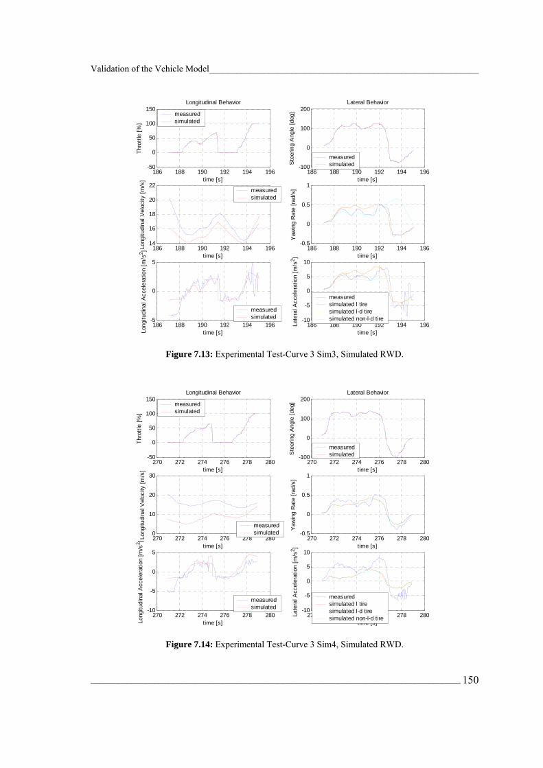
Validation of the Vehicle Model___________________________________________________________
_________________________________________________________________________________ 150
186 188 190 192 194 196-50
0
50
100
150Longitudinal Behavior
time [s]
Thro
ttle
[%]
measuredsimulated
186 188 190 192 194 196-100
0
100
200Lateral Behavior
time [s]
Ste
erin
g A
ngle
[deg
]
measuredsimulated
186 188 190 192 194 19614
16
18
20
22
time [s]
Long
itudi
nal V
eloc
ity [m
/s]
measuredsimulated
186 188 190 192 194 196-0.5
0
0.5
1
time [s]
Yaw
ing
Rat
e [ra
d/s]
186 188 190 192 194 196-5
0
5
time [s]Long
itudi
nal A
ccel
erat
ion
[m/s
2 ]
measuredsimulated
186 188 190 192 194 196-10
-5
0
5
10
time [s]
Late
ral A
ccel
erat
ion
[m/s
2 ]measuredsimulated l tiresimulated l-d tiresimulated non-l-d tire
Figure 7.13: Experimental Test-Curve 3 Sim3, Simulated RWD.
270 272 274 276 278 280-50
0
50
100
150Longitudinal Behavior
time [s]
Thro
ttle
[%]
measuredsimulated
270 272 274 276 278 280-100
0
100
200Lateral Behavior
time [s]
Ste
erin
g A
ngle
[deg
]
measuredsimulated
270 272 274 276 278 2800
10
20
30
time [s]
Long
itudi
nal V
eloc
ity [m
/s]
measuredsimulated
270 272 274 276 278 280-0.5
0
0.5
1
time [s]
Yaw
ing
Rat
e [ra
d/s]
270 272 274 276 278 280-10
-5
0
5
time [s]Long
itudi
nal A
ccel
erat
ion
[m/s
2 ]
measuredsimulated
270 272 274 276 278 280-10
-5
0
5
10
time [s]
Late
ral A
ccel
erat
ion
[m/s
2 ]
measuredsimulated l tiresimulated l-d tiresimulated non-l-d tire
Figure 7.14: Experimental Test-Curve 3 Sim4, Simulated RWD.

Validation of the Vehicle Model___________________________________________________________
_________________________________________________________________________________ 151
356 358 360 362 364 366-50
0
50
100Longitudinal Behavior
time [s]
Thro
ttle
[%]
measuredsimulated
356 358 360 362 364 366-50
0
50
100
150Lateral Behavior
time [s]
Ste
erin
g A
ngle
[deg
]
measuredsimulated
356 358 360 362 364 3665
10
15
20
25
time [s]
Long
itudi
nal V
eloc
ity [m
/s]
measuredsimulated
356 358 360 362 364 366-0.2
0
0.2
0.4
0.6
time [s]
Yaw
ing
Rat
e [ra
d/s]
356 358 360 362 364 366-5
0
5
time [s]Long
itudi
nal A
ccel
erat
ion
[m/s
2 ]
measuredsimulated
356 358 360 362 364 366-5
0
5
10
time [s]
Late
ral A
ccel
erat
ion
[m/s
2 ]
measuredsimulated l tiresimulated l-d tiresimulated non-l-d tire
Figure 7.15: Experimental Test-Curve 3 Sim5, Simulated RWD.
440 442 444 446 448 450-50
0
50
100Longitudinal Behavior
time [s]
Thro
ttle
[%]
measuredsimulated
440 442 444 446 448 450-100
0
100
200Lateral Behavior
time [s]
Ste
erin
g A
ngle
[deg
]
measuredsimulated
440 442 444 446 448 4505
10
15
20
25
time [s]
Long
itudi
nal V
eloc
ity [m
/s]
measuredsimulated
440 442 444 446 448 450-0.5
0
0.5
1
time [s]
Yaw
ing
Rat
e [ra
d/s]
440 442 444 446 448 450-5
0
5
time [s]Long
itudi
nal A
ccel
erat
ion
[m/s
2 ]
measuredsimulated 440 442 444 446 448 450
-10
-5
0
5
10
time [s]
Late
ral A
ccel
erat
ion
[m/s
2 ]
measuredsimulated l tiresimulated l-d tiresimulated non-l-d tire
Figure 7.16: Experimental Test-Curve 3 Sim6, Simulated RWD.

Validation of the Vehicle Model___________________________________________________________
_________________________________________________________________________________ 152
524 526 528 530 532 534-50
0
50
100Longitudinal Behavior
time [s]
Thro
ttle
[%]
measuredsimulated
524 526 528 530 532 534-100
0
100
200Lateral Behavior
time [s]
Ste
erin
g A
ngle
[deg
]
measuredsimulated
524 526 528 530 532 5345
10
15
20
25
time [s]
Long
itudi
nal V
eloc
ity [m
/s]
measuredsimulated
524 526 528 530 532 534-0.5
0
0.5
time [s]
Yaw
ing
Rat
e [ra
d/s]
524 526 528 530 532 534-5
0
5
time [s]Long
itudi
nal A
ccel
erat
ion
[m/s
2 ]
measuredsimulated
524 526 528 530 532 534-5
0
5
10
time [s]
Late
ral A
ccel
erat
ion
[m/s
2 ]
measuredsimulated l tiresimulated l-d tiresimulated non-l-d tire
Figure 7.17: Experimental Test-Curve 3 Sim7, Simulated RWD.
58 60 62 64 66-20
0
20
40Longitudinal Behavior
time [s]
Thro
ttle
[%]
measuredsimulated
58 60 62 64 66-100
-50
0
50
100Lateral Behavior
time [s]
Ste
erin
g A
ngle
[deg
]
measuredsimulated
58 60 62 64 6620
22
24
26
time [s]
Long
itudi
nal V
eloc
ity [m
/s]
measuredsimulated
58 60 62 64 66-0.5
0
0.5
time [s]
Yaw
ing
Rat
e [ra
d/s]
58 60 62 64 66-4
-2
0
2
time [s]Long
itudi
nal A
ccel
erat
ion
[m/s
2 ]
measuredsimulated
58 60 62 64 66-10
-5
0
5
10
time [s]
Late
ral A
ccel
erat
ion
[m/s
2 ]
measuredsimulated l tiresimulated l-d tiresimulated non-l-d tire
Figure 7.18: Experimental Test-Curve 7 Sim1, Simulated RWD.

Validation of the Vehicle Model___________________________________________________________
_________________________________________________________________________________ 153
142 144 146 148 150-20
0
20
40Longitudinal Behavior
time [s]
Thro
ttle
[%]
measuredsimulated
142 144 146 148 150-300
-200
-100
0
100Lateral Behavior
time [s]
Ste
erin
g A
ngle
[deg
]
measuredsimulated
142 144 146 148 15022
23
24
25
26
time [s]
Long
itudi
nal V
eloc
ity [m
/s]
measuredsimulated
142 144 146 148 150-2
-1
0
1
time [s]
Yaw
ing
Rat
e [ra
d/s]
142 144 146 148 150-4
-2
0
2
time [s]Long
itudi
nal A
ccel
erat
ion
[m/s
2 ]
measuredsimulated
142 144 146 148 150-60
-40
-20
0
20
time [s]
Late
ral A
ccel
erat
ion
[m/s
2 ]measuredsimulated l tiresimulated l-d tiresimulated non-l-d tire
Figure 7.19: Experimental Test-Curve 7 Sim2, Simulated RWD.
226 228 230 232 234-20
0
20
40
60Longitudinal Behavior
time [s]
Thro
ttle
[%]
measuredsimulated
226 228 230 232 234-600
-400
-200
0
200Lateral Behavior
time [s]
Ste
erin
g A
ngle
[deg
]
measuredsimulated
226 228 230 232 23420
22
24
26
time [s]
Long
itudi
nal V
eloc
ity [m
/s]
measuredsimulated
226 228 230 232 234-4
-2
0
2
time [s]
Yaw
ing
Rat
e [ra
d/s]
226 228 230 232 234-4
-2
0
2
time [s]Long
itudi
nal A
ccel
erat
ion
[m/s
2 ]
measuredsimulated
226 228 230 232 234-100
-50
0
50
time [s]
Late
ral A
ccel
erat
ion
[m/s
2 ]
measuredsimulated l tiresimulated l-d tiresimulated non-l-d tire
Figure 7.20: Experimental Test-Curve 7 Sim3, Simulated RWD.

Validation of the Vehicle Model___________________________________________________________
_________________________________________________________________________________ 154
310 312 314 316 318-10
0
10
20
30Longitudinal Behavior
time [s]
Thro
ttle
[%]
measuredsimulated
310 312 314 316 318-50
0
50
100Lateral Behavior
time [s]
Ste
erin
g A
ngle
[deg
]
measuredsimulated
310 312 314 316 31820
22
24
26
28
time [s]
Long
itudi
nal V
eloc
ity [m
/s]
measuredsimulated
310 312 314 316 318-0.2
0
0.2
0.4
0.6
time [s]
Yaw
ing
Rat
e [ra
d/s]
310 312 314 316 318-4
-2
0
2
time [s]Long
itudi
nal A
ccel
erat
ion
[m/s
2 ]
measuredsimulated
310 312 314 316 318-5
0
5
10
time [s]
Late
ral A
ccel
erat
ion
[m/s
2 ]
measuredsimulated l tiresimulated l-d tiresimulated non-l-d tire
Figure 7.21: Experimental Test-Curve 7 Sim4, Simulated RWD.
398 400 402 404 406-20
0
20
40
60Longitudinal Behavior
time [s]
Thro
ttle
[%]
measuredsimulated
398 400 402 404 406-600
-400
-200
0
200Lateral Behavior
time [s]
Ste
erin
g A
ngle
[deg
]
measuredsimulated
398 400 402 404 40615
20
25
30
time [s]
Long
itudi
nal V
eloc
ity [m
/s]
measuredsimulated
398 400 402 404 406-4
-2
0
2
time [s]
Yaw
ing
Rat
e [ra
d/s]
398 400 402 404 406-4
-2
0
2
time [s]Long
itudi
nal A
ccel
erat
ion
[m/s
2 ]
measuredsimulated
398 400 402 404 406-100
-50
0
50
time [s]
Late
ral A
ccel
erat
ion
[m/s
2 ]
measuredsimulated l tiresimulated l-d tiresimulated non-l-d tire
Figure 7.22: Experimental Test-Curve 7 Sim5, Simulated RWD.
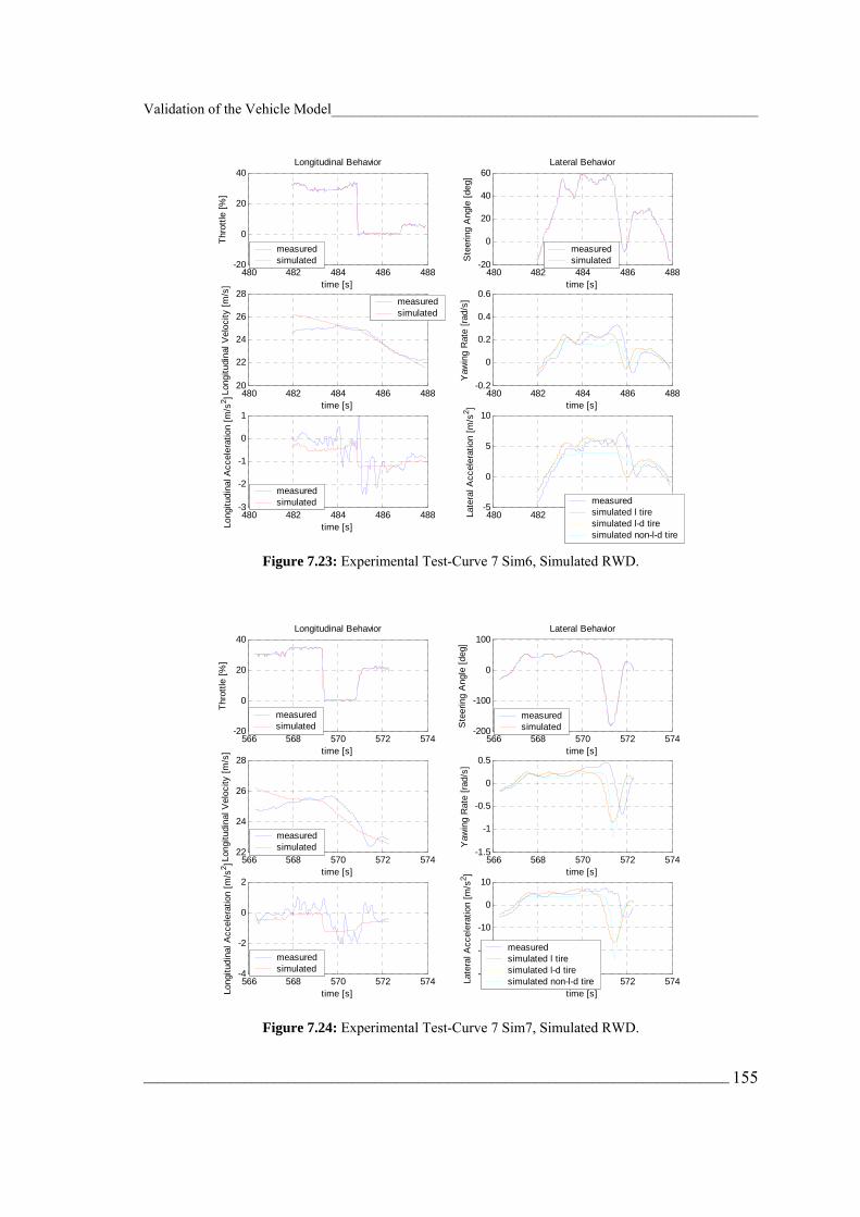
Validation of the Vehicle Model___________________________________________________________
_________________________________________________________________________________ 155
480 482 484 486 488-20
0
20
40Longitudinal Behavior
time [s]
Thro
ttle
[%]
measuredsimulated
480 482 484 486 488-20
0
20
40
60Lateral Behavior
time [s]
Ste
erin
g A
ngle
[deg
]
measuredsimulated
480 482 484 486 48820
22
24
26
28
time [s]
Long
itudi
nal V
eloc
ity [m
/s]
measuredsimulated
480 482 484 486 488-0.2
0
0.2
0.4
0.6
time [s]
Yaw
ing
Rat
e [ra
d/s]
480 482 484 486 488-3
-2
-1
0
1
time [s]Long
itudi
nal A
ccel
erat
ion
[m/s
2 ]
measuredsimulated
480 482 484 486 488-5
0
5
10
time [s]
Late
ral A
ccel
erat
ion
[m/s
2 ]
measuredsimulated l tiresimulated l-d tiresimulated non-l-d tire
Figure 7.23: Experimental Test-Curve 7 Sim6, Simulated RWD.
566 568 570 572 574-20
0
20
40Longitudinal Behavior
time [s]
Thro
ttle
[%]
measuredsimulated
566 568 570 572 574-200
-100
0
100Lateral Behavior
time [s]
Ste
erin
g A
ngle
[deg
]
measuredsimulated
566 568 570 572 57422
24
26
28
time [s]
Long
itudi
nal V
eloc
ity [m
/s]
measuredsimulated
566 568 570 572 574-1.5
-1
-0.5
0
0.5
time [s]
Yaw
ing
Rat
e [ra
d/s]
566 568 570 572 574-4
-2
0
2
time [s]Long
itudi
nal A
ccel
erat
ion
[m/s
2 ]
measuredsimulated
566 568 570 572 574-30
-20
-10
0
10
time [s]
Late
ral A
ccel
erat
ion
[m/s
2 ]
measuredsimulated l tiresimulated l-d tiresimulated non-l-d tire
Figure 7.24: Experimental Test-Curve 7 Sim7, Simulated RWD.

Validation of the Vehicle Model___________________________________________________________
_________________________________________________________________________________ 156
Concluding, one can say that the simulated longitudinal dynamics corresponds very
well to the measured data. Again the calculated values follow the measured data very
well. The longitudinal velocity is also well reproduced.
The noise about the longitudinal acceleration, which according to the measured data is
due to some extent dynamics, is simulated in the model as semi-constant value. This
could be different if oscillatory phenomena would have considered.
Similarly good results are given for the simulated lateral dynamics which shows only
small errors for the acceleration variable
In summary one can say that with sufficient excitation of the respective dynamics, the
longitudinal and lateral dynamics were very well reproduced.
The simulation model has proved itself suitable for calculation of the relevant drive
dynamics variables given steering angle and throttle opening.
_________________________________________________________________________________ 157
Chapter 8
8 Conclusions and Recommendations for Future Research
This work has proposed some foundation of mathematics, analytical methods, and
design strategies necessary to describe some characteristics of an automobile, so
exploitable for any application. Although the mathematics and simulations presented
herein can prove an useful intuitive understanding of generalized performance and
control characteristics of the vehicle. Understanding the nature of what has been done
here is essential in any future development of a vehicle simulation, even if a simple
modelling has been proposed . Having said this, we can now consider some of the
natural spin-offs of this research that must be considered in any future development
efforts.
8.1 Conclusion
One of the objectives of this work has been to develop a vehicle model that could be
used to predict the dynamics for steering and throttle regulation manoeuvres. The
dynamics for the complete vehicle have been presented but with many assumptions. In
fact, in this study only a non linear function for the lateral forces at the tyres has been
constructed. For all, the principal characteristics of the vehicle dynamics have been
performed.

Conclusions and Recommendations for Future Research_______________________________________
_________________________________________________________________________________ 158
8.1.1 Practical Use
One of the most important aspects of a computational study is its practical usefulness. In
other words, how the study can be used by other engineers and researchers. This study
can be helpful in many ways. First and foremost, it can be used as a basis for future
studies of optimization concepts applied to vehicle dynamics. This study may be
referenced to show that optimal paths can be generated by setting up the constrained
“optimization problem” using the unconstrained optimization algorithm of Matlab,
fmins.
Further, this research can be used as a preliminary study for the development of a new
“tyre testing procedure”. An accelerated tyre wear test path can be generated using the
tyre force maximization optimization routine. Often time, tyre manufacturers want to
compare the wear of different tyre constructions. By implementing this concept along
with a feedback steering controller, an automated testing procedure can be developed to
make tyre wear testing more efficient and accurate. Test vehicles are subjected to
automatically follow generated paths using the feedback steering controller, augmenting
the ability of the test drivers. Further, automatic testing improves repeatability by
consistently maintaining the same vehicle path while different sets of tyres are being
tested. As such, simulation such as those presented in this study can be used as a tool to
perform comparison tests on different vehicle specifications to determine the effects of
changing a certain parameter on the optimal path of the vehicle.
8.1.2 Improvement on Overall Approach
There are two issues that can be improved upon for this research, computation time and
model prediction accuracy. It is difficult to improve upon both issues at the same time
since they are strictly interrelated. Using a faster processor to perform the optimization
simulation, one can use higher degrees-of-freedom models or more accurate integration
routines, to increase the prediction accuracy.
A more efficient search algorithm can also be used to make the convergence rate of the
simulation faster. Genetics algorithm is a very attractive method to pursue. This method
is relative new to the field of engineering. There have been a few studies on using this

Conclusions and Recommendations for Future Research_______________________________________
_________________________________________________________________________________ 159
method in engineering applications [43]. The concept of genetics algorithm, however, is
relatively difficult to understand and even more difficult to implement in the simulation
algorithm.
Finally, a way to increase the speed of the simulation is to write the entyre simulation
program in Matlab script, C or C++ code. This entails efficiently writing loops, matrix
operations, algebraic operations, input/output of files, and other mathematical
manipulations in C or C++. Working into only an environment, such as the
Matlab/Simulink, the computational time could decrease rapidly. In fact, in our
software, mdl-file, we recall during each loop of integration S-function (which are
written in m-file). For this reason the process needs more time to converge.
Unfortunately, in this way we need also to implement a numeric method to solve the
differential equations.
8.2 Future Research
The research presented in this work has convinced us that the single track model is a
good option in the choice-design of the ground vehicles. In fact we have seen a part of
the dynamic performance, for all it was so quite complicated. We have also shown some
of the more significant issues, such as the adherence condition concept, non linear
linkage between the variables (such as it happens in the realty).
8.2.1 Optimal Control Methods
In the future an optimization method to vehicle dynamics could be applied to this study,
specifically to generate some optimal paths. In this case, the final goal could be to
minimize travel time, and to maximize tyre forces. Moreover, a parametric study, could
demonstrate the effectiveness of the optimization algorithm. These optimal paths could
be generated using optimization routine, such as the unconstrained optimization
algorithm of Matlab, fmins.

Conclusions and Recommendations for Future Research_______________________________________
_________________________________________________________________________________ 160
8.2.2 Parallel Processing Computation
To improve the computation speed of the optimization routine, a method such as the
parallel processing computation can be used to evaluate the optimization algorithm.
This method is consisted of using the UNIX platform workstation to run two processors
to evaluate the algorithm. This, however, would require some difficulties to implement
the algorithm. This method of computation will increase the speed of obtaining the
optimal solution. Furthermore, with an increase in computation speed, more
complicated vehicle and tyre models can be used.
8.2.3 Using Different Vehicle and Tyre Models
A further study can be performed to determine the effects of different vehicle and tyre
models. For the vehicle model, other degrees of freedom could be included, rolling
motion, pitching motion, and suspension effects. Obviously, other important dynamic
characteristics, such as the two masses motion have not taken into account. According
to before mathematical developments both could be presented and solved, also to
perform a three-dimensional vehicle and not plane-motion as we made.
As for the tyre model, a more current model can be used such as the Pacjeka tyre model.
This model requires using actual tyre data and fitting it with a form of least square
function.
At this time, according to the former, it may be considered another non linear behaviour
for the tyre model in the longitudinal direction. However, in this case, the solutions
required could be performed only by a numerical methods. Moreover, it should be
investigated in terms of ground slip in that direction.
Another focus of future work is experimental validation of the complete model while it
is moving on a discontinuous terrain, taking into account the vertical dynamics also.
This means taking into account a suspension model in order to have good information
about oscillatory phenomena. As known, these come from to common perturbations
always present at the wheels.
Lastly, include vehicle dynamic controllers such as traction control and yaw control into
the simulation to see the effects of these systems applied to determining an optimal

Conclusions and Recommendations for Future Research_______________________________________
_________________________________________________________________________________ 161
path. Another very interesting field of work surrounds to continuation of control
algorithms for the “ABS” concept [44]. In fact, we have suggested the single track
model but a double track model may provide distinct advantages in automatic field [45].
The dynamics for the braking manoeuvres have not been presented. However, it could
be interesting to include a brake model in order to investigate a braking-test in a turn.
Finally, work must be completed on the physical design of the real vehicle, with all its
topics. Many ideas concerning the typical problems of the vehicle have been considered
during this research. We hope that sometime in the future, this little model of the
ground-vehicle family will intrigue engineers and others to the same extent as it made
with the author. We believe it has already made a good start.

_________________________________________________________________________________ 162
Appendix A % % Vehicle_Dynamics_data m-file % Vehicle: Renault Mégane Coupé 16V 150 HP % input: Gas data, Vehicle data % output: Engine Map % % % GAS DATA % % % General data g = 9.806 ;% [m/s^2] Gravitational Acceleration % Gas data r0 = 8315.4 ;% [J kgmole/kg/K] Universal gas Constant mw = 28.97 ;% [kg/kgmole] Air Molecular Weight rair = r0/mw ; pcr = 0.528 ;% [/] Critical Pressure ratio rk = 1.4 ;% [/] Specific Heats ratio % Ambient data pair = 101300 ;% [Pa] Atmospheric Pressure tair = 300 ;% [K] Ambient Temperature umid = 50 ;% [%] Relative humidity rhoair=pair/rair/tair ;% [Kg/m3] Air Density % % VEHICLE DATA % % % Road data grade=[0, 0.02, 0.04, 0.06, 0.08, 0.10] ; % Transmission data % Renault DATA Megane etad=.8; taud = 3.8 ;% dif. gear ratio etacv=[0.80, 0.91, 0.93, 0.92, 0.95]; taucv=[3.7273,2.0476,1.3214,0.9667,0.7949] ;% JB1 type % taucv=[3.3636,1.8636,1.3214,0.9667,0.7949] % taucv=[3.0909,1.8636,1.3214,0.9667,0.7381] ;% JB3 type % taucv=[3.7273,2.0476,1.3214,0.9714,0.7561] ;% JB5 type % taucv=[3.3636,1.8636,1.3214,1.0294,0.8205] % Geometrical data rr =.300 ;% [m] Rolling Effective Radius J=1623.8 ;% [kgm^2] Inertia around z axle L=2.468 ;% [m] Wheelbase Vehicle L1=0.9552 ;% [m] semi-Wheelbase front Vehicle L2=L-L1 ;% [m] semi-Wheelbase rear Vehicle Lsensor=0.30 ;% [m] Distance from rear axle to the sensor position d=0.25 ;% [m] Relaxation length (or delay length) ratio_steer=20; % Tyre data C1=84085 ;% [Ns/rad] Cornering Stiffness of fornt tyre C2=87342 ;% [Ns/rad] Cornering Stiffness of rear tyre mu=.9 ;% [/] Coefficient of road adhesion h1=0.450 ;% [m] Legth between centre of gravity and ground h2=h1 ;% [m] Legth between point of application Faero and ground if(C1*L1<C2*L2) disp('Understeering Vehicle'); % Understeering/Oversteering Behaviour else disp('Oversteering Vehicle');

Appendix_____________________________________________________________________________
_________________________________________________________________________________ 163
end % Rigid driveline mc=2.8 ;% [kg] Crank Mass mcr=.3 ;% [kg] Connecting Rod Big End Mass rc=.03 ;% [m] Rc: Crank Radius ncyl=4 ;% [/] Cylinder Number ifw=.3 ;% [kgm^2] Flywheel Inertia icgi=((mc+mcr))*rc^2*ncyl ;% [kgm^2] Crank Gear Inertia iengine=icgi+ifw ;% [kgm^2] Total Engine Inertia Ieach_wheel=0.08 ;% [kgm^2] Wheel Inertia iwheel=Ieach_wheel*[(etad)/(taud)]^2 ;% [kgm^2] Equivalent Wheel Inertia mv_sprung=1202 ;% [kg] Sprung Mass of Vehicle mv_unsprung_front=105 ;% [kg] Unsprung front Mass of Vehicle mv_unsprung_rear=55 ;% [kg] Unsprung rear Mass of Vehicle mv=mv_sprung+mv_unsprung_front+mv_unsprung_rear ;% [kg] Total Mass of Vehicle ichassis=(mv*rr^2)*[(etad)/(taud)]^2 ;% [kgm^2] Equivalent Vehicle Inertia % Aereodynamics data cx = .328 ;% [/] Drag Coefficient Af=1.6 + 0.00056 * (mv-765) ;% [m^2] Frontal Area after J.Y.Wong "Theory of Groung Vehicle" sez=Af; % Engine data thvec=[0 20 30 40 50 60 70 80 85 100]; nevec=[0.8 1.2 1.6 2.0 2.4 2.8 3.2 3.6 5.0 5.4 5.8]*10^3; engine_map=[ 26.8204 -29.5025 -32.8550 -35.5371 -38.2191 -40.9012 -43.5832 -46.9358 -49.6178 -52.2999 -55.9819; 145.1599 78.4498 56.9934 45.2537 29.5025 19.4448 6.7051 -1.3410 -8.7166 -15.7512 -21.4564; 165.2752 139.4663 119.3509 99.2356 81.8023 69.7331 56.9934 45.2537 32.1845 22.1269 12.0692; 177.0149 175.3328 161.5931 146.8419 129.4086 111.9753 101.9177 89.1780 79.7908 65.3691 56.9934; 177.0149 187.0726 189.0841 185.3905 175.3328 159.5816 149.5239 139.4663 126.7266 115.6574 101.9177; 179.0264 195.4482 196.4597 199.1418 195.4482 185.3905 175.3328 171.6508 156.8996 142.1483 129.4086; 179.0264 199.1418 205.5058 205.5058 205.5058 201.8238 196.4597 189.0841 179.0264 166.9572 51.5355; 179.0264 201.8238 206.5174 209.1994 213.8930 216.5750 213.8930 211.8815 199.1418 187.0726 169.6393; 179.0264 201.8238 209.1994 213.8930 219.2571 219.2571 219.2571 219.2571 209.1994 196.4597 179.0264;
179.0264 201.8238 209.1994 213.8930 219.2571 223.9507 223.9507 223.9507 213.8930 205.5058185.3905 ];
figure(1) omega_engine=0:500:5000; plot(omega_engine,engine_map,'-') hold on title('Engine map') hold on xlabel('n_e [rpm]') ylabel('T_e [N m]') legend('th=0','th=20%','th=30%','th=40%','th=50%','th=60%','th=70%','th=80%','th=90%','th=100%',0) figure(2) omega_engine=0:500:5000; plot(omega_engine/5000,engine_map/223.9507,'-') hold on title('Adimensionless Engine map') hold on xlabel('n_e/n_emax [/]') ylabel('T_e/T_emax [/]') legend('th=0','th=20%','th=30%','th=40%','th=50%','th=60%','th=70%','th=80%','th=90%','th=100%',0) %close all tstep=0.02; tstop=120; disp('tstop 120')
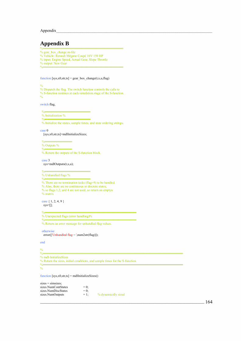
Appendix_____________________________________________________________________________
_________________________________________________________________________________ 164
Appendix B % % gear_box_change m-file % Vehicle: Renault Mégane Coupé 16V 150 HP % input: Engine Speed, Actual Gear, Slope Throttle % output: New Gear % function [sys,x0,str,ts] = gear_box_change(t,x,u,flag) % % Dispatch the flag. The switch function controls the calls to % S-function routines at each simulation stage of the S-function. % switch flag, % % Initialization % % % Initialize the states, sample times, and state ordering strings. case 0 [sys,x0,str,ts]=mdlInitializeSizes; % % Outputs % % % Return the outputs of the S-function block. case 3 sys=mdlOutputs(t,x,u); % % Unhandled flags % % % There are no termination tasks (flag=9) to be handled. % Also, there are no continuous or discrete states, % so flags 1,2, and 4 are not used, so return an emptyu % matrix case 1, 2, 4, 9 sys=[]; % % Unexpected flags (error handling)% % % Return an error message for unhandled flag values. otherwise error(['Unhandled flag = ',num2str(flag)]); end % % % mdl-InitializeSizes % Return the sizes, initial conditions, and sample times for the S-function. % % function [sys,x0,str,ts] = mdlInitializeSizes() sizes = simsizes; sizes.NumContStates = 0; sizes.NumDiscStates = 0; sizes.NumOutputs = 1; % dynamically sized

Appendix_____________________________________________________________________________
_________________________________________________________________________________ 165
sizes.NumInputs = 3; % dynamically sized sizes.DirFeedthrough = 1; % has direct feedthrough sizes.NumSampleTimes = 1; sys = simsizes(sizes); str = []; x0 = []; ts = [-1 0]; % inherited sample time % end mdl-InitializeSizes % % % mdl-Outputs % Return the output vector for the S-function % % function sys = mdlOutputs(t,x,u) if (u(3)>=0) if (u(1)>5000) % 5000 rpm Default Value switch (u(2)) case 1,2,3,4 disp(strcat('Change Velocity',num2str(u(2)+1))),sys(1)=u(2)+1; otherwise disp('Already in 5th Gear'),sys(1)=u(2); end elseif (u(1)==5000) % 5000 rpm Default Value disp('Velocity Engine equal to 5000') sys(1)=u(2); else disp('Velocity Engine lower than 5000') sys(1)=u(2); end else if (u(1)<2000) % 2000 rpm Default Value switch (u(2)) case 2,3,4,5 disp(strcat('Change Velocity',num2str(u(2)+1))),sys(1)=u(2)-1; otherwise disp('Already in 1th Gear'),sys(1)=u(2); end elseif (u(1)==2000) disp('Velocity Engine equal to 2000') sys(1)=u(2); else disp('Velocity Engine upper than 2000') sys(1)=u(2); end end end

Appendix_____________________________________________________________________________
_________________________________________________________________________________ 166
Appendix C % % Analytical Solution for Steering Pad test % Vehicle: Renault Mégane Coupé 16V 150 HP % input: Steering wheel angle % output: Lateral velocity, Yaw Rate % close all; tstep=0.002; tstop=1; J=1623.8 ;% [kgm^2] Inertia around z-axis (Izz) L=2.468 ;% [m] Wheelbase Vehicle L1=0.9552 ;% [m] semi-Wheelbase front Vehicle L2=L-L1 C1=84085 ;% Cornering Stiffness of front tyre C2=87342 ;% Cornering Stiffness of rear tyre % Transmission data % Renault Megane DATA etad=.8; etacv=[0.845, 0.904, 0.93, 0.948, 0.957]; taud = 3.87 ;% dif. gear ratio taucv=[3.7273, 2.0476, 1.3214, 0.9667, 0.7949] ;% JB1 type % Rigid driveline mc=2.5 ;% [kg] Crank Mass mcr=.35 ;% [kg] Connecting Rod Big End Mass rc=.04 ;% [m] Crank Radius ncyl=4 ;% [/] Cylinder Number ifw=.2 ;% [kgm^2] Flywheel Inertia icgi=((mc+mcr))*rc^2*ncyl ;% [kgm^2] Crank Gear Inertia iengine=icgi+ifw ;% [kgm^2] Total Engine Inertia Ieach_wheel=0.08 ;% [kgm^2] Wheel Inertia iwheel=Ieach_wheel*[(etad)/(taud)]^2 ;% [kgm^2] Equivalent Wheel Inertia mv_sprung=1202 ;% [kg] Sprung Mass of Vehicle mv_unsprung_front=105 ;% [kg] Un-sprung front Mass of Vehicle mv_unsprung_rear=55 ;% [kg] Un-sprung rear Mass of Vehicle mv=mv_sprung+mv_unsprung_front+mv_unsprung_rear ;% [kg] Total Mass of Vehicle u=20; delta=0.035 if(C1*L1<C2*L2) disp('Understeering Vehicle'); % Under-steering/Over-steering Behaviour else disp('Oversteering Vehicle'); end % A Matrix of coefficients a11=((C1+C2)/(mv*u)); a12=[((C1*L1)-(C2*L2))/(mv*u)]+u; a21=((C1*L1)-(C2*L2))/(J*u); a22=((C1*L1^2)+(C2*L2^2))/(J*u); A=-[a11 a12; a21 a22]; % Particular Solution Evaluation vp=[((C1*L2*L)-(mv*L1*u^2))*C1*u*delta]/[mv*J*u^2*det(A)]; rp=[C1*C2*L*u*delta]/[mv*J*u^2*det(A)]; beta_p=vp/u; Rp=(1/delta)*[L-[([(C1*L1)-(C2*L2)]/(C1*C2))*mv*u*u/L]]; alfa_1p=delta-[(vp+(rp*L1))/u]; alfa_2p=-(vp-(rp*L2))/u; if (alfa_1p>alfa_2p) disp('True only if the vehicle is understeering'); else disp('alfa_1p<alfa_2p because the vehicle is oversteering'); end
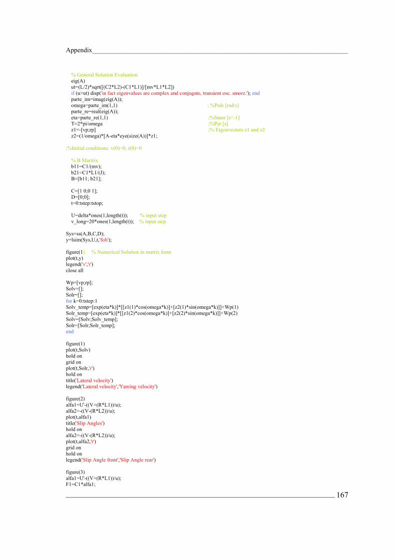
Appendix_____________________________________________________________________________
_________________________________________________________________________________ 167
% General Solution Evaluation eig(A) ut=(L/2)*sqrt([(C2*L2)-(C1*L1)]/[mv*L1*L2]) if (u>ut) disp('in fact eigenvalues are complex and conjugate, transient osc. smorz.'); end parte_im=imag(eig(A)); omega=parte_im(1,1) ; %Puls [rad/s] parte_re=real(eig(A)); eta=parte_re(1,1) ;%Smor [s^-1] T=2*pi/omega ;%Per [s] z1=-[vp;rp] ;% Eigenvectors z1 and z2 z2=(1/omega)*[A-eta*eye(size(A))]*z1; ;%Initial conditions: v(0)=0; r(0)=0 % B Martrix b11=C1/(mv); b21=C1*L1/(J); B=[b11; b21]; C=[1 0;0 1]; D=[0;0]; t=0:tstep:tstop; U=delta*ones(1,length(t)); % input step v_long=20*ones(1,length(t)); % input step Sys=ss(A,B,C,D); y=lsim(Sys,U,t,'foh'); figure(1) % Numerical Solution in matrix form plot(t,y) legend('v','r') close all Wp=[vp;rp]; Solv=[]; Solr=[]; for k=0:tstep:1 Solv_temp=[exp(eta*k)]*[[z1(1)*cos(omega*k)]+[z2(1)*sin(omega*k)]]+Wp(1) Solr_temp=[exp(eta*k)]*[[z1(2)*cos(omega*k)]+[z2(2)*sin(omega*k)]]+Wp(2) Solv=[Solv;Solv_temp]; Solr=[Solr;Solr_temp]; end figure(1) plot(t,Solv) hold on grid on plot(t,Solr,'r') hold on title('Lateral velocity') legend('Lateral velocity','Yawing velocity') figure(2) alfa1=U'-((V+(R*L1))/u); alfa2=-((V-(R*L2))/u); plot(t,alfa1) title('Slip Angles') hold on alfa2=-((V-(R*L2))/u); plot(t,alfa2,'r') grid on hold on legend('Slip Angle front','Slip Angle rear') figure(3) alfa1=U'-((V+(R*L1))/u); F1=C1*alfa1;

Appendix_____________________________________________________________________________
_________________________________________________________________________________ 168
plot(t,F1) title('Lateral forces') hold on alfa2=-((V-(R*L2))/u); F2=C2*alfa2; plot(t,F2,'r') grid on hold on legend('Lateral front force','Lateral rear force')

_________________________________________________________________________________ 169
References [1] N. W. Ressler, and D. J. Patterson, M. W. Soltis, , “Integrated Chassis and
Suspension Controls – Present and Future World of Chassis Electronic Controls”, IEEE International Congress on Transportation Electronics Proceedings, 1988.
[2] F. Gustafsson, “Estimation and Change Detection of Tyre – Road Friction
Using the Wheel Slip”, Proceedings of the 1996 IEEE International Symposium on Computer-Aided Control System Design, Dearborn, MI, September, 1996.
[3] J. Leih, “Semiactive Damping Control of Vibrations in Automobile”,
Transactions of the ASME Journal of Vibrations & Acoustics, Volume 115, July 1993.
[4] G. Yu, and I. K. Sethi, “Road-Following with Continuous Learning”,
Proceedings of the Intelligent Vehicles '95. Symposium, 1995. [5] M. Werner, and C. Engels, “A Nonlinear Approach to Vehicle Guidance”,
Proceedings of the Intelligent Vehicles '95. Symposium, 1995. [6] E. Freund, and R. Mayr, “Nonlinear Path Control in Automated Vehicle
Guidance”, IEEE Transactions on Robotics and Automation, Volume 13, No. 1, February 1997.
[7] A. Y. Maalej, D. A. Guenther, and J. R. Ellis, “Experimental Development of
Tyre Force and Moment Models”, International Journal of Vehicle Design, Volume 10, Number 1, 1989.
[8] L. Palkovics, “The Dynamics of Vehicles on Roads and on Tracks”, Supplement
to Vehicle Dynamics, Proceeding of the 15th IAVSD Symposium held in Budapest, (Hungary, August 25-29, 1997), Volume 29, 1998.
[9] http://www.adams.com/ [10] K. Yi and K. Hedrick, "Active and Semi-Active Heavy Truck Suspensions to
Reduce Pavement Damage," Society of Automotive Engineers (SAE) Paper, No. 892486, November 1989.
[11] H. Hatwal, and E. C. Mikulcik, "Some Inverse Solutions to an Automobile Path
Tracking Problem with Input Control of Steering and Brakes", Vehicle System Dynamics, Volume 15(1986), 1986.

References____________________________________________________________________________
_________________________________________________________________________________ 170
[12] J. P. M. Hendrikx, J. J. J. Meijlink, and R. F. C. Kriens, "Application of Optimal Control Theory to Inverse Simulation of Car Handling", Vehicle System Dynamics, Volume 26(1996), 1996.
[13] J. S. Arora, “Introduction to Optimum Design”, McGraw-Hill, Inc., New York,
1989. [14] D. E. Smith and J. M. Starkey, "Effects of Model Complexity on the
Performance of Automated Vehicle Steering Controllers: Model Development, Validation and Comparison", Vehicle System Dynamics, Volume 24(1995), 1995.
[15] J. P. Pauwelussen and H. B. Pacejka, "Smart Vehicles", Swets & Zeitlinger
Publishers, 1995. [16] G. Roppenecker, “Fahrzeugdynamik: Grundlagen der Modellierung und
Regelung”, AT Automatisierungstechnik 42, S. 429-441, 1995. [17] “Vehicle Dynamics Terminology”, SAE J670e, Society of Automotive
Engineers (SAE), Inc., Warrendale, PA, July 1976. [18] W. F. Milliken and D. L Milliken, “Race Car Vehicle Dynamics”, Society of
Automotive Engineers (SAE), Warrendale, PA, 1995. [19] T. D. Gillespie, “Fundamentals of Vehicle Dynamics”, Society of Automotive
Engineers (SAE), Inc., Warrendale, PA, 1992. [20] M. Guiggiani, “Dinamica del veicolo”, CittàStudi Edizioni, Torino, 1998. [21] M. Mitschke, “Dynamik der Kraftfahrzeuge”, Band A: Antrieb und Brehsung 3.
Auflage, Springer, Berlin, 1995. (Relax length) [22] J. Y. Wong, “Theory of Ground Vehicles”, John Wiley and Sons, Inc., New
York, 2001. [23] G. Genta, “Meccanica dell'autoveicolo”, Levrotto e Bella, 1997. [24] G. Genta, Motor Vehicle Dynamics, World Scientific Publishing , Singapore,
1997. [25] S. Bruni, “Appunti di Meccanica del Veicolo”, Dipartimento di Ingegneria
Meccanica, Politecnico di Milano, 2002. [26] J. Fredrikkson, and B. Egardt, “Integrated Powertrain: The Engine as an
Actuator”, Control and Automation Laboratory, Department of Signals and Systems, Chalmers University of Technology, SE-412 96 Göteborg, Sweden.

References____________________________________________________________________________
_________________________________________________________________________________ 171
[27] U. Kiencke and L. Nielsen, "Automotive Control Systems", Society of
Automotive Engineers (SAE), Inc., Warrendale, PA, 2000. [28] M. Mitschke, “Dynamik der Kraftfahrzeuge”, Band C: Fahrverhalten, Springer-
Verlag, Berlin, 1995. [29] A. R. Guido e L. Della Pietra, “Lezioni di meccanica delle macchine”, CUEN,
Napoli 1989. [30] ISO 3888, “Road Vehicles – Test procedure for a serve lane change
manoeuvre”, 1975. [31] ISO 4138, “Road vehicles – Steady state circular test procedure– Open-Loop
test procedure”, 1996. [32] ISO 7401, “Road vehicles – Lateral transient response test method”, 1988. [33] ISO 7975, “Road vehicles – Braking in a turn – Open-Loop test procedure”,
1985. [34] ISO 9816, “Road vehicles –Dropped throttle in a turn”, 1998. [35] ISO 8855, “Road vehicles – Vehicle dynamics and road holding ability –
Vocabulary”, 1991. [36] ISO 9816, “Passenger Cars – Power–off reactions of a vehicle in a turn – Open
loop test method”, 1993. [37] A. Porcel, “Contribution à la commande multivariable des systèmes complexes
rapides, instables ou pseudostables. Application au contrôle de stabilité de véhicules par approche «12 forces»,” Laboratoire de Modélisation Intelligence Processus et Systèmes (MIPS), Equipe de Modélisation et Identification en Automatique et Mécanique (MIAM), Ecole Supérieure des Science Appliquées pour l’Ingénieur (ESSAIM), Mulhouse, Décembre 2003.
[38] M. G. Vigier, “Pratique des Plans d’Expérience, Méthodologie Taguchi”. [39] G. Asch and al, “Acquisition de Données du Capteur à l’Ordinateur”. [40] Brűel and Kjaer, “Accéléromètres Piézoélectrique”, Théorie d’Applications,
1979. [41] J. Radix, , “Misures de Navigation”, Publication Techniques d’Ingénieur, 1990.

References____________________________________________________________________________
_________________________________________________________________________________ 172
[42] A. Porcel, C. Runde, M. Basset, and G. L. Gissinger, “Neuro-Fuzzy Approach to Real Time Total Velocity Estimation of a Passenger Car Covering Critical Situations ”, IFAC Workshop, Ohio, USA, Proc. 29-36, 1998.
[43] Gen, M., Genetic Algorithms and Engineering Design, Wiley & Sons, New
York, 1997. [44] G. L. Gissinger et N. Le Fòrt-Piat, “Systèmes automatisés: Contrôle-commande
de la voiture”, Lavoisier, Paris, 2002. [45] G. L. Gissinger et N. Le Fòrt-Piat, “Systèmes automatisés: La voiture
intelligente”, Lavoisier, Paris, 2002.