Embed Size (px)
Citation preview

MODELLING AND SIMULATION OF
SINGLE DIELECTRIC BARRIER DISCHARGE
PLASMA ACTUATORS
A Dissertation
Submitted to the Graduate School
of the University of Notre Dame
in Partial Fulfillment of the Requirements
for the Degree of
Doctor of Philosophy
by
Dmitriy M. Orlov, B.S., M.S.A.E.
Thomas C. Corke, Director
Graduate Program in Aerospace and Mechanical Engineering
Notre Dame, Indiana
October 2006

c© Copyright by
Dmitriy M. Orlov
2006
All Rights Reserved

MODELLING AND SIMULATION OF
SINGLE DIELECTRIC BARRIER DISCHARGE
PLASMA ACTUATORS
Abstract
by
Dmitriy M. Orlov
This work presents the study of the single-dielectric barrier discharge aerody-
namic plasma actuator. The physics of the plasma discharge was studied through
the time-resolved light intensity measurements of the plasma illumination. Plasma
characteristics were obtained and analyzed for a range of applied voltage ampli-
tudes and a.c. frequencies.
Based on this data, electro-static and lumped-element circuit models were
developed. The time-dependent charge distribution was used to provide boundary
conditions to the electric field equation that was used to calculate the actuator
body force vector. Numerical flow simulations were performed to study the effect
of the plasma body force on the neutral fluid. The results agreed well with the
experiments.
An application of the plasma actuators to the leading-edge separation control
on the NACA 0021 airfoil was studied numerically. The results were obtained
for a range of angles of attack for uncontrolled flow, steady and unsteady plasma
actuation. The aerodynamic stall of the airfoil was studied. Improvement in
the airfoil characteristics was observed in numerical simulations at high angles of

Dmitriy M. Orlov
attack in cases with plasma actuation. The computational results corresponded
very well with experimental observations.

In memory of Mikhail Aleksandrovich Vostrikov.
ii

CONTENTS
FIGURES . . . . . . . . . . . . . . . . . . . . . . . . . . . . . . . . . . . . v
ACKNOWLEDGMENTS . . . . . . . . . . . . . . . . . . . . . . . . . . . xii
CHAPTER 1: INTRODUCTION . . . . . . . . . . . . . . . . . . . . . . . 11.1 Background . . . . . . . . . . . . . . . . . . . . . . . . . . . . . . 11.2 Objectives . . . . . . . . . . . . . . . . . . . . . . . . . . . . . . . 13
CHAPTER 2: PHYSICAL PROPERTIES OF PLASMA ACTUATOR. . . 15
CHAPTER 3: ELECTRO-STATIC MODEL . . . . . . . . . . . . . . . . . 373.1 Mathematical and Numerical Formulation . . . . . . . . . . . . . 37
3.1.1 Electro-static Model . . . . . . . . . . . . . . . . . . . . . 383.1.1.1 Governing equations for electro-static problem and body
force . . . . . . . . . . . . . . . . . . . . . . . . . . . . . 383.1.1.2 Numerical Formulation of Electro-static Problem . . . . 443.1.2 Flow Problem . . . . . . . . . . . . . . . . . . . . . . . . . 473.1.2.1 Governing Equations for Flow Problem . . . . . . . . . . 473.1.2.2 Boundary Conditions . . . . . . . . . . . . . . . . . . . . 483.1.2.3 Model Problem . . . . . . . . . . . . . . . . . . . . . . . 513.1.2.4 Numerical Formulation of Flow Problem . . . . . . . . . 52
3.2 Results . . . . . . . . . . . . . . . . . . . . . . . . . . . . . . . . . 543.2.1 Body Force Results . . . . . . . . . . . . . . . . . . . . . . 543.2.2 Flow Problem Results with Spatially Weighted Body Force 693.2.3 Flow Problem Results with Temporally-spatially weighted
body force. . . . . . . . . . . . . . . . . . . . . . . . . . . 80
CHAPTER 4: LUMPED-ELEMENT CIRCUIT MODEL . . . . . . . . . . 914.1 Spatial Lumped-Element Circuit Model . . . . . . . . . . . . . . . 91
4.1.1 Mathematical Formulation . . . . . . . . . . . . . . . . . . 91
iii

4.1.2 Numerical Formulation of Temporal Lumped-Element Cir-cuit Model . . . . . . . . . . . . . . . . . . . . . . . . . . . 97
4.1.3 Results . . . . . . . . . . . . . . . . . . . . . . . . . . . . . 984.2 Spatial-Temporal Lumped-Element Circuit Model . . . . . . . . . 107
4.2.1 Mathematical Formulation . . . . . . . . . . . . . . . . . . 1074.2.2 Numerical Formulation of Space-Time Lumped-Element Cir-
cuit Model . . . . . . . . . . . . . . . . . . . . . . . . . . . 1144.2.3 Results of Space-Time Lumped-Element Circuit Model . . 116
CHAPTER 5: MODELING OF LEADING-EDGE SEPARATION CON-TROL USING PLASMA ACTUATORS. . . . . . . . . . . . . . . . . . 1415.1 Background . . . . . . . . . . . . . . . . . . . . . . . . . . . . . . 1415.2 Problem Formulation . . . . . . . . . . . . . . . . . . . . . . . . . 1425.3 Results . . . . . . . . . . . . . . . . . . . . . . . . . . . . . . . . . 153
CHAPTER 6: CONCLUSIONS AND RECOMMENDATIONS FOR FU-TURE WORK . . . . . . . . . . . . . . . . . . . . . . . . . . . . . . . 1736.1 Conclusions . . . . . . . . . . . . . . . . . . . . . . . . . . . . . . 173
6.1.1 Physics of Discharge . . . . . . . . . . . . . . . . . . . . . 1736.1.2 Electrostatic Model . . . . . . . . . . . . . . . . . . . . . . 1756.1.3 Lumped-element Circuit Model . . . . . . . . . . . . . . . 1766.1.4 Leading-edge Separation Control . . . . . . . . . . . . . . 178
6.2 Recommendations For Future Work . . . . . . . . . . . . . . . . . 1806.2.1 Physical Properties of Plasma Discharge . . . . . . . . . . 1806.2.2 Improvements to the Lumped-element Circuit Model . . . 1816.2.3 Applications . . . . . . . . . . . . . . . . . . . . . . . . . . 183
BIBLIOGRAPHY . . . . . . . . . . . . . . . . . . . . . . . . . . . . . . . 184
iv

FIGURES
1.1 The aerodynamic plasma actuator in a chord-wise section. . . . . 2
1.2 The dielectric barrier discharge is self-limiting because charge buildupon the dielectric surface opposes the voltage applied across theplasma, when the applied voltage is negative going (a), or the chargetransferred through the plasma is limited to that deposited on thedielectric surface, when the voltage reverses (b). . . . . . . . . . . 4
2.1 Experimental setup used in measuring plasma light emission forSDBD model validation. . . . . . . . . . . . . . . . . . . . . . . . 16
2.2 Schematic of experimental setup used in measuring plasma lightemission. . . . . . . . . . . . . . . . . . . . . . . . . . . . . . . . . 17
2.3 Representative voltage (a), current (b) and PMT output (c) timeseries for SDBD plasma actuator. . . . . . . . . . . . . . . . . . . 18
2.4 Space-time variation of the measured plasma light emission forSDBD plasma actuator corresponding to one period, T , of the inputa.c. cycle. . . . . . . . . . . . . . . . . . . . . . . . . . . . . . . . 20
2.5 Contour lines of space-time variation of the measured plasma lightemission for SDBD plasma actuator corresponding to one period,T , of the input a.c. cycle. . . . . . . . . . . . . . . . . . . . . . . 21
2.6 Plasma sweep velocity as function of applied voltage amplitude. . 22
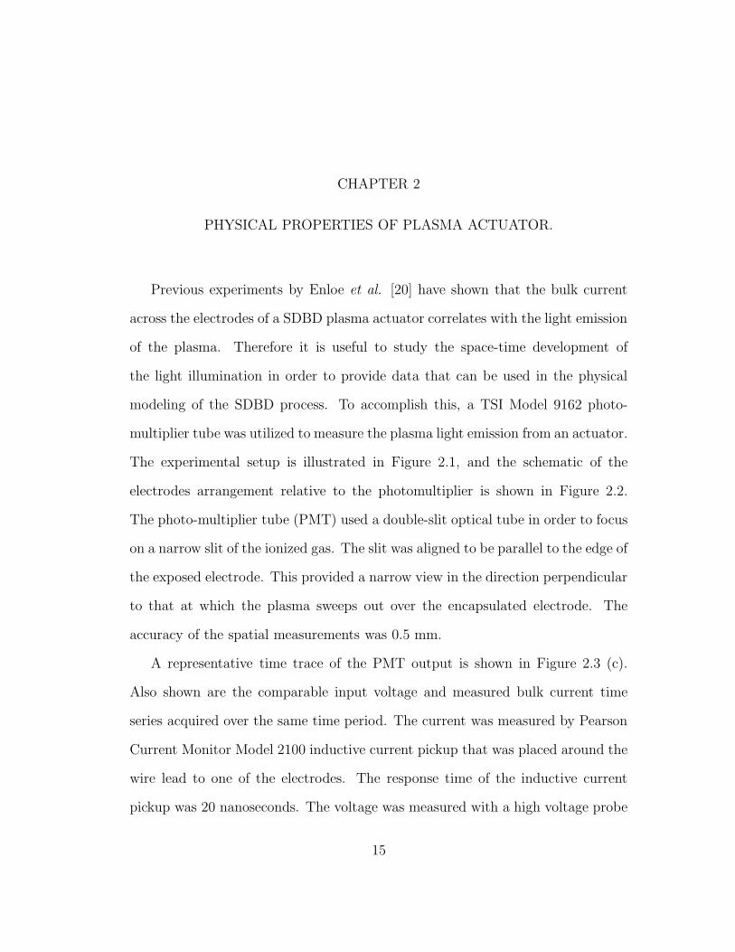
2.7 Maximum plasma extent as function of applied voltage amplitude. 23
2.8 Space-time variation of the measured plasma light emission forSDBD plasma actuator at Vapp = 5 kV and fa.c. = 5 kHz. . . . . . 25
2.9 Space-time variation of the measured plasma light emission forSDBD plasma actuator at Vapp = 5 kV and fa.c. = 6 kHz. . . . . . 26
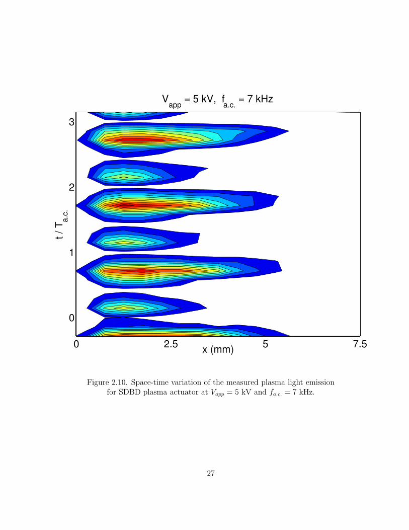
2.10 Space-time variation of the measured plasma light emission forSDBD plasma actuator at Vapp = 5 kV and fa.c. = 7 kHz. . . . . . 27
2.11 Space-time variation of the measured plasma light emission forSDBD plasma actuator at Vapp = 5 kV and fa.c. = 8 kHz. . . . . . 28
v

2.12 Space-time variation of the measured plasma light emission forSDBD plasma actuator at Vapp = 5 kV and fa.c. = 9 kHz. . . . . . 29
2.13 Space-time variation of the measured plasma light emission forSDBD plasma actuator at Vapp = 5 kV and fa.c. = 10 kHz. . . . . 30
2.14 Space-time variation of the measured plasma light emission forSDBD plasma actuator at Vapp = 5 kV and fa.c. = 11 kHz. . . . . 31
2.15 Plasma sweep velocity as function of applied a.c. frequency. . . . 32
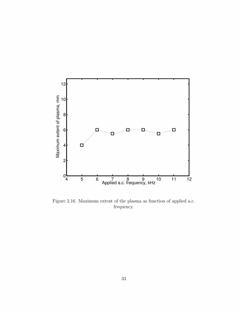
2.16 Maximum extent of the plasma as function of applied a.c. frequency. 33
2.17 Total light emission for SDBD plasma actuator as function of ap-plied a.c. frequency. . . . . . . . . . . . . . . . . . . . . . . . . . . 34
2.18 Total light intensity from the plasma actuator as function of appliedvoltage amplitude. . . . . . . . . . . . . . . . . . . . . . . . . . . 35
3.1 One-dimensional electric field acting on the charges. . . . . . . . . 40
3.2 Rectangular computational domain with solid boundaries. . . . . 49
3.3 Computational domain with two electrodes separated by the dielec-tric. . . . . . . . . . . . . . . . . . . . . . . . . . . . . . . . . . . 55
3.4 Numerical grid for the electro-static problem with Robert’s stretch-ing applied to resolve electric field and body force near the electrodes. 59
3.5 Zoomed-in view of the numerical grid for the electro-static problemwith Robert’s stretching applied to resolve electric field and bodyforce near the electrodes. . . . . . . . . . . . . . . . . . . . . . . . 60
3.6 Electric potential ϕ as a function of space coordinates. . . . . . . 61
3.7 Lines of constant electric potential near inner edge of electrodes. . 62
3.8 Electric field ~E in the upper part of the domain (air), near innerelectrodes’ edges. . . . . . . . . . . . . . . . . . . . . . . . . . . . 63
3.9 Body force as result of electro-static equation solution. . . . . . . 64
3.10 Body force on the fluid flow scale. . . . . . . . . . . . . . . . . . . 65
3.11 Incorrect flow resulting from non-weighted body force. The largestvelocity vector corresponds to |V | = 2 m/s. . . . . . . . . . . . . . 66
3.12 Spatial variation of light intensity from the plasma actuator. . . . 68
3.13 Spatially-weighted body force. . . . . . . . . . . . . . . . . . . . . 70
3.14 Computational domain, normalized by Xmax and Ymax, actuatorlocated on the bottom surface at X = 0.5. . . . . . . . . . . . . . 71
3.15 Body force is introduced into the Navier-Stokes equations at timet = 0. . . . . . . . . . . . . . . . . . . . . . . . . . . . . . . . . . . 73
vi

3.16 “Starting” vortex near actuators at t = 0.25ms. The largest veloc-ity vector corresponds to |V | = 1.5 m/s. . . . . . . . . . . . . . . 74
3.17 “Starting” vortex near actuators at t = 1.25ms. The largest veloc-ity vector corresponds to |V | = 3 m/s. . . . . . . . . . . . . . . . 75
3.18 PIV setup by Post [61]. . . . . . . . . . . . . . . . . . . . . . . . . 76
3.19 PIV laser trigger setup by Post [61]. . . . . . . . . . . . . . . . . . 76
3.20 “Starting” vortex at t = 2, 12, 35, 60 ms, PIV results by Post [61]. 77
3.21 Velocity field of the developed jet flow at T → ∞.The largest ve-locity vector corresponds to |V | = 4.7 m/s. . . . . . . . . . . . . . 78
3.22 Developed jet flow at T → ∞, PIV results by Post [61]. . . . . . . 79
3.23 Magnitude of the space-time weighting function used on the electro-static body force for one half of the a.c. cycle. . . . . . . . . . . . 81
3.24 Method for introducing space-time weighting of electro-static bodyforce during time-steps of the Navier-Stokes solver. . . . . . . . . 82
3.25 x-component velocity profiles normalized by maximum velocitiesand the locations of maximum velocities at different locations down-stream of the simulated actuator with spatial weighting of the bodyforce and the steady (long-time) solution. . . . . . . . . . . . . . . 84
3.26 x-component velocity profiles taken at X = 0.5938 for differenttimes following the impulsive start of the actuator body force. Bodyforce is spatially weighted only. . . . . . . . . . . . . . . . . . . . 85
3.27 x-component velocity profiles taken at X = 0.5938 for differenttimes following the impulsive start of the actuator body force. Bodyforce is spatially-temporally weighted. . . . . . . . . . . . . . . . . 86
3.28 Maximum x-component velocity as a function of time for impul-sively started actuator body force. Star indicates first-order timeconstant corresponding to where U
Ut→∞
= 1e. . . . . . . . . . . . . . 87
3.29 Maximum induced velocity in electro-static actuator model as afunction of voltage. . . . . . . . . . . . . . . . . . . . . . . . . . . 89
4.1 Spatial lumped-element circuit model of a single dielectric barrierdischarge plasma actuator. . . . . . . . . . . . . . . . . . . . . . . 93
4.2 Schenatic showing three node points where voltage is followed inthe circuit in the spatial lumped-element circuit model of a singledielectric barrier discharge plasma actuator. . . . . . . . . . . . . 95
vii

4.3 Voltage time series for α = 0.1 and α = 0.2: applied voltage (solidline), surface voltage (dashed line), voltage difference (dotted line),and plasma threshold (dash-dotted line). . . . . . . . . . . . . . . 100
4.4 Voltage time series for α = 0.3 and α = 0.4: applied voltage (solidline), surface voltage (dashed line), voltage difference (dotted line),and plasma threshold (dash-dotted line). . . . . . . . . . . . . . . 101
4.5 Applied voltage and rectified current in the circuit, experimentalresults. . . . . . . . . . . . . . . . . . . . . . . . . . . . . . . . . . 102
4.6 Average dissipated power as a function of the applied voltage basedon the actuator model. . . . . . . . . . . . . . . . . . . . . . . . . 104
4.7 Dependence of plasma actuator maximum induced velocity (opensymbols) and plasma dissipated power based on lumped-elementcircuit model(closed symbols as a function of applied a.c. voltage. 105
4.8 Maximum extent of the plasma as function of applied voltage am-plitude for temporal lumped-element circuit model simulation andexperiments (Enloe [20] and present). . . . . . . . . . . . . . . . . 106
4.9 The physical space over the encapsulated electrode is divided intoN sub-regions. . . . . . . . . . . . . . . . . . . . . . . . . . . . . . 108
4.10 Electric circuit model of a single dielectric aerodynamic plasmaactuator. . . . . . . . . . . . . . . . . . . . . . . . . . . . . . . . . 109
4.11 Schematic drawing of the n-th air capacitor. . . . . . . . . . . . . 110
4.12 Schematic drawing of the n-th dielectric capacitor. . . . . . . . . . 111
4.13 Maximum value of the plasma body force as function of the numberof parallel networks. . . . . . . . . . . . . . . . . . . . . . . . . . 113
4.14 Voltage on the surface of the dielectric in the first five sub-circuits(n=1,2,3,4,5) obtained from space-time lumped element circuit model.117
4.15 Plasma current in the first five sub-circuits (n=1,2,3,4,5) obtainedfrom space-time lumped element circuit model. . . . . . . . . . . . 118
4.16 Rectified plasma current for one a.c. period of input obtained fromspace-time lumped element circuit model. . . . . . . . . . . . . . . 120
4.17 Contour lines of constant rectified plasma current obtained fromspace-time lumped element circuit model. . . . . . . . . . . . . . . 121
4.18 Comparison between space-time model and experiments for themaximum plasma extent over covered electrode as function of voltage.123
4.19 Comparison between space-time model and experiment for plasmasweep velocity as function of voltage. . . . . . . . . . . . . . . . . 124
viii

4.20 Comparison between space-time model and experiment for maxi-mum extent of the plasma as function of applied a.c. frequency. . 125
4.21 Comparison between space-time model and experiment for plasmasweep velocity as function of applied a.c. frequency. . . . . . . . . 126
4.22 Computational domain for calculation of unsteady plasma body force.128
4.23 Normalized plasma bodyforce magnitude as function of time andposition over covered electrode. . . . . . . . . . . . . . . . . . . . 130
4.24 Normalized maximum value of the plasma bodyforce magnitude asfunction of time. Dots indicate where the snapshots of the bodyforce vector fields are taken. . . . . . . . . . . . . . . . . . . . . . 131
4.25 Plasma body force vector field and body force amplitude at t =0.2 · Ta.c.. The body force is normalized by the maximum value inthe a.c. cycle. . . . . . . . . . . . . . . . . . . . . . . . . . . . . . 132
4.26 Plasma body force vector field at t = 0.4 · Ta.c.. The body force isnormalized by the maximum value in the a.c. cycle. . . . . . . . . 133
4.27 Plasma body force vector field at t = 0.7 · Ta.c.. The body force isnormalized by the maximum value in the a.c. cycle. . . . . . . . . 134
4.28 Plasma body force vector field at t = 0.9 · Ta.c.. The body force isnormalized by the maximum value in the a.c. cycle. . . . . . . . . 135
4.29 Spectrum of the plasma body force obtained with space-time lumped-element circuit model. . . . . . . . . . . . . . . . . . . . . . . . . 137
4.30 Effect of dielectric material on plasma body force. . . . . . . . . . 138
4.31 Effect of dielectric material on power dissipated by the plasma ac-tuator. . . . . . . . . . . . . . . . . . . . . . . . . . . . . . . . . . 139
5.1 Schematic of the plasma actuator on the leading edge of NACA0021 airfoil for body force computations. . . . . . . . . . . . . . . 144
5.2 Unstructured grid near leading edge of NACA 0021 airfoil for plasmabody force computations. . . . . . . . . . . . . . . . . . . . . . . . 145
5.3 Computed steady plasma body force vectors near leading edge ofNACA 0021 airfoil, shown on structured computational grid usedfor flow solver. . . . . . . . . . . . . . . . . . . . . . . . . . . . . . 146
5.4 Full view of computational grid used for the flow simulation of theNACA 0021 airfoil. . . . . . . . . . . . . . . . . . . . . . . . . . . 147
5.5 Zoomed-in view of computational grid showing grid point clusteringin the region of the boundary layer. . . . . . . . . . . . . . . . . . 148
ix

5.6 Lift and drag coefficients convergence history at 5 degrees angle ofattack, Ufs = 35 m/s, uncontrolled flow. . . . . . . . . . . . . . . 155
5.7 Lift and drag coefficients convergence history at 25 degrees angleof attack, Ufs = 35 m/s, uncontrolled flow. . . . . . . . . . . . . . 156
5.8 Lift coefficient versus angle of attack at Ufs = 35 m/s for uncon-trolled flow. . . . . . . . . . . . . . . . . . . . . . . . . . . . . . . 157
5.9 Example of short duty cycle a.c. input for unsteady operation ofplasma actuators (a) and its numerical representation (b). . . . . 159
5.10 Velocity vector field near leading edge of airfoil at t = 0.00001 sec-onds after the impulsive start of the actuator. The largest velocityvector corresponds to |V | = 4.03 m/s. . . . . . . . . . . . . . . . . 160
5.11 Velocity vector field near leading edge of airfoil at t = 0.02 secondsafter the impulsive start of the actuator. The largest velocity vectorcorresponds to |V | = 8.34 m/s. . . . . . . . . . . . . . . . . . . . . 161
5.12 Velocity vector field near leading edge of airfoil at t = 0.06 secondsafter the impulsive start of the actuator. The largest velocity vectorcorresponds to |V | = 8.36 m/s. . . . . . . . . . . . . . . . . . . . . 162
5.13 Velocity vector field near leading edge of airfoil at t = 0.18 secondsafter the impulsive start of the actuator. The largest velocity vectorcorresponds to |V | = 8.37 m/s. . . . . . . . . . . . . . . . . . . . . 163
5.14 Velocity vector field (a) and contour lines of λ2 = 0 (b) at t =0.01743 seconds in still air. The plasma actuator is working inunsteady mode at 120 Hz. The largest velocity vector correspondsto |V | = 4.49 m/s. . . . . . . . . . . . . . . . . . . . . . . . . . . 164
5.15 Contour lines of stream function (a) and λ2 = 0 (b), no actuation,23 degrees angle of attack. . . . . . . . . . . . . . . . . . . . . . . 165
5.16 Contour lines of stream function (a) and λ2 = 0 (b) for steadyactuation, 23 degrees angle of attack. . . . . . . . . . . . . . . . . 166
5.17 Contour lines of stream function (a) and λ2 = 0 (b) for unsteadyactuation at 120 Hz, duty cycle of 10%, 23 degrees angle of attack. 167
5.18 Lift coefficient versus angle of attack at Ufs = 35 m/s for uncon-trolled flow, steady and unsteady actuation. . . . . . . . . . . . . 168
5.19 Drag coefficient versus angle of attack at Ufs = 35 m/s for uncon-trolled flow, steady and unsteady actuation. . . . . . . . . . . . . 169
5.20 Drag polar at Ufs = 35 m/s for uncontrolled flow, steady and un-steady actuation. . . . . . . . . . . . . . . . . . . . . . . . . . . . 170
x

5.21 CL
CDversus angle of attack at Ufs = 35 m/s for uncontrolled flow,
steady and unsteady actuation. . . . . . . . . . . . . . . . . . . . 171
5.22 Comparison between numerical and experimental data for lift co-efficient versus angle of attack for uncontrolled case, steady andunsteady actuation. Numerical simulations performed at Ufs = 35m/s. Experiment performed at Ufs = 30 m/s, adopted from [52]. . 172
xi

ACKNOWLEDGMENTS
I want to thank Orbital Research Inc and USAF/AFRL, WPAFB who sup-
ported this research under contract number FA8650-04-C-3405. I would like to
acknowledge the USAF program manager Dr. Charles Suchomel, and Mr. Mehul
Patel, the PI/Program manager at Orbital Research Inc. Additional support for
this research came from contract with Boeing Inc that was monitored by Mr.
Joseph Silkey.
I wish to thank Professor Thomas C. Corke, my advisor, mentor and teacher,
for his continued guidance, support, encouragement and inspiration provided
throughout the whole period of my research, for the opportunities and challenges
that allowed me to gain priceless experience.
I would like to express my appreciation to the members of the doctoral com-
mittee, Professor C. Lon Enloe, Professor Flint O. Thomas, and Professor Eric
J. Jumper, for reviewing the dissertation and providing useful suggestions and
comments.
Special recognition is due to Dr. Martiqua L. Post for the valuable experimen-
tal data that provided the reference point for my numerical models. Thank you
to Dr. Eric H. Matlis for his expertise in software and hardware. Thank you to
Dr. Stanislav V. Gordeyev for helpful discussions, criticism and advice. Thank
you to Dr. Ercan Erturk and Dr. Osamah Haddad for their guidance. Thank you
to Mr. Thomas Apker for his assistance with the Fluent UDF computations. I
xii

also wish to thank all of my friends and colleagues at Hessert Lab for their help
and support.
I am especially grateful to my parents Galina and Mikhail Orlov, and my
grandmother Zoya Vostrikova without whose never-ending love and support none
of this would have been possible.
Thank you to Daria, my beautiful wife for the encouragement and patience,
support and understanding, for everything that words cannot express.
xiii

CHAPTER 1
INTRODUCTION
1.1 Background
The aerodynamic plasma actuator is a particular configuration of the Single-
Dielectric Barrier Discharge, specifically, a surface discharge. The configuration
of the plasma actuator is simple. It consists of two electrodes arranged highly
asymmetrically. One of the electrodes is exposed to the surrounding air, and
the other is totally encapsulated in a dielectric material, as shown on Figure 1.1.
Typically, the plasma actuator’s electrodes are long and thin and are arranged
span-wise on an aerodynamic surface.
When a high 5 − 20 kV peak-to-peak AC voltage at frequencies from 3 to 15
kHz is applied, a plasma discharge appears on the insulator surface above the
insulated electrode, and directed momentum is coupled into the surrounding air.
The amount of the momentum coupling is effective in substantially altering the
airflow over the actuator surface.
The plasma actuators have been successfully used in different flow control ap-
plications, such as exciting boundary layer instabilities on a sharp cone at Mach
3.5 [44], lift augmentation on a wing section [13, 14, 46, 54], low-pressure turbine
blade separation control [31–34, 41], turbine tip clearance flow control [15, 45, 74],
bluff body control [8, 73], drag reduction [35, 78], unsteady vortex generation
1

Figure 1.1. The aerodynamic plasma actuator in a chord-wise section.
[48, 50, 51, 75], and airfoil leading-edge separation control [12, 52, 58, 59, 61–63].
The advantages of the plasma actuator flow control device over traditional flow
control devices are: reduced size and weight, absence of moving parts, increased
reliability, inexpensiveness, high bandwidth (quick response), reduced drag, in-
creased aerodynamic agility.
Plasma actuator’s behavior is primarily governed by the buildup of charge
on the dielectric-encapsulated electrode. When AC voltage is applied, a plasma
discharge appears on the insulator surface above the encapsulated electrode, and
directed momentum is coupled into the surrounding air. In operation, the plasma
in the discharge appears on the surface of the dielectric each half-cycle of the
applied AC voltage.
To the unaided eye, the plasma appears as a relatively uniform diffuse dis-
charge, but optical measurements of the plasma indicate that it is highly struc-
tured in both space and time. The temporal nature of the actuator indicates that
this plasma is indeed a single dielectric barrier discharge [19]. The most important
2

feature of the SDBD is that it can sustain a large-volume discharge at atmospheric
pressure without the discharge collapsing into a constricted arc.
The SDBD can maintain such a discharge because the configuration is self
limiting, as shown in Figure 1.2. To maintain a SDBD discharge, an AC applied
voltage is required. Figure 1.2 (a) illustrates the half cycle of the discharge for
which the exposed electrode is more negative potential than the surface of the
dielectric, being the cathode in the discharge. In this case, assuming the potential
difference is high enough, the exposed electrode can emit electrons. Because the
discharge terminates on a dielectric surface, the build up of the surface charge
opposes the applied voltage, and the discharge shuts itself off unless the magnitude
of the applied voltage is continually increased.
The behavior of the discharge is similar on the opposite half-cycle: a positive
slope in the applied voltage is required to maintain the discharge. In this half-
cycle, the charge available to the discharge is limited to that deposited during
the previous half-cycle on the dielectric surface, which now plays the role of the
cathode, as shown in Figure 1.2 (b). This self-limiting behavior due to charge
buildup on the dielectric surface impacts the spatial and temporal structure of
the plasma.
Although the plasma is composed of charged components, it is net neutral, be-
ing created by the ionization of neutral air, as many negative electrons as positive
ions exist in the plasma. Responding to the external electric field, the electrons
move to the positive electrode and the ions to the negative, resulting in an im-
balance of charges on the edges of the plasma. The charge imbalance sets up an
electric field in the plasma opposite to that of the external applied field. The re-
3
Figure 1.2. The dielectric barrier discharge is self-limiting becausecharge buildup on the dielectric surface opposes the voltage applied
across the plasma, when the applied voltage is negative going (a), or thecharge transferred through the plasma is limited to that deposited on
the dielectric surface, when the voltage reverses (b).
arrangement of the charges will continue until the net electric field in the plasma
is neutralized.
The density of the positive and negative charges will be equal in the bulk of the
plasma. Only on the edges will there be a charge imbalance, due to the thermal
motion of the particles. The thickness of the regions along the edges in which the
plasma supports a net positive or negative charge density is determined by the
shielding length, or Debye length, of the plasma.
The time scale of the charge rearrangement process in the plasma is on the
order of 10−9 − 10−8 seconds (for electron temperature of 1000− 10000 K, with a
mobility velocity on the order of 105 − 106 m/s [64]). This plasma formation time
is several orders of magnitude smaller than the time during which the plasma is
producing an effect on the surrounding air.
Thus, we see, that there are three separate temporal time scales that are
relevant to the SDBD process. The shortest time scale, of the order of 10−8
seconds, is associated with the initiation of the micro-discharges across the plasma
4

actuator gap leading to charge redistribution. The second time scale is related to
the operation of the plasma actuator itself. It is defined by the period of the a.c.
cycle that drives the alternating current discharge. This time scale is on the order
of 10−4 sec (for an a.c. frequency of the order of 10 kHz), which is approximately
104 times slower than the time scale of the micro-discharges. The third timescale is
the one that governs the movements of the neutral fluid responding to the plasma
actuator. This time scale is on the order of 10−2 seconds.
The four order of magnitude difference in time scales allows us to assume that
the plasma formation and charge rearrangement processes are instantaneous. This
allows us to assume that the plasma is operating in a quasi-steady regime, when
the charges are rearranged in the region, so that they cancel the external electric
field everywhere, except the small regions near the electrodes. This leads to the
quasi-DC assumption used in modeling the plasma formation and computing the
plasma body force.
The dielectric barrier discharge process provides a means for efficiently ioniz-
ing gases at atmospheric pressure that is well suited for many chemical plasma
processes. As a results it is a well studied and understood process. One of the
earliest references was in 1857 when Siemens [70] proposed a novel type of elec-
trical gas discharge, that could generate ozone from atmospheric pressure oxygen
or air. Since then, the DBDs have been widely used for different applications.
The classical Dielectric Barrier Discharge configuration utilizes planar or cylindri-
cal electrode arrangements with at least one dielectric layer placed between the
electrodes.
The discharge investigated in the present research results from activating a
model at atmospheric pressure at frequencies typically in the 1−10 kHz range and
5

voltages in the several kilovolts range. There is a wide variance in the terminology
used for the discharge in literature. The names assigned to the phenomena include
atmospheric glow discharge, surface barrier discharge (SBD), dielectric barrier
discharge (DBD), Single Dielectric Barrier Discharge (SDBD) and Surface Plasma
Chemistry Process (SPCP).
Despite of considerable progress in understanding the structure and the prop-
erties of such discharges, which principally occurred in the last few decades, the
present knowledge of this subject appears to be insufficient to provide an ade-
quate quantitative theoretical description for barrier discharge behavior in air at
high (atmospheric) pressure. Although, a classic symmetric DBD has been widely
studied, asymmetric electrode arrangements such as those used in the plasma
flow control actuators have not been studied, until recently. All the studies of the
plasma actuator that were done in the past years may be divided into three major
categories: the physics of the SDBD discharge, the optimization of the plasma
actuator, and the applications.
The physics of the discharge can be studied using different techniques. Some
of this methods are more direct. These may include the electric current and
light intensity observations [19–21, 37]. The others are less direct, and help to
study the plasma actuator physics through the effects that it produces on the
ambient fluid. One of the first techniques was based on the smoke visualization
and was used to demonstrate the plasma actuator effect [60, 65]. The other
methods include the hot wire, Pitot tube and DPIV flow velocity measurements
[60, 61], acoustic [9], accelerometer [57] measurements. Kozlov et al. [38] used the
spatially resolved cross-correlation spectroscopy to make well-resolved quantitative
estimates of the electric field strength and relative electron density. A conventional
6

Schlieren technique was used by Wilkinson and Konkle-Parker [77] to visualize the
flow field induced by an SDBD plasma actuator. Enloe et al. have used the laser
deflection technique to measure the air density variations near and in the plasma
region.
A thorough study of the plasma actuator physics has been performed by Enloe
et al. [19–21]. In their work, they have used the photomultiplier technique to
study the temporal and spatial structure of the plasma discharge. Through the
comparison between the electric current in the actuator and the light emission
PMT measurements it was shown that these two correlate, and that we can use
the light intensity information to study the physics of the barrier discharge. It
was also discovered that there existed a noticeable difference between the two
halves of the a.c. cycle when the applied voltage was negative-going and when
it was positive-going. It was also show experimentally that power dissipated in
the plasma actuator was increasing as the applied voltage to the power of 7/2,
P ∝ V7/2app , and that this functional relation was typical for this surface dielectric
barrier discharges.
The same functional dependence was observed by Post [60, 61] for the plasma
induced velocity, U ∝ V7/2app . Post has also shown that the plasma actuators placed
in arrays had an additive effect, and two actuators working in array create a
plasma induced jet in which momentum of two is twice the momentum from a
single actuator. This characteristic of the plasma actuator was also observed by
Forte et al. [24] in their Pitot tube and LDV measurements.
Enloe et al. have performed the studies of the atmospheric composition on
the plasma actuator efficiency [18]. The presence of oxygen in the atmosphere is
known to allow for the formation of negative ions via attachment of electrons to
7

the oxygen. As their results indicate, the actuator performance directly correlates
with the fraction of the oxygen in the atmosphere, and it’s efficiency increases
linearly with the percentage of oxygen.
Their has been a recent attempt by Anderson et al. to measure the dependence
of the plasma actuator effects on the air humidity [7]. Their results showed that
the plasma actuator performance did not change with the increase of the relative
air humidity. This is most probably due to the fact that a very small range of
humidities was checked (40-60 %). It also should be mentioned that the absolute
humidity is more important for the plasma actuator operation than the relative
humidity.
These studies of the plasma actuator had two major goals: one was to under-
stand the physics of the single dielectric barrier discharge, and the other was to
optimize the plasma actuator to increase its effectiveness.
The first major attempts on the plasma actuator optimization were done by
Post [61] and Enloe et al. [20, 21]. They have shown the vital role played by
the asymmetry. This was shown by covering the open electrode by a dielectric
layer. They have also studied the effects of the geometry on the performance of
the plasma actuator. It was discovered that the width of the lower electrode is
very important, and that this covered electrode should be sufficiently wide for the
plasma formation. It was also shown that a small gap or overlap of the electrodes
does not change the performance characteristics of the actuator, but affects the
stability of the plasma discharge ignition. The slight overlap makes the plasma
ignition more uniform.
The other important characteristic that affects the performance of the plasma
actuator is the form of the applied voltage signal. As the physics of the SDB
8

discharge suggested, the formation of the plasma is directly related to the voltage
change across the actuator. The steeper and longer the slope of the voltage signal,
dVdt
, the more plasma is formed on the surface of the dielectric, the higher is the
induced flow velocity by the actuator. Post [61] tested different forms of the input
a.c. signal and found the best results when the applied voltage had the form of
the “positive sawtooth”.
As it was already mentioned, all the measurement techniques described above
provide plenty of indirect information about the plasma actuators. But these
experimental techniques do not allow us to obtain directly the information about
the distribution of electric field and electron density along the discharge axis.
Therefore, an important role in the investigation of such discharges is played by
numerical modeling.
One of the first models was developed by Massines et al. [43]. The one-
dimensional model was based on a simultaneous solution of the continuity equa-
tions for charged and excited particles, and the Poisson equation. The study
allowed one to to obtain spatial-temporal distributions for plasmas. It has been
shown that the processes in a discharge volume are characterized by such values
as mobility, diffusion coefficient, and ionization rate constant.
Research, related to the present work, has been done by Paulus et al. [55].
A particle-in-cell simulation was used to study the time-dependent evolution of
the potential and the electrical field surrounding two-dimensional objects during
a high voltage pulse. The numerical procedure was based on the solution of Pois-
son’s equation on a grid in a domain containing an L-shaped electrode, and the
determination of the movement of the particles through the grid. The simulation
showed that the charged particles moved toward the regions of high electric po-
9

tential, creating high electric strength fields near the electrode’s edges. It also
proved that the plasma builds up on a microsecond time scale.
There was also an attempt to model the plasma actuator effects without mod-
eling the discharge process using an approximation model. A first-order approach
to modeling the effect of plasma actuators using the potential flow model was de-
veloped by Hall et al. [28, 29]. In this model, the plasma actuator was represented
by a doublet and incorporated into a Smith-Hess panel code. Hall has shown [29]
that after the calibration of the doublet strength, it could duplicate experimental
data for the change in airfoil lift characteristics due to applying plasma actuators.
The development of this model was driven by the experimental observations of
the similar streamline patternsproduced by the plasma actuator on the surface of
a flat plate in a uniform flow and those of an inversed doublet at the wall.
Enloe et al. [20, 21] provided a formulation for the body force produced by the
SDBD plasma actuator on the ambient air. Another model for the plasma body
force was presented by Roth et al. [65]. This model is based on the derivation of
the forces in gaseous dielectrics by Landau [39]. In this model, the body force is
proportional to the gradient of the squared electric field:
Fb =d
dx
(
1
2ε0E
2
)
(1.1)
As it has been shown by Enloe et al. [19] this model for the body force does
not account for the presence of the charged particles. For example, in the absence
of charged particles the body force calculated using equation (1.1) is not zero,
which is an obvious error. It has been also shown by Enloe et al. that the body
force given by equation (1.1) and in form derived in the present work are not
equal, except in the special case of a one-dimensional condition where ~E = Exi
10

and Ey = Ez = 0, and ∂/∂y = ∂/∂z = 0. This special case is not relevant to our
aerodynamic applications.
Another model for the body force was given by Shyy et al. [69]. The time-
averaged body force was calculated as
Ftave = ϑαρcec∆tEδ (1.2)
where ϑ is the frequency of of the applied voltage, α is a factor to account for the
collision efficiency, ρc is the charge density, ec is the charge of electron, ∆t is the
time during which the plasma discharge takes place, E is the electric field, and δ
is the Dirac delta function.
Shyy et al. varied the parameters related to the electrode operation, including
the voltage, frequency, and free stream speed to investigate the characteristics of
the plasma-induced flow and the heat transfer characteristics. It was shown based
on their model that the induced flow velocities and heat flux vary proportionally
with the applied frequency and voltage.
One of the largest disadvantages of their model lied in the electric field formu-
lation that was based on an assumption that electric field strength E decreased
linearly as one moved away from the inner edge of the electrodes. This assumption
was not consistent with the physics of the discharge process, as recent measure-
ments have shown [49].
Suzen et al. [71, 72] utilized the electrostatic model with the exponential
weighting described in this thesis to compute the plasma body force using Enloe
formulation [20, 21]. In their work, they proposed to split the electrostatic equa-
tions into two parts: the first one is due to the external electric field, and the
second part is due to the electric field created by the charged particles. This is
11

making the problem unnecessarily overcomplicated because it is known that the
electric fields can be superimposed. This idea is used later in this thesis.
On the other hand, there have been numerous models developed for dielectric
barrier discharges in air that include very complicate chemistry. These models
usually include 20−30 reaction equations with different reaction times and energy
outputs. These equations account for electron, ion-neutral, and neutral-neutral
reactions in different gases that are present in the air [26, 27, 38, 42, 53].
Mostly these models were developed for a simple one-dimensional dielectric
barrier discharge due to need of the vast computational resources. Recently, Font
et al. [22, 23] utilized these ideas to model the plasma discharge in the asymmetric
plasma actuator. In their model they included nitrogen and oxygen reactions
based on the experimental results of Enloe et al. [18]. With this model, Font was
able to show the propagation of a single streamer from the bare electrode to the
dielectric surface and back. Due to the fact that the complexity of the problem
requires significant computational power, modeling of the whole a.c. cycle is still
an open issue.
There also exists a group of simplified models in which the chemical reactions
are not considered, but the gas is still considered as a mixture of ions, electrons and
neutral molecules. These models were first derived for a simple one-dimensional
discharge [66, 68], and later extended to two-dimensional dielectric barrier dis-
charges [25, 56, 67].
Likhanskii et al. [40] modeled the weakly ionized air plasma as a four-fluid
mixture of neutral molecules, electrons, and positive and negative ions, including
ionization and recombination processes. Their simulations show a large impor-
tance of the presence of negative ions in the air. Likhanskii also points to the
12

leading role of charging the dielectric surface by electrons in the cathode phase
which is critical, acting as a harpoon pulling positive ions forward and accelerating
the gas in the anode phase.
Although these models usually give results which precisely describe all of the
different processes involved in the plasma discharge, they are very time-consuming
and require significant computer resources. Such calculations were either per-
formed for simple one-dimensional symmetric domains, that are relevant to indus-
trial plasma processes, or for a single streamer propagation in a two-dimensional
case relevant to the plasma actuator geometry. Estimates of the computer re-
sources needed for these simulations in air at high pressure are significant. Such
simulations are not suitable as design tools used in the itterative optimization of
the plasma actuators and for their use in applications.
1.2 Objectives
Given this background into the SDBD plasma actuator, the objectives of this
work are the following:
1. Develop models for Single Dielectric Barrier Discharge plasma actuators that
contain the essential physic, but are computationally efficient enough to be
used in the design and optimization of flow control applications.
2. Derive the body force effect based on the SDBD models that ultimately does
not require emperically determined coefficients.
3. Using the model, investigate various parameters such as voltage amplitude,
frequency, and dielectric properties on the body force and power dissipated
to seek optimum designs of plasma actuators.
13

4. Incorporate the space-time dependent body force into a numerical flow solver
to determine the effect the actuators have on the neutral flow.
5. Utilize the flow solver in a practical application of leading-edge separation
control and compare the simulation to an equivalent experiment.
14
CHAPTER 2
PHYSICAL PROPERTIES OF PLASMA ACTUATOR.
Previous experiments by Enloe et al. [20] have shown that the bulk current
across the electrodes of a SDBD plasma actuator correlates with the light emission
of the plasma. Therefore it is useful to study the space-time development of
the light illumination in order to provide data that can be used in the physical
modeling of the SDBD process. To accomplish this, a TSI Model 9162 photo-
multiplier tube was utilized to measure the plasma light emission from an actuator.
The experimental setup is illustrated in Figure 2.1, and the schematic of the
electrodes arrangement relative to the photomultiplier is shown in Figure 2.2.
The photo-multiplier tube (PMT) used a double-slit optical tube in order to focus
on a narrow slit of the ionized gas. The slit was aligned to be parallel to the edge of
the exposed electrode. This provided a narrow view in the direction perpendicular
to that at which the plasma sweeps out over the encapsulated electrode. The
accuracy of the spatial measurements was 0.5 mm.
A representative time trace of the PMT output is shown in Figure 2.3 (c).
Also shown are the comparable input voltage and measured bulk current time
series acquired over the same time period. The current was measured by Pearson
Current Monitor Model 2100 inductive current pickup that was placed around the
wire lead to one of the electrodes. The response time of the inductive current
pickup was 20 nanoseconds. The voltage was measured with a high voltage probe
15

Figure 2.1. Experimental setup used in measuring plasma light emissionfor SDBD model validation.
16

Figure 2.2. Schematic of experimental setup used in measuring plasmalight emission.
that was attached to one of the electrode leads. Both had frequency response that
was much higher than the a.c. frequency (5 kHz) used in the experiment.
The narrow spikes in the current and PMT traces correspond to the part
of the cycle when the plasma is present. These are narrow because they are
dominated by the short-time-scale micro-discharges. These appear in both the
current through the electrodes and the PMT output which is proportional to light
intensity. Comparing the two indicates that the actuator current and plasma light
emission are perfectly correlated, as had been previously shown by Enloe et al.
[20].
The plasma ignites and extinguishes twice in the a.c. period. The initiation of
the ionization occurs when the potential difference between the electrodes exceeds
a minimum threshold. When this occurs, the exposed surface of the dielectric
becomes a “virtual electrode” on which charge builds up. When the charge builds
17

0 1 2 3 4x 10⁻⁴
−4000
−3000
−2000
−1000
0
1000
2000
3000
4000
time, sVo
ltage
, V
(a)
0 1 2 3 4x 10⁻⁴
−0.015
−0.01
−0.005
0
0.005
0.01
0.015
time, s
curre
nt, A
(b)
0 1 2 3 4x 10⁻⁴
0
0.1
0.2
0.3
0.4
0.5
0.6
0.7
0.8
0.9
1
time, s
PMT
signa
l(n
orm
alize
d by
max
imum
val
ue)
(c)
Figure 2.3. Representative voltage (a), current (b) and PMT output (c)time series for SDBD plasma actuator.
18

to a point where the potential difference between it and the exposed electrode is
below the minimum to cause the ionization, the plasma extinguishes. This is the
self-limiting character of the DBD process. We can observe this happening during
both halves of the a.c. cycle.
We note that the current and the light intensity are different between the
two halves of the a.c. cycle. The portion where the amplitude of the “spikes” is
smaller is during that part of the cycle when the electrons that were deposited on
the dielectric surface are then moving back to the bare electrode. This process
is not as efficient so that there are fewer electrons to collide with ions and the
current and the light intensity are weaker. In other experiments, by Enloe et al.
[20], the bare electrode was also covered by a dielectric layer, a so-called Double
Dielectric (DDBD), and the current amplitude associated with the ionization was
completely symmetric in the a.c. cycle.
A comparison will be made later to the current time series from the lumped-
element circuit model. The lumped-element circuit model, described in Chapter
4, simulates the charge and discharge occurring on the middle (msec) time scale
that is representative of the body force. Therefore to compare this with the
experimental current or PMT time traces, we draw a smooth curve that represents
the envelope of the peaks of the narrow spikes caused by the micro-discharges. If
one does this, the current traces from the model show similar character namely,
a comparable phase shift with respect to the input voltage time series, plasma
igniting and extinguishing twice in the a.c. period, and the non-equal current
amplitudes between the two events.
The envelope of the amplitudes of the narrow spikes can be obtained from the
experiment by taking multiple realizations that are phase locked with the input
19

0
1
0
5
10
0
0.5
1
x (mm)
t / Ta.c.
Figure 2.4. Space-time variation of the measured plasma light emissionfor SDBD plasma actuator corresponding to one period, T , of the input
a.c. cycle.
voltage a.c. cycle. Because the micro-discharges are random in time, they occur
at different times during the plasma generation portion of the cycle. Therefore
when an average of many cycles is accumulated, the narrow spikes fill the space
to indicate the maximum amplitude envelope. This has been done while viewing
different slices of the plasma at different distances from the overlap junction of
the exposed and encapsulated electrodes. The result is shown in Figure 2.4.
Figure 2.4 shows the space-time variation of plasma light emission for one pe-
riod of the a.c. cycle. The light emission has been normalized by its maximum
value in the cycle. The time axis corresponds to the a.c. period of the input volt-
age. The position axis refers to the location over the encapsulated electrode, with
20

0 2 4 6 8 100
1
t / T
a.c.
position, mm
Figure 2.5. Contour lines of space-time variation of the measured plasmalight emission for SDBD plasma actuator corresponding to one period,
T , of the input a.c. cycle.
zero corresponding to the the overlap junction of the exposed and encapsulated
electrodes.
The space-time character of the plasma formation over the actuator has a
number of interesting features. For example, there is a sharp peak at the time
of ignition. This occurs near the overlap junction. The plasma then sweeps out
from the junction to cover a portion of the encapsulated electrode. As the plasma
sweeps out, its light emission is less intense. The estimates are that the intensity
decreases exponentially from the junction. This leads to the exponential weighting
21

5000 6000 7000 8000 90000
50
100
150
Applied voltage, V
Plas
ma
prop
ogat
ion
velo
city,
m/s
present workEnloe et al.
Figure 2.6. Plasma sweep velocity as function of applied voltageamplitude.
we have used in estimating the spatial dependence of the body force in our DNS
simulations [47, 48, 76].
Of particular interest is the velocity with which the plasma sweeps over the
encapsulated electrode. This can be determined from the slope, d(position)/dt, of
the left edge of the light-emission surfaces. This is shown in Figure 2.6 for a range
of applied voltage amplitudes at a fixed a.c. frequency (5 kHz). The result of this
work agrees with the previous result of Enloe et al. [20]. Similar information can
be determined from the lumped element model that will be discussed later.
Another interesting characteristic that we can obtain from the light emission
space-time surface is the maximum extent of the plasma. It is shown in Figure 2.7
22
5000 6000 7000 8000 90000
2
4
6
8
10
12
Applied voltage peak−to−peak, V
Max
imum
ext
ent o
f the
pla
sma,
mm
present workEnloe et al.
Figure 2.7. Maximum plasma extent as function of applied voltageamplitude.
as function of the applied voltage amplitude along with the previously published
results of Enloe et al. [20]. It was observed to depend strongly on the applied
voltage magnitude. This result is very important for the design of the plasma
actuator. On one hand, the plasma does not extend beyond the end of the encap-
sulated electrode, and on the other hand, at low applied voltage amplitudes the
plasma does not extend far, and covers only part of the covered electrode.
A set of experiments has been run at the constant applied voltage amplitude
for a range of a.c. frequencies to find the dependence of the SDBD discharge char-
acteristics on the applied frequency. For these experiments, the voltage across the
plasma actuator was kept at Vapp = 5 kV, and the a.c. frequency was changed in
23

the range of 5 − 11 kHz. The contour lines of the measured plasma light emis-
sion are shown in Figures 2.8 - 2.14. results from these contours are presented
in terms of the propagation velocity and plasma extent in Figures 2.15 and 2.16,
respectively. We notice, that the maximum extent of the plasma does not change
with frequency, as shown in Figure 2.16. This also means that the plasma prop-
agation velocity would increase with a.c. frequency because at high frequencies,
the plasma has less time during the a.c. period to expand to the same extent as
at low frequency. These results are shown in Figure 2.15.
A set of experiments has been run with the double-slit extension tube removed
from the PMT to collect all of the light emitted by the SDBD. The results for a
range of a.c. frequencies at a fixed voltage (5 kV) are shown in Figure 2.17. The
results for a range of applied voltage amplitudes at a fixed a.c. frequency (5 kHz)
are shown in Figure 2.18. The light intensity on this plot is represented by the
PMT signal amplitude generated in the photomultiplier.
Figure 2.17 shows the total light emission from an SDBD plasma discharge in
the whole a.c. period. It may be noticed that there is a maximum of the total
light emission at 6 - 7 kHz. This may be assumed to be the optimal frequency for
the plasma actuator operation.
Figure 2.18 shows the total amount of the emitted light in the whole a.c. period
and the light in the first and second halves separately as a function of the applied
a.c. voltage (peak-to-peak). It is clear that the second half of the a.c. period
has illumination levels that are lower than the other half period across the full
range of voltages examined. Drawn for reference is the line corresponding to V7/2app .
Previous measurements by Enloe et al. [20] had shown a proportionality of the
thrust produced by a plasma actuator as V7/2app . Later, Post [61] observed that the
24

0 2.5 5 7.5
0
1
2
Vapp = 5 kV, fa.c. = 5 kHz
x (mm)
t / T
a.c.
Figure 2.8. Space-time variation of the measured plasma light emissionfor SDBD plasma actuator at Vapp = 5 kV and fa.c. = 5 kHz.
25

0 2.5 5 7.5
0
1
2
Vapp = 5 kV, fa.c. = 6 kHz
x (mm)
t / T
a.c.
Figure 2.9. Space-time variation of the measured plasma light emissionfor SDBD plasma actuator at Vapp = 5 kV and fa.c. = 6 kHz.
26
0 2.5 5 7.5
0
1
2
3
Vapp = 5 kV, fa.c. = 7 kHz
x (mm)
t / T
a.c.
Figure 2.10. Space-time variation of the measured plasma light emissionfor SDBD plasma actuator at Vapp = 5 kV and fa.c. = 7 kHz.
27

0 2.5 5 7.5
0
1
2
3
Vapp = 5 kV, fa.c. = 8 kHz
x (mm)
t / T
a.c.
Figure 2.11. Space-time variation of the measured plasma light emissionfor SDBD plasma actuator at Vapp = 5 kV and fa.c. = 8 kHz.
28

0 2.5 5 7.50
1
2
3
4
Vapp = 5 kV, fa.c. = 9 kHz
x (mm)
t / T
a.c.
Figure 2.12. Space-time variation of the measured plasma light emissionfor SDBD plasma actuator at Vapp = 5 kV and fa.c. = 9 kHz.
29

0 2.5 5 7.50
1
2
3
4
Vapp = 5 kV, fa.c. = 10 kHz
x (mm)
t / T
a.c.
Figure 2.13. Space-time variation of the measured plasma light emissionfor SDBD plasma actuator at Vapp = 5 kV and fa.c. = 10 kHz.
30

0 2.5 5 7.50
1
2
3
4
Vapp = 5 kV, fa.c. = 11 kHz
x (mm)
t / T
a.c
Figure 2.14. Space-time variation of the measured plasma light emissionfor SDBD plasma actuator at Vapp = 5 kV and fa.c. = 11 kHz.
31

5 6 7 8 9 10 110
20
40
60
80
100
120
140
160
180
200
Applied a.c. frequency, kHz
Plas
ma
swee
p ve
locit
y, m
/s
Figure 2.15. Plasma sweep velocity as function of applied a.c. frequency.
32
4 5 6 7 8 9 10 11 120
2
4
6
8
10
12
Applied a.c. frequency, kHz
Max
imum
ext
ent o
f pla
sma,
mm
Figure 2.16. Maximum extent of the plasma as function of applied a.c.frequency.
33

4 5 6 7 8 9 10 11 121.6
1.8
2
2.2
2.4
2.6
2.8 x 10⁴
Applied a.c. frequency, kHz
Tota
l ligh
t em
issio
n pe
r a.c
. cyc
le, V
Figure 2.17. Total light emission for SDBD plasma actuator as functionof applied a.c. frequency.
34

4000 5000 6000 7000 8000101
102
103
104
105
Applied voltage, V
Tota
l ligh
t em
issio
n PM
T sig
nal,
V
total light emission over one a.c. cyclelight emission from first half of a.c. cyclelight emission from second half of a.c. cyclepower law (7/2)
Figure 2.18. Total light intensity from the plasma actuator as functionof applied voltage amplitude.
35

velocity maximum produced by a plasma actuator also was proportional to V7/2app .
The light intensity change with voltage in Figure 2.18 indicates that at least up
to a voltage of approximately 7 kV, the variation is proportional to V7/2app . The
deviation at the higher voltage may be the result of limited size of the covered
electrode which is insufficient to hold the charge build-up in the a.c. cycle.
Since the light intensity had been shown to correlate with current, this would
indicate that the dissipated power of the plasma has the same proportionality
to the voltage. Again a comparison of the plasma model behavior described in
Chapter 4 to these results presented here will be made later in the thesis.
36

CHAPTER 3
ELECTRO-STATIC MODEL
3.1 Mathematical and Numerical Formulation
The first approach to explain the behavior of the plasma actuator is the electro-
static model, described in this chapter. It is based on the assumption of different
time scales that play different roles in the physics of the plasma actuator.
The characteristic velocities of the fluid transport of interest are on the order
of 10-100 m/s. The process of plasma formation is characterized by the electron
velocity in the plasma which is of the order of 105-106 m/s based on an electron
temperature of 1000-10000 K [64]. This significant difference in the characteristic
velocity time scales allows one to decouple the problem into separate parts asso-
ciated with (1) the plasma body force formation and (2) the fluid flow response.
In this chapter, the governing equations for the electro-static problem will be
formulated first. The equation for the plasma body force will then be derived
based on the solution of the electro-statics. Finally, the equations of the flow
problem will be presented.
The equations will be solved numerically in this chapter. The other part in
this chapter deals with the numerical formulation and solution approach.
37

3.1.1 Electro-static Model
3.1.1.1 Governing equations for electro-static problem and body force
The plasma is an ionized quasi-neutral gas. In the general case, the system
can be represented by a set of four Maxwell’s equations given by
∮
L
~Hd~l =
∫
S
(
~j +∂ ~D
∂t
)
d~S, (3.1)
∮
L
~Ed~l = −
∫
∂ ~B
∂td~S,
∮
(
~Dd~S)
=
∫
ρcdV,∮
(
~Bd~S)
= 0,
where ~H is the magnetic field strength, ~B is the magnetic induction, ~E is the
electric field strength, ~D is the electric induction, ~j is the electric current, and
ρc is the charge density, while L is the contour of integration, S is the bounding
surface of the volume V . These Maxwell’s equations (3.1) can be rewritten in
differential form as
curl ~H = ~j +∂ ~D
∂t, (3.2)
curl ~E = −∂ ~B
∂t,
div ~D = ρc,
div ~B = 0.
It can be assumed that the charges in the plasma have sufficient amount of time
to redistribute themselves in the region and the whole system is quasi-steady. In
38

this case, the electric current, ~j, the magnetic field, ~H, and the magnetic induction,
~B, are all equal to zero. In addition the time derivatives of the electric induction,
∂ ~D∂t
, and the magnetic induction, ∂ ~B∂t
are equal to zero. With this simplification,
only one of the Maxwell’s equations is left (3.2) to describe the given system of
charges with charge density ρc, that is
div ~D = ρc. (3.3)
The vector of electric induction, ~D, is related to a vector of electric field
strength, ~E, through the dielectric coefficient, ε, as
~D = ε ~E. (3.4)
The dielectric coefficient is a general property of the media. By definition, if an
electric potential, ϕ, is known as a function of space coordinates then it is possible
to compute an electric field strength, ~E, by
~E = −~∇ϕ. (3.5)
Substituting equations (3.5) and (3.4) into equation 3.3 gives the following
∇(ε∇ϕ) = −ρc
ε0
. (3.6)
To examine the behavior of the charges in the electric field, we consider a
simple case when the electric field is acting along some direction s only. Let us
suppose that the electric field is acting on the charges as shown on Figure 3.1.
In this case, the equation of the motion of the plasma gas can be written as
39

Figure 3.1. One-dimensional electric field acting on the charges.
mn
[
∂ ~up
∂t+(
~u · ~∇)
~u
]
s
= qn ~E −∂p
∂s, (3.7)
where m is the mass of the ion particle, n is the number of the particles in the
plasma gas, up is the velocity of the plasma gas, q is the charge of the particle,
and p is the pressure of the plasma gas. Ignoring the diffusion processes and
assuming that the system is in steady state ( ∂∂t
= 0), and that velocity gradients
can be ignored, the left side of the equation (3.7) vanishes. Substituting for
pressure the gradient ∇p which for an isothermal gas, ∇p = kbT∇n, where kb is
the Boltzmann’s constant, T is the temperature of the plasma gas, and n is the
number of the particles in the plasma gas, we obtain
qnE = kbT∂n
∂s. (3.8)
For the plasma under consideration, the ions lose only one electron and have
the charge q = −e, where e is the charge of the electron. Applying equation (3.5)
to the one-dimensional electric field, E = − ∂ϕ∂s
, equation (3.8) becomes
e∂ϕ
∂s=kbT
n
∂n
∂s. (3.9)
40

The solution of equation 3.9 is the Boltzmann relation
n = n0 exp
(
eϕ
kbT
)
, (3.10)
where n0 is the number of the molecules that are separated into ions and electrons
by the electric field, which is the so called background plasma density.
It can be seen from equation (3.10) that the charged particles have a larger
concentration in the regions of the high electric potential. According to this
equation, their density decays exponentially. Without loss of generality, these
results can be extended to the two-dimensional case.
The net charge density at any point in plasma is defined as the difference
between the net positive charge produced by ions and the net negative charge of
electrons. The difference can be related to the local electric potential, ϕ, by the
Boltzmann relation (3.10). Assuming a quasi-steady state with a time scale long
enough for the charges to redistribute themselves, we obtain
ρc = e (ni − ne) ≈ −en0
(
eϕ
kTi+
eϕ
kTe
)
, (3.11)
where Ti and Te are temperatures of ion and electron species, respectively.
Substituting the equation for the charge density (3.11) into the Maxwell’s
equation (3.6), leads to the electro-static equation for this problem namely,
∇(ε∇ϕ) =1
λ2D
ϕ, (3.12)
41

where λD is called the Debye length, which is the characteristic length for electro-
static shielding in a plasma. The Debye length is defined as
λD =
[
e2n0
ε0
(
1
kTi
+1
kTe
)]
−1
2
. (3.13)
The free charges in the plasma are shielded out in a distance given by the
Debye length (3.13). The Coulomb force between the particles in a plasma (in-
teraction between oppositely charged particles) is thus shielded by the mobility
of free charges, and so is reduced in range from ∞ to ∼ λD. The higher the
temperature of the particles, the more mobility they have, and the greater is their
range. When the density ne of electrons is high, the Debye length shrinks.
The Debye shielding is valid if there are enough particles in the charge cloud.
The criteria for this is the dimensionless plasma parameter, Λ, that characterizes
unmagnetized plasma systems, defined as
Λ =4
3πλ3
Dne. (3.14)
If the plasma parameter is
Λ 1, (3.15)
then it means that the plasma is weakly-coupled, and the Debye shielding is valid.
For the plasmas of consideration, the Debye length is approximately 0.00017 m
and the density of the charged particles is on the order of 1016 particles/m3 [64].
In this case, the criteria is Λ = 3.5 · 105. Therefore the equation (3.15) is satisfied,
indicating that the assumption of the Debye shielding is true.
42

The equation of electro-statics is solved in the domain shown in Figure 3.3.
The value of the electric potential is set on the electrodes
ϕ |electrodes= ±ϕ0. (3.16)
The boundary conditions on the outer boundaries model the condition at the
“infinity”, where the electric potential, ϕ, is equal to zero
ϕ |outer boundary= 0. (3.17)
The solution of the electro-static equation (3.12) is the electric potential ϕ.
The electric field strength E is related to ϕ through Eq.(3.5). If we assume a
value for λD, then ρc can be found as
ρc = −ε0
λ2D
ϕ. (3.18)
Because there is an electric field in the plasma in regions where there is also a
net charge density, there will be a force on plasma. The electric force acting on a
single charge is given by Lorentz equation,
~f ∗
b = q ~E. (3.19)
Therefore the force density that acts on a continuous system of charges with charge
density ρc, can be written as
~f ∗
b = ρc~E = −
(
ε0
λ2D
)
ϕ~E. (3.20)
43

This body force (3.20) is a body force per volume of plasma. This body force is
the basis of the plasma actuator effect on neutral air. We note that it is a vector
which acts in the vector direction of the electric field.
3.1.1.2 Numerical Formulation of Electro-static Problem
The governing equations for the electro-static problem (3.12) are discretized
using the standard centered second order scheme.
We rewrite the governing equation (3.12) as
ε∇2ϕ+ ∇ε∇ϕ =1
λ2D
ϕ. (3.21)
A standard definition of gradient (~∇) function is
~∇ =∂
∂xi +
∂
∂yj +
∂
∂zk, (3.22)
which gives us the following form of the governing equation:
ε∂2ϕ
∂x2+ ε
∂2ϕ
∂y2+∂ε
∂x
∂ϕ
∂x+∂ε
∂y
∂ϕ
∂y=
1
λ2D
ϕ. (3.23)
To solve the governing equation in a mathematical plane on a uniform grid
(ξ, η), the coordinate transformation is applied
ξ = ξ(x), (3.24)
η = η(y).
44

In this case, the governing equation becomes
εξ2x
∂2ϕ
∂ξ2+ εη2
y
∂2ϕ
∂η2+
(
εξxx +∂ε
∂ξξ2x
)
∂ϕ
∂ξ+
(
εηyy +∂ε
∂ηη2
y
)
∂ϕ
∂η=
1
λ2D
ϕ. (3.25)
For an approximation of the first and second derivatives on a uniform grid we
use centered differences:
∂ϕ
∂ξ=
ϕi+1,j − ϕi−1,j
2∆ξ, (3.26)
∂ϕ
∂η=
ϕi,j+1 − ϕi,j−1
2∆η,
∂2ϕ
∂ξ2=
ϕi+1,j − 2ϕi,j + ϕi−1,j
∆ξ2,
∂2ϕ
∂η2=
ϕi,j+1 − 2ϕi,j + ϕi,j−1
∆η2.
Finally, we get an equation in the form:
Ai+1,jϕi+1,j +Bi−1,jϕi−1,j + Ci,j+1ϕi,j+1 +Di,j−1ϕi,j−1 = Ei,jϕi,j, (3.27)
where numerical coefficients A, B, C, D and E are the known coefficients of the
grid transformation and can be computed at every point of the domain before the
45

iteration procedure:
A =εξ2
x
∆ξ2+εξxx
2∆ξ+
∂ε∂ξξ2x
2∆ξ, (3.28)
B =εξ2
x
∆ξ2−εξxx
2∆ξ−
∂ε∂ξξ2x
2∆ξ, (3.29)
C =εη2
y
∆η2+εηyy
2∆η+
∂ε∂ηη2
y
2∆η, (3.30)
D =εη2
y
∆η2−εηyy
2∆η−
∂ε∂ηη2
y
2∆η, (3.31)
E = 2εξ2
x
∆ξ2+ 2
εη2y
∆η2+
1
λ2D
. (3.32)
The boundary conditions for this problem, given by Equations 3.16 and 3.17,
become
ϕ |ξ=(−1,0),η=0= 1,
ϕ |ξ=(0,1),η=0= −1,
ϕ |ξ=−2,η=(−2,2)= 0,
ϕ |ξ=2,η=(−2,2)= 0, (3.33)
ϕ |ξ=(−2,2),η=−2= 0,
ϕ |ξ=(−2,2),η=2= 0,
The equation (3.27) is then solved using the standard point Gauss-Seidel proce-
dure.
46

3.1.2 Flow Problem
3.1.2.1 Governing Equations for Flow Problem
The governing equations for the fluid flow problem that we have selected are
the unsteady 2-D Navier-Stokes equations in primitive variables. In dimensional
form these are given by
u∗t + u∗∂u∗
∂x∗+ v∗
∂u∗
∂y∗= −
1
ρ
∂p∗
∂x∗+ ν
(
∂2u∗
∂x∗2+∂2u∗
∂y∗2
)
+ f(x)∗b , (3.34)
v∗t + u∗∂v∗
∂x∗+ v∗
∂v∗
∂y∗= −
1
ρ
∂p∗
∂y∗+ ν
(
∂2v∗
∂x∗2+∂2v∗
∂y∗2
)
+ f(y)∗b ,
where x and y are the Cartesian coordinates and (∗) denotes dimensional terms,
and f(x)∗b and f
(y)∗b are components of the body force in the x and y directions
respectively. The body force, ~f ∗
b , comes into the equations on the right hand side
as a solution of electro-static problem, point by point.
We define the stream function, ψ, as
u∗ =∂ψ∗
∂y∗, (3.35)
v∗ = −∂ψ∗
∂x∗,
and the vorticity, ω, as
~ω∗ = ~∇ · ~V ∗ =
∣
∣
∣
∣
∣
∣
∣
∣
∣
∣
~i ~j ~k
∂∂x∗
∂∂y∗
∂∂z∗
u∗ v∗ w∗
∣
∣
∣
∣
∣
∣
∣
∣
∣
∣
=
(
∂v∗
∂x∗−∂u∗
∂y∗
)
~k, (3.36)
ω∗ = ω∗
z =∂v∗
∂x∗−∂u∗
∂y=∂2ψ∗
∂x∗2+∂2ψ∗
∂y∗2.
47

Transforming the governing equations (3.34) into the stream function-vorticity
form, we obtain
∂ω∗
∂t∗+∂ψ∗
∂y∗∂ω∗
∂x∗+∂ψ∗
∂x∗∂ω∗
∂y∗= ν
(
∂2ω∗
∂x∗2+∂2ω∗
∂y∗2
)
+∂f
(x)∗b
∂y∗−∂f
(y)∗b
∂x∗,
∂2ψ∗
∂x∗2+∂2ψ∗
∂y∗2= −ω∗. (3.37)
We nondimensionalize it using the free stream velocity, U∞, and characteristic
length, L, as
x =x∗
L, y =
y∗
L, t =
t∗
L/U∞
,
ω =U∞
Lω∗, ψ = LU∞ψ
∗, (3.38)
f (x) = f(x)∗b
L
U2∞
, f (y) = f(y)∗b
L
U2∞
.
Finally, we obtain the stream function equation in nondimensional form,
∂2ψ
∂x2+∂2ψ
∂y2= −ω, (3.39)
and the vorticity equation,
∂ω
∂t+∂ψ
∂y
∂ω
∂x+∂ψ
∂x
∂ω
∂y=
1
Re
(
∂2ω
∂x2+∂2ω
∂y2
)
+∂f (x)
∂y−∂f (y)
∂x. (3.40)
These equations are discretized and solved numerically.
3.1.2.2 Boundary Conditions
The boundary condition on the stream function at the solid boundary is given
by equation (3.52). Figure 3.2 shows the computational domain with for rigid
48

i = 1 i = IMj = 1
j = JM
A B
C
D
Figure 3.2. Rectangular computational domain with solid boundaries.
boundaries A, B, C, and D. In this section, the boundary conditions will be formu-
lated for the boundary A, and this result will be extended to the other boundaries
at B, C, and D.
Considering equation (3.39) for the stream function at point (1, j), then
(
∂2ψ
∂x2+∂2ψ
∂y2
)
1,j
= −ω1,j . (3.41)
Along the surface, the stream function is constant, and its value is specified as
ψ1,j = 0. Then, along A,
∂2ψ
∂y2|1,j= 0, (3.42)
and equation (3.41) is then reduced to
∂2ψ
∂x2|1,j= −ω1,j . (3.43)
49

To obtain an expression for the second-order derivative in the equation above,
we utilize a Taylor series expansion
ψ2,j = ψ1,j +∂ψ
∂x|1,j ∆x +
∂2ψ
∂x2|1,j
(∆x)2
2+ · · · (3.44)
Therefore along boundary A
v1,j = −∂ψ
∂x|1,j= 0. (3.45)
Therefore, the stream function at the point just above surface A is
ψ2,j = ψ1,j +∂2ψ
∂x2|1,j
(∆x)2
2+O(∆x)3, (3.46)
from which
∂2ψ
∂x2|1,j=
2(ψ2,j − ψ1,j)
(∆x)2+O(∆x). (3.47)
Substitution of equation (3.47) into equation (3.43) yields an expression for the
vorticity at the surface A which is
ω1,j =2(ψ1,j − ψ2,j)
(∆x)2. (3.48)
A similar procedure is used to derive the boundary conditions at boundaries
B, C, and D. The appropriate expressions are, respectively,
ωIM,j = −∂2ψ
∂x2|IM,j=
2(ψIM,j − ψIMM1,j)
(∆x)2,
ωi,1 = −∂2ψ
∂y2|i,1=
2(ψi,1 − ψi,2)
(∆y)2, (3.49)
ωi,JM = −∂2ψ
∂y2|i,JM=
2(ψi,JM − ψi,JMM1)
(∆y)2.
50

As it was shown in [6], the first-order expression for ωi,1 often gives better
results than higher-order expressions. Although higher order implementation of
the boundary conditions in general will increase the accuracy of the solution, they
often cause instabilities in high Reynolds number flows. Therefore we have elected
to use the first-order expression given by equations 3.47 and 3.49.
3.1.2.3 Model Problem
Following the experiments by Post [61], in which plasma actuators were located
on an inner surface of a closed box, we consider the flow in a closed box with no
slip and no penetration conditions on all walls:
u∗wall = 0, (3.50)
v∗wall = 0.
After nondimensionalization, the boundary conditions become
uwall = 0, (3.51)
vwall = 0.
For the previously introduced stream function (3.35), the boundary conditions
for the stream function on the rigid walls is
ψ = Const = 0, (3.52)
51

and from the definition of the stream function it follows that on the walls,
∂ψ
∂y= 0, (3.53)
∂ψ
∂x= 0,
which can be written in a short form as
∂ψ
∂~n= 0, (3.54)
where ~n is a vector, normal to the wall.
The vorticity on the walls is computed numerically using ω and ψ values at
interior points according to equations (3.48) and (3.49). The governing equations
are temporal and therefore require initial conditions. The initial conditions for
the model problem will be discussed in Section 3.3.
3.1.2.4 Numerical Formulation of Flow Problem
The vorticity transport equation (3.40) is discretized using Forward Time Cen-
tral Space method. In this method the time derivative is approximated by a
first-order forward difference expression whereas second-order central difference
relations are used for the spatial derivatives.
For correct modeling of the convective terms, the use of an upwind differenc-
ing scheme is more appropriate [30]. Using the conservative form of the vorticity
transport equation, the convective terms are approximated with forward and back-
ward first-order differences on the nonuniform grid, while the diffusive terms are
52

approximated with second-order centered differences:
ωn+1i,j − ωn
i,j
∆t+
1
2(1 − εx)
ui+1,jωi+1,j − ui,jωi,j
xi+1 − xi+
1
2(1 + εx)
ui,jωi,j − ui−1,jωi−1,j
xi − xi−1
+1
2(1 − εy)
vi,j+1ωi,j+1 − vi,jωi,j
yj+1 − yj+
1
2(1 + εy)
vi,jωi,j − vi,j−1ωi,j−1
yj − yj−1
=1
Re
2
(xi − xi−1)2(αxi + 1)
[
ωi−1,j − ωi,j
(
1
αxi
+ 1
)
+ ωi+1,j
(
1
αxi
)]
+1
Re
2
(yj − yj−1)2(αyj + 1)
[
ωi,j−1 − ωi,j
(
1
αyj
+ 1
)
+ ωi,j+1
(
1
αyj
)]
+fx
i,j+1 − fxi,j−1
yj+1 − yj−1
−f y
i−1,j − f yi+1,j
xi+1 − xi−1
, (3.55)
where αxi = xi+1−xi
xi−xi−1and αy
j =yj+1−yj
yj−yj−1.
If u is positive, a backward approximation must be utilized. Thus, εx is set
equal to one. If u is negative, a forward approximation is used and therefore
εx is set equal to −1. The same analogy is applied to v and the corresponding
coefficient εy. The upwind formulation allows the information to be convected
only to the points in the flow direction and, therefore, more appropriately models
the physics of the problem.
The stream function equation that is given by equation (3.39) is classified as
an elliptic equation. The point Gauss-Seidel formulation for this equation gives
ψk+1i,j =
1
2(1 + β2)
[
(∆x)2ωki,j + ψi+1,j
k + ψi−1,jk+1 + β2(ψi,j+1
k + ψi,j−1k+1 )
]
, (3.56)
where β = ∆x∆y
.
The numerical procedure consists of the following steps:
1. Specify initial values for ω and ψ at time t = 0;
53

2. Specify values for the body force, ~fb, in the domain, which are given as a
solution of the electro-static problem;
3. Specify the convergence parameter (as defined in Chapter 3);
4. Solve the vorticity transport equation (3.55) for ω at each interior grid point
at time t + ∆t;
5. Iterate for new ψ values at all points by solving the stream function equation
(3.56) using new ω’s at interior points;
6. Find the velocity components from u = ψy and v = −ψx in discrete form;
7. Determine values of ω on the boundaries using ω and ψ values at interior
points defined by equations (3.48) and (3.49);
8. Return to Step 4 if the solution is not converged.
The vorticity transport and the stream function equations are solved by the
numerical scheme described with boundary conditions as discussed previously.
3.2 Results
3.2.1 Body Force Results
The aerodynamic plasma actuator’s configuration used in experiments [20, 21,
61] consists of two electrodes, one which is exposed to the surrounding air and the
other which is completely encapsulated by a dielectric material. The electrodes
are placed in an asymmetric arrangement shown in Figure 1.1, that leads to a
predominant electric field direction.
To model this particular configuration, the electro-static equation is solved in
a square domain with asymmetric electrode configuration separated by a 3 · 10−3
54

inch thick Kapton dielectric layer (ε = 2.8) located in the center of the domain.
The air has a dielectric coefficient close to the value given for a vacuum, ε = 1.0.
The configuration is shown on Figure 3.3. The value of the Debye length λD is
0.001 inches, which is characteristic for the plasmas of this type [64].
Figure 3.3. Computational domain with two electrodes separated by thedielectric.
55

The electro-static equation (3.12) was solved inside a 201x201 square domain
using the procedure described in Section 3.1.1.2. The boundary conditions that
were given by Eq. (3.16 - 3.17) are given as the normalized potential on the
exposed (upper) and encapsulated (lower) electrodes, namely
ϕ |upper electrode= 1.0,
ϕ |lower electrode= −1.0. (3.57)
(3.58)
On the outer boundaries, which are far from the electrode, the electric potential
is zero, namely
ϕ |outer boundary= 0.0. (3.59)
The error parameter was defined as the maximum absolute difference in the
electric potential variable in two consecutive pseudo-time steps. This is given as
ERR = max(∣
∣ϕn+1i,j − ϕn
i,j
∣
∣). (3.60)
In the present calculations, it was considered that the convergence was achieved
when ERR was less than 10−10. Such a low value was chosen to have sufficient
accuracy for body force calculations.
As it had been noticed in the experiments, the plasma exists only above the
encapsulated electrode, appearing as the blue glow. That is the region where the
Maxwell’s equation (3.12) has a non-zero charge term, ρc, on the right hand side.
In all the other sub-regions of the computational domain, the electro-statics were
56

modeled by the Maxwell’s equation with zero charge density, namely
div ~D = 0. (3.61)
In this form, the Maxwell’s equation becomes the Laplace equation
∇(ε∇ϕ) = 0. (3.62)
Analyzing the electro-static equation (3.12), it can be noticed that the charges
are expected to move to the regions of high electric potential amplitudes. The
characteristic length of this region of high charge density is determined by the
Debye length coefficient. The smaller the Debye length, the narrower that region
located near the electrode and dielectric surface becomes.
To resolve the electric field in this narrow surface region, the Robert’s stretch-
ing [6] was used in the vertical direction, clustering the grid lines near the surface.
The equation for the location of the wall-normal grid points is
y =hy
2
(βy + 1) − (βy − 1)[(βy + 1)/(βy − 1)]1−y
[(βy + 1)/(βy − 1)]1−y + 1, (3.63)
where hy is the size of the domain in the y direction, βy is the stretching parameter
in the y direction, taken to be 1.001, and y is the coordinate of the nonclustered
uniform grid points.
The same Robert’s stretch was needed to be performed in the horizontal di-
rection, x, in order to cluster grid lines near the inner edge of the electrodes to
resolve the electric field in the region where the plasma existed, and where the
body force coupled with surrounding neutral air. The stretching formulation is
57

given as
x =hx
2
(βx + 1) − (βx − 1)[(βx + 1)/(βx − 1)]1−x
[(βx + 1)/(βx − 1)]1−x + 1, (3.64)
where hx is the size of the domain in the x direction, and βx is the stretching
parameter in the x direction, this was again taken to be 1.001, and x is the
coordinate of the nonclustered uniform grid points. The resulting non-uniform
solution grid is shown on Figure 3.4. A zoomed-in view of the grid near the
electrodes is shown in Figure 3.5.
In its mathematical formulation, this problem is very similar to the heat trans-
fer problem, in which the temperature variable plays the same role as the electric
potential in electro-statics. The dielectric coefficient ε is similar to the heat trans-
fer coefficient k.
The result of the electric potential computations is presented on Figure 3.6
showing the magnitude of the electric potential in the computational domain as
a function of the space coordinates. Referring back to Figures 3.4 and 3.5, Y is
the direction above and below the electrodes, X is the direction parallel to the
electrodes. The constant potential is seen to exist on the electrodes as specified by
the boundary conditions. The potential decays rapidly in space off the electrodes.
A zoomed-in view of lines of constant electric potential near the inner edges
of the electrodes is shown in Figure 3.7. Mathematically, these lines of constant
potential are similar to the iso-thermal lines in the heat transfer problem. The
lines circle around the electrodes, and the isolines of a higher electric potential are
closer to the upper electrode, while the low electric potential isolines are clustered
near the lower electrode. The electric potential lines are not symmetric about the
line running through the aligned edge of the electrodes because of the ionization
58

−2.0 −1.0 0.0 1.0 2.0−2.0
−1.0
0.0
1.0
2.0
X
Y
Figure 3.4. Numerical grid for the electro-static problem with Robert’sstretching applied to resolve electric field and body force near the
electrodes.
in the air over the covered electrode, which distorts the electric field lines in that
region.
The enlarged view of the region close to the inner electrode edges indicates
that there are large gradients in the electric potential that are produced by the
electrode geometry that produce a large electric field strength E. The electric field
corresponding to the potential field lines shown in Figure 3.7 is shown in Figure
59

−0.006 0.0 0.006−0.006
0.0
0.006
X
Y
Figure 3.5. Zoomed-in view of the numerical grid for the electro-staticproblem with Robert’s stretching applied to resolve electric field and
body force near the electrodes.
60

Figure 3.6. Electric potential ϕ as a function of space coordinates.
61

−0.006 0.0 0.006−0.006
0.0
0.006
X
Y
0.80.6
0.4
0.2
0
−0.2
−0.4−0.6
−0.8
Figure 3.7. Lines of constant electric potential near inner edge ofelectrodes.
62

−0.006 0.0 0.006−0.006
0.0
0.006
X
Y
Figure 3.8. Electric field ~E in the upper part of the domain (air), nearinner electrodes’ edges.
3.8. The arrows indicate the vector direction which is generally towards the upper
electrode.
The body force calculated as given by equation (3.20) is presented on Figure
3.9. Note that the body force only exists where the free charges are present in the
air. This is only over the covered electrode. Everywhere else, the body force is
zero by definition.
The enlarged view of the body force vectors in Figure 3.9 gives a somewhat
distorted view of the extent of the body force produced by the asymmetric elec-
63

−.006 0.0 0.006−0.006
0.0
0.006
X
Y
Figure 3.9. Body force as result of electro-static equation solution.
64

−0.2 0.0 0.2 0.4
0.0
0.2
0.4
X
Y
Figure 3.10. Body force on the fluid flow scale.
trode arrangement. In actuality it is localized to being very close to the dielectric
surface, in the Debye region. This is shown in Figure 3.10.
Figure 3.10 would indicate that the body force vectors have significant mag-
nitude everywhere above the insulated electrode, and that they are primarily
directed downward.
The body force vectors were used in the Navier-Stokes flow simulation for
the conditions of the actuator placed on the lower wall of an enclosed box with
zero mean flow. This configuration simulates an experiment by Post [61]. In the
simulation, the body force was impulsively started, similar to the Post experiment
65

−2.5 −1.25 0.0 1.25 2.5 3.75 5.00.0
0.5
1.0
1.5
2.0
2.5
3.0
3.5
4.0
4.5
5.0
x*, mm
y* , mm
Figure 3.11. Incorrect flow resulting from non-weighted body force. Thelargest velocity vector corresponds to |V | = 2 m/s.
66

where the actuator was impulsively turned on. The result of the simulation is
shown in Figure 3.11. The simulation with the body force vectors shown in Figure
3.10 indicates that the impulsive start results in a starting vortex with a circulation
in a clockwise direction. In fact, the Post [61] experiment indicated that a starting
vortex occurred in the counter-clockwise direction, opposite of the simulation.
The answer to the discrepancy comes by noting that the body force is per
volume of plasma. Figure 2.4 showed that the light intensity from the plasma
actuator was not uniform over the covered electrode but was a function of the
distance from the edge of the exposed electrode. In addition, it was time dependent
sweeping out over the covered electrode during the a.c. cycle. This was illustrated
in the space-time maps of the light emission that were presented in Figures 2.8 to
2.14.
As a result, the time-averaged volume of plasma decreases with distance from
the edge of the exposed electrode. The static analysis used in obtaining the body
force in Figure 3.10 did not account for the decrease in plasma volume. In order
to compensate for this, the body force magnitude was weighted spatially using a
weighting function that was based on the spatial variation of the time-averaged
plasma illumination. Figure 3.12 shows a fit to the spatial illumination that was
used as a spatial weighting function, w(x), where
w(x) = e−x/0.0127. (3.65)
This was then used to correct the spatial variation in the body force as
~f ∗
b (x, y) = ~f ∗
b (x, y) ∗ w(x). (3.66)
67

0 1 2 3 4 50
0.5
1
position, mm
Norm
alize
d lig
ht in
tens
ity
experiment, Vapp = 5kV, fa.c. = 5kHzexponential fit, y = e−x / 0.0127
Figure 3.12. Spatial variation of light intensity from the plasma actuator.
68

The result of applying the spatial weighting to the electro-static body force
that was shown in Figure 3.9 is shown in Figure 3.13. The weighting, which is the
strongly decaying exponential function, quickly suppresses the body force vectors
at distances away from the edge of the exposed electrode. The result is that
only the body force vectors near the edge of the exposed electrode are significant.
These vectors have a component that is directed along and away from the upper
electrode. Simulations to follow will show that impulsively starting this weighted
body force will result in a starting vortex that will produce counter-clockwise
circulation that agrees with the experimental observations.
After a weighting function has been applied to the body force as
~f ∗
b (x, y) = ~f ∗
b (x, y) ∗ w(x), (3.67)
where w(x) is the weighting function, the resulting body force is shown in Figure
(3.13). This body force is the force that comes into the Navier-Stokes equations.
3.2.2 Flow Problem Results with Spatially Weighted Body Force
The equations for the flow in stream function and vorticity form (3.39 - 3.40)
were solved on the identical grid to the upper half domain used in the electro-static
body force computations. This allows the body force values from the electro-static
problem to be transported to the flow solution grid point-by-point, without any
interpolation. The solution grid is shown in Figure 3.14.
The stream function and vorticity equations were solved numerically using the
procedure that was described previously. The actuator is located at X=0 and the
domain of the body force is 0 to 1 in X and 0 to 2 in Y . The Reynolds number
based on the length of the actuator (0.5 in.), a characteristic velocity of 1 m/s,
69

−0.006 0.0 0.006−0.006
0.0
0.006
X
Y
Figure 3.13. Spatially-weighted body force.
70

−2.0 −1.0 0.0 1.0 2.00.0
1.0
2.0
X
Y
Figure 3.14. Computational domain, normalized by Xmax and Ymax,actuator located on the bottom surface at X = 0.5.
71

and the kinematic viscosity of air at standard temperature and pressure used in
the simulation, was 105.
In the solution of equation (3.39) the error parameter was defined as the maxi-
mum absolute difference in the stream function variable in two consecutive pseudo-
time steps, namely
ERR = max(∣
∣ψn+1i,j − ψn
i,j
∣
∣) (3.68)
Convergence was considered to be achieved when ERR was less than 10−16. At
this level of convergence, the convergence on vorticity given as the maximum
difference between two consecutive pseudo-time steps
ERR = max(∣
∣ωn+1i,j − ωn
i,j
∣
∣) (3.69)
was on the order of 10−10.
The boundary conditions were chosen as stated previously as no slip, no pen-
etration on all the walls of the box. Still air conditions were taken for initial
conditions:
u |t=0= 0 (3.70)
v |t=0= 0
In order to simulate the impulsively started plasma actuator in the experiments
by Post [61], the spatially-weighted body force was introduced into the stream
function and vorticity equations as a step function. This is illustrated in Figure
3.15.
Having no external flow in the simulation, the actuator body force is the only
source of fluid motion. The flow simulation a short time (0.25 ms) after the
72

−1 0 1 2 3 4−0.5
0
0.5
1
1.5
time, s
f b / f b,
max
Figure 3.15. Body force is introduced into the Navier-Stokes equationsat time t = 0.
body force has been switched on is shown in Figure 3.16. This shows a starting
vortex that has a circulation in the counterclockwise direction. The simulation
at a slightly later time of 1.25 ms is shown in Figure 3.17. This shows that the
starting vortex has strengthened and expanded with the center further away from
the wall.
As mentioned, the simulation was intended to compare to the experiments of
Post [61]. Her experiment involved placing a plasma actuator, with an asymmetric
electrode arrangement that was identical in size and configuration to the simulated
actuator, on the floor in a sealed box. The actuator was impulsively started and
left on over a long period that was much longer than the response time of the
flow. Velocity measurements were made by her using PIV system. A photograph
and a schematic of her experiment is shown in Figure 3.18.
73

−2.5 −1.25 0.0 1.25 2.5 3.75 5.00.0
0.5
1.0
1.5
2.0
2.5
3.0
3.5
4.0
4.5
5.0
x*, mm
y* , mm
Figure 3.16. “Starting” vortex near actuators at t = 0.25ms. The largestvelocity vector corresponds to |V | = 1.5 m/s.
74

−2.5 −1.25 0.0 1.25 2.5 3.75 5.00.0
0.5
1.0
1.5
2.0
2.5
3.0
3.5
4.0
4.5
5.0
x*, mm
y* , mm
Figure 3.17. “Starting” vortex near actuators at t = 1.25ms. The largestvelocity vector corresponds to |V | = 3 m/s.
75

Figure 3.18. PIV setup by Post [61].
Figure 3.19. PIV laser trigger setup by Post [61].
76

Figure 3.20. “Starting” vortex at t = 2, 12, 35, 60 ms, PIV results byPost [61].
77
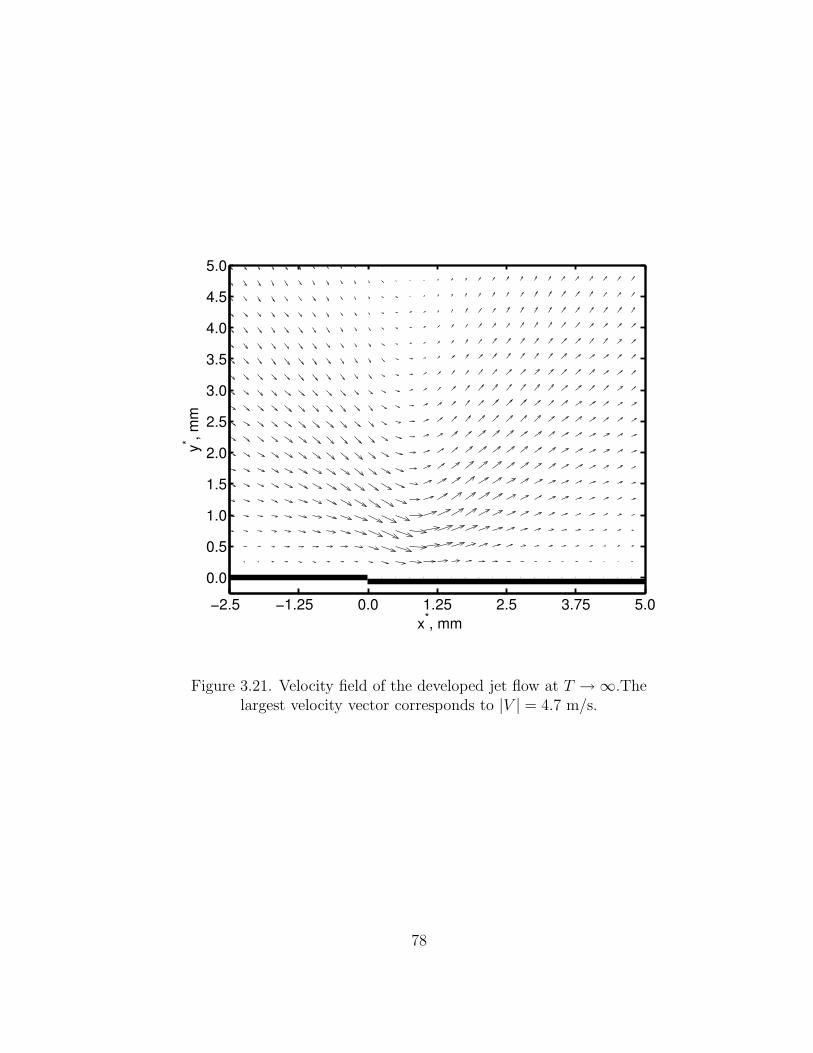
−2.5 −1.25 0.0 1.25 2.5 3.75 5.00.0
0.5
1.0
1.5
2.0
2.5
3.0
3.5
4.0
4.5
5.0
x*, mm
y* , mm
Figure 3.21. Velocity field of the developed jet flow at T → ∞.Thelargest velocity vector corresponds to |V | = 4.7 m/s.
78

Figure 3.22. Developed jet flow at T → ∞, PIV results by Post [61].
Post used a trigger signal on the PIV laser to capture the velocity field at cer-
tain time delays following the impulsive starting of the actuator. A schematic of
the laser trigger timing is shown in Figure 3.19. She then obtained ensemble aver-
ages of the velocity field generated by the impulsively started actuator. Examples
of those are shown in Figure 3.20. The actuator is located at x=−26 mm.
The experimental results correspond to time delays of 2, 12, 35 and 60 mil-
liseconds. These show the initial development of a starting vortex with counter-
clockwise circulation. As time progresses in the experiment, the starting vortex
grows in size and convects to the right in the positive x-direction.
Qualitatively the velocity field obtained in the simulation, shown in Figures
3.16 and 3.17, looks similar. The size of the spatial domain of the simulations is
approximately 6 by 6 mm. Therefore they are showing the starting vortex at a
very initial stage which is closest to the smallest experimental time delay shown
on the top plot in Figure 3.20.
79

The solution for the flow field a long time after the actuator was impulsively
started is shown in Figure 3.21. The result from the experiment of Post [61]
is shown in Figure 3.22. Both show that the flow is drawn down towards the
actuator and then accelerated away from the actuator in the direction from the
upper to the lower electrode. The size of the spatial domain of the simulation is
only about one-tenth of the experimental domain in order to focus on the region
closest to the actuator. However qualitatively at least, the vector field is very
similar, indicating that the electro-static model for the actuator body force vector
is reasonably good.
3.2.3 Flow Problem Results with Temporally-spatially weighted body force.
Looking more closely at the light intensity results from photomultiplier exper-
iments, it can be noticed that the volume of plasma at any spatial location was
very dependent on time within the a.c. cycle. For example, close to the edge of the
upper (exposed) electrode, plasma light illumination intensity increased linearly
with time in each half of the a.c. period. This is evident in the light intensity
contours that were shown in Figure 2.5. This indicates that an improved body
force model from the electro-static calculations would add a second body force
weighting that would account for the time dependence of the ionization.
The temporally-spatially weighted electro-static body force was represented by
the form
~f ∗
b (x, y) = ~f ∗
b (x, y) · w(x) · a(t) (3.71)
where w(x) is the previously defined spatial weighting function, and a(t) represents
the linear temporal growth observed in the experiments. The total space-time
80

0.01.25
2.53.75
5.0 0.0
0.25
0.50
0.5
1
t / Ta.c.x*, mm
Figure 3.23. Magnitude of the space-time weighting function used on theelectro-static body force for one half of the a.c. cycle.
weighting function , w(x) · a(t), is presented in Figure 3.23 for one half period of
the a.c. cycle.
The results of the numerical simulation for the flow generated by the actuator
on the bottom wall in a rectangular enclosure with the added temporal weighting
on the body force is qualitatively similar to previous case with only the spatial
weighting. When the actuator was impulsively started it produced a similar start-
ing vortex with counterclockwise circulation that grows in size and convects away
as before. At large solution times, the flow near the actuator again becomes a
81

−1 0 1 2 3 4 5 6x 10⁻⁴
−0.5
0
0.5
1
1.5
time, s
f b / f b,
max
Figure 3.24. Method for introducing space-time weighting ofelectro-static body force during time-steps of the Navier-Stokes solver.
steady tangential wall jet in the direction towards and away from the covered
electrode.
To compare the two cases of the two types of weighting on the body force, the
long time steady solution was considered. In particular, wall-normal profiles of the
x-component of velocity were compared. As a first step in comparing the profiles,
the distance from the actuator where the flow was self-similar was determined.
An example of this for the case with only spatial weighting for the steady (long-
time) solution is shown in Figure 3.25. Here the profiles were taken at different x
locations in the induced flow direction away from the actuator. The velocities in
the profiles were normalized by the maximum at that x-location. The wall normal
coordinate was normalized by the y-value of the velocity maximum. These are
82

defined in the following.
Unorm =U
Umax(3.72)
ynorm =y
y(Umax)
Focusing on the normalized profiles in Figure 3.25, we observe that by the
fourth location away from the actuators, the profiles begin to fall onto a single
curve. This is particularly evident in the lower part of the profiles up to the
height corresponding to Umax. Based on this result, velocity profiles for the two
body force weighting cases were compared at X = 0.5938. These are compared
at different times after the impulsive start of the actuator body force in Figures
3.26 and 3.27.
Figure 3.26 shows the velocity profiles for the case with only spatial weighting
of the body force. The profiles for the case with space-time weighting are shown
in Figure 3.27. Both of these show the character of an accelerating wall jet. The
outer part of the profile, above y∗ = 1 cm, has negative velocities due to reverse
flow produced by a flow recirculation in the box that was induced by the actuator.
One of the things that can be easily noticed on the comparison of the two cases
is that the space-time weighted body force resulted in a maximum velocity that
was approximately one-third that of the other weighting. This indicates that the
time response of the ionization is significant to the performance of the actuator.
It suggests that the performance would increase if the a.c. frequency is increased.
This is an aspect that will be examined with the lumped-element circuit model in
a section to follow.
83

−0.2 0 0.2 0.4 0.6 0.8 1 1.20
0.5
1
1.5
2
2.5
3
u* / u*max
y* / y* m
ax v
eloc
ity
X=0.2X=0.3X=0.4X=0.5X=0.6X=0.7X=0.8X=0.9X=1.0
Figure 3.25. x-component velocity profiles normalized by maximumvelocities and the locations of maximum velocities at different locationsdownstream of the simulated actuator with spatial weighting of the body
force and the steady (long-time) solution.
84
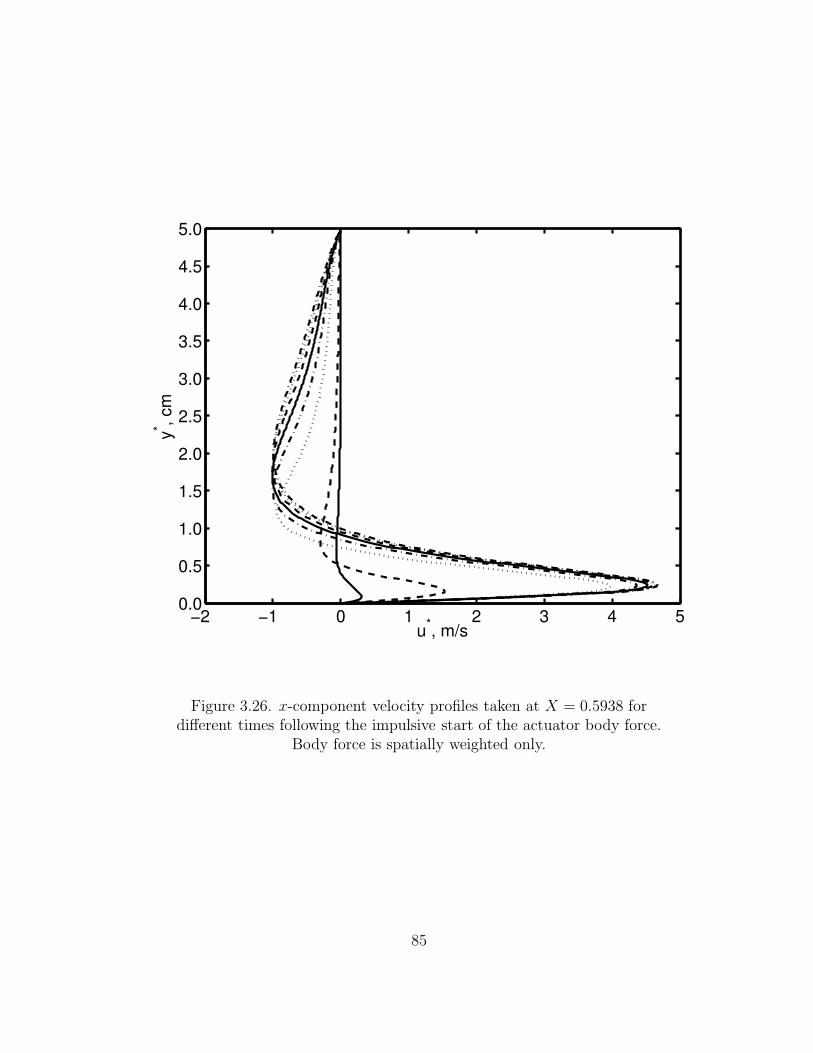
−2 −1 0 1 2 3 4 50.0
0.5
1.0
1.5
2.0
2.5
3.0
3.5
4.0
4.5
5.0
u*, m/s
y* , cm
Figure 3.26. x-component velocity profiles taken at X = 0.5938 fordifferent times following the impulsive start of the actuator body force.
Body force is spatially weighted only.
85
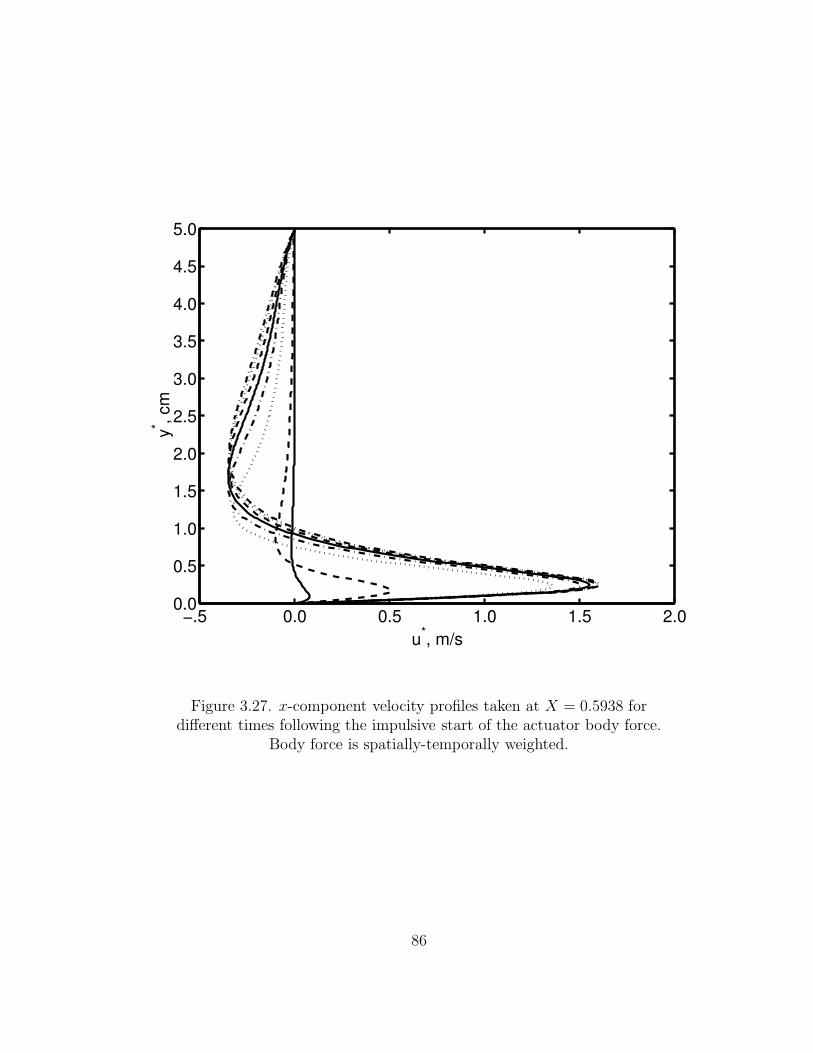
−.5 0.0 0.5 1.0 1.5 2.00.0
0.5
1.0
1.5
2.0
2.5
3.0
3.5
4.0
4.5
5.0
u*, m/s
y* , cm
Figure 3.27. x-component velocity profiles taken at X = 0.5938 fordifferent times following the impulsive start of the actuator body force.
Body force is spatially-temporally weighted.
86

0.0 0.02 0.04 0.06 0.08 0.10.0
0.5
1.0
1.5
2.0
2.5
3.0
3.5
4.0
4.5
5.0
Time, s
u* max
, m/s
spatially weightedspace−time weighted
*
*
Figure 3.28. Maximum x-component velocity as a function of time forimpulsively started actuator body force. Star indicates first-order time
constant corresponding to where UUt→∞
= 1e.
The temporal response of the flow can be characterized by its response to the
impulsive (step) start of the actuator body force. To illustrate this, the maximum
velocities form Figures 3.26 and 3.27 as a function of time were plotted in Figure
3.28. This indicates that the maximum velocity of the flow induced by the actuator
reaches an asymptote after long time. If we consider this to be a first-order
response to a step input, the time constant corresponds to the time when the
velocity is 66.3 (1/e) of the values at large time. This point has been noted by
the star symbol in the figure.
87

We observe that the time constant for the flow response is the same value
for the two initial conditions. Although these initial conditions were obtained by
using different weighting on the body force, they are essentially only different by
the amplitude of the step input. Therefore we expect the time constant to be the
same for the two trials with different initial amplitudes. The value of τ = 0.01 s
suggests a frequency response of 100 Hz. This result for the time constant value
corresponds well to the result from the experiment by Post [61].
Although the electro-static model for the plasma actuator could correctly de-
scribe its effect on a neutral ambient fluid, it cannot model the the effects of the
input voltage amplitude or a.c. frequency. The success of the simulations in this
section were due to experimentally determined ionization in space and time that
corresponds to a particular a.c. frequency and amplitude.
To illustrate the problem, if one would use the electro-static model with dif-
ferent input voltage amplitudes, the dimensionless plasma body force would be
[76]
fb = α · ϕ · ∇ϕ, (3.73)
where α is the dimensionless scaling parameter given as
α =ε0ϕ
20
ρ∞U2∞λ2
D
. (3.74)
As before ϕ0 is the amplitude of the electrode potential, U∞ is a characteristic
fluid velocity, and ρ∞ is a characteristic fluid density. Equations (3.73) and (3.74)
suggest that the plasma body force will increase quadratically with the input
voltage amplitude, namely
fb ∼ V 2app. (3.75)
88

5 6 7 8 9 10100
101
Applied voltage amplitude, kV
U max
/ U m
ax, 5
kV
electrostatic modelU ∼ V2
U ∼ V7/2
Figure 3.29. Maximum induced velocity in electro-static actuator modelas a function of voltage.
If this form of the body force is used with the flow solver, the maximum induced
velocity is found to increase in proportion to the square of the applied voltage.
This is shown in Figure 3.29, in which Umax ∼ V 2app.
The problem with this result is that it contradicts all of the experimental
observations where the thrust force produced by a plasma actuator [20] and the
maximum velocity induced by the actuator [61] were observed to increase as V7/2app .
The difference in the voltage dependence can be explained by the fact that the
electro-static model does not account for charge build-up on the surface of the
dielectric or change in the volume of the plasma produced as a function of the
89
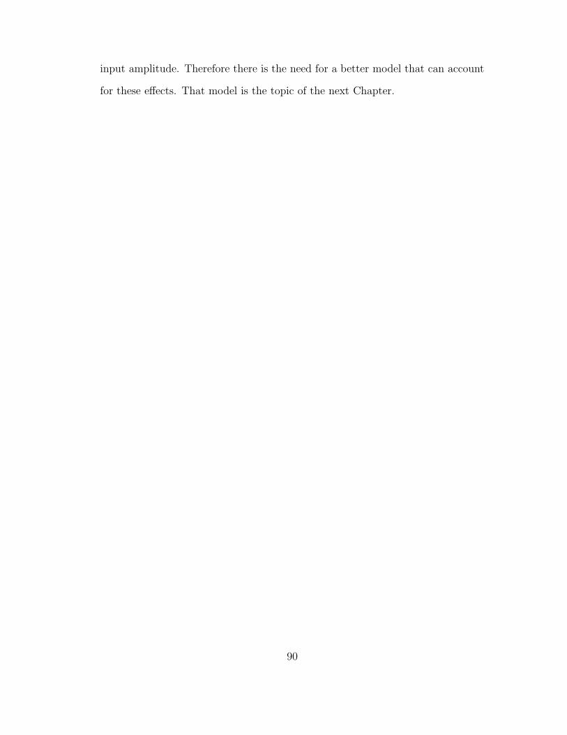
input amplitude. Therefore there is the need for a better model that can account
for these effects. That model is the topic of the next Chapter.
90

CHAPTER 4
LUMPED-ELEMENT CIRCUIT MODEL
In order to improve upon the electrostatic model for the plasma actuator pre-
sented in the previous chapter, two different lumped-element circuit models were
examined. The purpose of the lumped element circuit approach was to account
for the fact that the basic actuator configuration is a capacitive element (two elec-
trodes separated by a dielectric layer). In addition, the air is a resistive element
that has properties that depend on the degree to which it is ionized. Starting with
this basic formulation, two types of lumped-element models were considered. The
first is a temporal model with a fixed number of circuit elements. The second is
a space-time model that uses a large number of elements and can determine such
features as the plasma maximum extent and sweep velocity a priori.
4.1 Spatial Lumped-Element Circuit Model
4.1.1 Mathematical Formulation
The spatial lumped-element model uses a fixed number of circuit elements to
represent the actuator and air. This method was first suggested by Enloe [17].
The model, shown in Figure 4.1, consists of a number of capacitive elements, and
a single resistive element, representing the plasma. Each of this elements varies
91

in time as the plasma discharge evolves throughout the AC cycle of the applied
voltage.
The exposed surface of the dielectric also plays a critical role in the circuit
dynamics. Even before the air ionizes, the dielectric surface communicates the
potential charge from the covered electrode. When the voltage potential is large
enough to ionize the air, the surface of the dielectric collects or discharges addi-
tional charge. As a result we refer to the dielectric surface as a virtual electrode
in the circuit.
Three capacitances can be established in the circuit. Capacitance C1 repre-
sents the capacitance between the exposed electrode and the top surface of the
dielectric. Capacitance C2 represents the capacitance between the top surface
of the dielectric and the encapsulated electrode. Capacitance C3 represents the
capacitance between the two physical electrodes.
When the air is ionized, a portion of capacitance C1 is bypassed by the con-
ductivity of the plasma. This can be accounted for by splitting the capacitance C1
into two elements: C1A, which is bypassed when the plasma is present, and C1B,
which is not. The total capacitance remains constant throughout the discharge
cycle, namely
C1A + C1B = C1 = Const. (4.1)
The same stipulation is made for the capacitance C2.
The values of the captaincies C2A and C2B can be calculated as
C2A(t) =ε0zx(t)
d(4.2)
C2B(t) =ε0z[L− x(t)]
d, (4.3)
92
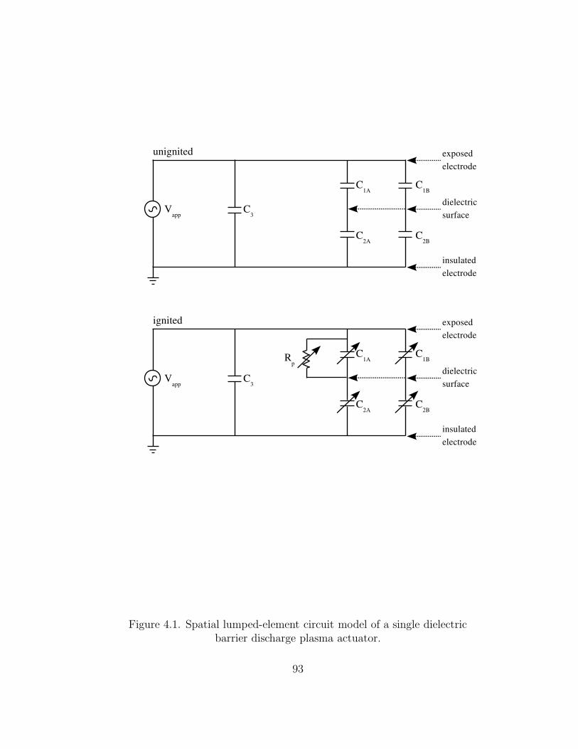
Figure 4.1. Spatial lumped-element circuit model of a single dielectricbarrier discharge plasma actuator.
93

where d is the thickness of the dielectric, z is the span-wise length of the actuator,
ε0 is the permittivity of the free space, L is the length of the encapsulated elec-
trode, and x is the extent of the plasma. Variables x, C2A and C2B are explicitly
identified as functions of time, t.
Due to the complexity of the electrode geometry, calculating the capacitances
C1A and C1B from first principles is less straightforward. But an assumption can
be made that these C1A and C1B are proportional to C2A and C2B, respectively.
Thus
C1A(t) = αC2A(t) (4.4)
and
C1B(t) = αC2B(t) (4.5)
where α is a constant that can be estimated from experiments. The capacitance
C3 is a constant that is given from the dielectric material properties and the area
of the electrodes. it is easily estimated or found from experiment.
As the plasma expands over the dielectric, its resistance drops as the conduc-
tance path becomes wider. This variable resistance can be treated in the model
by making the conductance of the plasma, Gp proportional to the extent of the
plasma namely,
Gp(t) =1
Rp(t)=
(
G0
L
)
x(t), (4.6)
where G0 is the conductance of the plasma when the plasma reaches its maximum
extent at x = xmax. The value of G0 depends on the geometry of the actuator, and
the density and the temperature of the plasma. The conductance of the plasma
can be measured in the experiment.
94
Figure 4.2. Schenatic showing three node points where voltage isfollowed in the circuit in the spatial lumped-element circuit model of a
single dielectric barrier discharge plasma actuator.
To implement the model, it is necessary to follow the voltage at three node
points in the circuit as shown in Figure 4.2: the applied voltage Vapp, which appears
across the entire network, the voltage at the virtual electrode covered by plasma
which is designated as V2A, and the voltage at the virtual electrode not covered
by plasma which is designated as V2B . Due to the presence of the capacitances in
the circuit, it is necessary to define the applied voltage Vapp in terms of its time
derivative. In the case of a simple sinusoidal input, this is
dVapp(t)
dt= V0ω cos(ωt), (4.7)
where V0 is the amplitude of the applied voltage and ω is its angular frequency.
The capacitance C2B is charged and discharged by the displacement current
flowing through the capacitance C2A. The voltage across capacitor C2B is V2B
which is governed by
dV2B(t)
dt=dVapp(t)
dt
(
C1B(t)
C1B(t) + C2B(t)
)
. (4.8)
95

The voltage at the virtual electrode covered by the plasma discharge is given by
dV2A(t)
dt=dVapp(t)
dt
(
C1A(t)
C1A(t) + C2A(t)
)
+Ip(t)
C1A(t) + C2A(t). (4.9)
This includes the real current through the plasma which is proportional to the
plasma’s conductance, G. The current flowing through the plasma is given as
Ip(t) = Gp(t) [Vapp(t) − V2A(t)] . (4.10)
Starting from the moment of air ionization, the extent of spreading of the plasma
over the dielectric covering of the lower electrode is given as
dx(t)
dt= νV |Vapp(t) − V2A(t)| , (4.11)
where νV is the coefficient representing the increase in the sweep velocity with the
increase in applied voltage amplitude. The proportionality factor νV is empirically
determined from experiments. In the present work, νV = 10m/skV
as seen in Figure
2.6. Because velocity of the plasma edge involves the absolute value of the voltage
difference across the plasma, the plasma expands in essentially the same way
regardless of the polarity of the ionization.
By solving the system of equations given by equations (4.7) through (4.11),
the voltages at each node in the circuit, and the physical extent of the plasma
can be determined as function of time. Examples of these and the sensitivity they
have on some of the empirically determined variables are presented in the next
section.
96

4.1.2 Numerical Formulation of Temporal Lumped-Element Circuit Model
The governing equations of the lumped-element circuit model, given by equa-
tions (4.9), (4.9) and (4.10), can be rewritten as
dV2B(t)
dt=
dVapp(t)
dt
(
C1B(t)
C1B(t) + C2B(t)
)
, (4.12)
dV2A(t)
dt=
dVapp(t)
dt
(
C1A(t)
C1A(t) + C2A(t)
)
+Gp(t) [Vapp(t) − V2A(t)]
C1A(t) + C2A(t).
From the first equation, the value of V2B can be evaluated directly since the values
of the capacitances are known at the time step t. The second equation is the initial
value problem, which can be written in a more general case of a first-order ordinary
differential equation as
dV2A
dt= f(t, V2A). (4.13)
This initial value problem is solved using the standard IMSL routine IVPAG which
implements the Adams-Moultons’s method [1].
For this IVPAG routine, the time interval was specified along with the initial
values of the voltage V2A. As a solution we get the value of the voltage at the next
time step.
The numerical procedure consists of the following steps:
1. Specify initial values for the temporal lumped-element circuit model at time
t = 0;
2. Compute the voltage difference across the actuator, compare the value to
the plasma ignition threshold value which determines the plasma presence
on the dielectric surface;
97
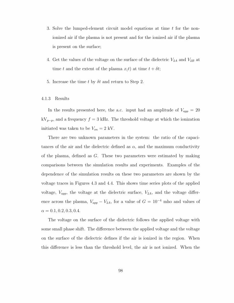
3. Solve the lumped-element circuit model equations at time t for the non-
ionized air if the plasma is not present and for the ionized air if the plasma
is present on the surface;
4. Get the values of the voltage on the surface of the dielectric V2A and V2B at
time t and the extent of the plasma x(t) at time t+ δt;
5. Increase the time t by δt and return to Step 2.
4.1.3 Results
In the results presented here, the a.c. input had an amplitude of Vapp = 20
kVp−p, and a frequency f = 3 kHz. The threshold voltage at which the ionization
initiated was taken to be Von = 2 kV.
There are two unknown parameters in the system: the ratio of the capaci-
tances of the air and the dielectric defined as α, and the maximum conductivity
of the plasma, defined as G. These two parameters were estimated by making
comparisons between the simulation results and experiments. Examples of the
dependence of the simulation results on these two parameters are shown by the
voltage traces in Figures 4.3 and 4.4. This shows time series plots of the applied
voltage, Vapp, the voltage at the dielectric surface, V2A, and the voltage differ-
ence across the plasma, Vapp − V2A, for a value of G = 10−4 mho and values of
α = 0.1, 0.2, 0.3, 0.4.
The voltage on the surface of the dielectric follows the applied voltage with
some small phase shift. The difference between the applied voltage and the voltage
on the surface of the dielectric defines if the air is ionized in the region. When
this difference is less than the threshold level, the air is not ionized. When the
98
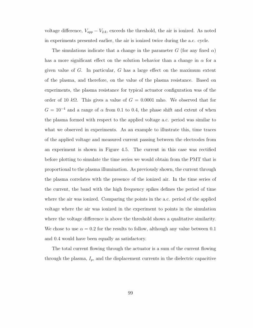
voltage difference, Vapp − V2A, exceeds the threshold, the air is ionized. As noted
in experiments presented earlier, the air is ionized twice during the a.c. cycle.
The simulations indicate that a change in the parameter G (for any fixed α)
has a more significant effect on the solution behavior than a change in α for a
given value of G. In particular, G has a large effect on the maximum extent
of the plasma, and therefore, on the value of the plasma resistance. Based on
experiments, the plasma resistance for typical actuator configuration was of the
order of 10 kΩ. This gives a value of G = 0.0001 mho. We observed that for
G = 10−4 and a range of α from 0.1 to 0.4, the phase shift and extent of when
the plasma formed with respect to the applied voltage a.c. period was similar to
what we observed in experiments. As an example to illustrate this, time traces
of the applied voltage and measured current passing between the electrodes from
an experiment is shown in Figure 4.5. The current in this case was rectified
before plotting to simulate the time series we would obtain from the PMT that is
proportional to the plasma illumination. As previously shown, the current through
the plasma correlates with the presence of the ionized air. In the time series of
the current, the band with the high frequency spikes defines the period of time
where the air was ionized. Comparing the points in the a.c. period of the applied
voltage where the air was ionized in the experiment to points in the simulation
where the voltage difference is above the threshold shows a qualitative similarity.
We chose to use α = 0.2 for the results to follow, although any value between 0.1
and 0.4 would have been equally as satisfactory.
The total current flowing through the actuator is a sum of the current flowing
through the plasma, Ip, and the displacement currents in the dielectric capacitive
99
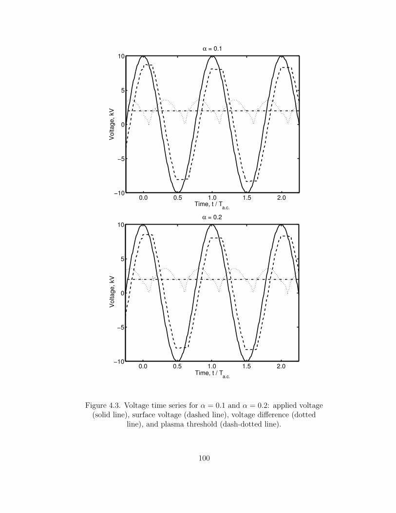
0.0 0.5 1.0 1.5 2.0−10
−5
0
5
10
Time, t / Ta.c.
Volta
ge, k
V
α = 0.1
0.0 0.5 1.0 1.5 2.0−10
−5
0
5
10
Time, t / Ta.c.
Volta
ge, k
V
α = 0.2
Figure 4.3. Voltage time series for α = 0.1 and α = 0.2: applied voltage(solid line), surface voltage (dashed line), voltage difference (dotted
line), and plasma threshold (dash-dotted line).
100

0.0 0.5 1.0 1.5 2.0−10
−5
0
5
10
Time, t / Ta.c.
Volta
ge, k
V
α = 0.3
0.0 0.5 1.0 1.5 2.0−10
−5
0
5
10
Time, t / Ta.c.
Volta
ge, k
V
α = 0.4
Figure 4.4. Voltage time series for α = 0.3 and α = 0.4: applied voltage(solid line), surface voltage (dashed line), voltage difference (dotted
line), and plasma threshold (dash-dotted line).
101

0 1 2
−1.5
−1.0
−0.5
0.0
0.5
1.0
1.5
2.0
t / Ta.c.
Appl
ied
volta
ge, k
V
Voltage
I ⋅ 105 (A)
Figure 4.5. Applied voltage and rectified current in the circuit,experimental results.
102

element. This is given as
Itotal = Ip +d(C1U1A)
dt+d(C2U2A)
dt+ C3
dVapp
dt. (4.14)
The current flowing through the plasma was given by Equation (4.10). We note
that the displacement currents in the dielectric capacitor elements are several
orders of magnitude smaller than Ip. This current will be used to determine the
power dissipated by the plasma.
The plasma is the only dissipative element in the circuit. Due to this, the
instantaneous power P (t) is given as
P (t) = Ip(t) |Vapp(t) − V2A(t)| . (4.15)
The average dissipated power as a function of the applied voltage is shown
in Figure 4.6. This is plotted on log axes to illustrate the power law relation
between the dissipated power and voltage. Except for the lowest voltage, the
dissipated power is proportional to the applied voltage to the 7/2 power. This is
consistent with actuator thrust measurements by Enloe [20] and induced velocity
measurements from Post [61] that both showed a 7/2 power-law dependence with
the applied voltage.
The total volume of plasma is proportional to the plasma extent, x(t). The
dependence of the plasma extent on the input voltage amplitude has been exam-
ined in the previously discussed experiments. Model simulations were performed
for a range of voltage from 10 kVp−p to 40 kVp−p. Figure 4.8 shows the model
predictions for maximum extent of the plasma.Shown for comparison are the ex-
perimental values from our experiment and from Enloe et al. [20]. All agree
103

4 8 12 16 20
0.05
0.1
0.5
1
Vp−p, kV
Diss
ipat
ed P
ower
: ∫P /
∫Pm
ax
V7/2
Figure 4.6. Average dissipated power as a function of the applied voltagebased on the actuator model.
104

4 8 12 16 20
0.05
0.1
0.5
1
U / U
max
Vp−p, kV
U=1.8x10⁻³ V7/2 (experiment)Power (simulation)
4 8 12 16 20
0.05
0.1
0.5
1
Diss
ipat
ed P
ower
: ∫P /
∫Pm
axFigure 4.7. Dependence of plasma actuator maximum induced velocity(open symbols) and plasma dissipated power based on lumped-element
circuit model(closed symbols as a function of applied a.c. voltage.
105

5000 10000 15000 200000
2
4
6
8
10
12
14
16
Applied voltage peak−to−peak, V
Max
imum
ext
ent o
f the
pla
sma,
mm
experiment, Orlovexperiment, Enloetemporal lumped−element circuit model
Figure 4.8. Maximum extent of the plasma as function of appliedvoltage amplitude for temporal lumped-element circuit model simulation
and experiments (Enloe [20] and present).
reasonably well. They indicate that the maximum extent increases linearly with
the applied voltage at a rate of approximately 1.25 mm/kV. This is important
because it has been show by Enloe et al. [20] that the thrust of the actuator was
limited if sufficient area of the covered electrode was not provided. That minimum
area is a function of the voltage.
The present model was successful at estimating the effect of voltage amplitude
on the body force and power dissipated by the plasma. In particular, the voltage
106

dependence of the body force was found to agree with the experimental observa-
tions by Enloe [20] and Post [61]. A shortcoming of the model was that it needed
some empirically determined coefficients that were shown in experimental results
presented in Chapter 2, to be functions of frequency. Thus the present model is
only valid for the single frequency. Although, it might be possible to modify this
model to include a broader set of coefficients, the desire was to develop a model
that embodies more of the physics of the DBD process without the need of ex-
perimental coefficients. The attempt at that model which we term the space-time
lumped-element model, is presented in the next section.
4.2 Spatial-Temporal Lumped-Element Circuit Model
4.2.1 Mathematical Formulation
As it has been shown previously, the spatial lumped-element circuit model
correctly describes many of the characteristics of the SDBD plasma actuator. By
comparisons with experimental results, it was shown that the model predicts that
the power dissipated in the plasma resistive element increases with the 7/2 power
of the applied voltage. This correlates with the experimental results by Enloe et
al. [20] and Post [62] that showed that thrust and maximum velocity generated
by the asymmetric electrode arrangement of the SDBD plasma actuator varied as
V7/2app .
Despite all the advantages of the earlier model, it had a significant limitation
in that the dynamics of the ionization relied on empirical coefficients that were
functions of the applied voltage amplitude and frequency. Therefore the model
was not able to predict the actuator dependence outside its empirical calibration
space.
107

Figure 4.9. The physical space over the encapsulated electrode is dividedinto N sub-regions.
The space-time lumped-element circuit model presented here is intended to
model the details of of the ionization process to provide predictions of the body
force for a range of parameters without the need of experimental calibration. The
space-time lumped-element model follows from the previous model in that the
air and dielectric are represented as a network of resistors and capacitors. The
difference comes in that rather than being represented by a single parallel network,
the domain over the covered electrode is divided into N parallel networks, such as
illustrated in Figure 4.9. The characteristics of each parallel network depend on its
distance from the exposed electrode. For example, parallel network 1 is closest to
the exposed electrode and extends the shortest distance over the covered electrode.
Parallel network N extends the farthest distance over the covered electrode.
Each parallel network consists of an air capacitor, a dielectric capacitor, and
a plasma resistive element as in the previous model. In addition to these, zener
diodes were added to set the threshold voltage levels at which the plasma initi-
ates, and to switch in the different plasma resistance values based on the current
108

Figure 4.10. Electric circuit model of a single dielectric aerodynamicplasma actuator.
direction, namely from the exposed electrode to the dielectric, or from the dielec-
tric to the exposed electrode, that experiments have shown to be important. The
N-circuit arrangement is shown in Figure 4.10.
The value of the air capacitor in the n-th sub-circuit is based on its distance
from the edge of the exposed electrode. This is given by equation (4.16)
Can =ε0εaAn
ln(4.16)
where εa is the dielectric coefficient of air, ln is the representative distance over the
dielectric surface, and An is the cross section of this air capacitor. The crossection
An is the product of the span-wise size of the actuator, zn, and the height of
the capacitive element, hn. The schematic of this capacitive element is shown in
Figure 4.11.
109

Figure 4.11. Schematic drawing of the n-th air capacitor.
The resistance value in the n-th sub-circuit is similarly based on its distance
from the exposed electrode. It is given by equation (4.17)
Rn =ρalnAn
(4.17)
where ρa is the effective resistivity of the air.
The value of the dielectric capacitor for each sub-circuit is similar to the air
capacitance except that it is based on the properties of the dielectric material. It
is given by equation (4.18)
Cdn =ε0εdAd
ld(4.18)
where εd is the dielectric coefficient of the dielectric material, ld is the thickness
of this material, and An is the cross section which is equal to the product of
the span-wise size of the actuator, zn, and the width of the dielectric capacitive
element, dn, as shown in Figure 4.12.
110
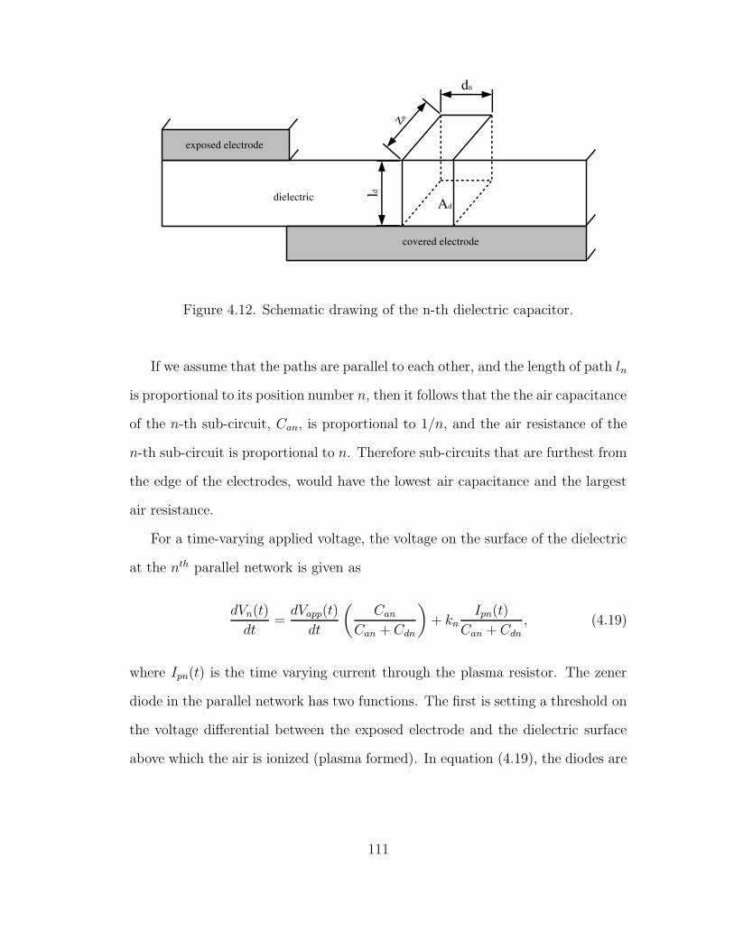
Figure 4.12. Schematic drawing of the n-th dielectric capacitor.
If we assume that the paths are parallel to each other, and the length of path ln
is proportional to its position number n, then it follows that the the air capacitance
of the n-th sub-circuit, Can, is proportional to 1/n, and the air resistance of the
n-th sub-circuit is proportional to n. Therefore sub-circuits that are furthest from
the edge of the electrodes, would have the lowest air capacitance and the largest
air resistance.
For a time-varying applied voltage, the voltage on the surface of the dielectric
at the nth parallel network is given as
dVn(t)
dt=dVapp(t)
dt
(
Can
Can + Cdn
)
+ knIpn(t)
Can + Cdn, (4.19)
where Ipn(t) is the time varying current through the plasma resistor. The zener
diode in the parallel network has two functions. The first is setting a threshold on
the voltage differential between the exposed electrode and the dielectric surface
above which the air is ionized (plasma formed). In equation (4.19), the diodes are
111

represented by the variable kn. When the threshold voltage is exceeded, kn = 1.
Otherwise kn = 0.
The second function of the zener diodes was to switch in either one of the re-
sistances representing the plasma resistance based on the direction of the current,
from the exposed electrode to the dielectric surface or vice versa. This is meant
to represent the experimental observations that the current and corresponding
plasma illumination were different based on the current direction. The resistance
values are designated as Rnf or Rnb (representing forward or backward going cur-
rent). The ratio of the two plasma resistances used in the simulation wereRnf
Rnb= 5.
This was based on the difference in the estimated current observed in experiments.
With this background, the current through the plasma resistance, Ip(t) is given
as
Ipn(t) =1
Rn[Vapp(t) − Vn(t)] . (4.20)
where Rn = Rnf or Rnb based on the current direction.
This space-time formulation of the lumped-element circuit model has many
advantages over the previous model. One advantage is that it allows us to specify
the number of the sub-circuits N making up the actuator. Ideally, as N → ∞, the
numerical solution should approach the asymptotic solution. As the tests of the
code showed, values of N ≈ 102 appear to be sufficient to capture the essential
physics. This is shown in Figure 4.13.
A second advantage of this formulation is that it is temporal. Therefore the
effect of the a.c. frequency or wave form can be examined. Dynamics such as the
sweep-out velocity of the plasma can then be determined a priori.
112

10 20 50 70 100 150 2000.999
0.9995
1
1.0005
1.001
Number of parallel networks
max
( f b /
f b ∞ )
Figure 4.13. Maximum value of the plasma body force as function of thenumber of parallel networks.
113

4.2.2 Numerical Formulation of Space-Time Lumped-Element Circuit Model
The governing equations of the lumped-element circuit model, given by equa-
tions (4.19) and (4.20), can be rewritten as
dVn(t)
dt=dVapp(t)
dt
(
Can
Can + Cdn
)
+ kn
1Rn
[Vapp(t) − Vn(t)]
Can + Cdn. (4.21)
This is a typical initial value problem, and it can be written in general form as
dVn
dt= f(t, Vn), (4.22)
or as a finite difference equation
δVn = f(t, Vn)δx (4.23)
This equation is is solved using the standard Runge-Kutta 45 method. In this
method, we made two mid-point derivative evaluations, which led us to the fol-
lowing equations:
k1 = δtf(tm, V mn ),
k2 = δtf(tm +1
2δt, V m
n +1
2k1),
k3 = δtf(tm +1
2δt, V m
n +1
2k2), (4.24)
k4 = δtf(tm +1
2δt, V m
n +1
2k3),
(4.25)
114
and the voltage on the next time step can be calculated from the previous time
step using the following equation
V m+1n = V m
n +k1
6+k2
3+k3
3+k4
6+O(∆t5). (4.26)
This method is implemented using the standard MATLAB function ode45 [5].
In MATLAB the Runge-Kutta routine uses a variable, continuously adjusted time
step. The adaptive time-stepping algorithm takes small steps where the function
is changing rapidly and can take really big time steps where the function is smooth
and not varying much.
For the initial conditions at t = 0 we took Vn = 0 on the surface of the
dielectric. On each of the next time steps the initial conditions on Vn were taken
from the solution on the previous time step.
Thus, the procedure consists of the following step.
1. Calculate the values of resistances and capacitances in each of the parallel
networks;
2. Specify initial values of the voltage on the dielectric surface at time t = 0;
3. Specify the time step δt;
4. Specify the time interval: [t, t+ δt];
5. Solve the ODE given by equation (4.21) using the ode45 routine in MATLAB
on the specified time interval;
6. Check for the plasma presence in all the parallel networks, if the plasma
is present in the n-th network, set the plasma presence coefficient kn = 1,
115

if the threshold for the plasma ignition is not reached in the n-th parallel
network, then set kn = 0;
7. Calculate the plasma current and set the resistance of the plasma depending
on the direction of the plasma current;
8. Reinitialize the initial values of the voltage on the surface for the ODE solver
solution on this time step;
9. Increase time by δt;
10. Return to Step 4.
4.2.3 Results of Space-Time Lumped-Element Circuit Model
As an example, the electric circuit equations (4.19) were solved for 100 parallel
circuit elements making up a SDBD actuator. For this, the applied voltage was
a sine wave with amplitude of 5 kVp−p, and a frequency of 5000 Hz. In order to
resolve the dynamic motions of the plasma, a computational time step of 8 · 10−7
seconds was used. This corresponded to 250 time steps within each cycle of the
a.c. input period.
The solution of the model equations gives the voltage on the surface of the
dielectric, Vn, for each parallel circuit element. An example of this for the first
five circuit elements, closest to the exposed electrode, is shown in Figure 4.14.
We observe that there is a shift in time of the peak voltage in successive current
elements. This reflects the sweep out of the plasma over the dielectric surface.
Figure 4.15 shows the time series in the current through the first five circuit
elements in the model. Plasma is formed where the current is non-zero. This
is observed to occur twice per a.c. period at the time periods when the voltage
116

0.0 0.5 1.0 1.5
−2.0
−1.0
0.0
1.0
2.0
t / Ta.c.
Volta
ge, k
V
Vappn=1n=2n=3n=4n=5
Figure 4.14. Voltage on the surface of the dielectric in the first fivesub-circuits (n=1,2,3,4,5) obtained from space-time lumped element
circuit model.
difference between the exposed electrode and dielectric surface exceeds a threshold
level. Again we observe that the time when the plasma first forms increases as
the sub-circuit is further from the exposed electrode. As with the voltage, this
reflects the sweep out of the plasma during the input a.c. cycle.
It may be noticed that the plasma current is not symmetric during the a.c.
cycle - the current going through the plasma resistive elements is larger during
one half of the cycle than the current going in the opposite direction during the
other half of the cycle. But the total current in the circuit is the sum of the real
117

0.0 0.5 1.0 1.5−1
0
1
2
3
4
5 x 10⁻⁵
t / Ta.c.
Curre
nt, A
n=1n=2n=3n=4n=5
Figure 4.15. Plasma current in the first five sub-circuits (n=1,2,3,4,5)obtained from space-time lumped element circuit model.
118

and displacement currents in the parellel networks, and it can be written as
Itotal(t) =N∑
n=1
(
Ipn(t) +d(Cna(Vapp(t) − Vn(t)))
dt
)
. (4.27)
The charge transfered through the circuit is given by
Qtotal =
∫ 1
t=0
Itotal(t)dt. (4.28)
Integrating the total current for one a.c. period, as given by Equations (4.27) and
(4.28), we get
Qtotal = 0. (4.29)
This results signifies the conservation of charge in the system.
As has been noted previously in the experiments, the electric current in the
plasma relates directly to the light emission from the SDBD, and thus is an indi-
cation of the volume of the plasma. Therefore to compare to the experiments, the
rectified plasma current from the model in time and space above the dielectric-
covered electrode is shown in Figure 4.16. Zero on the space axis corresponds
to the edge of the exposed electrode. The time axis is shown as a fraction of
the input a.c. period. This can be directly compared to Figure 2.4 that showed
the space-time variation of the plasma illumination. The rectified current from
the model is very similar to the experimental result. It clearly shows the largest
current at the edge of the exposed electrode and the rapid decay when moving
away from electrode’s edge. In addition, the model simulates ionization occurring
twice during the a.c. cycle, and the difference in the magnitude of the current in
the two halves of the cycle.
119

Figure 4.16. Rectified plasma current for one a.c. period of inputobtained from space-time lumped element circuit model.
120

0 50 100
0.5
1.0
position over dielectricin % of covered electrode
t / T
a.c.
0.1
0.90.8 0.7 0.6 0.5 0.1
Figure 4.17. Contour lines of constant rectified plasma current obtainedfrom space-time lumped element circuit model.
The same result shown in Figure 4.16 is plotted in Figure 4.17 as contour lines
of the constant plasma current. This again illustrates the good agreement between
the model and the photomultiplier experiments shown in Figure2.5.
The results from the photomultiplier experiments and from the space-time
lumped-element circuit model can be compared quantitatively. There are two
important characteristics of the plasma discharge that can be extracted from this
data. The first is the maximum extent of the plasma over the surface of the
dielectric. The results from the model and experiments are show in Figure 4.18.
121

Also included in the figure are experimental results from Enloe et al. [21]. The
figure shows the extent of the plasma as a function of the peak-to-peak voltage.
First, we notice that the plasma extent varies varies approximately linearly with
the input voltage. Second, we observed very good agreement between the model
results and the experimental results. The agreement with our experiment is better
because the model used a dielectric coefficient for PC board material (glass-epoxy)
which was used in our experiments. The experiments by Enloe et al. [21] used
Kapton film which has a different dielectric coefficient and thickness.
This result is very important for the design of plasma actuator. Post [61] noted
that at higher voltages, if the width of the covered electrode was too small, the
magnitude of the induced velocity would asymptote. A similar result was found
for the thrust produced by the actuator in experiments by Enloe et al. [21].
Another distinctive feature that can be compared is the sweep out velocity.
This corresponds to the space-time slope of the outer edge of the light intensity
contours. A comparison for the plasma sweep velocity between the space-time
simulations and plasma illumination experiments are shown in Figure 4.19. Also
included in the figure are results from the experiments of Enloe et al. [21]. The
simulation shows that the plasma sweep velocity increases slightly with the applied
voltage amplitude. The agreement with the experiment is very good. The range
of sweep velocities is from 75 to 110 m/s.
Another set of numerical simulation has been performed to study the depen-
dence of the major plasma characteristics, such as the maximum plasma extent
over the surface of the dielectric and the plasma sweep velocity, on the applied a.c.
frequency. These results were again compared to the experimental results. The
comparison between the experimental results and the space-time lumped-element
122

5000 6000 7000 8000 90000
2
4
6
8
10
12
Applied voltage peak−to−peak, V
Max
imum
ext
ent o
f the
pla
sma,
mm
experiment, present workexperiment, Enloesimulation, present work
Figure 4.18. Comparison between space-time model and experiments forthe maximum plasma extent over covered electrode as function of
voltage.
123

5000 6000 7000 8000 90000
50
100
150
Applied voltage, V
Plas
ma
prop
ogat
ion
velo
city,
m/s
experiment, present workexperiment, Enloenumerical simulation, present work
Figure 4.19. Comparison between space-time model and experiment forplasma sweep velocity as function of voltage.
124

5 6 7 8 9 10 110
2
4
6
8
10
12
Applied a.c. frequency, kHz
Max
imum
ext
ent o
f pla
sma,
mm
experimentsimulation
Figure 4.20. Comparison between space-time model and experiment formaximum extent of the plasma as function of applied a.c. frequency.
circuit model simulation are presented in Figures 4.20 and 4.21. As it can be seen
in these figures, the model predicts that the maximum plasma extent over the
encapsulated electrode does not increase with the increasing a.c. frequency. This
also means that the plasma propagation velocity would increase linearly with the
applied frequency. This is consistent with the experimental observations. The
results obtained from the numerical simulation for the plasma sweep velocity are
in the range of 75-200 m/s and match the experimental result very well.
125

5 6 7 8 9 10 110
50
100
150
200
250
Applied a.c. frequency, kHz
Plas
ma
swee
p ve
locit
y, m
/s
experimentsimulation
Figure 4.21. Comparison between space-time model and experiment forplasma sweep velocity as function of applied a.c. frequency.
126

These results are necessary to obtain the plasma body force. The solution for
the voltage on the surface of the dielectric serves as the time-dependent boundary
condition of the electric potential, ϕ, in the electrostatic equation (4.30) at the
electrodes. The extent of the plasma on the surface of the dielectric specifies
the region of the presence of charges above the encapsulated electrode, as shown
in Figure 4.22. The value of the electric potential on the exposed electrode are
specified to be the applied voltage Vapp(t). The boundary conditions at the outer
boundaries are set to the “infinity” boundary conditions (ϕ = 0). With these
boundary conditions, the electrostatic equation
∇(ε∇ϕ) =1
λ2D
ϕ (4.30)
is solved as previously described in Chapter 2. This is done at each time step
of the lumped-element circuit model to account for the time dependence of the
ionization. The solution of the electrostatic equation is then used to calculate the
time-dependent body force produced by the plasma, given as before as
~f ∗
b = ρc~E = −
(
ε0
λ2D
)
ϕ~E. (4.31)
The procedure for the body force computation then consists of the following
steps:
1. Specify initial values for the Lumped-element Circuit Model at time t;
2. Solve the Lumped-element Circuit Model equations at time t;
3. Get the values of the voltage on the surface of the dielectric Vn at time t
and the extent of the plasma xp at time t;
127

Figure 4.22. Computational domain for calculation of unsteady plasmabody force.
128

4. Set the boundary conditions for the electric potential on the dielectric sur-
face “virtual electrode” equal to the voltage values Vn, and for the electric
potential on the upper electrode equal to the applied voltage Vapp;
5. Define the region of the charges presence over the surface of the dielectric
between the junction of the electrodes and the extent of the plasma xp;
6. Solve the electrostatic equation for the electric potential ϕ as described in
Chapter 3;
7. Calculate the plasma body force ~fb at time t as described in Chapter 3;
8. Increase the time t by δt and return to Step 1.
Following this procedure, an example of the normalized magnitude of the
plasma body force for the asymmetric electrode arrangement illustrated in Figure
4.22 is shown in Figure 4.23. This shows the body force distribution in space and
time. It can be noticed that the largest magnitude of the plasma body force is
near the edge of the exposed electrode. From that location the magnitude decays
rapidly over the surface of the dielectric. Recall that experiments indicated that
the plasma illumination decreased exponentially. This is consistent with the de-
cay that comes from the solution of the lumped-element circuit model. It justifies
the exponential weighting that was used in the electrostatic model described in
Chapter 3.
Another feature that can be noticed from Figure 4.23 is that the body force
peaks four times during one a.c. cycle. This is clearly seen in Figure 4.24 where
the maximum value of the body force near the edge of the electrode is plotted as
a function of time for one a.c. period. The fact that the body force has four peaks
is resulting from the body force formulation (4.31) and the fact that during the
129
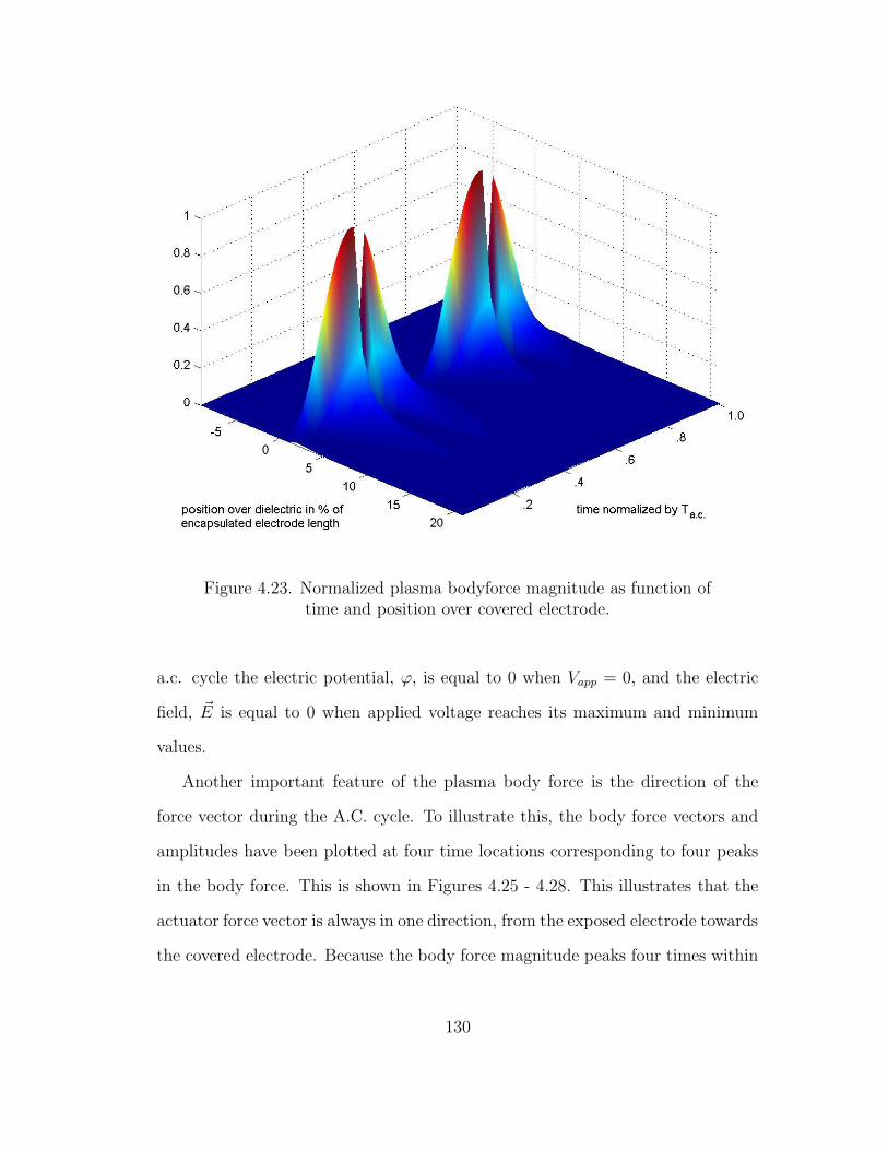
Figure 4.23. Normalized plasma bodyforce magnitude as function oftime and position over covered electrode.
a.c. cycle the electric potential, ϕ, is equal to 0 when Vapp = 0, and the electric
field, ~E is equal to 0 when applied voltage reaches its maximum and minimum
values.
Another important feature of the plasma body force is the direction of the
force vector during the A.C. cycle. To illustrate this, the body force vectors and
amplitudes have been plotted at four time locations corresponding to four peaks
in the body force. This is shown in Figures 4.25 - 4.28. This illustrates that the
actuator force vector is always in one direction, from the exposed electrode towards
the covered electrode. Because the body force magnitude peaks four times within
130

0.0 0.5 1.00
0.5
1
Time, normalized by Ta.c.
max
| f b |
, nor
mal
ized
by |
f b,m
ax |
Figure 4.24. Normalized maximum value of the plasma bodyforcemagnitude as function of time. Dots indicate where the snapshots of the
body force vector fields are taken.
131

−5.08 0.0 5.080.0
1.14
x, mm
y, m
m
−5.08 0.0 5.08
0.0
0.5
1.0
x, mm
| fb |
Figure 4.25. Plasma body force vector field and body force amplitude att = 0.2 · Ta.c.. The body force is normalized by the maximum value in
the a.c. cycle.
the a.c. period and two of the peaks are slightly smaller this might be represented
as “Push-push-Push-push” for one a.c. period
These observations suggest that the spectral analysis of the body force may
reveal important features of the plasma discharge and also serve as a tool for
comparison with the experimental data. For example, the spectrum results can
be directly compared to the acoustic or accelerometer measurements of the plasma
actuator [57].
132

−5.08 0.0 5.080.0
1.14
x, mm
y, m
m
−5.08 0.0 5.08
0.0
0.5
1.0
x, mm
| fb |
Figure 4.26. Plasma body force vector field at t = 0.4 · Ta.c.. The bodyforce is normalized by the maximum value in the a.c. cycle.
133

−5.08 0.0 5.080.0
1.14
x, mm
y, m
m
−5.08 0.0 5.08
0.0
0.5
1.0
x, mm
| fb |
Figure 4.27. Plasma body force vector field at t = 0.7 · Ta.c.. The bodyforce is normalized by the maximum value in the a.c. cycle.
134

−5.08 0.0 5.080.0
1.14
x, mm
y, m
m
−5.08 0.0 5.08
0.0
0.5
1.0
x, mm
| fb |
Figure 4.28. Plasma body force vector field at t = 0.9 · Ta.c.. The bodyforce is normalized by the maximum value in the a.c. cycle.
135
We performed the spectral analysis of the plasma body force signal shown
previously in Figure 4.24. The resulting spectrum is shown in Figure 4.29. it can
be noticed that the dominating frequency in this spectrum is twice the frequency
of the plasma actuator. This result is consistent with the body force signal shown
in Figure 4.24 where the both peaks of the body force are approximately equal.
This domination of the second harmonic was also noticed in the experiments by
Porter et al. [57]. In their experiment, the spectrum of the accelerometer signal
showed the dominance of the second harmonic in one of the studied cases (7 kHz),
but not in the other two cases (5 and 6 kHz). This difference in their observations
may be explained by the transfer to the filamentary regime at lower frequencies
when the plasma becomes non-uniform.
Using the space-time lumped-element circuit model we were able to study the
effect that different dielectric materials had on the plasma body force. Three
different materials were tested with the dielectric coefficients ε = 10, 100, and
1000. A set of numerical simulations has been carried out for a range of a.c.
frequencies from 1 Hz to 10 kHz. The results of these simulations are presented
in Figures 4.30 and 4.31 for the plasma body force and the power dissipated by
the actuator.
From the body force results we notice that for each material tested there exists
the optimal frequency at which the plasma actuator output is maximum in terms
of the force produced. This result is consistent with the general theory of the
RC circuits. On the other hand, it has been noticed that the dissipated power
increases with the a.c. frequency, and reaches its maximum values at high a.c.
frequencies. This suggested that at the higher a.c. frequencies this power does
not turn into the body force any more. Instead, it goes into the ohmic heating.
136

0 2 4 6 8 100
0.2
0.4
0.6
0.8
1
f / fact
F’b
Figure 4.29. Spectrum of the plasma body force obtained withspace-time lumped-element circuit model.
137

1 10 100 1000 100000
0.1
0.2
0.3
0.4
0.5
0.6
0.7
0.8
0.9
1
Applied frequency, Hz
Norm
alize
d bo
dy fo
rce,
f b / f b,
max
ε=10ε=100ε=1000
Figure 4.30. Effect of dielectric material on plasma body force.
The other interesting feature that can be noticed here is that the optimum
frequency of the plasma actuator depends on the dielectric properties of the ma-
terial, and decreases with the increasing dielectric coefficient. Our simulations
showed that it shifts from the kHz range to the Hz range for ε changing from 10
to 1000.
The space-time lumped-element circuit model showed excellent agreement with
the experimental results. It allowed us to calculate the time-dependent volume of
the plasma over the electrodes during the a.c. cycle. It also provided an efficient
138

1 10 100 1000 100000
10
20
30
Applied frequency, Hz
Diss
ipat
e po
wer,
W
ε=10ε=100ε=1000
Figure 4.31. Effect of dielectric material on power dissipated by theplasma actuator.
139

manner for calculating the plasma body force that could be easily incorporated
into the Navier-Stokes flow solvers.
140

CHAPTER 5
MODELING OF LEADING-EDGE SEPARATION CONTROL USING
PLASMA ACTUATORS.
5.1 Background
The maximum lift and stall characteristics of a wing affect many performance
aspects of aircraft including take-off and landing distance, maximum and sustained
turn rates, climb and glide rates, and flight ceiling [11]. In a 2-D wing, the
maximum achievable lift is ultimately limited by the ability of the flow to follow
the curvature of the airfoil which affects the pressure gradient. When the pressure
gradient becomes too adverse, the flow separates. In many cases at extreme angles
of attack, this occurs at the leading edge.
One approach to prevent leading-edge separation is to increase the leading
edge radius. This is the principle effect of a leading edge flap. An example is a
Krueger flap, which consists of a hinged surface on the lower side of the wing that
can extend out and ahead of the wing leading edge. A slotted leading-edge flap
(slat) is the leading-edge equivalent of the trailing-edge slotted flap. It works by
allowing air from the high-pressure lower surface to flow to the upper surface to
add momentum to the boundary layer to overcome an adverse pressure gradient,
and prevent flow separation.
Conventional multi-element wings and wings with movable control surfaces
such as the leading-edge slats contain gap regions that are a major source of air-
141
frame noise and unsteady structural loading, especially at high deflection angles.
Most of the noise originates from the separated flow in the gap regions. It is also
known that the hinge gaps contribute to as much as 10% of the form drag com-
ponent of the viscous drag on the wing [11]. In order to improve the aerodynamic
performance of the wing, it is desirable to either completely replace the traditional
moving surfaces with hingeless control surfaces, or limit the deflections of moving
surfaces without compromising the wing’s performance. Both these alternatives
necessitate other approaches for controlling flow separation over the surface of the
wing. The following simulation addresses one such approach by using a single-
dielectric barrier discharge (SDBD) plasma actuator to control leading-edge flow
separation on the wing in a manner that might potentially replace leading-edge
slats.
5.2 Problem Formulation
The numerical simulation was performed on a NACA 0021 airfoil with chord
length of .3048 m. This was intended to match an experiment on a NACA 0021
airfoil with a plasma actuator on the leading edge. The experiment investigated
a range of free-stream speeds from 10 to 30 m/s giving a range of chord Reynolds
numbers of 0.205·106 to 0.615·106. Lift and drag measurements in the experiment
were measured using a force balance. Lift and drag coefficients were measured for
a range of angles of attack from 0 to 25 degrees. Therefore these experimental
results provide a basis for comparison to the numerical simulations.
The first step in the simulations was to compute the body force produced
by the actuator at the leading edge. For this the electro-static model described
in Chapter 3 of the thesis was used. As pointed out in the discussion of this
142

model and the motivation of the space-time lumped-element model, the electro-
static model does not include the spatial variation of the charged air over the
dielectric-covered electrode. However we can compensate for that effect by adding
an experimental decay weighting of the body force as discussed in 3.2.2. The
experimental spatial weighting agreed well with experimental observations of the
plasma light illumination presented in Figure 3.12, and the space-time simulations
presented in Chapter 4, Figure 4.23.
Using the electro-static SDBD actuator model, the body force computations
were performed on an unstructured grid using COMSOL Multiphysics (FemLab)
[2]. The center line of the actuator was located at the leading edge (x/C = 0). A
schematic of the actuator arrangement on the airfoil is shown in Figure 5.1. The
exposed actuator was located on the pressure side of the airfoil, and the embedded
electrode was placed on the suction side. In order to represent the experiment,
the electrodes were 1/2 in. wide. The dielectric material was a thick layer of a 3
mil Kapton.
For the simulation, the grid was manually refined near the location of the
actuator. The final numerical grid for the body force calculations is shown in
Figure 5.2.
The boundary conditions were the same as discussed in the electrostatic model
section 3.1.1.1. This was a static electric potential equal to the applied voltage
to the electrodes of 5 kVp−p. The electric potential far from the electrodes at the
boundaries of the computational domain was set to zero. As before with body
force calculations, the plasma was taken to be only over the dielectric that covers
the electrode. The governing equation for the region over the exposed electrode
143

Figure 5.1. Schematic of the plasma actuator on the leading edge ofNACA 0021 airfoil for body force computations.
144

Figure 5.2. Unstructured grid near leading edge of NACA 0021 airfoilfor plasma body force computations.
145

−5 −4 −3 −2 −1 0 1 2 3 4 5x 10⁻³
1
2
3
4
5
6
7x 10⁻³
Figure 5.3. Computed steady plasma body force vectors near leadingedge of NACA 0021 airfoil, shown on structured computational grid used
for flow solver.
was Laplace equation given as
∇(ε∇ϕ) = 0. (5.1)
The governing equation for the region over the covered electrode was Poisson’s
equation given as
∇(ε∇ϕ) =ϕ
λ2d
. (5.2)
The solution gives the body force magnitude and vector directions. These are
shown in Figure 5.3. In this case, the body force values were taken from the
unstructured grid and interpolated onto a structured grid used in the solution of
the flow field. For this, the experimental spatial weighting (equation (3.65) in
section 3.2.1) has been applied.
146

Figure 5.4. Full view of computational grid used for the flow simulationof the NACA 0021 airfoil.
The flow simulation was performed using FLUENT. The structured C-type
grid was meshed around the airfoil using GAMBIT [4]. The surface of the airfoil
was meshed with 400 grid points. There were 100 grid points used in the direction
normal to airfoil surface, with a majority of the grid points located in the region
of the boundary layer. The inlet boundary was located 10 chord lengths from
the airfoil leading edge, and the outflow boundary was located 20 chord lengths
downstream the airfoil trailing edge. The full computational grid used in the flow
simulations is shown in Figure 5.4. A zoomed-in view near the airfoil is shown in
Figure 5.5.
The governing model equations for the flow were 2-D unsteady Reynolds-
averaged Navier-Stokes (RANS) equations. Our intention was that the flow be
incompressible. In FLUENT, if the density is defined using the ideal gas law for
147

Figure 5.5. Zoomed-in view of computational grid showing grid pointclustering in the region of the boundary layer.
148
an incompressible flow, the solver computes the density as
ρ =pop
RMw
T(5.3)
where, R is the universal gas constant, Mw is the molecular weight of the gas,
and pop is the operating pressure. In this form, the density depends only on the
operating pressure and not on the local relative pressure field.
FLUENT solves conservation equations for mass and momentum. The equa-
tion for conservation of mass has the form
∂ρ
∂t+ ∇ · (ρ~v) = Sm. (5.4)
Conservation of momentum in an inertial (non-accelerating) reference frame is
given as [10]
∂
∂t(ρ~v) + ∇ · (ρ~v~v) = −∇p + ∇ · (τ) + ρ~g + ~F (5.5)
where p is the static pressure, τ is the stress tensor, and ρ~g and ~F are the gravi-
tational body force and external body forces, respectively. ~F also contains other
model-dependent source terms such as user-defined sources. The stress tensor τ
is given by
τ = µ
[
(∇~v + ∇~vT) −2
3∇ · ~vI
]
(5.6)
where µ is the molecular viscosity, I is the unit tensor, ∇~v = ∂ui
∂xjand ∇~vT =
∂uj
∂xi,
and the second term on the right hand side is the effect of volume dilation. The
plasma actuator body force is introduced into the momentum equation as the
body force vector ~F .
149

The standard boundary conditions were used. They induced no-slip and no-
penetration on the airfoil surface. Pressure far-field conditions are used in FLU-
ENT to model the free-stream condition at infinity. This is where the free-stream
Mach number and static conditions were specified. The pressure far-field bound-
ary condition is a non-reflecting boundary condition based on the introduction of
Riemann invariants for a one-dimensional flow normal to the boundary. For flow
that is subsonic, there are two Riemann invariants, corresponding to incoming
and outgoing waves:
R∞ = vn∞−
2c∞γ − 1
(5.7)
Ri = vni+
2ciγ − 1
(5.8)
where vn is the velocity magnitude normal to the boundary, c is the local speed
of sound and γ is the ratio of specific heats (ideal gas). The subscript ∞ refers to
conditions being applied at infinity (the boundary conditions), and the subscript
i refers to conditions in the interior of the domain (i.e., in the cell adjacent to the
boundary face). These two invariants can be added and subtracted to give the
following two equations:
vn =1
2(Ri +R∞) (5.9)
c =γ − 1
4(Ri −R∞) (5.10)
where vn and c become the values of normal velocity and sound speed applied on
the boundary.
At a face through which flow exits, the tangential velocity components and
entropy are extrapolated from the interior. At an inflow face, these are specified
as having free-stream values. Using the values for vn, c, tangential velocity com-
ponents, and entropy, the values of density, velocity, temperature, and pressure
150

at the boundary face can be calculated. For the present simulation, the inflow
was set at 35 m/s (corresponding to M = 0.1). The angle of attack was varied by
changing the angle of the flow at the inflow boundary. The turbulence parameters
were defined at the far-field boundary in terms of the turbulence intensity and
turbulence viscosity ratio. The turbulence intensity of the inflow was set to 0.1%.
This value corresponds to the maximum value of the turbulence intensity in the
experiments. The turbulence viscosity ratio was set to be 10. This value was
suggested in FLUENT documentation for outer flows.
An additional equation for energy conservation was included in formulation.
FLUENT solves the energy equation in the following form:
∂
∂t(ρE) + ∇ · (~v(ρE + p)) = ∇ ·
(
keff∇T −∑
j
hj~Jj + (τ eff · ~v)
)
+ Sh (5.11)
where keff is the effective conductivity equal to k + kt, where kt is the turbulent
thermal conductivity, defined according to the v2-f turbulence model, and ~Jj is
the diffusion flux of species j. The first three terms on the right-hand side of
Equation 5.11 represent energy transfer due to conduction, species diffusion, and
viscous dissipation, respectively. Sh includes the heat of chemical reaction, and
any other volumetric heat sources defined. In Equation 5.11,
E = h−p
ρ+v2
2(5.12)
where sensible enthalpy h is defined for ideal gases as
h =∑
j
Yjhj, (5.13)
151

where Yj is the mass fraction of species j and
hj =
∫ T
Tref
cp,j dT (5.14)
and Tref is 298.15 K.
A second order implicit formulation was used for time and space discretiza-
tions. The SIMPLE algorithm was used for the pressure-velocity coupling. This
algorithm uses a relationship between velocity and pressure corrections to enforce
mass conservation and to obtain the pressure field. In the SIMPLE algorithm, an
approximation of the velocity field is obtained by solving the momentum equa-
tions. The pressure gradient term is calculated using the pressure distribution
from the previous iteration or an initial guess. The pressure equation is formu-
lated and solved in order to obtain the new pressure distribution. From this the
velocities are corrected and a new set of conservative fluxes are calculated. A
more detailed description of the SIMPLE algorithm may be found in the Fluent
documentation files [3].
The first simulation was performed at 0 degrees angle of attack. The flow was
initialized from the inflow boundary. Afterwards, the solution at higher angles of
attack used the previous converged solution at one degree smaller as the initial
condition for the simulation.
The identification of vortical structures has been performed using the −λ2
technique developed by Hussain [36]. In this technique, the eigenvalues of the
symmetric tensor S2 + Ω2 are considered: here S and Ω are the symmetric and
antisymmetric parts of the velocity gradient tensor ∇u. The vortex region is
identified by the negative values of the second eigenvalue, λ2.
152
In planar flow, the velocity gradient can be written in general form as
∇u =
a b
c −a
, (5.15)
where a = ux, b = uy and c = vx. Therefore, we get that the S2 + Ω2 matrix in
this case would be given as
∇u =
a2 + bc 0
0 a2 + bc
, (5.16)
and the characteristic equation can be written as
(a2 + bc− λ)(a2 + bc− λ) = 0. (5.17)
This equation has the solution
λ1,2 = a2 + bc. (5.18)
Thus, negative λ2 requires that
u2x + uyvx < 0. (5.19)
5.3 Results
During the first phase of the simulations, the base flow without flow control
was modeled. The behavior of the lift and drag coefficients was taken to be the
convergence criteria for the flow problem. The lift and drag coefficients conver-
153
gence time series are shown in Figure 5.6 for the low angle of attack (5 degrees)
and in Figure 5.7 for high angle of attack when the airfoil is completely stalled
(25 degrees).
As the simulations showed, at lower angles of attack, below approximately 12
degrees, the linear airfoil theory holds and the slope, dCL
dα= 2π. Therefore at least
in this region the solution is known. In addition, the experimental results for this
airfoil gave an indication of the stall angle of attack.
The v2 − f turbulence model was used in these simulations. This model has
been shown to predict the boundary layer separation correctly [16]. Our calcu-
lations performed with the v2 − f turbulence model showed decrease in lift and
increase in drag at 18 degrees. This agreed best with the experiment. Based on
these tests, the v2−f turbulence model was used for all of other calculations with
and without the plasma actuators.
The v2-f model [16] is quite similar to the standard k-εmodel, but incorporates
near-wall turbulence anisotropy and non-local pressure-strain effects. The v2- f
model is a turbulence model that is valid all the way up to solid walls, and therefore
does not need to make use of wall functions. Although the model was originally
developed for attached or mildly separated boundary layers, it also accurately
simulates flows dominated by separation. The distinguishing feature of the v2- f
model is its use of the velocity scale, v2, instead of the turbulent kinetic energy,
k, for evaluating the eddy viscosity. The v2 can be thought of as the velocity
fluctuation normal to the streamlines. It has been shown to provide the right
scaling in representing the damping of turbulent transport close to the wall, a
feature that k does not provide.
154

0 0.5 1 1.5 2 2.5 3 3.5 4 4.5 5−0.2
0
0.2
0.4
0.6
0.8
1
1.2
1.4
1.6
time, sec
C L
0 0.5 1 1.5 2 2.5 3 3.5 4 4.5 5−0.2
0
0.2
0.4
0.6
0.8
1
1.2
1.4
time, sec
C D
Figure 5.6. Lift and drag coefficients convergence history at 5 degreesangle of attack, Ufs = 35 m/s, uncontrolled flow.
155

0 2 4 6 8 10−0.2
0
0.2
0.4
0.6
0.8
1
1.2
1.4
1.6
time, sec
C L
0 1 2 3 4 5 6 7 8 9 10 11−0.2
−0.1
0
0.1
0.2
0.3
0.4
0.5
0.6
0.7
0.8
time, sec
C D
Figure 5.7. Lift and drag coefficients convergence history at 25 degreesangle of attack, Ufs = 35 m/s, uncontrolled flow.
156

0 5 10 15 20 250
0.2
0.4
0.6
0.8
1
1.2
1.4
Angle of attack, degrees
C L
no actuation
Figure 5.8. Lift coefficient versus angle of attack at Ufs = 35 m/s foruncontrolled flow.
Figure 5.8 documents the baseline computations for the NACA 0021 airfoil.
This shows the expected lift coefficient slope of 0.11 degrees−1. The maximum lift
coefficient for this airfoil is approximately 1.2. The airfoil stalls at approximately
18 angle of attack. This simulation is reasonably close to this value, although
the drop-off in lift is not as sharp as in the experiment.
For the second part of the simulation, a steady actuator effect was included
in the governing equations. As described earlier,the plasma actuator was located
at the leading edge of the airfoil. With FemLab, the plasma body force was
157

introduced using the User-Defined Function Module. For the steady actuator, the
body force was constant in time. That is its magnitude was the same at each time
step of the calculations.
The third part of the simulation dealt with “unsteady” plasma actuation.
The previous experimental work [12] has indicated that better flow re-attachment
would occur by operating the actuator at a periodic frequency. The optimum
frequency was found in experiments to correspond to F+ = fc/Ufs = 1. An
example of the unsteady operation used in the experiment is shown in Figure 5.9.
This switches on and off the a.c. carrier that ionizes the air in the experiments at
a prescribed frequency and duty cycle. The experiments found that a 10% duty
cycle was effective.
In the simulations, the body force was represented in the discrete computa-
tional time steps of the time dependent formulation. For example, if 100 time
steps represented the full period of the actuator at F+ = 1, for a 10% duty cycle,
the body force would be non-zero for 10 time steps, and zero for the other 90 time
steps. This was implemented using the User Defined Function Module just like
with the steady actuator effect.
A sample test case was performed in the still air (Ufs = 0 m/s) to illustrate the
effect of the plasma actuator presence on the airfoil surface. For this the actuator
was impulsively switched on, and maintained for a long time period. Velocity
vectors recorded a short time after the actuator was started are shown in Figure
5.10. Note that this is similar to the simulations that were done on a flat surface in
Figures 3.16 and 3.17 of Section 3.2.2. As in the previous example, the impulsively
started actuator produced a local wall jetting effect and a “starting” vortex that
is turning counterclockwise. Figures 5.11 - 5.13 shows the vector field 0.02, 0.06
158

0.0 0.1 1.0 1.1
−1
0
1
t / Ta.c.
(a)
0 10 100 110
−1
0
1
computational time steps
(b)
Figure 5.9. Example of short duty cycle a.c. input for unsteadyoperation of plasma actuators (a) and its numerical representation (b).
159

Figure 5.10. Velocity vector field near leading edge of airfoil att = 0.00001 seconds after the impulsive start of the actuator. The
largest velocity vector corresponds to |V | = 4.03 m/s.
and 0.18 seconds later, respectively. This shows the flow sweeping over the leading
edge of the airfoil. There is still a counter-clockwise circulation associated with
the impulsive start of the actuator. The wall jet magnitude in this simulation
reached a maximum value of 8.37 m/s.
An example of the effect of the plasma actuator on the flow over the airfoil at
a post-stall angle of attack of 23 degrees is considered. The flow over the airfoil
without any actuation is shown in Figure 5.15. This shows a large separation
bubble that starts from the leading edge and extends past the trailing edge. The
streamlines show a large circulation indicating flow reversal over the airfoil and
into the wake. This is supported by the λ2 = 0 contours which show the large
separation structure. The streamlines look very much like the streamline pho-
160

Figure 5.11. Velocity vector field near leading edge of airfoil at t = 0.02seconds after the impulsive start of the actuator. The largest velocity
vector corresponds to |V | = 8.34 m/s.
tographs of similar airfoils at post-stall angles of attack such as those by Post
[61].
In contrast to the case with the actuator off, Figure 5.16 shows streamlines
for the same angle of attack (23 degrees) with a steady plasma actuator on. This
shows that the flow is attached at the leading edge, leaving only a smaller trailing
edge separation. Visually, the wake of the airfoil is significantly smaller, which
will translate into lower overall drag.
In case of the unsteady flow actuation, the flow is still attached at the leading
edge of the airfoil as it is shown in Figure 5.17. The point were the boundary
layer separates from the airfoil surface is approximately at the same location as
in the steady actuation case. But the separation bubble appears to be shorter
161

Figure 5.12. Velocity vector field near leading edge of airfoil at t = 0.06seconds after the impulsive start of the actuator. The largest velocity
vector corresponds to |V | = 8.36 m/s.
than the one during the steady actuation. This agrees well with the experimental
observations [52].
A series of simulations at a range of angles of attack with steady and unsteady
plasma actuators were conducted. The results of these are summarized in terms
of the lift coefficient versus angle of attack and lift-drag polars. These are shown
in Figures 5.18 and 5.19. The drag polar and the lift-to-drag ratio are shown in
Figures 5.20 and 5.21. In general both the steady and unsteady plasma actuators
significantly increased the stall angle of attack.
The experimental results obtained at a slightly lower free stream speed of 30
m/s are presented in Figure 5.22. Overall, they are showing the same trend. The
unsteady actuation at the optimal frequency of F+ = 1 delays the airfoil stall
162

Figure 5.13. Velocity vector field near leading edge of airfoil at t = 0.18seconds after the impulsive start of the actuator. The largest velocity
vector corresponds to |V | = 8.37 m/s.
angle by 5 degrees, this significantly improves the airfoil characteristics at high
angles of attack.
The results of this simulation show good agreement with the experiments. The
plasma actuator placed near the leading edge of the airfoil delay the separation
and increases the stall angle of attack. The unsteady flow actuation shows even
better results than the steady actuation improving the airfoil characteristics at
high angles of attack.
163

(a)
(b)
Figure 5.14. Velocity vector field (a) and contour lines of λ2 = 0 (b) att = 0.01743 seconds in still air. The plasma actuator is working in
unsteady mode at 120 Hz. The largest velocity vector corresponds to|V | = 4.49 m/s.
164

(a)
(b)
Figure 5.15. Contour lines of stream function (a) and λ2 = 0 (b), noactuation, 23 degrees angle of attack.
165

(a)
(b)
Figure 5.16. Contour lines of stream function (a) and λ2 = 0 (b) forsteady actuation, 23 degrees angle of attack.
166

(a)
(b)
Figure 5.17. Contour lines of stream function (a) and λ2 = 0 (b) forunsteady actuation at 120 Hz, duty cycle of 10%, 23 degrees angle of
attack.
167

0 5 10 15 20 25 30
0
0.2
0.4
0.6
0.8
1
1.2
1.4
1.6
Angle of attack, degrees
C L
unsteady actuationsteady actuationno actuation
Figure 5.18. Lift coefficient versus angle of attack at Ufs = 35 m/s foruncontrolled flow, steady and unsteady actuation.
168

0 5 10 15 20 25 300
0.1
0.2
0.3
0.4
0.5
0.6
0.7
Angle of attack, degrees
C D
unsteady actuationsteady actuationno actuation
Figure 5.19. Drag coefficient versus angle of attack at Ufs = 35 m/s foruncontrolled flow, steady and unsteady actuation.
169

0 0.2 0.4 0.6 0.8 1 1.2 1.4 1.60
0.1
0.2
0.3
0.4
0.5
0.6
0.7
CL
C D
unsteady actuationsteady actuationno actuation
Figure 5.20. Drag polar at Ufs = 35 m/s for uncontrolled flow, steadyand unsteady actuation.
170
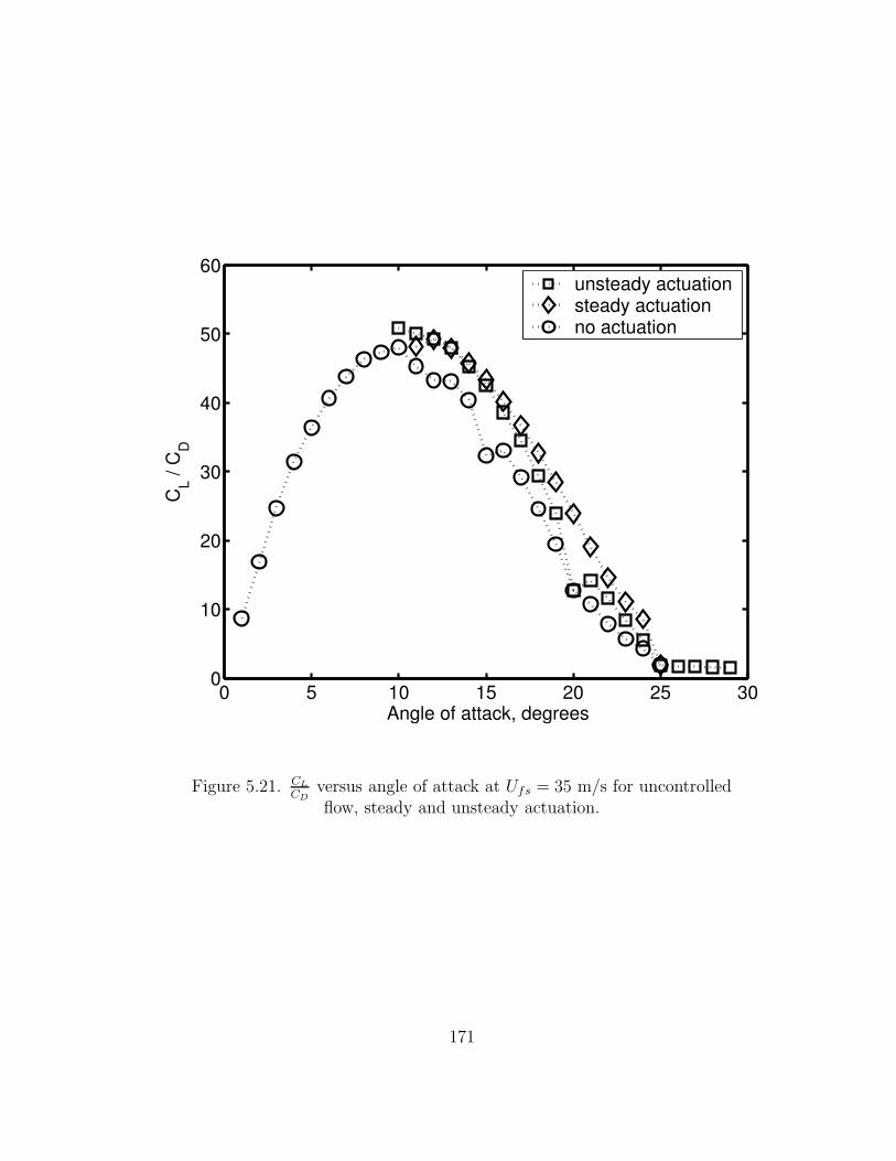
0 5 10 15 20 25 300
10
20
30
40
50
60
Angle of attack, degrees
C L / C D
unsteady actuationsteady actuationno actuation
Figure 5.21. CL
CDversus angle of attack at Ufs = 35 m/s for uncontrolledflow, steady and unsteady actuation.
171

0 5 10 15 20 25 30
0
0.2
0.4
0.6
0.8
1
1.2
1.4
1.6
Angle of attack, degrees
C L
simulation, unsteady actuationsimulation, steady actuationsimulation, no actuationexperiment, no actuationexperiment, unsteady actuation
Figure 5.22. Comparison between numerical and experimental data forlift coefficient versus angle of attack for uncontrolled case, steady and
unsteady actuation. Numerical simulations performed at Ufs = 35 m/s.Experiment performed at Ufs = 30 m/s, adopted from [52].
172

CHAPTER 6
CONCLUSIONS AND RECOMMENDATIONS FOR FUTURE WORK
This chapter presents conclusions related to the study of the physics of the sin-
gle dielectric barrier discharge and the numerical model created to simulate it. In
addition it summarizes the results of the numerical simulation of the leading-edge
separation control on an airfoil. Finally it makes recommendations for the future
work toward understanding the physics of the plasma actuator and modifying the
electric circuit model to include these physics.
6.1 Conclusions
This section presents conclusions on the experimental investigation, modeling
and numerical simulation of the plasma discharge and its application to leading-
edge separation control.
6.1.1 Physics of Discharge
The single dielectric barrier discharge plasma actuator was characterized through
a set of experiments. The focus was on the study of the light emission from the
plasma actuator related to the plasma formation on the dielectric surface. These
experiments were fundamental in understanding the physics of the discharge on
the time scale associated with the applied a.c. cycle.
173

The double-slit photomultiplier was used to measure the light emission from
the plasma actuator. Through the comparison with the electric current results,
it was shown that the light emission directly correlated with the formation of
the plasma discharge, and could be used as the measure of the volume of plasma
on the dielectric surface. The light emission was measured while varying several
parameters. One of the parameters was the applied a.c. voltage amplitude. The
other parameter varied was the applied a.c. frequency.
The photomultiplier experiments revealed a very complex structure of the
plasma discharge. During the operation of the plasma actuator, the plasma ap-
pears on the surface of the dielectric near the overlap junction of the electrodes.
The volume of the plasma increases during the a.c. cycle, and the plasma sweeps
across the surface. Given that the covered electrode is sufficiently wide, the plasma
growth stops when the voltage difference across the plasma region becomes less
than the voltage needed to maintain the plasma. This happens when the applied
voltage reaches its maximum or minimum values. At this moment the plasma on
the dielectric surface quenches.
The effect of the applied voltage amplitude on the discharge characteristics
was investigated. For this, the a.c. frequency was kept constant at 5 kHz, and
the amplitude of the applied voltage was varied in the range of 5-10 kVp−p. The
total light emission from the plasma actuator was found to be L ∝ V7/2app . This
agreed with the experimental results of Post [61] for the maximum plasma induced
velocity and results of Enloe et al. [20, 21] for the thrust produced by the plasma
actuator. In this set of experiments it was also found that the plasma propagation
velocity increased slightly with the applied voltage amplitude. The plasma sweep
velocity was found to be in the range of 70-110 m/s. It was also found that the
174

maximum extent of the plasma increased linearly with the voltage amplitude.
These results agreed with the previous observations by Enloe et al. [20, 21].
The effect of the applied a.c. frequency was also studied. For this, a fixed
applied voltage amplitude of 5 kVp−p was used. In these experiments, the a.c.
frequency was changed in the range of 5-11 kHz. It was found that the extent
of the plasma over the dielectric surface did depend on the a.c. frequency. This
resulted in a strong linear dependence of the plasma sweep velocity on the a.c.
frequency. The observed sweep velocities were in the range of 80-180 m/s.
6.1.2 Electrostatic Model
In the experiments, it has been observed that there exist three different time
scales associated with the plasma actuator. The first time scale, relates to the
formation of the microdischarges, which is on the order of 10−8 seconds. The
second time scale, defined by the a.c. frequency of the applied voltage, is on
the order of 10−4 seconds. The largest time scale in the operation of the plasma
actuator is associated with the neutral fluid response time which is of the order
of 10−2 seconds.
This difference in time scales allowed us to construct a quasi-steady electro-
static model for the plasma actuator and to derive the plasma body force from
first principles. This model included the idea of the Debye shielding in the plasma.
The electrostatic model was used to study the asymmetric electrode arrangement.
The distribution of the electric potential, electric field and the charge density were
calculated near the electrodes. From these, the plasma body force was calculated.
The importance of accounting for the volume of the plasma over the covered
electrode was also shown. This was done by applying the spatial weighting to the
175

body force results. The exponential form of the weighting function was chosen
to reflect the experimental observations. Another type of the weighting that was
used was a temporal weighting. It represented the linear growth of the volume of
plasma during the a.c. cycle.
The spatially weighted and temporally-spatially weighted plasma body forces
were used in the flow solver to model the flow in the closed box with the plasma
actuator located on the bottom wall. The plasma body force computed separately,
was introduced into the right hand side of the momentum equation point by point.
The numerical simulations showed the formation and growth of a starting
vortex that was previously observed in the experiments by Post [61]. It was also
shown that at T → ∞, the induced flow developed into a the jet flow with the fluid
drawn to the actuator and then accelerated downstream. The velocity profiles in
the similarity region were used to compare the solutions for the spatially weighted
and temporally-spatially weighted plasma body force cases. It was shown that the
flow development was similar in both cases, but the maximum velocities in the jet
were lower in case of the temporal-spatial weighting.
It was shown that the electrostatic model could be used to simulate the aero-
dynamic plasma actuator if the volume of plasma was know for the particular
applied voltage conditions. An attempt to extrapolate these results to other volt-
age amplitudes was not possible with this model.
6.1.3 Lumped-element Circuit Model
To account for the change in the volume of plasma with respect to the applied
voltage amplitude and frequency, the lumped-element circuit model was created.
This model represented the plasma actuator as a parallel network of resistive and
176

capacitive elements. The capacitive elements representing the dielectric allowed
us to model the accumulation of the charge on the surface of the dielectric.
Two types of the lumped-element circuit models were tested. The first model
was a coarse spatial lumped-element circuit model. In this model, the plasma was
represented by the time-varying resistive and capacitive elements. The values of
these depended on the volume of the plasma present over the dielectric. As tests
of this model showed, the power dissipated in the plasma actuator was P ∝ V7/2app .
This result is consistent with the results of Post [61] for the maximum velocity in
the plasma jet and Enloe et al. [20, 21] for the thrust produced by the plasma
actuator.
The second model was a spatial-temporal lumped-element circuit model. It was
developed to simulate the internal structure of the plasma discharge. This model
represented the plasma a series of parallel networks, each consisting of resistive
and capacitive elements, and zenor diodes that controlled the values based on the
current direction. The advantage of this model was that it could investigate the
effect of amplitude and frequency without the need of experimentally determined
coefficients. Prior to any other tests, this model was tested for the optimal number
of parallel sub-circuits.
The space-time lumped-element circuit model allowed us to obtain the in-
formation about the current in the plasma, which has been shown previously to
correlate directly to the light emission form the plasma. The results of the current
distribution were found to be consistent with the light intensity measurements.
The effect of the applied voltage amplitude and a.c. frequency on the plasma
characteristics was examined with the space-time lumped-element circuit model.
The results were found to be in good agreement with the experimental results. The
177

maximum extent of the plasma was increasing linearly with the applied voltage
amplitude, but was almost constant over the entire range of the a.c. frequencies
tested. The plasma sweep velocity was found to increase linearly with the applied
voltage amplitude and a.c. frequency.
The results of space-time lumped-element circuit model were used to calculate
the time-resolved plasma body force. It was found that the plasma body force has
four peaks during the a.c. cycle, and that the direction of the plasma body force
is the same all the time. Spectral analysis performed on the plasma body force
time series showed that the dominating frequency in the spectrum was two times
the a.c. frequency.
The effect of the dielectric properties of the material was studied with the
space-time lumped-element circuit model. The plasma body force calculations
were performed for three different materials with ε = 10, 100, and 1000. It was
shown that for each material tested there exists an optimal frequency at which
the plasma body force is maximum. It was found that the optimal frequency
decreased as the dielectric coefficient increased. The power dissipated in plasma
due to ohmic heating monotonically increased with frequency. Therefore, too high
a frequency is inefficient in terms of converting the input power into the body force.
6.1.4 Leading-edge Separation Control
With this approach, the leading-edge separation control on NACA 0021 us-
ing single-dielectric barrier discharge plasma actuator was studied numerically.
FLUENT software was used to solve two-dimensional unsteady Reynolds-averaged
Navier-Stokes equations with the v2 − f turbulence model.
178

The plasma actuator was modeled on the leading edge of the airfoil. The
plasma body force computations were carried out using FemLab. The body force
was then introduced into the flow solver using the user defined function.
The effect of the plasma actuator body force on the fluid was studied in still
air. The formation of the starting vortex was observed near the actuator. The
steady plasma actuator working for a long time form a jet near the airfoil surface.
The unsteady plasma actuator was observed to form a periodic series of vortexes
near the leading edge.
First, the flow around the airfoil was computed without any actuation for a
range of angles of attack at 35 m/s inflow velocity. The convergence of the solution
was based on the lift and drag coefficients. It was shown that at the lower angles of
attack the airfoil characteristics were consistent with the linear airfoil theory, that
is having the slope dCL
dα= 2π. The aerodynamic stall of the airfoil was observed
at 18 degrees.
The leading-edge separation control with the steady and unsteady flow actu-
ation was studied numerically. During the steady actuation, the plasma body
force was permanently present. For the unsteady actuation, the body force was
present only for 10% of the duty cycle. The frequency of the unsteady actuation
corresponded to F+ = fc/Ufs = 1.
In both cases, the separation bubble was observed to become smaller. The
point of the separation was seen to move from the leading edge downstream to
half-cord of the airfoil. This reduction of the separation bubble resulted in the
increase of the lift and decrease of the drag of the airfoil.
It was found that the steady actuation increased the lift coefficient and delayed
the stall by approximately 2 degrees of angle of attack. The unsteady actuation
179

was shown to produce even better results. The stall angle in that case was in-
creased by 5 degrees. These results are consistent with the experiments for the
same conditions.
6.2 Recommendations For Future Work
6.2.1 Physical Properties of Plasma Discharge
Recent experiments have shown the superiority of the Teflon dielectric over
the traditional Kapton and PCB materials. This appears in the greater velocity
of the plasma induced jet, and therefore, in the greater momentum transfered
to the fluid. This advantage is probably due to the larger thickness of the Teflon
dielectric layer which leads to a more uniform plasma discharge without filaments.
This phenomenon of transition from the uniform plasma to filamentary discharge
needs to be studied. This can be done by measuring the light emission from
the filamentary and uniform plasma discharges using a photomultiplier. These
experiments may also be accompanied by the acoustical measurements from the
plasma actuator.
The SDB discharge plasma can also be studied optically with the fast CCD
camera. The rate of data acquisition of this type of cameras (up to 105 images per
second) allows one to obtain images of single discharge streamers. This informa-
tion can help to further improve our knowledge about the physics of the discharge
and refine the phenomenological model for plasma actuators.
In the present research one form of the input voltage signal has been studied,
particularly the sinusoidal wave form. Additional data needs to be collected for
different form of the input voltage signal to calibrate and test the space-time
lumped-element circuit model. PMT measurements of the light emission from
180

the plasma actuator may be done for the “triangle”, “positive sawtooth” and
“negative sawtooth” wave forms. These tests should be performed for the range
of different applied voltage amplitudes and a.c. frequencies. This would give the
information about the conditions of the plasma formation and quenching as well
as the dependence of the plasma characteristics on the voltage form.
The other open question in the physics of the SDB discharges is how the
momentum is transfered to the neutral fluid. There exist several theories which
propose the PUSH-push, PUSH-pull and other mechanisms for the plasma actu-
ators, meaning that during the a.c. cycle the plasma actuator creates a strong
and a weak body forces which act either in the same direction, or in opposite
directions. This question may be resolved by the velocity measurements directly
in the plasma region. Aero-optical laser devices and methods developed at the
University of Notre Dame may be used for this. In these methods, the density fluc-
tuations are estimated from the deflections of the laser light which passes through
the fluid. For this experiment, the glass may be used as the dielectric material,
and the bottom surface of this insulator may be cover with the reflecting material,
which would act as a mirror for the laser light. The velocity fluctuations may be
calculated from the obtained density fluctuations. These experiments are intended
to show if the fluid is accelerated during both halves of the a.c. cycle.
6.2.2 Improvements to the Lumped-element Circuit Model
Some improvements may be made for the lumped-element circuit model and
plasma body force computations. As mentioned in the previous subsection, the
plasma discharge may transition from the uniform regime to the filamentary
regime. This formation of filaments may be accounted for in the model through
181

introduction of another resistive element with a possibly lower resistance value.
This resistive element should be included into the circuit along with the zenor
diode element which would govern the initiation of the filaments. The condition
of this initiation may be possibly formulated using the voltage threshold for this
transition from the uniform plasma. The value of the transition threshold voltage
may be obtained experimentally.
The other improvement that may be done to the space-time lumped-element
circuit model regards the breakdown of the dielectric layer. The condition for this
breakdown and eventual shortage of the actuator circuit can be estimated from
the dielectric strength of the material used for insulation.
In this work, the Lumped-element circuit model was tested for the sinusoidal
applied voltage. In practical applications, the forms of the input signal are also
used, such as the triangle wave, the “positive” and the “negative” sawtooth signals.
The Lumped-element Circuit Model should be also tested for these forms of the
input voltage. The results may be compared to the existing experimental results.
Another modification may be done in terms of the charge density estimation
which is later used in the body force computations. The Lumped-element Circuit
model gives us the information about the electric current that flows through the
plasma actuator in each of the sub-circuits. This current is directly related to the
number of the charges and their velocities. This means that if we can estimate the
velocities of the charges in the plasma, then we can compute the ionization rate
in each of the sub-circuits, and calculate the plasma body force directly without
solving the Poisson electrostatic equation. The velocity of the charges can be
estimated in several different ways. For example, this can be done assuming the
Maxwell’s distribution for the gas particles.
182
6.2.3 Applications
The success of the numerical simulation of the leading edge separation control
open the possibilities for numerical study of other applications of the plasma
actuators for flow control. For example, the active boundary layer control on
the pitching airfoils may be studied computationally. The experimental data for
this type of flow control was gathered previously by M. Post [61]. This study
can be extended to include the plasma actuator into flow control on the micro air
vehicles, UAVs, and flapping wings. In this simulations, the optimal configuration
and active control strategy can be obtained for each flow control. This would help
to optimize the performance of the plasma actuators in the experiments.
Another aspect of the flow actuation, which is of big importance, deals with
the role played by the plasma actuators in the laminar-to-turbulent transition and
transition delay and control. This study may be done by utilizing the eN method,
which had been shown to work fairly well for the situations in which the level of
the free stream turbulence intensity is relatively low (flows around airfoils with
turbulence intensity < 1%).
183

BIBLIOGRAPHY
1. IMSL Fortran Subroutines for Mathematical Applications, 1977.
2. COMSOL Multiphysics 3.2 User’s Guide, 2005.
3. FLUENT 6.2 Documentation, 2005.
4. Gambit 2.2.30 Documentation, 2005.
5. MatLab 7.2.0.283 Documentation, 2006.
6. Anderson, D. A., Tannehill, J. C., and Pletcher, R. H. Computa-
tional Fluid Mechanics and Heat Transfer. Hemisphere Publishing Corpora-tion, 1984.
7. Anderson, R., and Roy, S. Preliminary Experiments of Barrier DischargePlasma Actuators Using Dry and Humid Air. AIAA Paper 2006-369, 2006.
8. Asghar, A., Jumper, E. J., and Corke, T. C. On the Use of ReynoldsNumber as the Scaling Parameter for the Performance of Plasma Actuator ina Weakly Compressible Flow. AIAA Paper 2006-21, 2006.
9. Baird, C., Enloe, C., McLaughlin, T., and Baughn, J. Acoustictesting of the dielectric barrier discharge (DBD) plasma actuator. AIAAPaper 2005-0565, 2005.
10. Batchelor., G. An Introduction to Fluid Dynamics. 1967.
11. Corke, T. C. Design of Aircraft. Prentice Hall Publishers, New York, 2002.
12. Corke, T. C., He, C., and Patel, M. Plasma flaps and slats: an appli-cation of weakly-ionized plasma actuators. AIAA Paper 2004-2127, 2004.
13. Corke, T. C., Jumper, E. J., Post, M. L., Orlov, D., and McLaugh-
lin, T. E. Application of weakly-ionized plasmas as wing flow-control devices.AIAA Paper 2002-0350, 2002.
184

14. Corke, T. C., Mertz, B., and Patel, M. P. Plasma Flow ControlOptimized Airfoil. AIAA Paper 2006-1208, 2006.
15. Douville, T., Stephens, J., Corke, T., and Morris, S. Turbine BladeTip Leakage Flow Control by Partial Squealer Tip and Plasma Actuators.AIAA Paper 2006-20, 2006.
16. Durbin., P. Separated flow computations with the k- ε- v2 model. AIAA
Journal 33 (1995), 659–664.
17. Enloe, C. private communications, USAF Academy, CO, 2004.
18. Enloe, C., McLaughlin, T., Font, G., and Baughn, J. Parametriza-tion of Temporal Structure in the Single Dielectric Barrier AerodynamicPlasma Actuator. AIAA Paper 2005-0564, 2005.
19. Enloe, C., McLaughlin, T., VanDyken, R., and Fuscher, J. Plasmastructure in the aerodynamic plasma actuator. AIAA Paper 2004-0844, 2004.
20. Enloe, L., McLaughlin, T., VanDyken, Kachner, Jumper, E., and
Corke, T. Mechanisms and responses odf a single-dielectric barrier plasmaactuator: Plasma morphology. AIAA 42 (2004), 589–594.
21. Enloe, L., McLaughlin, T., VanDyken, Kachner, Jumper, E.,
Corke, T., Post, M., and Haddad, O. Mechanisms and responses odf asingle-dielectric barrier plasma actuator: Geometric effects. AIAA 42 (2004),585–604.
22. Font, G. Boundary Layer Control with Atmospheric Plasma Discharges.AIAA Paper 2004-3574, 2004.
23. Font, G., and Morgan, W. L. Plasma Discharges in Atmospheric Pres-sure Oxygen for Boundary Layer Separation Control. AIAA Paper 2005-4632,2005.
24. Forte, M., Jolibois, J., Moreau, E., Touchard, G., and Cazalens,
M. Optimization of a Dielectric Barrier Discharge Actuator by Stationary andNon-stationary Measurements of the Induced Flow Velocity - Application toAirflow Control. AIAA Paper 2006-2863, 2006.
25. Gaitonde, D. V., Visbal, M. R., and Roy, S. Contol of Flow Past aWing Section with Plasma-based Body Forces. AIAA Paper 2005-5302, 2005.
26. Gibalov, V., and Pietsch, G. The development of dielectric barrier dis-charges in gas gaps and on surfaces. J.Phys.D 33 (2000).
185

27. Golubovskii, Y., Maiorov, V., Behnke, J., and Behnke, J. Influenceof interaction between charged particles and dielectric surface over a homo-geneous barrier discharge in nitrogen. Journal of Physics D: Applied Physics
35 (2002).
28. Hall, K., Jumper, E. J., Corke, T. C., and McLaughlin, T. E.
Potential Flow Model of a Plasma Actuator as a Lift Enchancement Device.AIAA Paper 2005-0783, 2005.
29. Hall, K. D. Potential flow model for plasma actuation as a lift enchancementdevice. Master’s thesis, University of Notre Dame, 2004.
30. Hoffmann, K. A., and Chiang, S. T. Computational Fluid Dynamics
For Engineers. Engineering Education System, 1993.
31. Huang, J. Documentation and control of flow separation on a linear cascade
of Pak-B blades using plasma actuators. PhD thesis, University of NotreDame, 2005.
32. Huang, J., Corke, T., and Thomas, F. Separation control over lowpressure turbine blades. In Bulletin of the American Physical Society Division
of Fluid Dynamics (2002), vol. 47.
33. Huang, J., Corke, T., and Thomas, F. Separation control over lowpressure turbine blades. In Bulletin of the American Physical Society Division
of Fluid Dynamics (2003), vol. 48.
34. Huang, J., Corke, T. C., and Thomas, F. O. Plasma actuators forseparation control of low pressure turbine blades. AIAA Paper 2003-1027,2003.
35. Hultgren, L. S., and Ashpis, D. E. Demonstration of separation delaywith glow-discharge plasma actuators. AIAA Paper 2003-1025, 2003.
36. Hussain, F., and Jeong, J. On the identification of a vortex. Journal of
Fluid Mechanics 285 (1995), 69–94.
37. Kakuta, S., Kamata, T., Makabe, T., Kobayashi, S., Terai, K.,
and Tamagawa, T. Study of surface charges on dielectric electrodes in aradio-frequency glow discharge. J.Appl.Phys. 77 (1995).
38. Kozlov, K., Wagner, H.-E., Brandenburg, R., and Michel, P.
Spatio-temporally resolved spectroscopic diagnostics of the barrier dischargein air at atmosperic pressure. J.Phys.D:Appl.Phys. 34 (2001).
186

39. Landau, L. D., and Lifshitz, E. Electrodynamics of continuous media.Pergamon, 1984.
40. Likhanskii, A., Shneider, M., Macheret, S., and Miles, R. Modelingof Interaction Between Weakly Ionized Near-Surface Plasmas and Gas Flow.AIAA Paper 2006-1204, 2006.
41. List, J., Byerley, A. R., McLaughlin, T. E., and VanDyken, R. D.
Using a plasma actuator to control laminar separation on a linear cascadeturbine blade. AIAA Paper 2003-1026, 2003.
42. Madani, M., Bogaerts, A., Gijbels, R., and Vangeneugden, D.
Modelling of a Dielectric Barrier Glow Discharge at Atmospheric Pressurein Nitrogen. In International Conference on Phenomena in Ionized Gases
(2003).
43. Massines, F., Rabehi, A., Decomps, P., Ben Gadri, R., Segur, P.,
and Mayoux, C. Experimental and theoretical study of a glow dischargeat atmosperic pressure controlled by dielectric barrier. Journal of Applied
Physics 83 (1998).
44. Matlis, E. H. Controlled experiments on instabilities and transition to tur-
bulence on a sharp cone at Mach 3.5. PhD thesis, University of Notre Dame,2004.
45. Morris, S. C., Corke, T. C., VanNess, D., Stephens, J., and Dou-
ville, T. Tip Clearance Control Using Plasma Actuators. AIAA Paper2005-0782, 2005.
46. Nelson, C., Cain, A., Patel, M., and Corke, T. Simulation of PlasmaActuators Using the Wind-US Code. AIAA Paper 2006-634, 2006.
47. Orlov, D., and Corke, T. Numerical simulation of aerodynamic plasmaactuator effects. AIAA Paper 2005-1083, 2005.
48. Orlov, D., Corke, T., and Haddad, O. DNS modeling of plasma arrayflow actuators. In Bulletin of the American Physical Society Division of Fluid
Dynamics (2003), vol. 48.
49. Orlov, D., Corke, T., and Patel, M. Electric Circuit Model for Aero-dynamic Plasma Actuator. AIAA Paper 2005-1206, 2006.
50. Orlov, D., Corke, T., and Post, M. DNS modeling of plasma arrayflow actuators. In Bulletin of the American Physical Society Division of Fluid
Dynamics (2002), vol. 47.
187

51. Orlov, D., Erturk, E., Post, M., and Corke, T. DNS modeling ofplasma array flow actuators. In Bulletin of the American Physical Society
Division of Fluid Dynamics (2001), vol. 46.
52. Orlov, D. M., Apker, T., He, C., Othman, H., and Corke, T. C.
Modeling and experiment of Leading-edge Separation Control Using Single-dielectric Barrier Discharge Plasma Actuators. AIAA Paper, 2007.
53. Pai, S., Guo, X., and Zhou, T. Closed form analytic solution describingglow discharge plasma. Phys.Plasmas 3 (1996).
54. Patel, M. P., Sowle, Z. H., Corke, T. C., and He, C. AutonomousSensing and Control of Wing Stall Using a Smart Plasma Slat. AIAA Paper2006-1207, 2006.
55. Paulus, M., Stals, L., Rude, U., and Rauschenbach, B. Two-dimensional simulation of plasma-based ion implantation. Journal of Applied
Physics 85 (1999).
56. Poggie, J. DC Glow Discharges: A Computational Study for Flow ControlApplications. AIAA Paper 2005-5303, 2005.
57. Porter, C., Baughn, J., McLaughlin, T., Enloe, C., and Font, G.
Temporal Force Measurements on an Aerodynamic Plasma Actuator. AIAAPaper 2006-104, 2006.
58. Post, M., and Corke, T. Separation control using plasma actuators. InBulletin of the American Physical Society Division of Fluid Dynamics (2002),vol. 47.
59. Post, M., and Corke, T. Airfoil leading-edge separation control usingplasma actuators. In Bulletin of the American Physical Society Division of
Fluid Dynamics (2003), vol. 48.
60. Post, M. L. Phased plasma actuators for unsteady flow control. Master’sthesis, University of Notre Dame, 2001.
61. Post, M. L. Plasma actuators for separation control on stationary and
unstationary airfoils. PhD thesis, University of Notre Dame, 2004.
62. Post, M. L., and Corke, T. C. Separation control on high angle of attackairfoil using plasma actuator. AIAA Paper 2003-1024, 2003.
63. Post, M. L., and Corke, T. C. Separation control using plasma actuators- stationary and oscillatory airfoils. AIAA Paper 2004-0841, 2004.
188
64. Roth, J. Industrial plasma engineering. Institute of Physics Publishing,1995.
65. Roth, J., Sherman, D., and Wilkinson, S. Electrohydrodynamic flowcontrol with a glow-discharge surface plasma. AIAA Journal 38 (2000).
66. Roy, S., and Gaitonde, D. V. Radio frequency induced ionized colli-sional flow model for application at atmospheric pressures. Journal of Applied
Physics (2004).
67. Roy, S., and Gaitonde, D. V. Modeling Surface Discharge Effects ofAtmospheric RF on Gas Flow Control. AIAA Paper 2005-0160, 2005.
68. Roy, S., Pandey, B., Poggie, J., and Gaitonde, D. V. Modelinglow pressure collisional plasma sheath with space-charge effect. Physics of
Plasmas 10 (2003), 2578–2585.
69. Shyy, W., Jayaraman, B., and Andersson, A. Modeling of glowdischarge-induced fluid dynamics. Journal of applied physics 92 (2002).
70. Siemens, W. Poggendorffs Ann. Phys. Chem. 102 (1857).
71. Suzen, Y., and Huang, P. Simulation of Flow Separation Contro usingPlasma Actuators. AIAA Paper 2006-877, 2006.
72. Suzen, Y., Huang, P., Jacob, J., and Ashpis, D. Numerical Simulationsof Plasma Based Flow Control Applications. AIAA Paper 2005-4633, 2005.
73. Thomas, F. O., Kozlov, A., and Corke, T. C. Plasma Actuators forBluff Body Flow Control. AIAA Paper 2006-2845, 2006.
74. Van Ness, D. K., Corke, T. C., and Morris, S. C. Turbine TipClearance Flow Control using Plasma Actuators. AIAA Paper 2006-21, 2006.
75. Visbal, M. R., and Gaitonde, D. V. Control of Vortical Flows UsingSimulated Plasma Actuators. AIAA Paper 2006-505, 2006.
76. Voikov, V., Corke, T., and Haddad, O. Numerical simulation of flowcontrol over airfoils using plasma actuators. In Bulletin of the American Phys-
ical Society Division of Fluid Dynamics (2004), vol. 49.
77. Wilkinson, S. private communications, NASA Langley Research Center,VA, 2003.
78. Wilkinson, S. P. Investigation of an Oscillating Surface Plasma for Turbu-lent Drag Reduction. AIAA Paper 2003-1023, 2003.
189