Embed Size (px)
Citation preview
i
MODELLING AND SIMULATION OF MODULAR REFINERY FOR
PRODUCTION OF FUELS WITH LOW ENVIRONMENTAL POLLUTION
Prepared by
Mbinzi Kita Deddy Ngwanza
(#1569064)
MSc Eng (Wits)
A thesis submitted to the Faculty of Engineering and the Built Environment,
University of the Witwatersrand, Johannesburg, in fulfilment of the requirements
for the degree of Master of Science in Engineering
Supervisor: Dr DiakanuaNkazi
Johannesburg, May 2020
I
Declaration
I declare that this thesis is my own unaided work. It is being submitted for the Degree of
Masters of Science to the University of the Witwatersrand, Johannesburg. It has not been
submitted before for any degree or examination in any other University.
Mbinzi Kita Deddy Ngwanza
10th
day of May year 2020
II
Abstract
Production and upgrading of fuels and petrochemicals, used worldwide, are based on a
type of refinery (characteristics, capacity), market, consumption demands, and
development of engine technology. Although the composition of crude oil differs by
origin, the key operations (units) performed are same. Crude oil distillation, cracking and
reforming constitute the operations’ key in oil refineries to produce useful product. Each
process has attracted more researches since the discovery of method separating crude oil
cuts. The complexed operations that occur in the production of fuels’ and their impact on
environment are reflected, paving the way for many additional researches.
Industrial processes cover a wide range of operations that deal with solids, liquids and
gases as feeding process or product. This requires a contribution from Chemical
Engineering science to solve any problem occurs during the operations. Modelling and
simulation are tools that are combined or useful on their own to solve real-life
troubleshooting situations, and/or upgrade researches. These can bring great advantages
to the industrial process.
Due to the need of upgrading petroleum refining products, this research aimed to develop
models and simulate the main refining units. Design data based on the characteristics of
crude oil, operating parameters of the involved units, and other essential data were
calculated and collected, and then entered into the Aspen Plus simulation software to
generate the modular refinery model. The results of the full simulation were studied and
allowed to obtain the composition of different products and to determine conditions of
petroleum products. This study shows that it is definitely possible to predict impact of
sulphur on environment. Different information on the modular refinery in this study were
obtained and used for the simulation. Simulation was performed using data such as the
number of trays (24), a reflux of 0.61, total catalyst flowrate of 6.92 m3/h, 36.42 m
3/h and
44.01 m3/h respectively for the hydrotreater, the reformer and the cracker; and the
composition of distillate, the bottom and the feed rate for paraffins, naphtenes and
aromatics.

III
Dedications
To my family members
IV
Publications
Paper accepted for publication by International Journal of Research and Review:
Mbinzi K. Deddy Ngwanza, D. Nkazi, H. Ngwanza and H Mukaya, 2018. “Review of
Catalytic processes design and modelling: Fluid Catalytic Cracking unit and Catalytic
Reforming unit”. International Journal of Research and Review 2018 - reviewed and
accepted for publication.
V
Conference(s) and seminar(s)
Date Place Nature of
presentation
Event
28 September 2017 Richard Ward Building,
Wits University
Poster Engineering Research Day
31 August 2018 Richard Ward Building,
Wits University
Oral
presentation
Oil and Gas group
research meeting
VI
Acknowledgements
Prima facie, I am grateful to God for the good health and wellbeing that were necessary
to complete this study.
I would like to pay particular tribute to the following key persons who have worked
closely with me in various ways during this period. You have assisted me more then you
thought.
I place on record, my sincere thank you to Dr Diakanua Nkazi, for his supervision,
inspiring guidance and support throughout this Masters journey.
I express my gratitude to the National Research Foundation for the financial assistance
throughout my second year of research.
I am also grateful to staff of the School of Chemical and Metallurgical Engineering of
University of the Witwatersrand for providing me with all the necessary facilities and
technical support for this research project.
I thank Mr Bruce Mothibedi for assisting me on the use of Wits-CHMT computer lab
facilities for simulation.
I owe more thanks to family. Words cannot express how grateful I am to my mother,
Anne Mulenga, and father, Norbert Ngwanza, for all the sacrifices that you have made on
my behalf. I thank my uncle and aunty, respectively Charles and Lorraine Ngwanza for
his dedication for the success of my studies.
Also I would like to thank my brothers and sisters for their endless support. Thanks to
Tiemele Aka, Olayile Ejekwu and Swathi Burla for their inputs during brainstorming
time. Lastly, I would like to thank my fiancée Pamela Kabila for her endless love and
support.
VII
Table of content
Declaration ................................................................................................ I
Abstract..................................................................................................... II
Dedications ............................................................................................. III
Publications ............................................................................................ IV
Conference(s) and seminar(s) ................................................................. V
Acknowledgements ................................................................................ VI
Table of content ..................................................................................... VII
List of Figures ........................................................................................ XI
List of Tables ......................................................................................... XII
List of Symbols .................................................................................... XIII
List of Abbreviations ....................................................................... XVIII
CHAPTER 1 INTRODUCTION ............................................................. 1
1.1. Background and motivation ............................................................................. 1
1.2. Research aims ..................................................................................................... 4
1.3. Research keys questions .................................................................................... 4
1.4. Expected outcomes ............................................................................................. 5
1.5. Outline of the dissertation ................................................................................. 5
CHAPTER 2 LITERATURE REVIEW ................................................ 6
2.1. Crude oil ............................................................................................................. 6
2.1.1. Basics of crude oil ............................................................................................ 6
2.1.2. Crude oil properties .......................................................................................... 7
2.2. Modular refinery ................................................................................................ 9
2.3. Process description........................................................................................... 11
2.3.1. Crude oil Distillation Unit .............................................................................. 13
2.3.2. Fluid Catalytic Cracking Unit ........................................................................ 14
2.3.3. Catalytic Reforming Unit ............................................................................... 15
2.3.4. Hydro Treatment Unit .................................................................................... 16
2.4. Background in Modelling and simulation of each unit of refinery ................ 17
VIII
2.4.1. Crude oil Distillation Unit .............................................................................. 17
2.4.2. Catalytic reforming unit ................................................................................. 20
2.4.3. Fluid Catalytic Cracking Unit ........................................................................ 23
2.4.4. Hydro-treating unit (HTU) ............................................................................. 25
2.5. Environmental aspects of refinery production.............................................. 28
CHAPTER 3 METHODOLOGY FOR DESIGN AND SIMULATION
OF PROCESS UNITS ............................................................................ 33
3.0. Introduction ......................................................................................................... 33
3.1. Methodology ..................................................................................................... 33
3.2. Modular refinery design basis and Process description ............................... 34
a) Crude oil Distillation Unit ................................................................................. 34
b) Fluid Catalytic Cracking Unit ............................................................................ 44
c) Catalytic Reforming Unit ................................................................................... 46
d) Hydrotreatment Unit .......................................................................................... 47
3.3. Modelling .......................................................................................................... 47
3.3.1. Distillation ...................................................................................................... 47
3.3.2. Fluid Catalytic Cracking ................................................................................ 51
3.3.3. Catalytic Reforming Unit ............................................................................... 53
3.3.4. Hydrotreatment modelling ............................................................................. 53
3.4. Simulation of modular refinery ...................................................................... 54
3.4.1. Process simulation procedure ......................................................................... 54
3.4.2. Process simulation .......................................................................................... 55
3.5. Environmental study ....................................................................................... 55
CHAPTER 4 RESULTS AND DISCUSSION ..................................... 58
4.1. General considerations .................................................................................... 58
4.1.1. Material and Energy balance .......................................................................... 58
4.1.2. Thermodynamic design considerations .......................................................... 59
4.1.3. Specific Gravity and characterization factor (K) ........................................... 62
IX
4.1.4. Volume average boiling point and Energy balance (enthalpy) ...................... 63
4.2. Crude Oil Distillation Unit design .................................................................. 64
4.2.1. Column parameters ........................................................................................ 64
4.2.2. Side strippers .................................................................................................. 61
4.3. Reactors design................................................................................................. 62
4.3.1. Trickle Bed Reactor ....................................................................................... 62
4.3.2. Catalytic reforming reactors ........................................................................... 62
4.3.3. Catalytic cracking reactor............................................................................... 63
4.4. Modelling .......................................................................................................... 64
4.4.1. Modelling of distillation ................................................................................. 64
4.4.2. Modelling of fluid catalytic cracking unit ...................................................... 69
4.4.3. Modelling of catalytic reforming unit ............................................................ 70
4.4.4. Modelling of Hydrotreatment unit ................................................................. 72
4.5. Simulation and results ..................................................................................... 72
4.5.1. Simulation steps on Aspen ............................................................................. 72
4.5.2. Simulation flow diagram ................................................................................ 72
4.5.3. Results of sulphur variation............................................................................ 74
4.6. Discussion.......................................................................................................... 76
CHAPTER 5 CONCLUSION AND RECOMMENDATION
.................................................................................................................. 81
5.1. Conclusions ....................................................................................................... 81
5.2. Recommendations ............................................................................................ 82
REFERENCES ....................................................................................... 84
APPENDIX ............................................................................................ 101
Appendix A: Feedstock data ................................................................................... 101
A.1. Thermodynmic properties data of the feedstock ................................................ 101
A.2. Physical, Chemical and thermodynamic properties ........................................... 105
X
A.4. Feed Items .......................................................................................................... 110
Appendix B: Material Balance and heat balance.................................................. 111
B.1. Material balance ................................................................................................. 111
B.2. Energy Balance .................................................................................................. 113
Appendix C: Crude Oil Distillation Uni design .................................................... 125
C.1. Column ............................................................................................................... 125
C.2. Side strippers ...................................................................................................... 127
Appendix D: Design of reactors .............................................................................. 128
D.1. Design of Hydrotreatment Unit reactor ............................................................. 128
D.2. Design of catalytic reforming reactors ............................................................... 129
XI
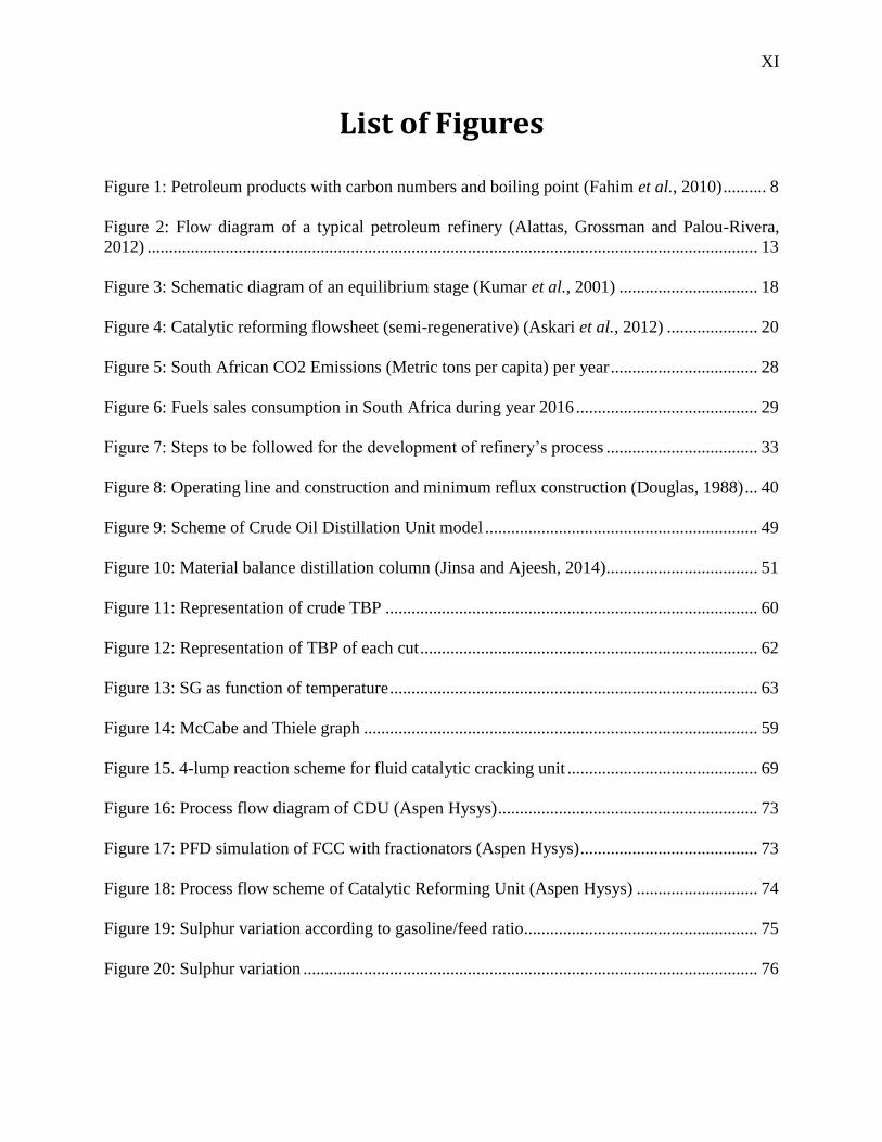
List of Figures
Figure 1: Petroleum products with carbon numbers and boiling point (Fahim et al., 2010) .......... 8
Figure 2: Flow diagram of a typical petroleum refinery (Alattas, Grossman and Palou-Rivera,
2012) ............................................................................................................................................. 13
Figure 3: Schematic diagram of an equilibrium stage (Kumar et al., 2001) ................................ 18
Figure 4: Catalytic reforming flowsheet (semi-regenerative) (Askari et al., 2012) ..................... 20
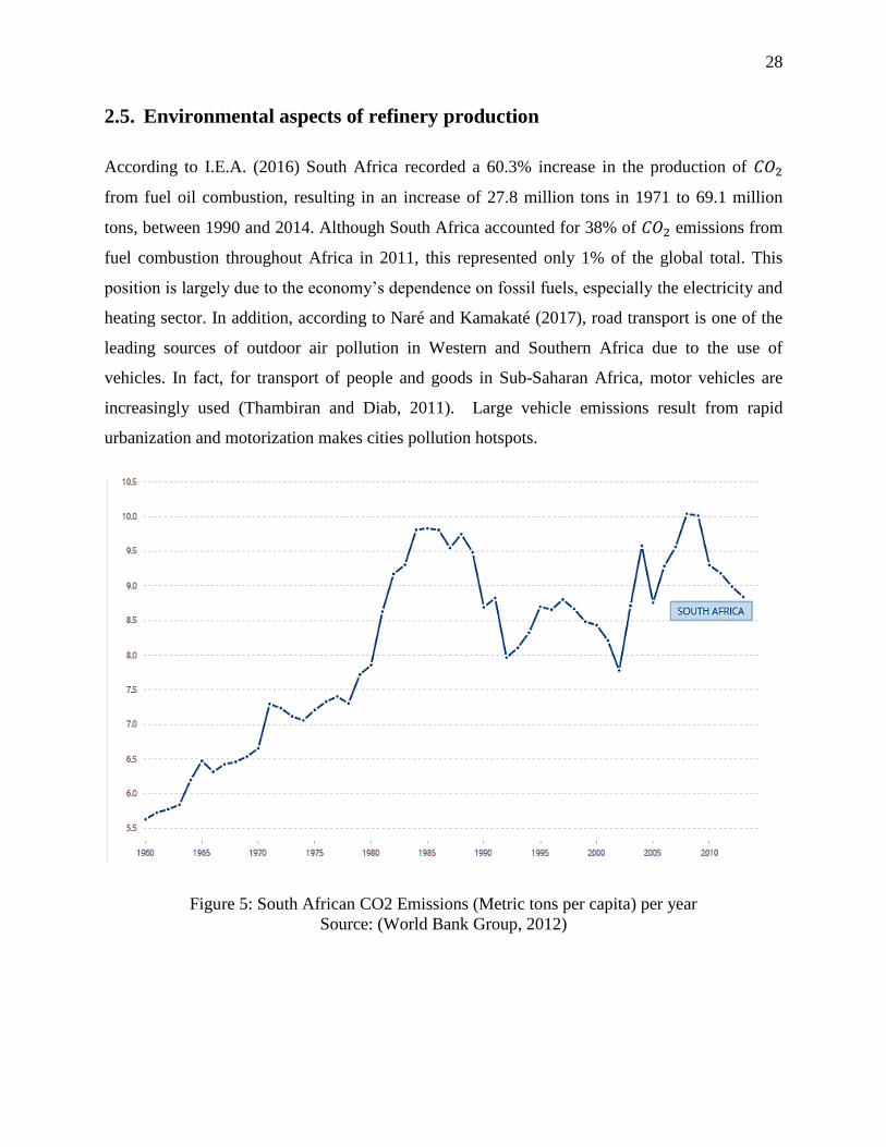
Figure 5: South African CO2 Emissions (Metric tons per capita) per year .................................. 28
Figure 6: Fuels sales consumption in South Africa during year 2016 .......................................... 29
Figure 7: Steps to be followed for the development of refinery’s process ................................... 33
Figure 8: Operating line and construction and minimum reflux construction (Douglas, 1988) ... 40
Figure 9: Scheme of Crude Oil Distillation Unit model ............................................................... 49
Figure 10: Material balance distillation column (Jinsa and Ajeesh, 2014)................................... 51
Figure 11: Representation of crude TBP ...................................................................................... 60
Figure 12: Representation of TBP of each cut .............................................................................. 62
Figure 13: SG as function of temperature ..................................................................................... 63
Figure 14: McCabe and Thiele graph ........................................................................................... 59
Figure 15. 4-lump reaction scheme for fluid catalytic cracking unit ............................................ 69
Figure 16: Process flow diagram of CDU (Aspen Hysys) ............................................................ 73
Figure 17: PFD simulation of FCC with fractionators (Aspen Hysys) ......................................... 73
Figure 18: Process flow scheme of Catalytic Reforming Unit (Aspen Hysys) ............................ 74
Figure 19: Sulphur variation according to gasoline/feed ratio ...................................................... 75
Figure 20: Sulphur variation ......................................................................................................... 76
XII
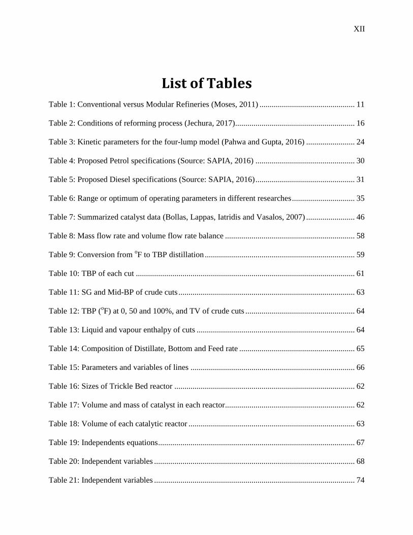
List of Tables
Table 1: Conventional versus Modular Refineries (Moses, 2011) ............................................... 11
Table 2: Conditions of reforming process (Jechura, 2017) ........................................................... 16
Table 3: Kinetic parameters for the four-lump model (Pahwa and Gupta, 2016) ........................ 24
Table 4: Proposed Petrol specifications (Source: SAPIA, 2016) ................................................. 30
Table 5: Proposed Diesel specifications (Source: SAPIA, 2016) ................................................. 31
Table 6: Range or optimum of operating parameters in different researches ............................... 35
Table 7: Summarized catalyst data (Bollas, Lappas, Iatridis and Vasalos, 2007) ........................ 46
Table 8: Mass flow rate and volume flow rate balance ................................................................ 58
Table 9: Conversion from oF to TBP distillation .......................................................................... 59
Table 10: TBP of each cut ............................................................................................................ 61
Table 11: SG and Mid-BP of crude cuts ....................................................................................... 63
Table 12: TBP (oF) at 0, 50 and 100%, and TV of crude cuts ...................................................... 64
Table 13: Liquid and vapour enthalpy of cuts .............................................................................. 64
Table 14: Composition of Distillate, Bottom and Feed rate ......................................................... 65
Table 15: Parameters and variables of lines ................................................................................. 66
Table 16: Sizes of Trickle Bed reactor ......................................................................................... 62
Table 17: Volume and mass of catalyst in each reactor ................................................................ 62
Table 18: Volume of each catalytic reactor .................................................................................. 63
Table 19: Independents equations ................................................................................................. 67
Table 20: Independent variables ................................................................................................... 68
Table 21: Independent variables ................................................................................................... 74
XIII
List of Symbols
accumulation of mass on the stage while
Wi is liquid holdup at stage i for
component j
𝑑(𝑊𝑖𝑥𝑖,𝑗)
𝑑𝜃
Active surface area of the stage and
surface area of the down corner
𝐴𝑇𝑖 and 𝐴𝐷𝑖
Actual composition of vapour entering
𝑛𝑡ℎtray
𝑌𝑛−1,𝑗𝑇
Actual number of tray 𝑁𝑎𝑐𝑡𝑢𝑎𝑙
Actual Reflux 𝑅𝑎𝑐𝑡𝑢𝑎𝑙:
Adsorption terms for the metal function
and for the acid function respectively
θ and Γ
Ammonia NH3
Antimony Sb
Area of heat transfer pertaining to the
convection
Aconv
Area of heat transfer pertaining to the
radiant
Arad
Average molecular weight 𝑀
Characterization factor 𝐾𝑊
Cold stream inlet temperature 𝑡1
Cold stream outlet temperature 𝑡2
Commercial cobalt-molybdenum on
alumina
Co-Mo/γ-Al2O3
Composition of component (i) in Feed 𝒛𝒊
Composition of light component in feed 𝑍𝐹
Constant mass transfer coefficient 𝑘𝐿
density difference between aqueous and ∆𝜌
XIV
organic phases, kg/m3
Catalyst to Oil Ratio COR
Density of liquid at stages i 𝜌𝐿𝑖
Density of the catalyst 𝜌𝐶𝑎𝑡
Density of the mixture 𝜌𝐺
Diameter of the tower 𝐷𝑇
Dioxide of carbon 𝐶𝑂2
Drop radius, m 𝑟
Efficiency 휀
Equilibrium coefficient for component j 𝐾𝑗
European emission standards Euro 1/2/3/4/5
Factor used to correct the departure from
true counter current flow
𝐹𝑇
Feed 𝑭
Feed quality 𝒒
Feed rate of input stream 𝐹
Flow rate of catalyst 𝑄𝑐𝑎𝑡
Flux of A into the liquid through the
liquid film as a function of driving force
𝑁𝐴
Fractional recovery of light in the bottom 𝛿
Fractional recovery of light in the
distillate
𝛽
From molecule with five carbon to
molecule with twelve carbon
C5-C12
From molecule with one carbon to
molecule with four carbon
C1-C4
Fugacity coefficient of the vapour phase Φ𝑖
Gravity, m/s2 𝑔
Heat transfer rate 𝑄
Heat transfer surface area[m2]
𝐴
XV
Height of column 𝐻𝑡𝑜𝑤𝑒𝑟
Hot stream inlet temperature 𝑇1
Hot stream outlet temperature 𝑇2
Hydrocarbon molecule R
Hydrogen sulphide H2S
Independent variables for the ith stage of
multicomponent distillation problem
𝑥𝑖,𝑗 ,𝐿𝑖, 𝑉𝑖and 𝑇𝑖
Iron Fe
Liquid enthalpy for jth component on ith
stage
ℎ𝑖,𝑗
Liquid flow from the process 𝐿𝑖
Liquid flow into the process 𝐿𝑖 𝑓𝑒𝑒𝑑
Liquid height of the stage ℎ𝑇𝑖
Log mean temperature difference ∆𝑇𝑀 ∆𝑇𝐿𝑀
Mean Average Boiling Point Mid-BP
Mean temperature difference ∆𝑇𝑀
Minimum reflux 𝑅𝑚𝑖𝑛
Molar density 𝜌𝑚
Molar enthalpies of inlet and outlet
streams
ℎ𝑖, ℎ𝑖+1, ℎ𝑖−1and ℎ𝐹𝑖
Mole flow of liquid from and entering
stage i
𝐿𝑖 and 𝐿𝑖−1
Mole flow of vapours from and entering
stage i
𝑉𝑖 and 𝑉𝑖+1
Mole fraction of jth component in liquid
phase on ith stage
𝑥𝑖,𝑗
Mole fraction of light component in
bottom
𝑋𝐵
Mole fraction of light component in
distillate
𝑋𝐷
XVI
Mole fractions in feed 𝑓
Mole fractions in liquid and vapour 𝑥 and 𝑦
Mole ratio of light component in feed 𝑍𝐹
Molecular weight of gas 𝑀𝐺
Molecular weight of the products 𝑀𝐵
Molecular weight of the reactants 𝑀𝐴
Murphree vapour efficiency for
𝑗 𝑡ℎcomponent on 𝑛𝑡ℎtray
Nitrogen Oxides NOx
Overall transfer coefficient 𝑈
Parts per million Ppm
Phase equilibrium constant of jth
component on ith stage
𝐾𝑖,𝑗
Polycyclic Aromatic Hydrocarbons PAH
Position of vapour in phase equilibrium
with liquid on nth tray with
composition 𝑋𝑛𝑗, 𝑌𝑛𝑗 actual composition
vapour leaving 𝑛𝑡ℎtray
𝑌𝑛𝑗∗
Rates constants of catalytic reforming
reactions
𝐾𝑒1,𝑘𝑓1,𝐾𝑒2,𝑘𝑓2, −𝑟𝑛𝑎𝑝ℎ𝑡ℎ𝑒𝑛𝑒−𝑐𝑟𝑎𝑐𝑘𝑖𝑛𝑔,
𝑘𝑓3, −𝑟𝑝𝑎𝑟𝑎𝑓𝑓𝑖𝑛−𝑐𝑟𝑎𝑐𝑘𝑖𝑛𝑔, 𝑘𝑓4
Rates equations of catalytic reforming
reactions
𝑟
Reflux ratio 𝑅
Relative volatility 𝛼
Residence time 𝑡𝐶
Respectively fugacity coefficient of pure
components in liquid phase and activity
coefficients and
𝜈𝑗0 and 𝛾𝑖
Respectively the heat of mixing, external
heat source and the heat losses
𝑄𝑀, 𝑄𝑆 and 𝑄𝑙𝑜𝑠𝑠
XVII
Settling rate V
Side stream 𝑆𝑖
Specific enthalpy of the feed ℎ𝑓
Specific enthalpy of the feed ℎ𝑖
Sulphur S
Sulphur Dioxide SO2
The heat flux in the radiant section 𝑞𝑟
The heat flux which occurs in the
convection section
𝑞𝑐
Theoretical number of tray 𝑁𝑡ℎ𝑒𝑜𝑟𝑦
Total bottom amount 𝐵
Total distillate amount 𝐷
Total distillate flow rate 𝐷
Total liquid flow rate from ith stage 𝐿𝑖
Total vapour flow rate of ith stage 𝑉𝑖
Valve sizing coefficient 𝐶𝑉
Vapour enthalpy for jth component 𝐻𝑖,𝑗
Vapour velocity 𝑉
Viscosity of oil, kg/m1s 𝜇0
Volume average boiling point 𝑇𝑉
Volume of reactor 𝑉𝑟𝑒𝑎𝑐𝑡𝑜𝑟
Volume of the catalyst 𝑉𝐶𝑎𝑡
Weight percent wt%
XVIII
List of Abbreviations
Abbreviation Meaning
ADU: Atmospheric Distillation Unit
AG: Atmospheric Gasoil
API gravity: American Petroleum Institute gravity
BP: Boiling Point
BPD: Barrels per day
CF2/3: Clean Fuels 2/3
CDU: Crude oil Distillation Unit
CRU: Catalytic Reforming Unit
D: Distillate
DEA-RSA: Department of Environmental Affairs, Republic of South Africa
EPA: United States Environmental Protection Agency
EU: European Union
FCCU: Fluid Catalytic Cracking Unit
FUG: Fenske-Underwood-Guilliland
HDAs: Hydrodeasphatenization
HDM: Hydrodemetallization
HDNi: Hydrodenickelation
HDS: Hydrodesulphurization
HDV: Hydrodevanadization
HK: Heavy Key
HN: Heavy Naphtha
HNK: Heavy Non-Key
HTU: HydroTreatment Unit
IEA: International Energy Agency
K: Kerosene
LK: Light Key
LN: Light Naphtha
XIX
LNK: Light Non-Key
LPG: Liquefied Petroleum Gas
MESH: Mass balance, Equilibrium, Summation and Heat relations
Mid-BP: Mean Average Boiling Point
PetroSA: Petrol, oil and gas corporation of South Africa
PIONA: Paraffin, Isoparaffin, Olefin, Naphtene and Aromatic
PM: Particle Matter
PNA: Paraffin, Naphtene and Aromatic
PONA: Paraffin, Olefin, Naphtene and Aromatic
R: Reflux
RON: Research Octan Number
RVP: Reid vapor pressure
SAPIA: South African Petroleum Industry Association
SARA: Saturated Aromatic, Resine and asphaltene
TBP: True Boiling Point
VDU: Vacuum Distillation Unit
VG: Vacuum Gasoil
VGO: Vacuum Gasoil
WSHV: Weight Hourly Space
1
CHAPTER 1
INTRODUCTION
1.1. Background and motivation
In this century, due to several lifestyles changes, the use and demand of petroleum products in
various fields (industry, transport, heating, electricity, …) has grown rapidly, making petroleum
the most important consumed substances in modern society (Khim, 2013; Ejikeme-Ugwu, 2012;
Speight, 2006). In fact, with 80% of global demand for transportation fuels met by petroleum
products, crude oil is the most widely used energy source in the world (Behmiri and Manso,
2014). However, crude oil is responsible for emissions of Carbon Dioxide (𝐶𝑂2), Sulphur
Dioxide (𝑆𝑂2), Nitrogen Oxides (𝑁𝑂𝑥) and Particulate Matter (PM). As a consequence, global
warming, stratospheric ozone depletion and climate change are due to these emissions. Harmful
emissions have therefore posed a pollution problem to the world that requires scientific research
to provide alternative and safe energy sources.
In many developing and transition countries, transport activities account for more than 50 % of
urban air pollution (PCFV, 2015). Developed countries have made significant investments in
cleaner and more efficient transport to reduce emissions (PCFV, 2015). Similar environmental
approaches have been adopted by encouraging the use of cleaner fuels and vehicle emissions
standards.
This research project focuses on modelling and simulation of a modular refinery to mitigate
negative emissions and provide cleaner fuels. A project of this nature is particularly necessary of
the aging of South Africa’s refining infrastructure, which has a negative impact on crude oil
production processes (Wakeford, 2012). Recognizing the ever-increasing demand for oil
products for both local and export consumptions, researchers consider that the environmental
benefits of cleaner fuels are essential for reducing the greenhouse gas emissions responsible for
global warming. Thus, a mathematical modelling process in this research provides a basis for a
process intervention to mitigate the unsustainable costs currently affecting South African
refineries.
2
Pollution and clean fuels issues have taken prominent place in international debates, and South
Africa is no exception. Desired levels of reduction of harmful emissions are critical in this
debate. Ranked 14th in 2018 by the International Energy Agency (IEA), South Africa is one of
the largest countries contributing to global greenhouse gas emissions and among the largest in
Africa (McSweeney and Timepley, 2018). From 27.8 million tonnes in 1971, South Africa has
increased its production of 𝐶𝑂2 from fuel combustion-oil by 60.30% in2014 (I.E.A., 2016). This
position is largely due to the economy’s dependence on fossil fuels.
According to the manufacturers companies, the main drivers of energy efficiency are new
environmental regulations coupled with costs of reducing emissions. Improving the energy
efficiency of companies means that their carbon footprints that allow to improve their position in
face of the challenges and costs resulting from 𝐶𝑂2 regulations (Bunse, Vodicka, Schönsleben,
Brülhart and Ernst, 2011). The influence of the quality of air emissions from various sources
should therefore begin to focus on the production of clean fuels at source. Various industries are
faced the need to produce environmentally friendly fuels, so that the scientific level researchers
must look for scientific leads to this end. This research is therefore aimed at proposing formulae
and processes that can leverage existing scientific and chemical provisions and enhance further
capabilities for refinement. An understanding of the composite constituents of existing fuels is
critical to provide a starting point for this research.
Refining is normally a combination of separation and purification processes that take into
account the required constituents of natural elements and organisms. Humans have been using
the separation process for a long time since the earliest civilizations. They developed the
extraction of metals from ores, flowers perfumes, plants dyes, and potash from ashes of burnt
plants, salt from sea water evaporation, refining of rock asphalt, and liquors distillation (Seader
et al., 2011). Separation processes and the use made of these extracts have always resulted in
determining the quality, the nature and the impact of the final product. An understanding of the
composition of petroleum will serve to further demonstrate the importance of these separation
processes.
Petroleum is an extremely complex product among hydrocarbon compounds and the use of its
various components depends on the separation process used. Several complex and intensive
3
processes are used to extract these components in order to formulate the final products. The
process of separation, conversion and treating is called crude oil refining process (Speight, 2006;
Yusuf, 2013). Crude oil processing comprises first, the separation process such as atmospheric
distillation and vacuum distillation; second, cracking and reforming processes to reduce heavier
hydrocarbons and increase hydrocarbon’s octane number; finally, a hydro-treatment process for
stabilizing and upgrading petroleum products (Jones and Pujadó, 2006; Yusuf, 2013). The
balance of use and formulae used in these processes determines the quality of the final product.
Certainly, fuel requirements are central to the operation of various industries. However, There is
a need to improve refining products and process in order to meet the environmental fuel
requirements, improve internal combustion and for economic reasons. The modelling and
simulation of chemical processes such as the crude distillation unit (CDU), the fluid catalytic the
cracking unit (FCCU), the cracking reformer unit (CRU), and hydro-treatment unit (HTU) can
alleviate problems by using software. In fact, HTU modelling helps meet environmental
requirements because it is the process that removes sulphur, nitrogen and aromatic; and
modelling of the CRU makes it to meet economic requirements as the aim of the process is to
upgrade the octane number in gasoline. The output of modelling could predict the process
behaviour and optimize the production process by improving operability and profitability
controls (Rao et al., 2004; Liu, 2015). A continuous search for enhancement and optimisation of
processes to produce more environmentally friendly fuels is therefore critical.
The aging of South Africa’s refining infrastructure affects the Crude oil processing operations,
and the processes review will help to improve the production of oil products. In fact, the last
significant changes fuels industry production in Southern Africa took place in 1980 when
PetroSA synthetic fuel facility was commissioned and Sasol shut down the synthetic fuel
production (Putter, 2015). Notably, the first South African crude oil refineries were built in
the1950s. It is becoming increasingly difficult to meet the modern standards of oil refining
industry sector. In South Africa, as well as in the rest of the world, demand for oil products has
increased as follows: Petrol by 35% and Diesel by 80% since 1990 (Putter, 2015). Production of
fuels with low environmental effect will be a solution of greenhouse effect and global warming.
Current South African refineries cost more to maintain and may become unsustainable in the
future.
4
1.2. Research aims
The aims of this project are to review the refining process for the production of petroleum
products with low environmental impact and simulate what enhances the production of
environment. To achieve these aims, this project will focus on the following objectives:
To Model and simulation of Crude oil Distillation Unit (CDU);
To investigate the Modelling and simulation of Catalytic Reforming Unit (CRU);
To investigate the Modelling and simulation of Catalytic Cracking unit (FCCU);
To investigate the Modelling and simulation of Hydrotreatment Unit (HTU).
There is compelling evidence world that it is more necessary than ever for the industry to use
cleaner fuels due to the rate of pollution that caused the emission of gasses that led to the
greenhouse effect. Chemical processes did not significantly reduce these emissions, which
required a more in depth study of the scientific and chemical processes used by the industry to
create viable options leading to creation of chemicals and fuels that have acceptable levels of
impact on the environment. The South African environment is not immune to the need for
cleaner fuels.
1.3. Research keys questions
This research seeks to answer the following main questions:
How can existing processes of modular refinery simulation and modelling be mathematically
manipulated to improve the refining of environmentally friendly fuels?
The sub questions emanating for the main research question are as follows:
1. Can existing processes of refinement be improved?
2. Can existing equations used in the refinement processes be updated to fit the environment
friendly requirement?
3. How can modelling and simulation of modular refinery achieve desired levels of fuel
purity?
5
1.4. Expected outcomes
Following outcomes resulted from this research effort:
Design of a modular refinery with distillation, catalytic cracking, catalytic reforming and
hydrotreatment as principal operations
Formulation of mathematical model for each unit considered.
Simulation of the modular refinery obtained after design
Environmental analyse of data obtained after simulation
1.5. Outline of the dissertation
The dissertation is structured as follows:
Chapter 1: This chapter provides a brief introduction to problems related to refining process and
implicit environmental aspects; briefly motivates the study and provides the aims of the research.
This chapter also outlines the steps followed to complete the project.
Chapter 2: This chapter summarize the theoretical underpinnings of the project, examining each
unit of the study and the environmental aspects of refinery production.
Chapter 3: This chapter discusses the Methodology used in this research and presents an
overview of elements of the refinery design and the presentation of modelling software used.
Chapter 4: This chapter presents the results obtained from the simulation of the designed model.
Chapter 5: This chapter provides a summary and the conclusion of the study. In addition, it
provides recommendations for future work.
6
CHAPTER 2
LITERATURE REVIEW
This chapter presents a review of the literature on finding cleaner energy through simulation and
modelling. Science and technology make extensive use of simulation and modelling to improve
various processes such as petroleum refining. In this chapter the review will include general
information on the origin and production of crude oil, an understanding of the constituent
products of crude oil, process description as well as the environmental consequences of refining.
An understanding of physical and chemical characteristics of crude oil, a modular refinery, a
description of refining process, a presentation of the overall design and environmental
regulations of refinery are required to build a model for crude oil separation plant. Each of these
topics is reviewed in this chapter.
2.1. Crude oil
Crude oil naturally exists in the form a mixture of hydro carbonates, organic compounds and
small amounts of metals. The nomenclatural culture around crude oil is based on their origins
and composition. The metamorphosis of organic matter in the earth’s crust is responsible for the
creation of crude oil, which is then refined to generate the petrochemicals used for various fuel
and energy needs. What follows is a detailed description of the constituencies of crude oil.
2.1.1. Basics of crude oil
As stated above, crude oil is a mixture of a myriad of hydrocarbons compounds from light
hydrocarbons such as methane, ethane, etc., to very heavy components. So called petroleum,
name taken from the Latin word meaning "rock oil"(Fagan, 1991). Throughout this study
reference to oil is synonymous to petroleum. The main constituents of petroleum are carbon and
hydrogen, besides that there are smaller amounts of non-hydrocarbon constituents such as
sulphur, nitrogen, oxygen and some trace elements (vanadium, nickel, iron and copper). In
general, crude oil contains on average 84% carbon, 14% hydrogen, 1%-3% sulphur, and less than
1% each of nitrogen, oxygen, metals, and salts (Cheremisinoff and Rosenfeld, 2009). Based on
7
the predominant proportion of similar hydrocarbon molecules crude oils are generally classified
as paraffinic, naphthenic, or aromatic. Mixed-base crudes contain varying amounts of each type
of hydrocarbon. Refinery crude base stocks usually consist of mixtures of two or more different
crude oils.
The composition of the numerous compounds of the crude oil depends on the geographical
location of exploitation. Although the chemical compositions are surprisingly uniform, their
physical characteristics vary considerably (Gary and Handwerk, 2001). Oil and natural gas were
formed hundreds of years ago from the prehistoric plants and animals. Deep organic matter in the
earth’s crust is converted to hydrocarbons over millions of years and is composed of oil and gas
(Speight, 2002; Tissot and Welte, 1984; Vanmali, 2014). This is caused by the thermal
maturation which occurs under extreme pressure and high temperature.
South Africa relies on imports feed for its refineries to attain the country’s liquid fuels needs
because of low levels of proven crude oil reserves and low crude oil production. Over 60% of
products refined locally are produced from imported crude oil from the following countries
(Ratshomo and Nembahe, 2015):
Saudi Arabia: about 50%
Nigeria: 24%
Ghana: 5%
Various producers: 7%
2.1.2. Crude oil properties
A complete analysis of crude oils is difficult because of their complex composition with different
hydrocarbon components creating complex mixtures. Fractionation and elemental analyses
applied to the fraction obtained are thus used to reach elemental analysis. Fractionation is a
separation process applied to mixtures to run a stepwise process of reducing transient mixtures to
the final product required. Although, according to Wauquier (1994), the heaviest crude oil
fractions such as asphaltenes cannot be isolated and completely characterised by modern
analytical methods. The high boiling point of components is significantly influenced by physical
8
properties such as API gravity, which quantifies asphaltenes and resins in terms of percentage
(Fahim, Al-Sahhaf and Elkilani, 2012).
Various researches and studies on analytical techniques have largely contributed to
characterization of petroleum in order to level the complexity of the qualitative and quantitative
determination of crude oil composition (El-Hadi, 2015; Liu, 2015). Understanding the
composition of crude oil provides a premise for this study extrapolate the implicit impact of
modelling and simulation when refinement optionsare sought.
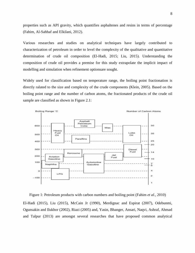
Widely used for classification based on temperature range, the boiling point fractionation is
directly ralated to the size and complexity of the crude components (Klein, 2005). Based on the
boiling point range and the number of carbon atoms, the fractionated products of the crude oil
sample are classified as shown in Figure 2.1:
Figure 1: Petroleum products with carbon numbers and boiling point (Fahim et al., 2010)
El-Hadi (2015), Liu (2015), McCain Jr (1990), Merdignac and Espirat (2007), Odebunmi,
Ogunsakin and Ilukhor (2002), Riazi (2005) and, Yasin, Bhanger, Ansari, Naqvi, Ashraf, Ahmad
and Talpur (2013) are amongst several researches that have proposed common analytical
9
methods and techniques used to identify the crude oils and petroleum products’ characteristics.
According to these researches, a conclusive characterization can be summarized by finding:
Physico-chemical proprieties: Specific gravity, API gravity, Sulphur content, Pour point,
Total acid content, water content, Kinematic viscosity and boiling point.
Compositional analysis: PONA, PNA, PIONA, SARA, elements analysis.
Crude oil with high viscosities and high API gravities contains a large amount of sulphur and
sulphur compounds (Eβer, Wassersceid and Jess, 2004). Refering to this category, crude oil may
also be classified as sweet crude if it contains less than 0.5% or as sour crude if it contains more
than 0.5% sulphur impurity (Wlazlowski, Hagströmer and Giulietti, 2001).
Notions of the proprieties of crude oil are from the basis of the characterization of the feed that
will be further used in this study.
2.2. Modular refinery
Due to economic considerations, expansion of distribution facilities, location, environmental
regulations, removal of price control, desired products and commodities and chemical
processing, petroleum refineries have increased significantly in size and particularity for each
refinery, as well as many refineries of very small size have shut down in the 20th century (Ibsen,
2006; Gary and Handwerk, 2001). According to Cross, Desrochers and Shimizu (2013) there are
probably no more than two identical refineries although some may share a number of common
features and processes because of specificity of refineries processing crude oil. The multiplicity
of refineries in their variegated processes of use results in efficiencies; although they are
sometimes detrimental to environment.
It is difficult to make general comparisons between refineries because of differences in
processing flow, type of crude oil fed and products slate chosen, such as a 500,000.00 Barrels
Per Day (BPD) refinery and 2,000.00 BPD refinery produce a different variety of products
(Ibsen, 2006).
10
A conventional refinery is a plant made up of different complex processing units that contribute
to production of various petroleum products. These units are costly to build and maintain
sustainably. This type of refinery has to use a large space and is often built near coasts for easy
transport and access to other countries (Moses, 2011).
According to Cenam (2014) and Moses (2011) a modular refinery consists of module-based
equipment built to be easily and quickly transported, configured and customized as needed,
anywhere in the world. In another a modular refinery is a conventional refinery built in a
fragmented way (Brown et al, 2003). Modular refineries are made up of discrete parts which are
assembled into modules in less time during their construction. Assembling off-site, the modules
are delivered to the refinery site where connection is made quickly and easily. Modular refineries
offer customized products and a variety of sizes with a capacity ranging from 500.00 to
30,000.00 BPD of crude oil inlet. These are considered as mini refineries easy to relocate that
efficiently produce primary fuels (for consumption) as well as raw materials (petrochemical
industries). In general, the averages quantities of products made from a barrel of crude oil are
(EIA, 2014):
Gasoline: 46%
Diesel fuel and heating oil: 26%
Jet Fuel: 9%
Liquefied Petroleum: 6%
Asphalt: 3%
Other products: 10%
11
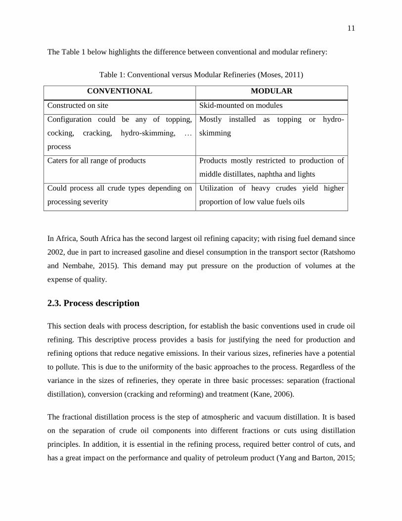
The Table 1 below highlights the difference between conventional and modular refinery:
Table 1: Conventional versus Modular Refineries (Moses, 2011)
CONVENTIONAL MODULAR
Constructed on site Skid-mounted on modules
Configuration could be any of topping,
cocking, cracking, hydro-skimming, …
process
Mostly installed as topping or hydro-
skimming
Caters for all range of products Products mostly restricted to production of
middle distillates, naphtha and lights
Could process all crude types depending on
processing severity
Utilization of heavy crudes yield higher
proportion of low value fuels oils
In Africa, South Africa has the second largest oil refining capacity; with rising fuel demand since
2002, due in part to increased gasoline and diesel consumption in the transport sector (Ratshomo
and Nembahe, 2015). This demand may put pressure on the production of volumes at the
expense of quality.
2.3. Process description
This section deals with process description, for establish the basic conventions used in crude oil
refining. This descriptive process provides a basis for justifying the need for production and
refining options that reduce negative emissions. In their various sizes, refineries have a potential
to pollute. This is due to the uniformity of the basic approaches to the process. Regardless of the
variance in the sizes of refineries, they operate in three basic processes: separation (fractional
distillation), conversion (cracking and reforming) and treatment (Kane, 2006).
The fractional distillation process is the step of atmospheric and vacuum distillation. It is based
on the separation of crude oil components into different fractions or cuts using distillation
principles. In addition, it is essential in the refining process, required better control of cuts, and
has a great impact on the performance and quality of petroleum product (Yang and Barton, 2015;
12
López et al., 2009). The objective here is to obtain C1-C4, naphtha/gasoline, kerosene, diesel and
atmospheric gasoil (Parkash, 2010).
With the aim of generating new hydrocarbons adapted to the desired products, the conversion
step can either break or combine molecules. From heavy hydrocarbons to smaller molecules, the
cracking process can be achieved by the thermal cracking or/and fluid catalytic cracking (FCC),
then converting heavy hydrocarbons (gas oils, residues) into lighter petroleum fractions
(gasolines, LPG) (Han et al., 2004; Barbosa et al., 2013). By often using naphtha as feed
catalytic reforming gives high yields of aromatics compounds such as benzene, toluene and
xylenes (Taskar, 1996). A combination process, such as alkylation and polymerization, links the
molecules together to form a larger molecule. From the light olefins available, larger amounts of
paraffinic high octane products can be made through alkylation although polymerization
produces highly photo-reactive olefins that contribute to visual pollution of the air and to the
production of ozone (Gary, Handwerk and Kaiser, 2007). The culmination of the cracking stage
is to prepare the resulting products for the next treatment.
The treatment step, also called purification process, has the role of eliminating impurities such as
sulphur compounds, nitrogen, metals and other impurities that can poison the catalysts and
responsible for pollution that is an environmental constraint (Fahim et al., 2010; Ferreira et al.,
2010). Any formula-based intervention should also target this stage of the process because it is
similar to the quality of the products obtained prior the blending stage.
The last phase in the process involves blending and this is the stage at which the product is
finalized for consumption. It is at this stage that the composition of the products indicates the
subsequent environmental impact. This stage must thus be achieved when everything is done to
minimize impurities in the final products placed on the market.
13
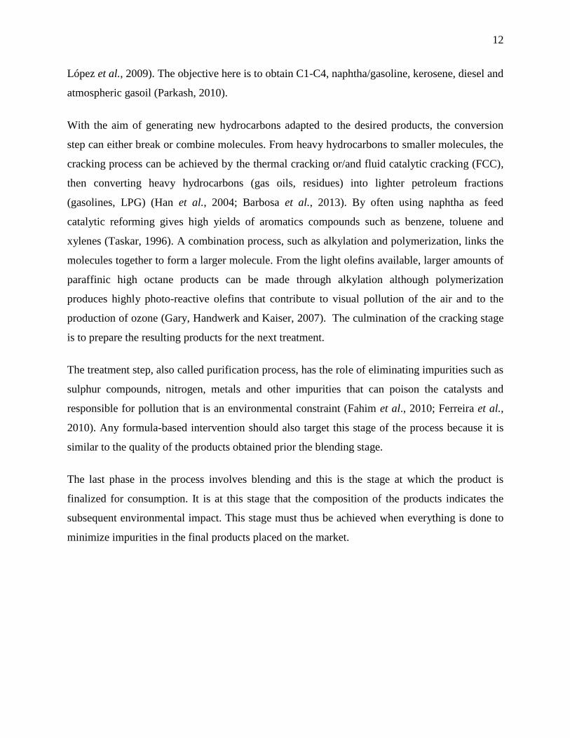
This research will focus on the some of the main units shown in the flow process below (Figure
2) which include: Crude oil Distillation Unit (CDU), Catalytic Reforming (Cat Ref), Catalytic
Cracking (Cat Crack), Hydrotreatment, and Blending Unit.
Figure 2: Flow diagram of a typical petroleum refinery (Alattas, Grossman and Palou-Rivera,
2012)
2.3.1. Crude oil Distillation Unit
Firstly, crude oil is fractionated in the atmospheric column (ADU) in order to obtain following
components: Off gas (LPG), naphtha, kerosene, atmospheric gasoil, diesel and the atmospheric
residue. Then the last component, namely atmospheric residue, undergoes fractionation in order
to obtain light, heavy gasoil and vacuum residue from long carbon chained molecules with very
high boiling points. This study covers both atmospheric columns products and vacuum columns
products.
Due to the composition of crude oil, it is important to follow some steps before starting the main
step of separation. In order to prevent corrosion and downstream poisoning, it is necessary to
eliminate the amounts of water and traces of inorganic accompanying oil, using a specific
process named desalting and dehydration separation systems (Ilkhaani, 2009). The Oil needs to
be heated using heat generating equipment (heater and preheater), which are furnaces or direct
combustion; in order to heat all types of hydrocarbons (Fuente, 2015). In addition to the furnace,
some devices are also used to transfer heat between a solid object and fluid, or between two or
14
more fluids, and this is called heat exchanger. Therefore, our research will consider desalting and
heating as pre-treatment step of crude oil.
The most important unit of the refining process is the atmospheric distillation unit (ADU). The
efficiency of this unit determines the processing at the subsequent steps of refining. The heated
crude oil (350oC-400
oC) is fed into the bottom of the column from where different components
come out as separate streams. The upper distillates will be gas and naphtha, the middle distillates
will contain kerosene, heavy and light gasoil, the lower distillates will be sent to the reboiler in
order to increase the degree of fractionation and overall efficiency and finally the atmospheric
residue will be injected to a furnace as required by the vacuum distillation unit (VDU). The VDU
operates in a range of 370 to 425oC temperature and pressure range of 350 to 1400.00 kg/m
2
(EPA, 1995). Products from the VDU are light vacuum gas oil, heavy vacuum gas oil and
vacuum residue (used to make asphalt). These details will be taken into account in the
configuration process.
2.3.2. Fluid Catalytic Cracking Unit
According to Sadeghbeigi (2000), the cracking unit is the key of the conversion process used in
refinery. The thermal cracking was the primitive way used to crack crude oil, but because of the
production of higher octane number gasoline, it was replaced by catalytic cracking (Hug, 1998).
During fluid catalytic cracking of petroleum, heavy hydrocarbons are converted to valuable
petroleum gasoline, olefin compounds (ethylene, propylene) having a carbon chain of more than
100 through fluidized catalytic cracking process (Han et al., 2000; Barbosa et al., 2013).
Notably, heavy hydrocarbons are high-molecular weight hydrocarbons fractions with a high-
boiling point. This study focuses on heavy gas oil such as atmospheric gas oil (AG) and vacuum
gas oil (VG) which constitute the feedstock of FCCU.
The foregoing products are both converted using catalysts made by combination of materials to
display a plurality of functions that behave as a liquid when fluidized (Sadeghbeigi, 2012). The
catalysts are a combination of acidic functions in amorphous and crystalline matrices, metal
impurity traps, combustion enhancers, sulphur oxide traps, octane boosters and olefins promoter
additives (Sadeghbeigi, 2012). What happens during catalytic cracking in a fluid medium is that
the feed is brought into contact with the catalyst at a temperature of about 500oC and at
15
moderately low pressures. Catalysts have four major components: zeolite, matrix, binder, and
filler (Doronin et al., 2007). The zeolites are chosen as particularly useful catalysts for gasoline
because zeolites give high percentages of hydrocarbons with between 5 and 10 carbon atoms.
Zeolite will therefore be the catalyst used in this study.
The main objective of the petroleum refinery is the production of fuels, which cannot be
achieved without valorization of fractionation products (Ancheyta, 2011). Fluid catalytic
cracking is one of the processes for upgrading production by conversion using catalysts. In
particular, the catalytic reforming is also a conversion process which uses catalysts whose
components have great similarities with the components present in the FCCU catalysts.
Therefore, the next section will deal with the process where chemical conversions take place to
the production of usable petrochemicals, thus addressing with the CRU.
2.3.3. Catalytic Reforming Unit
The CRU is a very important aspect of the process in terms of converting low-octane naphtha to
high-octane naphtha without any changing the number of carbons in the molecule, as well as the
producing a high yield of aromatics (benzene, toluene, and xylenes) in petroleum-refining and
petrochemical industries (Liang et al., 2005; Taskar, 1996). Hydrogen and lighter hydrocarbons
are also obtained as by-products. This must be taken into account in order to optimize the
amount of gasoline produce by the modular refinery.
The reforming feedstock is a complex mixture of normal and branched paraffins, five- and six-
membered ring naphthenes, and single-ring aromatics, having carbon number ranging from 6 to
11. A good reforming feed must have high naphtene and aromatic hydrocarbon content.
However, heavy fractions have good reforming, they have a strong tendency of coke formation
and lighter fractions have poor reforming capacity. The process built into our research must take
into account this important parameter.
During the catalytic process a number of conversion reactions occur, such as dehydrogenation of
naphthenes to aromatics and paraffins to olefins, dehydrocyclization of paraffins and olefins to
aromatics, isomerization of normal paraffins to isoparaffins, hydrocracking of paraffins and
naphthenes to lower hydrocarbons. The success of those different reactions helps to transform
16
low octane number to high octane number and aromatics into rich benzene. To achieve our
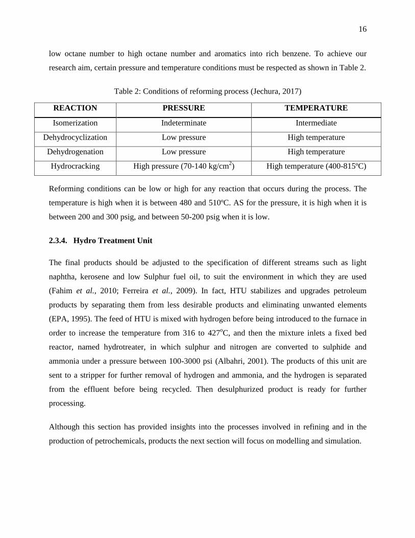
research aim, certain pressure and temperature conditions must be respected as shown in Table 2.
Table 2: Conditions of reforming process (Jechura, 2017)
REACTION PRESSURE TEMPERATURE
Isomerization Indeterminate Intermediate
Dehydrocyclization Low pressure High temperature
Dehydrogenation Low pressure High temperature
Hydrocracking High pressure (70-140 kg/cm2) High temperature (400-815ºC)
Reforming conditions can be low or high for any reaction that occurs during the process. The
temperature is high when it is between 480 and 510ºC. AS for the pressure, it is high when it is
between 200 and 300 psig, and between 50-200 psig when it is low.
2.3.4. Hydro Treatment Unit
The final products should be adjusted to the specification of different streams such as light
naphtha, kerosene and low Sulphur fuel oil, to suit the environment in which they are used
(Fahim et al., 2010; Ferreira et al., 2009). In fact, HTU stabilizes and upgrades petroleum
products by separating them from less desirable products and eliminating unwanted elements
(EPA, 1995). The feed of HTU is mixed with hydrogen before being introduced to the furnace in
order to increase the temperature from 316 to 427oC, and then the mixture inlets a fixed bed
reactor, named hydrotreater, in which sulphur and nitrogen are converted to sulphide and
ammonia under a pressure between 100-3000 psi (Albahri, 2001). The products of this unit are
sent to a stripper for further removal of hydrogen and ammonia, and the hydrogen is separated
from the effluent before being recycled. Then desulphurized product is ready for further
processing.
Although this section has provided insights into the processes involved in refining and in the
production of petrochemicals, products the next section will focus on modelling and simulation.
17
2.4. Background in Modelling and simulation of each unit of refinery
Simulation can be defined as usage of mathematical model to generate a certain description of
process behaviors. The main advantage of the simulation is to give a real view of the process
behavior (Rahim and Ben-Rahla, 2012).
Aspen Hysys was developed by AspenTech, a leading supplier of software that optimizes
process manufacturing for the energy, chemicals, pharmaceuticals, engineering and
constructions, and other industries that manufacture and produce products from chemical
processes (AspenTech, 2009).
This section serves to highlight further investigation of the different refinery units for which the
models used were based on the process illustrated in the Figure 2.
2.4.1. Crude oil Distillation Unit
In the pursuit of improving and developing rigorous models several researches and various
approaches have been advanced, especially in computer science. Such research has improved and
developed many tools, such as Aspen Plus (Aspentech), PRO/II (SimSci-Esscor), PROMS and
design IITM (ChemShare), which have been a feature of simulation and modelling (Li, Hui and
Li, 2005).
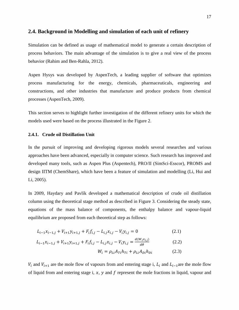
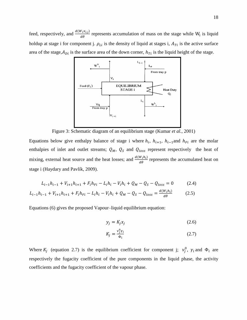
In 2009, Haydary and Pavlík developed a mathematical description of crude oil distillation
column using the theoretical stage method as described in Figure 3. Considering the steady state,
equations of the mass balance of components, the enthalpy balance and vapour-liquid
equilibrium are proposed from each theoretical step as follows:
𝐿𝑖−1𝑥𝑖−1,𝑗 + 𝑉𝑖+1𝑦𝑖+1,𝑗 + 𝐹𝑖𝑓𝑖,𝑗 − 𝐿𝑖,𝑗𝑥𝑖,𝑗 − 𝑉𝑖𝑦𝑖,𝑗 = 0 (2.1)
𝐿𝑖−1𝑥𝑖−1,𝑗 + 𝑉𝑖+1𝑦𝑖+1,𝑗 + 𝐹𝑖𝑓𝑖,𝑗 − 𝐿𝑖,𝑗𝑥𝑖,𝑗 − 𝑉𝑖𝑦𝑖,𝑗 =𝑑(𝑊𝑖𝑥𝑖,𝑗)
𝑑𝜃 (2.2)
𝑊𝑖 = 𝜌𝐿𝑖𝐴𝑇𝑖ℎ𝑇𝑖 + 𝜌𝐿𝑖𝐴𝐷𝑖ℎ𝐷𝑖 (2.3)
𝑉𝑖 and 𝑉𝑖+1 are the mole flow of vapours from and entering stage i, 𝐿𝑖 and 𝐿𝑖−1are the mole flow
of liquid from and entering stage i, 𝑥, 𝑦 and 𝑓 represent the mole fractions in liquid, vapour and
18
feed, respectively, and 𝑑(𝑊𝑖𝑥𝑖,𝑗)
𝑑𝜃 represents accumulation of mass on the stage while Wi is liquid
holdup at stage i for component j. 𝜌𝐿𝑖 is the density of liquid at stages i, 𝐴𝑇𝑖 is the active surface
area of the stage,𝐴𝐷𝑖 is the surface area of the down corner, ℎ𝑇𝑖 is the liquid height of the stage.
Figure 3: Schematic diagram of an equilibrium stage (Kumar et al., 2001)
Equations below give enthalpy balance of stage i where ℎ𝑖, ℎ𝑖+1, ℎ𝑖−1and ℎ𝐹𝑖 are the molar
enthalpies of inlet and outlet streams; 𝑄𝑀, 𝑄𝑆 and 𝑄𝑙𝑜𝑠𝑠 represent respectively the heat of
mixing, external heat source and the heat losses; and 𝑑(𝑊𝑖ℎ𝑖)
𝑑𝜃 represents the accumulated heat on
stage i (Haydary and Pavlík, 2009).
𝐿𝑖−1ℎ𝑖−1 + 𝑉𝑖+1ℎ𝑖+1 + 𝐹𝑖ℎ𝐹𝑖 − 𝐿𝑖ℎ𝑖 − 𝑉𝑖ℎ𝑖 + 𝑄𝑀 − 𝑄𝑆 − 𝑄𝑙𝑜𝑠𝑠 = 0 (2.4)
𝐿𝑖−1ℎ𝑖−1 + 𝑉𝑖+1ℎ𝑖+1 + 𝐹𝑖ℎ𝐹𝑖 − 𝐿𝑖ℎ𝑖 − 𝑉𝑖ℎ𝑖 + 𝑄𝑀 − 𝑄𝑆 − 𝑄𝑙𝑜𝑠𝑠 =𝑑(𝑊𝑖ℎ𝑖)
𝑑𝜃 (2.5)
Equations (6) gives the proposed Vapour–liquid equilibrium equation:
𝑦𝑗 = 𝐾𝑗𝑥𝑗 (2.6)
𝐾𝑗 =𝜈𝑗
0𝛾𝑖
Φ𝑖 (2.7)
Where 𝐾𝑗 (equation 2.7) is the equilibrium coefficient for component j; 𝜈𝑗0, 𝛾𝑖 and Φ𝑖 are
respectively the fugacity coefficient of the pure components in the liquid phase, the activity
coefficients and the fugacity coefficient of the vapour phase.
19
Known as MESH, mass balance, equilibrium, summation and heat relations are used to develop a
multicomponent distillation model suited for crude oil fraction at each stage, taking into account
variables such as total liquid and total vapour flow rates, mole fractions of the components, and
temperature (Haydary and Pavlík, 2009, Kumar et al., 2001).
In some cases, the nonlinear equations of systems have been solved using the Newton–Raphson
method by a correct choice of independent variables. This choice of variables makes the
proposed model numerically stable and robust, and has helped the authors to demonstrate the
stability and efficiency of the technique. The formulation founded by Kumar, Sharma,
Chowdhury, Ganguly and Saraf (2001) uses 𝑥𝑖,𝑗 ,𝐿𝑖, 𝑉𝑖 and 𝑇𝑖 as independent variables for the ith
stage of multicomponent distillation problem, and the mass balance, energy balances and
summation equations are given below:
𝐷𝐶𝑖,𝑗 = 𝑉𝑖+1𝐾𝑖+1,𝑗𝑥𝑖+1,𝑗 + 𝐿𝑖−1𝑥𝑖−1,𝑗 − 𝐿𝑖𝑥𝑖,𝑗 − 𝑉𝑖𝐾𝑖,𝑗𝑥𝑖,𝑗 (2.8)
𝐷𝐻𝑖 = 𝑉𝑖+1 ∑ 𝐾𝑖+1,𝑗𝑥𝑖+1,𝑗𝐻𝑖+1,𝑗 + 𝐿𝑖−1 ∑ 𝑥𝑖−1,𝑗ℎ𝑖−1,𝑗 − 𝐿𝑖 ∑ 𝑥𝑖,𝑗ℎ𝑖,𝑗 − 𝑉𝑖 ∑ 𝐾𝑖,𝑗𝑥𝑖,𝑗𝐻𝑖,𝑗 (2.9)
𝐷𝑉𝑖 = 𝑉𝑖 − 𝑉𝑖 ∑ 𝐾𝑖,𝑗𝑥𝑖,𝑗 (2.10)
𝐷𝐿𝑖 = 𝐿𝑖 − 𝐿𝑖 ∑ 𝑥𝑖,𝑗 (2.11)
With 𝐷: Total distillate flow rate
𝐻𝑖,𝑗: Vapour enthalpy for jth component
ℎ𝑖,𝑗: Liquid enthalpy for jth component on ith stage
𝐾𝑖,𝑗: Phase equilibrium constant of jth component on ith stage
𝐿𝑖: Total liquid flow rate from ith stage
𝑉𝑖: Total vapour flow rate of ith stage
𝑥𝑖,𝑗: Mole fraction of jth component in liquid phase on ith stage
20
2.4.2. Catalytic reforming unit
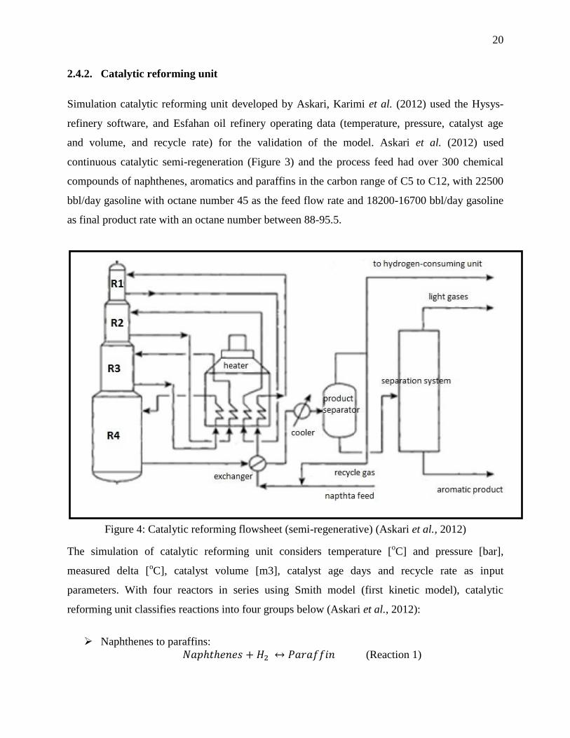
Simulation catalytic reforming unit developed by Askari, Karimi et al. (2012) used the Hysys-
refinery software, and Esfahan oil refinery operating data (temperature, pressure, catalyst age
and volume, and recycle rate) for the validation of the model. Askari et al. (2012) used
continuous catalytic semi-regeneration (Figure 3) and the process feed had over 300 chemical
compounds of naphthenes, aromatics and paraffins in the carbon range of C5 to C12, with 22500
bbl/day gasoline with octane number 45 as the feed flow rate and 18200-16700 bbl/day gasoline
as final product rate with an octane number between 88-95.5.
Figure 4: Catalytic reforming flowsheet (semi-regenerative) (Askari et al., 2012)
The simulation of catalytic reforming unit considers temperature [oC] and pressure [bar],
measured delta [oC], catalyst volume [m3], catalyst age days and recycle rate as input
parameters. With four reactors in series using Smith model (first kinetic model), catalytic
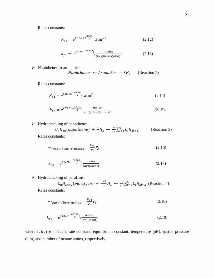
reforming unit classifies reactions into four groups below (Askari et al., 2012):
Naphthenes to paraffins:
𝑁𝑎𝑝ℎ𝑡ℎ𝑒𝑛𝑒𝑠 + 𝐻2 ↔ 𝑃𝑎𝑟𝑎𝑓𝑓𝑖𝑛 (Reaction 1)
21
Rates constants:
𝐾𝑒1 = 𝑒(−7.12+8000
𝑇), atm−1 (2.12)
𝑘𝑓1 = 𝑒(35.98−59600
𝑇),
𝑚𝑜𝑙𝑒𝑠
(ℎ𝑟)(𝑙𝑏𝑐𝑎𝑡)(𝑎𝑡𝑚)2 (2.13)
Naphthenes to aromatics:
𝑁𝑎𝑝ℎ𝑡ℎ𝑒𝑛𝑒𝑠 ↔ 𝐴𝑟𝑜𝑚𝑎𝑡𝑖𝑐𝑠 + 3𝐻2 (Reaction 2)
Rates constants:
𝐾𝑒2 = 𝑒(46.15−46045
𝑇), atm3 (2.14)
𝑘𝑓2 = 𝑒(23.21−34750
𝑇),
𝑚𝑜𝑙𝑒𝑠
(ℎ𝑟)(𝑙𝑏𝑐𝑎𝑡)(𝑎𝑡𝑚)2 (2.15)
Hydrocracking of naphthenes:
𝐶𝑛𝐻2𝑛(𝑛𝑎𝑝ℎ𝑡ℎ𝑒𝑛𝑒) + 𝑛
3𝐻2 ↔
𝑛
15∑ 𝐶𝑖𝐻2𝑖+2
5𝑖=1 (Reaction 3)
Rates constants:
−𝑟𝑛𝑎𝑝ℎ𝑡ℎ𝑒𝑛𝑒−𝑐𝑟𝑎𝑐𝑘𝑖𝑛𝑔 =𝑘𝑓3
𝑃𝑡𝑃𝑝 (2.16)
𝑘𝑓3 = 𝑒(42.97−62300
𝑇),
𝑚𝑜𝑙𝑒𝑠
(ℎ𝑟)(𝑙𝑏𝑐𝑎𝑡) (2.17)
Hydrocracking of paraffins:
𝐶𝑛𝐻2𝑛+2(𝑝𝑎𝑟𝑎𝑓𝑓𝑖𝑛) + 𝑛−1
3𝐻2 ↔
𝑛
15∑ 𝐶𝑖𝐻2𝑖+2
5𝑖=1 (Reaction 4)
Rates constants:
−𝑟𝑝𝑎𝑟𝑎𝑓𝑓𝑖𝑛−𝑐𝑟𝑎𝑐𝑘𝑖𝑛𝑔 =𝐾𝑓4
𝑃𝑡𝑃𝑝 (2.18)
𝑘𝑓4 = 𝑒(42.97−62300
𝑇),
𝑚𝑜𝑙𝑒𝑠
(ℎ𝑟)(𝑙𝑏𝑐𝑎𝑡) (2.19)
where 𝑘, 𝐾, 𝑡,𝑝 and 𝑛 is rate constant, equilibrium constant, temperature (oR), partial pressure
(atm) and number of octane atoms, respectively.
22
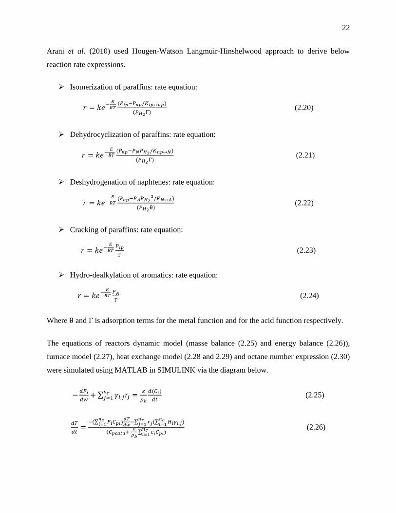
Arani et al. (2010) used Hougen-Watson Langmuir-Hinshelwood approach to derive below
reaction rate expressions.
Isomerization of paraffins: rate equation:
𝑟 = 𝑘𝑒−𝐸
𝑅𝑇(𝑃𝑖𝑝−𝑃𝑛𝑝/𝐾𝑖𝑝↔𝑛𝑝)
(𝑃𝐻2Γ) (2.20)
Dehydrocyclization of paraffins: rate equation:
𝑟 = 𝑘𝑒−𝐸
𝑅𝑇(𝑃𝑛𝑝−𝑃𝑁𝑃𝐻2/𝐾𝑛𝑝↔𝑁)
(𝑃𝐻2Γ) (2.21)
Deshydrogenation of naphtenes: rate equation:
𝑟 = 𝑘𝑒−𝐸
𝑅𝑇(𝑃𝑛𝑝−𝑃𝐴𝑃𝐻2
3/𝐾𝑁↔𝐴)
(𝑃𝐻2θ) (2.22)
Cracking of paraffins: rate equation:
𝑟 = 𝑘𝑒−𝐸
𝑅𝑇𝑃𝑖𝑝
Γ (2.23)
Hydro-dealkylation of aromatics: rate equation:
𝑟 = 𝑘𝑒−𝐸
𝑅𝑇𝑃𝐴
Γ (2.24)
Where θ and Γ is adsorption terms for the metal function and for the acid function respectively.
The equations of reactors dynamic model (masse balance (2.25) and energy balance (2.26)),
furnace model (2.27), heat exchange model (2.28 and 2.29) and octane number expression (2.30)
were simulated using MATLAB in SIMULINK via the diagram below.
−𝑑𝐹𝑖
𝑑𝑤+ ∑ 𝛾𝑖,𝑗𝑟𝑗
𝑛𝑟𝑗=1 =
𝜌𝑏
𝑑(𝐶𝑖)
𝑑𝑡 (2.25)
𝑑𝑇
𝑑𝑡=
−(∑ 𝐹𝑖𝐶𝑝𝑖)𝑑𝑇
𝑑𝑤−∑ 𝑟𝑗(∑ 𝐻𝑖𝛾𝑖,𝑗)
𝑛𝑐𝑖=1
𝑛𝑟𝑗=1
𝑛𝑐𝑖=1
(𝐶𝑝𝑐𝑎𝑡𝑎+ 𝜀
𝜌𝑏∑ 𝑐𝑖𝐶𝑝𝑖)
𝑛𝑐𝑖=1
(2.26)
23
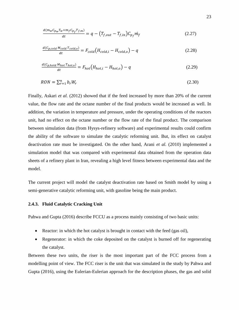
𝑑(𝑚𝑤𝐶𝑝𝑤𝑇𝑤+𝑚𝑓𝐶𝑝𝑓𝑇𝑓,𝑚)
𝑑𝑡= 𝑞 − (𝑇𝑓,𝑜𝑢𝑡 − 𝑇𝑓,𝑖𝑛)𝐶𝑝𝑓
𝑚𝑓̇ (2.27)
𝑑(𝐶𝑝,𝑐𝑜𝑙𝑑 𝑀𝑐𝑜𝑙𝑑 𝑇𝑐𝑜𝑙𝑑,𝑜)
𝑑𝑡= 𝐹𝑐𝑜𝑙𝑑(𝐻𝑐𝑜𝑙𝑑,𝑖 − 𝐻𝑐𝑜𝑙𝑑,𝑜) − 𝑞 (2.28)
𝑑(𝐶𝑝,ℎ𝑜𝑙𝑑 𝑀ℎ𝑜𝑡 𝑇ℎ𝑜𝑡,𝑜)
𝑑𝑡= 𝐹ℎ𝑜𝑡(𝐻ℎ𝑜𝑡,𝑖 − 𝐻ℎ𝑜𝑡,𝑜) − 𝑞 (2.29)
𝑅𝑂𝑁 = ∑ 𝑏𝑟𝑊𝑟𝑛𝑟=1 (2.30)
Finally, Askari et al. (2012) showed that if the feed increased by more than 20% of the current
value, the flow rate and the octane number of the final products would be increased as well. In
addition, the variation in temperature and pressure, under the operating conditions of the reactors
unit, had no effect on the octane number or the flow rate of the final product. The comparison
between simulation data (from Hysys-refinery software) and experimental results could confirm
the ability of the software to simulate the catalytic reforming unit. But, its effect on catalyst
deactivation rate must be investigated. On the other hand, Arani et al. (2010) implemented a
simulation model that was compared with experimental data obtained from the operation data
sheets of a refinery plant in Iran, revealing a high level fitness between experimental data and the
model.
The current project will model the catalyst deactivation rate based on Smith model by using a
semi-generative catalytic reforming unit, with gasoline being the main product.
2.4.3. Fluid Catalytic Cracking Unit
Pahwa and Gupta (2016) describe FCCU as a process mainly consisting of two basic units:
Reactor: in which the hot catalyst is brought in contact with the feed (gas oil),
Regenerator: in which the coke deposited on the catalyst is burned off for regenerating
the catalyst.
Between these two units, the riser is the most important part of the FCC process from a
modelling point of view. The FCC riser is the unit that was simulated in the study by Pahwa and
Gupta (2016), using the Eulerian-Eulerian approach for the description phases, the gas and solid
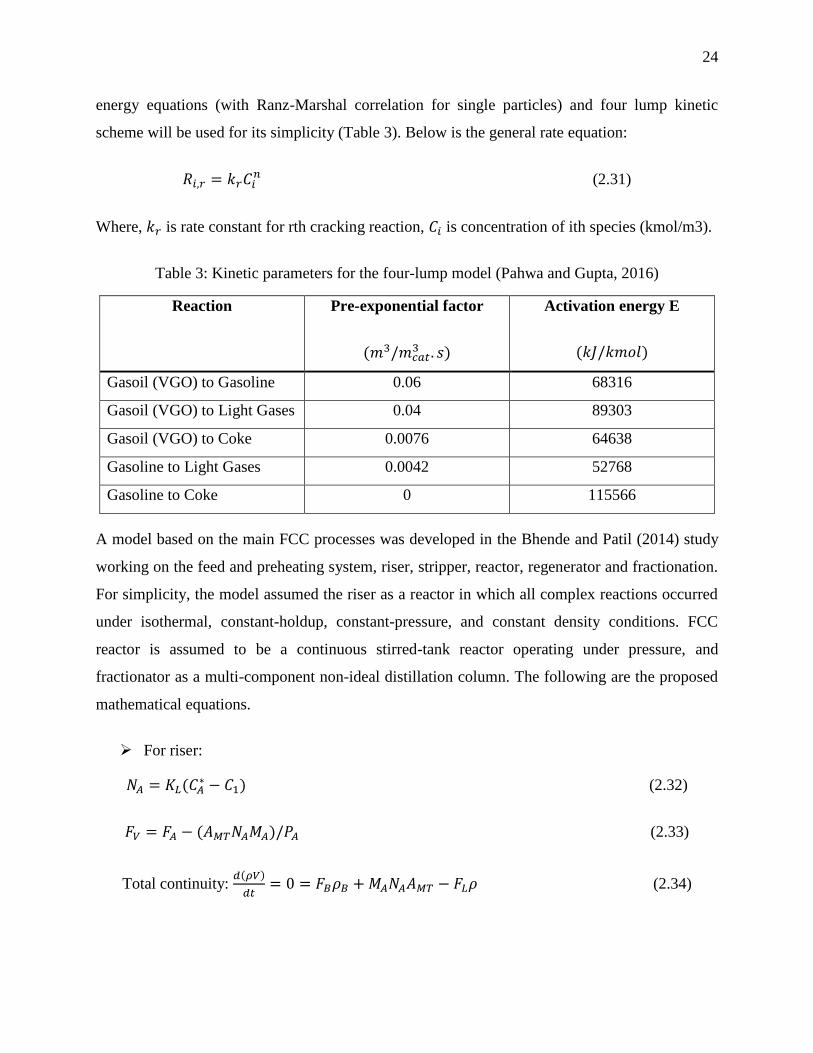
24
energy equations (with Ranz-Marshal correlation for single particles) and four lump kinetic
scheme will be used for its simplicity (Table 3). Below is the general rate equation:
𝑅𝑖,𝑟 = 𝑘𝑟𝐶𝑖𝑛 (2.31)
Where, 𝑘𝑟 is rate constant for rth cracking reaction, 𝐶𝑖 is concentration of ith species (kmol/m3).
Table 3: Kinetic parameters for the four-lump model (Pahwa and Gupta, 2016)
Reaction Pre-exponential factor
(𝑚3/𝑚𝑐𝑎𝑡3 . 𝑠)
Activation energy E
(𝑘𝐽/𝑘𝑚𝑜𝑙)
Gasoil (VGO) to Gasoline 0.06 68316
Gasoil (VGO) to Light Gases 0.04 89303
Gasoil (VGO) to Coke 0.0076 64638
Gasoline to Light Gases 0.0042 52768
Gasoline to Coke 0 115566
A model based on the main FCC processes was developed in the Bhende and Patil (2014) study
working on the feed and preheating system, riser, stripper, reactor, regenerator and fractionation.
For simplicity, the model assumed the riser as a reactor in which all complex reactions occurred
under isothermal, constant-holdup, constant-pressure, and constant density conditions. FCC
reactor is assumed to be a continuous stirred-tank reactor operating under pressure, and
fractionator as a multi-component non-ideal distillation column. The following are the proposed
mathematical equations.
For riser:
𝑁𝐴 = 𝐾𝐿(𝐶𝐴∗ − 𝐶1) (2.32)
𝐹𝑉 = 𝐹𝐴 − (𝐴𝑀𝑇𝑁𝐴𝑀𝐴)/𝑃𝐴 (2.33)
Total continuity: 𝑑(𝜌𝑉)
𝑑𝑡= 0 = 𝐹𝐵𝜌𝐵 + 𝑀𝐴𝑁𝐴𝐴𝑀𝑇 − 𝐹𝐿𝜌 (2.34)
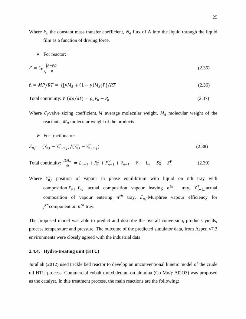
25
Where 𝑘𝐿 the constant mass transfer coefficient, 𝑁𝐴 flux of A into the liquid through the liquid
film as a function of driving force.
For reactor:
𝐹 = 𝐶𝑉√𝑃−𝑃𝐷
𝜌 (2.35)
ñ = 𝑀𝑃/𝑅𝑇 = {[𝑦𝑀𝐴 + (1 − 𝑦)𝑀𝐵]𝑃}/𝑅𝑇 (2.36)
Total continuity: 𝑉 (𝑑𝜌/𝑑𝑡) = 𝜌𝑜𝐹0 − 𝑃𝜌 (2.37)
Where 𝐶𝑉valve sizing coefficient, 𝑀 average molecular weight, 𝑀𝐴 molecular weight of the
reactants, 𝑀𝐵 molecular weight of the products.
For fractionator:
𝐸𝑛𝑗 = (𝑌𝑛𝑗 − 𝑌𝑛−1,𝑗𝑇 )/(𝑌𝑛𝑗
∗ − 𝑌𝑛−1,𝑗𝑇 ) (2.38)
Total continuity: 𝑑(𝑀𝑛)
𝑑𝑡= 𝐿𝑛+1 + 𝐹𝑛
𝐿 + 𝐹𝑛−1𝑉 + 𝑉𝑛−1 − 𝑉𝑛 − 𝐿𝑛 − 𝑆𝑛
𝐿 − 𝑆𝑛𝑉 (2.39)
Where 𝑌𝑛𝑗∗ position of vapour in phase equilibrium with liquid on nth tray with
composition 𝑋𝑛𝑗, 𝑌𝑛𝑗 actual composition vapour leaving 𝑛𝑡ℎ tray, 𝑌𝑛−1,𝑗𝑇 actual
composition of vapour entering 𝑛𝑡ℎ tray, 𝐸𝑛𝑗 Murphree vapour efficiency for
𝑗𝑡ℎcomponent on 𝑛𝑡ℎ tray.
The proposed model was able to predict and describe the overall conversion, products yields,
process temperature and pressure. The outcome of the predicted simulator data, from Aspen v7.3
environments were closely agreed with the industrial data.
2.4.4. Hydro-treating unit (HTU)
Jurallah (2012) used trickle bed reactor to develop an unconventional kinetic model of the crude
oil HTU process. Commercial cobalt-molybdenum on alumina (Co-Mo/γ-Al2O3) was proposed
as the catalyst. In this treatment process, the main reactions are the following:
26
Hydrodesulphurization (HDS), hydrodenitrogenation (HDN), hydrodeasphaltenization (HDAs),
hydrodemetallization (HDM), that include hydrodevanadization or HDV and hydrodenickelation
or HDNi).
HDs: 𝑅 − 𝑆 + 𝐻2 → 𝑅 + 𝐻2𝑆 (Reaction 4)
HDN: 𝑅 − 𝑁𝐻2 + 𝐻2 → 𝑅𝐻 + 𝑁𝐻3 (Reaction 5)
HDM: 𝑅 − 𝑀 + 𝐻2 → 𝑅𝐻 + 𝑀 (Reaction 6)
HDAs: 𝑅 − 𝐴𝑠𝑝ℎ + 𝐻2 → 𝑅𝐻 + 𝐴𝑠𝑝ℎ − 𝑅(𝑠𝑚𝑎𝑙𝑙𝑒𝑟 ℎ𝑦𝑑𝑟𝑜𝑐𝑎𝑟𝑏𝑜𝑛𝑠) (Reaction 7)
R represents the hydrocarbon molecule.
The general process modelling system (gPROMS) was used to model and simulate the process
using below equations, based on:
Mass balance equations in gas phase:
Hydrogene:𝑑𝑃𝐻2
𝐺
𝑑𝑧= −
𝑅𝑇
𝑢𝑔𝑘𝐻2
𝐿 𝑎𝐿(𝑃𝐻2
𝐺
ℎ𝐻2
− 𝐶𝐻2
𝐿 ) (2.40)
𝐻2𝑆: 𝑑𝑃𝐻2
𝐺
𝑑𝑧= −
𝑅𝑇
𝑢𝑔𝑘𝐻2
𝐿 𝑎𝐿(𝑃𝐻2𝑆
𝐺
ℎ𝐻2𝑆− 𝐶𝐻2𝑆
𝐿 ) (2.41)
Mass balance equations in liquid phase:
Hydrogene:𝑑𝐶𝐻2
𝐿
𝑑𝑧=
1
𝑢𝑙[𝑘𝐻2
𝐿 𝑎𝐿 (𝑃𝐻2
𝐺
ℎ𝐻2
− 𝐶𝐻2
𝐿 ) − 𝑘𝐻2
𝑆 𝑎𝑠(𝐶𝐻2
𝐿 − 𝐶𝐻2
𝑆 )] (2.42)
𝐻2𝑆:𝑑𝐶𝐻2𝑆
𝐿
𝑑𝑧=
1
𝑢𝑙[𝑘𝐻2𝑆
𝐿 𝑎𝐿 (𝑃𝐻2𝑆
𝐺
ℎ𝐻2𝑆− 𝐶𝐻2𝑆
𝐿 ) − 𝑘𝐻2𝑆𝑆 𝑎𝑠(𝐶𝐻2𝑆
𝐿 − 𝐶𝐻2𝑆𝑆 )] (2.43)
𝑑𝐶𝑖𝐿
𝑑𝑧= −
1
𝑢𝑙𝑘𝑖
𝑆𝑎𝑠(𝐶𝑖𝐿 − 𝐶𝑖
𝑆) (2.44)
Where 𝑖 = sulfur, nitrogen, asphaltene, vanadium or nickel
Mass balance equations in solid phase:
27
Hydrogene:𝑘𝐻2
𝑆 𝑎𝑠(𝐶𝐻2
𝐿 − 𝐶𝐻2
𝑆 ) = 𝜌𝐵 ∑ 𝜂𝑗 𝑟𝑗 (2.45)
𝐻2𝑆:𝑘𝐻2𝑆𝑆 𝑎𝑠(𝐶𝐻2𝑆
𝐿 − 𝐶𝐻2𝑆𝑆 ) = −𝜌𝐵𝜂𝐻𝐷𝑆𝑟𝐻𝐷𝑆 (2.46)
𝑘𝑖𝑆𝑎𝑠(𝐶𝑖
𝐿 − 𝐶𝑖𝑆) = −𝜌𝐵𝜂𝑖𝑟𝑖 (2.47)
Where 𝑖 = sulfur, nitrogen, asphaltene, vanadium or nickel and 𝑗 = HDS, HDN, HDAs, HDV and
HDNi.
Daneshvar and Fatemi (2011) presented a non-isothermal three-phase heterogeneous model to
describe the hydro-treatment of diesel in a trickle-bed reactor. The model was based on mass
balance equations in gas phase (H2, H2S andNH3), liquid phase (S, A, NB, NNBand HC) and
solide phase (for HDS, HDN and HDAs reactions), energy balance and chemical reaction
kinetics (2.48, 2.49, 2.50, 2.51, 2.52, 2.53) as proposed by Jurallah (2011).
Korsten and Hoffmann: 𝑟𝐻𝐷𝑆 = 𝐾𝐻𝐷𝑆
(𝐶𝑆𝑆)(𝐶𝐻2
𝑆 )0.45
(1+ 𝐾𝐻2𝑆𝐶𝐻2𝑆𝑆 )2 (2.48)
Murali and Voolapalli: 𝑟𝐻𝐷𝑆 = 𝐾𝐻𝐷𝑆
(𝐶𝑆𝑆)1.64(𝐶𝐻2
𝑆 )0.55
(1+ 𝐾𝐻2𝑆𝐶𝐻2𝑆𝑆 )2 (2.49)
Cheng and Fang: 𝑟𝐻𝐷𝑆 = 𝐾𝐻𝐷𝑆
(𝐶𝑆𝑆)2(𝐶𝐻2
𝑆 )0.6
1+ 𝐾𝐻2𝑆𝐶𝐻2𝑆𝑆 (2.50)
Non-basic (HDN): 𝑟𝐻𝐷𝑁𝑁𝐵= 𝑘𝐻𝐷𝑁𝑁𝐵
(𝐶𝑁𝑁𝐵
𝑆 )1.5 (2.51)
Basic (HDN): 𝑟𝐻𝐷𝑁𝑁𝐵= 𝑘𝐻𝐷𝑁𝑁𝐵
(𝐶𝑁𝑁𝐵
𝑆 )1.5 − 𝑘𝐻𝐷𝑁𝐵(𝐶𝑁𝐵
𝑆 )1.5 (2.52)
Forward and reverse reaction (HDA): 𝑟𝐻𝐷𝑁𝑁𝐵= 𝑘𝑓𝑝𝐻2
𝐺 𝐶𝐴𝑆 − 𝑘𝑟(1 − 𝐶𝐴
𝑆) (2.53)
The model of Murali and Voopalli was consistent with experimental results compared with other
kinetics models of HDS.
28
2.5. Environmental aspects of refinery production
According to I.E.A. (2016) South Africa recorded a 60.3% increase in the production of 𝐶𝑂2
from fuel oil combustion, resulting in an increase of 27.8 million tons in 1971 to 69.1 million
tons, between 1990 and 2014. Although South Africa accounted for 38% of 𝐶𝑂2 emissions from
fuel combustion throughout Africa in 2011, this represented only 1% of the global total. This
position is largely due to the economy’s dependence on fossil fuels, especially the electricity and
heating sector. In addition, according to Naré and Kamakaté (2017), road transport is one of the
leading sources of outdoor air pollution in Western and Southern Africa due to the use of
vehicles. In fact, for transport of people and goods in Sub-Saharan Africa, motor vehicles are
increasingly used (Thambiran and Diab, 2011). Large vehicle emissions result from rapid
urbanization and motorization makes cities pollution hotspots.
Figure 5: South African CO2 Emissions (Metric tons per capita) per year
Source: (World Bank Group, 2012)
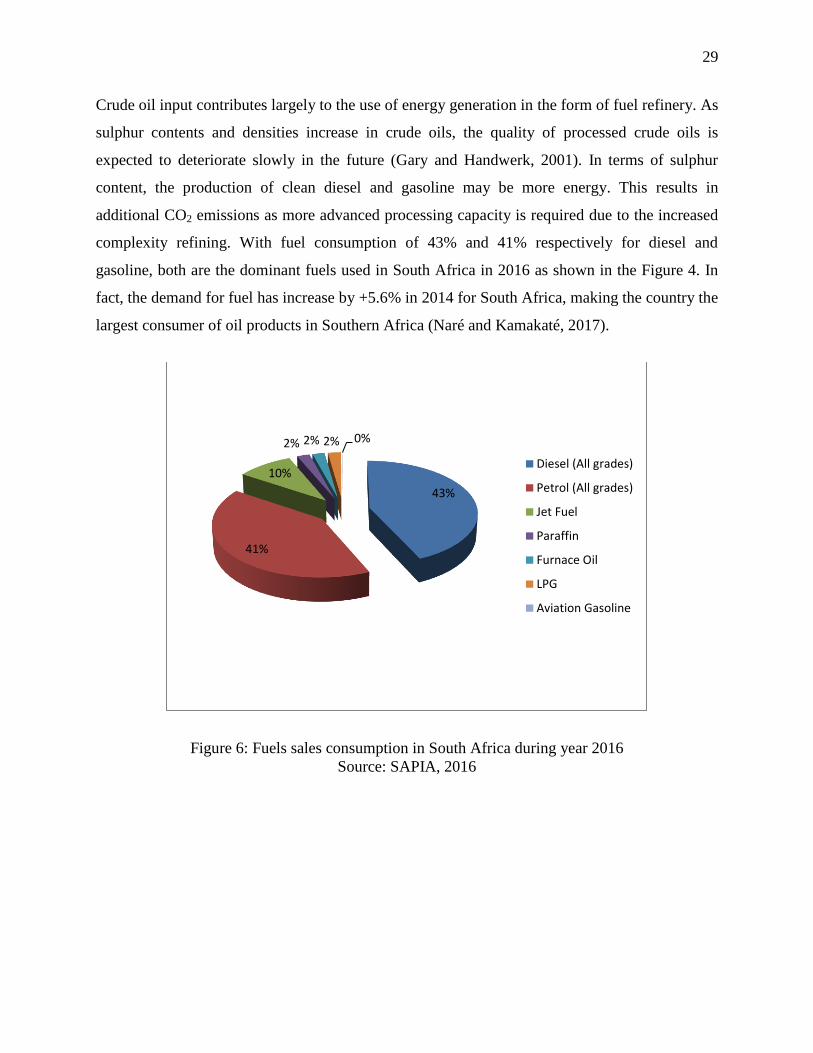
29
Crude oil input contributes largely to the use of energy generation in the form of fuel refinery. As
sulphur contents and densities increase in crude oils, the quality of processed crude oils is
expected to deteriorate slowly in the future (Gary and Handwerk, 2001). In terms of sulphur
content, the production of clean diesel and gasoline may be more energy. This results in
additional CO2 emissions as more advanced processing capacity is required due to the increased
complexity refining. With fuel consumption of 43% and 41% respectively for diesel and
gasoline, both are the dominant fuels used in South Africa in 2016 as shown in the Figure 4. In
fact, the demand for fuel has increase by +5.6% in 2014 for South Africa, making the country the
largest consumer of oil products in Southern Africa (Naré and Kamakaté, 2017).
Figure 6: Fuels sales consumption in South Africa during year 2016
Source: SAPIA, 2016
43%
41%
10%
2% 2% 2% 0%
Diesel (All grades)
Petrol (All grades)
Jet Fuel
Paraffin
Furnace Oil
LPG
Aviation Gasoline
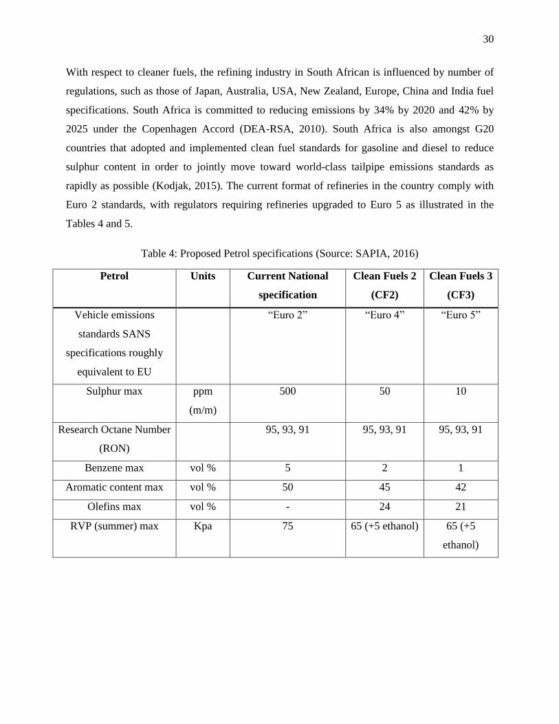
30
With respect to cleaner fuels, the refining industry in South African is influenced by number of
regulations, such as those of Japan, Australia, USA, New Zealand, Europe, China and India fuel
specifications. South Africa is committed to reducing emissions by 34% by 2020 and 42% by
2025 under the Copenhagen Accord (DEA-RSA, 2010). South Africa is also amongst G20
countries that adopted and implemented clean fuel standards for gasoline and diesel to reduce
sulphur content in order to jointly move toward world-class tailpipe emissions standards as
rapidly as possible (Kodjak, 2015). The current format of refineries in the country comply with
Euro 2 standards, with regulators requiring refineries upgraded to Euro 5 as illustrated in the
Tables 4 and 5.
Table 4: Proposed Petrol specifications (Source: SAPIA, 2016)
Petrol Units Current National
specification
Clean Fuels 2
(CF2)
Clean Fuels 3
(CF3)
Vehicle emissions
standards SANS
specifications roughly
equivalent to EU
“Euro 2” “Euro 4” “Euro 5”
Sulphur max ppm
(m/m)
500 50 10
Research Octane Number
(RON)
95, 93, 91 95, 93, 91 95, 93, 91
Benzene max vol % 5 2 1
Aromatic content max vol % 50 45 42
Olefins max vol % - 24 21
RVP (summer) max Kpa 75 65 (+5 ethanol) 65 (+5
ethanol)
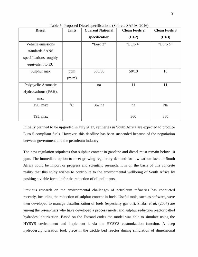
31
Table 5: Proposed Diesel specifications (Source: SAPIA, 2016)
Diesel Units Current National
specification
Clean Fuels 2
(CF2)
Clean Fuels 3
(CF3)
Vehicle emissions
standards SANS
specifications roughly
equivalent to EU
“Euro 2” “Euro 4” “Euro 5”
Sulphur max ppm
(m/m)
500/50 50/10 10
Polycyclic Aromatic
Hydrocarbons (PAH),
max
na 11 11
T90, max
T95, max
oC 362 na na
360
Na
360
Initially planned to be upgraded in July 2017, refineries in South Africa are expected to produce
Euro 5 compliant fuels. However, this deadline has been suspended because of the negotiation
between government and the petroleum industry.
The new regulation stipulates that sulphur content in gasoline and diesel must remain below 10
ppm. The immediate option to meet growing regulatory demand for low carbon fuels in South
Africa could be import or progress and scientific research. It is on the basis of this concrete
reality that this study wishes to contribute to the environmental wellbeing of South Africa by
positing a viable formula for the reduction of oil pollutants.
Previous research on the environmental challenges of petroleum refineries has conducted
recently, including the reduction of sulphur content in fuels. Useful tools, such as software, were
then developed to manage desulfurization of fuels (especially gas oil). Shakri et al. (2007) are
among the researchers who have developed a process model and sulphur reduction reactor called
hydrodesulphurization. Based on the Fotrand codes the model was able to simulate using the
HYSYS environment and implement it via the HYSYS customization function. A deep
hydrodesulphurization took place in the trickle bed reactor during simulation of dimensional
32
model of heterogeneous reactor. The study consisted of two sections: based on Hougen Watson
rate, the first was a simulation of hydrodesulphurization of a trickle bed reactor and a simulation
of the hydrodesulphurization process, based on the design and implementation of the
hydrodesulphurization model. As results of simulation, a ratio of H2/Oil equal to 55.7 gave a
better performance and the increase in temperature highly affected the sulphur concentration.
De la Paz-Zavala et al. (2013) have developed a kinetic model of hydrodesulphurization of
diesel. The objective was to reach a low sulphur diesel and apply it to commercial units.
Commercial catalysts, straight run gasoil, light cycle oil, light cracked gasoil and feedstock
proprieties were experimental data used for modelling. Simulation analysis, based on
temperature, space velocity and pressure, of the model obtained in order to compare predictions
and industrial applications.
Another study that dealing with sulphur problems in transport fuels (road and air) was published
in 2003 by Song. This study provided an insight into new contributions to deep desulfurization of
refinery streams without lower octane number or gasoline loss. Two streams were targeted:
gasoline for a reduction of 330 to 30 ppm and gasoline for a reduction of 500 to less than 15
ppm. In conclusion, Song stated that new and more effective approaches, catalyst studies and
processing researches are needed for the production of ultra-clean and affordable fuels, in line
with government regulations.
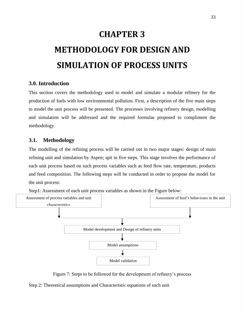
33
CHAPTER 3
METHODOLOGY FOR DESIGN AND
SIMULATION OF PROCESS UNITS
3.0. Introduction
This section covers the methodology used to model and simulate a modular refinery for the
production of fuels with low environmental pollution. First, a description of the five main steps
to model the unit process will be presented. The processes involving refinery design, modelling
and simulation will be addressed and the required formulas proposed to compliment the
methodology.
3.1. Methodology
The modelling of the refining process will be carried out in two major stages: design of main
refining unit and simulation by Aspen; spit in five steps. This stage involves the performance of
each unit process based on such process variables such as feed flow rate, temperature, products
and feed composition. The following steps will be conducted in order to propose the model for
the unit process:
Step1: Assessment of each unit process variables as shown in the Figure below:
Figure 7: Steps to be followed for the development of refinery’s process
Step 2: Theoretical assumptions and Characteristic equations of each unit
Assessment of feed’s behaviours in the unit Assessment of process variables and unit
characteristics
Model development and Design of refinery units
Model assumptions
Model validation
34
Step 3: Process modelling
Step 4: Process simulation using Aspen
Step 5: Case studies and model validations
3.2. Modular refinery design basis and Process description
a) Crude oil Distillation Unit
To design the modular refinery, this project assumed that the feed of crude oil was preheated,
desalted, heated in the furnace and then fed to the distillation unit. Fractionation takes place in
the atmospheric column (ADU) purposed to obtain: Off gas (LPG), naphtha, kerosene,
atmospheric gasoil, diesel and the atmospheric residue. The last component made of long carbon
chained molecules with high boiling points will be further fractionated in the vacuum distillation
column (VDU) into light, heavy gasoil and vacuum residue.
- Process design
Desalting design
In order to remove water and soluble salts from oil stream, desalting plants are often installed in
crude oil production units (Vafajoo, Ganjian and Fattahi, 2012).
Gravitational separation is the commonly used method to separate oil and water; this is also
applied to the electrostatic desalter which relies mainly on gravity separation governed by Stokes
law (Dreher, 2016). An expression describing the settling velocity of spherical sediments in a
fluid medium:
𝑣 =2𝑟2∆𝜌 𝑔
9𝜇0 (3.1)
where v: settling rate, kg/s/m2
𝑟: drop radius, m
∆𝜌: density difference between aqueous and organic phases, kg/m3
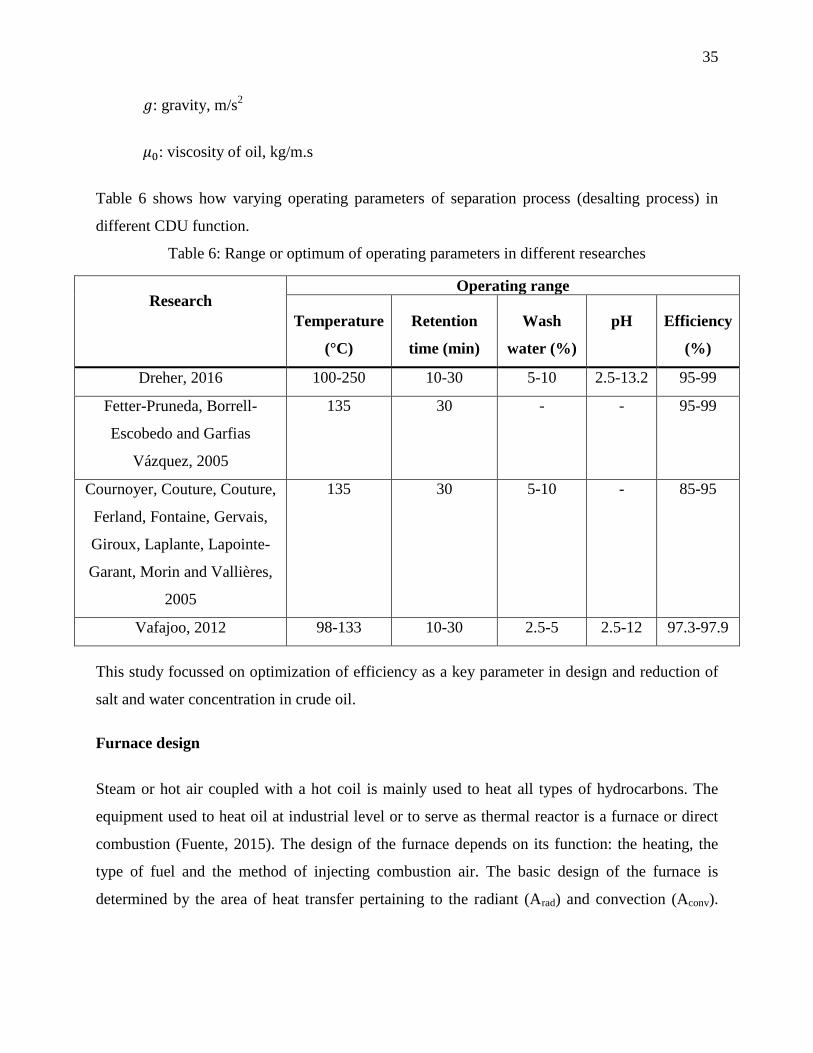
35
𝑔: gravity, m/s2
𝜇0: viscosity of oil, kg/m.s
Table 6 shows how varying operating parameters of separation process (desalting process) in
different CDU function.
Table 6: Range or optimum of operating parameters in different researches
Research Operating range
Temperature
(°C)
Retention
time (min)
Wash
water (%)
pH Efficiency
(%)
Dreher, 2016 100-250 10-30 5-10 2.5-13.2 95-99
Fetter-Pruneda, Borrell-
Escobedo and Garfias
Vázquez, 2005
135 30 - - 95-99
Cournoyer, Couture, Couture,
Ferland, Fontaine, Gervais,
Giroux, Laplante, Lapointe-
Garant, Morin and Vallières,
2005
135 30 5-10 - 85-95
Vafajoo, 2012 98-133 10-30 2.5-5 2.5-12 97.3-97.9
This study focussed on optimization of efficiency as a key parameter in design and reduction of
salt and water concentration in crude oil.
Furnace design
Steam or hot air coupled with a hot coil is mainly used to heat all types of hydrocarbons. The
equipment used to heat oil at industrial level or to serve as thermal reactor is a furnace or direct
combustion (Fuente, 2015). The design of the furnace depends on its function: the heating, the
type of fuel and the method of injecting combustion air. The basic design of the furnace is
determined by the area of heat transfer pertaining to the radiant (Arad) and convection (Aconv).
36
The sum of these two areas results in the total area of a furnace (Fuente, 2015). In order to
determine the radiant and convection area, the following equations was used (Fuente, 2015):
𝐴𝑟𝑎𝑑 =0.5 𝑄
𝑞𝑟 (3.2)
𝐴𝑐𝑜𝑛 =0.5 𝑄
𝑞𝑐 (3.3)
where 𝑞𝑟: The heat flux in the radiant section is, quantified as 37.6 kW/m2
𝑞𝑐 : The heat flux which occurs in the convection section, quantified as 12.5 kW/m2
𝑄 : The heat required by the inlet cold stream to reach the desired temperature or
absorbed duty from heat balance or heat duty desired temperature
In this study the design of the use of furnace was adopted from Fuente, (2015) as indicated in the
literature above.
Heat exchanger design
The design of heat exchanger is used in the pre-heating unit, as device used to transfer heat
between a solid object and a fluid, or between two or more fluids.
According to Kemp (2007), the Equation 3.4 which represents a simple equation that calculates
the ΔT for heat exchanger matches, is quite useful for gases and viscous liquids with poor overall
heat transfer coefficients (U), or fouling heat exchanger surfaces. It is the general formula that
describes the heat transfer (Q) which occurs through heat exchangers and gives a better value for
the ΔT for such fluids (Kemp, 2007; Sinnot, 2005, Fuente, 2015).
𝑄 = 𝑈𝐴∆𝑇𝑀 (3.4)
where 𝑄 : Heat transfer rate [W] : From the energy balance
𝑈 : Overall transfer coefficient [W/ (m2.K)]: Estimation of heat transfer coefficient which
depends on configuration and media used in the Shell and Tube side: L-L, Condensing
vapour-L, Gas-L, Vaporizers. Selected from Backhurst, Coulson, Harker, and Richardson
(1999).
𝐴 : Heat transfer surface area [m2]
∆TM: mean temperature difference [K]
∆TM = 𝐹𝑇∆𝑇𝐿𝑀 (3.5)
37
where 𝐹𝑇: Factor used to correct the departure from true counter current flow
∆𝑇𝐿𝑀 : Log mean temperature difference ∆𝑇𝑀, K
∆𝑇𝐿𝑀 =(𝑇1−𝑡2)−(𝑇2−𝑡1)
ln(𝑇1−𝑡2𝑇2−𝑡1
) (3.6)
where 𝑇1: Hot stream inlet temperature [K]
𝑇2: Hot stream outlet temperature [K]
𝑡1: Cold stream inlet temperature [K]
𝑡2: Cold stream outlet temperature [K]
It is important to note that ∆𝑇𝐿𝑀 is the logarithmic average of the temperature difference
between the hot and cold streams at each end of the exchanger and has a direct correlation on the
amount of heat transferred for a counter current flow heat exchanger.
The parameter calculated and used in this study is the area, which was the main parameter for
simulation.
Distillation column design
Feeding location, number of trays or column diameter, trays design or packing type, distance
between trays or packings height, total column height, operating conditions, and mechanical
design are some of the parameters required for complete design and optimization of distillation.
Among these parameters, the determination of the theoretical stages and the feed location are one
of the first steps in distillation design (Green and Perry, 2007; Caballero, 2014).
The crude oil column design requires some input data such as crude oil true boiling point (TBP),
density or API gravity, molecular weight and viscosity, as well as required specifications such as
column pressure. Product specification can be determined in terms of fix or distillation point,
pumping around entitlements and column top temperature (Pant and Kunzru, 2015).
The process design of distillation column includes the following steps: specify the separation and
determination of the material and energy balance optimization; set a column pressure; determine
the minimum reflux and the minimum number of stages; find the optimal feeding stage; Select
three ratios of actual reflux preceding minimum reflux (Kister, 1992). Calculations during
process design can be abridged or rigorous, it is therefore important to re-exanimate some steps
38
and to graphically analyze the design. This procedure ensures optimal design and the absence of
pinched regions (Kister, 1992).
Most distillation processes in industry are used to separate more than two components. As in the
case of distillation of two components, the same type of distillation columns, reboilers,
condensers, heat exchangers and so on, is used on multicomponent separations. The cuts
obtained after distillation are called key components among which the light key (LK), heavy key
(HK) and other components called non-keys (NK) exist. The process also produces light non-key
(LNK), more volatile non-key, and the heavy non-key (HNK), less volatile heavy key
(Manjumdor and Das, 2012). The design process consists of calculation steps in the distillation
of multicomponent systems, which is performed using several short-cut methods. These
generally involve an estimation of the following parameters: minimum number of trays,
minimum reflux rate and the number of stages (Manjumdor and Das, 2012; Ibrahim, 2014). A
widely used approximate method is commonly referred to as the Fenske-Underwood-Gilliland
method or FUG (Manjumdor and Das, 2012).
This study relates to a distillation that contains inter alia atmospheric distillation as a vacuum
distillation unit in two different columns. So, the design of the columns is therefore focused on
the calculations of the following parameters (Douglas, 1998; McCabe and Warren, 1993).
Determination of process operations variables :
Some parameters such as feed rate, composition, purity of the distillate and the bottom, and
quality of the feed are assumed to be known. Determination of the distillate and bottoms is done
by oerforming overall material and component balances.
𝐹 𝑍𝐹 = 𝑋𝐷𝐷 + 𝑋𝐵𝐵 (3.7)
𝐹 = 𝐷 + 𝐵 (3.8)
where, 𝐹: Feed rate of input stream
𝑍𝐹: Composition of light component in feed
𝑋𝐷: Mole fraction of light component in distillate
𝑋𝐵: Mole fraction of light component in bottom
𝐷: Total distillate amount
39
𝐵: Total bottom amount
As crude oil contains more than two components, 𝑋𝐷 and 𝑋𝐵are light-key and heavy-key
component.
Determination of minimum reflux ratio
The determination of minimum reflux ratio is done either analytically, using Underwood
Equations, or graphically, using the McCabe-Thiele method.
The use of the McCabe-Thiele method implies the following assumptions: constant molar
overflow; heat effects are negligible; for every mole of vapour condensed, another mole of liquid
is vaporized; and the liquid and vapour leaving the tray is in equilibrium with the vapour and
liquid entering the tray (Douglas, 1988). A diagram Y-X (Y representing the vapour phase and X
the liquid) is plotted if no equilibrium curve is given, which can be can be obtained by relating
the relative volatility (𝛼) to the composition of the liquid (McCabe and Warren, 1993):
𝑌 =𝛼𝑋
1+(𝛼−1)𝑋 (3.9)
This shows the bubble-point and dew point of a binary mixture at constant pressure. An
equilibrium line describes the compositions of the liquid and vapour in equilibrium at a fixed
pressure.
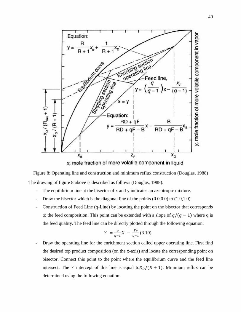
40
Figure 8: Operating line and construction and minimum reflux construction (Douglas, 1988)
The drawing of figure 8 above is described as follows (Douglas, 1988):
- The equilibrium line at the bisector of x and y indicates an azeotropic mixture.
- Draw the bisector which is the diagonal line of the points (0.0,0.0) to (1.0,1.0).
- Construction of Feed Line (q-Line) by locating the point on the bisector that corresponds
to the feed composition. This point can be extended with a slope of 𝑞/(𝑞 − 1) where q is
the feed quality. The feed line can be directly plotted through the following equation:
𝑌 = 𝑞
𝑞−1𝑋 −
𝑍𝐹
𝑞−1 (3.10)
- Draw the operating line for the enrichment section called upper operating line. First find
the desired top product composition (on the x-axis) and locate the corresponding point on
bisector. Connect this point to the point where the equilibrium curve and the feed line
intersect. The 𝑌 intercept of this line is equal to𝑋𝐷/(𝑅 + 1). Minimum reflux can be
determined using the following equation:
41
𝑅𝑚𝑖𝑛 =𝑋𝐷
𝑌𝑖𝑛𝑡𝑒𝑟𝑐𝑒𝑝𝑡− 1 (3.11)
- Draw the operating line for the stripping section called lower operating line. First find the
desired bottom product composition (on the x-axis) and locate the corresponding point on
bisector. Draw a line from this point at the intersection of the equilibrium curve and the
feed line. The slope of this line is equal to 𝑉𝑏𝑚𝑖𝑛/(𝑅 + 1); where 𝑉𝑏𝑚𝑖𝑛 is the boiling
point, corresponding to the minimum reflux of the fractional amount of liquid returned to
the column of liquid leaving.
Determination of the actual reflux ratio
The distillation columns are mostly designed to operate between 1.2 and 1.5 times the minimum
reflux ratio because this range corresponds approximately to the zone of minimum operating
cost. Based on the first estimates, the operating reflux is therefore equated as following
(Douglas, 1998):
𝑅𝑎𝑐𝑡𝑢𝑎𝑙 = 1.2 𝑅𝑚𝑖𝑛 (3.12)
𝑅 = 𝐿/𝐷 (3.13)
Analytically, the minimum reflux ratio is approximated by the Underwood equation as stated
above (Douglas, 1988). With respect to mass balances and VLE equations, the following
equation can be used for multi-component systems with constant relative volatility and ∅ can
be calculated derived from the equation.
𝑭(𝟏 − 𝒒) = ∑((𝜶𝒊 𝒛𝒊)/ (𝜶𝒊 − ∅)) (3.14)
where 𝑭 : Feed
𝒒 : Feed quality
𝜶𝒊 : Relative Volatility
𝒛𝒊 : Composition of component (i) in Feed
Considering the equation (3.14), ∅ can be obtained in a polynomial expression. This expression
can be used to solve for ∅. Only ∅ between the relative volatilities of the components should be
considered. The ∅ can be used to get the minimum amount of vapour (𝑉𝑚𝑖𝑛):
42
𝑽𝒎𝒊𝒏 = ∑((𝜶𝒊 𝑫𝒙𝒊)/ (𝜶𝒊 − ∅)) (3.15)
From a mass balance and the definition of reflux:
𝑳𝒎𝒊𝒏 = 𝑽𝒎𝒊𝒏 – 𝑫 (3.16)
𝑹𝒎𝒊𝒏 = 𝑽𝒎𝒊𝒏 / 𝑫 (3.17)
Determination of the minimum number of trays and theoretical number of trays
The upper and lower operating line and the actual reflux ratio can be used to determine the
number of trays. From the plotting point to 𝑋𝐷/(𝑅 + 1) and from the line plot 𝑋𝐷, the equation
of the upper line is:
𝑌 =𝑅
𝑅+1𝑋 +
𝑋𝐷
𝑅+1 (3.18)
By connecting the point to 𝑋𝐵to the intersection of the feed line and the upper line, the equation
of the lower operating line can be drawn:
𝑌 =𝑉𝐵+1
𝑉𝐵𝑋 +
𝑋𝐵
𝑉𝐵 (3.19)
From composition of the distillate (projection of 𝑋𝐷 on the forty Five Degree line), the horizontal
is drawn to the equilibrium curve. This line represents the first tray. From intersection of the
previous horizontal line and the equilibrium curve, drop vertically until the upper operating line
is obtained. As for the first horizontal a second horizontal is drawn to determine the next tray.
Continue doing same operation until the liquid compositions ends the desired bottom
composition. The theoretical number of trays is equal to the total numbers of steps.
Analytically, a simplified approximate equation can be used to determine the number of trays.
Fenske is an expression of the minimum number of trays, assuming total reflux and constant
relative volatility. This equation takes into account the reflux ratio (Douglas, 1988).
𝑁 =ln 𝑆𝐹
ln(𝛼
√(1+1/𝑅∗𝑍𝐹)) (3.20)
43
where:
𝑆𝐹 = 𝛽 ∗𝛿
((1−𝛿)∗(1−𝛽)) (3.21)
𝛽: Fractional recovery of light in the distillate
𝛿: Fractional recovery of light in the bottom
𝛼: Relative volatility
𝑅: Reflux ratio
𝑍𝐹: Mole ratio of light component in feed
Determination of the actual number of trays
The actual number of trays is determined by taking the quotient of the number of theoretical
trays to the tray efficiency in the range of 0.5 to 0.7. These values depend on the type of trays
used and the internal flow rate of liquid and vapour (Douglas, 1998):
𝑁𝑎𝑐𝑡𝑢𝑎𝑙 = 𝑁𝑡ℎ𝑒𝑜𝑟𝑦/휀 (3.22)
Determination of principal dimensions of the column (Diameter/Height):
According to the design guideline, the height of the column should not exceed 60m (Price,
2003). The ratio of height to diameter ratio should be less than 20 to 30 (Douglas, 1988).
The tower height may be related to the number of trays in the column. The formula below
indicates that a gap of 0.61 m between trays will be sufficient, which includes an additional 1.52
to 3.05 m at both ends of the tower; this will includes a 15% excess allowance of space (Douglas,
1988):
𝐻𝑡𝑜𝑤𝑒𝑟 = 2.3 𝑁𝑎𝑐𝑡𝑢𝑎𝑙 (3.23)
The diameter of a tower is relatively insensitive to changes in operating temperature or pressure.
Determination of the column diameter needs to consider the vapour velocity (𝑉) which is the
main determinant of the diameter and can be derived from the flooding velocity. A velocity 50-
44
80% of flooding is chosen to limit column from as stated by Douglas. The desired vapour
velocity is dependent on the limitations of undesired column flooding. This equation allows for a
twelve % surplus in area (Douglas, 1998):
𝐷𝑇 = 0.0164 √𝑉 (𝑀𝐺
𝜌𝑚)0.25 (3.24)
where
𝑉 =1.2
√𝜌𝐺 (3.25)
𝐷𝑇: Diameter of the tower
𝑉: Vapour velocity
𝑀𝐺: Molecular weight of gas
𝜌𝑚: Molar density
𝜌𝐺: Density of the mixture
b) Fluid Catalytic Cracking Unit
- Process description
The FCCU includes preheating the feed, feed nozzles, riser, catalyst separation, striping
section and regenerator valves. From CDU and VDU, the feed of FCCU passes through a
vertical riser reactor where cracking reactions are carried out. The oil fed into this unit moves
up in the riser, vaporizes and cracks at the same time to lighter products, carrying the catalyst
powder along with it. The catalyst used is a zeolite which flows like a liquid because the
pressure force is transmitted through the catalyst particles (Sadeghbeigi, 2000). The products
in this unit are light gases, gasoline products and coke. The coke deposited on the catalyst
and both are separated in the regenerator.
- Process design
There are different reactors used for catalytic cracking such as three-phase fluidized bed reactor
(using an upward flow of liquid as opposed to the gas), the continuous stirred tank reactor (for
homogeneous reactions), the fixed/packed bed reactor and the fluidized bed reactor. The
45
fluidized bed reactor is the suitable for conversion of gas oils into gasoline. It allows
regeneration of the short lifespan catalyst and offers better loss of catalyst.
In this study, the choice of the fluidized bed reactor takes into account the fact that the most
appropriate option is the conversion of gasoil into gasoline. This is the essential part serving as
the reactor in the FCC is the riser. The configuration of this reactor is vital to maintain the FCC
pressure balance (Sadeghbeigi, 2000).
The riser temperature, catalyst flow rate, feed catalyst temperature and catalyst to oil ratio (COR)
are parameters to be optimized in this section so the design focuses only on the catalyst.
- Catalyst design
The catalyst design consists of calculating the weight and deactivation, as well as catalysts
parameter and specifications as follows:
Mass of the catalyst at any given time is given as follows:
𝑚𝑐𝑎𝑡 = 𝜌𝐶𝑎𝑡𝑉𝑐𝑎𝑡 (3.26)
where:
𝑉𝐶𝑎𝑡 = 𝑡𝑐𝑄𝑐𝑎𝑡 (3.27)
𝜌𝐶𝑎𝑡: Density of the catalyst
𝑉𝐶𝑎𝑡: Volume (flowrate) of the catalyst
𝑡𝐶: Residence time
𝑄𝑐𝑎𝑡: Flow rate of catalyst
Knowing that the amount of catalyst circulating between the regenerator and the reactor is about
5 kg of feedstock (i.e 4.66 kg per litre of feed stream) (Gary and Handwerk, 2007); and having
determined the feed flow rate, the bulk catalyst mass per day can be determined. Also, the
residence time is taken equal to 2 seconds according to Lee (2016).
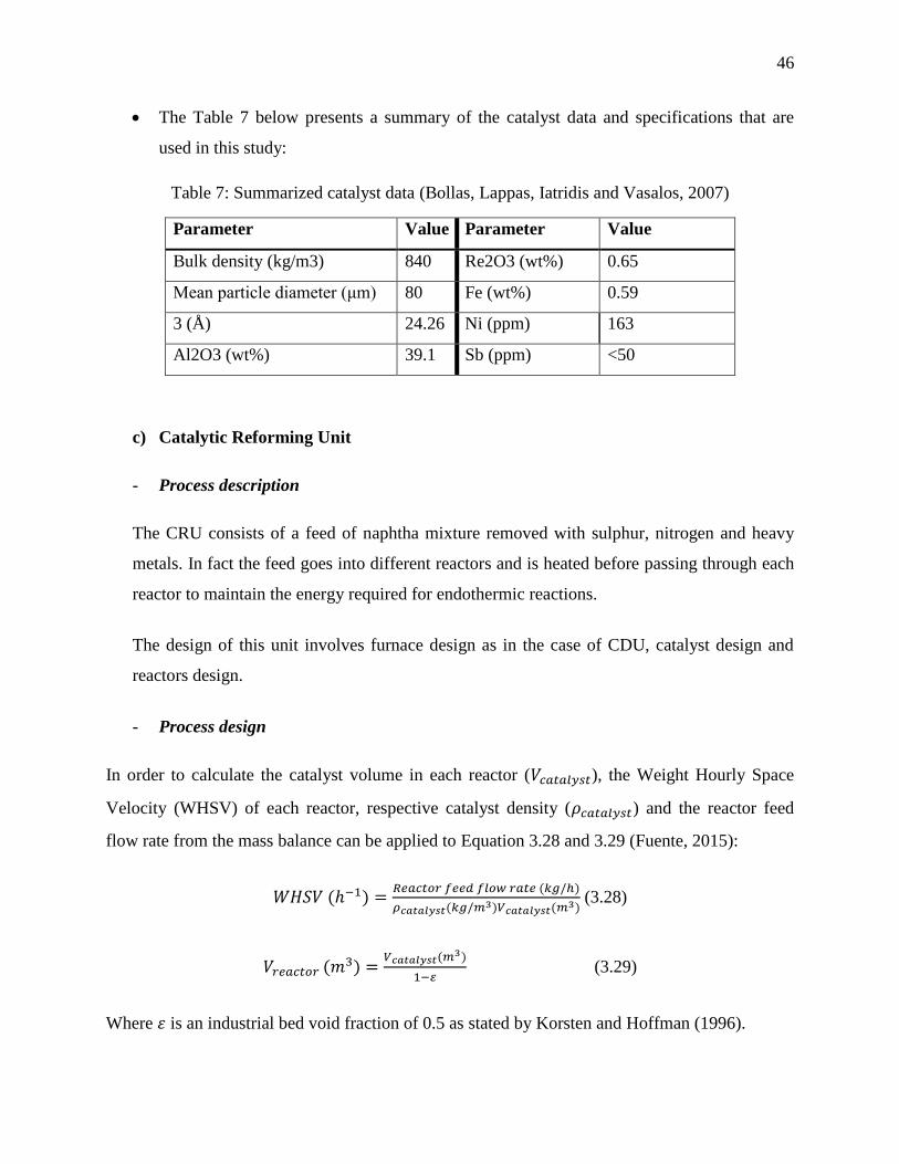
46
The Table 7 below presents a summary of the catalyst data and specifications that are
used in this study:
Table 7: Summarized catalyst data (Bollas, Lappas, Iatridis and Vasalos, 2007)
Parameter Value Parameter Value
Bulk density (kg/m3) 840 Re2O3 (wt%) 0.65
Mean particle diameter (μm) 80 Fe (wt%) 0.59
3 (Å) 24.26 Ni (ppm) 163
Al2O3 (wt%) 39.1 Sb (ppm) <50
c) Catalytic Reforming Unit
- Process description
The CRU consists of a feed of naphtha mixture removed with sulphur, nitrogen and heavy
metals. In fact the feed goes into different reactors and is heated before passing through each
reactor to maintain the energy required for endothermic reactions.
The design of this unit involves furnace design as in the case of CDU, catalyst design and
reactors design.
- Process design
In order to calculate the catalyst volume in each reactor (𝑉𝑐𝑎𝑡𝑎𝑙𝑦𝑠𝑡), the Weight Hourly Space
Velocity (WHSV) of each reactor, respective catalyst density (𝜌𝑐𝑎𝑡𝑎𝑙𝑦𝑠𝑡) and the reactor feed
flow rate from the mass balance can be applied to Equation 3.28 and 3.29 (Fuente, 2015):
𝑊𝐻𝑆𝑉 (ℎ−1) =𝑅𝑒𝑎𝑐𝑡𝑜𝑟 𝑓𝑒𝑒𝑑 𝑓𝑙𝑜𝑤 𝑟𝑎𝑡𝑒 (𝑘𝑔/ℎ)
𝜌𝑐𝑎𝑡𝑎𝑙𝑦𝑠𝑡(𝑘𝑔/𝑚3)𝑉𝑐𝑎𝑡𝑎𝑙𝑦𝑠𝑡(𝑚3) (3.28)
𝑉𝑟𝑒𝑎𝑐𝑡𝑜𝑟 (𝑚3) =𝑉𝑐𝑎𝑡𝑎𝑙𝑦𝑠𝑡(𝑚3)
1− (3.29)
Where 휀 is an industrial bed void fraction of 0.5 as stated by Korsten and Hoffman (1996).
47
d) Hydrotreatment Unit
- Process description
The feed of this unit is mixed with hydrogen gas before being fed into a furnace to increase
the temperature the range of 316 to 427oC. The mixture enters a fixed bed reactor where
sulphur and nitrogen are converted to hydrogen sulphide and ammonia. The hydrotreater
operates at pressures between 70,307 to 210,921 kg/m2 (Albahri, 2001).
- Process design
The design of the process will consist of a calculation of the catalyst volume and WHSV as
done in equation 3.28 and 3.29.
3.3. Modelling
3.3.1. Distillation
Due to the complexities of crude oil feed and petroleum products, it is essential to develop an
appropriate algorithm for the simulation of multi-component mixture separation (Douani,
Ouadjenia and Terkhi, 2007a; Sridhar and Lucia, 1990). The development and improvement of
distillation modelling have been carried out in many researches and, at the same instance, tools
such as Aspen Plus (Aspentech), PRO/II (SimSci-Esscor) and the IITM design (ChemShare),
have been developed and used for common modelling (Li et al., 2005).
Approximate, equilibrium and rate based methods are the three classes of simulation methods for
distillation columns which have been developed according to different assumptions made during
the development of models (Jelinet and Hlavecek, 1975; Gañí, R., Ruiz, C.A. and Cameron,
1986). Amongst these methods the equilibrium method, which is the most commonly used
method, develops and solves the MESH equations (Material balance equation, Equilibrium phase
equations, Summation equations and Heat balance equations) (Ramesh, et al., 2007). The model
equations that describe multi-component separation processes are non-linear and interdependent,
irrespective of the method used, and solutions are complex iterative and difficult to converge
(Abdullah et al., 2007; Boston and Sullivan, 1974; Jaroslav, Hlavacek, and Kubicek 1973;
48
Ivakpour and Kasiri, 2008). The performed matrix method was used by Rosendo (2003) and
Douani, et al. (2007) as solution of the MESH equations.
In this work, the degree of freedom analysis of distillation column will be mathematically
modelled. Steady state simulation of distillation unit is considered as well as the MESH
equations of input and output. The atmospheric distillation and the vacuum distillation are
assumed to occur in the column.
a) Data and consideration
Inspired by Akpa and Umuze (2013), and Kumar et al. (2001), considering the system showed in
the Figure 3, MESH equations for productions of Gas (i=1), Naphtha (N; i=2), Kerosene (K;
i=3), diesel (i=4), light gasoil (LG; i=5), heavy gasoil (HG; i=6) and residue (i=7) are:
Material balance (M equation):
𝐹 = ∑ 𝑆𝑡𝑟𝑒𝑎𝑚𝑗7𝑗=1 (3.30)
∑ 𝐹 𝑍𝑖7𝑖=1 = ∑ 𝑋𝑖 𝑆𝑡𝑟𝑒𝑎𝑚𝑗
77𝑖=1𝑗=1
(3.31)
Equilibrium relationships (E equation):
𝑌𝑖,𝑗 = 𝐾𝑖,𝑗𝑋𝑖,𝑗 (3.32)
Where: 1 ≤ 𝑗 ≤ 𝑁𝑡 and 1 ≤ 𝑖 ≤ 7
𝑁𝑡: Number of tray
7: Number of main constituents (cuts)
Summation of mole fraction (S equation):
𝐿𝑖 𝑓𝑒𝑒𝑑 = ∑ 𝐿𝑖7𝑖=1 (3.33)
Where: 𝐿𝑖: liquid flow from the process
𝐿𝑖 𝑓𝑒𝑒𝑑: Liquid flow into the process
Heat balance (H equation):
𝐹 ∗ ℎ𝑓 + 𝑞 = ∑ 𝑆𝑖ℎ𝑖7𝑖=1 (3.34)
Where: 𝑆𝑖: side stream
𝑞: heat flow into
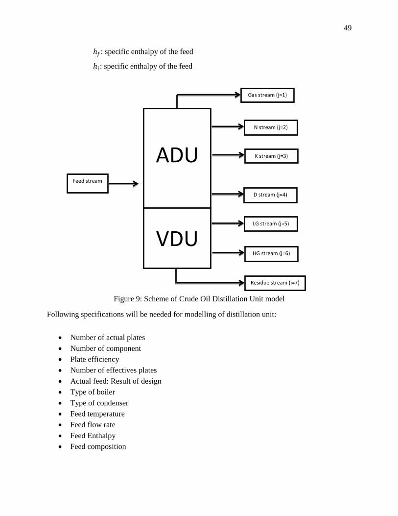
49
ℎ𝑓: specific enthalpy of the feed
ℎ𝑖: specific enthalpy of the feed
Figure 9: Scheme of Crude Oil Distillation Unit model
Following specifications will be needed for modelling of distillation unit:
Number of actual plates
Number of component
Plate efficiency
Number of effectives plates
Actual feed: Result of design
Type of boiler
Type of condenser
Feed temperature
Feed flow rate
Feed Enthalpy
Feed composition
ADU
Gas stream (j=1)
N stream (j=2)
D stream (j=4)
LG stream (j=5)
HG stream (j=6)
Residue stream (i=7)
K stream (j=3)
Feed stream
VDU
50
b) Assumptions
Here are assumptions that will be taken into account for modelling of distillation:
The column is perfectly insulated, there is no heat lost
Vapour of each tray is neglected
Process will be considering as a binary distillation where components are: Light Key (LK
which is gas) and Heavy Key (HK which is residue)
The feed is a saturated liquid
All the tray are ideal (100% of efficiency)
The molar vaporisation of LK and HK are approximately equal
Number of trays will be calculated during design of column and will exclude reboiler and
condenser.
Feed stage will be obtain by design calculation
Perfect mixing of each stage
Relative volatility of component remains constant throughout the column
Condenser and reboiler dynamics are neglected
On the basis of the first three first assumptions, we can easily conclude that the vapour coming
out of the first stage is equal to the one coming out of the second, equal to that coming out of the
third, etc. This can be written as follow:
𝑉1 = 𝑉2 = 𝑉3 = ⋯ = 𝑉𝑟𝑒𝑠𝑖𝑑𝑢𝑒 (3.35)
c) Procedure
The modelling of distillation will be taking into account 4 sections of the distillation column, as
illustrated in figure 10:
Reflux drum
Top stage (Nth
stage of distillation)
nth
stage of distillation
Feed section
First stage
Bottom stage
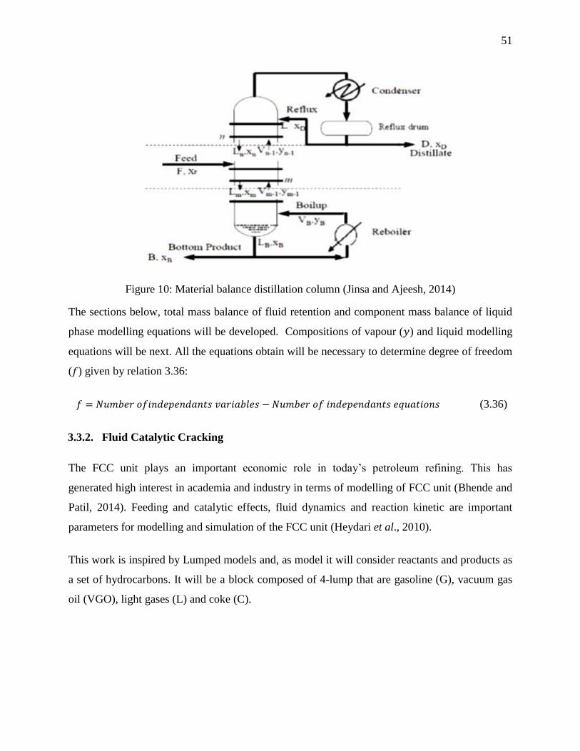
51
Figure 10: Material balance distillation column (Jinsa and Ajeesh, 2014)
The sections below, total mass balance of fluid retention and component mass balance of liquid
phase modelling equations will be developed. Compositions of vapour (𝑦) and liquid modelling
equations will be next. All the equations obtain will be necessary to determine degree of freedom
(𝑓) given by relation 3.36:
𝑓 = 𝑁𝑢𝑚𝑏𝑒𝑟 𝑜𝑓𝑖𝑛𝑑𝑒𝑝𝑒𝑛𝑑𝑎𝑛𝑡𝑠 𝑣𝑎𝑟𝑖𝑎𝑏𝑙𝑒𝑠 − 𝑁𝑢𝑚𝑏𝑒𝑟 𝑜𝑓 𝑖𝑛𝑑𝑒𝑝𝑒𝑛𝑑𝑎𝑛𝑡𝑠 𝑒𝑞𝑢𝑎𝑡𝑖𝑜𝑛𝑠 (3.36)
3.3.2. Fluid Catalytic Cracking
The FCC unit plays an important economic role in today’s petroleum refining. This has
generated high interest in academia and industry in terms of modelling of FCC unit (Bhende and
Patil, 2014). Feeding and catalytic effects, fluid dynamics and reaction kinetic are important
parameters for modelling and simulation of the FCC unit (Heydari et al., 2010).
This work is inspired by Lumped models and, as model it will consider reactants and products as
a set of hydrocarbons. It will be a block composed of 4-lump that are gasoline (G), vacuum gas
oil (VGO), light gases (L) and coke (C).
52
a) Data
Following specifications will be needed for modelling of FCC unit:
Feed
Catalyst
Catalyst to oil ratio
Weight fraction of each components involve
Ratio of molecular weight
b) Assumptions
Here are assumptions that will be taken into account for modelling of FCCU:
Isothermal condition
Constant hold-up
Constant pressure
Constant density
Feed viscosity and heat capacities of all components are constant
Perfect mixed
Unreacted gases are off the top of reactor
Vapour-phase dynamics very fast
FCC riser is a conversion reactor and FCC reactor is a continuous stirred-tank reactor
The coke deposit on the catalyst does not affect the fluid flow
All cracking reactions are considered taking place in the riser
c) Procedure
Drawing of schematic diagram representing reactions scheme, that makes the equations from the
constituted network.
53
3.3.3. Catalytic Reforming Unit
The modelling is frequently based on the type of kinetic model used and the number of reactive
species (Askari et al., 2012). This study will take account pseudo components to reduce
complications. Naphtene, aromatic and paraffins are pseudo components considered by the
Smith model and also used in this work.
Knowing that catalyst deactivation is defined as the ratio of the reaction rate at a time t and the
reaction rate at the beginning start of a cycle.
The following assumptions will be taken into account for modelling of FCCU:
Catalytic reforming proves is considered as an isothermal condition
Reactions are represented by simple first order
Based on the reactions rate equations, the modelling procedure will consist of considering an
initial rate with a certain temperature (T0) and a rate at a certain temperature (T). Then the
development will take place from there.
3.3.4. Hydrotreatment modelling
A couple of physical and chemical processes take place in a catalytic process and influence the
overall reaction rate (Rivotti, 2009). The model is then more or less detailed depending on the
number of phenomena taken into account in the process.
a) Data
Based on phenomena taking place in hydrotreatment following data were considered:
Molar concentration
Reaction rate constant
Temperature range
Pressure range
WHSV ranges
54
b) Assumptions
The following parameters are the assumptions made for modelling of hydrotreatment:
Reactions occurs in the kinetic area
The order of reactions is the first
Reactions of hydrogenolis are reaction of first order in quasi homogeneous conditions
Pseudo homogene reactions
Hydrogen is feed in excess, so its concentration is constant along the reactor
Isothermal conditions along the reactor.
c) Procedure
Comparison of different models used. Here are models considered:
Chang and Fang model
Korsten and Hoffman model
Murali and voolapali
3.4. Simulation of modular refinery
The computer simulation of this study was carried out using Aspen Hysys simulation software.
With unique characteristics among chemical processes, petroleum refining processes are
extremely complex and integrated. To manage the simulation of petroleum processes Aspen
Hysys can be used. Aspen Hysys is an advanced process simulation environment for processes
that provide special features to develop a model of petroleum process; and then use this model to
study alternative modes of operation or optimize the existing operation (AspenTech, 2009).
3.4.1. Process simulation procedure
The computer simulation was carried out according to the following procedure:
- Data collection: Refinery process and operation data were collected from literature
and Kutubu (crude assay).
- Construction of the modular refinery: Building the model of the refinery designed
using the data collected.
- Computer simulation: Carried out using Aspen Hysys
55
3.4.2. Process simulation
The computer simulation software was used to carry out complete modelling and process
simulation of the refinery in order to obtain reasonable design parameters. Reliable process
operation data such as thermodynamic packages were provided by Aspen Hysys.
Mainly, process simulation involved the following simulation:
1. Defining feedstock
2. Selecting thermodynamic package
3. Specify modular refinery capacity
4. Assigning proper operation units and settings up input operating conditions
3.5. Environmental study
This section explains how the environmental results obtained were analysed as the study focused
on the environmental impact of the fuels produced by a modular refinery.
The environmental study of this research is a combination of exploratory and experimental
survey. The exploratory part is the research for studies related to environmental impact of
refinery products; and experimental part being mainly based on the simulation of the designed
modular refinery. According to Saunders et al. (2009), documentary data include written
materials such as notices, correspondence (including emails), meeting minutes, annual
sustainability reports, diaries, speech transcripts and administrative and public records. In our
case, the document search process has taken following steps:
- Search for relevant keywords in databases (keyword was use to limit the search results);
- Search the databases again with the new references as keywords or relative information;
- Collect the most relevant argument and data from the search results, and make the
comments on the information obtained.
The research process took place with the usage of the Internet by downloading documents or
reports with environmental impacts as output from the refinery and by categorising the extracted
literature (process or product pollution).
56
The reports and studies or research constituting documentary data are the following:
- Buckle et al (2008): This study showed that a modular refinery could be considered as a
new and better technology, based on environmental, social and economic considerations
stipulated by the United Nation framework Consideration on climate Change (UNFCC)
in 1992.
- Adefarati and Chigbu (2017): This research concluded that the modular refinery would
lead to an overall reduction in pollutants emissions. This will have an impact on the
production of the conventional refineries by increasing the capacity. Most importantly, it
would serve as a climate mitigating tool.
- Muhsin et al (2016): The optimisation of the crude oil hydrotreatment unit in this study
was carried out in order to maximise sulphur removal in the product. Usage of Bootstrap
aggregated neural network for modelling and optimising the process based on results
such as the existence of a trace-off between sulphur removal and the production rate (for
instance 40.00 m3/h, which is the smallest feed makes the highest sulphur removal of
95.82%).
- Sharma (2018): This study used laboratory-scale reactor and industrial data to achieve
its goal. Based on the development of the Graphical User Interface (GUI) to compare the
sulphur concentration measured in the product and the expected sulphur concentration
predicted.
- Shokri et al (2007): the results of this research have shown that the sulphur content
decrease as the temperature increases while the pressure and 𝐻2/𝑜𝑖𝑙 ratio are constant. It
has been observed that by increasing 𝐻2/oil ratio to 55.7, the sulphur concentration
decreases, but it increases again by increasing 𝐻2/𝑜𝑖𝑙. 55.7 was then the optimal 𝐻2/𝑜𝑖𝑙
ratio.
- Al-Malki (2004): based on the use of the oxidation extraction technique for the reduction
of sulphur in gasoline and diesel, this study showed that the technique is promising for
the reduction of sulphur below of 100 ppm from the value of 1044 ppm with a total
removal of 92%.
- Abubakar et al (2016): the study aims to reduce the sulphur content in crude oil from the
Urals using oxidative desulphurization. The results obtained have shown that the
57
reduction in the sulphur content of refinery products increase with the increase in amount
of oxidant. In fact, the content of gasoline, kerosene, diesel and residue sulphur were
reduced respectively from 0.0805 to 0.0548 wt%, from 0.2086 to 0.1150 wt%, from
0.7754 to 0.2698 wt% and from 1.6426 wt% to 0.4110 wt%.
- Gupta (2006): the study concluded that gasoline yield increases with the increase in
COR; however, the rate of increase in the gasoline yield decreases at higher COR values.
- Paul et al (2015): the researchers built a model to predict the conversion of feed oil and
formation of gasoline. The results showed that when the COR is 4.5, the gasoline yield is
55.89. When the COR goes to 8.5, the yield is 58.9%.
Richmond (2006) defined qualitative data as data represented in verbal or narrative form, and
qualitative data as data expressed in numerical terms in which the numerical values could be
large or small. Knowing that the data provided by the Aspen simulation are numerical and can be
represented in table or a curve, the results of our research will certainly be quantitative.
Qualitative data obtain from literature are also used for assessment.
The scope of the environmental study will be limited to the use of the software to illustrate
production of the modular refinery. A simulation with the use of ASPEN HYSYS was performed
out in order to generate enough data for the analysis. Data analyses were obtained from the
simulation results.
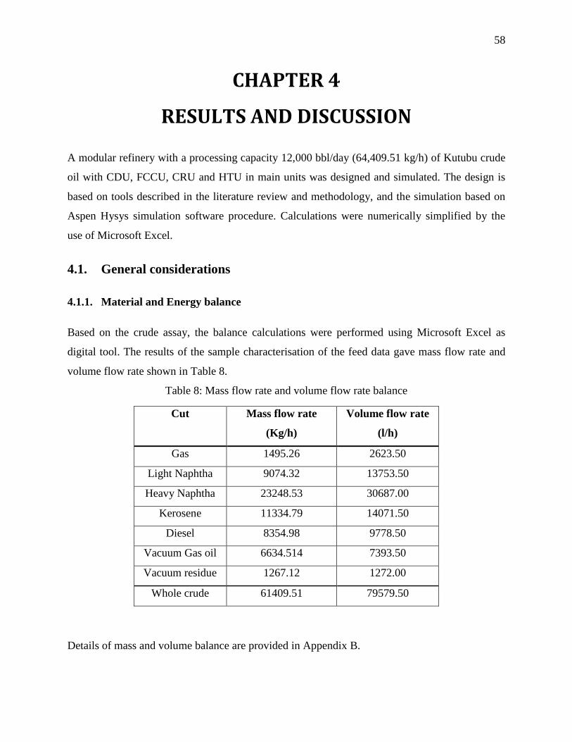
58
CHAPTER 4
RESULTS AND DISCUSSION
A modular refinery with a processing capacity 12,000 bbl/day (64,409.51 kg/h) of Kutubu crude
oil with CDU, FCCU, CRU and HTU in main units was designed and simulated. The design is
based on tools described in the literature review and methodology, and the simulation based on
Aspen Hysys simulation software procedure. Calculations were numerically simplified by the
use of Microsoft Excel.
4.1. General considerations
4.1.1. Material and Energy balance
Based on the crude assay, the balance calculations were performed using Microsoft Excel as
digital tool. The results of the sample characterisation of the feed data gave mass flow rate and
volume flow rate shown in Table 8.
Table 8: Mass flow rate and volume flow rate balance
Cut Mass flow rate
(Kg/h)
Volume flow rate
(l/h)
Gas 1495.26 2623.50
Light Naphtha 9074.32 13753.50
Heavy Naphtha 23248.53 30687.00
Kerosene 11334.79 14071.50
Diesel 8354.98 9778.50
Vacuum Gas oil 6634.514 7393.50
Vacuum residue 1267.12 1272.00
Whole crude 61409.51 79579.50
Details of mass and volume balance are provided in Appendix B.
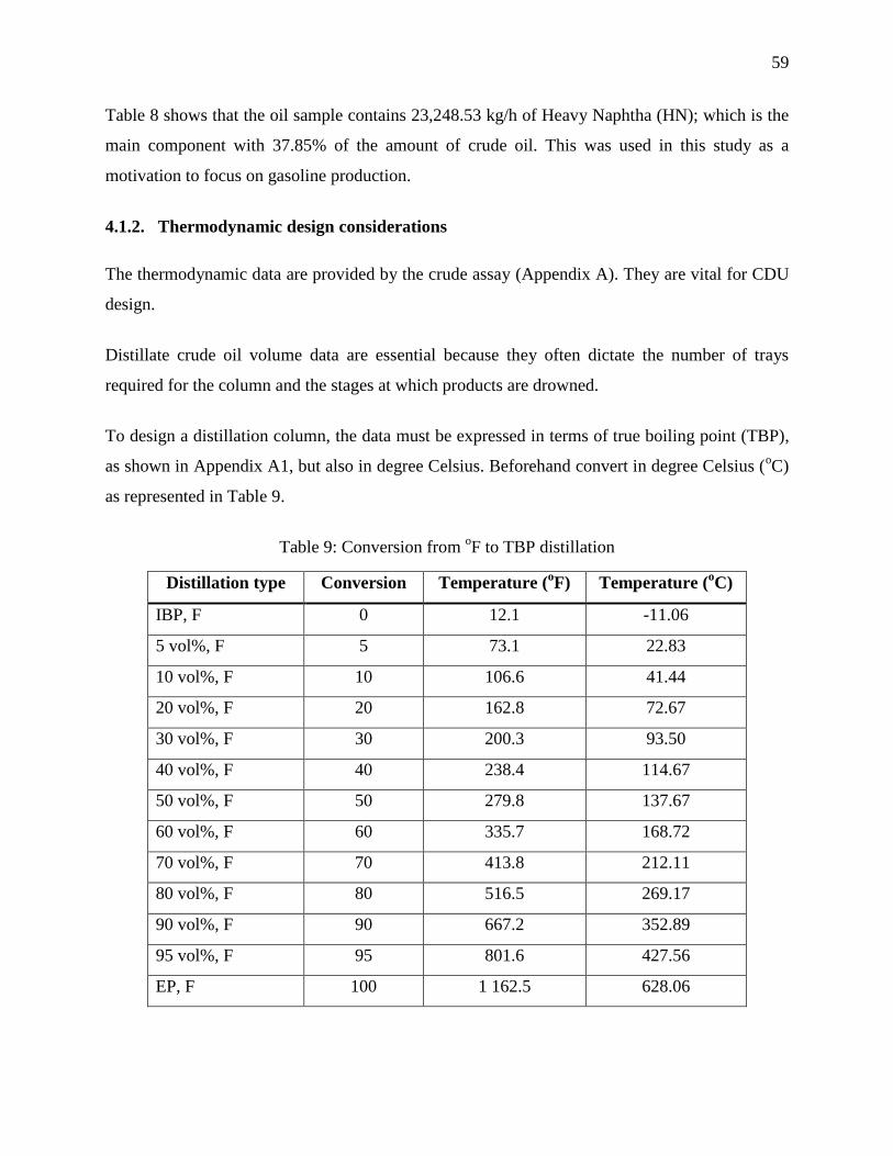
59
Table 8 shows that the oil sample contains 23,248.53 kg/h of Heavy Naphtha (HN); which is the
main component with 37.85% of the amount of crude oil. This was used in this study as a
motivation to focus on gasoline production.
4.1.2. Thermodynamic design considerations
The thermodynamic data are provided by the crude assay (Appendix A). They are vital for CDU
design.
Distillate crude oil volume data are essential because they often dictate the number of trays
required for the column and the stages at which products are drowned.
To design a distillation column, the data must be expressed in terms of true boiling point (TBP),
as shown in Appendix A1, but also in degree Celsius. Beforehand convert in degree Celsius (oC)
as represented in Table 9.
Table 9: Conversion from oF to TBP distillation
Distillation type Conversion Temperature (oF) Temperature (
oC)
IBP, F 0 12.1 -11.06
5 vol%, F 5 73.1 22.83
10 vol%, F 10 106.6 41.44
20 vol%, F 20 162.8 72.67
30 vol%, F 30 200.3 93.50
40 vol%, F 40 238.4 114.67
50 vol%, F 50 279.8 137.67
60 vol%, F 60 335.7 168.72
70 vol%, F 70 413.8 212.11
80 vol%, F 80 516.5 269.17
90 vol%, F 90 667.2 352.89
95 vol%, F 95 801.6 427.56
EP, F 100 1 162.5 628.06
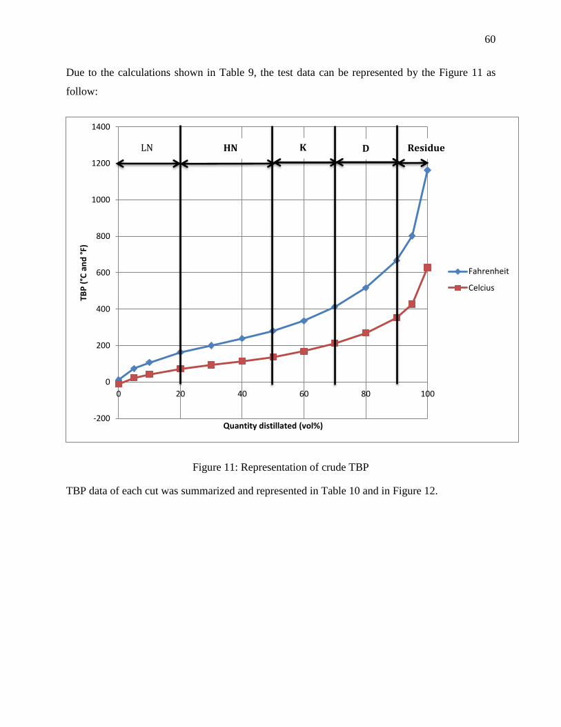
60
Due to the calculations shown in Table 9, the test data can be represented by the Figure 11 as
follow:
Figure 11: Representation of crude TBP
TBP data of each cut was summarized and represented in Table 10 and in Figure 12.
-200
0
200
400
600
800
1000
1200
1400
0 20 40 60 80 100
TBP
(°C
an
d °
F)
Quantity distillated (vol%)
Fahrenheit
Celcius
LN HN K D Residue
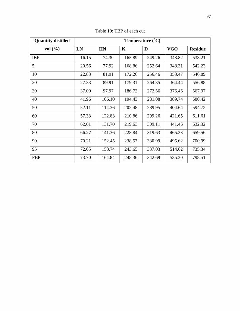
61
Table 10: TBP of each cut
Quantity distilled
vol (%)
Temperature (oC)
LN HN K D VGO Residue
IBP 16.15 74.30 165.89 249.26 343.82 538.21
5 20.56 77.92 168.86 252.64 348.31 542.23
10 22.83 81.91 172.26 256.46 353.47 546.89
20 27.33 89.91 179.31 264.35 364.44 556.88
30 37.00 97.97 186.72 272.56 376.46 567.97
40 41.96 106.10 194.43 281.08 389.74 580.42
50 52.11 114.36 202.48 289.95 404.64 594.72
60 57.33 122.83 210.86 299.26 421.65 611.61
70 62.01 131.70 219.63 309.11 441.46 632.32
80 66.27 141.36 228.84 319.63 465.33 659.56
90 70.21 152.45 238.57 330.99 495.62 700.99
95 72.05 158.74 243.65 337.03 514.62 735.34
FBP 73.70 164.84 248.36 342.69 535.20 798.51
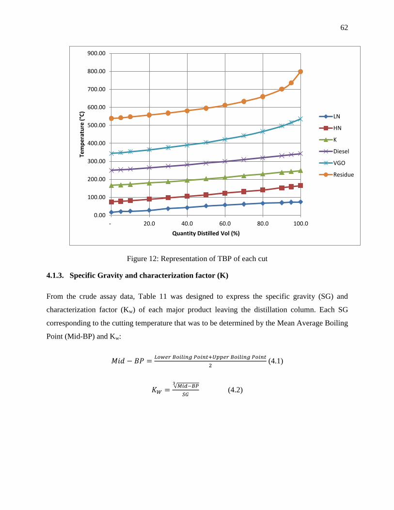
62
Figure 12: Representation of TBP of each cut
4.1.3. Specific Gravity and characterization factor (K)
From the crude assay data, Table 11 was designed to express the specific gravity (SG) and
characterization factor (Kw) of each major product leaving the distillation column. Each SG
corresponding to the cutting temperature that was to be determined by the Mean Average Boiling
Point (Mid-BP) and Kw:
𝑀𝑖𝑑 − 𝐵𝑃 =𝐿𝑜𝑤𝑒𝑟 𝐵𝑜𝑖𝑙𝑖𝑛𝑔 𝑃𝑜𝑖𝑛𝑡+𝑈𝑝𝑝𝑒𝑟 𝐵𝑜𝑖𝑙𝑖𝑛𝑔 𝑃𝑜𝑖𝑛𝑡
2 (4.1)
𝐾𝑊 =√𝑀𝑖𝑑−𝐵𝑃
3
𝑆𝐺 (4.2)
0.00
100.00
200.00
300.00
400.00
500.00
600.00
700.00
800.00
900.00
- 20.0 40.0 60.0 80.0 100.0
Tem
pe
ratu
re (°C
)
Quantity Distilled Vol (%)
LN
HN
K
Diesel
VGO
Residue
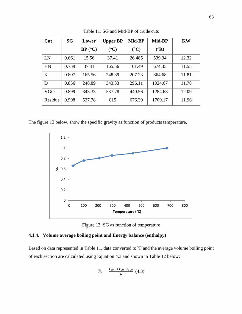
63
Table 11: SG and Mid-BP of crude cuts
Cut SG Lower
BP (°C)
Upper BP
(°C)
Mid-BP
(°C)
Mid-BP
(°R)
KW
LN 0.661 15.56 37.41 26.485 539.34 12.32
HN 0.759 37.41 165.56 101.49 674.35 11.55
K 0.807 165.56 248.89 207.23 864.68 11.81
D 0.856 248.89 343.33 296.11 1024.67 11.78
VGO 0.899 343.33 537.78 440.56 1284.68 12.09
Residue 0.998 537.78 815 676.39 1709.17 11.96
The figure 13 below, show the specific gravity as function of products temperature.
Figure 13: SG as function of temperature
4.1.4. Volume average boiling point and Energy balance (enthalpy)
Based on data represented in Table 11, data converted to oF and the average volume boiling point
of each section are calculated using Equation 4.3 and shown in Table 12 below:
𝑇𝑉 =𝑡10+4 𝑡50+𝑡100
6 (4.3)
0
0.2
0.4
0.6
0.8
1
1.2
0 100 200 300 400 500 600 700 800
SG
Temperature (°C)
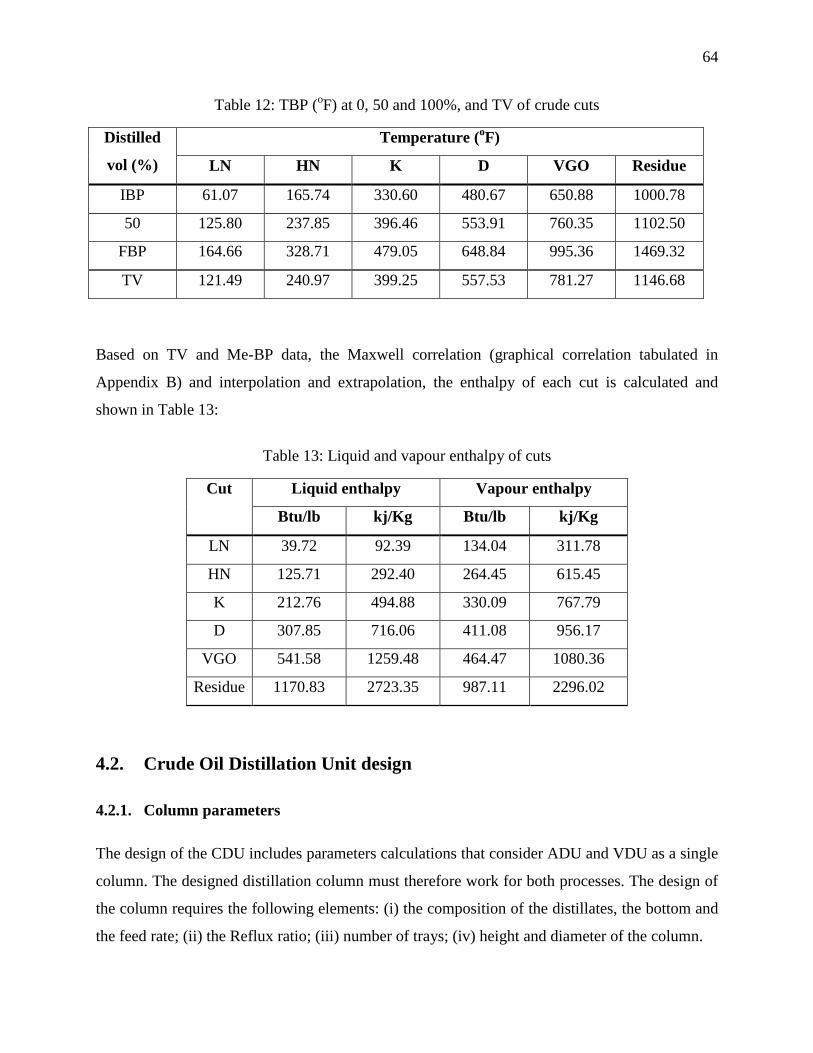
64
Table 12: TBP (oF) at 0, 50 and 100%, and TV of crude cuts
Distilled
vol (%)
Temperature (oF)
LN HN K D VGO Residue
IBP 61.07 165.74 330.60 480.67 650.88 1000.78
50 125.80 237.85 396.46 553.91 760.35 1102.50
FBP 164.66 328.71 479.05 648.84 995.36 1469.32
TV 121.49 240.97 399.25 557.53 781.27 1146.68
Based on TV and Me-BP data, the Maxwell correlation (graphical correlation tabulated in
Appendix B) and interpolation and extrapolation, the enthalpy of each cut is calculated and
shown in Table 13:
Table 13: Liquid and vapour enthalpy of cuts
Cut Liquid enthalpy Vapour enthalpy
Btu/lb kj/Kg Btu/lb kj/Kg
LN 39.72 92.39 134.04 311.78
HN 125.71 292.40 264.45 615.45
K 212.76 494.88 330.09 767.79
D 307.85 716.06 411.08 956.17
VGO 541.58 1259.48 464.47 1080.36
Residue 1170.83 2723.35 987.11 2296.02
4.2. Crude Oil Distillation Unit design
4.2.1. Column parameters
The design of the CDU includes parameters calculations that consider ADU and VDU as a single
column. The designed distillation column must therefore work for both processes. The design of
the column requires the following elements: (i) the composition of the distillates, the bottom and
the feed rate; (ii) the Reflux ratio; (iii) number of trays; (iv) height and diameter of the column.
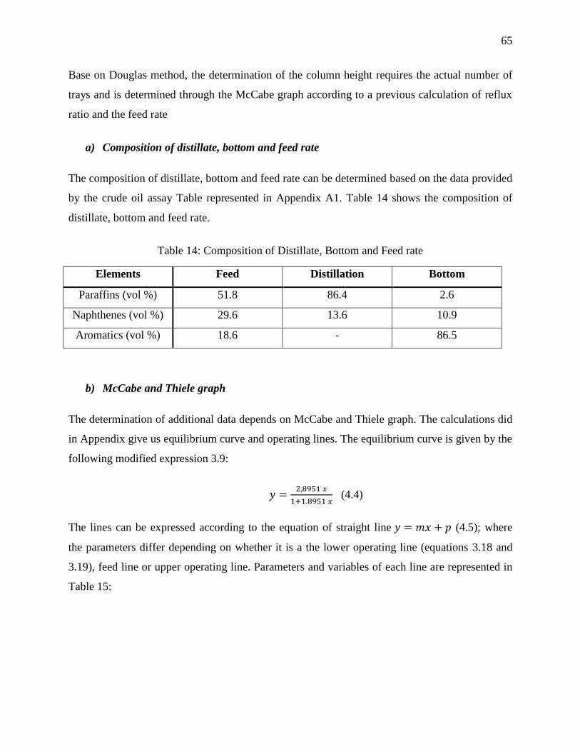
65
Base on Douglas method, the determination of the column height requires the actual number of
trays and is determined through the McCabe graph according to a previous calculation of reflux
ratio and the feed rate
a) Composition of distillate, bottom and feed rate
The composition of distillate, bottom and feed rate can be determined based on the data provided
by the crude oil assay Table represented in Appendix A1. Table 14 shows the composition of
distillate, bottom and feed rate.
Table 14: Composition of Distillate, Bottom and Feed rate
Elements Feed Distillation Bottom
Paraffins (vol %) 51.8 86.4 2.6
Naphthenes (vol %) 29.6 13.6 10.9
Aromatics (vol %) 18.6 - 86.5
b) McCabe and Thiele graph
The determination of additional data depends on McCabe and Thiele graph. The calculations did
in Appendix give us equilibrium curve and operating lines. The equilibrium curve is given by the
following modified expression 3.9:
𝑦 =2,8951 𝑥
1+1.8951 𝑥 (4.4)
The lines can be expressed according to the equation of straight line 𝑦 = 𝑚𝑥 + 𝑝 (4.5); where
the parameters differ depending on whether it is a the lower operating line (equations 3.18 and
3.19), feed line or upper operating line. Parameters and variables of each line are represented in
Table 15:
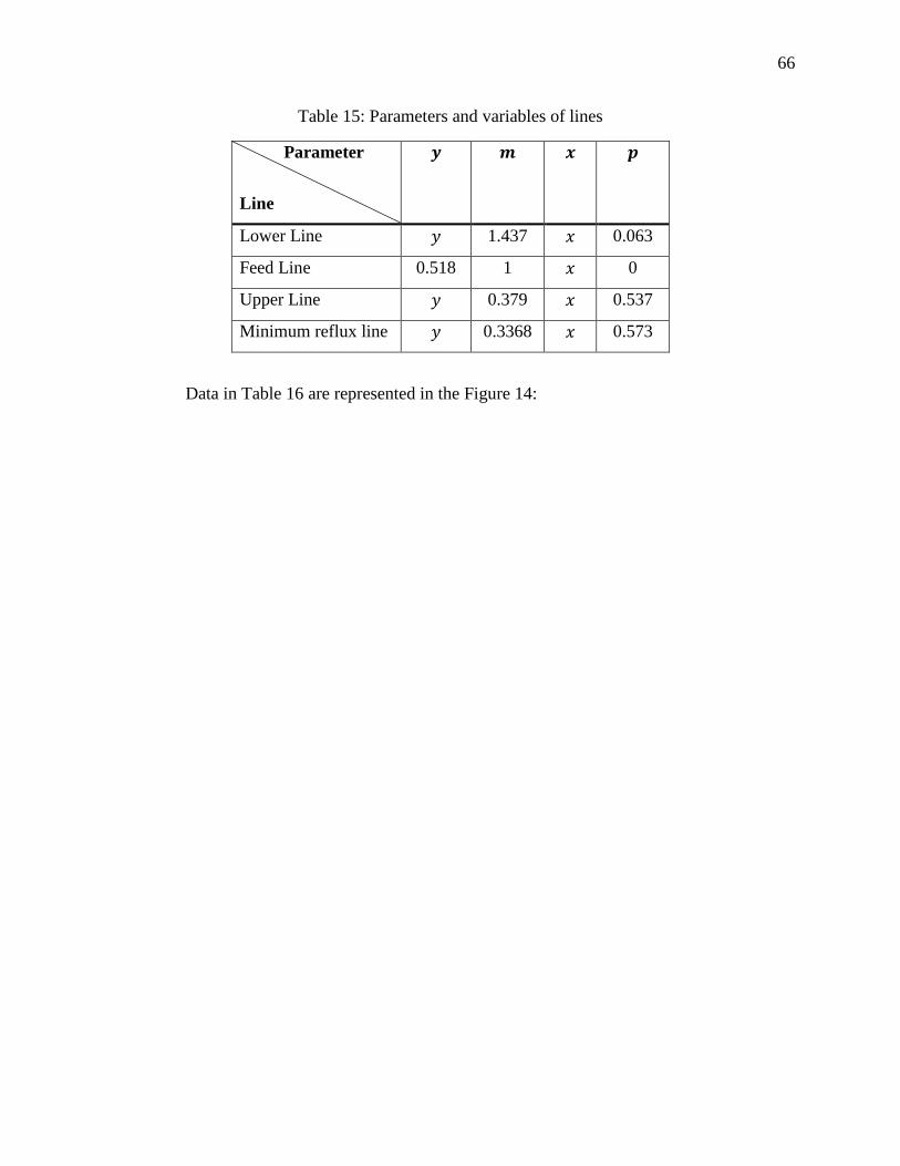
66
Table 15: Parameters and variables of lines
Parameter
Line
𝒚 𝒎 𝒙 𝒑
Lower Line 𝑦 1.437 𝑥 0.063
Feed Line 0.518 1 𝑥 0
Upper Line 𝑦 0.379 𝑥 0.537
Minimum reflux line 𝑦 0.3368 𝑥 0.573
Data in Table 16 are represented in the Figure 14:
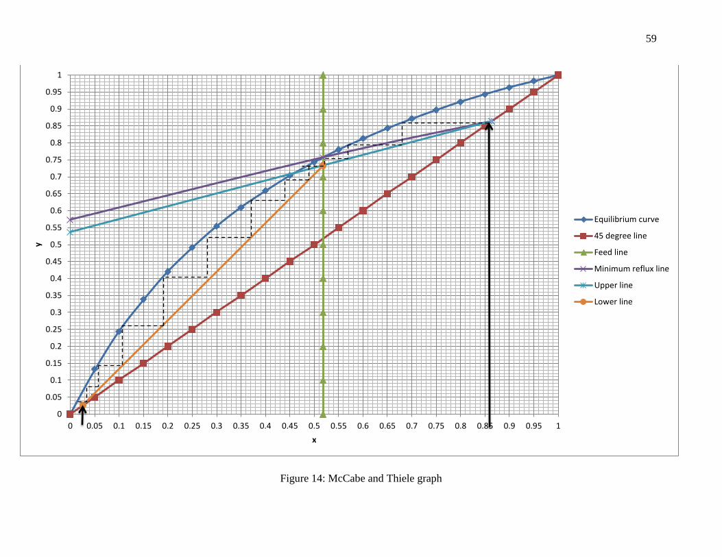
59
Figure 14: McCabe and Thiele graph
0
0.05
0.1
0.15
0.2
0.25
0.3
0.35
0.4
0.45
0.5
0.55
0.6
0.65
0.7
0.75
0.8
0.85
0.9
0.95
1
0 0.05 0.1 0.15 0.2 0.25 0.3 0.35 0.4 0.45 0.5 0.55 0.6 0.65 0.7 0.75 0.8 0.85 0.9 0.95 1
y
x
Equilibrium curve
45 degree line
Feed line
Minimum reflux line
Upper line
Lower line
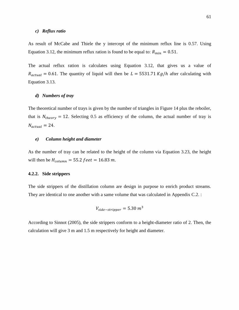
61
c) Reflux ratio
As result of McCabe and Thiele the y intercept of the minimum reflux line is 0.57. Using
Equation 3.12, the minimum reflux ration is found to be equal to: 𝑅𝑚𝑖𝑛 = 0.51.
The actual reflux ration is calculates using Equation 3.12, that gives us a value of
𝑅𝑎𝑐𝑡𝑢𝑎𝑙 = 0.61. The quantity of liquid will then be 𝐿 = 5531.71 𝐾𝑔/ℎ after calculating with
Equation 3.13.
d) Numbers of tray
The theoretical number of trays is given by the number of triangles in Figure 14 plus the reboiler,
that is 𝑁𝑡ℎ𝑒𝑜𝑟𝑦 = 12. Selecting 0.5 as efficiency of the column, the actual number of tray is
𝑁𝑎𝑐𝑡𝑢𝑎𝑙 = 24.
e) Column height and diameter
As the number of tray can be related to the height of the column via Equation 3.23, the height
will then be 𝐻𝑐𝑜𝑙𝑢𝑚𝑛 = 55.2 𝑓𝑒𝑒𝑡 = 16.83 𝑚.
4.2.2. Side strippers
The side strippers of the distillation column are design in purpose to enrich product streams.
They are identical to one another with a same volume that was calculated in Appendix C.2. :
𝑉𝑠𝑖𝑑𝑒−𝑠𝑡𝑟𝑖𝑝𝑝𝑒𝑟 = 5.30 𝑚3
According to Sinnot (2005), the side strippers conform to a height-diameter ratio of 2. Then, the
calculation will give 3 m and 1.5 m respectively for height and diameter.
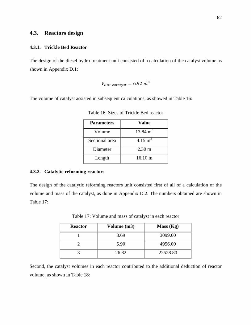
62
4.3. Reactors design
4.3.1. Trickle Bed Reactor
The design of the diesel hydro treatment unit consisted of a calculation of the catalyst volume as
shown in Appendix D.1:
𝑉𝐻𝐷𝑇 𝑐𝑎𝑡𝑎𝑙𝑦𝑠𝑡 = 6.92 𝑚3
The volume of catalyst assisted in subsequent calculations, as showed in Table 16:
Table 16: Sizes of Trickle Bed reactor
Parameters Value
Volume 13.84 m3
Sectional area 4.15 m2
Diameter 2.30 m
Length 16.10 m
4.3.2. Catalytic reforming reactors
The design of the catalytic reforming reactors unit consisted first of all of a calculation of the
volume and mass of the catalyst, as done in Appendix D.2. The numbers obtained are shown in
Table 17:
Table 17: Volume and mass of catalyst in each reactor
Reactor Volume (m3) Mass (Kg)
1 3.69 3099.60
2 5.90 4956.00
3 26.82 22528.80
Second, the catalyst volumes in each reactor contributed to the additional deduction of reactor
volume, as shown in Table 18:
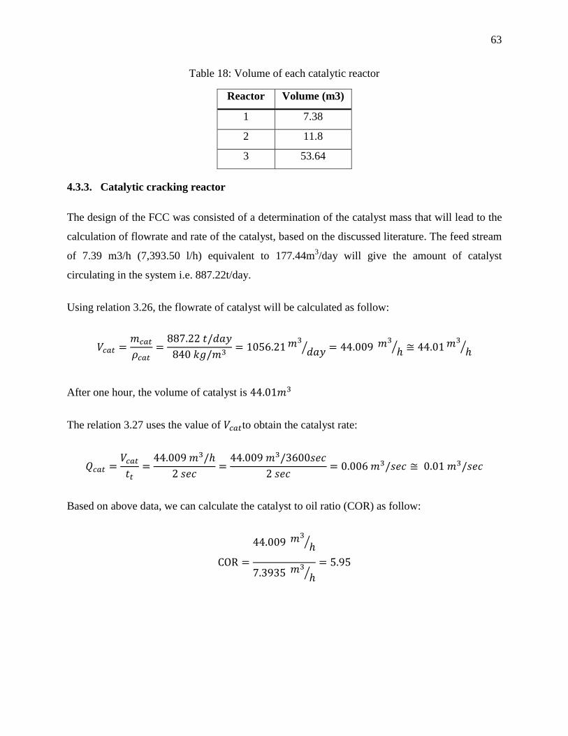
63
Table 18: Volume of each catalytic reactor
Reactor Volume (m3)
1 7.38
2 11.8
3 53.64
4.3.3. Catalytic cracking reactor
The design of the FCC was consisted of a determination of the catalyst mass that will lead to the
calculation of flowrate and rate of the catalyst, based on the discussed literature. The feed stream
of 7.39 m3/h (7,393.50 l/h) equivalent to 177.44m3/day will give the amount of catalyst
circulating in the system i.e. 887.22t/day.
Using relation 3.26, the flowrate of catalyst will be calculated as follow:
𝑉𝑐𝑎𝑡 =𝑚𝑐𝑎𝑡
𝜌𝑐𝑎𝑡=
887.22 𝑡/𝑑𝑎𝑦
840 𝑘𝑔/𝑚3= 1056.21 𝑚3
𝑑𝑎𝑦⁄ = 44.009 𝑚3
ℎ⁄ ≅ 44.01 𝑚3
ℎ⁄
After one hour, the volume of catalyst is 44.01𝑚3
The relation 3.27 uses the value of 𝑉𝑐𝑎𝑡to obtain the catalyst rate:
𝑄𝑐𝑎𝑡 =𝑉𝑐𝑎𝑡
𝑡𝑡=
44.009 𝑚3/ℎ
2 𝑠𝑒𝑐=
44.009 𝑚3/3600𝑠𝑒𝑐
2 𝑠𝑒𝑐= 0.006 𝑚3/𝑠𝑒𝑐 ≅ 0.01 𝑚3/𝑠𝑒𝑐
Based on above data, we can calculate the catalyst to oil ratio (COR) as follow:
COR =
44.009 𝑚3
ℎ⁄
7.3935 𝑚3
ℎ⁄= 5.95
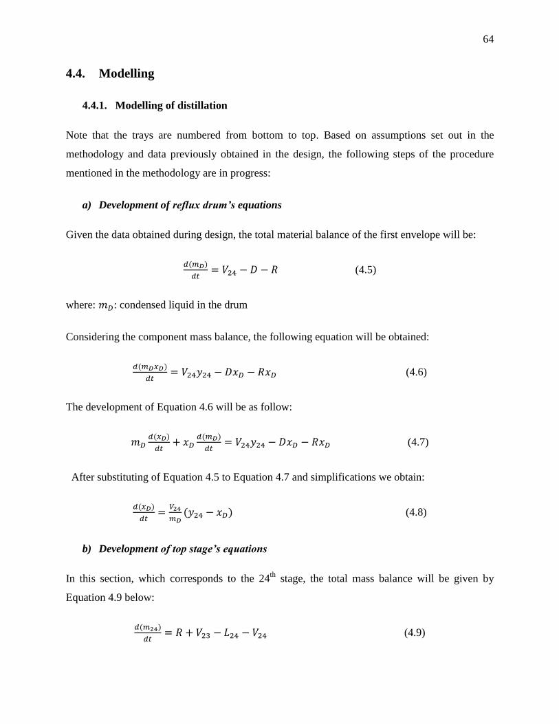
64
4.4. Modelling
4.4.1. Modelling of distillation
Note that the trays are numbered from bottom to top. Based on assumptions set out in the
methodology and data previously obtained in the design, the following steps of the procedure
mentioned in the methodology are in progress:
a) Development of reflux drum’s equations
Given the data obtained during design, the total material balance of the first envelope will be:
𝑑(𝑚𝐷)
𝑑𝑡= 𝑉24 − 𝐷 − 𝑅 (4.5)
where: 𝑚𝐷: condensed liquid in the drum
Considering the component mass balance, the following equation will be obtained:
𝑑(𝑚𝐷𝑥𝐷)
𝑑𝑡= 𝑉24𝑦24 − 𝐷𝑥𝐷 − 𝑅𝑥𝐷 (4.6)
The development of Equation 4.6 will be as follow:
𝑚𝐷𝑑(𝑥𝐷)
𝑑𝑡+ 𝑥𝐷
𝑑(𝑚𝐷)
𝑑𝑡= 𝑉24𝑦24 − 𝐷𝑥𝐷 − 𝑅𝑥𝐷 (4.7)
After substituting of Equation 4.5 to Equation 4.7 and simplifications we obtain:
𝑑(𝑥𝐷)
𝑑𝑡=
𝑉24
𝑚𝐷(𝑦24 − 𝑥𝐷) (4.8)
b) Development of top stage’s equations
In this section, which corresponds to the 24th
stage, the total mass balance will be given by
Equation 4.9 below:
𝑑(𝑚24)
𝑑𝑡= 𝑅 + 𝑉23 − 𝐿24 − 𝑉24 (4.9)
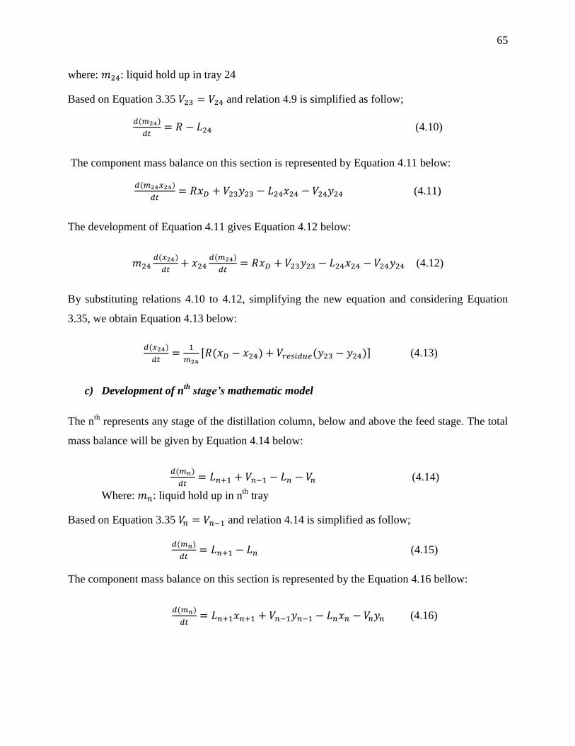
65
where: 𝑚24: liquid hold up in tray 24
Based on Equation 3.35 𝑉23 = 𝑉24 and relation 4.9 is simplified as follow;
𝑑(𝑚24)
𝑑𝑡= 𝑅 − 𝐿24 (4.10)
The component mass balance on this section is represented by Equation 4.11 below:
𝑑(𝑚24𝑥24)
𝑑𝑡= 𝑅𝑥𝐷 + 𝑉23𝑦23 − 𝐿24𝑥24 − 𝑉24𝑦24 (4.11)
The development of Equation 4.11 gives Equation 4.12 below:
𝑚24𝑑(𝑥24)
𝑑𝑡+ 𝑥24
𝑑(𝑚24)
𝑑𝑡= 𝑅𝑥𝐷 + 𝑉23𝑦23 − 𝐿24𝑥24 − 𝑉24𝑦24 (4.12)
By substituting relations 4.10 to 4.12, simplifying the new equation and considering Equation
3.35, we obtain Equation 4.13 below:
𝑑(𝑥24)
𝑑𝑡=
1
𝑚24[𝑅(𝑥𝐷 − 𝑥24) + 𝑉𝑟𝑒𝑠𝑖𝑑𝑢𝑒(𝑦23 − 𝑦24)] (4.13)
c) Development of nth
stage’s mathematic model
The nth
represents any stage of the distillation column, below and above the feed stage. The total
mass balance will be given by Equation 4.14 below:
𝑑(𝑚𝑛)
𝑑𝑡= 𝐿𝑛+1 + 𝑉𝑛−1 − 𝐿𝑛 − 𝑉𝑛 (4.14)
Where: 𝑚𝑛: liquid hold up in nth
tray
Based on Equation 3.35 𝑉𝑛 = 𝑉𝑛−1 and relation 4.14 is simplified as follow;
𝑑(𝑚𝑛)
𝑑𝑡= 𝐿𝑛+1 − 𝐿𝑛 (4.15)
The component mass balance on this section is represented by the Equation 4.16 bellow:
𝑑(𝑚𝑛)
𝑑𝑡= 𝐿𝑛+1𝑥𝑛+1 + 𝑉𝑛−1𝑦𝑛−1 − 𝐿𝑛𝑥𝑛 − 𝑉𝑛𝑦𝑛 (4.16)
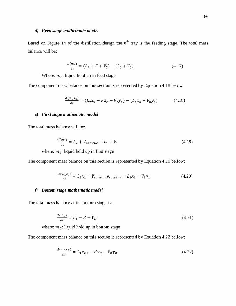
66
d) Feed stage mathematic model
Based on Figure 14 of the distillation design the 8th
tray is the feeding stage. The total mass
balance will be:
𝑑(𝑚8)
𝑑𝑡= (𝐿9 + 𝐹 + 𝑉7) − (𝐿8 + 𝑉8) (4.17)
Where: 𝑚8: liquid hold up in feed stage
The component mass balance on this section is represented by Equation 4.18 below:
𝑑(𝑚8𝑥8)
𝑑𝑡= (𝐿9𝑥9 + 𝐹𝑧𝐹 + 𝑉7𝑦8) − (𝐿8𝑥8 + 𝑉8𝑦8) (4.18)
e) First stage mathematic model
The total mass balance will be:
𝑑(𝑚1)
𝑑𝑡= 𝐿2 + 𝑉𝑟𝑒𝑠𝑖𝑑𝑢𝑒 − 𝐿1 − 𝑉1 (4.19)
where: 𝑚1: liquid hold up in first stage
The component mass balance on this section is represented by Equation 4.20 bellow:
𝑑(𝑚1𝑥1)
𝑑𝑡= 𝐿2𝑥1 + 𝑉𝑟𝑒𝑠𝑖𝑑𝑢𝑒𝑦𝑟𝑒𝑠𝑖𝑑𝑢𝑒 − 𝐿1𝑥1 − 𝑉1𝑦1 (4.20)
f) Bottom stage mathematic model
The total mass balance at the bottom stage is:
𝑑(𝑚𝐵)
𝑑𝑡= 𝐿1 − 𝐵 − 𝑉𝐵 (4.21)
where: 𝑚𝐵: liquid hold up in bottom stage
The component mass balance on this section is represented by Equation 4.22 bellow:
𝑑(𝑚𝐵𝑥𝐵)
𝑑𝑡= 𝐿1𝑥𝐵1 − 𝐵𝑥𝐵 − 𝑉𝐵𝑦𝐵 (4.22)
67
g) Determination of y and L
Knowing the relative volatility from the distillation design and based on the assumptions used, y
will be determined using equilibrium relationship (Equation 4.4).
𝑦 =2.895179 𝑥
1+(2.895179−1) 𝑥 (4.23)
The liquid flow rate is calculated using the linearized form of Francis Weir equation (hydraulic
relation):
𝐿𝑛 = 𝐿𝑛0+
𝑚𝑛−𝑚𝑛0
𝛽 (4.24)
where: 𝐿𝑛: Flow rate leaving the nth
tray of the column
𝐿𝑛0: Reference value of 𝐿𝑛
𝑚𝑛: liquid hold up in nth
tray
𝑚𝑛0: Reference value of 𝑚𝑛
𝛽: Hydraulic time constant (3 to 6 seconds per tray)
h) Degrees of freedom
First, we will determine the number of independents equations using Table 19 below:
Table 19: Independents equations
Name Number of equations
Equilibrium equation 25
Hydraulic relationship 24
Total and composition mass balance
equations
48
Reflux drum 2
Bottom column 2
Total 101
68
Similarly, the variables with corresponding number of equations are found in Table 20:
Table 20: Independent variables
Name Number of equations
Liquid composition 26
Vapour composition 25
Liquid hold up 26
Liquid flow rate 24
Feed flow rate, feed composition,
distillate flow rate, reflux, bottom
vapour, flow rate, bottom
6
Total 107
Therefore, the degree of freedom will be given by the difference between the number of
independent equations and independents variables as follow:
𝑓 = 107 − 101 = 6
Since the number of variables is greater than the number of equations, we have an underspecified
process. As this process must be specified, we must make 𝑓 equal to zero, it means:
Specification of more number of disturbance variables
This can take place by measuring following variables: Feed flow rate, feed composition
Incorporation of more number of controller equations
We can consider the bottom product (𝑥𝐵 and 𝑚𝐵) and the top product (𝑥𝐷 and 𝑚𝐷) as
controlled variables. These variables can be used to manipulate 𝑚𝐵, B, R and D
respectively using the following controller equations:
𝑅 = 𝑅𝑠 + 𝑘𝐶𝑅(𝑥𝐷𝑆𝑃 − 𝑥𝐷) (4.25)
𝐷 = 𝐷𝑠 + 𝑘𝐶𝐷(𝑚𝐷𝑆𝑃 − 𝑚𝐷) (4.26)
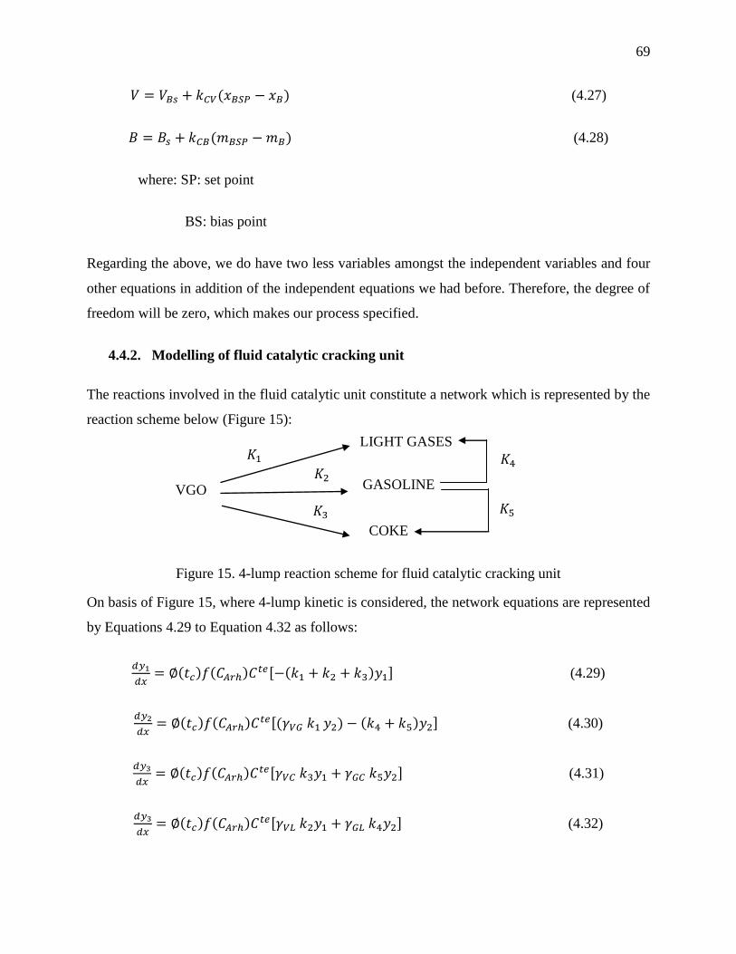
69
𝑉 = 𝑉𝐵𝑠 + 𝑘𝐶𝑉(𝑥𝐵𝑆𝑃 − 𝑥𝐵) (4.27)
𝐵 = 𝐵𝑠 + 𝑘𝐶𝐵(𝑚𝐵𝑆𝑃 − 𝑚𝐵) (4.28)
where: SP: set point
BS: bias point
Regarding the above, we do have two less variables amongst the independent variables and four
other equations in addition of the independent equations we had before. Therefore, the degree of
freedom will be zero, which makes our process specified.
4.4.2. Modelling of fluid catalytic cracking unit
The reactions involved in the fluid catalytic unit constitute a network which is represented by the
reaction scheme below (Figure 15):
Figure 15. 4-lump reaction scheme for fluid catalytic cracking unit
On basis of Figure 15, where 4-lump kinetic is considered, the network equations are represented
by Equations 4.29 to Equation 4.32 as follows:
𝑑𝑦1
𝑑𝑥= ∅(𝑡𝑐)𝑓(𝐶𝐴𝑟ℎ)𝐶𝑡𝑒[−(𝑘1 + 𝑘2 + 𝑘3)𝑦1] (4.29)
𝑑𝑦2
𝑑𝑥= ∅(𝑡𝑐)𝑓(𝐶𝐴𝑟ℎ)𝐶𝑡𝑒[(𝛾𝑉𝐺 𝑘1 𝑦2) − (𝑘4 + 𝑘5)𝑦2] (4.30)
𝑑𝑦3
𝑑𝑥= ∅(𝑡𝑐)𝑓(𝐶𝐴𝑟ℎ)𝐶𝑡𝑒[𝛾𝑉𝐶 𝑘3𝑦1 + 𝛾𝐺𝐶 𝑘5𝑦2] (4.31)
𝑑𝑦3
𝑑𝑥= ∅(𝑡𝑐)𝑓(𝐶𝐴𝑟ℎ)𝐶𝑡𝑒[𝛾𝑉𝐿 𝑘2𝑦1 + 𝛾𝐺𝐿 𝑘4𝑦2] (4.32)
VGO
LIGHT GASES
GASOLINE
COKE
𝐾1
𝐾2
𝐾3
𝐾4
𝐾5
70
In the equations above we have considered 𝑥 as a dimensionless distance from the riser, 𝑦𝑖 as
weight fraction of lump under consideration (VGO, Gasoline, light gases and coke) and 𝛾𝑖𝑗 as a
molecular weight ratio of the lump i over j.
In order to satisfy the overall mass balance of the reactions, molecular weight ratios are used as
stoichiometric coefficients (Heydari et al., 2010).
The other parameters appearing in the equations above are:
Constant 𝑓(𝐶𝐴𝑟ℎ) which is expressed as follow:
𝑓(𝐶𝐴𝑟ℎ) =1
1+𝑘ℎ𝐶𝐴𝑟ℎ (4.33)
where: 𝑘ℎ: heavy aromatic ring adsorption coefficient (equal to 1.28)
𝐶𝐴𝑟ℎ: Weight percentage of aromatic in VGO
Constant of equations 𝐶𝑡𝑒 can also be expressed as follow:
𝐶𝑡𝑒 =𝑃𝑀𝑁̅̅ ̅̅ ̅̅ ̅
𝑅𝑇𝑆𝑤ℎ (4.34)
where: 𝑆𝑤ℎ is the weight of hourly space velocity
Catalyst activity due to coke deposition ∅(𝑡𝑐) which function depends on catalyst time 𝑡𝑐
as shown in the Equation 3.35 below:
∅(𝑡𝑐) =1
1+𝐵𝑡𝑐𝛾 (4.35)
where: 𝐵 = 162.15 and 𝛾 = 0.76
4.4.3. Modelling of catalytic reforming unit
Deactivation relations are developed base on reactions as follow:
Naphthenes to paraffins:
Rates constant at temperature T0 and T are respectively:
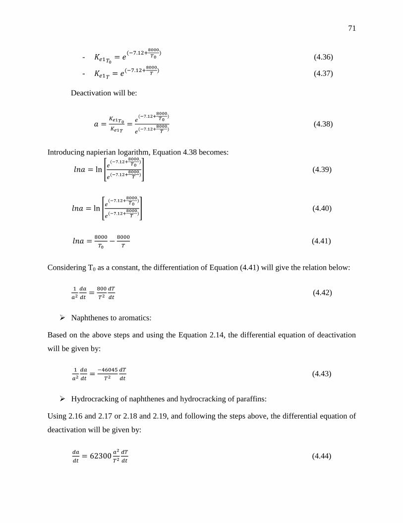
71
- 𝐾𝑒1𝑇0= 𝑒
(−7.12+8000
𝑇0) (4.36)
- 𝐾𝑒1𝑇= 𝑒(−7.12+
8000
𝑇) (4.37)
Deactivation will be:
𝑎 =𝐾𝑒1𝑇0
𝐾𝑒1𝑇
=𝑒
(−7.12+8000
𝑇0)
𝑒(−7.12+
8000𝑇
) (4.38)
Introducing napierian logarithm, Equation 4.38 becomes:
𝑙𝑛𝑎 = ln [𝑒
(−7.12+8000
𝑇0)
𝑒(−7.12+
8000𝑇
)] (4.39)
𝑙𝑛𝑎 = ln [𝑒
(−7.12+8000
𝑇0)
𝑒(−7.12+
8000𝑇
)] (4.40)
𝑙𝑛𝑎 =8000
𝑇0−
8000
𝑇 (4.41)
Considering T0 as a constant, the differentiation of Equation (4.41) will give the relation below:
1
𝑎2
𝑑𝑎
𝑑𝑡=
800
𝑇2
𝑑𝑇
𝑑𝑡 (4.42)
Naphthenes to aromatics:
Based on the above steps and using the Equation 2.14, the differential equation of deactivation
will be given by:
1
𝑎2
𝑑𝑎
𝑑𝑡=
−46045
𝑇2
𝑑𝑇
𝑑𝑡 (4.43)
Hydrocracking of naphthenes and hydrocracking of paraffins:
Using 2.16 and 2.17 or 2.18 and 2.19, and following the steps above, the differential equation of
deactivation will be given by:
𝑑𝑎
𝑑𝑡= 62300
𝑎2
𝑇2
𝑑𝑇
𝑑𝑡 (4.44)
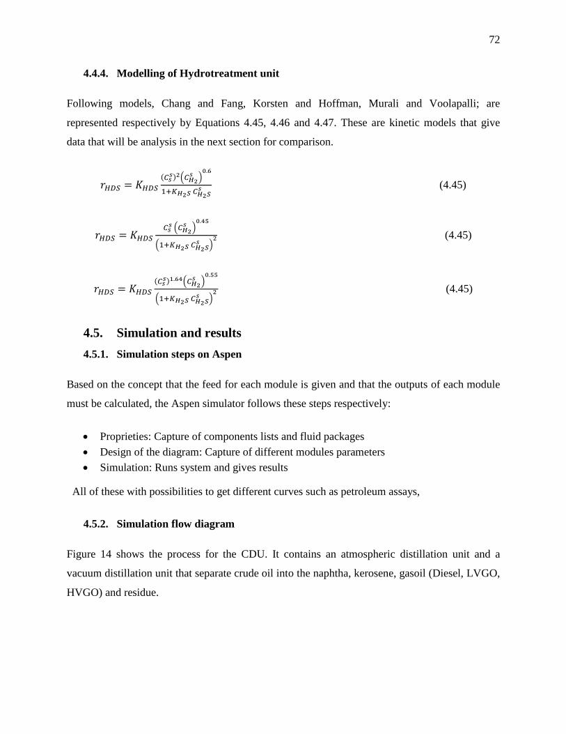
72
4.4.4. Modelling of Hydrotreatment unit
Following models, Chang and Fang, Korsten and Hoffman, Murali and Voolapalli; are
represented respectively by Equations 4.45, 4.46 and 4.47. These are kinetic models that give
data that will be analysis in the next section for comparison.
𝑟𝐻𝐷𝑆 = 𝐾𝐻𝐷𝑆
(𝐶𝑠𝑠)2(𝐶𝐻2
𝑠 )0.6
1+𝐾𝐻2𝑆 𝐶𝐻2𝑆𝑠 (4.45)
𝑟𝐻𝐷𝑆 = 𝐾𝐻𝐷𝑆
𝐶𝑠𝑠 (𝐶𝐻2
𝑠 )0.45
(1+𝐾𝐻2𝑆 𝐶𝐻2𝑆𝑠 )
2 (4.45)
𝑟𝐻𝐷𝑆 = 𝐾𝐻𝐷𝑆
(𝐶𝑠𝑠)1.64(𝐶𝐻2
𝑠 )0.55
(1+𝐾𝐻2𝑆 𝐶𝐻2𝑆𝑠 )
2 (4.45)
4.5. Simulation and results
4.5.1. Simulation steps on Aspen
Based on the concept that the feed for each module is given and that the outputs of each module
must be calculated, the Aspen simulator follows these steps respectively:
Proprieties: Capture of components lists and fluid packages
Design of the diagram: Capture of different modules parameters
Simulation: Runs system and gives results
All of these with possibilities to get different curves such as petroleum assays,
4.5.2. Simulation flow diagram
Figure 14 shows the process for the CDU. It contains an atmospheric distillation unit and a
vacuum distillation unit that separate crude oil into the naphtha, kerosene, gasoil (Diesel, LVGO,
HVGO) and residue.
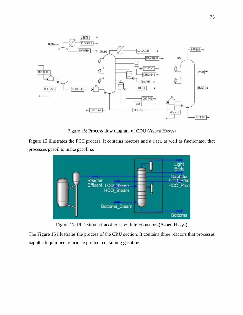
73
Figure 16: Process flow diagram of CDU (Aspen Hysys)
Figure 15 illustrates the FCC process. It contains reactors and a riser, as well as fractionator that
processes gasoil to make gasoline.
Figure 17: PFD simulation of FCC with fractionators (Aspen Hysys)
The Figure 16 illustrates the process of the CRU section. It contains three reactors that processes
naphtha to produce reformate product containing gasoline.
74
Figure 18: Process flow scheme of Catalytic Reforming Unit (Aspen Hysys)
4.5.3. Results of sulphur variation
In this section are represented results of environmental survey of this study focused on the
production of low sulphur gasoline. These results were obtained with the model presented in the
previous sections of our research. Results are illustrated in Table 21:
Table 21: Independent variables
Feed sulphur
wt%
Gasoline / Feed
ratio
Gasoline sulphur reduction
(%)
COR
0.45 to 0.55 7.1 5 4.10
0.60 to 0.75 6.3 10 5.95
0.75 to 0.95 5.6 20 6.01
1.0 to 1.35 4.2 40 8.30
The new regulations which require the sulphur gasoline to be reduced to ppm is the cause of
growth of the FCC process and the common point of all the research used for validation of the
results represented above. The comparison between result obtained and represented in table 21
and the documentary data shows the followings elements:
COR is also an important parameter because its increase leads to an increase in gasoline
reduction. In fact, the gasoline sulphur contents were reduced from 5 to 40%, the COR
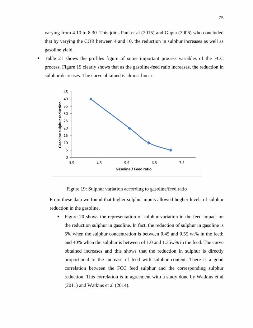
75
varying from 4.10 to 8.30. This joins Paul et al (2015) and Gupta (2006) who concluded
that by varying the COR between 4 and 10, the reduction in sulphur increases as well as
gasoline yield.
Table 21 shows the profiles figure of some important process variables of the FCC
process. Figure 19 clearly shows that as the gasoline-feed ratio increases, the reduction in
sulphur decreases. The curve obtained is almost linear.
Figure 19: Sulphur variation according to gasoline/feed ratio
From these data we found that higher sulphur inputs allowed hogher levels of sulphur
reduction in the gasoline.
Figure 20 shows the representation of sulphur variation in the feed impact on
the reduction sulphur in gasoline. In fact, the reduction of sulphur in gasoline is
5% when the sulphur concentration is between 0.45 and 0.55 wt% in the feed;
and 40% when the sulphur is between of 1.0 and 1.35w% in the feed. The curve
obtained increases and this shows that the reduction in sulphur is directly
proportional to the increase of feed with sulphur content. There is a good
correlation between the FCC feed sulphur and the corresponding sulphur
reduction. This correlation is in agreement with a study done by Watkins et al
(2011) and Watkins et al (2014).
0
5
10
15
20
25
30
35
40
45
3.5 4.5 5.5 6.5 7.5
Gas
olin
e s
ulp
hu
r re
du
ctio
n
Gasoline / Feed ratio
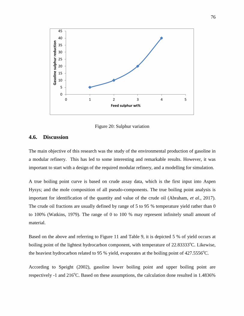
76
Figure 20: Sulphur variation
4.6. Discussion
The main objective of this research was the study of the environmental production of gasoline in
a modular refinery. This has led to some interesting and remarkable results. However, it was
important to start with a design of the required modular refinery, and a modelling for simulation.
A true boiling point curve is based on crude assay data, which is the first input into Aspen
Hysys; and the mole composition of all pseudo-components. The true boiling point analysis is
important for identification of the quantity and value of the crude oil (Abraham, et al., 2017).
The crude oil fractions are usually defined by range of 5 to 95 % temperature yield rather than 0
to 100% (Watkins, 1979). The range of 0 to 100 % may represent infinitely small amount of
material.
Based on the above and referring to Figure 11 and Table 9, it is depicted 5 % of yield occurs at
boiling point of the lightest hydrocarbon component, with temperature of 22.83333oC. Likewise,
the heaviest hydrocarbon related to 95 % yield, evaporates at the boiling point of 427.5556oC.
According to Speight (2002), gasoline lower boiling point and upper boiling point are
respectively -1 and 216oC. Based on these assumptions, the calculation done resulted in 1.4836%
0
5
10
15
20
25
30
35
40
45
0 1 2 3 4 5
Gas
olin
e s
ulp
hu
r re
du
ctio
n
Feed sulphur wt%
77
and 70.6816% as component of the lightest and heaviest gasoline respectively. Thus, this crude
oil can yield up to 69.198 % gasoline.
Figure 12 shows positive disparity in the crude oil. To assert the presence of a gap between
different products cuts that the separation is both viable and simple. Moreover, no significant
overlap that could make distillation difficult for the crude oil studied, no significant complexity
has been added to the CDU design.
For hydraulic analysis in the refinery, especially the design, evaluation and troubleshooting of
piping systems, it is important to study proprieties such as density. Knowing that most crude oil
can be pumped when the SG is in the range of 0.80 (45API) to 0.97 (15 API); Table 11 and
Figure 13 show that LN, HN, K, D and VGO are fluid that can be pumped, excluding the
residue.
The design of crude oil distillation by Manley (1993) also used by Santana and Zemp (2001)
improved thermodynamics process. However, they were limited to certain difficulties such as
unproven and uncertain cost. Some studies proposed short-cut modes for distillation of column,
among them; Gadalla et al (2003) developed optimization approach of existing distillation
processes. Although, there are a lot of studies that proposed different ways of design, some using
software, others using neural network architecture or online application; this study proposed very
basics design method targeting modelling and simulation.
This led us to use a graphical method of designing a distillation column, as graphical method is
suitable for feasibility studies (Flores-Estrella and Iglesias-Silva, 2016). The McCabe and Thiele
graph was then plotted. Published in 1925 by McCabe and Thiele, this method has been found to
be of great use in variety of mass transfer operations (Lichatz, 2019). It can be used for
distillation column design as well as solvent extraction. Using the McCabe and Thiele method
for distillation, it is possible to calculate the number of equilibrium stages required (Gomes,
2007). This method is also convenient to determine the number of stages and reflux that assumes
to be necessary.
78
Thus, our design of crude oil distillation column based on the graphical method above, have
given expected results such as reflux ratio (0.61), number of tray (24), diameter of column (16.83
m) and side strippers volume (5.30 m3).
Most of published information about trickle bed reactors industrial application concerns the
processing with hydrogen of various petroleum fraction (Satterfield, 1975). These applications
are: hydrotreating (hydrotreatment) or hydrofinishing and hydrodesulphurization or
hydrocracking. Generally the trickle bed reactors are operated at high pressure. While in this
work the operating pressure was inspired by Albhari (2001) as follow: 70.31 to 201.92 kg/m2. In
addition, the the weight hourly space velocity was based on previous work, Korsten and
Hoffman (1996), and the value of 0.85 h-1
was used. Results from Askari et al. (2012) and
Korsten Hoffman (1996) study were referenced for the catalyst and industrial bed void value.
This led us first to the Equations 3.28 and 3.29 for calculation of catalyst volume (6.92 m3) and
volume of reactor (13.84 m3); secondly to the sizes of the reactor, that are sectional area (4.15
m2), diameter (2.3 m) and length (16.1 m).
In this study, the fluidized bed reactor was chosen as cracker to design the cracking reactor;
because the fluidized bed is suitable for the production of gasoline. It has been found in the
literature that more attention need to be given to the catalyst in the design as others parameters
must be optimized. Based on a feedstock of 4.66 kg/l (Gary and Handwerk, 2001), the residence
time of 2 second (Lee, 2016), and catalyst data from Bollas et al. (2007) studies; the equations
3.26 and 3.27 were used to obtain: the catalyst-oil ratio (5.95) and catalyst flowrate (44.01 m3/h).
The design of catalytic reforming unit had involved catalyst and reactor design. Typical
operating parameters were reviewed in the literature. Based on Baerns (2013) that inspired
different reactors’ weight hourly specific velocity, on catalyst density and industrial bed void
fraction referred to Askari et al. (2012) and McKetta (1990); calculations could be operated in
Appendix D.2 using Equation 3.28 and 3.29. These lead us to find parameters of each reactor
constituting the reforming unit.
79
Process modelling involves process flow sheet and design; which give importance to the
mathematical modelling economically process design (Khim, 2013). Based on that, this work has
started with the design before carrying on to modelling of refinery’s unit.
After designing a modular process refinery, this study formed mathematical models of crude oil
distillation unit; hydrotreatment; catalytic reforming unit; and fluid catalytic cracking unit.
Because the pressure fluctuation makes the control of distillation unit difficult and reduce it
performance; conventional or advanced distillation control system assume that the column
operates at constant pressure (Minh and Rani, 2009). This was taken into account for the
modelling of crude oil distillation performed in this study. The modelling has also considered
two parameters, namely liquid flow rate and vapour flow rate, as control input of column
distillation as stated in Minh and Rani (2009). Assumptions stated in chapter 3 were mad based
on numerous studies previously published, such as Ann (2014), Jinsa and Ajeesh (2014) or
Stathaki et al. (1985). The assumptions and their implications were applied onto mass balance
and component mass balance. As result developed Equations 4.5 to 4.28 are representing the
process.
The first step in modelling of catalytic cracking was to represent the scheme of reactions
considered in this study. With gasoline as main focus, it was important to consider a number of
lumps that will suit the purpose of this study. Different studies on modelling of FCCU have been
made as of today. As results of previous researches, many have proposed models where
hydrocarbons are grouped or lumped using limited number of reactions (Singh, et al., 2017).
These models are kinetic models that use different number of kinetics lumps: two (Weekman,
1968), three (Weekman, 1969), four (Cristina, 2015), five lumps (Ancheyta-Juarez, 2000;
Bollas), six (Ancheyta, 2002), seven (Heydari, 2010) height (Sani, 2018), seventeen (Singh, et
al., 2017), etc. in this study 4 kinetics lumps were considered as vacuum gasoil, coke, light gases
and gasoline are the considered group of hydrocarbons.
Due to the complexity of the feed coming into the catalytic reformer and various reactions that
take place, kinetic models are very difficult to obtain. Thus, kinetic lumps are also used for
reforming of such unit. Throughout the years several models been developed with aim to make a
80
better representation of the kinetics of catalytic reforming reactions. Among them we mentioned,
Smith (1959), Padmavathi and Chaudhuri (1997). Referring to Ancheyta et al. (2001), a semi-
regenerative reactor was taken into account in this study in order to allow an increase in severity.
Furthermore, focusing on gasoline the modelling of reforming has considered Smith model. The
main focus on modelling of reforming unit was to develop a model based on activation. Knowing
the rates constant expressions, it can be used to get deactivation; calculus devices, especially
napierian logarithm have been used to develop a differential equation as model of catalytic
reforming unit. Finally modelling of hydrotreatment unit was based on previous works. This
gave us reasonable reduction of sulphur. Therefore, the Murali and Voolapalli kinetic model
approches the experimental data.
Reducing the sulphur concentration in products is still important to comply with the regulations
to reduce gas emissions emanated from combustion of fuel. This study looked onto environment
impact of sulphur concentration using simulation. The data have been analyzed to find out how
sulphur content changes in a specific products, for instance the gasoline.
It is clear that an appropriate study on FCCU and HTU must be carried outbefore implementing
data on the process. Referring to Letzsch et al. (2009) that states that the range of COR is
normally 4:1 to 9:1, the modular refinery simulation is a success because of the results obtained
(4.10:1 to 8.30:1; with a high variation of sulphur in gasoline. This can meet different regulations
mentioned in the literature.
81
CHAPTER 5
CONCLUSION AND RECOMMENDATION
5.1. Conclusions
The objectives of this study are the design and simulation of a modular refinery using Aspen
Hysys, as well as to investigate the environmental influence of the process on the product
compositions. The characterization of the fed crude oil then becomes essential, as the design of
different units based on the characterized oil. Below are the designed variables used for this
investigation:
Reflux, number of trays, column height, column diameter, feed tray position and stripers
volume for the CDU
Volume, sectional area, diameter and length for HTU
Volume and mass catalyst for CRU
Volume and flow rate of catalyst for FCCU
The crude oil and its different cuts characterization results showed a clear variation in all
properties. The refinery was successfully simulated and validated using Aspen Hysys simulation
tool. This software was used to determine the amount of sulphur in gasoline for further study,
such as environmental investigation of the process. The results obtained give enough information
that are specifications of the crude oil required for the design.
The designs have been performed using the specifications obtained previously. The theoretical
design gives a specified details and information of the main refinery units that have been targeted
in this study. The data obtained after calculation represent an advantage and useful results for the
design, in particular material and energy balances.
A modular refinery with a processing capacity of 12,000.00 bbl/day was designed and a detailed
equipment design using numerical calculations was carried out. Although the simulation gave
more detailed and effective results, numerical design technique made possible to better compare
82
the Aspen Hysys simulation. Equipment design includes column (number of trays 24, reflux ratio
0.51 and column height: 16.83m), side strippers (volume 5.30 m3), trickle bed reactor (catalyst
volume 6.92 m3, reactor volume 13.84 m
3, sectional area 4.15 m
3, diameter 2.30 m
3 and length
16.1m), catalytic reforming reactor (reactor 1 catalyst volume 3.69 m3, reactor 2 catalyst volume
5.90 m3, reactor 1 catalyst volume 26.82 m
3, reactor 1 volume 7.38 m
3, reactor 2 volume 11.80
m3 and reactor 3 volume 53.64 m
3) and catalytic cracking reactor (catalyst flowrate 44.01 m
3/h,
catalyst rate 0.006 m3/sec and catalyst to oil ratio 5.95).
The Aspen Hysys simulation of the model obtained by designing helps to provide a complete
evaluation of the equipment. This survey increased the production of gasoline using Aspen
Hysys software and provided details on the environmental impact.
Environmental results presented in this study are in good agreement with results presented by
author mentioned in literature review and methodology.
The improvement of refineries definitely needs techniques such as modelling and simulation.
The use of modelling in different studies always adds useful data in this field. High subjective
errors in evaluation of refinery project are avoided when simulation is coupled with modelling.
5.2. Recommendations
During the course of this study, various considerations were made to study the environment
effects of sulphur in products. The data obtained in this research was not focused entirely on all
environmental aspects. However, data on influence of sulphur on the environment were
sufficient, although some empirical calculations were made from the beginning. In this respect,
future studies are recommended to implement a pilot plant, in order to find the best parameter
values for maximum production and an advanced environmental study on refinery.
This study performed a specific case study provided by the design. Because refineries have
different configurations and give differences in products, more cases of modular refineries
should be investigated. It is even very important to consider the configuration of a large-scale
refinery. The configuration and scale can influence the concentration of sulphur in gasoline. The
catalyst amount must be designed according to the feedstock data. It is possible to study the

83
influence of configuration and scale by analysing different cases with different modular
refineries.
Deviations from the design specifications and changes operating parameters may occur due to
the state of feed mixture and feed composition of crude oil. This can jeopardize the purpose of
the refinery. It is then recommended to consider this factor in future studies.
84
REFERENCES
Abdullah, Z., Aziz, N. and Ahmad, Z. (2007) “Nonlinear Modelling Application in Distillation
Column”, Chemical Product and Process modelling, 2(3), p.12.
Abraham, J.M., Babu, A., Manoj, K., Ahamed, K., Raj, G., Arunachaleswara, P.R. and Kanna,
R. (2017) “Correlation of True Boiling Point of Crude Oil”, International Refereed Journal of
Engineering and Science (IRJES), pp. 45-49.
Abubakar, A.; Mohammed-Dabo, I.A. and Ahmed, A.S. (2016) “reduction of Sulphur Content
of urals Crude Oil Prior to Processing using Oxidative Desulphurization”, Nigerian journal of
Basic and apllied Science, 24(1): 19-24.
Adefarati, F. and Chigbu, P. (2017) The continuous advocacy for Modular refineries in Nigeria:
time for all hands to be on deck, Energy & Natural Resources Department, SPA Ajibade & Co,
Lagos, Nigeria.
Akpa, J.G. and Umuze, O.D. (2013) “Simulation of a Multi-component Crude Distillation
Column”, American J. of Scientific and Industrial Research, 4(4), pp.366-377.
Alattas, A.M., Grossmann, I.E. and Palou-Rivera, I. (2012) “Refinery production planning:
Multiperiod MNLP With CDU model”, Industrial & Engineering Chemistry Research, 51(39),
pp.12852–12861.
Albahri, T (2001) “Petroleum refining-Chapter 8: Desulfurization”, Kuwait University.
Albhari, T (2008) “Petroleum refining-chapter 8: Desulphurization”
www.albhari.info/Refinery/Chapter08%20-%20Desulfurization.pdf [2017, June 25].
Al-Malki, A. (2004) “Desulfurization of Gasoline and diesel Fuels, Using Non-Hydrogen
consuming Techniques”, Master of Science Dissertation, King Fahed University of Petroleum
and Minerals.
85
Ancheyta, J (2011) “Modelling and Simulation Catalytic Reactors for Petroleum Refining”, John
Wiley & Sons, Inc, Hoboken, New Jersey.
Ancheyta, J. and Sotelo, R. (2002) “Kinetic modeling of vacuum gas oil catalytic
cracking”, Revista de la Sociedad Química de México, 46(1), pp.38-42.
Ancheyta, J; Villafuerte, ME; Díaz, G.L; González, AE (2001) “Modelling and Simulation of
Four Catalytic Reactors in Series for Naphtha Reforming”, Energy Fuels, 15, 887-893.
Ancheyta-Juarez, J. and Sotelo-Boyas, R. (2000) “Estimation of kinetic constants of a five-lump
model for fluid catalytic cracking process using simpler sub-models”, Energy & fuels, 14(6),
pp.1226-1231.
Ann, I.W.F. (2014) “Modelling and simulation of distillation column”, BEng Chem Thesis,
Universiti Malaysia Pahang.
Arani, HM, Shokri, S and Shirvani (2010) “Dynamic Modelling and Simulation of Catalytic
Naphtha Reforming”, International Journal of Chemical Engineering and Applications, 1(2),
p.159.
Askari, A; Karimi, H; Rahimi, MR and Ghanbari M (2012) “Simulation and modelling of
catalytic reforming process”, Petrol. Coal, 54(1), pp.76-84.
AspenTech (2009) “Getting Started Modelling Petroleum Processes”, Aspen Technology, Inc.
Burlington, USA.http://www.aspentech.com [2017, May 16].
Backhurst, J. R., Coulson, J. M., Harker, J. H., & Richardson, J. F. (1999) “Fluid Flow, Heat
Transfer and Mass Transfer”, Oxford: Butterworth-Heinemann.
Barbosa, AC; Lopes GC; Rosa LM; Mori, M and Martignoni, WP (2013) “Three dimensional
simulation of catalytic cracking reactions in an industrial scale riser using a 11-lump kinetic”, In
AIDIC Conference Series, 11, 31-40.
86
Barletta, T., White, S. and Chunangad, K. (2012) “Designing a crude unit heat exchanger
network”, Petroleum Technology Quarterly, 16, p.3.
“Basic knowledge Distillation”,
http://www.gunt.de/images/download/distillation_rectification_english.pdf [2017, January 02].
Behmiri, NB and Manso, JPR (2014) “The linkage between crude oil consumption and economic
growth in Latin America: The panel framework investigations for multiple regions”, Energy, vol.
72, no. 1, pp. 233-241.
Bhende, SG and Patil, KD (2014) “Modelling and simulation for FCC unit for the estimation of
gasoline production”, International Journal of Chemical Sciences and Applications, Vol 5, Issue
2, pp 38-45.
Bollas, G.M., Lappas, A.A., Iastridis, D.K. and Vasalos, I.A. (2007) “Five-lump Kinetic model
with selective catalyst deactivation for the prediction of the product selectivity in the fluid
catalyst process”, Catalysis Today, Volume 127, pp. 31-43.
Boston, J. F. and Sullivan, S. L. (1974) “A New Class of Solution Methods for Multi-component,
Multistage Separation Processes”, The Canadian Journal of Chemical Engineering, 52(1), pp.52-
63.
Brooks, B. A. (1993) “Modelling of a Distillation Column Using Bond Graphs”, M.Sc. Thesis,
University of Arizona, 70-88.
Brown, K.B.; Maxwell, R.V. and Shumwau, M.D. (2003), Modular Oil Refinery, US. Patent
WO2003031012A1.
Bunse, K; Vodicka, M; Schönsleben, P; Brülhart, M and Ernst, FO (2011) “Integrating energy
efficiency performance in production management–gap analysis between industrial needs and
scientific literature”, Journal of Cleaner Production, 19(6), pp.667-679.
Caballero S.B. (2014) “Logic hybrid simulation-optimization algorithm for distillation design”,
Computers & Chemical Engineering.
87
CenAm Energy Partners (2012) “The Case for Modular Mini-Refineries”, Internal Company
Report. CenAm Energy Partners S.A, Panama City, Panama
Cheremisinoff, NP and Rosenfeld, P.E (2009) “Handbook of pollution prevention and cleaner
production Vol. 1: Best practices in the petroleum industry”, William Andrew.
Cristina, P. (2015) “Four–Lump Kinetic Model vs. Three-Lump Kinetic Model for the Fluid
Catalytic Cracking Riser Reactor”, Procedia Engineering, 100, pp.602-608.
Couper, J.R., Penney W.R, Fair, J.R. and Walas, S.M. (2012) “Chemical Process Equipment
Selection and Design”, Butterworth-Heinemann, Third Edition.
Cournoyer, A., Couture, G., Couture, J-F., Ferland, M., Fontaine, A., Gervais, O., Giroux, F.,
Laplante, A., Lapointe-Garant, P-P., Morin, V. and Vallières, S. (2005) “Rapport Final- Équipe
A - Raffinerie intégrée’’, Final Report, Département de génie chimique, Université de
Sherbrooke, Quebec, Canada.
Cross, P; Desrochers, P and Shimizu, H (2013) “The economics of Petroleum Refining,
Understanding the business of processing crude oil into fuels and other value products”,
Canadian Fuels Association, Ottawa, Canada.
Daneshvar, MR and Fatemi, S (2011) “Mathematical Modelling and Simulation of Hydrotreating
(HDS, HDN and HAD) of Gas oil in Commercial Trickle-bed Reactor”, In 7th International
Chemical Engineering Congress & Exhibition.
De la Paz-Zavala, C., Burgos-Vázquez, E., Rodríguez-Rodríguez, J.E. and Ramirez-Verduzco
(2013) “Ultra low sulfur diesel simulation. Application to commercials units”, Fuel 110, pages
227-234.
DEA- RSA (2010) “National Climate Change Response Green Paper”, Department of
Environmental Affairs.
Doronin, VP and Sorokina, TP (2007) “Chemical design of cracking catalysts”, Russian Journal
of General Chemistry, 77(12), pp.2224-2231.
88
Douani, M., Ouadjenia, F. and Terkhi, S. (2007a) “Distillation of a complex mixture. Part I:
High Pressure Distillation Coulmn analysis: Modelling and simulation”, Entropy, 9, (2), 58-72.
Douani, M., Terkhi, S. and Ouadjenia F. (2007b) “Distillation of a Complex Mixture. Part II:
Performance Analysis of a Distillation Column Using Exergy”, Entropy, 9, pp 137-151.
Douglas, J. (1988) “Conceptual Design of Chemical Process”, MacGraw-Hill, Inc, section A-3.
Dreher, T. (2016) “Electrostatic Desalter Optimisation”, MI lecture note series, 67, pp.24-29.
Ejikeme-Ugwu, E (2012) “Planning for the integrated refinery subsystems”, Ph.D. Thesis,
Cranfield University, United Kingdom.
El-Hadi, D (2015) “Comparative Study of the Characterization Factors for Hydrocarbon Types
of Petroleum Fluids Fractions”, Journal of Petroleum Science Research.
Energy Information Administration “EIA” (2014) “Independent statistics and analysis”, US
Department of Energy.
Energy Information Agency “EIA” (2014) “Products made from a Barrel of Oil”, US
Department of Energy.
Environmental Protection Agency “EPA” (1995) “Compilation of air pollutant emissions factors
Volume 1: Stationary Point and Area Sources”, US Department of Environment, AP 42, Fifth
edition.
Eβer, J.; Wassercheid, P and Jess, A (2004) “Deep desulfurization of oil refinery streams by
extraction with ionic liquids”, Green Chemistry.
Fagan, A (1991) “An Introduction to the petroleum industry”,Terminology, vol. 1, p. 1.
Fahim, MA; Al-Sahhaf, TA and Elkilani, A (2010) “Fundamentals of petroleum refining”,
Elsevier, pp.1-32.
89
Ferreira, C; Marques, J; Tayakout, M; Guibard I; Lemos, F; Toulhoat H and Ramoa Ribeiro, F
(2009) “Modelling residue hydrotreating”, In 20th International Symposium in Chemical
Reaction, Chemical Engineering science: Engineering—Green Chemical Reaction Engineering
for a Sustainable Future, pp. 322–329.
Fetter-Pruneda, E., Borrell Escobedo, E.R. and Garfias Vázquez, F.J. (2005) “Optimum
temperature in the electrostatic desalting of Maya crude oil”, Journal of the Mexican Chemical
Society, 49(1), pp.14-19.
Flores-Estrella, R.A. and Iglesias-Silva, G.A. (2016) “Reactive McCabe-Thiele: Short cut
method including reactive vapor-liquid efficiency”, Revista Mexicana de Ingeniería
Química, 15(1), pp.193-207.
Fuente, J. R. (2015) “Equipment Sizing and Costing”, In J. R. Fuente, Chemical Process Design,
Cantabria: open course ware, pp. 2-30.
Gadalla, M., Jobson, M. and Smith, R. (2003) “Optimization of existing heat-integrated refinery
distillation systems”, Chemical Engineering Research and Design, 81(1), pp.147-152.
Gañí, R., Ruiz, C.A. and Cameron, I.T. (1986) “A generalized model for distillation columns-I:
Model description and applications”, Computers & chemical engineering, 10(3), pp.181-198.
Gary, JH and Handwerk, GE (2001) “Petroleum Refining Technology and Economics”, Marcel
Dekker Inc. New York.
Gary, JH; Handwerk, GE and Kaiser, MJ (2007) “Petroleum refining: technology and
economics.4th
”, CRC press.
Green D. and Perry R. (2007) “Perry’s Chemical Engineer’s Handbook”, Eight Edition,
McGraw-Hill.
Gomes, J.F.P. (2007) “Reflections on the use of the Mccabe and Thiele method”, Revista
Ciências & Tecnologia, Ano 1, n. 1.
90
Gupta, R.S. (2006) “Modelling and Simulation of Fluid Catalytic Cracking Unit”, PhD Thesis,
Thapar Institute of Engineering and Technology, India.
Han, IS; Riggs, J.B and Chung, CB (2000) “Modelling of a fluidized catalytic process”,
Computers & Chemical Engineering and Processing, 24(2000), pp.1681-1687.
Harbert, W.D. (1978) “Preflash saves heat in crude unit”, Hydrocarbon Processing, 57(7),
pp.123-125.
Haydary, J and Pavlík, T (2009) “Steady-state and dynamic simulation of crude oil distillation
using Aspen Plus and Aspen Dynamics”, Petroleum and Coal, 51(2), p.100.
Heydari, M., AleEbrahim, H. and Dabir, B., 2010. Study of seven-lump kinetic model in the
fluid catalytic cracking unit American Journal of Applied Sciences, 7(1), p.71.
Heydari M., AleEbrahim H. and Dabir B. (2010) “Study of seven-Lump Kinetic Model in the
Fluid Catalytic Cracking Unit”, American Journal of Applied Sciences, 7 (1): 71-76.
Hug, I (1998) “Design Control Studies on the Fluid Catalytic Cracking Process”, Thesis in
partial fulfilment of the requirement of Doctor of philosophy, California Institute of Technology,
Pasadena, California, pp. 1234.
Ibrahim, H.A.H. (2014) “Design of Fractionation Columns”, In MATLAB Applications for the
Practical Engineer, DOI: 10.5772/57249.
Ibsen, K (2006) “Equipment Design and Cost Estimation for small Modular Biomass Systems,
Synthesis Gas Cleanup, and Oxygen Separation Equipment - Task 1: Cost Estimates of small
Modular Systems”, National Renewable Energy Laboratory, Midwest Research Institute,
Battellle, Subcontract report NREL/SR-510-39943. Contract No, Sans Francisco, California.
Ilkhaani, S (2009) “Modelling and optimization of crude oil desalting”. Master thesis, University
of Waterloo, Department of Chemical Engineering, Waterloo, Ontario, Canda.
91
International Energy Agency “IEA” (2016) “CO2 emissions from fuel combustion-highlights”,
www.iea.org/statistics/onlinedataservice/ [2017, July 29].
Ivakpour, J. and Kasiri, N. (2008) “Improve speed and convergence of distillation column
simulation”, Hydrocarbon Process, 87(10), pp.75-79.
Jaroslav, J., Hlavacek, V. and Kubicek, M. (1973) “Calculation of Multistage Countercurrent
Separation Processes-I. Multi-component Multi-stage Rectification by Differentiation with
Respect to an Actual Parameter (J)”, Chem. Eng. Sci., 28(10), 1555-1563.
Jarullah, A.T., (2012) “Kinetic Modelling Simulation and Optimal Operation of Trickle Bed
Reactor for Hydrotreating of Crude Oil. Kinetic Parameters Estimation of Hydrotreating
Reactions in Trickle Bed Reactor (TBR) via Pilot Plant Experiments; Optimal Design and
Operation of an Industrial TBR with Heat Integration and Economic Evaluation”, Doctoral
dissertation, University of Bradford.
Jechura, J (2017) “Refinery Feedstocks and Products–Proprieties and Specifications”, Colorado
School of mines, USA.
Jelinet J. and Hlavecek V. (1975) “Mathematical Modelling of the Rectification Process”,
International Chemical Engineering, 15(3) 487-494.
Jinsa M. and Ajeesh K.N. (2014) “Distillation composition control of binary distillation
column”, Journal Impact Factor, Volume 5, Issue 3, pp 79-85.
Jones, D.S. and Pujadó, P.P. eds. (2006) “Handbook of petroleum processing”, Springer Science
& Business Media, p.p. 1-109.
Kane, RD (2006) “Corrosion in Petroleum Refining and Petrochemical Operations”, Corrosion:
Environments and Industries, vol 13C, p 967-1014.
Kemp, I. C. (2007) “Pinch Analysis and Process Integration-A User Guide on Process
Integration for the Efficient Use of Energy”, Oxford.Butterworth-Heinemann.
92
Khim, TW (2013) “Dynamic modelling of crude distillation unit”, Bachelor of Engineering
dissertation, Universiti Malaysia Pahang.
Kister, H. (1992) “Distillation design (vol1)”, McGraw-Hill Professional.
Kodjak, D (2015) “Policies to reduce fuel consumption, air pollution, and carbon emissions from
vehicles in G20 nations”, The International Council on Clean Transportation, Washington, D.C.
http://www.theicct.org/policies-reduce-fuel-consumption-air-pollution-andcarbon-emissions-
vehicles-g20-nations [2017, October 10].
Kolmetz, K. and Sari, R.M. (2016) “Refinery atmospheric crude tower selection and sizing
(Engineering Design Guideline)”, Kolmetz Handbook of Process Equipment Design, Malaysia,
pp 1-164.
Kumar, V., Sharma, A., Chowdhury, I.R., Ganguly, S. and Saraf, D.N. (2001) “A crude
distillation unit model suitable for online applications”, Fuel processing technology, 73(1), pp.1-
21.
Lee, Q.F (2016) “Fluid Catalytic cracking”, Chemical and Biological Engineering, University of
British Columbia, Canada.
Leffler, W.L. (1985) “Petroleum refining for nontechnical person, 2nd Edition”, PennWell
Books, ISBN 0-87814-280-0.
Lekan, T.P., Gutti, B. and Alfred, A.S. (2013) “A review of an expert system design for crude oil
distillation column using the neural networks model and process optimization and control using
genetic algorithm framework”, Advances in Chemical Engineering and Science, 3, pp.164-170.
Letzsch, W., Santner, C. and Tragesser, S. (2009) “FCC reactor design: Part II”, Petroleum
Technology Quarterly, (1), p.25-29.
Li, W; Hui, CW and Li, A (2005) “Integrating CDU, FCC and product blending models into
refinery planning”, Computers & chemical engineering, 29(9), pp.2010-2028.
93
Liang, KM; Guo, HY and Pan, SW (2005) “A study on naphtha catalytic reforming reactor
simulation and analysis”, Journal of Zhejiang University, Science.B, 6(6), p.590.
Lichatz, T.A., “Dr. "Angelo Lucia’s Tutorials on Distillation”, National Science Foundation,
accessed 2019-12-16, https://personal.egr.uri.edu/lucia/tutorials/tutorial2.html
Linninger, A., Senior Design CHE 396, Innovations Solutions.
Liu, L (2015) “Molecular Characterization and Modelling for Refining Processes”, Ph.D.
Thesis, University of Manchester, England.
López, D.C., Mahecha, C.A., Hoyos, L.J., Acevedo, L. and Villamizar, J.F. (2009)
“Optimization model of a system of crude oil distillation units with heat integration and
metamodelling”, CT&F-Ciencia,Tecnología y Futuro, 3(5), pp.159-173.
Manjumdor, S.K. and Das, C. (2012) “Mass transfer operation 1-Distillation”, National
programme on Technology Enhanced Learning,s Indian Institute of Technology Guwahati.
Assam, India.
Manley, D.B., 1(993) “Waste minimization through improved process thermodynamics: crude
oil fractionation”, The University of Missouri, Rolla, Missouri.
McCabe, W.L., Smith, J.C. and Harriott, P (1993) “Unit Operations of Chemical Engineering
Fifth Edition”, MacGraw-Hill.
McCabe-Thiele, VAXA Software, PTTD, Version 1.8.0, www.vaxasoftare.com
McCain, WD (1990) “The properties of petroleum fluids”, PennWell Books, Tulsa.
McSweeney, R. and Timeperley, J. (2018) “The Carbon Brief Profile: South Africa”,
https://www.carbonbrief.org/the-carbon-brief-profile-south-africa.
Merdrignac, I and Espinat, D (2007) “Physicochemical characterization of petroleum fractions:
the state of the art”, Oil & Gas Science and Technology-Revue de l'IFP, 62(1), pp.7-32.
94
Minh, V.T. and Rani, A.M.A. (2009) “Modelling and Control of Distillation Column in
Petroleum Process”, Mathematical Problems in Engineering, Article ID 404702
Moses, J.R.L. (2011) “Petroleum Refining: Modular versus Conventional Refineries”,
www.vanguardngr.com/2011/10/petroleum-refining-modular-versus-conventional-refineries/
[2017, January 2011]
Mustapha, D., Fatima, O. and Sabria, T. (2007) “Distillation of a Complex Mixture. Part I: High
Pressure Distillation Column Analysis: Modelling and Simulation”, Entropy, 9(2), pp.58-72.
Muhsin, W.A.S.; Zhang, J. and Lee, J. (2016) Modelling and Optimisation of Crude oil
Hydrotreating Process Using neural network, Chemical Engineering transactions, 52, 211-216,
DOI: 10.3030 ICET1652036.
Naré, H and Kamakaté, F (2017) “Developing a roadmap for adoption of clean fuel and vehicle
standards in Southern and Western Africa”, International Council on Clean Transportation.
Odebunmi, E.O.; Ogunsakin, E.A. and Ilukhor, P.E.P. (2002) “Characterization of crude oils and
petroleum products: elution liquid chromatographic separation and gas chromatographic analysis
of crude oils and petroleum products”, Bulletin of the Chemical Society of Ethiopia, 16(2),
pp.115-132.
Ogundari, IO; Akinwale, Y; Adepoju AO and Akarakiri, JB (2012) “The modular Petroleum
Alternative as an Energy Security and Environmental Sustainability Strategy in Nigeria: A
Technology Policy Assessment”, 3rd Technology Management for Directors of Science and
Technology, Bayelsa State, Nigeria.
Pahwa, R and Gupta, R (2016) “CFD Modelling of FCC Riser Reactor”, Int. Res. J. eng.
Technol., 3(2), pp. 206-209.
Pant, K.K. and Kunzru, D. (2015) “Pretroleum refinery engineering-Design concept of crude oil
distillation column design”, National programme on Technology Enhanced Learning. Indian
Institute of Technology Delhi.
95
Parkash, S (2003) “Refinning Process Handbook”, Gulf publishing, New York.
Partnership for Clean Fuels and Vehicles “PCFV” (2015) “Clean fuels and vehicles regulatory
toolkit”, United Nations-Environmental Protection agency (UNEP), Naerobi, Kenya.
Paul, D; Thakur, R.S. and Chaudhari, P.K. (2015) Simulation of FCC Riser Reactor Using Five
Lump model, International Journal of ChemTech Research, ISSN: 0974-4290, vol. 8, No 6, pp
750-758.
PetroWiki, Oil demislsification, viewed 14th Frbruary, 2017,
<http://petrowiki.org/Oil_demulsification>
Prince, R.M. (2003) “Distillation, retrieved from lectures”,
http://facstaff.cbu.edu/rprice/lectures/distill7.html
Putter, A (2015) “The Need for Southern African Liquid Fuels Production”,
www.otctoolkits.com/the-need-for-southern-african-liquid-fuels-production/ [2017, October 02].
Rahim, K and Ben-Rahla, S. (2012) “Calcul de vérification et optimisation des paramètres de
fonctionnement de la colonne de Stabilisation PX0-CB-21-01 de l’UTBS”, Mémoire de Master,
University Mohamed KhiderBiskar, Algeria.
Ramesh, K., Aziz, N., Shukor, S.A. and Ramasamy, M. (2007) “Dynamic rate-based and
equilibrium model approaches for continuous tray distillation column”, Journal of Applied
Science Research, 3(12), pp.2030-2041.
Rao, R.M., Rengaswamy, R; Suresh, A.K. and Balaraman, KS (2004) “Industrial experience
with object-oriented modelling: FCC case study”, Chemical Engineering Research and Design,
82(4), pp.527-552.
Ratshomo, K. and Nembahe, R. (2015) “Overview of petroleum and diesel market in South
Africa between 2002 and 2013”, Energy data collection management and analysis, 1st Edition.
96
Reyes-Labarta, J.A. (2010) “Métodos para el cálculo de operaciones de separaciónmultietapa en
mezclasmulticomponentes”, University of Alicant.
Riazi, M.R. (2005) “Characterization and properties of petroleum fractions (vol. 50)”, ASTM
international.
Richmond, B. (2006), “Introduction to Data analysis Handbook”, Academy for Educational
development, Washington.
Rivotti, P.M.N. (2009) “Modelling of vacuum residue hydrotreatment. Impact of the feedstock
description on model output”, Master degree Dissertation, Instituto Superior Técnico, page 16.
Rosendo, M. L. (2003) “Simulation of Multi-component Multistage Vapor-Liquid Separations,
An Improved Algorithm using the Wang-Henke Tridiagonal Matrix Method”, Ind. Eng. Chem.
Res., 42(1), 175-182.
Sadeghbeigi, R. (2000) “Fluid catalytic cracking handbook: Design, Operation and
Troubleshooting of FCC Facilities”, Butterworth-Heinemann, 2nd Edition.
Sadeghbeigi, R. (2012) “Fluid catalytic cracking handbook: An expert guide to the practical
operation, design, and optimization of FCC units”, Elsevier, Waltham.
Sani, A.G., Ebrahim, H.A. and Azarhoosh, M.J. (2018) “8-Lump kinetic model for fluid catalytic
cracking with olefin detailed distribution study’, Fuel, 225, pp.322-335.
Santana, E.I. and Zemp, R.J. (2001) “Thermodynamic Analysis of a Crude-Oil Fractionating
Process”, In 4th Mercosur Congress on Process Systems Engineering, vol. 21, pp. 523-528.
SAPIA (2016) “South African Petroleum Industry Association, cleaner fuels II”,
http://www.sapia.org.za/Key-Issues/Cleaner-fuels-II, [2017, June 17]
Satterfield, C.N. (1975), “Trickle-bed reactors”, AIChE Journal, vol 21, no2.
97
Saunders, M., Lewis, P. and Thornhill, A. (2009), “Research methods for business students.5th
Edition”, Harlow, England: Prentice Hall. https://is.vsfs.cz/el/6410/leto2014/
BA_BSeBM/um/Research_Methods_for_Business_Students__5th_Edition.pdf [25/10/2018].
Seader, JD, Henley, EJ and Roper, DK (2011) “Separation process principles, 3rd
Edition”, John
Wiley & Sons Incorporated, pp. 1-2.
Sharma, P. (2018) “Developing an Online Predictor to Predict Sulfur Concentration for HDS
Unit”, Master of Engineering Dissertation, Memorial University of Newfoundland.
Sharma, S. and Ghosh, R. (2016) “Designing and Process Simulation of A Single Column Crude
Distillation Unit for Refineries”, Imperial Journal of Interdisciplinary Research (IJIR), Vol 2, P.
985.
Shokri, S., Marvast, M.A. and Tajerian, M. (2007) “Production of ultra low sulphur diesel:
Simulation and software development”, Petroleum and Coal, ISSN 1337-7027.
Singh, B., Sahu, S., Dimri, N., Dasila, P.K., Parekh, A.A., Gupta, S.K. and Das, A.K. (2017)
“Seventeen-lump model for the simulation of an industrial fluid catalytic cracking unit
(FCCU)”, Sādhanā, 42(11), pp.1965-1978.
Sinnot, R. K. (2005) “Chemical Engineering Design”, Oxford: Elsevier Butterworth-Heinemann.
Sittig, M. (1978) “Petroleum Refining Industry Energy Saving and Environmental Control”,
Noyes Data Corporation, New Jersey.
Smith, R.B. (1959) “Kinetic analysis of naphtha reforming with platinum catalyst”, Chem. Eng.
Prog, 55(6), pp.76-80.
Solomon, A. F. (1981) “Recent Advances in the Study of Multicomponent Distillation", B.Sc.
Thesis, Chemical Engineering Department, University of Lagos, Nigeria.
Song, C. (2003) “An overview of new approaches to deep desulfurization for ultra-clean
gasoline, Diesel Fuel and Jet Fuel”, Catalyst today, Volume 86, issues 1-4, pages 211-263.
98
Souck, J.B. (2012) “Modelling of crude oil distillation”, MSc Thesis, KTH Royal Institute of
Technology, Stockholm, Sweden.
Speight, JG (2002) “Handbook of petroleum product analysis”, New York, John Wiley & Sons,
pp. 1-66.
Speight, JG (2006) “The chemistry and technology of petroleum”, Laramie, CRC press, pp. 31-
46.
Sridhar, L.N. and Lucia, A. (1990) “Tearing algorithms for separation process simulation (J)”,
Computer Chemical Engineering, 14(8), 901-905.
Stathaki, A., Mellichamp, D.A. and Seborg, D.E. (1985) “Dynamic Simulation of a
Multicomponent Distillation Column with Asymetric Dynamics”, The Canadian Journal of
Chemical Engineering, volume 63.
Taskar, UM (1996) “Modelling and optimization of a catalytic naphtha reformer”, Ph.D.
dissertation, Texas Tech University.
Thambiran, T. and Diab, R.D. (2011) “Air pollution and climate change co-benefit opportunities
in the road transportation sector in Durban, South Africa”, Atmospheric Environment, 45(16), pp.
2683-2689. doi:10.1016/j.atmosenv.2011.02.059
Tissot, B.P .and Welte, D.H. (1984) “From kerogen to petroleum-In Petroleum Formation and
Occurrence”, Springer Berlin Heidelberg, pp. 160-198.
Vafajoo, L., Ganjian, K. and Fattahi, M. (2012) “Influence of key parameters on crude oil
desalting: An experimental and theoretical study”, Journal of Petroleum Science and
Engineering, 90, pp.107-111.
Vanmali, KH (2014) “Improving refinery productivity through better utilization of crude oil
blending using linear programming”, MSc research report, University of the Witwatersrand,
Johannesburg.
99
Vathi, G.P. and Chaudhuri, K.K. (1997) “Modelling and simulation of commercial catalytic
naphtha reformers”, The Canadian Journal of Chemical Engineering, 75(5), pp.930-937.
Wakeford, JJ (2012) “Socioeconomic implications of global oil depletion for South Africa:
vulnerabilities, impacts and transition to sustainability”, Doctorat of Philosophy Dissertation.
Stellenbosch University.
Watkins, B; Haley, J. and Schiller, R. (2014) Meeting Tier 3 Gasoline Sulfur Regulations, Grace
Catalysts Technologies Catalagram, Issue No 114/2014, p. 36-39.
Watkins, B; Olsen, C. and Hunt, D. (2011) Balancing the Need for low sulphur FCC Products
and Increasing FCC LCO Yields by Applying Advanced Technology for Cat Feed
Hydrotreating, NPRA Annual Meeting, Issue No 109/2011, p. 38-48.
Watkins, R. N. (1979) “Petroleum Refinery Distillation”, Second Edition, Gulf Publishing
Company, Houston.
Wauquier, JP (1994) “Le raffinage du pétrole-Tome 1-Pétrole brut, Produits pétroliers. Schémas
de fabrication (Vol. 1) ”, Editions Technip, Paris.
Weekman Jr, V.W. (1968) “Model of catalytic cracking conversion in fixed, moving, and fluid-
bed reactors”, Industrial & Engineering Chemistry Process Design and Development, 7(1),
pp.90-95.
Weekman Jr, V.W. (1969) “Kinetics and dynamics of catalytic cracking selectivity in fixed-bed
reactors” Industrial & Engineering Chemistry Process Design and Development, 8(3), pp.385-
391.
Wlazlowski, S; Hagströmer, B. and Giulietti, M. (2001) “Causality in crude oil prices”, Applied
Economics, vol. 43 issue 24, p. 3337-3347.
World Bank Development Indicators,
http://data.worldbank.org/indicator/EN.ATM.CO2E.PC?end=2013&locations=ZA&start=1960&
view=chart [2017, July 28].
100
Yang, Y and Barton, PI (2015) “Refinery Optimization Integrated with a Nonlinear Crude
Distillation Unit Model”, IFAC-PapersOnLine, 48(8), pp.205-210.
Yasin, G., Bhanger, M.I., Ansari, T.M., Naqvi, S.M.S.R., Ashraf, M; Ahmad, K. and Talpur,
F.N. (2013) “Quality and chemistry of crude oils”, Journal of Petroleum Technology and
Alternative Fuels, 4(3), pp.53-63.
Yusuf, A.Y. (2013) “Green Petroleum Refining - Mathematical Models for Optimizing
Petroleum Refining Under Emission Constraints”, MASc, University of waterloo.
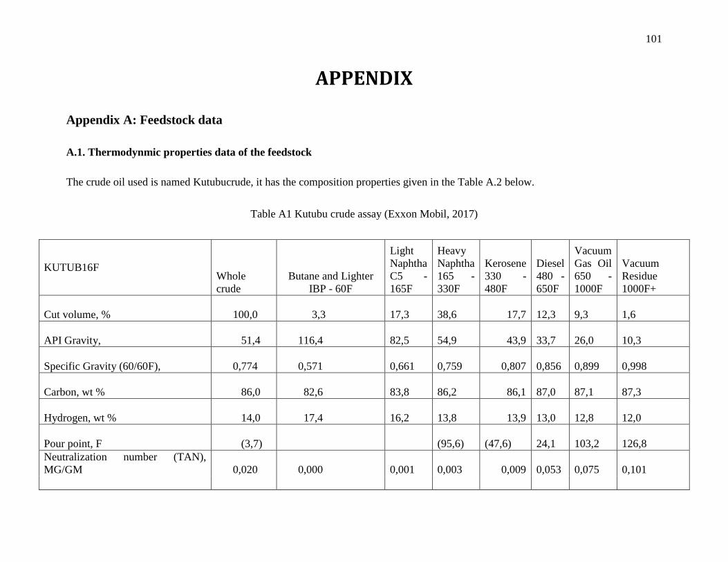
101
APPENDIX
Appendix A: Feedstock data
A.1. Thermodynmic properties data of the feedstock
The crude oil used is named Kutubucrude, it has the composition properties given in the Table A.2 below.
Table A1 Kutubu crude assay (Exxon Mobil, 2017)
KUTUB16F Whole
crude
Butane and Lighter
IBP - 60F
Light
Naphtha
C5 -
165F
Heavy
Naphtha
165 -
330F
Kerosene
330 -
480F
Diesel
480 -
650F
Vacuum
Gas Oil
650 -
1000F
Vacuum
Residue
1000F+
Cut volume, % 100,0 3,3
17,3
38,6 17,7
12,3
9,3
1,6
API Gravity, 51,4 116,4
82,5
54,9 43,9
33,7
26,0
10,3
Specific Gravity (60/60F), 0,774 0,571
0,661
0,759 0,807
0,856
0,899
0,998
Carbon, wt % 86,0 82,6
83,8
86,2 86,1
87,0
87,1
87,3
Hydrogen, wt % 14,0 17,4
16,2
13,8 13,9
13,0
12,8
12,0
Pour point, F (3,7)
(95,6)
(47,6)
24,1
103,2
126,8
Neutralization number (TAN),
MG/GM 0,020 0,000
0,001
0,003 0,009
0,053
0,075
0,101
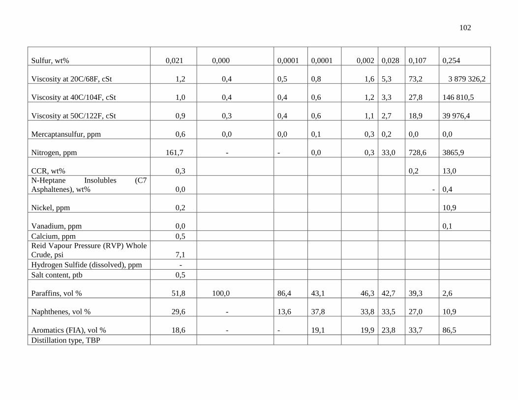
102
Sulfur, wt% 0,021 0,000
0,0001
0,0001 0,002
0,028
0,107
0,254
Viscosity at 20C/68F, cSt 1,2 0,4
0,5
0,8 1,6
5,3
73,2 3 879 326,2
Viscosity at 40C/104F, cSt 1,0 0,4
0,4
0,6 1,2
3,3
27,8 146 810,5
Viscosity at 50C/122F, cSt 0,9 0,3
0,4
0,6 1,1
2,7
18,9 39 976,4
Mercaptansulfur, ppm 0,6 0,0
0,0
0,1 0,3
0,2
0,0
0,0
Nitrogen, ppm 161,7 -
-
0,0 0,3
33,0
728,6 3865,9
CCR, wt% 0,3
0,2
13,0
N-Heptane Insolubles (C7
Asphaltenes), wt% 0,0 -
0,4
Nickel, ppm 0,2
10,9
Vanadium, ppm 0,0
0,1
Calcium, ppm 0,5
Reid Vapour Pressure (RVP) Whole
Crude, psi 7,1
Hydrogen Sulfide (dissolved), ppm -
Salt content, ptb 0,5
Paraffins, vol % 51,8 100,0
86,4
43,1 46,3
42,7
39,3
2,6
Naphthenes, vol % 29,6 -
13,6
37,8 33,8
33,5
27,0
10,9
Aromatics (FIA), vol % 18,6 -
-
19,1 19,9
23,8
33,7
86,5
Distillation type, TBP
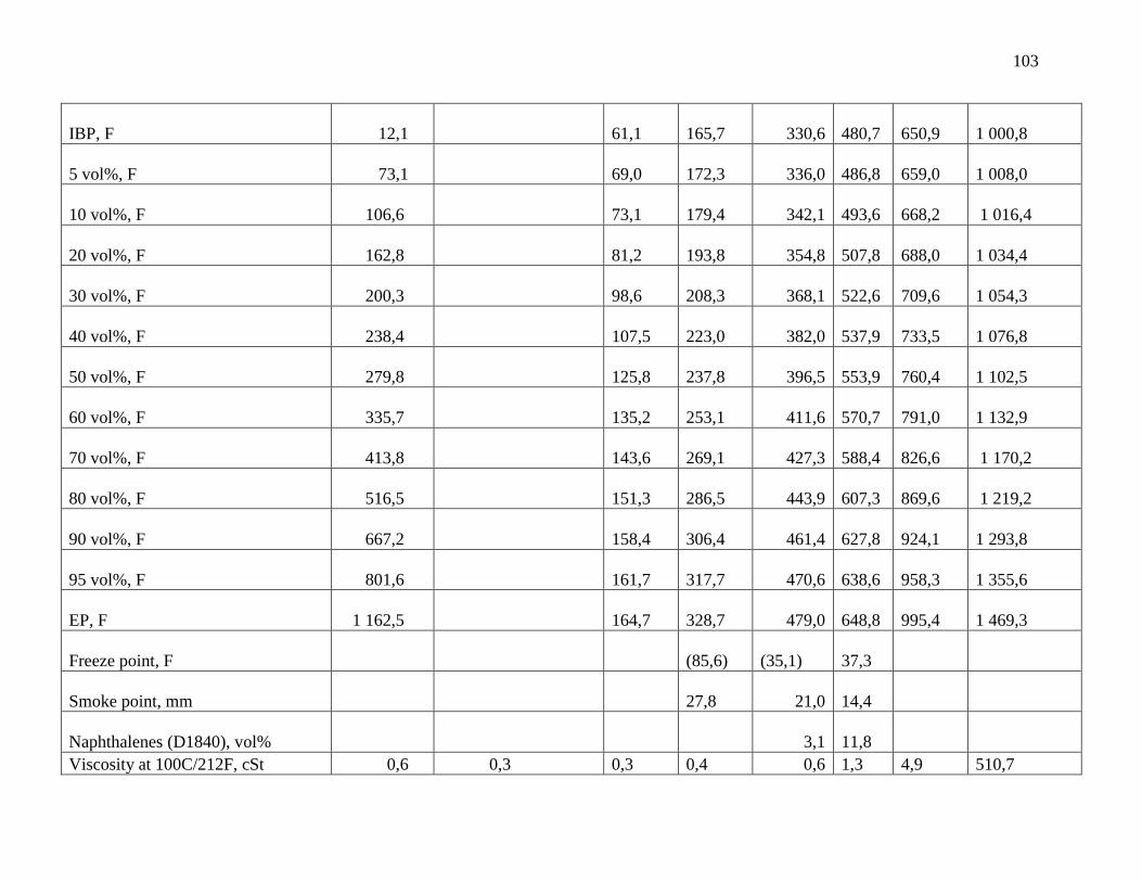
103
IBP, F 12,1
61,1
165,7 330,6
480,7
650,9 1 000,8
5 vol%, F 73,1
69,0
172,3 336,0
486,8
659,0 1 008,0
10 vol%, F 106,6
73,1
179,4 342,1
493,6
668,2 1 016,4
20 vol%, F 162,8
81,2
193,8 354,8
507,8
688,0 1 034,4
30 vol%, F 200,3
98,6
208,3 368,1
522,6
709,6 1 054,3
40 vol%, F 238,4
107,5
223,0 382,0
537,9
733,5 1 076,8
50 vol%, F 279,8
125,8
237,8 396,5
553,9
760,4 1 102,5
60 vol%, F 335,7
135,2
253,1 411,6
570,7
791,0 1 132,9
70 vol%, F 413,8
143,6
269,1 427,3
588,4
826,6 1 170,2
80 vol%, F 516,5
151,3
286,5 443,9
607,3
869,6 1 219,2
90 vol%, F 667,2
158,4
306,4 461,4
627,8
924,1 1 293,8
95 vol%, F 801,6
161,7
317,7 470,6
638,6
958,3 1 355,6
EP, F 1 162,5
164,7
328,7 479,0
648,8
995,4 1 469,3
Freeze point, F
(85,6)
(35,1)
37,3
Smoke point, mm
27,8 21,0
14,4
Naphthalenes (D1840), vol% 3,1
11,8
Viscosity at 100C/212F, cSt 0,6 0,3 0,3 0,4 0,6 1,3 4,9 510,7
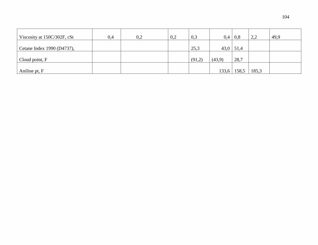
104
Viscosity at 150C/302F, cSt 0,4 0,2
0,2
0,3 0,4
0,8
2,2
49,9
Cetane Index 1990 (D4737),
25,3 43,0
51,4
Cloud point, F
(91,2)
(43,9)
28,7
Aniline pt, F 133,6
158,5
185,3
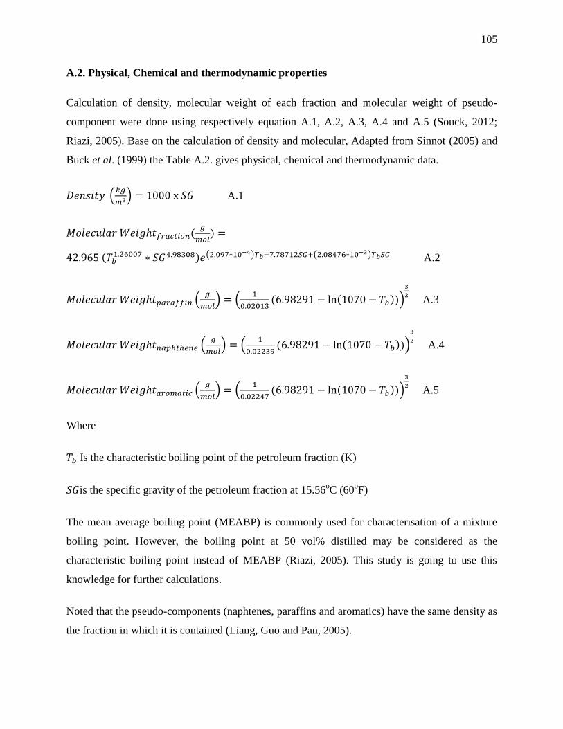
105
A.2. Physical, Chemical and thermodynamic properties
Calculation of density, molecular weight of each fraction and molecular weight of pseudo-
component were done using respectively equation A.1, A.2, A.3, A.4 and A.5 (Souck, 2012;
Riazi, 2005). Base on the calculation of density and molecular, Adapted from Sinnot (2005) and
Buck et al. (1999) the Table A.2. gives physical, chemical and thermodynamic data.
𝐷𝑒𝑛𝑠𝑖𝑡𝑦 (𝑘𝑔
𝑚3) = 1000 x 𝑆𝐺 A.1
𝑀𝑜𝑙𝑒𝑐𝑢𝑙𝑎𝑟 𝑊𝑒𝑖𝑔ℎ𝑡𝑓𝑟𝑎𝑐𝑡𝑖𝑜𝑛(𝑔
𝑚𝑜𝑙) =
42.965 (𝑇𝑏1.26007 ∗ 𝑆𝐺4.98308)𝑒(2.097∗10−4)𝑇𝑏−7.78712𝑆𝐺+(2.08476∗10−3)𝑇𝑏𝑆𝐺 A.2
𝑀𝑜𝑙𝑒𝑐𝑢𝑙𝑎𝑟 𝑊𝑒𝑖𝑔ℎ𝑡𝑝𝑎𝑟𝑎𝑓𝑓𝑖𝑛 (𝑔
𝑚𝑜𝑙) = (
1
0.02013(6.98291 − ln(1070 − 𝑇𝑏)))
3
2 A.3
𝑀𝑜𝑙𝑒𝑐𝑢𝑙𝑎𝑟 𝑊𝑒𝑖𝑔ℎ𝑡𝑛𝑎𝑝ℎ𝑡ℎ𝑒𝑛𝑒 (𝑔
𝑚𝑜𝑙) = (
1
0.02239(6.98291 − ln(1070 − 𝑇𝑏)))
3
2 A.4
𝑀𝑜𝑙𝑒𝑐𝑢𝑙𝑎𝑟 𝑊𝑒𝑖𝑔ℎ𝑡𝑎𝑟𝑜𝑚𝑎𝑡𝑖𝑐 (𝑔
𝑚𝑜𝑙) = (
1
0.02247(6.98291 − ln(1070 − 𝑇𝑏)))
3
2 A.5
Where
𝑇𝑏 Is the characteristic boiling point of the petroleum fraction (K)
𝑆𝐺is the specific gravity of the petroleum fraction at 15.56oC (60
oF)
The mean average boiling point (MEABP) is commonly used for characterisation of a mixture
boiling point. However, the boiling point at 50 vol% distilled may be considered as the
characteristic boiling point instead of MEABP (Riazi, 2005). This study is going to use this
knowledge for further calculations.
Noted that the pseudo-components (naphtenes, paraffins and aromatics) have the same density as
the fraction in which it is contained (Liang, Guo and Pan, 2005).
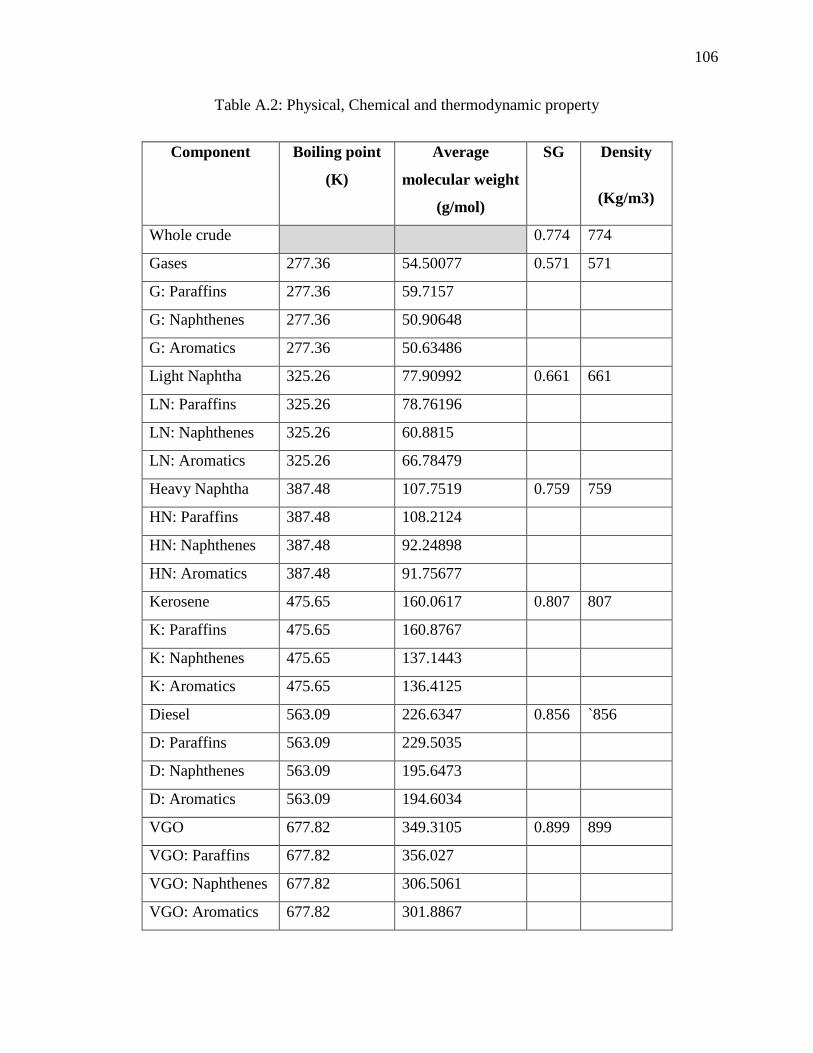
106
Table A.2: Physical, Chemical and thermodynamic property
Component Boiling point
(K)
Average
molecular weight
(g/mol)
SG Density
(Kg/m3)
Whole crude 0.774 774
Gases 277.36 54.50077 0.571 571
G: Paraffins 277.36 59.7157
G: Naphthenes 277.36 50.90648
G: Aromatics 277.36 50.63486
Light Naphtha 325.26 77.90992 0.661 661
LN: Paraffins 325.26 78.76196
LN: Naphthenes 325.26 60.8815
LN: Aromatics 325.26 66.78479
Heavy Naphtha 387.48 107.7519 0.759 759
HN: Paraffins 387.48 108.2124
HN: Naphthenes 387.48 92.24898
HN: Aromatics 387.48 91.75677
Kerosene 475.65 160.0617 0.807 807
K: Paraffins 475.65 160.8767
K: Naphthenes 475.65 137.1443
K: Aromatics 475.65 136.4125
Diesel 563.09 226.6347 0.856 `856
D: Paraffins 563.09 229.5035
D: Naphthenes 563.09 195.6473
D: Aromatics 563.09 194.6034
VGO 677.82 349.3105 0.899 899
VGO: Paraffins 677.82 356.027
VGO: Naphthenes 677.82 306.5061
VGO: Aromatics 677.82 301.8867
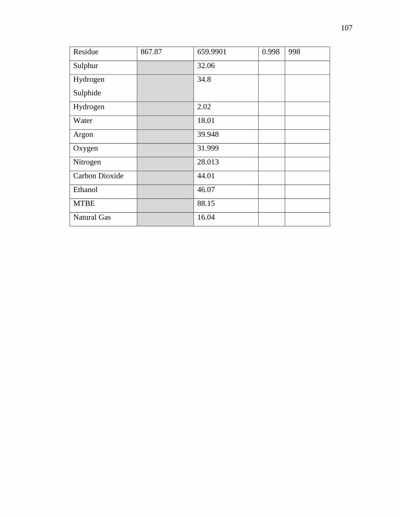
107
Residue 867.87 659.9901 0.998 998
Sulphur 32.06
Hydrogen
Sulphide
34.8
Hydrogen 2.02
Water 18.01
Argon 39.948
Oxygen 31.999
Nitrogen 28.013
Carbon Dioxide 44.01
Ethanol 46.07
MTBE 88.15
Natural Gas 16.04
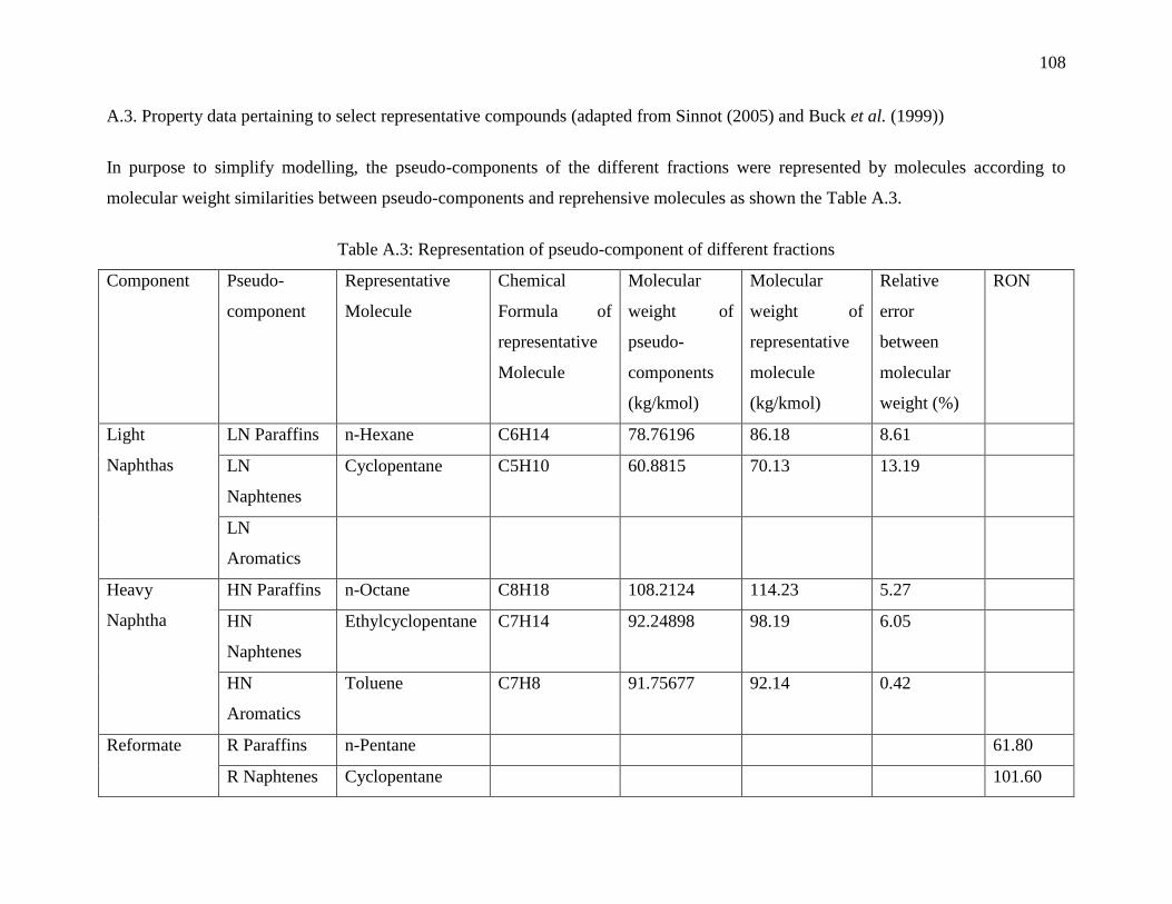
108
A.3. Property data pertaining to select representative compounds (adapted from Sinnot (2005) and Buck et al. (1999))
In purpose to simplify modelling, the pseudo-components of the different fractions were represented by molecules according to
molecular weight similarities between pseudo-components and reprehensive molecules as shown the Table A.3.
Table A.3: Representation of pseudo-component of different fractions
Component Pseudo-
component
Representative
Molecule
Chemical
Formula of
representative
Molecule
Molecular
weight of
pseudo-
components
(kg/kmol)
Molecular
weight of
representative
molecule
(kg/kmol)
Relative
error
between
molecular
weight (%)
RON
Light
Naphthas
LN Paraffins n-Hexane C6H14 78.76196 86.18 8.61
LN
Naphtenes
Cyclopentane C5H10 60.8815 70.13 13.19
LN
Aromatics
Heavy
Naphtha
HN Paraffins n-Octane C8H18 108.2124 114.23 5.27
HN
Naphtenes
Ethylcyclopentane C7H14 92.24898 98.19 6.05
HN
Aromatics
Toluene C7H8 91.75677 92.14 0.42
Reformate R Paraffins n-Pentane 61.80
R Naphtenes Cyclopentane 101.60
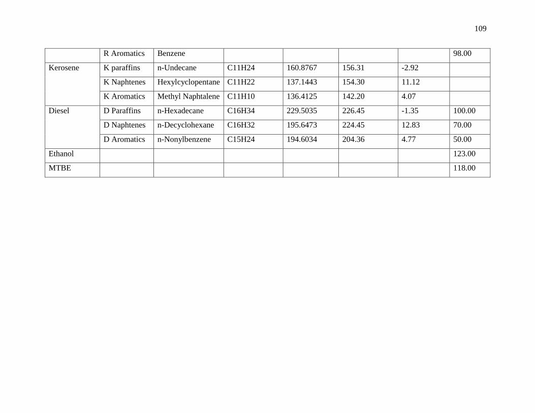
109
R Aromatics Benzene 98.00
Kerosene K paraffins n-Undecane C11H24 160.8767 156.31 -2.92
K Naphtenes Hexylcyclopentane C11H22 137.1443 154.30 11.12
K Aromatics Methyl Naphtalene C11H10 136.4125 142.20 4.07
Diesel D Paraffins n-Hexadecane C16H34 229.5035 226.45 -1.35 100.00
D Naphtenes n-Decyclohexane C16H32 195.6473 224.45 12.83 70.00
D Aromatics n-Nonylbenzene C15H24 194.6034 204.36 4.77 50.00
Ethanol 123.00
MTBE 118.00
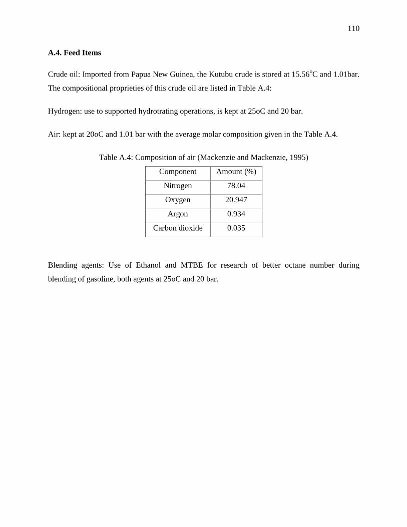
110
A.4. Feed Items
Crude oil: Imported from Papua New Guinea, the Kutubu crude is stored at 15.56oC and 1.01bar.
The compositional proprieties of this crude oil are listed in Table A.4:
Hydrogen: use to supported hydrotrating operations, is kept at 25oC and 20 bar.
Air: kept at 20oC and 1.01 bar with the average molar composition given in the Table A.4.
Table A.4: Composition of air (Mackenzie and Mackenzie, 1995)
Component Amount (%)
Nitrogen 78.04
Oxygen 20.947
Argon 0.934
Carbon dioxide 0.035
Blending agents: Use of Ethanol and MTBE for research of better octane number during
blending of gasoline, both agents at 25oC and 20 bar.
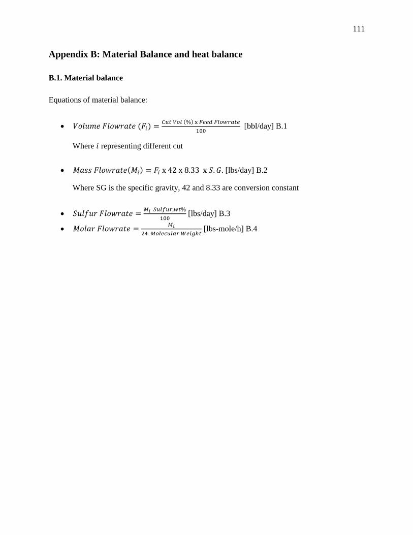
111
Appendix B: Material Balance and heat balance
B.1. Material balance
Equations of material balance:
𝑉𝑜𝑙𝑢𝑚𝑒 𝐹𝑙𝑜𝑤𝑟𝑎𝑡𝑒 (𝐹𝑖) =𝐶𝑢𝑡 𝑉𝑜𝑙 (%) x 𝐹𝑒𝑒𝑑 𝐹𝑙𝑜𝑤𝑟𝑎𝑡𝑒
100 [bbl/day] B.1
Where 𝑖 representing different cut
𝑀𝑎𝑠𝑠 𝐹𝑙𝑜𝑤𝑟𝑎𝑡𝑒(𝑀𝑖) = 𝐹𝑖 x 42 x 8.33 x 𝑆. 𝐺. [lbs/day] B.2
Where SG is the specific gravity, 42 and 8.33 are conversion constant
𝑆𝑢𝑙𝑓𝑢𝑟 𝐹𝑙𝑜𝑤𝑟𝑎𝑡𝑒 =𝑀𝑖 𝑆𝑢𝑙𝑓𝑢𝑟,𝑤𝑡%
100 [lbs/day] B.3
𝑀𝑜𝑙𝑎𝑟 𝐹𝑙𝑜𝑤𝑟𝑎𝑡𝑒 =𝑀𝑖
24 𝑀𝑜𝑙𝑒𝑐𝑢𝑙𝑎𝑟 𝑊𝑒𝑖𝑔ℎ𝑡 [lbs-mole/h] B.4
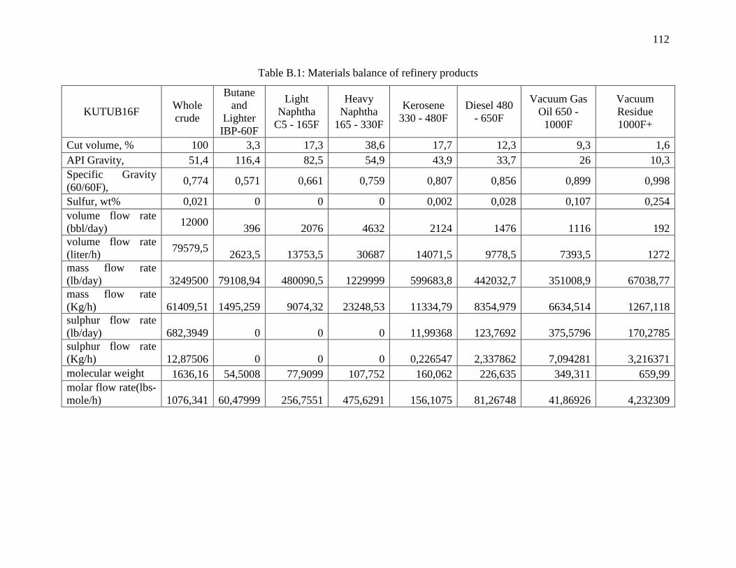
112
Table B.1: Materials balance of refinery products
KUTUB16F Whole
crude
Butane
and
Lighter
IBP-60F
Light
Naphtha
C5 - 165F
Heavy
Naphtha
165 - 330F
Kerosene
330 - 480F
Diesel 480
- 650F
Vacuum Gas
Oil 650 -
1000F
Vacuum
Residue
1000F+
Cut volume, % 100 3,3 17,3 38,6 17,7 12,3 9,3 1,6
API Gravity, 51,4 116,4 82,5 54,9 43,9 33,7 26 10,3
Specific Gravity
(60/60F), 0,774 0,571 0,661 0,759 0,807 0,856 0,899 0,998
Sulfur, wt% 0,021 0 0 0 0,002 0,028 0,107 0,254
volume flow rate
(bbl/day) 12000
396 2076 4632 2124 1476 1116 192
volume flow rate
(liter/h) 79579,5
2623,5 13753,5 30687 14071,5 9778,5 7393,5 1272
mass flow rate
(lb/day) 3249500 79108,94 480090,5 1229999 599683,8 442032,7 351008,9 67038,77
mass flow rate
(Kg/h) 61409,51 1495,259 9074,32 23248,53 11334,79 8354,979 6634,514 1267,118
sulphur flow rate
(lb/day) 682,3949 0 0 0 11,99368 123,7692 375,5796 170,2785
sulphur flow rate
(Kg/h) 12,87506 0 0 0 0,226547 2,337862 7,094281 3,216371
molecular weight 1636,16 54,5008 77,9099 107,752 160,062 226,635 349,311 659,99
molar flow rate(lbs-
mole/h) 1076,341 60,47999 256,7551 475,6291 156,1075 81,26748 41,86926 4,232309
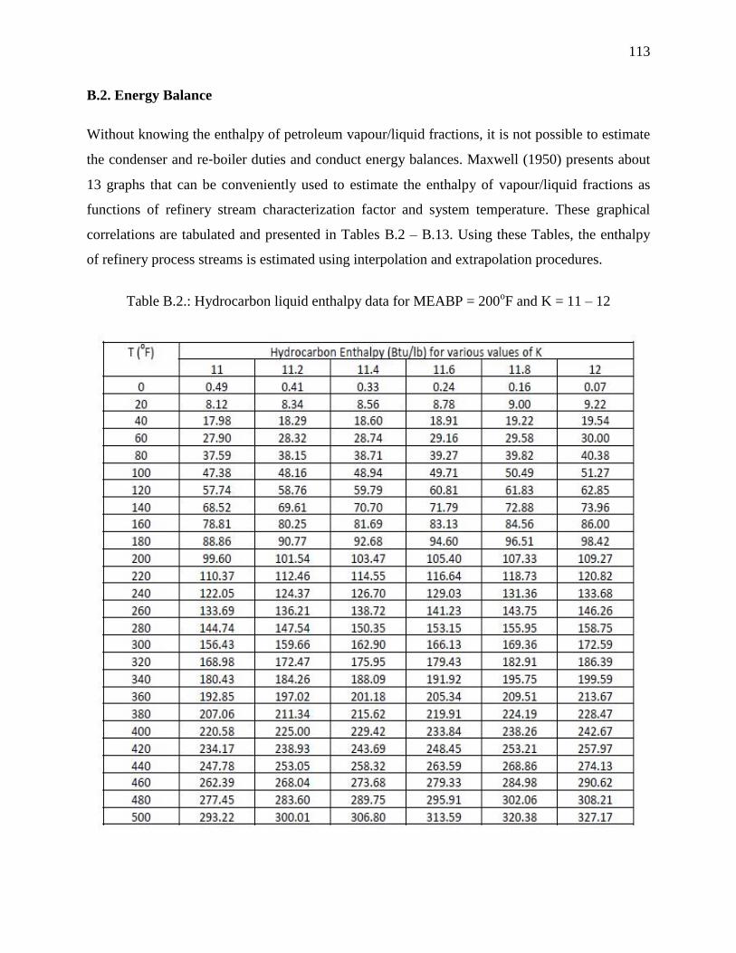
113
B.2. Energy Balance
Without knowing the enthalpy of petroleum vapour/liquid fractions, it is not possible to estimate
the condenser and re‐boiler duties and conduct energy balances. Maxwell (1950) presents about
13 graphs that can be conveniently used to estimate the enthalpy of vapour/liquid fractions as
functions of refinery stream characterization factor and system temperature. These graphical
correlations are tabulated and presented in Tables B.2 – B.13. Using these Tables, the enthalpy
of refinery process streams is estimated using interpolation and extrapolation procedures.
Table B.2.: Hydrocarbon liquid enthalpy data for MEABP = 200oF and K = 11 – 12
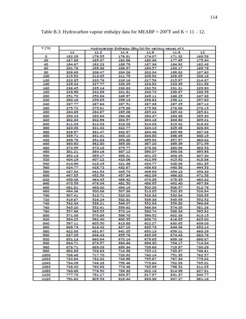
114
Table B.3: Hydrocarbon vapour enthalpy data for MEABP = 200oF and K = 11 – 12.
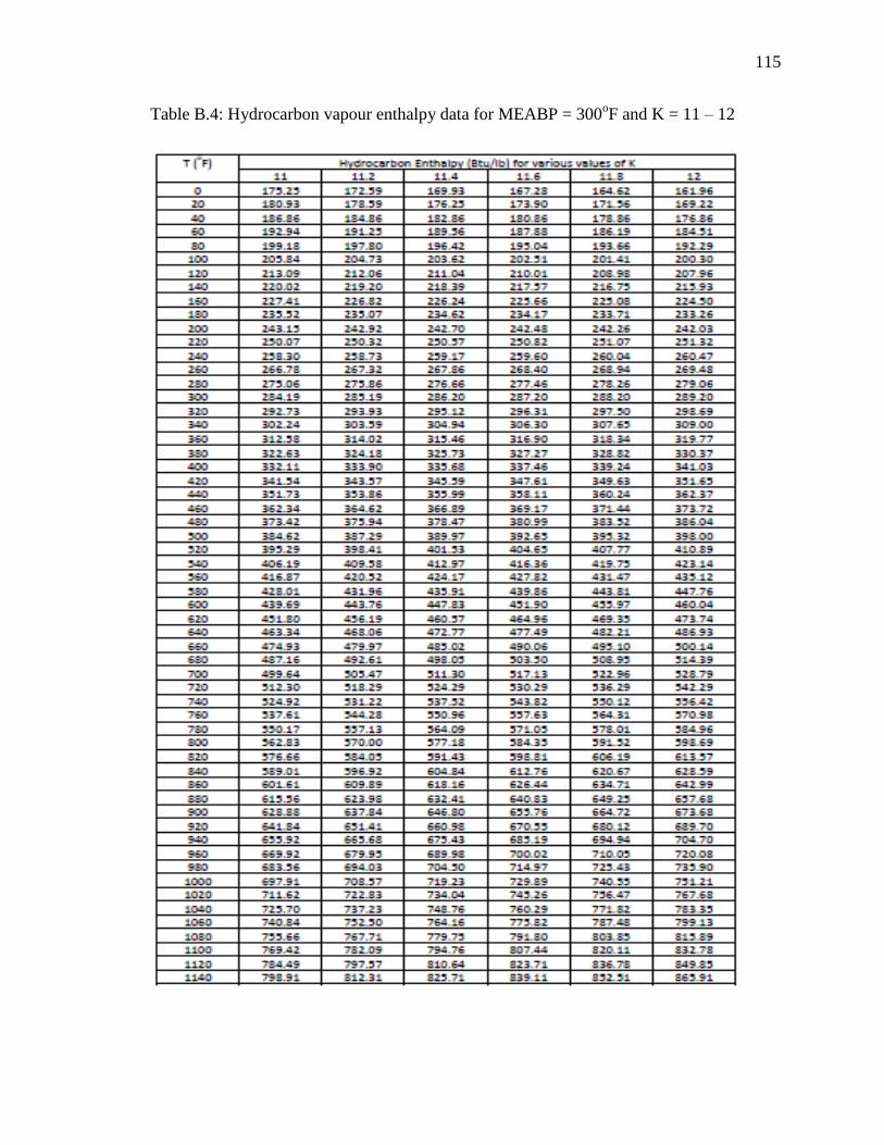
115
Table B.4: Hydrocarbon vapour enthalpy data for MEABP = 300oF and K = 11 – 12
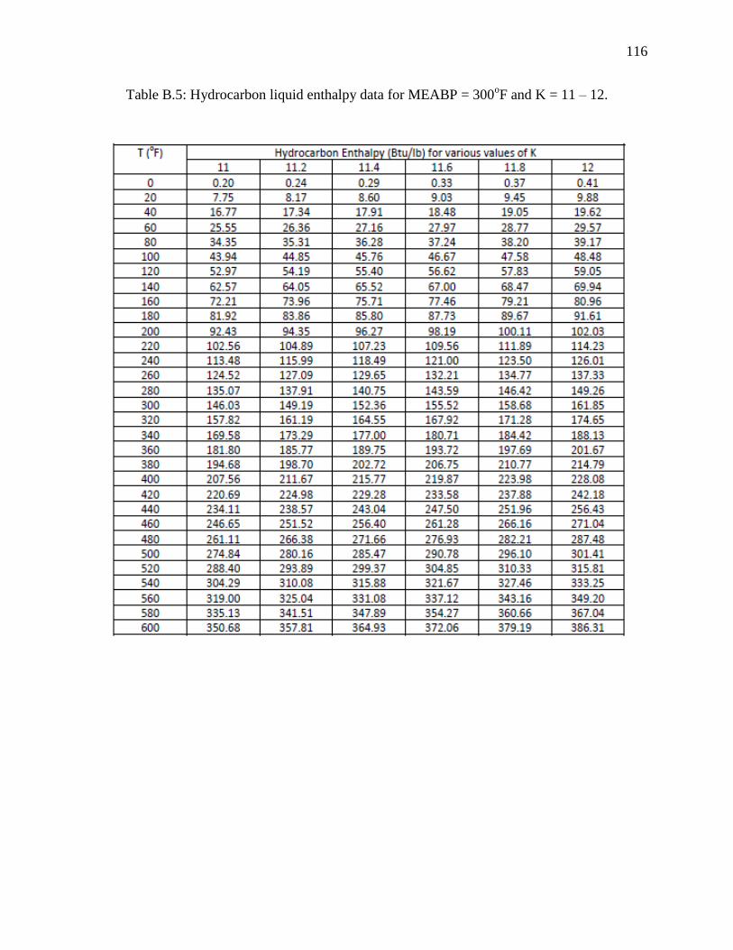
116
Table B.5: Hydrocarbon liquid enthalpy data for MEABP = 300oF and K = 11 – 12.
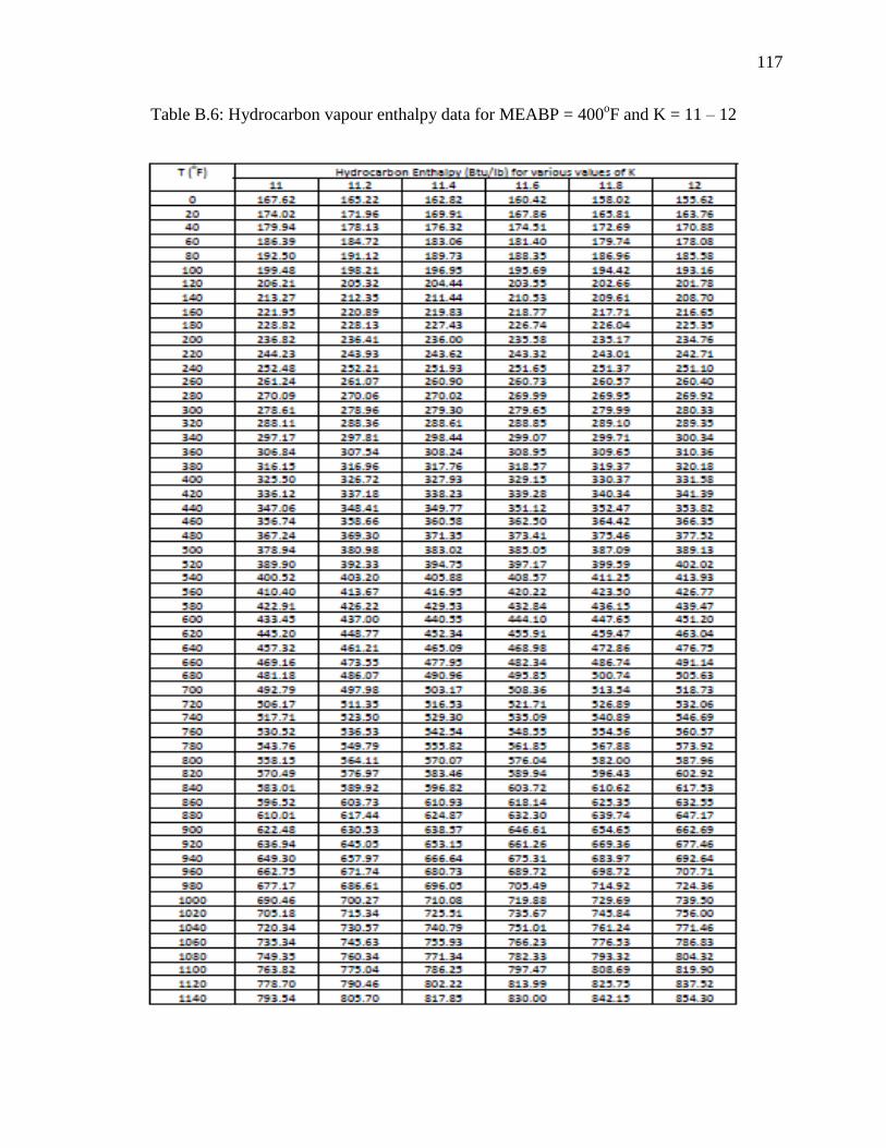
117
Table B.6: Hydrocarbon vapour enthalpy data for MEABP = 400oF and K = 11 – 12
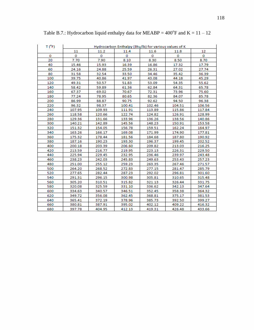
118
Table B.7.: Hydrocarbon liquid enthalpy data for MEABP = 400oF and K = 11 – 12
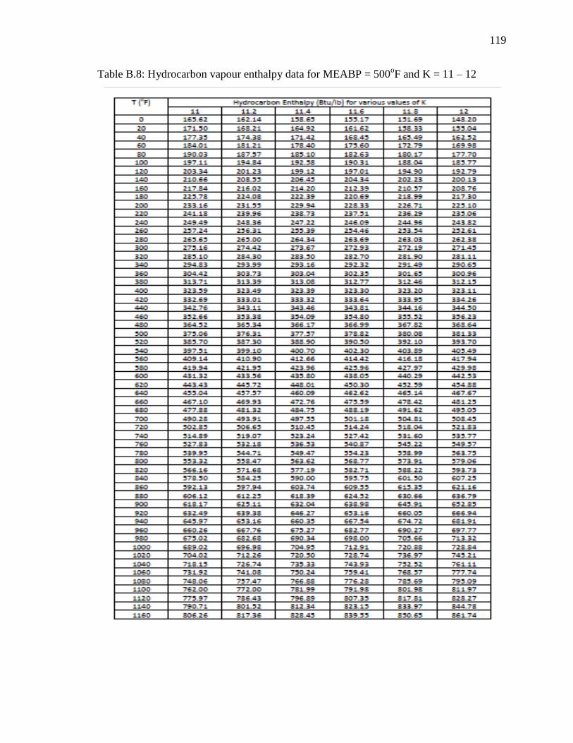
119
Table B.8: Hydrocarbon vapour enthalpy data for MEABP = 500oF and K = 11 – 12
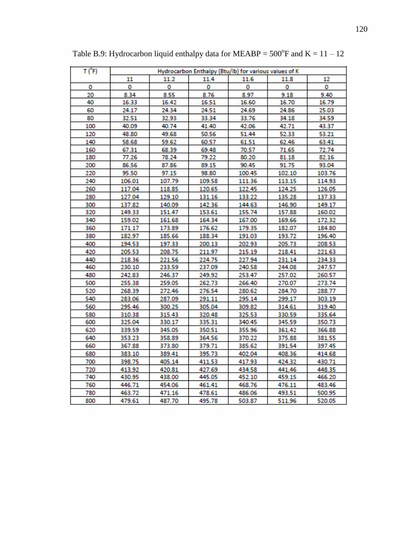
120
Table B.9: Hydrocarbon liquid enthalpy data for MEABP = 500oF and K = 11 – 12
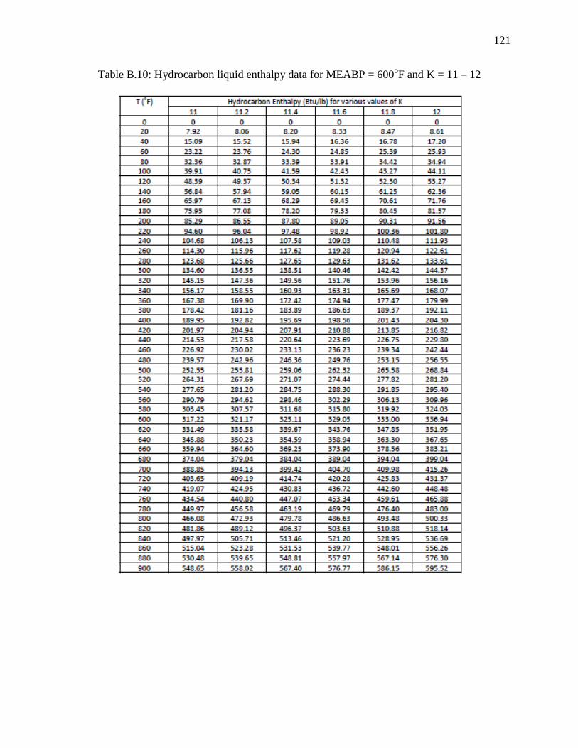
121
Table B.10: Hydrocarbon liquid enthalpy data for MEABP = 600oF and K = 11 – 12
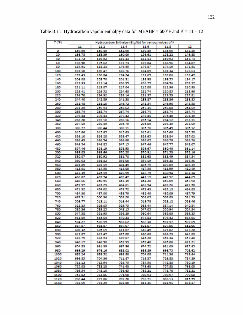
122
Table B.11: Hydrocarbon vapour enthalpy data for MEABP = 600oF and K = 11 – 12
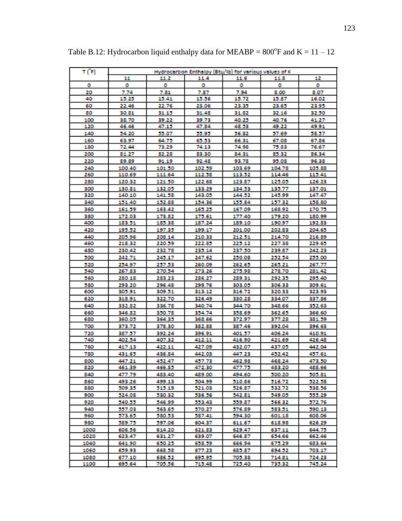
123
Table B.12: Hydrocarbon liquid enthalpy data for MEABP = 800oF and K = 11 – 12
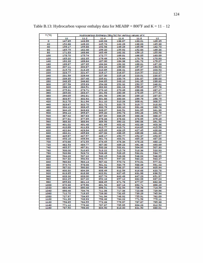
124
Table B.13: Hydrocarbon vapour enthalpy data for MEABP = 800oF and K = 11 – 12
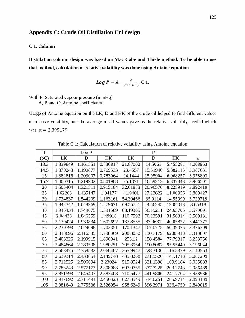
125
Appendix C: Crude Oil Distillation Uni design
C.1. Column
Distillation column design was based on Mac Cabe and Thiele method. To be able to use
that method, calculation of relative volatility was done using Antoine equation.
𝑳𝒐𝒈 𝑷 = 𝑨 −𝑩
𝑪+𝑻 (𝑪𝒐) C.1.
With P: Saturated vapour pressure (mmHg)
A, B and C: Antoine coefficients
Usage of Antoine equation on the LK, D and HK of the crude oil helped to find different values
of relative volatility, and the average of all values gave us the relative volatility needed which
was: α = 2.895179
Table C.1: Calculation of relative volatility using Antoine equation
T
(oC)
Log P P
α LK D HK LK D HK
13.3 1.339849 1.161551 0.736817 21.87002 14.5061 5.455281 4.008963
14.5 1.370248 1.190877 0.769533 23.4557 15.51946 5.882115 3.987631
15 1.382816 1.203007 0.783064 24.1444 15.95904 6.068257 3.978803
15.7 1.400315 1.219902 0.801908 25.1371 16.59212 6.337348 3.966501
20 1.505404 1.321511 0.915184 32.01873 20.96576 8.225919 3.892419
25 1.62263 1.435147 1.04177 41.9401 27.23622 11.00956 3.809427
30 1.734837 1.544209 1.163161 54.30466 35.0114 14.55999 3.729719
35 1.842342 1.648969 1.279671 69.55721 44.56245 19.04018 3.65318
40 1.945434 1.749675 1.391589 88.19305 56.19211 24.63705 3.579691
45 2.04438 1.846559 1.49918 110.7592 70.23591 31.56314 3.509131
50 2.139424 1.939834 1.602692 137.8555 87.0631 40.05822 3.441377
55 2.230793 2.029698 1.702351 170.1347 107.0775 50.39075 3.376309
60 2.318696 2.116335 1.798369 208.3032 130.7179 62.85918 3.313807
65 2.403326 2.199915 1.890941 253.12 158.4584 77.79317 3.253756
70 2.484864 2.280598 1.980251 305.3964 190.8087 95.55449 3.196044
75 2.563475 2.358532 2.066467 365.9947 228.3136 116.5379 3.140563
80 2.639314 2.433854 2.149748 435.8268 271.5526 141.1718 3.087209
85 2.712525 2.506694 2.23024 515.8524 321.1398 169.9184 3.035883
90 2.783243 2.577173 2.308083 607.0765 377.7225 203.2743 2.986489
95 2.851593 2.645403 2.383403 710.5477 441.9806 241.7704 2.938936
100 2.917692 2.711491 2.456323 827.3549 514.6251 285.9714 2.893139
105 2.981649 2.775536 2.526954 958.6249 596.3971 336.4759 2.849015
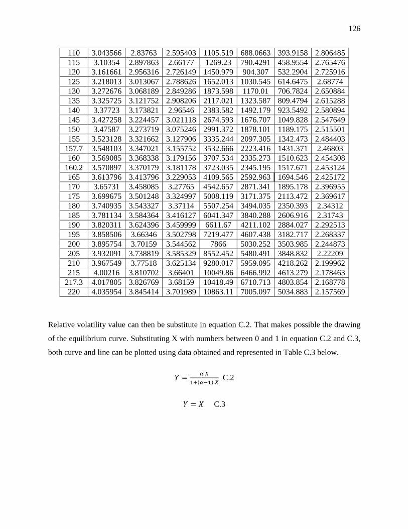
126
110 3.043566 2.83763 2.595403 1105.519 688.0663 393.9158 2.806485
115 3.10354 2.897863 2.66177 1269.23 790.4291 458.9554 2.765476
120 3.161661 2.956316 2.726149 1450.979 904.307 532.2904 2.725916
125 3.218013 3.013067 2.788626 1652.013 1030.545 614.6475 2.68774
130 3.272676 3.068189 2.849286 1873.598 1170.01 706.7824 2.650884
135 3.325725 3.121752 2.908206 2117.021 1323.587 809.4794 2.615288
140 3.37723 3.173821 2.96546 2383.582 1492.179 923.5492 2.580894
145 3.427258 3.224457 3.021118 2674.593 1676.707 1049.828 2.547649
150 3.47587 3.273719 3.075246 2991.372 1878.101 1189.175 2.515501
155 3.523128 3.321662 3.127906 3335.244 2097.305 1342.473 2.484403
157.7 3.548103 3.347021 3.155752 3532.666 2223.416 1431.371 2.46803
160 3.569085 3.368338 3.179156 3707.534 2335.273 1510.623 2.454308
160.2 3.570897 3.370179 3.181178 3723.035 2345.195 1517.671 2.453124
165 3.613796 3.413796 3.229053 4109.565 2592.963 1694.546 2.425172
170 3.65731 3.458085 3.27765 4542.657 2871.341 1895.178 2.396955
175 3.699675 3.501248 3.324997 5008.119 3171.375 2113.472 2.369617
180 3.740935 3.543327 3.37114 5507.254 3494.035 2350.393 2.34312
185 3.781134 3.584364 3.416127 6041.347 3840.288 2606.916 2.31743
190 3.820311 3.624396 3.459999 6611.67 4211.102 2884.027 2.292513
195 3.858506 3.66346 3.502798 7219.477 4607.438 3182.717 2.268337
200 3.895754 3.70159 3.544562 7866 5030.252 3503.985 2.244873
205 3.932091 3.738819 3.585329 8552.452 5480.491 3848.832 2.22209
210 3.967549 3.77518 3.625134 9280.017 5959.095 4218.262 2.199962
215 4.00216 3.810702 3.66401 10049.86 6466.992 4613.279 2.178463
217.3 4.017805 3.826769 3.68159 10418.49 6710.713 4803.854 2.168778
220 4.035954 3.845414 3.701989 10863.11 7005.097 5034.883 2.157569
Relative volatility value can then be substitute in equation C.2. That makes possible the drawing
of the equilibrium curve. Substituting X with numbers between 0 and 1 in equation C.2 and C.3,
both curve and line can be plotted using data obtained and represented in Table C.3 below.
𝑌 =𝛼 𝑋
1+(𝛼−1) 𝑋 C.2
𝑌 = 𝑋 C.3
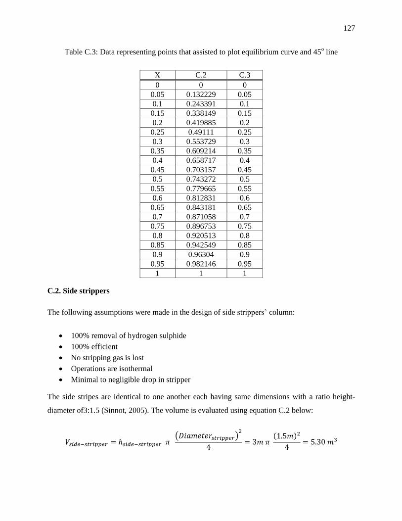
127
Table C.3: Data representing points that assisted to plot equilibrium curve and 45o line
X C.2 C.3
0 0 0
0.05 0.132229 0.05
0.1 0.243391 0.1
0.15 0.338149 0.15
0.2 0.419885 0.2
0.25 0.49111 0.25
0.3 0.553729 0.3
0.35 0.609214 0.35
0.4 0.658717 0.4
0.45 0.703157 0.45
0.5 0.743272 0.5
0.55 0.779665 0.55
0.6 0.812831 0.6
0.65 0.843181 0.65
0.7 0.871058 0.7
0.75 0.896753 0.75
0.8 0.920513 0.8
0.85 0.942549 0.85
0.9 0.96304 0.9
0.95 0.982146 0.95
1 1 1
C.2. Side strippers
The following assumptions were made in the design of side strippers’ column:
100% removal of hydrogen sulphide
100% efficient
No stripping gas is lost
Operations are isothermal
Minimal to negligible drop in stripper
The side stripes are identical to one another each having same dimensions with a ratio height-
diameter of3:1.5 (Sinnot, 2005). The volume is evaluated using equation C.2 below:
𝑉𝑠𝑖𝑑𝑒−𝑠𝑡𝑟𝑖𝑝𝑝𝑒𝑟 = ℎ𝑠𝑖𝑑𝑒−𝑠𝑡𝑟𝑖𝑝𝑝𝑒𝑟 𝜋 (𝐷𝑖𝑎𝑚𝑒𝑡𝑒𝑟𝑠𝑡𝑟𝑖𝑝𝑝𝑒𝑟)
2
4= 3𝑚 𝜋
(1.5𝑚)2
4= 5.30 𝑚3
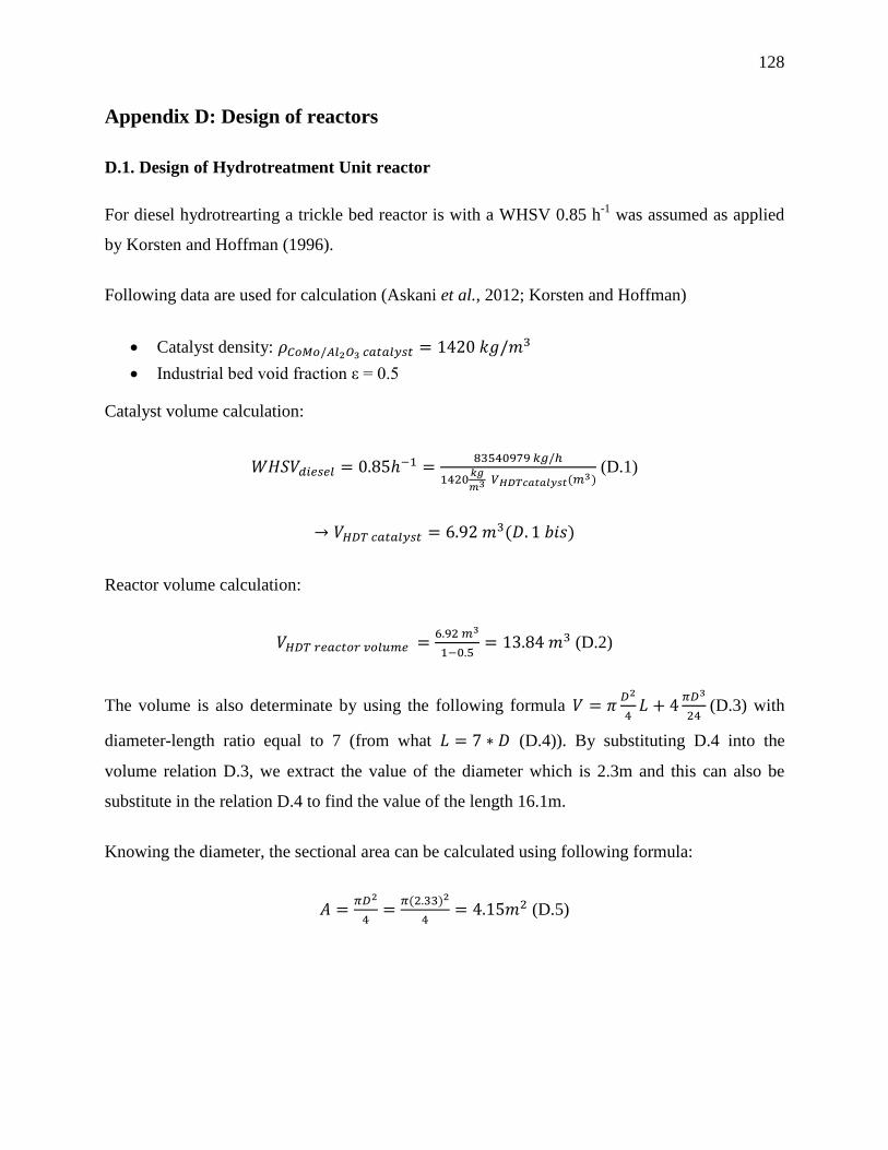
128
Appendix D: Design of reactors
D.1. Design of Hydrotreatment Unit reactor
For diesel hydrotrearting a trickle bed reactor is with a WHSV 0.85 h-1
was assumed as applied
by Korsten and Hoffman (1996).
Following data are used for calculation (Askani et al., 2012; Korsten and Hoffman)
Catalyst density: 𝜌𝐶𝑜𝑀𝑜/𝐴𝑙2𝑂3 𝑐𝑎𝑡𝑎𝑙𝑦𝑠𝑡 = 1420 𝑘𝑔/𝑚3
Industrial bed void fraction ε = 0.5
Catalyst volume calculation:
𝑊𝐻𝑆𝑉𝑑𝑖𝑒𝑠𝑒𝑙 = 0.85ℎ−1 =83540979 𝑘𝑔/ℎ
1420𝑘𝑔
𝑚3 𝑉𝐻𝐷𝑇𝑐𝑎𝑡𝑎𝑙𝑦𝑠𝑡(𝑚3) (D.1)
→ 𝑉𝐻𝐷𝑇 𝑐𝑎𝑡𝑎𝑙𝑦𝑠𝑡 = 6.92 𝑚3(𝐷. 1 𝑏𝑖𝑠)
Reactor volume calculation:
𝑉𝐻𝐷𝑇 𝑟𝑒𝑎𝑐𝑡𝑜𝑟 𝑣𝑜𝑙𝑢𝑚𝑒 =6.92 𝑚3
1−0.5= 13.84 𝑚3 (D.2)
The volume is also determinate by using the following formula 𝑉 = 𝜋𝐷2
4𝐿 + 4
𝜋𝐷3
24 (D.3) with
diameter-length ratio equal to 7 (from what 𝐿 = 7 ∗ 𝐷 (D.4)). By substituting D.4 into the
volume relation D.3, we extract the value of the diameter which is 2.3m and this can also be
substitute in the relation D.4 to find the value of the length 16.1m.
Knowing the diameter, the sectional area can be calculated using following formula:
𝐴 =𝜋𝐷2
4=
𝜋(2.33)2
4= 4.15𝑚2 (D.5)
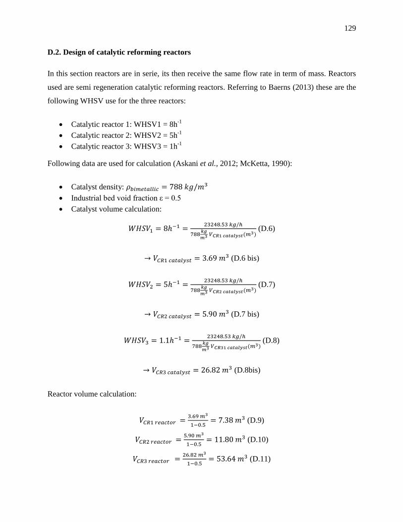
129
D.2. Design of catalytic reforming reactors
In this section reactors are in serie, its then receive the same flow rate in term of mass. Reactors
used are semi regeneration catalytic reforming reactors. Referring to Baerns (2013) these are the
following WHSV use for the three reactors:
Catalytic reactor 1: WHSV1 = 8h-1
Catalytic reactor 2: WHSV2 = 5h-1
Catalytic reactor 3: WHSV3 = 1h-1
Following data are used for calculation (Askani et al., 2012; McKetta, 1990):
Catalyst density: 𝜌𝑏𝑖𝑚𝑒𝑡𝑎𝑙𝑙𝑖𝑐 = 788 𝑘𝑔/𝑚3
Industrial bed void fraction ε = 0.5
Catalyst volume calculation:
𝑊𝐻𝑆𝑉1 = 8ℎ−1 =23248.53 𝑘𝑔/ℎ
788𝑘𝑔
𝑚3 𝑉𝐶𝑅1 𝑐𝑎𝑡𝑎𝑙𝑦𝑠𝑡(𝑚3) (D.6)
→ 𝑉𝐶𝑅1 𝑐𝑎𝑡𝑎𝑙𝑦𝑠𝑡 = 3.69 𝑚3 (D.6 bis)
𝑊𝐻𝑆𝑉2 = 5ℎ−1 =23248.53 𝑘𝑔/ℎ
788𝑘𝑔
𝑚3 𝑉𝐶𝑅2 𝑐𝑎𝑡𝑎𝑙𝑦𝑠𝑡(𝑚3) (D.7)
→ 𝑉𝐶𝑅2 𝑐𝑎𝑡𝑎𝑙𝑦𝑠𝑡 = 5.90 𝑚3 (D.7 bis)
𝑊𝐻𝑆𝑉3 = 1.1ℎ−1 =23248.53 𝑘𝑔/ℎ
788𝑘𝑔
𝑚3 𝑉𝐶𝑅31 𝑐𝑎𝑡𝑎𝑙𝑦𝑠𝑡(𝑚3) (D.8)
→ 𝑉𝐶𝑅3 𝑐𝑎𝑡𝑎𝑙𝑦𝑠𝑡 = 26.82 𝑚3 (D.8bis)
Reactor volume calculation:
𝑉𝐶𝑅1 𝑟𝑒𝑎𝑐𝑡𝑜𝑟 =3.69 𝑚3
1−0.5= 7.38 𝑚3 (D.9)
𝑉𝐶𝑅2 𝑟𝑒𝑎𝑐𝑡𝑜𝑟 =5.90 𝑚3
1−0.5= 11.80 𝑚3 (D.10)
𝑉𝐶𝑅3 𝑟𝑒𝑎𝑐𝑡𝑜𝑟 =26.82 𝑚3
1−0.5= 53.64 𝑚3 (D.11)