Embed Size (px)
Citation preview
DOCTORA L T H E S I S
Luleå University of TechnologyDepartment of Applied Physics and Mechanical Engineering
Division of Solid Mechanics
2006:30|: 02-5|: - -- 06 ⁄30 --
2006:30
Modelling and Simulation of Hot Stamping
Paul Åkerström

Modelling and Simulation of Hot Stamping
Paul Akerstrom
Division of Solid MechanicsDepartment of Applied Physics and Mechanical Engineering
Lulea University of TechnologySE-97187 Lulea, Sweden
Doctoral thesis
Doctoral Thesis: 2006:30ISSN: 1402-1544ISRN: LTU - DT – 06/30 – SE


To my four girls

PREFACE
This work has been carried out at the Division of Solid Mechanics, Depart-ment of Applied Physics and Mechanical Engineering at Lulea University ofTechnology in Sweden.
Firstly, I would like thank my two supervisors, Professor Mats Oldenburgand Dr. Greger Bergman for their great support and guidance during the courseof this work. Further, a warm thank to Assistant Professor Bengt Wikman andKjell Eriksson for invaluable support and guidance. All colleagues and friendsat the division are given my greatest gratitude.
Secondly, I would like to express my appreciation to friends and colleaguesat Gestamp HardTech which made this project possible. The personnel at theResearch Council of Norrbotten is gratefully acknowledged, especially An-ders Nilsson for a truly fine cooperation. I am also very thankful to MaheshSomani and Pentti Karjalainen, University of Oulu, for performing the Gleebletests used in Paper A and B. Thank you Per Johansson Gestamp HardTech forhelp performing the experiments in paper C and E. Further, thank you JacekKomenda, Swedish Institute for Metals Research for a fine cooperation.
Naturally, my most profound appreciation is directed to my lovely wife Annaand my girls Evelina, Amanda and Ida.
Paul AkerstromLulea, June 2006


ABSTRACT
The growing effort to reduce vehicle weight and improve passive safety inthe automotive industry has drastically increased the demand for ultra highstrength steel components. There are several production technologies for suchcomponents. The hot stamping technology (press hardening) is one of themost successful in producing complex components with superior mechani-cal properties. The hot stamping process can be described by the followingsteps; punching of blanks, heating to 900◦C in a furnace to austenitizationfollowed by simultaneous forming and quenching in forming tools. In or-der to obtain accurate numerical Finite Element (FE) simulations of the actualthermo-mechanical forming, correct material data and models are crucial andmandatory.
This work is focusing on three main aspects, which are described below,for the numerical simulation of the thermo-mechanical forming of thin boronsteel sheets into ultra high strength components. The objective is to predictthe shape accuracy, thickness distribution and hardness distribution of the finalcomponent with high accuracy.
The first aspect is the flow stress of the austenite at elevated temperaturesand different strain rates, which is crucial for correctly predicting the strainsin the component and the forming force. During a hot stamping cycle, theactual forming is performed at high temperatures and the steel is mainly in theaustenitic state. The second aspect is the austenite decomposition into daughterproducts such as ferrite, pearlite, bainite or martensite that is a function of thethermal and mechanical history. The third aspect is the mechanical materialmodel used, which determines the stress state and consequently the componentdistortion.
To find the mechanical response (flow stress) for the austenite, a methodbased on multiple overlapping continuous cooling and compression experi-ments (MOCCCT) in combination with inverse modelling has been devel-oped. A validation test (in combination with the compression tests) showsgood agreement with the simulated forming force, indicating that the estimatedflow stress as a function of temperature, strain and strain rate is accurate in theactual application.
The austenite decomposition model is implemented as a material subroutineinto the FE-code LS-DYNA. The model is based on the combined nucleationand growth rate equations proposed by Kirkaldy. A separate test to obtaindifferent cooling histories along a boron steel sheet has been conducted. Dif-ferent mixtures of daughter products are formed along the sheet and the cor-responding simulation shows acceptable agreement with the experimentally

determined temperature histories, hardness profile and volume fractions of thedifferent microconstituents formed in the process.
For the mechanical response, a mechanical constitutive model based on theoriginal model proposed by Leblond has been implemented into LS-DYNA.The implemented model accounts for transformation induced plasticity (localplastic flow in the austenite) according to the Greenwood-Johnson mechanismas well as classical plasticity during global yield. Finally, a thermo-mechanicalFE-simulation using the implemented models is compared to the correspond-ing experiment. The comparison includes the following; forming force, thick-ness distribution, hardness distribution and shape accuracy/springback.

THESIS
This thesis consists of a survey and the following five appended papers:
Paper A P. Akerstrom and M. Oldenburg. Studies of the thermo-mechanicalmaterial response of a boron steel by inverse modelling. J. Phys. IV120:625-633, 2004.
Paper B P. Akerstrom, B. Wikman and M. Oldenburg. Material parameter es-timation for boron steel from simultaneous cooling and compressionexperiments. Modelling Simul. Mater. Sci. Eng. 13:1291-1308,2005.
Paper C P. Akerstrom and M. Oldenburg. Austenite decomposition duringpress hardening of a boron steel - computer simulation and test, Jour-nal of Materials Processing Technology 174:399-406, 2006.
Paper D P. Akerstrom, G. Bergman and M. Oldenburg. Numerical imple-mentation of a constitutive model for simulation of hot stamping.Submitted for publication.
Paper E P. Akerstrom and M. Oldenburg. Numerical simulation of a thermo-mechanical sheet metal forming experiment. To be submitted.


Contents
1 INTRODUCTION . . . . . . . . . . . . . . . . . . . . . . . . . . . . . . . . . . . . . . . . . . . . . . . . . . . . . . . 11.1 Outline . . . . . . . . . . . . . . . . . . . . . . . . . . . . . 11.2 Background . . . . . . . . . . . . . . . . . . . . . . . . . . . 11.3 Classification of automotive steels . . . . . . . . . . . . . . . 21.4 Ultra high strength components in car body . . . . . . . . . . 41.5 Hot stamping . . . . . . . . . . . . . . . . . . . . . . . . . . 51.6 Objective and Scope . . . . . . . . . . . . . . . . . . . . . . 6
2 MODELLING OF HOT STAMPING .. . . . . . . . . . . . . . . . . . . . . . . . . . . . . . . . 62.1 Mechanical material modelling . . . . . . . . . . . . . . . . . 6
2.1.1 Constitutive modelling . . . . . . . . . . . . . . . . . 82.1.2 Transformation induced plasticity . . . . . . . . . . . 11
2.2 Strain rate effects . . . . . . . . . . . . . . . . . . . . . . . . 132.3 Thermal modelling . . . . . . . . . . . . . . . . . . . . . . . 14
2.3.1 Heat equation . . . . . . . . . . . . . . . . . . . . . . 142.3.2 Boundary conditions - heat transfer . . . . . . . . . . 152.3.3 Thermal shell element . . . . . . . . . . . . . . . . . 18
2.4 Phase transformation modelling . . . . . . . . . . . . . . . . 182.4.1 Diffusional controlled transformations . . . . . . . . . 192.4.2 Diffusionless transformation . . . . . . . . . . . . . . 212.4.3 Effect of stress and strain on phase transformations . . 222.4.4 Latent heat and change in thermal properties . . . . . 23
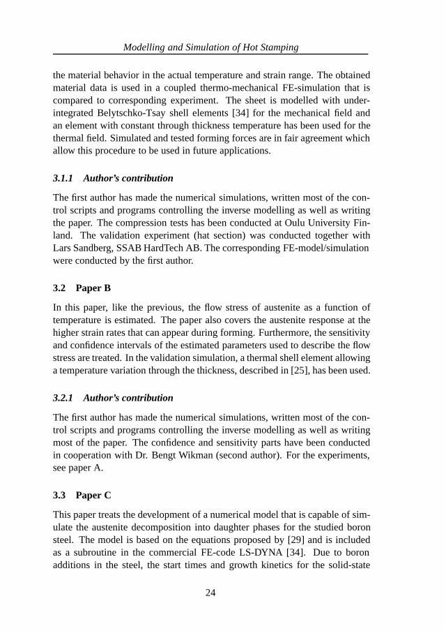
3 SUMMARY OF APPENDED PAPERS . . . . . . . . . . . . . . . . . . . . . . . . . . . . . . . 233.1 Paper A . . . . . . . . . . . . . . . . . . . . . . . . . . . . . 23
3.1.1 Author’s contribution . . . . . . . . . . . . . . . . . . 243.2 Paper B . . . . . . . . . . . . . . . . . . . . . . . . . . . . . 24
3.2.1 Author’s contribution . . . . . . . . . . . . . . . . . . 243.3 Paper C . . . . . . . . . . . . . . . . . . . . . . . . . . . . . 24
3.3.1 Author’s contribution . . . . . . . . . . . . . . . . . . 253.4 Paper D . . . . . . . . . . . . . . . . . . . . . . . . . . . . . 25
3.4.1 Author’s contribution . . . . . . . . . . . . . . . . . . 253.5 Paper E . . . . . . . . . . . . . . . . . . . . . . . . . . . . . 26
3.5.1 Author’s contribution . . . . . . . . . . . . . . . . . . 26
4 DISCUSSION AND CONCLUSIONS .. . . . . . . . . . . . . . . . . . . . . . . . . . . . . . . . 26
5 SUGGESTIONS FOR FUTURE WORK .. . . . . . . . . . . . . . . . . . . . . . . . . . . . 27

REFERENCES .. . . . . . . . . . . . . . . . . . . . . . . . . . . . . . . . . . . . . . . . . . . . . . . . . . . . . . . . . . . . . . 28
APPENDED PAPERS
A Studies of the thermo-mechanical material response of a boron steel by in-verse modelling.
B Material parameter estimation for boron steel from simultaneous coolingand compression experiments.
C Austenite decomposition during press hardening of a boron steel - computersimulation and test.
D Numerical implementation of a constitutive model for simulation of hotstamping.
E Numerical simulation of a thermo-mechanical sheet metal forming experi-ment.

Paul Akerstrom
1 INTRODUCTION
1.1 Outline
The thesis consists of an introductory survey and five appended papers. Theintroduction gives an insight into the hot stamping technique and the objectivesof the work, followed by an introduction to the modelling and simulation ofhot stamping with some results. Finally, a description of the appended papers,conclusions and suggestions for future work follow.
1.2 Background
Due to continuously higher demands from different organizations and severelegislation on passive automotive safety and the effort to reduce vehicle emis-sions, the use of high- and ultra high strength components in both car bodyand closures have increased drastically during the last two decades. Manytypes and classes of materials, both metallic and nonmetallic are used. Re-garding metallic materials, aluminium alloys and different steel grades are themost common in car body components and reinforcement beams. Simultane-ous forming and quenching is a current manufacturing process for low weightand ultra high strength components. The process is often referred to as hotstamping or press hardening and is mainly used for producing passive safetycomponents such as side impact beams, bumper beams and different types ofreinforcement components. Conventional cold forming of high strength steelis often limited to the production of relatively simple geometries, due to lim-ited formability. During cold forming operations, high forming forces, largespringback and excessive tool wear often arise as a consequence. Alterna-tively, it is possible to use a hardenable steel, forming it in the hot state, fol-lowed by fixing and hardening. If the cold formed component is hardenedwithout fixing in a special tool, excessive distortion often arise and straight-ening is necessary. Such additional operations are expensive and generallynot economically profitable for large series. The hot stamping is a techniquethat avoids many of these disadvantages and additional forming steps, and willshortly be described in section 1.5. In the design of new products and cor-responding tools, considerable costs often arises from the traditional productdevelopment process. This process often include prototype manufacturing andtests, if the product fails to fulfil the functional requirements, it is re-designed.With numerical simulations in the design stage, the efficiency of the productdevelopment can be strongly improved, leading to a reduction in lead time andcosts. Numerical methods such as the finite element (FE) method, see e.g.
1
Modelling and Simulation of Hot Stamping
[1, 2, 3, 4], is often employed in simulations of manufacturing processes andcomponent functionality.
1.3 Classification of automotive steels
Automotive steels can be defined in several different ways. The list belowsummarizes these definitions according to [5].
1. By metallurgical designation
- Low-strength steels: interstitial-free (IF) and mild steels
- Conventional high-strength steels: carbon-manganese(CMn), bakehardenable (BH), interstitial free high-strength (IF-HS) and highstrength low-alloy steels (HSLA)
- Advanced-high-strength steels (AHSS): dual phase (DP), transfor-mation induced plasticity (TRIP), complex phase (CP) and marten-sitic steels
2. Mechanical properties - tensile strength
- Low-strength steels, LSS: tensile strength < 270 MPa
- High-strength steels, HSS1: tensile strength 270 - 700 MPa
- Ultra-high-strength steels, UHSS: tensile strength > 700 MPa
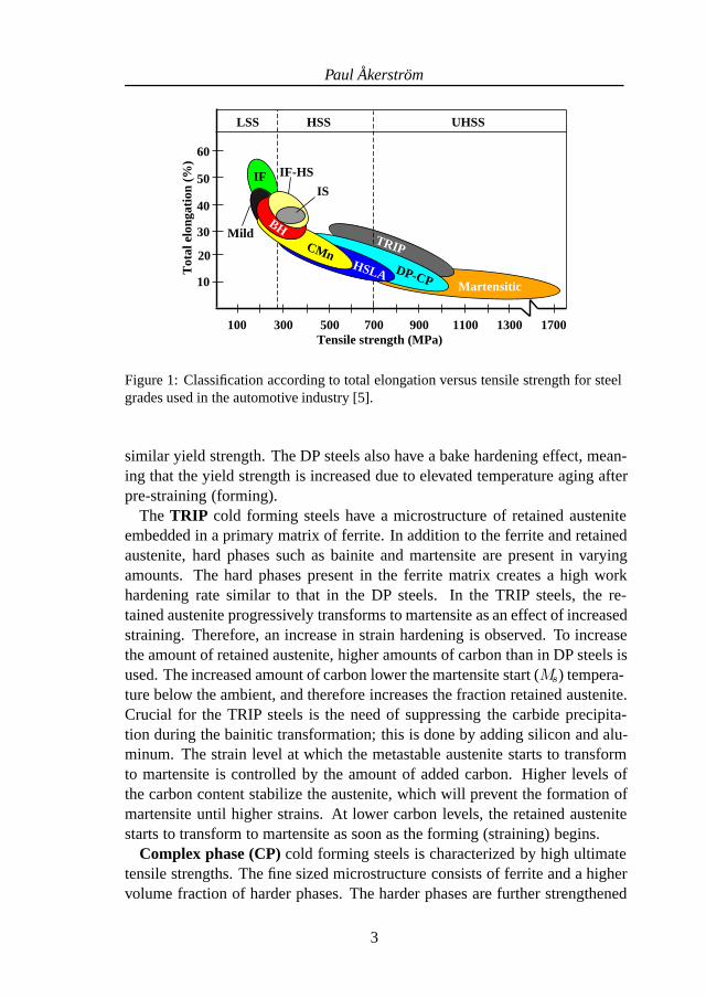
3. Mechanical properties - total elongation versus tensile strength
- See figure 1
A short description of the steels in the AHSS-group will be given, beginningwith the dual phase steel. DP steels are cold forming steels that consist of aferritic matrix with embedded islands of a hard martensitic second phase. In-creasing the volume fraction hard phase generally increases the strength. Thesoft ferrite is generally continuous, giving these steels good ductility. Dur-ing deformation, plastic strains will primarily concentrate in the soft ferritephase surrounding the hard martensitic islands, giving these steels a high work-hardening rate. The work-hardening rate in combination with good elongationgives DP steels higher ultimate tensile strengths than conventional steels of
1This category is often divided into several subclasses by steel manufacturers, e.g. mediumhigh strength steel, extra high strength steel.
2
Paul Akerstrom
Tensile strength (MPa)300100 500 700 1100900 1300 1700
LSS HSS UHSS
10
20
30
40
50
60
Tot
al e
long
atio
n (%
)
Martensitic
TRIP
DP-CPHSLA
CMn
IF
BH
IF-HS
IS
Mild
Figure 1: Classification according to total elongation versus tensile strength for steelgrades used in the automotive industry [5].
similar yield strength. The DP steels also have a bake hardening effect, mean-ing that the yield strength is increased due to elevated temperature aging afterpre-straining (forming).
The TRIP cold forming steels have a microstructure of retained austeniteembedded in a primary matrix of ferrite. In addition to the ferrite and retainedaustenite, hard phases such as bainite and martensite are present in varyingamounts. The hard phases present in the ferrite matrix creates a high workhardening rate similar to that in the DP steels. In the TRIP steels, the re-tained austenite progressively transforms to martensite as an effect of increasedstraining. Therefore, an increase in strain hardening is observed. To increasethe amount of retained austenite, higher amounts of carbon than in DP steels isused. The increased amount of carbon lower the martensite start (Ms) tempera-ture below the ambient, and therefore increases the fraction retained austenite.Crucial for the TRIP steels is the need of suppressing the carbide precipita-tion during the bainitic transformation; this is done by adding silicon and alu-minum. The strain level at which the metastable austenite starts to transformto martensite is controlled by the amount of added carbon. Higher levels ofthe carbon content stabilize the austenite, which will prevent the formation ofmartensite until higher strains. At lower carbon levels, the retained austenitestarts to transform to martensite as soon as the forming (straining) begins.
Complex phase (CP) cold forming steels is characterized by high ultimatetensile strengths. The fine sized microstructure consists of ferrite and a highervolume fraction of harder phases. The harder phases are further strengthened
3

Modelling and Simulation of Hot Stamping
by fine precipitates. To form the strengthening precipitates, small amounts ofthe alloying elements titanium, niobium and/or vanadium are added.
Martensitic cold forming steels are produced by quenching from the austeniticphase on the run-out table during hot-rolling or in the cooling section of thecontinuous annealing line. The obtained microstructure will consist of mainlymartensite. Martensitic steels provide the highest yield and tensile strengths, atthe expense of low ductility. To improve the ductility, post-quench temperingcan be employed.
1.4 Ultra high strength components in car body
The components in the car body that are commonly made of ultra high strengthsteels are shown in figure 2. The different components in accordance to figure2 are:
1. Door beam
2. Bumper beam
3. Cross and side members
4. A-/B- pillar reinforcement
5. Waist rail reinforcement
Figure 2: Components in car body using ultra high strength steel.
4
Paul Akerstrom
1.5 Hot stamping
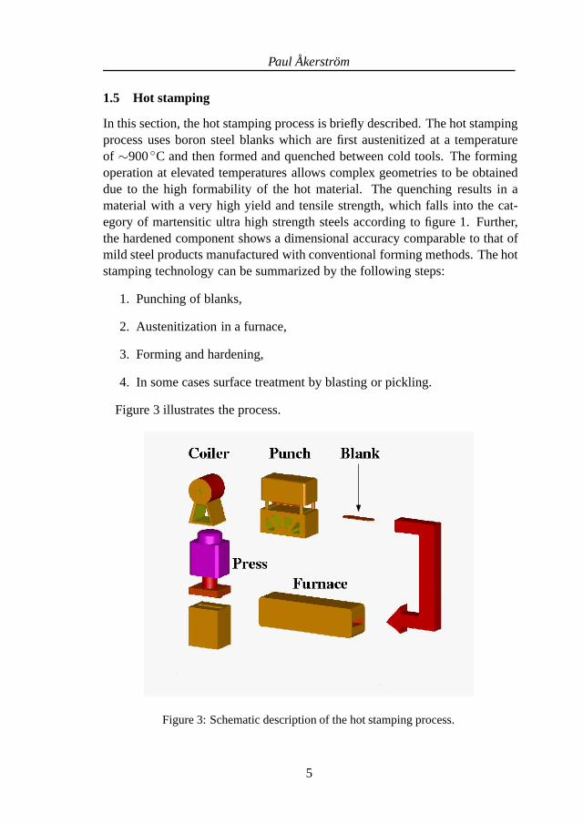
In this section, the hot stamping process is briefly described. The hot stampingprocess uses boron steel blanks which are first austenitized at a temperatureof ∼900 ◦C and then formed and quenched between cold tools. The formingoperation at elevated temperatures allows complex geometries to be obtaineddue to the high formability of the hot material. The quenching results in amaterial with a very high yield and tensile strength, which falls into the cat-egory of martensitic ultra high strength steels according to figure 1. Further,the hardened component shows a dimensional accuracy comparable to that ofmild steel products manufactured with conventional forming methods. The hotstamping technology can be summarized by the following steps:
1. Punching of blanks,
2. Austenitization in a furnace,
3. Forming and hardening,
4. In some cases surface treatment by blasting or pickling.
Figure 3 illustrates the process.
Figure 3: Schematic description of the hot stamping process.
5
Modelling and Simulation of Hot Stamping
1.6 Objective and Scope
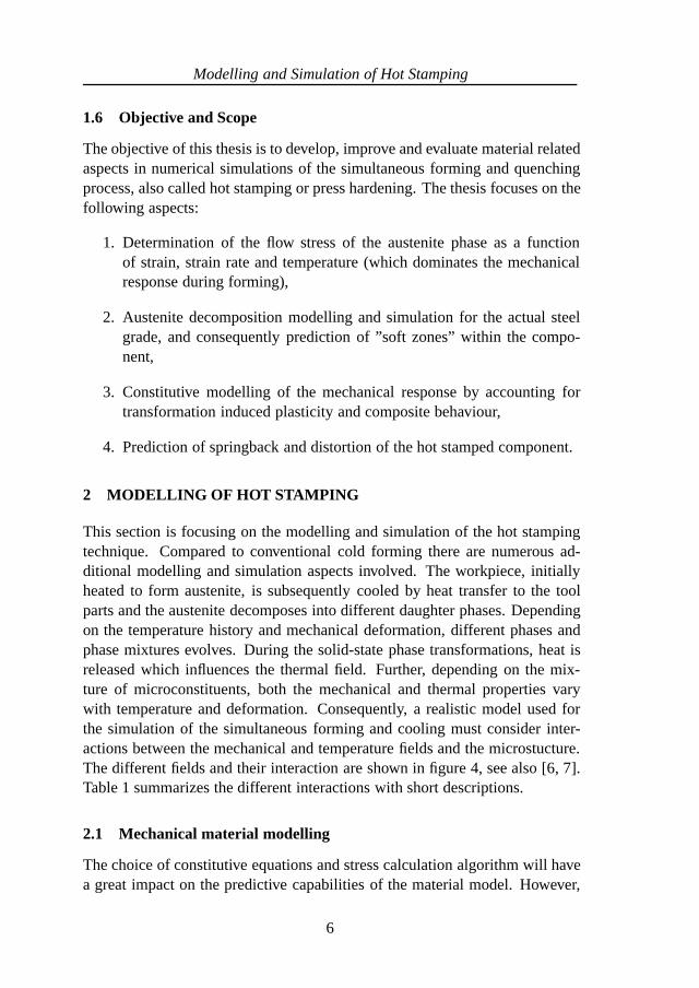
The objective of this thesis is to develop, improve and evaluate material relatedaspects in numerical simulations of the simultaneous forming and quenchingprocess, also called hot stamping or press hardening. The thesis focuses on thefollowing aspects:
1. Determination of the flow stress of the austenite phase as a functionof strain, strain rate and temperature (which dominates the mechanicalresponse during forming),
2. Austenite decomposition modelling and simulation for the actual steelgrade, and consequently prediction of ”soft zones” within the compo-nent,
3. Constitutive modelling of the mechanical response by accounting fortransformation induced plasticity and composite behaviour,
4. Prediction of springback and distortion of the hot stamped component.
2 MODELLING OF HOT STAMPING
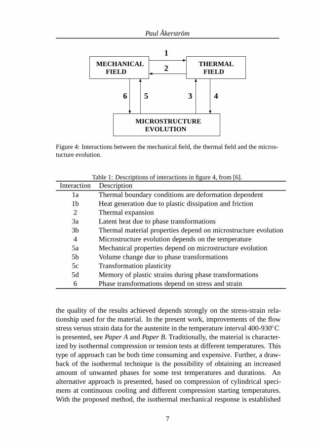
This section is focusing on the modelling and simulation of the hot stampingtechnique. Compared to conventional cold forming there are numerous ad-ditional modelling and simulation aspects involved. The workpiece, initiallyheated to form austenite, is subsequently cooled by heat transfer to the toolparts and the austenite decomposes into different daughter phases. Dependingon the temperature history and mechanical deformation, different phases andphase mixtures evolves. During the solid-state phase transformations, heat isreleased which influences the thermal field. Further, depending on the mix-ture of microconstituents, both the mechanical and thermal properties varywith temperature and deformation. Consequently, a realistic model used forthe simulation of the simultaneous forming and cooling must consider inter-actions between the mechanical and temperature fields and the microstucture.The different fields and their interaction are shown in figure 4, see also [6, 7].Table 1 summarizes the different interactions with short descriptions.
2.1 Mechanical material modelling
The choice of constitutive equations and stress calculation algorithm will havea great impact on the predictive capabilities of the material model. However,
6
Paul Akerstrom
MECHANICALFIELD
THERMALFIELD
MICROSTRUCTUREEVOLUTION
1
2
3 456
Figure 4: Interactions between the mechanical field, the thermal field and the micros-tucture evolution.
Table 1: Descriptions of interactions in figure 4, from [6].Interaction Description
1a Thermal boundary conditions are deformation dependent1b Heat generation due to plastic dissipation and friction2 Thermal expansion3a Latent heat due to phase transformations3b Thermal material properties depend on microstructure evolution4 Microstructure evolution depends on the temperature5a Mechanical properties depend on microstructure evolution5b Volume change due to phase transformations5c Transformation plasticity5d Memory of plastic strains during phase transformations6 Phase transformations depend on stress and strain
the quality of the results achieved depends strongly on the stress-strain rela-tionship used for the material. In the present work, improvements of the flowstress versus strain data for the austenite in the temperature interval 400-930◦Cis presented, see Paper A and Paper B. Traditionally, the material is character-ized by isothermal compression or tension tests at different temperatures. Thistype of approach can be both time consuming and expensive. Further, a draw-back of the isothermal technique is the possibility of obtaining an increasedamount of unwanted phases for some test temperatures and durations. Analternative approach is presented, based on compression of cylindrical speci-mens at continuous cooling and different compression starting temperatures.With the proposed method, the isothermal mechanical response is established
7
Modelling and Simulation of Hot Stamping
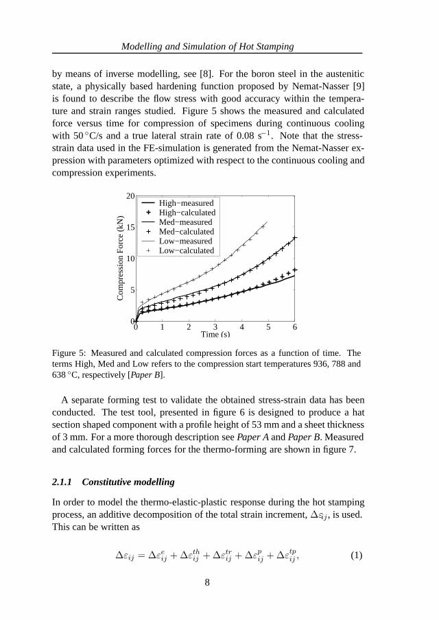
by means of inverse modelling, see [8]. For the boron steel in the austeniticstate, a physically based hardening function proposed by Nemat-Nasser [9]is found to describe the flow stress with good accuracy within the tempera-ture and strain ranges studied. Figure 5 shows the measured and calculatedforce versus time for compression of specimens during continuous coolingwith 50 ◦C/s and a true lateral strain rate of 0.08 s−1. Note that the stress-strain data used in the FE-simulation is generated from the Nemat-Nasser ex-pression with parameters optimized with respect to the continuous cooling andcompression experiments.
0 1 2 3 4 5 60
5
10
15
20
Time (s)
Com
pres
sion
For
ce (
kN)
High−measuredHigh−calculatedMed−measuredMed−calculatedLow−measuredLow−calculated
Figure 5: Measured and calculated compression forces as a function of time. Theterms High, Med and Low refers to the compression start temperatures 936, 788 and638 ◦C, respectively [Paper B].
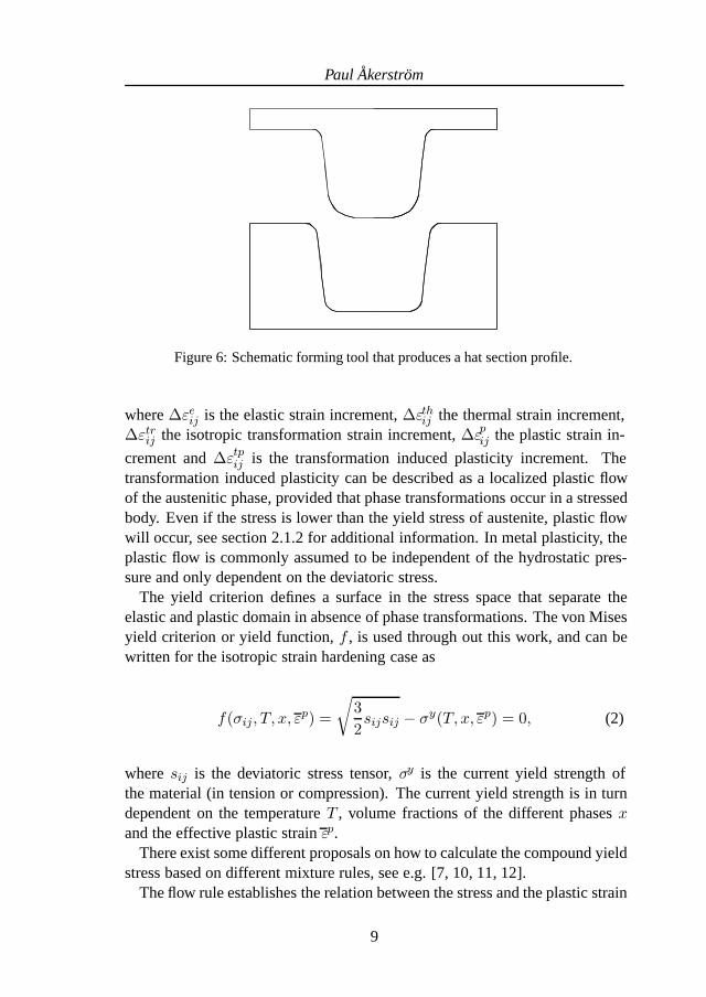
A separate forming test to validate the obtained stress-strain data has beenconducted. The test tool, presented in figure 6 is designed to produce a hatsection shaped component with a profile height of 53 mm and a sheet thicknessof 3 mm. For a more thorough description see Paper A and Paper B. Measuredand calculated forming forces for the thermo-forming are shown in figure 7.
2.1.1 Constitutive modelling
In order to model the thermo-elastic-plastic response during the hot stampingprocess, an additive decomposition of the total strain increment, Δεij , is used.This can be written as
Δεij = Δεeij + Δεth
ij + Δεtrij + Δεp
ij + Δεtpij , (1)
8
Paul Akerstrom
Figure 6: Schematic forming tool that produces a hat section profile.
where Δεeij is the elastic strain increment, Δεthij the thermal strain increment,
Δεtrij the isotropic transformation strain increment, Δεpij the plastic strain in-
crement and Δεtpij is the transformation induced plasticity increment. The
transformation induced plasticity can be described as a localized plastic flowof the austenitic phase, provided that phase transformations occur in a stressedbody. Even if the stress is lower than the yield stress of austenite, plastic flowwill occur, see section 2.1.2 for additional information. In metal plasticity, theplastic flow is commonly assumed to be independent of the hydrostatic pres-sure and only dependent on the deviatoric stress.
The yield criterion defines a surface in the stress space that separate theelastic and plastic domain in absence of phase transformations. The von Misesyield criterion or yield function, f , is used through out this work, and can bewritten for the isotropic strain hardening case as
f(σij, T, x, εp) =
√32sijsij − σy(T, x, εp) = 0, (2)
where sij is the deviatoric stress tensor, σy is the current yield strength ofthe material (in tension or compression). The current yield strength is in turndependent on the temperature T , volume fractions of the different phases xand the effective plastic strain εp.
There exist some different proposals on how to calculate the compound yieldstress based on different mixture rules, see e.g. [7, 10, 11, 12].
The flow rule establishes the relation between the stress and the plastic strain
9

Modelling and Simulation of Hot Stamping
0 1 2 3 4 50
5
10
15
20
25
Time (s)
Form
ing
Forc
e (k
N)
MeasuredCalculated − NNCalculated − TD
Figure 7: Measured and calculated forming forces as a function of time (NN - stressstrain data from optimized parameters in the Nemat-Nasser model; TD - stress straindata from iso-thermal tension tests).
increment Δεpij , see e.g. Fung and Tong [13], and can be written
Δεpij = Δλ
∂φ
∂σijfor Δλ ≥ 0, (3)
where Δλ is a factor of proportionality often referred to as the ”plastic multi-plier” and φ is a plastic potential function. In metal plasticity, the plastic flowdirection is normal to the yield surface as shown in figure 8. Therefore, thegeneral function φ in equation (3) is exchanged to the yield function given asequation (2).
σ1
σ3σ2
Δεijp
= Δλ ∂f∂σij
f < 0f = 0
Figure 8: Normality of the incremental plastic strains to the von Mises yield surfacein the deviatoric plane.
10
Paul Akerstrom
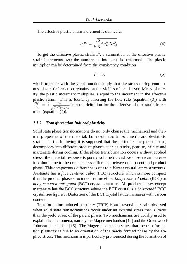
The effective plastic strain increment is defined as
Δεp =
√23Δεp
ijΔεpij . (4)
To get the effective plastic strain εp, a summation of the effective plasticstrain increments over the number of time steps is performed. The plasticmultiplier can be determined from the consistency condition
f = 0, (5)
which together with the yield function imply that the stress during continu-ous plastic deformation remains on the yield surface. In von Mises plastic-ity, the plastic increment multiplier is equal to the increment in the effectiveplastic strain. This is found by inserting the flow rule (equation (3)) with∂f
∂σij= 3
2sij√
(3/2)sijsijinto the definition for the effective plastic strain incre-
ment (equation (4)).
2.1.2 Transformation induced plasticity
Solid state phase transformations do not only change the mechanical and ther-mal properties of the material, but result also in volumetric and deviatoricstrains. In the following it is supposed that the austenite, the parent phase,decomposes into different product phases such as ferrite, pearlite, bainite andmartensite during cooling. If the phase transformation occurs without appliedstress, the material response is purely volumetric and we observe an increasein volume due to the compactness difference between the parent and productphase. This compactness difference is due to different crystal lattice structures.Austenite has a face centered cubic (FCC) structure which is more compactthan the product phase structures that are either body centered cubic (BCC) orbody centered tetragonal (BCT) crystal structure. All product phases exceptmartensite has the BCC structure where the BCT crystal is a ”distorted” BCCcrystal, see figure 9. Distortion of the BCT crystal lattice increases with carboncontent.
Transformation induced plasticity (TRIP) is an irreversible strain observedwhen solid state transformations occur under an external stress that is lowerthan the yield stress of the parent phase. Two mechanisms are usually used toexplain the phenomena, namely the Magee mechanism [14] and the Greenwood-Johnson mechanism [15]. The Magee mechanism states that the transforma-tion plasticity is due to an orientation of the newly formed phase by the ap-plied stress. This mechanism is particulary pronounced during the formation of
11

Modelling and Simulation of Hot Stamping
aa
c
Figure 9: BCT unit cell showing iron atoms as circles and sites that can be occupiedby carbon atoms as crosses, c > a.
martensite, which develop in form of plates and therefore generates high shear-ing in the austenite. When no external load is applied, the plates are generallyoriented randomly and therefore the macroscopic resultant of the microscopicstresses becomes negligible. An applied load generates internal stresses thatfavours certain directions for the formed martensite plates, which producesmicro stresses with a non-zero resultant and therefore generates transforma-tion plasticity. Transformation plasticity according to the Greenwood-Johnsonmechanism is based on the compactness difference between the austenite andthe product phase. Therefore, micro-stresses are introduced that generatesplastic strains in the soft austenite when an applied deviatoric stress is applied.If no external load is applied, no transformation plasticity is observed. This isdue to the nil volume average of the micro-plasticity. Therefore, macroscop-ically we can only expect a change in volume, see e.g. [16]. A commonlyused model in numerical simulations to account for the transformation plastic-ity due to the Greenwood-Johnson mechanism, is the model by Leblond andcoworkers [10, 17, 18, 19]. The transformation plasticity rate, εtpij , for thestrain hardening case is given as
εtpij = −3Δεth
1−2h(
σσy
)zln(z)
σy1(εp
1, T )sij, (6)
where Δεth1−2 is the difference in compactness between austenite and the prod-
12

Paul Akerstrom
uct phase, σy1 is the current yield stress of austenite, z is the volume fraction
product phase (0 ≤ z ≤ 1), sij is the deviatoric stress, h(
σσy
)is a correction
function accounting for the nonlinearity in the applied stress, defined as
h
(σ
σy
)=
{1 if σ
σy ≤ 12
1 + 3.5(
σσy − 1
2
)if σ
σy > 12 ,
(7)
where σ is the current effective stress and σy is the current global yield stressthat is a function of the current microconstituents and their deformation his-tory as well as the temperature. In paper D, a numerical implementation ofthe Leblond model is described. Figure 10 shows the measured and calcu-lated change in diameter for a loaded and unloaded cylindrical specimen whenaccounting for TRIP, from paper D.
100 200 300 400 500 600 700 800 900
−1.2
−1
−0.8
−0.6
−0.4
−0.2
0
Temperature (°C)
Cha
nge
in d
iam
eter
(%
)
CalculatedMeasured
σ33
= −165 MPa
σ33
= 0 MPa
σ33
= 112 MPa
Figure 10: Change in diameter as a function of temperature and axially applied forceon a cylindrical specimen.
Transformation plasticity models accounting for the orientation effect (Magee)during the martensitic transformation can be found in e.g. [20, 21].
2.2 Strain rate effects
Generally, ultra high strength and high strength steels exhibit a lower increasein flow stress when the strain rate is increased compared to low strength steels.The same is true for different micro-constituents, e.g. martensite shows a lowerrelative increase in flow stress than austenite or ferrite due to an increase instrain rate. To account for changes in the mechanical response due to increasedstrain rate, different approaches are commonly employed. Some of the mostcommonly used techniques are shortly summarized below;
13
Modelling and Simulation of Hot Stamping
• Stress-strain curves (points that defines a curve) for different strain ratesare given as input. If the actual strain rate fall between two given curves,linear interpolation is used to determine the actual flow stress and hard-ening.
• The use of expressions with parameters consistent with experimentalstress-strain data that account for changes in temperature and strain rate.An example is the flow stress expression given by Nemat-Nasser [9]. Itis shown in paper B that the Nemat-Nasser model capture the strain rateeffects in austenite with good accuracy.
• The use of visco-plastic constitutive relations, which use an empiricalfunction of stress and internal variables to determine the plastic rate pa-rameter instead of using the consistence condition as in rate-independentplasticity (section 2.1.1). The plastic rate parameter (plastic multiplier)in the visco-plastic formulation is typically given by an overstress func-tion. Different examples for overstress functions can be found in e.g.Belytschko et al. [3].
In FE-software using explicit time integration, very small time steps are used(often in the order of micro seconds) to ensure numerical stability. To reducethe total number of steps in a forming simulation, thus reduce the simulationtime, mass scaling or increased tool velocities are commonly applied. Whenusing an increased tool velocity, special treatment of the corresponding strainrate must be made. As done in Nielsen [22], a linear dependence is assumedbetween the increase in tool velocity and strain rate. Therefore, if the toolvelocity in the simulation is increased by a factor ϕ the corresponding strainrate is reduced with the factor 1/ϕ in the mechanical constitutive model. Thestrain rate effects for the different phases are currently not accounted for in theimplemented constitutive model.
2.3 Thermal modelling
2.3.1 Heat equation
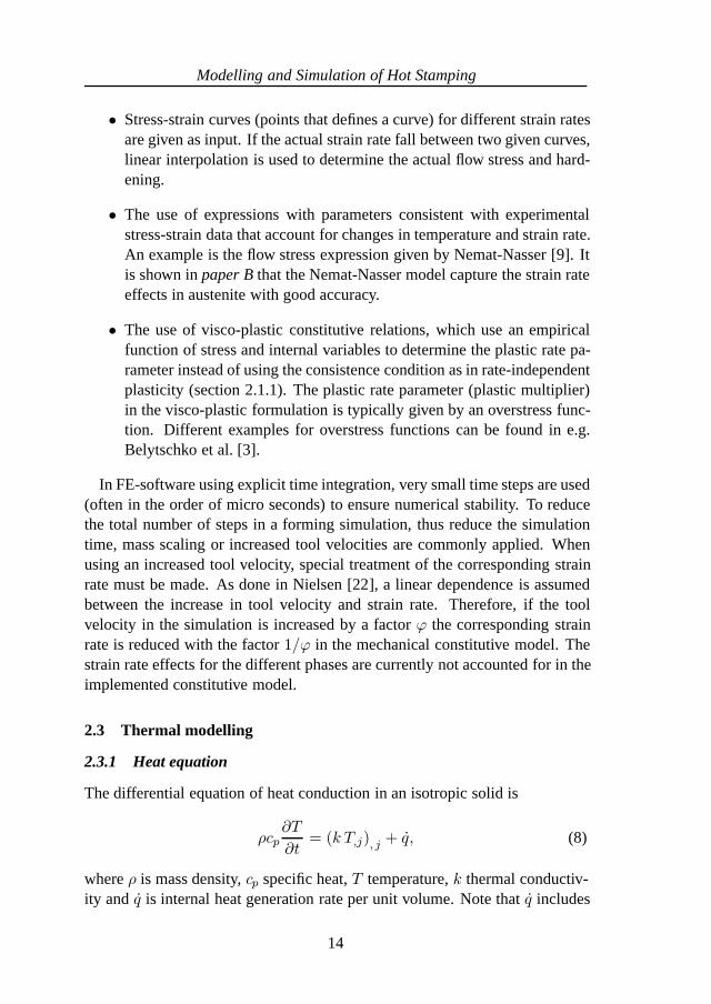
The differential equation of heat conduction in an isotropic solid is
ρcp∂T
∂t= (k T,j), j + q, (8)
where ρ is mass density, cp specific heat, T temperature, k thermal conductiv-ity and q is internal heat generation rate per unit volume. Note that q includes
14

Paul Akerstrom
Γp
Γt
Tt
n
P
Figure 11: Body subjected to heat transfer: prescribed temperature on Γ t and pre-scribed heat flow input on Γp.
external heat sources as well as transformation heat and heat generated byplastic deformation.
On the surfaces of the body (see figure 11), the following boundary condi-tions must be satisfied
T = Tt on Γt (9)
andk T,i ni = P on Γp, (10)
where Tt is a prescribed temperature on Γt, P is the prescribed heat flux onΓp and ni is the components of the outward unit normal vector n according tofigure 11. The heat flow input/output P may be prescribed at specific pointsand surfaces of the body and will be described in some more detail in section2.3.2. In addition to the boundary conditions, the temperature initial conditionsmust also be given in a transient analysis.
2.3.2 Boundary conditions - heat transfer
During the thermo-mechanical forming of the hot steel sheet in the tool, thesurface properties of the steel sheet varies with time due to oxidation and istherefore dependent on the type of pre-coating. Both the contact pressure andthe relative sliding in combination with the surface condition determine the
15
Modelling and Simulation of Hot Stamping
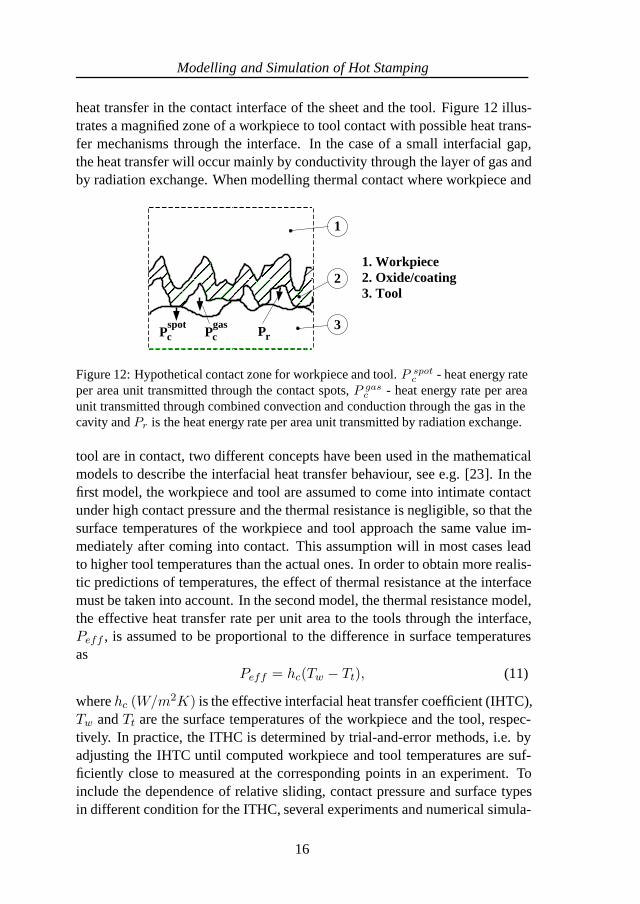
heat transfer in the contact interface of the sheet and the tool. Figure 12 illus-trates a magnified zone of a workpiece to tool contact with possible heat trans-fer mechanisms through the interface. In the case of a small interfacial gap,the heat transfer will occur mainly by conductivity through the layer of gas andby radiation exchange. When modelling thermal contact where workpiece and
1
2
3Pcspot
Pcgas
Pr
1. Workpiece2. Oxide/coating3. Tool
Figure 12: Hypothetical contact zone for workpiece and tool. P spotc - heat energy rate
per area unit transmitted through the contact spots, P gasc - heat energy rate per area
unit transmitted through combined convection and conduction through the gas in thecavity and Pr is the heat energy rate per area unit transmitted by radiation exchange.
tool are in contact, two different concepts have been used in the mathematicalmodels to describe the interfacial heat transfer behaviour, see e.g. [23]. In thefirst model, the workpiece and tool are assumed to come into intimate contactunder high contact pressure and the thermal resistance is negligible, so that thesurface temperatures of the workpiece and tool approach the same value im-mediately after coming into contact. This assumption will in most cases leadto higher tool temperatures than the actual ones. In order to obtain more realis-tic predictions of temperatures, the effect of thermal resistance at the interfacemust be taken into account. In the second model, the thermal resistance model,the effective heat transfer rate per unit area to the tools through the interface,Peff , is assumed to be proportional to the difference in surface temperaturesas
Peff = hc(Tw − Tt), (11)
where hc (W/m2K) is the effective interfacial heat transfer coefficient (IHTC),Tw and Tt are the surface temperatures of the workpiece and the tool, respec-tively. In practice, the ITHC is determined by trial-and-error methods, i.e. byadjusting the IHTC until computed workpiece and tool temperatures are suf-ficiently close to measured at the corresponding points in an experiment. Toinclude the dependence of relative sliding, contact pressure and surface typesin different condition for the ITHC, several experiments and numerical simula-
16

Paul Akerstrom
tions need to be performed. In many commercial FE-codes, it is not possible toinclude such dependencies, only constant values for the interfacial heat transfercoefficient is used.
For cases where the workpiece are far from the tool, the heat transfer fromthe sheet surface is due to convection to the surrounding air and by radiation.The emitted power per unit area, Pr due to radiation is calculated as
Pr = εσs
(T 4
w − T 4a
), (12)
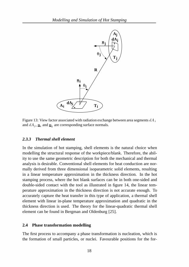
where ε is the emissivity, σs is the Stefan- Boltzmann constant, Tw and Ta arethe surface temperature of the workpiece and the ambient temperature, respec-tively. It should be noted that the emissivity is strongly dependent on the typeof surface on the workpiece, if the surface is oxidized, then the emissivity ishigher than for an oxide free. In equation (12) it is assumed the the workpieceis emitting without radiation exchange. If there are one or several surroundingsurfaces, one may account for the radiation exchange between the surfaces.This exchange depends strongly on the surface geometries and orientations, aswell as on their radiate properties and temperatures. To compute the radiationexchange between any two surfaces, the view factor, Fij is introduced. Fij isdefined as the fraction of the radiation leaving surface i which is interceptedby surface j. The expression for the view factor can be written2 [24]
Fij =1Ai
∫Ai
∫Aj
cosθicosθj
πR2dAjdAi, (13)
where the terms/variables used used in equation (13) are defined in figure 13.In the general case of radiation exchange, the emitted power from surface i
to the colder surface j can be written as
Pij = εeffσsFijAi
(T 4
i − T 4j
), (14)
where εeff is the effective emissivity.For the convective power per unit area, an expression of the same type as
in equation (11) is used. In this case, the heat transfer coefficient (HTC) isheavily reduced compared to the case of workpiece to tool contact and thetemperature Tt is exchanged to the ambient air temperature, Ta. Furthermore,the HTC coefficient is a function of the surface orientation, see e.g. [24].
2Indices appearing twice do not imply summation here.
17
Modelling and Simulation of Hot Stamping
Aj
Tj
jdAnj
TiAiidA
ni
θj
θi
R
Figure 13: View factor associated with radiation exchange between area segments dA i
and dAj , ni and nj are corresponding surface normals.
2.3.3 Thermal shell element
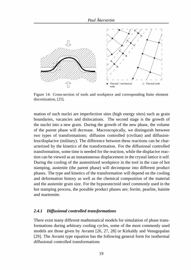
In the simulation of hot stamping, shell elements is the natural choice whenmodelling the structural response of the workpiece/blank. Therefore, the abil-ity to use the same geometric description for both the mechanical and thermalanalysis is desirable. Conventional shell elements for heat conduction are nor-mally derived from three dimensional isoparametric solid elements, resultingin a linear temperature approximation in the thickness direction. In the hotstamping process, where the hot blank surfaces can be in both one-sided anddouble-sided contact with the tool as illustrated in figure 14, the linear tem-perature approximation in the thickness direction is not accurate enough. Toaccurately capture the heat transfer in this type of application, a thermal shellelement with linear in-plane temperature approximation and quadratic in thethickness direction is used. The theory for the linear-quadratic thermal shellelement can be found in Bergman and Oldenburg [25].
2.4 Phase transformation modelling
The first process to accompany a phase transformation is nucleation, which isthe formation of small particles, or nuclei. Favourable positions for the for-
18
Paul Akerstrom
Thermal nodeThermal / mechanicalnode
Figure 14: Cross-section of tools and workpiece and corresponding finite elementdiscretization, [25].
mation of such nuclei are imperfection sites (high energy sites) such as grainboundaries, vacancies and dislocations. The second stage is the growth ofthe nuclei into a new grain. During the growth of the new phase, the volumeof the parent phase will decrease. Macroscopically, we distinguish betweentwo types of transformations; diffusion controlled (civilian) and diffusion-less/displacive (military). The difference between these reactions can be char-acterized by the kinetics of the transformation. For the diffusional controlledtransformation, some time is needed for the reaction, while the displacive reac-tion can be viewed as an instantaneous displacement in the crystal lattice it self.During the cooling of the austenitized workpiece in the tool in the case of hotstamping, austenite (the parent phase) will decompose into different productphases. The type and kinetics of the transformation will depend on the coolingand deformation history as well as the chemical composition of the materialand the austenite grain size. For the hypoeutectoid steel commonly used in thehot stamping process, the possible product phases are; ferrite, pearlite, bainiteand martensite.
2.4.1 Diffusional controlled transformations
There exist many different mathematical models for simulation of phase trans-formations during arbitrary cooling cycles, some of the most commonly usedmodels are those given by Avrami [26, 27, 28] or Kirkaldy and Venugopalan[29]. The Avrami type equation has the following general form for isothermaldiffusional controlled transformations
19

Modelling and Simulation of Hot Stamping
x = 1 − e−btn , (15)
where x is the fraction transformed, t is the time and b and n are constants.The values of b and n are chosen such that the calculated start and finish of thetransformation are in accordance with the experimentally determined data. Toextend the capability of the model to continuous cooling conditions, equation(15) is differentiated with respect to time to give
x = bntn−1e−btn . (16)
Equation (16) makes it possible to determine the amount of transformationproduct through time integration. If several product phases can form duringcooling, it would be necessary to modify the expression for the transformationrate to take into account the reduced amount of austenite available for trans-formation. For further details regarding numerical implementations of modelsbased on the Avrami type equations, see e.g. [7, 11, 30]
The model proposed by Kirkaldy and Venugopalan [29] can be written inthe general rate form for the diffusional controlled reactions as [31]
X = FGFCFT FX , (17)
where X is the rate of the normalized phase evolving, FG describes the effectof the austenite grain size, FC the effect of the chemical composition, FT is afunction of the temperature and FX gives the effect of the current normalizedfraction formed. Equation (17) describes a normalized reaction rate, i.e. thegrowth of a ghost fraction X which, initially at 0, reaches 1 at equilibrium.These ghost fractions are defined as the ratio of the momentary value to theequilibrium value. Li et al. [32] have modified the original model to improvethe predictions under continuous cooling conditions and also extended the ap-plicable chemical composition range.
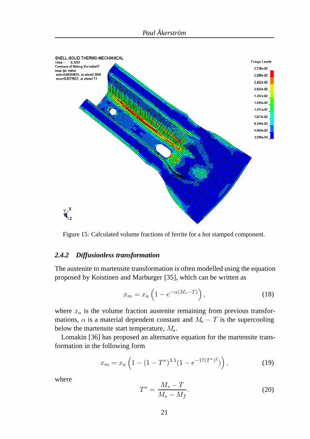
In the present work, the model proposed by Kirkaldy and Venugopalan [29]with and without modifications according to Li et al. [32] have been used.The overall computational algorithm for the phase transformations follow theone given in Watt et al. [33]. The model is implemented as a subroutine inthe FE-code LS-DYNA [34], see paper C and D. The calculated final volumefractions ferrite, for a hot stamped component is shown in figure 15 (from theFE-simulation in paper E).
20
Paul Akerstrom
Figure 15: Calculated volume fractions of ferrite for a hot stamped component.
2.4.2 Diffusionless transformation
The austenite to martensite transformation is often modelled using the equationproposed by Koistinen and Marburger [35], which can be written as
xm = xa
(1 − e−α(Ms−T )
), (18)
where xa is the volume fraction austenite remaining from previous transfor-mations, α is a material dependent constant and Ms − T is the supercoolingbelow the martensite start temperature, Ms.
Lomakin [36] has proposed an alternative equation for the martensite trans-formation in the following form
xm = xa
(1 − (1 − T ∗)3.5(1 − e−17(T ∗)2)
), (19)
where
T ∗ =Ms − T
Ms − Mf. (20)
21
Modelling and Simulation of Hot Stamping
In equation (20), Mf is the martensite finish temperature. In the present work,equation (18) is used to model the austenite to martensite reaction.
2.4.3 Effect of stress and strain on phase transformations
It has been shown in several works, see e.g. [37, 38, 39, 40], that the presenceof an applied or an internal stress affect both the martensite start temperature(Ms) and the fraction of martensite formed as function of the supercoolingbelow Ms. Inoue and Wang [39] have proposed an expression for the changein the martensite start temperature as
ΔMs = C1σm + C2
√J2, (21)
where σm is the mean stress, J2 is the second stress deviator and C1 and C2 areconstants. Generally, tensile and compressive normal stresses as well as shearstresses raises Ms. The hydrostatic component always decrease the martensitestart temperature. Liu et al. [40] has shown that the coefficient α in equation(18) is a function of the effective stress for lower stress levels, and a functionof both the effective stress and effective strain for higher levels of the appliedstress.
It has been shown that plastic straining of austenite accelerate the forma-tion of ferrite and increases the equilibrium ferrite volume fraction, see e.g.[41, 42, 43]. Explanations to these facts are given by Xiao et al. [43] and arehere briefly summarized. Firstly, the regions with high stored energy within theaustenite grains and the extended grain boundary area by plastic deformationwill increase the density of ferrite nucleation sites. Secondly, plastic defor-mation accelerate both the long-range diffusion of carbon atoms in austeniteas well as the short-range diffusion of iron atoms across the ferrite/austeniteinterface during the phase transformation. Based on the modification of theferrite kinetics given by Serajzadeh [42], an expression is added to the righthand side of equation (17) to account for the change in ferrite transformationkinetics by the plastic straining of austenite as
Fε =1
(1 − εpa)2
for εpa < 1, (22)
where εpa is the effective plastic strain in the austenite. This modification for
the ferrite kinetics is used in Paper D and E. Some discussions regarding theeffects of stress on the pearlite transformation can be found in e.g. Geijselaers[11]. For a detailed description regarding the effect of stress/strain on the bai-nite transformation, see Bhadeshia [44] and cites therein. In summary, the ef-fect of externally applied stress on the bainitic reaction is similar to those valid
22
Paul Akerstrom
for the martensite transformation. If the austenite is heavily deformed priorthe transformation to bainite, the transformation is retarded. The retardationof the transformation by plastic deformation is called mechanical stabilization,and is also observed for the austenite to martensite transformation. One expla-nation to the mechanical stabilization is that plastic straining of the austeniteincreases the amount of ferrite, which in turn gives an enrichment of carbonin austenite which shifts the bainite nose (in the cct-diagram) to longer timesas well as a decrease of the martensite start temperature. In the present work,the effects of stress and strain on the transformation to pearlite, bainite andmartensite are not accounted for. This omission is thought to have negligibleeffects.
2.4.4 Latent heat and change in thermal properties
During phase transformations, latent heat is released and therefore affects thethermal history. Furthermore, both the thermal conductivity and specific heatare changing as function of temperature and phase evolution. The generatedheat rate per unit volume, qtr , for each transformation product can be calcu-lated as [7]
qtr = ΔHx, (23)
where ΔH is the enthalpy of the transformation for the specific reaction and xis the transformation rate. To determine the material thermal conductivity andspecific heat, a linear rule of mixture is commonly used. This can be writtenas
y =N∑
k=1
xkyk(T ), (24)
where y is either the compound thermal conductivity or specific heat, xk is thevolume fraction of phase k, yk is the individual phase property that varies withtemperature and N is the number of phases present.
3 SUMMARY OF APPENDED PAPERS
3.1 Paper A
This work includes the determination of the high temperature response for theboron steel grade in its austenitic state. The developed method to determine theflow stress as a function of strain and temperature is based on a combinationof compression tests and inverse modelling. Different flow stress expressionshave been used in the inverse procedure to find out their capability to represent
23
Modelling and Simulation of Hot Stamping
the material behavior in the actual temperature and strain range. The obtainedmaterial data is used in a coupled thermo-mechanical FE-simulation that iscompared to corresponding experiment. The sheet is modelled with under-integrated Belytschko-Tsay shell elements [34] for the mechanical field andan element with constant through thickness temperature has been used for thethermal field. Simulated and tested forming forces are in fair agreement whichallow this procedure to be used in future applications.
3.1.1 Author’s contribution
The first author has made the numerical simulations, written most of the con-trol scripts and programs controlling the inverse modelling as well as writingthe paper. The compression tests has been conducted at Oulu University Fin-land. The validation experiment (hat section) was conducted together withLars Sandberg, SSAB HardTech AB. The corresponding FE-model/simulationwere conducted by the first author.
3.2 Paper B
In this paper, like the previous, the flow stress of austenite as a function oftemperature is estimated. The paper also covers the austenite response at thehigher strain rates that can appear during forming. Furthermore, the sensitivityand confidence intervals of the estimated parameters used to describe the flowstress are treated. In the validation simulation, a thermal shell element allowinga temperature variation through the thickness, described in [25], has been used.
3.2.1 Author’s contribution
The first author has made the numerical simulations, written most of the con-trol scripts and programs controlling the inverse modelling as well as writingmost of the paper. The confidence and sensitivity parts have been conductedin cooperation with Dr. Bengt Wikman (second author). For the experiments,see paper A.
3.3 Paper C
This paper treats the development of a numerical model that is capable of sim-ulate the austenite decomposition into daughter phases for the studied boronsteel. The model is based on the equations proposed by [29] and is includedas a subroutine in the commercial FE-code LS-DYNA [34]. Due to boronadditions in the steel, the start times and growth kinetics for the solid-state
24
Paul Akerstrom
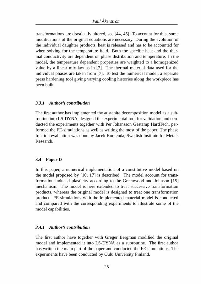
transformations are drastically altered, see [44, 45]. To account for this, somemodifications of the original equations are necessary. During the evolution ofthe individual daughter products, heat is released and has to be accounted forwhen solving for the temperature field. Both the specific heat and the ther-mal conductivity are dependent on phase distribution and temperature. In themodel, the temperature dependent properties are weighted to a homogenizedvalue by a linear mix law as in [7]. The thermal material data used for theindividual phases are taken from [7]. To test the numerical model, a separatepress hardening tool giving varying cooling histories along the workpiece hasbeen built.
3.3.1 Author’s contribution
The first author has implemented the austenite decomposition model as a sub-routine into LS-DYNA, designed the experimental tool for validation and con-ducted the experiments together with Per Johansson Gestamp HardTech, per-formed the FE-simulations as well as writing the most of the paper. The phasefraction evaluation was done by Jacek Komenda, Swedish Institute for MetalsResearch.
3.4 Paper D
In this paper, a numerical implementation of a constitutive model based onthe model proposed by [10, 17] is described. The model account for trans-formation induced plasticity according to the Greenwood and Johnson [15]mechanism. The model is here extended to treat successive transformationproducts, whereas the original model is designed to treat one transformationproduct. FE-simulations with the implemented material model is conductedand compared with the corresponding experiments to illustrate some of themodel capabilities.
3.4.1 Author’s contribution
The first author have together with Greger Bergman modified the originalmodel and implemented it into LS-DYNA as a subroutine. The first authorhas written the main part of the paper and conducted the FE-simulations. Theexperiments have been conducted by Oulu University Finland.
25

Modelling and Simulation of Hot Stamping
3.5 Paper E
In this paper a coupled thermo-mechanical FE-simulation of the production ofa hot stamped component using the models described in the previous papers isconducted. A corresponding experiment is performed and compared with thesimulation regarding:
• forming force,
• thickness distribution,
• hardness distribution,
• springback/shape accuracy.
In summary, simulation and experiment are in good agreement with accuracyenough for engineering applications.
3.5.1 Author’s contribution
The first author has designed the experiment tool used, created the correspond-ing FE-model and has written the main part of the paper. The experiments havebeen conducted together with Per Johansson at Gestamp HardTech Lulea.
4 DISCUSSION AND CONCLUSIONS
The objective of this thesis has been to implement variants of models availablein the open literature into a commercial FE-code for simulation of material re-sponse during hot stamping operations. Some effort has been directed to findmaterial data by a combination of experiments and inverse methods as well asexperiments only. The current work together with [6] is intended to improveand facilitate the design and development of ultra high strength componentswith the hot stamping technique. It has been shown that the used models givequite accurate predictions of the hot stamping process, both for the phase trans-formations and for the mechanical response. The main objective of the presentwork is the prediction of the shape accuracy of the final component after fin-ished forming. To be able to predict component distortion/shape accuracy, itis necessary to accurately predict the residual stress state. Therefore both thephase evolution model and mechanical model must give reliable results.
26
Paul Akerstrom
5 SUGGESTIONS FOR FUTURE WORK
There exist a number of aspects involved in the modelling and simulation ofthe hot stamping process that need to be further addressed. Some of these aregiven below without any order of priority.
1. Improved modelling of the frictional behavior by adding the dependenceof relative sliding, contact pressure, temperature and the type of surfacecoating or level of oxidation.
2. Improved modelling of the heat transfer between the workpiece andtools by adding the dependence of pressure, temperature, relative slidingand surface nature.
3. High temperature strain localization and failure.
4. Include orientation effects in the modelling of TRIP during the marten-sitic transformation.
5. Include effects of stress and strain on pearlitic and bainitic phase trans-formations.
6. Stress-strain behavior for individual phases as function of strain rate andtemperature.
7. Refined mix-laws to allow better estimation of the compound yield stressfor mixtures of several phases.
27
Modelling and Simulation of Hot Stamping
References
[1] R.D. Cook, D.S. Malkus, and M.E. Plesha. Concepts and applicationsof finite element analysis. John Wiley & Sons, New York, third edition,1989. ISBN 0-471-50319-3.
[2] K.-J. Bathe. Finite element procedures. Prentice Hall, Englewood Cliffs,N.J., 1996. ISBN 0-13-301458-4.
[3] T. Belytschko, W.K. Liu, and B. Moran. Nonlinear finite elements forcontinua and structures. John Wiley & Sons, New York, 2000. ISBN0-471-98774-3.
[4] R.W. Lewis, K. Morgan, H.R. Thomas, and K.N. Seetharamu. The finiteelement method in heat transfer analysis. John Wiley & Sons, New York,1996. ISBN 0-471-93424-0.
[5] International Iron and Steel Institute. Advanced high strength steel(AHSS) application guidelines. www.worldautosteel.org, 2005.
[6] G. Bergman. Modelling and simultaneous forming and quenching. PhDthesis, Lulea University of Technology, 1999.
[7] S. Sjostrom. The calculation of quench stresses in steel. PhD thesis,Linkoping University, 1982.
[8] M. Eriksson, B. Wikman, and G. Bergman. Estimations of material pa-rameters at elevated temperatures by inverse modelling of a gleeble ex-periment. In P. Stahle and K.G. Sundin, editors, IUTAM symposium onfield analyses for determination of material parameters - experimentaland numerical aspects, volume 109 of G.M.L. Gladwell, pages 151–165,Abisko Kiruna Sweden, 2000. Kluwer academic publishers.
[9] S. Nemat-Nasser. Experimental-based micro mechanical modelling ofmetal plasticity with homogenisation from micro- to macro-scale prop-erties. In O.T. Bruhns and E. Stein, editors, IUTAM symposium onmicro- and macro structural aspects of thermo plasticity, pages 101–113.Kluwer academic publishers, 1999.
[10] J.B. Leblond, G. Mottet, and J.C. Devaux. A theoretical and numericalapproach to the plastic behaviour of steels during phase transformations-2. study of classical plasticity for ideal-plastic phases. J. Mech. Phys.Solids, 34(4):411–432, 1986.
28
Paul Akerstrom
[11] H.J.M. Geijselaers. Numerical simulation of stresses due to solid statetransformations: The simulation of laser hardening. PhD thesis, Univer-sity of Twente, Twente Enschede The Netherlands, 2003.
[12] S. Petit-Grostabussiat, L. Taleb, and J-F. Jullien. Experimental resultson classical plasticity of steels subjected to structural transformations.International Journal of Plasticity, 20:1371–1386, 2004.
[13] Y.C. Fung and P. Tong. Classical and computational solid mechanics,volume 1. World Scientific Publishing Co. Pte. Ltd., 2001. ISBN 981-02-4124-0.
[14] C.L. Magee. Transformation kinetics, microplasticity and ageing ofmartensite in Fe-31-Ni. PhD thesis, Carnegie Institute of TechnologieUniversity, Pittsburgh, PA, 1966.
[15] G. W. Greenwood and R. H. Johnson. The deformation of metals undersmall stresses during phase transformations. volume 283, pages 403–422.Proc. Royal Society, 1965.
[16] L. Taleb, N. Cavallo, and F. Waeckel. Experimental analysis of transfor-mation plasticity. International Journal of Plasticity, 17:1–20, 2001.
[17] J.B. Leblond, G. Mottet, and J.C. Devaux. A theoretical and numericalapproach to the plastic behaviour of steels during phase transformations-1. derivation of general relations. J. Mech. Phys. Solids, 34(4):395–409,1986.
[18] J.B. Leblond, J. Devaux, and J.C. Devaux. Mathematical modelling oftransformation plasticity in steels 1: Case of ideal-plastic phases. Inter-national Journal of Plasticity, 5:551–572, 1989.
[19] J.B. Leblond. Mathematical modelling of transformation plasticity insteels 2: Coupling with strain hardening phenomena. International Jour-nal of Plasticity, 5:573–591, 1989.
[20] F.D. Fischer, Q.-P. Sun, and K. Tanaka. Transformation-induced plastic-ity (trip). Applied Mechanics Reviews, 49(6):317–364, 1996.
[21] F.D. Fischer, G. Reisner, E. Werner, K. Tanaka, G. Cailletaud, andT. Antretter. A new view on transformation induced plasticity. Inter-national Journal of Plasticity, 16:723–748, 2000.
29
Modelling and Simulation of Hot Stamping
[22] K. B. Nielsen. Sheet metal forming simulation using explicit finite ele-ment methods. PhD thesis, Aalborg University, Aalborg, Denmark, 1997.
[23] Y.H. Li and C.M. Sellars. Evaluation of interfacial heat transfer and fric-tion conditions and their effect on hot forming processes. In 37th me-chanical and steel processing conference, Hamilton, Ontario, Canada,October 1995. Iron and Steel Society Inc.
[24] F.P. Incropera and D.P. De Witt. Fundamentals of heat and mass transfer.John Wiley & Sons, New York, third edition, 1990. ISBN 0-471-51729-1.
[25] G. Bergman and M. Oldenburg. A finite element model for thermome-chanical analysis of sheet metal forming. Int. J. Numer. Meth. Eng., 59:1167–1186, 2004.
[26] M. Avrami. Kinetics of phase change 1 - general theory. J. Chem. Phys.,7:1103–1112, 1939.
[27] M. Avrami. Kinetics of phase change 2 - transformation-time relationsrandom distribution of nuclei. J. Chem. Phys., 8:212–224, 1940.
[28] M. Avrami. Kinetics of phase change 3 - granulation, phase change andmicrostructure. J. Chem. Phys., 9:177–184, 1941.
[29] J.S. Kirkaldy and D. Venugopalan. Prediction of microstructure and hard-enability in low alloy steels. In A.R. Marder and J.I. Goldstein, editors,Int. conference on phase transformations in ferrous alloys, pages 125–148, Philadelphia, Oct. 1983.
[30] B. Hildenwall. Prediction of the residual stresses created during quench-ing. PhD thesis, Linkoping University, 1979.
[31] A.S. Oddy, J.M.J. McDill, and L. Karlsson. Microstructural predictionsincluding arbitrary thermal histories, reaustenitization and carbon segre-gation effects. Canadian Metallurgical Quartely, 35(3):275–283, 1996.
[32] M.V. Li, D.V. Niebuhr, L.L. Meekisho, and D.G. Atteridge. A computa-tional model for the prediction of steel hardenability. Metallurgical andMaterials Transactions, 29B(3):661–672, June 1998.
[33] D. Watt, L. Coon, M. Bibby, J. Goldak, and C. Henwood. An algorithmfor modelling microstructural development in weld heat-affected zones(part a) reaction kinetics. Acta Metallurgica, 36(11):3029–3035, 1988.
30

Paul Akerstrom
[34] J.O. Hallquist. LS-DYNA theoretical manual. LSTC, Nov. 2005.
[35] D.P. Koistinen and R.E. Marburger. A general equation prescribing theextent of the austenite-martensite transformations in pure iron-carbon al-loys and plain carbon steels. Acta Metall., 36:59–60, 1959.
[36] V.A. Lomakin. Transformation of austenite under nonisothermal cooling.Mech. and Machine, 2:20–25, 1958.
[37] J.R. Patel and M. Cohen. Criterion for the action of applied stress in themartensitic transformation. Acta Metall., 1:581–538, 1953.
[38] S. Denis, A. Simon, and G. Beck. Estimation of the effect ofstress/phase transformation interaction when calculating internal stressduring martensitic quenching of steel. Transactions ISIJ, 22:504–513,1982.
[39] T. Inoue and Z. Wang. Coupling between stress, temperature and metallicstructures during processes involving phase transformations. MaterialScience and Technology, 1(10):845–850, 1985.
[40] C. Liu, K.-F. Yau, Z. Liu, and G. Gau. Study of the effects of stress andstrain on martensite transformation: kinetics and transformation plastic-ity. Journal of Computer-Aided Materials Design, 7:63–69, 2000.
[41] M.C. Somani, L.P. Karjalainen, M. Eriksson, and M. Oldenburg. Di-mensional changes and microstructural evolution in a b-bearing steel inthe simulated forming and quenching process. ISIJ International, 41(4):361–367, 2001.
[42] S. Serajzadeh. Modelling of temperature history and phase transforma-tions during cooling of steel. Journal of Materials Science and Engineer-ing, 146:311–317, 2004.
[43] N. Xiao, M. Tong, Y. Lan, D. Li, and Y. Li. Coupled simulation of the in-fluence of austenite deformation on the subsequent isothermal austenite-ferrite transformation. Acta Materialia, 54:1265–1278, March 2006.
[44] B.K.D.H. Bhadeshia. Bainite in steels, volume 2. Institute of Materials,2001. ISBN 1-86125-112-2.
[45] J.E. Morral and T.B. Cameron. Boron hardenability mechanisms. InS.K. Banerji et al., editor, Int. symposium on boron steels: Boron in steel,pages 19–32, Milwaukee Wisconsin USA, 1979.
31


Paper A

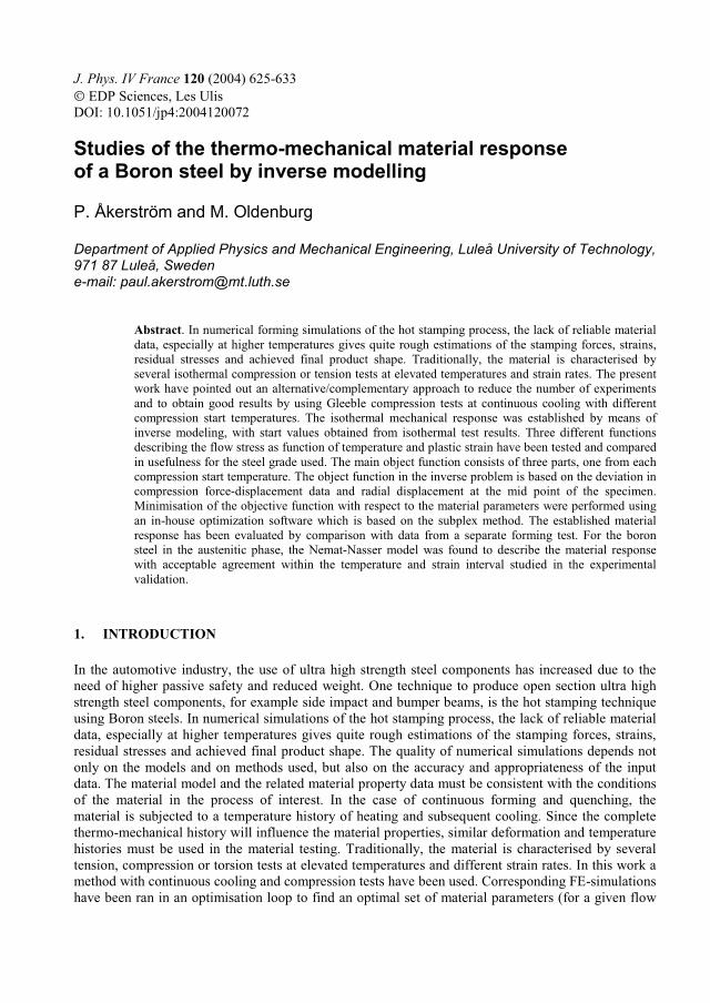
J. Phys. IV France 120 (2004) 625-633 � EDP Sciences, Les Ulis DOI: 10.1051/jp4:2004120072 Studies of the thermo-mechanical material response of a Boron steel by inverse modelling P. Åkerström and M. Oldenburg Department of Applied Physics and Mechanical Engineering, Luleå University of Technology, 971 87 Luleå, Sweden e-mail: [email protected]
Abstract. In numerical forming simulations of the hot stamping process, the lack of reliable material data, especially at higher temperatures gives quite rough estimations of the stamping forces, strains, residual stresses and achieved final product shape. Traditionally, the material is characterised by several isothermal compression or tension tests at elevated temperatures and strain rates. The present work have pointed out an alternative/complementary approach to reduce the number of experiments and to obtain good results by using Gleeble compression tests at continuous cooling with different compression start temperatures. The isothermal mechanical response was established by means of inverse modeling, with start values obtained from isothermal test results. Three different functions describing the flow stress as function of temperature and plastic strain have been tested and compared in usefulness for the steel grade used. The main object function consists of three parts, one from each compression start temperature. The object function in the inverse problem is based on the deviation in compression force-displacement data and radial displacement at the mid point of the specimen. Minimisation of the objective function with respect to the material parameters were performed using an in-house optimization software which is based on the subplex method. The established material response has been evaluated by comparison with data from a separate forming test. For the boron steel in the austenitic phase, the Nemat-Nasser model was found to describe the material response with acceptable agreement within the temperature and strain interval studied in the experimental validation.
1. INTRODUCTION In the automotive industry, the use of ultra high strength steel components has increased due to the need of higher passive safety and reduced weight. One technique to produce open section ultra high strength steel components, for example side impact and bumper beams, is the hot stamping technique using Boron steels. In numerical simulations of the hot stamping process, the lack of reliable material data, especially at higher temperatures gives quite rough estimations of the stamping forces, strains, residual stresses and achieved final product shape. The quality of numerical simulations depends not only on the models and on methods used, but also on the accuracy and appropriateness of the input data. The material model and the related material property data must be consistent with the conditions of the material in the process of interest. In the case of continuous forming and quenching, the material is subjected to a temperature history of heating and subsequent cooling. Since the complete thermo-mechanical history will influence the material properties, similar deformation and temperature histories must be used in the material testing. Traditionally, the material is characterised by several tension, compression or torsion tests at elevated temperatures and different strain rates. In this work a method with continuous cooling and compression tests have been used. Corresponding FE-simulations have been ran in an optimisation loop to find an optimal set of material parameters (for a given flow
JOURNAL DE PHYSIQUE IV
626
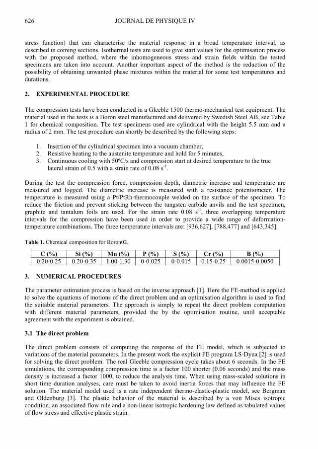
stress function) that can characterise the material response in a broad temperature interval, as described in coming sections. Isothermal tests are used to give start values for the optimisation process with the proposed method, where the inhomogeneous stress and strain fields within the tested specimens are taken into account. Another important aspect of the method is the reduction of the possibility of obtaining unwanted phase mixtures within the material for some test temperatures and durations. 2. EXPERIMENTAL PROCEDURE The compression tests have been conducted in a Gleeble 1500 thermo-mechanical test equipment. The material used in the tests is a Boron steel manufactured and delivered by Swedish Steel AB, see Table 1 for chemical composition. The test specimens used are cylindrical with the height 5.5 mm and a radius of 2 mm. The test procedure can shortly be described by the following steps:
1. Insertion of the cylindrical specimen into a vacuum chamber, 2. Resistive heating to the austenite temperature and hold for 5 minutes, 3. Continuous cooling with 50ºC/s and compression start at desired temperature to the true
lateral strain of 0.5 with a strain rate of 0.08 s-1. During the test the compression force, compression depth, diametric increase and temperature are measured and logged. The diametric increase is measured with a resistance potentiometer. The temperature is measured using a Pt/PtRh-thermocouple welded on the surface of the specimen. To reduce the friction and prevent sticking between the tungsten carbide anvils and the test specimen, graphite and tantalum foils are used. For the strain rate 0.08 s-1, three overlapping temperature intervals for the compression have been used in order to provide a wide range of deformation-temperature combinations. The three temperature intervals are: [936,627], [788,477] and [643,345]. Table 1. Chemical composition for Boron02.
C (%) Si (%) Mn (%) P (%) S (%) Cr (%) B (%) 0.20-0.25 0.20-0.35 1.00-1.30 0-0.025 0-0.015 0.15-0.25 0.0015-0.0050
3. NUMERICAL PROCEDURES The parameter estimation process is based on the inverse approach [1]. Here the FE-method is applied to solve the equations of motions of the direct problem and an optimisation algorithm is used to find the suitable material parameters. The approach is simply to repeat the direct problem computation with different material parameters, provided the by the optimisation routine, until acceptable agreement with the experiment is obtained. 3.1 The direct problem The direct problem consists of computing the response of the FE model, which is subjected to variations of the material parameters. In the present work the explicit FE program LS-Dyna [2] is used for solving the direct problem. The real Gleeble compression cycle takes about 6 seconds. In the FE simulations, the corresponding compression time is a factor 100 shorter (0.06 seconds) and the mass density is increased a factor 1000, to reduce the analysis time. When using mass-scaled solutions in short time duration analyses, care must be taken to avoid inertia forces that may influence the FE solution. The material model used is a rate independent thermo-elastic-plastic model, see Bergman and Oldenburg [3]. The plastic behavior of the material is described by a von Mises isotropic condition, an associated flow rule and a non-linear isotropic hardening law defined as tabulated values of flow stress and effective plastic strain.
ICTPMCS
627
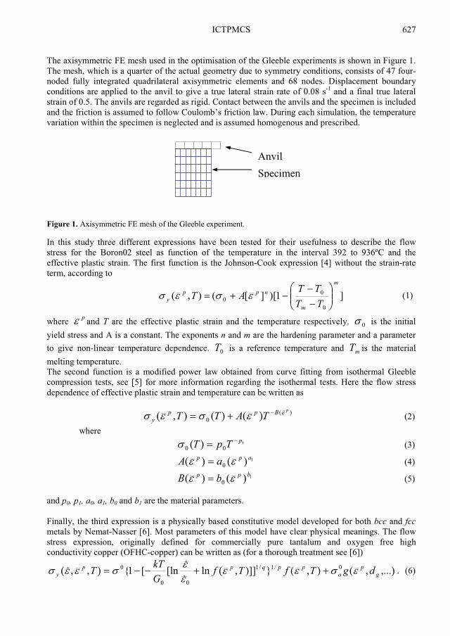
The axisymmetric FE mesh used in the optimisation of the Gleeble experiments is shown in Figure 1. The mesh, which is a quarter of the actual geometry due to symmetry conditions, consists of 47 four-noded fully integrated quadrilateral axisymmetric elements and 68 nodes. Displacement boundary conditions are applied to the anvil to give a true lateral strain rate of 0.08 s-1 and a final true lateral strain of 0.5. The anvils are regarded as rigid. Contact between the anvils and the specimen is included and the friction is assumed to follow Coulomb’s friction law. During each simulation, the temperature variation within the specimen is neglected and is assumed homogenous and prescribed.
Figure 1. Axisymmetric FE mesh of the Gleeble experiment. In this study three different expressions have been tested for their usefulness to describe the flow stress for the Boron02 steel as function of the temperature in the interval 392 to 936ºC and the effective plastic strain. The first function is the Johnson-Cook expression [4] without the strain-rate term, according to
]1)[][(),(0
00
m
m
nppy TT
TTAT
��
�
�
��
�
�
�
�
� ���� (1)
where p� and T are the effective plastic strain and the temperature respectively. 0� is the initial
yield stress and A is a constant. The exponents n and m are the hardening parameter and a parameter to give non-linear temperature dependence. 0T is a reference temperature and mT is the material melting temperature. The second function is a modified power law obtained from curve fitting from isothermal Gleeble compression tests, see [5] for more information regarding the isothermal tests. Here the flow stress dependence of effective plastic strain and temperature can be written as
)(0 )()(),(
pBppy TATT �
����
�
�� (2) where
100 )( pTpT �
�� (3) 1)()( 0
app aA �� � (4) 1)()( 0
bpp bB �� � (5) and p0, p1, a0, a1, b0 and b1 are the material parameters. Finally, the third expression is a physically based constitutive model developed for both bcc and fcc metals by Nemat-Nasser [6]. Most parameters of this model have clear physical meanings. The flow stress expression, originally defined for commercially pure tantalum and oxygen free high conductivity copper (OFHC-copper) can be written as (for a thorough treatment see [6])
,...),(),(})]],(ln[ln[1{),,( 0/1/1
00
0g
pa
ppqppy dgTfTf
GkTT ����
�
�
���� �����
�
�� . (6)
AnvilSpecimen

JOURNAL DE PHYSIQUE IV
628
In (6), �� is the effective strain rate, p� is the effective plastic strain, T is the temperature, 0
� is an effective stress to be determined empirically, k is Stefan Boltzman constant, G0 is the magnitude of the energy barrier that the dislocations must overcome. 0�� is a reference strain rate related to the density
and the average velocity of the mobile dislocations and the barrier spacing. The function ),( Tf p� is
defined in sequel for fcc metals, and ,...),(0g
pa dg �� is the athermal part of the flow stress. The
parameters p and q define the shape of the energy barrier (not the same p as the superscript in p�
where it means “plastic”). As for the OFHC copper, the following representation is assumed to work sufficient good for the austenitic state of the Boron steel
pp TaTf �� )(1),( �� (7) })/(1{)( 2
0 mTTaTa �� (8) where Tm is the melting temperature, and a0 depends on the initial average dislocation spacing. The last term in (6), ,...),( g
p dg � is approximated by 1)(,...),( np
gp dg �� � . (9)
In this flow stress function there are 8 material parameters to be determined. 3.2 The inverse problem The solution of the direct problem gives the necessary input information to the inverse problem. In the Gleeble application, the FE simulation provides output data in the form of axial reaction force and radial increase at mid-height (surface) of the specimen as function of the material parameters and the friction coefficient. In this work, three different FE analyses and corresponding test results have been used for the definition of the objective function. The FE analyses have been ran in parallel on different machines in a Linux cluster to reduce the analysis time. The objective of the inverse problem is to find the material parameters, which gives the best match between the FE solutions and the experimental reference data. This procedure is however not straightforward, because the data cannot be matched exactly. An optimisation approach is utilised for estimating the material parameters, which minimise the following objective function
)()(3
1ik
kitot DD ��
�
�� , i = 1,2,...,M (10)
where 2
exp
exp2
exp
exp
1
)()(21)(
�
�
�
�
�
�
�
� �
�
�
�
�
�
�
�
� �
�
� j
ifem
jj
j
ifem
jjN
jik r
Drrf
DffD
k
� (11)
Here expexp ,, jfem
jj rff and femjr are the experimental and calculated forces and radial increases for
point j on respective curve. Di denotes the M different material parameters and the terms exp/1 jf and exp/1 jr are normalisation or weight factors that are applied to avoid adding terms of diverse orders of
magnitude. The minimum of �k(Di) in Equation (11) gives a closest match in a least-square sense between the Nk sample points of each FE solution and corresponding experimental data (index k is used to represent the different temperature intervals). In searching for the minimum value of the objective function tot� , the subplex algorithm, Rowan [7], has been used. The inverse problem is solved by a set of customised subprograms; analyser programs, interface programs and a connecting network. Figure 2 shows a schematic structure of the optimisation process.

ICTPMCS
629
Integrate the equations of motionfor models of the experiment by usingLs-Dyna for each temperature intervaland a new set of design variables.
Minimise the total objectivefunction using the subplex method.
START
FEM Optimisation
STOP Figure 2. Basic flowchart of the inverse problem. 4. RESULTS The results in this section will be divided into three main sections, one for each tested flow stress expression. Separate optimisations have been conducted to get material parameters that best fit stress strain curves from isothermal compression tests, conducted in [5], which should provide relatively good start values. The friction between the tungsten carbide anvils, tantalum foil, graphite foil and the Boron specimen in the vacuum chamber at specific temperatures is known to be of a complex nature. Frictional data for this type of multi solid body contact in a vacuum chamber is not readily available. The static and dynamical frictional coefficients are non-linear functions of relative sliding velocity, contact pressure, temperature, atmosphere and the nature of the surfaces. Normally at room temperature and normal atmosphere, the friction coefficient in steel to graphite contact is about 0.1, from Bowden and Tabur [8]. When studying the specimens after the test, it can be seen that the bulging effect is quite moderate, indicating that the friction coefficient between the specimen and the foils is relatively low. For the two first flow stress expressions, a constant friction coefficient of 0.08 is assumed (both static and dynamic). For the third expression, Nemat-Nasser, different constant friction coefficients have been tested, and in one optimisation run the friction coefficient has been included as a design variable. 4.1 Johnson-Cook In the pre-optimisation for finding start values, the Johnson-Cook flow stress expression (1), showed an insufficient ability to represent the stress-strain curves from the isothermal compression tests. Here the isothermal curves are assumed not to differ much from the “correct” stress-strain curves in the temperature interval, 400-900�C, and to give sufficient good start parameters for the inverse Gleeble run. The inverse analysis converged after 267 iterations, ending with a objective function value of 15.52. Initial and optimised material parameters from the Gleeble inverse analysis are shown in Table 2, with specified parameter limits used in the optimisation. Table 2. Material parameters with limits used in the inverse problem for the J-Cook model.
Parameter Initial value Estimated value Parameter limits �0 1.39204*102 1.04447 0.0 < �0 < 1.0*103 A 2.26606*103 4.63254*103 0.0 < A < 5.0*104 n 2.71344*10-1 2.53198*10-1 0.0 < n < 5.0 m 2.45381*10-1 1.24533*10-1 0.0 < m < 5.0
4.2 Modified power law The results from this flow stress expression shows better agreement with the experimental results. For temperatures lower than 500�C, the model seems to overestimate the flow stress, due to restrictions in
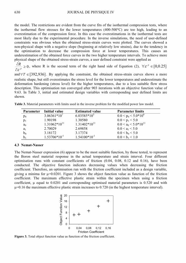
JOURNAL DE PHYSIQUE IV
630
the model. The restrictions are evident from the curve fits of the isothermal compression tests, where the isothermal flow stresses for the lower temperatures (400-500�C) are too high, leading to an overestimation of the compression force. In this case the overestimations in the isothermal tests are most likely due to the experimental procedure. In the inverse simulations, the need of user-defined constraints was obvious when the obtained stress-strain curves were plotted. The curves showed a non-physical shape with a negative slope (beginning at relatively low strains), due to the tendency in the optimisation to decrease the compression force at lower temperatures. This causes an underestimation of the obtained force curves in the two higher temperature intervals. To achieve more physical shape of the obtained stress-strain curves, a user defined constraint were applied as
0�
�
�
p
R�
, where R is the second term of the right hand side of Equation (2), ]25.0,0[��
p�
and T� ]936,392[� . By applying the constraint, the obtained stress-strain curves shows a more realistic shape, but still overestimates the stress level for the lower temperatures and underestimate the deformation hardening (stress level) for the higher temperatures, due to a less suitable flow stress description. This optimisation run converged after 903 iterations with an objective function value of 9.63. In Table 3, initial and estimated design variables with corresponding user defined limits are shown. Table 3. Material parameters with limits used in the inverse problem for the modified power law model.
Parameter Initial value Estimated value Parameter limits p0 3.06361*107 6.03585*105 0.0 < p0 < 5.0*108 p1 1.90198 1.30580 0.0 < p1 < 5.0 a0 1.31062*1011 1.31402*1011 0.0 < a0 < 5.0*1011 a1 2.70029 2.69858 0.0 < a1 < 5.0 b0 3.18172 3.17374 0.0 < b0 < 5.0 b1 1.53706*10-1 1.54100*10-1 0.0 < b1 < 1.0
4.3 Nemat-Nasser The Nemat-Nasser expression (6) appear to be the most suitable function, by those tested, to represent the Boron steel material response in the actual temperature and strain interval. Four different optimisation runs with constant coefficients of friction (0.04, 0.08, 0.12 and 0.16), have been conducted. The objective function indicates decreasing values when decreasing the friction coefficient. Therefore, an optimisation run with the friction coefficient included as a design variable, giving a minima for �=0.0201. Figure 3 shows the object function value as function of the friction coefficient. The maximum effective plastic strain within the specimen when using a friction coefficient, � equal to 0.0201 and corresponding optimised material parameters is 0.520 and with �=0.16 the maximum effective plastic strain increases to 0.720 (in the highest temperature interval).
0
4
8
12
16
20
0 0,04 0,08 0,12 0,16
Friction Coefficient
Ob
ject
Fu
nctio
n V
alu
e
Figure 3. Total object function value as function of the friction coefficient.
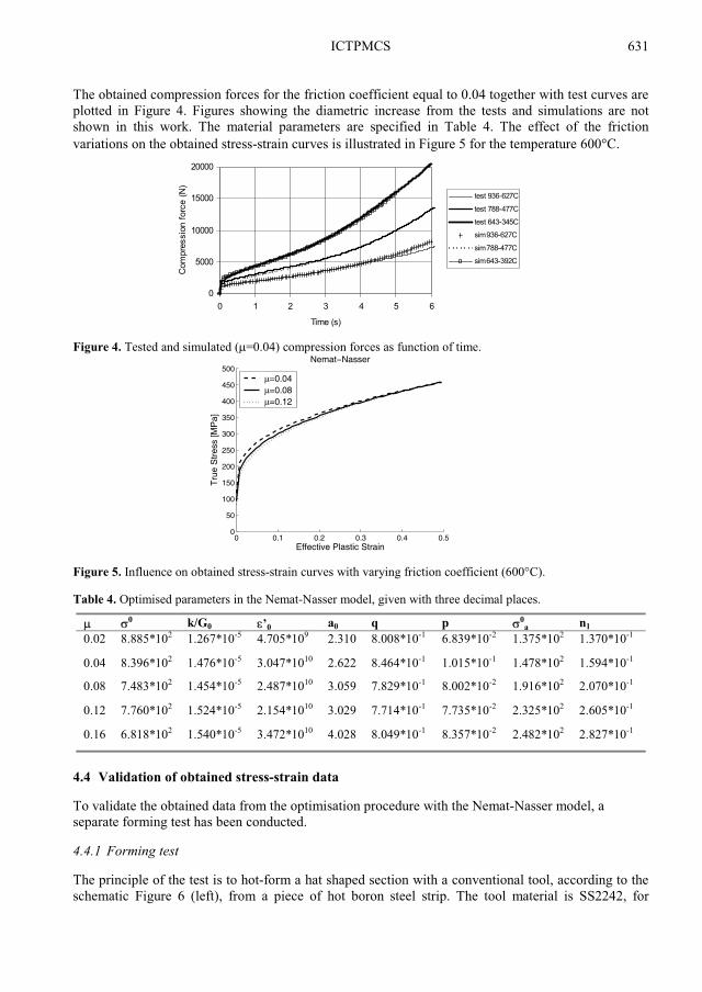
ICTPMCS
631
The obtained compression forces for the friction coefficient equal to 0.04 together with test curves are plotted in Figure 4. Figures showing the diametric increase from the tests and simulations are not shown in this work. The material parameters are specified in Table 4. The effect of the friction variations on the obtained stress-strain curves is illustrated in Figure 5 for the temperature 600�C. Figure 4. Tested and simulated (�=0.04) compression forces as function of time. Figure 5. Influence on obtained stress-strain curves with varying friction coefficient (600�C). Table 4. Optimised parameters in the Nemat-Nasser model, given with three decimal places.
� �
0 k/G0 �’0 a0 q p �
0a n1
0.02 8.885*102 1.267*10-5 4.705*109 2.310 8.008*10-1 6.839*10-2 1.375*102 1.370*10-1
0.04 8.396*102 1.476*10-5 3.047*1010 2.622 8.464*10-1 1.015*10-1 1.478*102 1.594*10-1
0.08 7.483*102 1.454*10-5 2.487*1010 3.059 7.829*10-1 8.002*10-2 1.916*102 2.070*10-1
0.12 7.760*102 1.524*10-5 2.154*1010 3.029 7.714*10-1 7.735*10-2 2.325*102 2.605*10-1
0.16 6.818*102 1.540*10-5 3.472*1010 4.028 8.049*10-1 8.357*10-2 2.482*102 2.827*10-1
4.4 Validation of obtained stress-strain data To validate the obtained data from the optimisation procedure with the Nemat-Nasser model, a separate forming test has been conducted. 4.4.1 Forming test The principle of the test is to hot-form a hat shaped section with a conventional tool, according to the schematic Figure 6 (left), from a piece of hot boron steel strip. The tool material is SS2242, for
0
5000
10000
15000
20000
0 1 2 3 4 5 6
Time (s)
Com
pre
ssio
n f
orc
e (
N)
test 936-627C
test 788-477C
test 643-345C
sim 936-627C
sim 788-477C
sim 643-392C
0 0.1 0.2 0.3 0.4 0.50
50
100
150
200
250
300
350
400
450
500Nemat Nasser
Effective Plastic Strain
Tru
e S
tres
s [M
Pa]
=0.04=0.08=0.12

JOURNAL DE PHYSIQUE IV
632
thermal properties see [9]. The Boron02 steel strip were heated in a electrical furnace to approximately 930�C, and held for 300 seconds, to achieve a fully austenitizised structure. Figure 6 (right) shows the dimensions of the steel strip. During the test the upper tool were given a constant velocity of 10 mm/s and the time, forming force and displacement were recorded. Total time to finish the forming is 5 seconds. The temperatures were measured in several points in the upper and lower tool and at one point at the steel sheet strip edge (see Fig. 6).
4xR0.007
95°2xR0.015
2xR0.005
0.050
95°0.053
0.05
0.05
Figure 6. Schematic forming tool that gives a hat shaped profile with a height of 53 mm, temperature measurement points are indicated as circles (left); Boron steel sheet strip used in the test (right), all dimensions are in meters. 4.4.2 Simulation The coupled thermal-mechanical simulation model, used with Ls-Dyna 960, consists of 2746 nodes, 112 shell and 1558 brick elements. The boron steel strip is modelled with shell elements with a constant temperature distribution through the thickness. The tool part consists of eight noded brick elements. A quarter of the strip and tool are modelled due to symmetry. The initial temperature in the steel strip is 827�C and is assumed homogenous. In the simulation the average temperature, 26�C, taken from the measured points in the test tool is used as a homogenous initial temperature. In the simulation, a heat transfer coefficient of 7000 Wm-2K-1 has been used. Radiation exchange between the finite element surfaces of the sheet and the environment, with a constant temperature of 30�C is accounted for. The temperature history in the measured point in the boron sheet gives hereby a satisfactory agreement between the simulation and test (less than a 5�C difference). The static and dynamic coefficient of friction used between the tool and boron sheet is set to 0.30. 4.4.3 Results In the temperature measurement point, the temperature drop is 93�C in the time interval. This gives a mean cooling rate of 18.6�C s-1. The maximum mean cooling rate within the sheet is about 70�C s-1. Simulated and tested forming forces are shown in figure 7. The maximum effective plastic strain in the simulation is 0.267 slightly below the upper radius.
Figure 7. Comparison of measured and simulated forming force in the validation test.
ICTPMCS
633
5. DISCUSSION By use of inverse modelling and compression tests with continuous cooling, it is possible to find stress-strain data that are difficult to obtain with use of conventional methods alone. This is true under the condition that a suitable function to describe the flow stress can be found. For the boron steel in the austenitic phase, the Nemat-Nasser model is found to describe the material hardening with acceptable agreement within the temperature and strain interval studied in the experimental validation. It should be noticed that the validation experiment gives the forming force history that corresponds to the global response and do not give any information of the local stress-strain behaviour within the steel strip with the used experimental setup. Other important aspects to be aware of are that the used models do not account for the possible effects of transformation plasticity and multi phased elasto-plastic behaviour. For the steel grade examined, it is assumed that no other phases than austenite are present during the actual compression cycle. References [1] Eriksson M., Wikman B. and Bergman G., ”Estimations of material parameters at elevated
temperatures by inverse modelling of a Gleeble experiment”, IUTAM Symposium –Field analyses for determination of material parameters experimental and numerical aspects, Abisko National Park, Kiruna, Sweden, 2000.
[2] Hallquist J.O, LS-DYNA – Theoretical manual, LSTC, May 1998. [3] Bergman G. and Oldenburg M., Verification of thermo-mechanical material models by thin plate
quenching simulations, J. Thermal Stresses, 20, 1997, pp. 679-95. [4] Johnson G.R. and Cook W.H.,“A constitutive model and data for metals subjected to large
strains, high strain rates and high temperatures”, 7th International Symposium on Ballistics, the Hague, The Netherlands, April, 1983.
[5] Eriksson M., Oldenburg M, Somani M.C. and Karjalainen L.P., Testing and evaluation of material data for analysis of forming and hardening of boron steel components, Modelling and Simulation in Material Science and Eng., 10, 2002, pp. 1-18.
[6] Nemat-Nasser S., ”Experimental-based micro mechanical modelling of metal plasticity with homogenisation from micro- to macro-scale properties”, IUTAM Symposium on Micro- and Macro structural Aspects of Thermo plasticity, O.T. Bruhns and E. Stein, 1999, pp. 101-113.
[7] Rowan T.H., Functional stability analysis of numerical algorithms, Doctoral thesis, The University of Texas at Austin, USA, 1990.
[8] Bowden F.P. and Tabor D., The Friction and Lubricants of Solids, Oxford University Press, ISBN 0-19-852026-3.
[9] Bergman G., Modelling and Simulation of Simultaneous Forming and Quenching, Doctoral thesis, Luleå University of Technology, Sweden, 1999.


Paper B

INSTITUTE OF PHYSICS PUBLISHING MODELLING AND SIMULATION IN MATERIALS SCIENCE AND ENGINEERING
Modelling Simul. Mater. Sci. Eng. 13 (2005) 1291–1308 doi:10.1088/0965-0393/13/8/007
Material parameter estimation for boron steel fromsimultaneous cooling and compression experiments
P Åkerstrom, B Wikman and M Oldenburg
Division of Solid Mechanics, Luleå University of Technology, SE-97187 Luleå, Sweden
E-mail: [email protected]
Received 18 April 2005, in final form 3 October 2005Published 4 November 2005Online at stacks.iop.org/MSMSE/13/1291
AbstractIn order to increase the accuracy of numerical simulations of the hot stampingprocess, reliable material data is crucial. Traditionally, the material ischaracterized by several isothermal compression or tension tests performed atelevated temperatures and different strain rates. The drawback of the traditionalmethods is the appearance of unwanted phases for some test temperatures anddurations. Such an approach is also both time consuming and expensive. Inthe present work an alternative approach is proposed, which reduces unwantedphase changes and the number of experiments. The isothermal mechanicalresponse is established through inverse modelling of simultaneous coolingand compression experiments. The estimated material parameters are validatedby comparison with data from a separate forming experiment. The computedglobal response is shown to be in good agreement with the experiments.
1. Introduction
The use of ultra high strength steel components has increased in the automotive industry, owingto the need for higher passive safety and reduction of weight. Hot stamping of boron alloyedsteels is one technique to produce open section, ultra high strength steel components. Thismanufacturing process is used in a number of vehicle structure applications, for example, sideimpact protection beams and for bumper system components. The prediction of the productmanufacturing and performance requires a detailed knowledge of the material response duringthe complete manufacturing process, including deformations during the fast cooling fromapproximately 900 ˚C to room temperature. Coupled thermo-mechanical analysis is used topredict the material behaviour during the hot stamping process, see [1].
The reliability of the numerical simulations depends not only on the models and methodsused, but also on the accuracy and applicability of the input data. The material model and
0965-0393/05/081291+18$30.00 © 2005 IOP Publishing Ltd Printed in the UK 1291
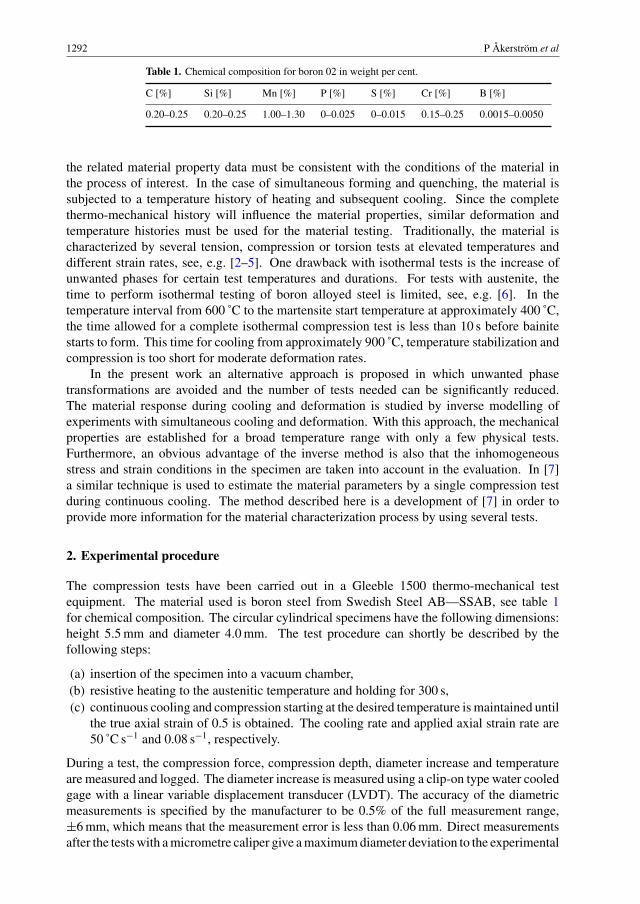
1292 P Åkerstrom et al
Table 1. Chemical composition for boron 02 in weight per cent.
C [%] Si [%] Mn [%] P [%] S [%] Cr [%] B [%]
0.20–0.25 0.20–0.25 1.00–1.30 0–0.025 0–0.015 0.15–0.25 0.0015–0.0050
the related material property data must be consistent with the conditions of the material inthe process of interest. In the case of simultaneous forming and quenching, the material issubjected to a temperature history of heating and subsequent cooling. Since the completethermo-mechanical history will influence the material properties, similar deformation andtemperature histories must be used for the material testing. Traditionally, the material ischaracterized by several tension, compression or torsion tests at elevated temperatures anddifferent strain rates, see, e.g. [2–5]. One drawback with isothermal tests is the increase ofunwanted phases for certain test temperatures and durations. For tests with austenite, thetime to perform isothermal testing of boron alloyed steel is limited, see, e.g. [6]. In thetemperature interval from 600 ˚C to the martensite start temperature at approximately 400 ˚C,the time allowed for a complete isothermal compression test is less than 10 s before bainitestarts to form. This time for cooling from approximately 900 ˚C, temperature stabilization andcompression is too short for moderate deformation rates.
In the present work an alternative approach is proposed in which unwanted phasetransformations are avoided and the number of tests needed can be significantly reduced.The material response during cooling and deformation is studied by inverse modelling ofexperiments with simultaneous cooling and deformation. With this approach, the mechanicalproperties are established for a broad temperature range with only a few physical tests.Furthermore, an obvious advantage of the inverse method is also that the inhomogeneousstress and strain conditions in the specimen are taken into account in the evaluation. In [7]a similar technique is used to estimate the material parameters by a single compression testduring continuous cooling. The method described here is a development of [7] in order toprovide more information for the material characterization process by using several tests.
2. Experimental procedure
The compression tests have been carried out in a Gleeble 1500 thermo-mechanical testequipment. The material used is boron steel from Swedish Steel AB—SSAB, see table 1for chemical composition. The circular cylindrical specimens have the following dimensions:height 5.5 mm and diameter 4.0 mm. The test procedure can shortly be described by thefollowing steps:
(a) insertion of the specimen into a vacuum chamber,(b) resistive heating to the austenitic temperature and holding for 300 s,(c) continuous cooling and compression starting at the desired temperature is maintained until
the true axial strain of 0.5 is obtained. The cooling rate and applied axial strain rate are50 ˚C s−1 and 0.08 s−1, respectively.
During a test, the compression force, compression depth, diameter increase and temperatureare measured and logged. The diameter increase is measured using a clip-on type water cooledgage with a linear variable displacement transducer (LVDT). The accuracy of the diametricmeasurements is specified by the manufacturer to be 0.5% of the full measurement range,±6 mm, which means that the measurement error is less than 0.06 mm. Direct measurementsafter the tests with a micrometre caliper give a maximum diameter deviation to the experimental

Material parameter estimation for boron steel 1293
265°C/s
25°C/s
2.5°C/s
A
M
B
FP
ΗV 10 490 465 190
800
700
600
500
400
300
200
100
Tem
p [°
C]
1 10 100 1000
Time [s]
Figure 1. CCT diagram for the boron 02 steel given in the manufacturer’s technical specification.The meaning of the letters used in the figure are as follows: A—Austenite, F—Ferrite, P—Pearlite,B—Bainite and M—Martensite. The Vickers hardness is denoted by HV.
of 0.05 mm. With the current test equipment, the diametric increase for one cross section at thetime can be measured, in this case at the specimen mid-height. The temperature is measuredusing a Pt/PtRh-thermocouple welded on the surface of the specimen (mid-height). Graphiteand tantalum foils have been used to reduce the friction and to prevent sticking between thetungsten carbide anvils and the test specimen. For the strain rate 0.08 s−1, three overlappingtemperature intervals for the compression tests have been carried out in order to providea wide range of deformation–temperature combinations. The temperature intervals for thestrain rate of 0.08 s−1 are (in degree centigrade): high—[936,630], medium—[788,481] andlow—[638,350]. Two specimens at each temperature interval have been tested, to assure thatthe obtained data are reasonable and that the deviations between the tests are small. Thecontinuous cooling diagram (CCT), which indicates the hardenability of the steel, is shown infigure 1. The diagram shows that a cooling rate of 50 ˚C s−1 would give a final microstructurecontaining only martensite.
3. Numerical procedures
The parameter estimation process is based on the inverse approach, see, e.g. [7–10]. Here theFE-method is applied to solve the equations of motions of the direct problem, see section 3.1,and an optimization algorithm is used to find a suitable set of material parameters to a modeldescribing the material hardening.
3.1. The direct problem
The direct problem consists of computing the response of the FE model, which is subjected tovariations of the parameters in a model that generates the flow stress. In the present work theexplicit FE program LS-Dyna [11] is used for solving the direct problem. An explicit simulationis accomplished without forming a stiffness matrix or solving any equations, thus reducingcore storage requirements and avoiding solution failures, see [12]. Complex geometriesin industrial applications with contact impact, large deformations, nonlinear materials and
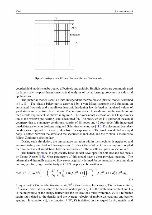
1294 P Åkerstrom et al
Anvil
Specimen
Y
X
Figure 2. Axisymmetric FE mesh that describes the Gleeble model.
coupled field models can be treated effectively and quickly. Explicit codes are commonly usedfor large scale coupled thermo-mechanical analyses of metal forming processes in industrialapplications.
The material model used is a rate independent thermo-elastic–plastic model describedin [1, 13]. The plastic behaviour is described by a von Mises isotropic yield function, anassociated flow rule and a nonlinear isotropic hardening law defined as tabulated values ofyield stress and effective plastic strain. The axisymmetric FE mesh used in the simulation ofthe Gleeble experiments is shown in figure 2. The dimensional increase of the FE specimensdue to the resistive pre-heating is not accounted for. The mesh, which is a quarter of the actualgeometry due to symmetry conditions, consist of 68 nodes and 47 four-node fully integratedquadrilateral elements (volume weighted Galerkin elements, see [11]). Displacement boundaryconditions are applied to the anvil, taken from the experiments. The anvil is modelled as a rigidbody. Contact between the anvil and the specimen is included, and the friction is assumed tofollow Coulomb’s friction law.
During each simulation, the temperature variation within the specimen is neglected andassumed to be prescribed and homogeneous. To check the validity of this assumption, coupledthermo-mechanical simulations have been conducted. The results are given in section 4.2.
The hardening model is a physically based model developed for both bcc and fcc metalsby Nemat-Nasser [14]. Most parameters of this model have a clear physical meaning. Theathermal and thermally activated flow stress originally defined for commercially pure tantalumand oxygen free, high conductivity (OFHC) copper can be written as
σy(ε, εpl, T ) = σ 0
(1 −
(−kT
G0
(ln
ε
ε0+ ln f (εpl, T )
))1/q )1/p
f (εpl, T ) + σ 0a g(εpl, dg).
(1)
In equation (1), ε is the effective strain rate, εpl is the effective plastic strain, T is the temperature,σ 0 is an effective stress value to be determined empirically, k is the Boltzman constant and G0
is the magnitude of the energy barrier that the dislocations must overcome. ε0 is a referencestrain rate related to the density and the average velocity of mobile dislocations and barrierspacing. In equation (1), the function f (εpl, T ) is defined in the sequel for fcc metals, and
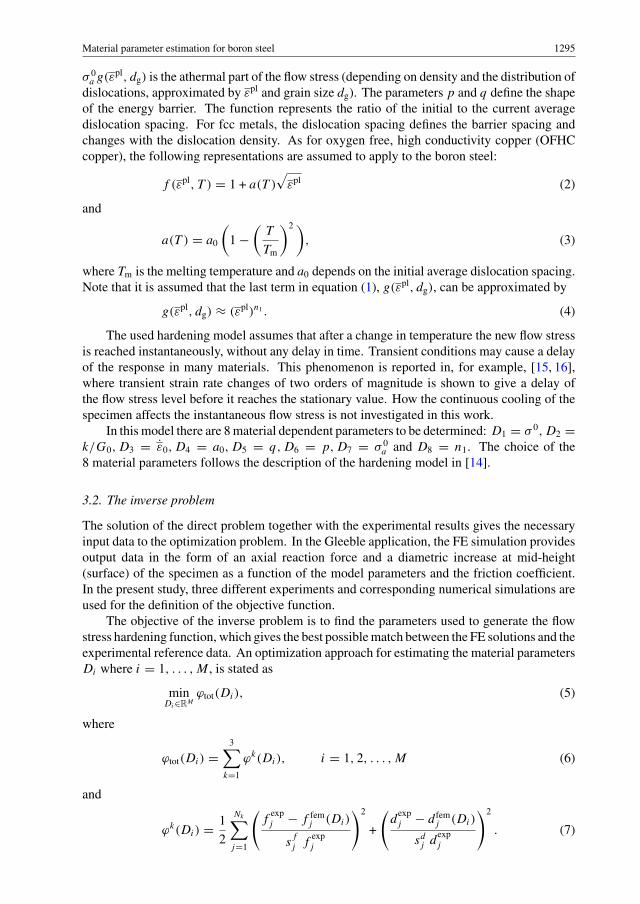
Material parameter estimation for boron steel 1295
σ 0a g(εpl, dg) is the athermal part of the flow stress (depending on density and the distribution of
dislocations, approximated by εpl and grain size dg). The parameters p and q define the shapeof the energy barrier. The function represents the ratio of the initial to the current averagedislocation spacing. For fcc metals, the dislocation spacing defines the barrier spacing andchanges with the dislocation density. As for oxygen free, high conductivity copper (OFHCcopper), the following representations are assumed to apply to the boron steel:
f (εpl, T ) = 1 + a(T )√
εpl (2)
and
a(T ) = a0
(1 −
(T
Tm
)2 ), (3)
where Tm is the melting temperature and a0 depends on the initial average dislocation spacing.Note that it is assumed that the last term in equation (1), g(εpl, dg), can be approximated by
g(εpl, dg) ≈ (εpl)n1 . (4)
The used hardening model assumes that after a change in temperature the new flow stressis reached instantaneously, without any delay in time. Transient conditions may cause a delayof the response in many materials. This phenomenon is reported in, for example, [15, 16],where transient strain rate changes of two orders of magnitude is shown to give a delay ofthe flow stress level before it reaches the stationary value. How the continuous cooling of thespecimen affects the instantaneous flow stress is not investigated in this work.
In this model there are 8 material dependent parameters to be determined: D1 = σ 0, D2 =k/G0, D3 = ε0, D4 = a0, D5 = q, D6 = p, D7 = σ 0
a and D8 = n1. The choice of the8 material parameters follows the description of the hardening model in [14].
3.2. The inverse problem
The solution of the direct problem together with the experimental results gives the necessaryinput data to the optimization problem. In the Gleeble application, the FE simulation providesoutput data in the form of an axial reaction force and a diametric increase at mid-height(surface) of the specimen as a function of the model parameters and the friction coefficient.In the present study, three different experiments and corresponding numerical simulations areused for the definition of the objective function.
The objective of the inverse problem is to find the parameters used to generate the flowstress hardening function, which gives the best possible match between the FE solutions and theexperimental reference data. An optimization approach for estimating the material parametersDi where i = 1, . . . , M , is stated as
minDi∈RM
ϕtot(Di), (5)
where
ϕtot(Di) =3∑
k=1
ϕk(Di), i = 1, 2, . . . , M (6)
and
ϕk(Di) = 1
2
Nk∑j=1
(f
expj − f fem
j (Di)
sf
j fexpj
)2
+
(d
expj − d fem
j (Di)
sdj d
expj
)2
. (7)

1296 P Åkerstrom et al
Here fexpj , f fem
j , dexpj and d fem
j are the experimental and calculated forces and diametricincreases for point j on each curve, respectively. The terms (1/f
expj ) and (1/d
expj ) are
normalization or weight factors that are applied to avoid adding terms of different orders ofmagnitude. The minimum of equation (6) gives the closest match in a least square sensebetween the Nk sample points of each FE solution and corresponding experimental data(index k is used to represent the different temperature intervals). The justification of theleast square criterion is based on the hypothesis that the sum of several different contributionswill tend to be normally distributed irrespective of the probability distribution of the individualcontributions according to the central limit theorem, see e.g. [17]. In the Gleeble tests, theuncertainties associated with the set of measurements are not known in advance, and we assumethat all measurements have the same standard deviation (sf
j = sdj = s) and that the model
fits well. Then we can proceed by first assigning an arbitrary constant value, in this casesf
j = sdj = s = 1, to all points. When the material parameters are determined by minimizing
equation (6), one can proceed by calculating the standard deviation between measured andcalculated data ([18]), see section 4.1.
In searching for the minimum value of equation (6), the subplex algorithm proposed by [19]has been used. The subplex algorithm is a direct search method for unconstrained optimization,i.e. there is no need for calculating the gradient of ϕk(Di). The subplex method is well suitedfor optimizing noisy and non-smooth objective functions. Consequently, constraints and errorhandling can rationally be implemented by means of uncomplicated penalty functions. Thefocus in this work has been on testing and evaluating models in the context of inverse analysis.There are a number of more efficient candidate algorithms available for finding local and globalminima of functions. However, the choice of optimization method here emphasizes ease ofimplementation, robustness and stability rather than computational efficiency.
The inverse problem is solved by a set of customized subprograms: analyser programs,interface processors and a connecting network. The analyser programs are the FE programwith a user defined material subroutine and the optimization software. Interface processorsare in-house programs for setting up the correct input format for each analyser program. Theconnecting network is in this case the Linux operating system, which can be programmedthrough shell programs to control the data flow and to manage the necessary datacommunication. Figure 3 shows a schematic structure for the optimization process.
3.3. Sensitivity and parameter confidence interval estimation
In this section a procedure for sensitivity and confidence interval estimation is introducedfor the different model parameters. The results can be seen in section 4.1 for the estimatedparameters with the friction coefficient 0.02. A more detailed description of the procedure canbe seen in, e.g. [20, 21].
3.3.1. Sensitivity. An indicator of the quality of the parameter estimation can be obtainedfrom the Gauss–Newton matrix, G, which is a first order approximation of the Hessian matrixfor ϕtot. The objective function for temperature interval No k can be written as
ϕk(D) = 1
2
Nk∑l=1
(r21l(D) + r2
2l(D)) = 1
2(rT
1 (D)r1(D) + rT2 (D)r2(D)), (8)
where
r1l(D) = (fexpl − f fem
l )w1l (9)
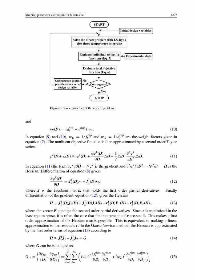
Material parameter estimation for boron steel 1297
START
Solve the direct problem with LS-Dyna(for three temperature intervals)
Evaluate individual objective functions (Eq. 7)
Evaluate total objective function (Eq. 6)
Optimization routineprovides a new set of
design variables
Experimental data
Convergence?
Yes
No
STOP
Initial design variables
Figure 3. Basic flowchart of the inverse problem.
and
r2l(D) = (dexpl − d fem
l )w2l . (10)
In equation (9) and (10), w1l = 1/fexpl and w2l = 1/d
expl are the weight factors given in
equation (7). The nonlinear objective function is then approximated by a second order Taylorseries:
ϕk(D + �D) ≈ ϕk(D) +∂ϕk(D)
∂D�D +
1
2�DT ∂2ϕk
∂D2 �D. (11)
In equation (11) the term ∂ϕk/∂D = ∇ϕk is the gradient and ∂2ϕk/∂D2 = ∇2ϕk = H is theHessian. Differentiation of equation (8) gives
∂ϕk(D)
∂D= JT
1 (D)r1 + JT2 (D)r2, (12)
where J is the Jacobian matrix that holds the first order partial derivatives. Finallydifferentiation of the gradient, equation (12), gives the Hessian
H = JT1 (D)J1(D) + JT
2 (D)J2(D) + rT1 (D)F1(D) + rT
2 (D)F2(D), (13)
where the vector F contains the second order partial derivatives. Since r is minimized in theleast square sense, it is often the case that the components of r are small. This makes a firstorder approximation of the Hessian matrix possible. This is equivalent to making a linearapproximation to the residuals r. In the Gauss-Newton method, the Hessian is approximatedby the first order terms of equation (13) according to
H ≈ JT1 J1 + JT
2 J2 = G, (14)
where G can be calculated as
Gij =⟨∂ϕtot
∂Di
,∂ϕtot
∂Dj
⟩=
3∑k=1
Nk∑l=1
((w1l)
2 ∂f feml
∂Di
∂f feml
∂Dj
+ (w2l)2 ∂d fem
l
∂Di
∂d feml
∂Dj
)k
. (15)
1298 P Åkerstrom et al
Here Nk is the number of measured points in temperature interval k. To approximate thesensitivity terms ∂f fem
l /∂Dm and ∂d feml /∂Dm the forward difference approach is applied as
∂f feml
∂Dm
≈ f feml (Dm + �Dm) − f fem
l (Dm)
�Dm
(16)
and
∂r feml
∂Dm
≈ d feml (Dm + �Dm) − d fem
l (Dm)
�Dm
. (17)
To select appropriate step sizes in equations (16) and (17), a method to determine ‘optimal’steps has been used. The procedure is described in [22, 23]. An estimation of the correlationbetween two derivatives can be calculated by
cij = cos
(∂ϕtot
∂Di
,∂ϕtot
∂Dj
)= Gij√
GiiGjj
. (18)
3.3.2. Confidence interval estimation. To estimate confidence intervals for the individualmaterial parameters, the following expressions, see [21], can be used:
I = (Dopti − t
√Vii, D
opti + t
√Vii), (19)
where the variance can be calculated as
V = [G(Dopt)]−1ϕtot(Dopt)
Ntot − M(20)
and G(Dopt) is the Gauss-Newton matrix calculated in the neighbourhood of the optimal modelparameters. Ntot is the total number of points in the measured data and t depends on theconfidence level, a 95% confidence interval gives t = 1.960.
3.4. Validation of estimated stress–strain data
To evaluate the obtained data from the optimization procedure, a separate forming experimenthas been carried out. In this section, the experiment and corresponding simulation model aredescribed. Section 4.3.1 summarizes the outcome from the validation.
3.4.1. Validation experiment. The principle of the test is to hot-form a simple hat sectionwith a conventional tool, according to figure 4, from a boron steel strip. The tool material usedis SS2242. Prior to forming, the steel strip is heated in an electrical furnace to approximately930 ˚C and kept at this temperature for 300 s. Therefore, we can expect a fully austenitizedstructure. Figure 5 shows the dimensions of the steel strip. The forming test has been carriedout in a Roell Amsler HBS500 test machine. During the test the upper tool was given a constantvelocity of 10 mm s−1. The process time, forming force, temperature and displacement wererecorded during the test. The total time to finish the forming operation was 5 s. Only theforce in the actual deformation step is of interest (but not the force when the upper tool hitsthe bottom and the final cooling and hardening take place). The temperature was measured atseveral points in the upper/lower tool and at one point on the steel strip edge as illustrated infigure 5.
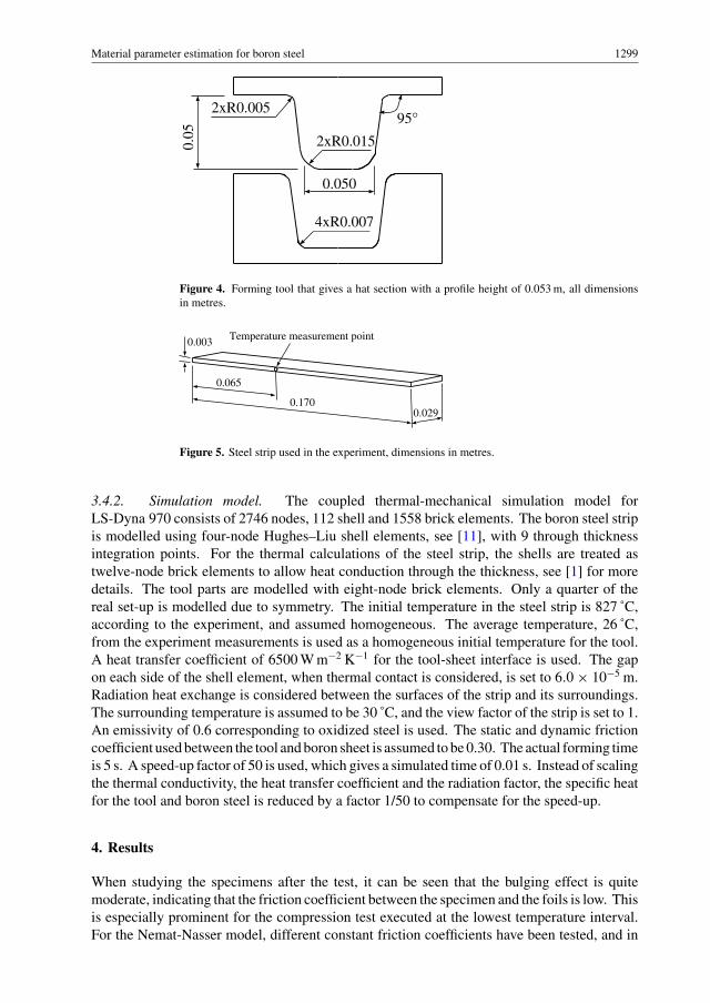
Material parameter estimation for boron steel 1299
2xR0.005
2xR0.0150.05
95°
4xR0.007
0.050
Figure 4. Forming tool that gives a hat section with a profile height of 0.053 m, all dimensionsin metres.
0.003
0.065
0.1700.029
Temperature measurement point
Figure 5. Steel strip used in the experiment, dimensions in metres.
3.4.2. Simulation model. The coupled thermal-mechanical simulation model forLS-Dyna 970 consists of 2746 nodes, 112 shell and 1558 brick elements. The boron steel stripis modelled using four-node Hughes–Liu shell elements, see [11], with 9 through thicknessintegration points. For the thermal calculations of the steel strip, the shells are treated astwelve-node brick elements to allow heat conduction through the thickness, see [1] for moredetails. The tool parts are modelled with eight-node brick elements. Only a quarter of thereal set-up is modelled due to symmetry. The initial temperature in the steel strip is 827 ˚C,according to the experiment, and assumed homogeneous. The average temperature, 26 ˚C,from the experiment measurements is used as a homogeneous initial temperature for the tool.A heat transfer coefficient of 6500 W m−2 K−1 for the tool-sheet interface is used. The gapon each side of the shell element, when thermal contact is considered, is set to 6.0 × 10⁻⁵ m.Radiation heat exchange is considered between the surfaces of the strip and its surroundings.The surrounding temperature is assumed to be 30 ˚C, and the view factor of the strip is set to 1.An emissivity of 0.6 corresponding to oxidized steel is used. The static and dynamic frictioncoefficient used between the tool and boron sheet is assumed to be 0.30. The actual forming timeis 5 s. A speed-up factor of 50 is used, which gives a simulated time of 0.01 s. Instead of scalingthe thermal conductivity, the heat transfer coefficient and the radiation factor, the specific heatfor the tool and boron steel is reduced by a factor 1/50 to compensate for the speed-up.
4. Results
When studying the specimens after the test, it can be seen that the bulging effect is quitemoderate, indicating that the friction coefficient between the specimen and the foils is low. Thisis especially prominent for the compression test executed at the lowest temperature interval.For the Nemat-Nasser model, different constant friction coefficients have been tested, and in

1300 P Åkerstrom et al
0 0.05 0.1 0.150
5
10
15
μ
Obj
ectiv
e fu
nctio
n va
lue
Figure 6. Objective function value for different friction coefficients.
one optimization run the friction coefficient has been included as a design variable. Frictionbetween the tungsten carbide anvils, tantalum foil, graphite foil and the boron specimen in thevacuum chamber at elevated temperatures is not readily obtained. The static and dynamicalfrictional coefficients are nonlinear relations, dependent on relative sliding velocity, contactpressure, temperature, atmosphere and the nature of the surfaces. In experiments performedby Boyd and Robertson [24] at high pressures (up to 2750 MPa) and with solid material aslubricants, very low friction coefficients are found. When using graphite as a lubricant [24], afriction coefficient in the interval 0.036–0.058 was obtained. During the Gleeble tests the meanpressure on the specimens contact surfaces reaches 1100 MPa. Normally at room temperatureand normal atmosphere, the friction coefficient in steel to graphite contact is near 0.1, accordingto Bowden and Tabor [25].
In the following sections the terms high, med and low are used in diagram legends tocharacterize the different temperature intervals as defined in section 2. In the FE-simulationof the Gleeble compression test, the compression time is limited to 5 s (stop temperature of389 ˚C) for the low temperature interval to avoid the influence of martensite formation duringthe cooling/compression cycle.
4.1. Nemat-Nasser model
Five different optimization runs with constant coefficients of friction (0.00, 0.04, 0.08, 0.12 and0.16) have been conducted. The objective function indicates decreasing values when reducingthe friction coefficient. Therefore, an optimization run with the friction coefficient included asan additional design variable has been conducted, resulting in a minima for μ = 0.02. Figure 6shows the objective function value as a function of the friction coefficient.
The friction and material parameters are not independent in the simulation; a variation inthe friction coefficient gives a new set of optimal material parameters (and different ‘bulging’)and therefore, different states of strain and stress within the specimen. The maximum effectiveplastic strain for the friction coefficients 0.02, 0.08 and 0.16 with corresponding optimizedparameters are 0.520, 0.616 and 0.720, respectively.
The obtained compression forces and diametric increase of the specimen for differentfriction coefficients together with experimental curves are plotted in figures 7–10. Theestimated material parameters are specified in table 2. The effect of the friction variations onthe obtained stress–strain curves is illustrated in figure 11 for the temperatures 500 and 800 ˚C.
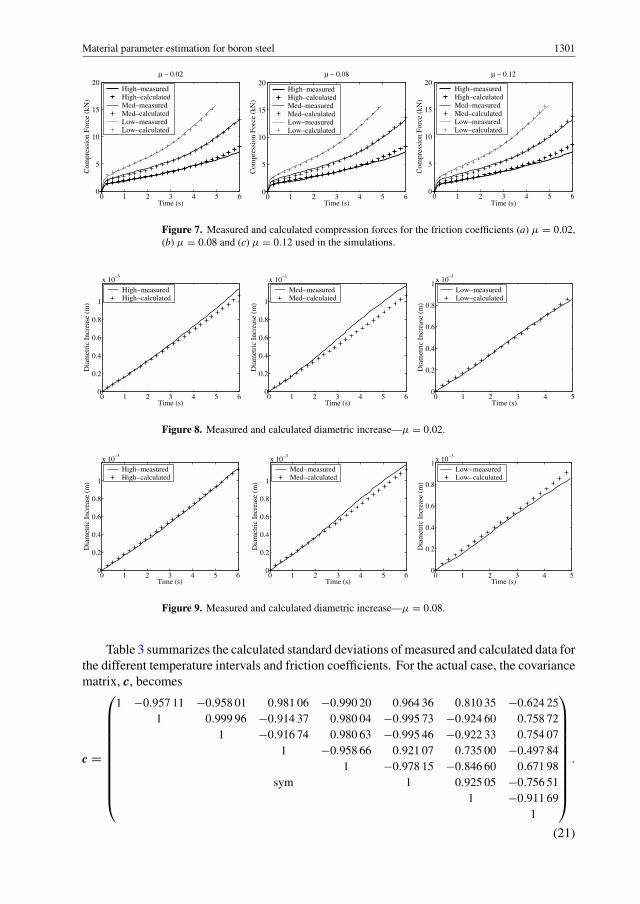
Material parameter estimation for boron steel 1301
0 1 2 3 4 5 60
5
10
15
20μ – 0.02
Time (s)
Com
pres
sion
For
ce (
kN)
High–measuredHigh–calculatedMed–measuredMed–calculatedLow–measuredLow–calculated
0 1 2 3 4 5 60
5
10
15
20μ – 0.08
Time (s)
Com
pres
sion
For
ce (
kN)
High–measuredHigh–calculatedMed–measuredMed–calculatedLow–measuredLow–calculated
0 1 2 3 4 5 60
5
10
15
20μ – 0.12
Time (s)
Com
pres
sion
For
ce (
kN)
High–measuredHigh–calculatedMed–measuredMed–calculatedLow–measuredLow–calculated
Figure 7. Measured and calculated compression forces for the friction coefficients (a) μ = 0.02,(b) μ = 0.08 and (c) μ = 0.12 used in the simulations.
0 1 2 3 4 5 60
0.2
0.4
0.6
0.8
1
x 10–3
Time (s)
Dia
met
ric
Incr
ease
(m
)
High–measuredHigh–calculated
0 1 2 3 4 50
0.2
0.4
0.6
0.8
1x 10⁻³
Time (s)
Dia
met
ric
Incr
ease
(m
)
Low–measuredLow–calculated
0 1 2 3 4 5 60
0.2
0.4
0.6
0.8
1
x 10–3
Time (s)
Dia
met
ric
Incr
ease
(m
)
Med–measuredMed–calculated
Figure 8. Measured and calculated diametric increase—μ = 0.02.
0 1 2 3 4 5 60
0.2
0.4
0.6
0.8
1
x 10–3
Time (s)
Dia
met
ric
Incr
ease
(m
)
High–measuredHigh–calculated
0 1 2 3 4 50
0.2
0.4
0.6
0.8
1x 10⁻³
Time (s)
Dia
met
ric
Incr
ease
(m
)
Low–measuredLow–calculated
0 1 2 3 4 5 60
0.2
0.4
0.6
0.8
1
x 10–3
Time (s)
Dia
met
ric
Incr
ease
(m
)
Med–measuredMed–calculated
Figure 9. Measured and calculated diametric increase—μ = 0.08.
Table 3 summarizes the calculated standard deviations of measured and calculated data forthe different temperature intervals and friction coefficients. For the actual case, the covariancematrix, c, becomes
c =
⎛⎜⎜⎜⎜⎜⎜⎜⎜⎜⎜⎝
1 −0.957 11 −0.958 01 0.981 06 −0.990 20 0.964 36 0.810 35 −0.624 251 0.999 96 −0.914 37 0.980 04 −0.995 73 −0.924 60 0.758 72
1 −0.916 74 0.980 63 −0.995 46 −0.922 33 0.754 071 −0.958 66 0.921 07 0.735 00 −0.497 84
1 −0.978 15 −0.846 60 0.671 98sym 1 0.925 05 −0.756 51
1 −0.911 691
⎞⎟⎟⎟⎟⎟⎟⎟⎟⎟⎟⎠
.
(21)

1302 P Åkerstrom et al
0 1 2 3 4 5 60
0.2
0.4
0.6
0.8
1
x 10–3
Time (s)
Dia
met
ric
Incr
ease
(m
)
High–measuredHigh–calculated
0 1 2 3 4 50
0.2
0.4
0.6
0.8
1x 10⁻³
Time (s)
Dia
met
ric
Incr
ease
(m
)
Low–measuredLow–calculated
0 1 2 3 4 5 60
0.2
0.4
0.6
0.8
1
x 10–3
Time (s)
Dia
met
ric
Incr
ease
(m
)
Med–measuredMed–calculated
Figure 10. Measured and calculated diametric increase—μ = 0.12.
Table 2. Estimated parameters for the Nemat-Nasser model.
μ 0.00 0.02 0.04 0.08 0.12 0.16
D1 = σ 0 102 [MPa] 8.445 8.885 8.396 7.483 7.760 6.818D2 = k/G0 10−5 [K−1] 1.406 1.267 1.476 1.454 1.524 1.540D3 = ε0 1010 [s−1] 2.863 0.470 3.047 2.487 2.154 3.472D4 = a0 2.405 2.310 2.622 3.059 3.029 4.028D5 = q 10−1 7.598 8.008 8.464 7.829 7.714 8.049D6 = p 10−2 7.690 6.839 10.150 8.002 7.735 8.357D7 = σ 0
a 102 [MPa] 1.574 1.375 1.478 1.916 2.325 2.482D8 = n1 10−1 1.509 1.370 1.594 2.070 2.605 2.827
0 0.1 0.2 0.3 0.4 0.50
100
200
300
400
500
600
Effective Plastic Strain
Tru
e St
ress
[M
Pa]
μ=0.04μ=0.08μ=0.12
500οC
800οC
Figure 11. Friction influence on obtained stress–strain curves for the temperatures 500 and 800 ˚C.
When an off-diagonal element (the cosines between two sensitivity vectors) is close to ±1, G isill conditioned and the confidence intervals become wide. Then the parameters in questionare linearly dependent and may be expressed in terms of each other, which means that theinfluence of two parameters on the data is similar. The three vector combinations that are most

Material parameter estimation for boron steel 1303
Table 3. Standard deviations—calculated to measured data for different friction coefficients.
Temperature interval
High Medium Low
μ sf
1 [N] sd1 10−5 [m] s
f
2 [N] sd2 10−5 [m] s
f
3 [N] sd3 10−5 [m]
0.00 267 5.25 209 9.83 158 1.320.02 279 3.57 196 8.22 157 1.330.04 329 2.21 199 6.83 147 1.950.08 387 1.39 252 4.45 146 3.810.12 463 2.87 297 2.64 222 5.610.16 534 4.38 356 1.70 324 6.89
Table 4. Estimated parameter confidence intervals (95%).
D1 ∈ (737.0, 1040.0)
D2 ∈ (−2.763 × 10⁻⁷, 2.561 × 10⁻⁵)
D3 ∈ (−1.097 × 10¹¹, 1.191 × 10¹¹)
D4 ∈ (1.842, 2.779)
D5 ∈ (0.775, 0.826)
D6 ∈ (0.063, 0.074)
D7 ∈ (122.0, 153.1)
D8 ∈ (0.113, 0.162)
closely correlated (close to ±1) are
c23 = cos
(∂ϕtot
∂D2,∂ϕtot
∂D3
)= 0.999 96,
c26 = cos
(∂ϕtot
∂D2,∂ϕtot
∂D6
)= −0.99 573,
and
c36 = cos
(∂ϕtot
∂D3,∂ϕtot
∂D6
)= −0.99 546,
where D2 = k/G0, D3 = ε0 and D6 = p according to table 2. Table 4 shows the estimatedparameter intervals.
4.2. Temperature distribution in the cylindrical specimen
Coupled thermal-mechanical simulations have been conducted to verify the validity of using ahomogeneous temperature assumption. This is shown to only affect the obtained mechanicalresponse marginally as can be seen in figure 12, making the assumption valid. In these FEsimulations the heat transfer coefficient between the anvil and specimen in combination withthe temperature of the anvil is adjusted to obtain a temperature drop close to that measured inthe experiments. The maximum temperature difference within the specimen for this case isabout 30 ˚C after 0.5 s and decreases to 10 ˚C at the end of the simulation. Similar temperaturedifferences for the other temperature intervals were obtained. Note that the 30 ˚C difference isbetween the contact interface (top/bottom surface) and the measurement point. At a depth of0.4 mm beneath the contact interface, the maximum temperature difference to the measuredtemperature is 17 ˚C, decreasing to 7 ˚C at the time 6 s. At quarter height, the maximumtemperature difference is 7 ˚C and is decreasing down to 2 ˚C at the time 6 s. A temperature

1304 P Åkerstrom et al
0 1 2 3 4 5 60
0.2
0.4
0.6
0.8
1
x 10–3
Time (s)
Dia
met
ric
Incr
ease
(m
)
Homogeneous temp.Non homogeneous temp.
0 1 2 3 4 5 60
2
4
6
8
10(a) (b)
Time (s)
Com
pres
sion
For
ce (
kN)
Homogeneous temp.Non homogeneous temp.
Figure 12. Simulations with and without homogeneous temperature in the specimen; (a) diametricincrease of specimen mid (increase from initial diameter), (b) compression force.
decrease of 7 ˚C give a rise in flow stress of 1.7% at 900 ˚C and at 600 ˚C, the corresponding riseis 2% (using equation (1) with optimized parameters). A homogeneous temperature assumptioncan therefore be further justified, because a very limited material volume is deviating intemperature more than 7 ˚C throughout the experiment. If coupled simulations were applied inthe inverse modelling, the obtained temperature history response at the specimen mid-heightis not guaranteed to follow the measured, therefore we may introduce errors greater than theabove estimated.
4.3. Strain rate effects
In this section results from Gleeble compression experiments at higher strain rates are presentedtogether with corresponding FE-simulations. The compression start temperatures correspondto those used for the reference strain rate 0.08 s−1 defined in previous sections. The naturalaxial strain rates used are 0.5 and 5.0 s−1. In corresponding simulations, the Nemat-Nassermodel was used to generate the stress–strain data, based on the estimated parameters. Theexperimentally measured temperature on each tested specimen is used in the simulation asa prescribed temperature. For the strain rate 0.5 s−1 the mean measured cooling rate is50–57 ˚C s−1. It was not possible to cool the specimens at the strain rate 5.0 s−1. Here anincrease in temperature of 1–22 ˚C as observed (the highest temperature increase for the loweststart temperature). The rise in temperature is due to plastic deformation. When the rate of heatgeneration is greater than the heat loss to the anvils and the surroundings, the temperature in thematerial increases. The material model parameters have been estimated from an experimentusing a constant strain rate of 0.08 s−1. This might be unsatisfactory from a completeness pointof view. Nevertheless, the model seems to be valid when tested using a forming simulationcase, see figure 13. The outcome of the test shows that the model with the optimized parameterset can predict the response for strain rates up to 5 s−1 with good accuracy.
4.3.1. Validation results. Figure 14 shows the measured and calculated temperature historiesin the boron steel strip. At the measurement point, the temperature drop was almost 90 ˚C duringthe forming operation, leading to a mean cooling rate of 18 ˚C s−1. The maximum mean coolingrate within the sheet reached 63 ˚C s−1. Note also that the thermal contact during the formingprocess was one-sided except when the upper tool approaches its lowest level. Computed and

Material parameter estimation for boron steel 1305
0 0.2 0.4 0.6 0.8 10
5
10
15(a) (b)
Time (s)
Com
pres
sion
For
ce (
kN)
High–measuredHigh–calculatedMed–measuredMed–calculatedLow–measuredLow–calculated
0 0.02 0.04 0.06 0.08 0.10
5
10
15
Time (s)
Com
pres
sion
For
ce (
kN)
High–measuredHigh–calculatedMed–measuredMed–calculatedLow–measuredLow–calculated
Figure 13. Measured and calculated compression forces at the true axial strain rate of (a) 0.5 s−1
and (b) 5.0 s−1.
0 1 2 3 4 5700
750
800
850
Time (s)
Tem
pera
ture
(°C
)
MeasuredCalculated
Figure 14. Measured and calculated temperature histories on the boron sheet.
measured forming forces are plotted in figure 15. Note that the global force response is in goodagreement with the experimental for the simulation with stress–strain data generated by theoptimized parameters for the Nemat-Nasser model (legend NN). For comparison purposes, asimulation with material data obtained from conventional isothermal tension tests is added tofigure 15 (legend TD). The obtained forming force in the simulation using tension test data,is at least 20% lower than the response obtained using the material data from the proposedmethod. The maximum effective plastic strain in the simulation reached 0.24 slightly belowthe upper radius. Maximum effective plastic strain at the upper and lower radius reached 0.2and 0.1, respectively.
5. Discussion and conclusions
In the current paper a methodology for estimation of material parameters for a boron steelgrade using thermo-mechanical compression experiments and inverse modelling is presented.Simultaneous cooling and compression experiments are performed instead of traditionalisothermal testing. Three different starting temperatures have been considered. The strategy
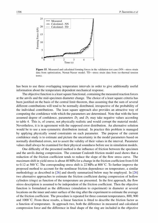
1306 P Åkerstrom et al
0 1 2 3 4 50
5
10
15
20
25
Time (s)
Form
ing
Forc
e (k
N)
MeasuredCalculated – NNCalculated – TD
Figure 15. Measured and calculated forming forces in the validation test case (NN—stress straindata from optimization, Nemat-Nasser model; TD—stress strain data from iso-thermal tensiontests).
has been to use three overlapping temperature intervals in order to give additionally usefulinformation about the temperature dependent mechanical response.
The objective function is a least square functional, containing the measured reaction forcesat the anvils and the mid-specimen diameter change. The choice of a least square criteria hasbeen justified on the basis of the central limit theorem, thus assuming that the sum of severaldifferent contributions will tend to be normally distributed, irrespective of the probability ofthe individual contributions. The least square approach also provides an attractive way ofcomputing the confidence with which the parameters are determined. Note that with the hereassumed degree of confidence, parameters D2 and D3 may take negative values accordingto table 4. This is, of course, not physically realistic and would corrupt the material model.Nevertheless, it is in agreement with the supposed error distribution. An alternative solutionwould be to use a non-symmetric distribution instead. In practice this problem is managedby applying physically sound constraints on each parameter. The purpose of the currentconfidence study is to estimate and picture the uncertainty in the model parameters based onnormally distributed errors, not to assert the validity of their values in the interval. Parametervalues shall always be examined for their physical soundness before use in simulation models.
One difficulty of the presented method is the influence of friction between the specimenand the anvils during compression. The constant Coulomb friction model used shows that areduction of the friction coefficient tends to reduce the slope of the flow stress curve. Themaximum shift in yield stress is about 40 MPa for a change in the friction coefficient from 0.04to 0.12 at 500 ˚C. The corresponding stress shift is 22 MPa at 800 ˚C. To further improve theproposed method to account for the nonlinear friction dependence on temperature, a similarmethodology as described in [26] and shortly summarized below may be employed. In [26]two alternative approaches to estimate the friction coefficient during compression of hollowcylinders (rings) as function of the temperature are presented. In the first approach, the flowstress description is assumed to be independent of the friction coefficient. Then the objectivefunction is formulated as the difference (simulation to experiment) in diameter at severallocations on the inner and outer surface of the ring after the experiment to estimate the averageof the friction coefficient. The procedure is repeated for three constant temperatures, 800, 900and 1000 ˚C. From these results, a linear function is fitted to describe the friction factor asa function of temperature. In approach two, both the difference in measured and calculatedcompression force and the difference in final shape of the ring are included in the objective
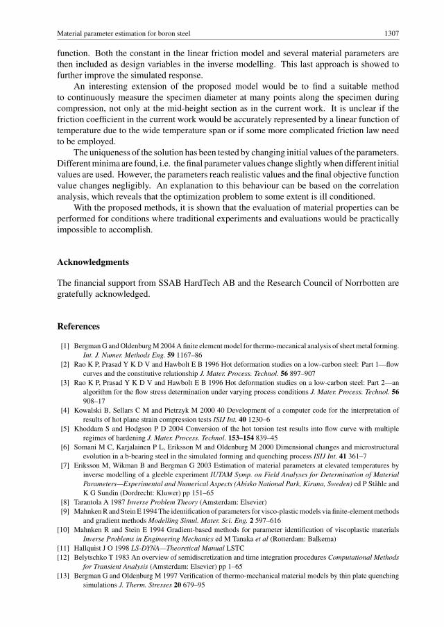
Material parameter estimation for boron steel 1307
function. Both the constant in the linear friction model and several material parameters arethen included as design variables in the inverse modelling. This last approach is showed tofurther improve the simulated response.
An interesting extension of the proposed model would be to find a suitable methodto continuously measure the specimen diameter at many points along the specimen duringcompression, not only at the mid-height section as in the current work. It is unclear if thefriction coefficient in the current work would be accurately represented by a linear function oftemperature due to the wide temperature span or if some more complicated friction law needto be employed.
The uniqueness of the solution has been tested by changing initial values of the parameters.Different minima are found, i.e. the final parameter values change slightly when different initialvalues are used. However, the parameters reach realistic values and the final objective functionvalue changes negligibly. An explanation to this behaviour can be based on the correlationanalysis, which reveals that the optimization problem to some extent is ill conditioned.
With the proposed methods, it is shown that the evaluation of material properties can beperformed for conditions where traditional experiments and evaluations would be practicallyimpossible to accomplish.
Acknowledgments
The financial support from SSAB HardTech AB and the Research Council of Norrbotten aregratefully acknowledged.
References
[1] Bergman G and Oldenburg M 2004 A finite element model for thermo-mecanical analysis of sheet metal forming.Int. J. Numer. Methods Eng. 59 1167–86
[2] Rao K P, Prasad Y K D V and Hawbolt E B 1996 Hot deformation studies on a low-carbon steel: Part 1—flowcurves and the constitutive relationship J. Mater. Process. Technol. 56 897–907
[3] Rao K P, Prasad Y K D V and Hawbolt E B 1996 Hot deformation studies on a low-carbon steel: Part 2—analgorithm for the flow stress determination under varying process conditions J. Mater. Process. Technol. 56908–17
[4] Kowalski B, Sellars C M and Pietrzyk M 2000 40 Development of a computer code for the interpretation ofresults of hot plane strain compression tests ISIJ Int. 40 1230–6
[5] Khoddam S and Hodgson P D 2004 Conversion of the hot torsion test results into flow curve with multipleregimes of hardening J. Mater. Process. Technol. 153–154 839–45
[6] Somani M C, Karjalainen P L, Eriksson M and Oldenburg M 2000 Dimensional changes and microstructuralevolution in a b-bearing steel in the simulated forming and quenching process ISIJ Int. 41 361–7
[7] Eriksson M, Wikman B and Bergman G 2003 Estimation of material parameters at elevated temperatures byinverse modelling of a gleeble experiment IUTAM Symp. on Field Analyses for Determination of MaterialParameters—Experimental and Numerical Aspects (Abisko National Park, Kiruna, Sweden) ed P Ståhle andK G Sundin (Dordrecht: Kluwer) pp 151–65
[8] Tarantola A 1987 Inverse Problem Theory (Amsterdam: Elsevier)[9] Mahnken R and Stein E 1994 The identification of parameters for visco-plastic models via finite-element methods
and gradient methods Modelling Simul. Mater. Sci. Eng. 2 597–616[10] Mahnken R and Stein E 1994 Gradient-based methods for parameter identification of viscoplastic materials
Inverse Problems in Engineering Mechanics ed M Tanaka et al (Rotterdam: Balkema)[11] Hallquist J O 1998 LS-DYNA—Theoretical Manual LSTC[12] Belytschko T 1983 An overview of semidiscretization and time integration procedures Computational Methods
for Transient Analysis (Amsterdam: Elsevier) pp 1–65[13] Bergman G and Oldenburg M 1997 Verification of thermo-mechanical material models by thin plate quenching
simulations J. Therm. Stresses 20 679–95
1308 P Åkerstrom et al
[14] Nemat-Nasser S 1999 Experimental-based micro mechanical modelling of metal plasticity with homogenisationfrom micro- to macro-scale properties IUTAM Symp. on Micro- and Macro Structural Aspects of ThermoPlasticity (Bochum, Germany) ed O T Stein and E Stein, pp 101–13
[15] Immarigeon J-P A and Jonas J J 1971 Flow stress and substructural change during the transient deformation ofarmco iron and silicon steel Acta Metall. 19 1053–61
[16] Urcola J J and Sellars C M 1987 Effect of changing strain rate on stress-strain behaviour during high temperaturedeformation Acta Metall. 35 2637–47
[17] Kreyszig E 1999 Advanced Engineering Mathemathics 8th edn (New York: Wiley)[18] Press W H and Flannery B P 1992 Numerical Recipes in Fortran 2nd edn (Cambridge: Cambridge University
Press)[19] Rowan T H 1990 Functional stability analysis of numerical algorithms Doctoral Thesis The University of Texas
at Austin, USA[20] Forestier R, Chastel Y and Massoni E 2002 3d inverse analysis model using semi-analytical differentiation
for mechanical parameter estimation 4th Int. Conf. on Inverse Problems in Engineering (Rio de Janerio,Brazil, 2002)
[21] Fletcher R 1980 Practical Methods of Optimization—Unconstrained Optimization vol 1 (New York: Wiley)[22] Iott J, Haftka R T and Adelman H M 1985 Selecting step sizes in sensitivity analysis by finite differences
Technical Memorandum 86382, NASA[23] Gill P E, Murray W and Saunders M A 1983 Computing forward-difference intervals for numerical optimization
SIAM J. Sci. Stat. Comput. 4 310–21[24] Boyd J and Robertson B P 1945 The friction properties of various lubricants at high pressures Trans. ASME 67
51–6[25] Bowden F P and Tabor D 1986 The Friction and Lubricants of Solids (Oxford: Oxford University Press)[26] Szyndler D and Pietrzyk M 2001 Identification of parameters in the internal variable constitutive model
and friction model for hot forming of steels Simulation of Materials Processing: Theory, Methods andApplications ed K-I Mori (Rotterdam: Balkema) pp 297–302

Paper C

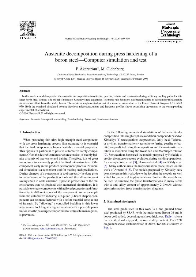
Journal of Materials Processing Technology 174 (2006) 399–406
Austenite decomposition during press hardening of aboron steel—Computer simulation and test
P. Akerstrom∗, M. OldenburgDivision of Solid Mechanics, Lulea University of Technology, SE-97187 Lulea, Sweden
Received 9 June 2004; received in revised form 15 February 2006; accepted 15 February 2006
Abstract
In this work a model to predict the austenite decomposition into ferrite, pearlite, bainite and martensite during arbitrary cooling paths for thinsheet boron steel is used. The model is based on Kirkaldy’s rate equations. The basic rate equations has been modified to account for the austenitestabilization effect from the added boron. The model is implemented as part of a material subroutine in the Finite Element Program LS-DYNA970. Both the obtained simulated volume fractions microconstituents and hardness profiles shows promising agreement to the correspondingexperimental observations.© 2006 Elsevier B.V. All rights reserved.
Keywords: Austenite decomposition modelling; Press hardening; Boron steel; Hardness estimation
1. Introduction
When producing thin ultra high strength steel componentswith the press hardening process (hot stamping) it is essentialthat the final component achieves desirable material properties.This applies in particular to passive automotive safety compo-nents. Often the desirable microstructure consists of mainly bai-nite or a mix of martensite and bainite. Therefore, it is of greatimportance to accurately predict the final microstructure of thecomponent early in the product development process. Numeri-cal simulation is a convenient tool for making such predictions.Design changes of a component or tool can easily be done priorto manufacture of the production tools and this allows to greatsavings both in costs and time. If precise predictions of the mi-crostructure can be obtained with numerical simulations, it ispossible to create components with tailored properties and func-tionality in different zones of the component. As an examplefrom the automotive industry; a b-pillar (u-beam shaped com-ponent) can be manufactured with a softer material zone at oneof its ends. By "allowing" a controlled buckling in this lowerarea, severe buckling at a higher location with a possible pene-tration into the passenger compartment at critical human regions,is prevented.
∗ Corresponding author. Tel.: +46 920 492095; fax: +46 920 491047.E-mail address: [email protected] (Akerstrom).
In the following, numerical simulations of the austenite de-composition into daughter phases and their compounds based onKirkaldys [1] rate equations are presented. Only the diffusional,or civilian, transformations (austenite to ferrite, pearlite or bai-nite) are predicted using these equations and the martensite evo-lution is modelled using the Koistinen and Marburger relation[2]. Some authors have used the models proposed by Kirkaldy topredict the micro structure evolution during welding operations,for example Watt et al. [3], Henwood et al. [4] and Oddy et al.[5]. Many authors uses the transformation model based on thework of Avrami [6–8]. The models proposed by Kirkaldy havebeen chosen in this work, due to the fact that the models are wellsuited for numerical implementations. Further, the models canbe used to simulate the phase transformations in many steelswith a total alloy content of approximately 2–3 wt.% withoutprior information from transformation diagrams.
2. Examined steel grade
The steel grade used in this work is a fine grained boronsteel produced by SSAB, with the trade name Boron 02 and ishot or cold rolled, depending on sheet thickness. Table 1 showsthe specified and a typical, measured alloy content. The CCT-diagram based on austenitization at 900 ◦C for 300 s is shown inFig. 1.
0924-0136/$ – see front matter © 2006 Elsevier B.V. All rights reserved.doi:10.1016/j.jmatprotec.2006.02.013

400 P. Akerstrom, M. Oldenburg / Journal of Materials Processing Technology 174 (2006) 399–406
Table 1Chemical composition for Boron 02 in weight percent, specified and measured
C (%) Si (%) Mn (%) P (%) S (%) Cr (%) B (ppm)
Specified 0.2–0.25 0.2–0.25 1.0–1.3 0–0.025 0–0.015 0.15–0.25 15–50Measured 0.230 0.29 1.25 0.013 0.003 0.211 30
Fig. 1. The manufacturer’s CCT diagram for the Boron 02 steel.
The initial average grain size of the hot rolled sheets used is22 �m which corresponds to an ASTM size of 8.0. The specificheat and thermal conductivity as functions of temperature for thedifferent phases used in the present work is taken from Sjostrom[9] and are not repeated here. Note that the data is for the Britishstandard steel En352 that is close to the Swedish standard steelSS2511. The main difference in chemical composition betweenthis grade and the examined one is that the boron steel do notcontain any addition of nickel (0.8–1.2 wt.% for SS2511) andthe amount chromium is lower, 0.15–0.25 compared to 0.60–1.00 wt.%. The change in enthalpy (latent heat) for the differentaustenite decomposition reactions are also taken from Sjostrom[9], and is for the ferrite, pearlite and bainite reactions equal to590 MJ/m3. For the martensite reaction the corresponding valueused, is 640 MJ/m3.
3. Tool steel
The material used in the tool parts is SS2242-02. Table 2shows the chemical composition for the steel grade. Table 3shows the specific heat and thermal conductivity as function oftemperature, from Bergman [10].
Table 2Chemical composition for the tool steel SS2242-02 given in wt.%
C (%) Si (%) Mn (%) Cr (%) Mo (%) V (%)
0.35–0.42 0.8–1.2 0.3–0.6 5.0–5.5 1.2–1.6 0.85–1.15
Table 3Heat capacity and thermal conductivity for SS2242-02
T (◦C) Cp (J/kg ◦C) k (W/m ◦C)
20 460 24.6400 460 26.2800 460 27.6
4. Experimental set-up
In this section a description of the experimental procedure will begiven. The tests are performed in an Amsler-Roell 500 machine. Thetool consists of two parts, an upper and lower part, Fig. 2. Both parts aredesigned with a 60 mm slot to achieve different cooling rates along thesheet. The hot austenitizised boron sheet is inserted between the twotools. The upper tool is given a displacement towards the lower until aforce of 126 kN is reached, and the force is maintained until the highestsheet temperature is below 60 ◦C. The magnitude of the holding forceis selected to yield a mean contact pressure of 20 MPa. The temperaturewas measured in four locations in the lower tool, Fig. 2.
The thickness of the sheets used in the tests was 3.5 mm. The tem-perature on the sheet surface is measured at two locations, Fig. 3, usingtype K thermo-couples.
Fig. 2. Plane hardening tool consisting of a upper and lower part, temperaturemeasurement points are indicated with circles, all dimensions are given in mm.
Fig. 3. Temperature measurement points on sheet surface.
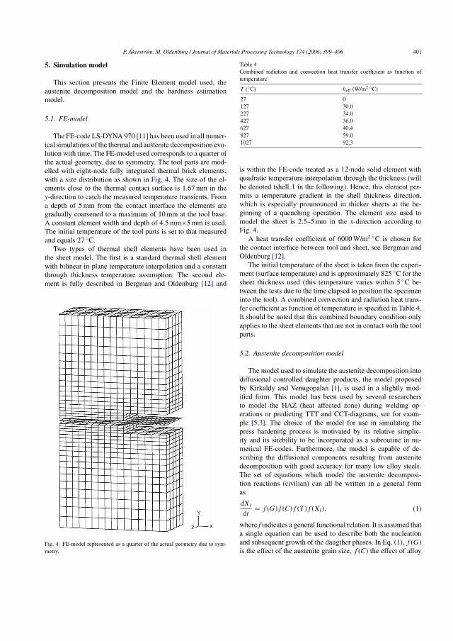
P. Akerstrom, M. Oldenburg / Journal of Materials Processing Technology 174 (2006) 399–406 401
5. Simulation model
This section presents the Finite Element model used, theaustenite decomposition model and the hardness estimationmodel.
5.1. FE-model
The FE-code LS-DYNA 970 [11] has been used in all numer-ical simulations of the thermal and austenite decomposition evo-lution with time. The FE-model used corresponds to a quarter ofthe actual geometry, due to symmetry. The tool parts are mod-elled with eight-node fully integrated thermal brick elements,with a size distribution as shown in Fig. 4. The size of the el-ements close to the thermal contact surface is 1.67 mm in they-direction to catch the measured temperature transients. Froma depth of 5 mm from the contact interface the elements aregradually coarsened to a maximum of 10 mm at the tool base.A constant element width and depth of 4.5 mm×5 mm is used.The initial temperature of the tool parts is set to that measuredand equals 27 ◦C.
Two types of thermal shell elements have been used inthe sheet model. The first is a standard thermal shell elementwith bilinear in-plane temperature interpolation and a constantthrough thickness temperature assumption. The second ele-ment is fully described in Bergman and Oldenburg [12] and
Fig. 4. FE-model represented as a quarter of the actual geometry due to sym-metry.
Table 4Combined radiation and convection heat transfer coefficient as function oftemperature
T (◦C) heff (W/m2 ◦C)
27 0127 30.0227 34.0427 36.0627 40.4827 59.01027 92.3
is within the FE-code treated as a 12-node solid element withquadratic temperature interpolation through the thickness (willbe denoted tshell 1 in the following). Hence, this element per-mits a temperature gradient in the shell thickness direction,which is especially prounounced in thicker sheets at the be-ginning of a quenching operation. The element size used tomodel the sheet is 2.5–5 mm in the x-direction according toFig. 4.
A heat transfer coefficient of 6000 W/m2 ◦C is chosen forthe contact interface between tool and sheet, see Bergman andOldenburg [12].
The initial temperature of the sheet is taken from the experi-ment (surface temperature) and is approximately 825 ◦C for thesheet thickness used (this temperature varies within 5 ◦C be-tween the tests due to the time elapsed to position the specimeninto the tool). A combined convection and radiation heat trans-fer coefficient as function of temperature is specified in Table 4.It should be noted that this combined boundary condition onlyapplies to the sheet elements that are not in contact with the toolparts.
5.2. Austenite decomposition model
The model used to simulate the austenite decomposition intodiffusional controlled daughter products, the model proposedby Kirkaldy and Venugopalan [1], is used in a slightly mod-ified form. This model has been used by several researchersto model the HAZ (heat affected zone) during welding op-erations or predicting TTT and CCT-diagrams, see for exam-ple [5,3]. The choice of the model for use in simulating thepress hardening process is motivated by its relative simplic-ity and its sitebility to be incorporated as a subroutine in nu-merical FE-codes. Furthermore, the model is capable of de-scribing the diffusional components resulting from austenitedecomposition with good accuracy for many low alloy steels.The set of equations which model the austenite decomposi-tion reactions (civilian) can all be written in a general formas
dXi
dt= f (G)f (C)f (T )f (Xi), (1)
where f indicates a general functional relation. It is assumed thata single equation can be used to describe both the nucleationand subsequent growth of the daugther phases. In Eq. (1), f (G)is the effect of the austenite grain size, f (C) the effect of alloy
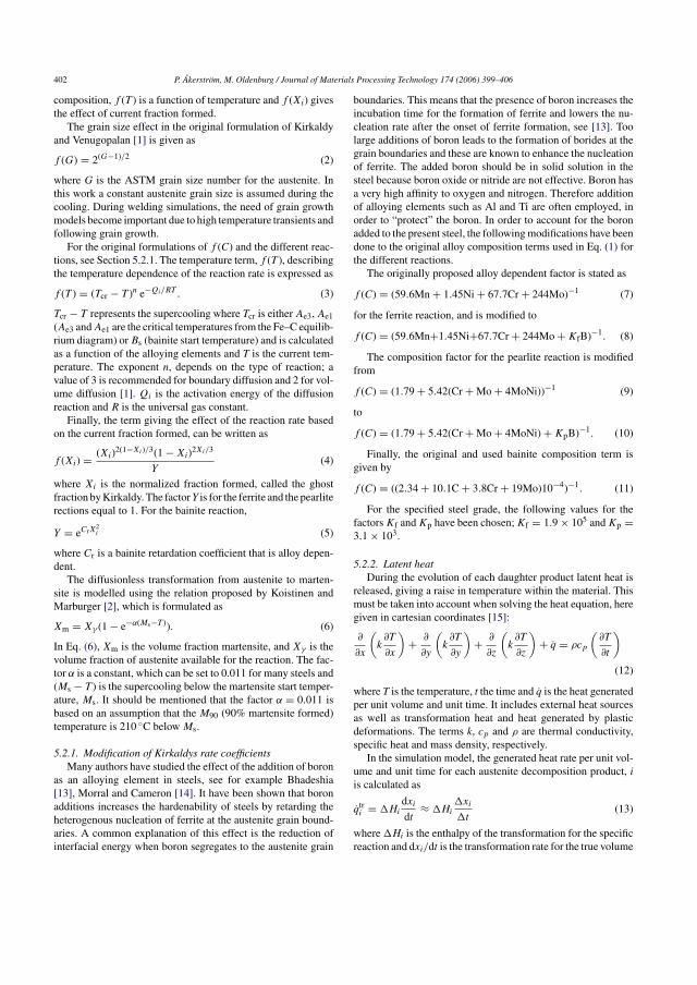
402 P. Akerstrom, M. Oldenburg / Journal of Materials Processing Technology 174 (2006) 399–406
composition, f (T ) is a function of temperature and f (Xi) givesthe effect of current fraction formed.
The grain size effect in the original formulation of Kirkaldyand Venugopalan [1] is given as
f (G) = 2(G−1)/2 (2)
where G is the ASTM grain size number for the austenite. Inthis work a constant austenite grain size is assumed during thecooling. During welding simulations, the need of grain growthmodels become important due to high temperature transients andfollowing grain growth.
For the original formulations of f (C) and the different reac-tions, see Section 5.2.1. The temperature term, f (T ), describingthe temperature dependence of the reaction rate is expressed as
f (T ) = (Tcr − T )n e−Qi/RT . (3)
Tcr − T represents the supercooling where Tcr is either Ae3, Ae1(Ae3 and Ae1 are the critical temperatures from the Fe–C equilib-rium diagram) or Bs (bainite start temperature) and is calculatedas a function of the alloying elements and T is the current tem-perature. The exponent n, depends on the type of reaction; avalue of 3 is recommended for boundary diffusion and 2 for vol-ume diffusion [1]. Qi is the activation energy of the diffusionreaction and R is the universal gas constant.
Finally, the term giving the effect of the reaction rate basedon the current fraction formed, can be written as
f (Xi) = (Xi)2(1−Xi)/3(1 − Xi)2Xi/3
Y(4)
where Xi is the normalized fraction formed, called the ghostfraction by Kirkaldy. The factor Y is for the ferrite and the pearliterections equal to 1. For the bainite reaction,
Y = eCrX2i (5)
where Cr is a bainite retardation coefficient that is alloy depen-dent.
The diffusionless transformation from austenite to marten-site is modelled using the relation proposed by Koistinen andMarburger [2], which is formulated as
Xm = Xγ (1 − e−α(Ms−T )). (6)
In Eq. (6), Xm is the volume fraction martensite, and Xγ is thevolume fraction of austenite available for the reaction. The fac-tor α is a constant, which can be set to 0.011 for many steels and(Ms − T ) is the supercooling below the martensite start temper-ature, Ms. It should be mentioned that the factor α = 0.011 isbased on an assumption that the M90 (90% martensite formed)temperature is 210 ◦C below Ms.
5.2.1. Modification of Kirkaldys rate coefficientsMany authors have studied the effect of the addition of boron
as an alloying element in steels, see for example Bhadeshia[13], Morral and Cameron [14]. It have been shown that boronadditions increases the hardenability of steels by retarding theheterogenous nucleation of ferrite at the austenite grain bound-aries. A common explanation of this effect is the reduction ofinterfacial energy when boron segregates to the austenite grain
boundaries. This means that the presence of boron increases theincubation time for the formation of ferrite and lowers the nu-cleation rate after the onset of ferrite formation, see [13]. Toolarge additions of boron leads to the formation of borides at thegrain boundaries and these are known to enhance the nucleationof ferrite. The added boron should be in solid solution in thesteel because boron oxide or nitride are not effective. Boron hasa very high affinity to oxygen and nitrogen. Therefore additionof alloying elements such as Al and Ti are often employed, inorder to “protect” the boron. In order to account for the boronadded to the present steel, the following modifications have beendone to the original alloy composition terms used in Eq. (1) forthe different reactions.
The originally proposed alloy dependent factor is stated as
f (C) = (59.6Mn + 1.45Ni + 67.7Cr + 244Mo)−1 (7)
for the ferrite reaction, and is modified to
f (C) = (59.6Mn+1.45Ni+67.7Cr + 244Mo + KfB)−1. (8)
The composition factor for the pearlite reaction is modifiedfrom
f (C) = (1.79 + 5.42(Cr + Mo + 4MoNi))−1 (9)
to
f (C) = (1.79 + 5.42(Cr + Mo + 4MoNi) + KpB)−1. (10)
Finally, the original and used bainite composition term isgiven by
f (C) = ((2.34 + 10.1C + 3.8Cr + 19Mo)10−4)−1. (11)
For the specified steel grade, the following values for thefactors Kf and Kp have been chosen; Kf = 1.9 × 10⁵ and Kp =3.1 × 10³.
5.2.2. Latent heatDuring the evolution of each daughter product latent heat is
released, giving a raise in temperature within the material. Thismust be taken into account when solving the heat equation, heregiven in cartesian coordinates [15]:
∂
∂x
(k∂T
∂x
)+ ∂
∂y
(k∂T
∂y
)+ ∂
∂z
(k∂T
∂z
)+ q = ρcp
(∂T
∂t
)(12)
where T is the temperature, t the time and q is the heat generatedper unit volume and unit time. It includes external heat sourcesas well as transformation heat and heat generated by plasticdeformations. The terms k, cp and ρ are thermal conductivity,specific heat and mass density, respectively.
In the simulation model, the generated heat rate per unit vol-ume and unit time for each austenite decomposition product, iis calculated as
qtri = �Hi
dxi
dt≈ �Hi
�xi
�t(13)
where �Hi is the enthalpy of the transformation for the specificreaction and dxi/dt is the transformation rate for the true volume
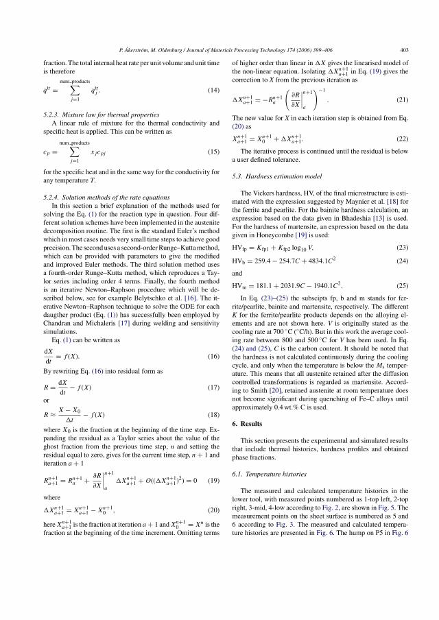
P. Akerstrom, M. Oldenburg / Journal of Materials Processing Technology 174 (2006) 399–406 403
fraction. The total internal heat rate per unit volume and unit timeis therefore
qtr =num products∑
j=1
qtrj . (14)
5.2.3. Mixture law for thermal propertiesA linear rule of mixture for the thermal conductivity and
specific heat is applied. This can be written as
cp =num products∑
j=1
xjcpj (15)
for the specific heat and in the same way for the conductivity forany temperature T.
5.2.4. Solution methods of the rate equationsIn this section a brief explanation of the methods used for
solving the Eq. (1) for the reaction type in question. Four dif-ferent solution schemes have been implemented in the austenitedecomposition routine. The first is the standard Euler’s methodwhich in most cases needs very small time steps to achieve goodprecision. The second uses a second-order Runge–Kutta method,which can be provided with parameters to give the modifiedand improved Euler methods. The third solution method usesa fourth-order Runge–Kutta method, which reproduces a Tay-lor series including order 4 terms. Finally, the fourth methodis an iterative Newton–Raphson procedure which will be de-scribed below, see for example Belytschko et al. [16]. The it-erative Newton–Raphson technique to solve the ODE for eachdaugther product (Eq. (1)) has successfully been employed byChandran and Michaleris [17] during welding and sensitivitysimulations.
Eq. (1) can be written as
dX
dt= f (X). (16)
By rewriting Eq. (16) into residual form as
R = dX
dt− f (X) (17)
or
R ≈ X − X0
�t− f (X) (18)
where X0 is the fraction at the beginning of the time step. Ex-panding the residual as a Taylor series about the value of theghost fraction from the previous time step, n and setting theresidual equal to zero, gives for the current time step, n + 1 anditeration a + 1
Rn+1a+1 = Rn+1
a + ∂R
∂X
∣∣∣∣n+1
a
�Xn+1a+1 + O((�Xn+1
a+1)2) = 0 (19)
where
�Xn+1a+1 = Xn+1
a+1 − Xn+10 , (20)
here Xn+1a+1 is the fraction at iteration a + 1 and Xn+1
0 = Xn is thefraction at the beginning of the time increment. Omitting terms
of higher order than linear in �X gives the linearised model ofthe non-linear equation. Isolating �Xn+1
a+1 in Eq. (19) gives thecorrection to X from the previous iteration as
�Xn+1a+1 = −Rn+1
a
(∂R
∂X
∣∣∣∣n+1
a
)−1
. (21)
The new value for X in each iteration step is obtained from Eq.(20) as
Xn+1a+1 = Xn+1
0 + �Xn+1a+1 . (22)
The iterative process is continued until the residual is belowa user defined tolerance.
5.3. Hardness estimation model
The Vickers hardness, HV, of the final microstructure is esti-mated with the expression suggested by Maynier et al. [18] forthe ferrite and pearlite. For the bainite hardness calculation, anexpression based on the data given in Bhadeshia [13] is used.For the hardness of martensite, an expression based on the datagiven in Honeycombe [19] is used:
HVfp = Kfp1 + Kfp2 log10 V, (23)
HVb = 259.4 − 254.7C + 4834.1C2 (24)
and
HVm = 181.1 + 2031.9C − 1940.1C2. (25)
In Eq. (23)–(25) the subscipts fp, b and m stands for fer-rite/pearlite, bainite and martensite, respectively. The differentK for the ferrite/pearlite products depends on the alloying el-ements and are not shown here. V is originally stated as thecooling rate at 700 ◦C (◦C/h). But in this work the average cool-ing rate between 800 and 500 ◦C for V has been used. In Eq.(24) and (25), C is the carbon content. It should be noted thatthe hardness is not calculated continuously during the coolingcycle, and only when the temperature is below the Ms temper-ature. This means that all austenite retained after the diffusioncontrolled transformations is regarded as martensite. Accord-ing to Smith [20], retained austenite at room temperature doesnot become significant during quenching of Fe–C alloys untilapproximately 0.4 wt.% C is used.
6. Results
This section presents the experimental and simulated resultsthat include thermal histories, hardness profiles and obtainedphase fractions.
6.1. Temperature histories
The measured and calculated temperature histories in thelower tool, with measured points numbered as 1-top left, 2-topright, 3-mid, 4-low according to Fig. 2, are shown in Fig. 5. Themeasurement points on the sheet surface is numbered as 5 and6 according to Fig. 3. The measured and calculated tempera-ture histories are presented in Fig. 6. The hump on P5 in Fig. 6
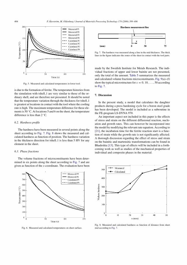
404 P. Akerstrom, M. Oldenburg / Journal of Materials Processing Technology 174 (2006) 399–406
Fig. 5. Measured and calculated temperatures in lower tool.
is due to the formation of ferrite. The temperature histories fromthe simulation with tshell 1 are very similar to those of the or-dinary shell, and are therefore not presented. It should be notedthat the temperature variation through the thickness for tshell 1is greatest at locations in contact with the tool where the coolingrate is high. The maximum temperature difference for these ele-ments is 50 ◦C. At locations 5 and 6 on the sheet, the temperaturedifference is less than 2 ◦C.
6.2. Hardness profile
The hardness have been measured in several points along thesheet according to Fig. 7. Fig. 8 shows the measured and cal-culated hardness as function of position. The hardness variationin the thickness direction for tshell 1 is less than 5 HV for anyelement in the sheet.
6.3. Phase fractions
The volume fractions of microconstituents have been deter-mined in six points along the sheet according to Fig. 7 and aregiven as function of the x-coordinate. The evaluation have been
Fig. 6. Measured and calculated temperatures on sheet surface.
Fig. 7. The hardness was measured along a line in the mid thickness. The thicklines in the figure indicates the zones of the sheet in contact with the tool parts.
made by the Swedish Institute for Metals Research. The indi-vidual fractions of upper and lower bainite are not presented,only the total of the amount. Table 5 summarizes the measuredand calculated volume fractions microconstituents. Fig. 9(a)–(f)show the typical microstructure for x = 0, 10, . . . , 50 accordingto Fig. 7.
7. Discussion
In the present study, a model that calculates the daughterproducts during a press hardening cycle for a boron steel gradehas been developed. The model is included as a subroutine inthe FE-program LS-DYNA 970.
An important aspect not included in this paper is the effectsof stress and strain on the different diffusional reaction, nucle-ation and growth rates. This can however be incorporated intothe model by modifying the relevant rate equation. According to[21], the incubation time for the ferrite reaction start is a func-tion of strain while the growth rate is not significantly affected.A thorough discussion regarding the effect of stress and strainon the bainitic and martensitic transformations can be found inBhadeshia [13]. This type of effects will be included in a forth-coming work as well as studies of the mechanical properties ofindividual and composite phases in the material.
Fig. 8. Measured and calculated hardness as function of distance from sheetmid according to Fig. 7.
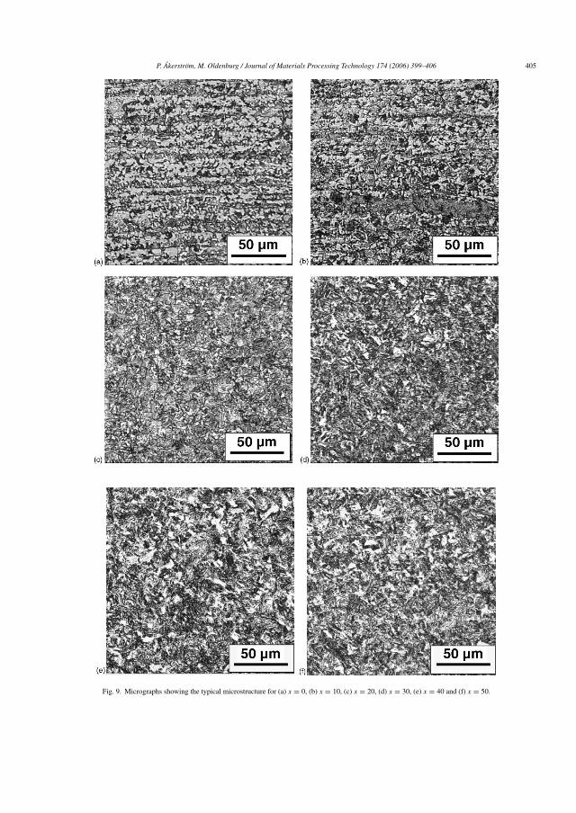
P. Akerstrom, M. Oldenburg / Journal of Materials Processing Technology 174 (2006) 399–406 405
Fig. 9. Micrographs showing the typical microstructure for (a) x = 0, (b) x = 10, (c) x = 20, (d) x = 30, (e) x = 40 and (f) x = 50.

406 P. Akerstrom, M. Oldenburg / Journal of Materials Processing Technology 174 (2006) 399–406
Table 5Measured and calculated volume fractions microconstituents obtained at specified locations
x (mm) Measured vol. fractions Calculated vol. fractions
F (%) P (%) B (%) M (%) F (%) P (%) B (%) M (%)
0 73 11 – 16 75 5 – 2010 76 9 – 15 75 10 – 1520 37 1 44 18 36 8 48 830 – – 91 9 1 – 98 140 – – 31 69 – – 58 4250 – – 26 74 – – 45 55
F: Ferrite, P: Pearlite, B: Bainite and M: Martensite.
8. Conclusions
It has been shown that the model originally proposed by[1], in a modified form that account for the addition of boron,can be used with acceptable accuracy to predict phases formedduring cooling. It is interesting to note the high fraction bai-nite found in areas of the sheet in contact with the tool. Ac-cording to the simulation, the average cooling rate in this partis as high as 170 ◦C/s (800–400 ◦C). Referring to Fig. 1, acooling rate higher than 35 ◦C/s would produce a microstruc-ture consisting of mainly martensite. To clarify this fact, fur-ther investigations need to be done. Future simulations andtests are thought to give useful insights to further improve themodel.
It is of greatest importance to include the effects of the latentheat release in the model, otherwise completely unrealistic tem-perature histories may appear, especially in areas without goodtool contact. This would certainly influence the amount and dis-tribution of the daughter phases. As a consequence, neither thecalculated specific heat nor the thermal conductivity would becorrect. A sufficiently dense mesh to ensure good contact treat-ment and heat transfer between the surfaces is crucial to achieveaccurate temperature histories. During press hardening opera-tions where the contact between sheet and tool is partially onesided, non-negligible temperature gradients through the sheetthickness may occur. Then the need for using a element able todescribe this gradient become important, not only for phase de-composition calculations but also the quench stresses and com-ponent distortion.
Acknowledgement
The financial support from SSAB HardTech AB and the Re-search Council of Norrbotten are gratefully acknowledged.
References
[1] J.S. Kirkaldy, D. Venugopalan, Prediction of microstructure and harden-ability in low alloy steels, in: A.R. Marder, J.I. Goldstein (Eds.), Interna-tional Conference on Phase Transformations in Ferrous Alloys, October1983, Philadelphia, pp. 125–148.
[2] D.P. Koistinen, R.E. Marburger, A general equation prescribing the extentof the austenite–martensite transformations in pure iron–carbon alloys andplain carbon steels, Acta Metall. 7 (1959) 59–60.
[3] D.F. Watt, L. Coon, M. Bibby, J. Goldak, C. Henwood, An algorithm formodelling microstructural development in weld heat-affected zones (parta) reaction kinetics, Acta Metall. 36 (11) (1988) 3029–3035.
[4] C. Henwood, M. Bibby, J. Goldak, D. Watt, Coupled transient heattransfer—microstructure weld computations (part b), Acta Metall. 36 (11)(1988) 3037–3046.
[5] A.S. Oddy, J.M.J. McDill, L. Karlsson, Microstructural predictions includ-ing arbitrary thermal histories, reaustenitization and carbon segregationeffects, Can. Metall. Quart. 35 (3) (1996) 275–283.
[6] M. Avrami, Kinetics of phase change. i. General theory, J. Chem. Phys. 7(1939) 1103–1112.
[7] M. Avrami, Kinetics of phase change. ii. Transformation–time relationsrandom distribution of nuclei, J. Chem. Phys. 8 (1940) 212–224.
[8] M. Avrami, Kinetics of phase change. iii. Granulation, phase change andmicrostructure, J. Chem. Phys. 9 (1941) 177–184.
[9] S. Sjostrom, The calculation of quench stresses in steel. PhD thesis,Linkoping University, 1982.
[10] G. Bergman, Modelling and Simulation of Simultaneous Forming andQuenching. PhD thesis, Lulea University of Technology, 1999.
[11] J.O. Hallquist, LS-DYNA Theoretical Manual, LSTC, 1998.[12] G. Bergman, M. Oldenburg, A finite element model for thermomechanical
analysis of sheet metal forming, Int. J. Numer. Methods Eng. 59 (9) (2004)1167–1186.
[13] B.K.D.H. Bhadeshia, Bainite in Steels. Number 504, The Institute of Ma-terials, 1992 0-901462-95-0
[14] J.E. Morral, T.B. Cameron, Boron hardenability mechanisms, in: S.K.Barenji, J.E. Morral (Eds.), Boron in Steel, AIME, Milwaukee, Wisconsin,USA, 1979, pp. 19–32.
[15] F.P. Incropera, D.P. DeWitt, Fundamentals of Heat and Mass Transfer, JohnWiley & Sons, 1990 3rd ed. 0-471-51729-1.
[16] T. Belytschko, W.K. Liu, B. Moran, Non-linear Finite Elements for Con-tinua and Structures, John Wiley & Sons Ltd., 2000 0-471-98774-3.
[17] B.G. Chandran, P. Michaleris, Prediction and optimization of microstruc-ture in material processing, Third World Congress of Structural and Mul-tidiciplinary Optimization, Buffalo, NY, 1999.
[18] Ph. Maynier, B. Jungmann, J. Dollet, Creusot-loire system for the pre-diction of the mechanical properties of low alloy steel products, in: D.V.Doane, J.S. Kirkaldy (Eds.), Hardenability Concepts with Applications toSteel, AIME, Warrendale, PA, 1978, p. 518.
[19] R.W.K. Honeycombe, Steels—Microstructure and Properties, EdvardArnold, 1981 0-7131-27937.
[20] W.F. Smith, Structure and Properties of Engineering Alloys, McGraw-Hill,1993 0-07-112829-8.
[21] S. Serajzadeh, Modelling of temperature history and phase transformationsduring cooling of steel, J. Mater. Process. Technol. 146 (2004) 311–317.

Paper D


Numerical implementation of a constitutive model
for simulation of hot stamping
P Akerstrom, G Bergman and M Oldenburg
Division of Solid Mechanics, Lulea University of Technology, SE-97187 Lulea, Sweden
E-mail: [email protected]
Abstract. In order to increase the accuracy of numerical simulations of the hotstamping process, an accurate and robust constitutive model is crucial. During theprocess, a hot blank is inserted into a tool where it is continuously formed and cooled.For the steel grades often used for this purpose, the initially austenitized blank willdecompose into different product phases depending on the cooling and mechanicalhistory. As a consequence, the phase proportions change will affect both the thermaland mechanical properties of the continuously formed and cooled blank. A thermo-elastic-plastic constitutive model based on the von Mises yield criterion with associatedplastic flow is implemented into the LS-Dyna finite element code. Models accountingfor the austenite decomposition and transformation induced plasticity are included inthe constitutive model.
The implemented model results are compared to experimental dilatation resultswith and without externally applied forces. Further, the calculated isothermalmechanical response during the formation of a new phase is compared to thecorresponding experimental response for two different temperatures.
1. Introduction
The use of ultra high strength steel components is rapidly increasing in the automotive
industry, owing to the need for higher passive safety and reduction of weight. Hot
stamping of boron alloyed steels is one technique to produce open section, ultra high
strength steel components. This manufacturing process is used in a number of vehicle
structure applications, for example side impact protection beams and bumper system
components. The prediction of the product manufacturing process and performance
requires a detailed knowledge of the material response and evolution during the
entire manufacturing process, including deformation during the fast cooling from
approximately 900 ◦C to room temperature. Coupled thermo-mechanical analysis is used
to predict the material behaviour during the hot stamping process, see e.g. Bergman and
Oldenburg [1]. To capture the residual stress state that is responsible for the distortion
of the final component, it is of great importance to capture the thermo-mechanical
history in the material model. In this work, the effort has been directed to use models
proposed in literature that make it possible to perform large scale forming simulations
including springback.
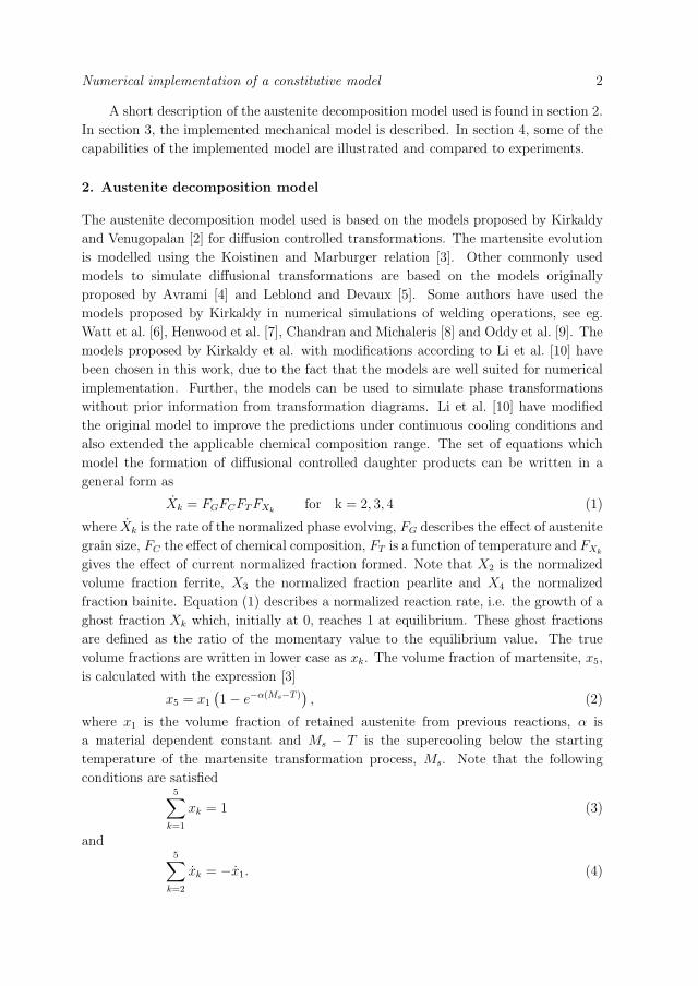
Numerical implementation of a constitutive model 2
A short description of the austenite decomposition model used is found in section 2.
In section 3, the implemented mechanical model is described. In section 4, some of the
capabilities of the implemented model are illustrated and compared to experiments.
2. Austenite decomposition model
The austenite decomposition model used is based on the models proposed by Kirkaldy
and Venugopalan [2] for diffusion controlled transformations. The martensite evolution
is modelled using the Koistinen and Marburger relation [3]. Other commonly used
models to simulate diffusional transformations are based on the models originally
proposed by Avrami [4] and Leblond and Devaux [5]. Some authors have used the
models proposed by Kirkaldy in numerical simulations of welding operations, see eg.
Watt et al. [6], Henwood et al. [7], Chandran and Michaleris [8] and Oddy et al. [9]. The
models proposed by Kirkaldy et al. with modifications according to Li et al. [10] have
been chosen in this work, due to the fact that the models are well suited for numerical
implementation. Further, the models can be used to simulate phase transformations
without prior information from transformation diagrams. Li et al. [10] have modified
the original model to improve the predictions under continuous cooling conditions and
also extended the applicable chemical composition range. The set of equations which
model the formation of diffusional controlled daughter products can be written in a
general form as
Xk = FGFCFTFXkfor k = 2, 3, 4 (1)
where Xk is the rate of the normalized phase evolving, FG describes the effect of austenite
grain size, FC the effect of chemical composition, FT is a function of temperature and FXk
gives the effect of current normalized fraction formed. Note that X2 is the normalized
volume fraction ferrite, X3 the normalized fraction pearlite and X4 the normalized
fraction bainite. Equation (1) describes a normalized reaction rate, i.e. the growth of a
ghost fraction Xk which, initially at 0, reaches 1 at equilibrium. These ghost fractions
are defined as the ratio of the momentary value to the equilibrium value. The true
volume fractions are written in lower case as xk. The volume fraction of martensite, x5,
is calculated with the expression [3]
x5 = x1
(1 − e−α(Ms−T )
), (2)
where x1 is the volume fraction of retained austenite from previous reactions, α is
a material dependent constant and Ms − T is the supercooling below the starting
temperature of the martensite transformation process, Ms. Note that the following
conditions are satisfied5∑
k=1
xk = 1 (3)
and5∑
k=2
xk = −x1. (4)
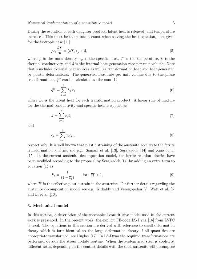
Numerical implementation of a constitutive model 3
During the evolution of each daughter product, latent heat is released, and temperature
increases. This must be taken into account when solving the heat equation, here given
for the isotropic case [11]
ρcp∂T
∂t= (kT,i), i + q, (5)
where ρ is the mass density, cp is the specific heat, T is the temperature, k is the
thermal conductivity and q is the internal heat generation rate per unit volume. Note
that q includes external heat sources as well as transformation heat and heat generated
by plastic deformations. The generated heat rate per unit volume due to the phase
transformations, qtr can be calculated as the sum [12]
qtr =5∑
k=2
Lkxk, (6)
where Lk is the latent heat for each transformation product. A linear rule of mixture
for the thermal conductivity and specific heat is applied as
k =5∑
i=1
xiki, (7)
and
cp =5∑
i=1
xicpi, (8)
respectively. It is well known that plastic straining of the austenite accelerate the ferrite
transformation kinetics, see e.g. Somani et al. [13], Serajzadeh [14] and Xiao et al.
[15]. In the current austenite decomposition model, the ferrite reaction kinetics have
been modified according to the proposal by Serajzadeh [14] by adding an extra term to
equation (1) as
Fε =1
(1 − εp1)
for εp1 < 1, (9)
where εp1 is the effective plastic strain in the austenite. For further details regarding the
austenite decomposition model see e.g. Kirkaldy and Venugopalan [2], Watt et al. [6]
and Li et al. [10].
3. Mechanical model
In this section, a description of the mechanical constitutive model used in the current
work is presented. In the present work, the explicit FE-code LS-Dyna [16] from LSTC
is used. The equations in this section are derived with reference to small deformation
theory which is form-identical to the large deformation theory if all quantities are
appropriate transformed, see Hughes [17]. In LS-Dyna the required transformations are
performed outside the stress update routine. When the austenitized steel is cooled at
different rates, depending on the contact details with the tool, austenite will decompose

Numerical implementation of a constitutive model 4
into different daughter products (or product phases). For the boron steel, the possible
daughter products are ferrite, pearlite, bainite and martensite. The morphology of
these micro structural components are very different, and consequently their mechanical
properties differ. Therefore the study of material macroscopic behaviour becomes a
difficult homogenization problem due to the fact that new phases continuously evolves
and the deformation history must be accounted for.
3.1. Constitutive model
In this model, proposed by Leblond et al. [18, 19, 20], Leblond [21] start from the
behaviour of each phase and works back to the macroscopic behaviour of the material.
The basic parts of the model will here be described for the strain hardening case. In
the original model, austenite is supposed to decompose into one product phase. In
the current treatment, it is assumed that the model is valid even for cases where the
austenite decompose into several product phases. The total increment in strain, Δεij,
is assumed to be additively decomposed and is written as
Δεij = Δεeij + Δεth
ij + Δεtrij + Δεp
ij . (10)
In equation (10), Δεeij is the elastic strain increment, Δεth
ij the thermal strain increment,
Δεtrij the isotropic transformation strain increment and Δεp
ij is the plastic strain
increment. The deviatoric stress and mean stress, respectively, corresponding to time
t+ Δt can be written as
t+Δtsij = 2t+ΔtG(
teeij + Δeij − Δεp
ij
)(11)
and
t+Δtσm = 3t+ΔtK(
tεem + Δεm − Δεth − Δεtr
), (12)
where for time t and t + Δt, t+ΔtG is the shear modulus, teeij = tsij/2
tG is the elastic
deviatoric strain, Δeij = Δεij − Δεmδij is the deviatoric strain increment, t+ΔtK is the
bulk modulus, tεem = tσm/3
tK is the mean strain, and Δεm = Δεkk/3 is the mean strain
increment.
Leblond distinguishes two cases, in which the global equivalent stress is smaller
or greater than the global uniaxial yield stress of the compound. These cases will be
treated in sections 3.1.1 and 3.1.2.
3.1.1. Global yield In the case of global yield, the von Mises yield condition for isotropic
hardening can be stated as
t+Δtf =
√3
2t+Δtsij
t+Δtsij − t+Δtσy = t+Δtσ − t+Δtσy = 0, (13)
where t+Δtσ is the von Mises effective stress and the yield stress,t+Δtσy, is supposed to
be represented by a linear mixture law as
t+Δtσy = tσy +5∑
k=1
t+Δtxkt+ΔtHkΔε
pk, (14)
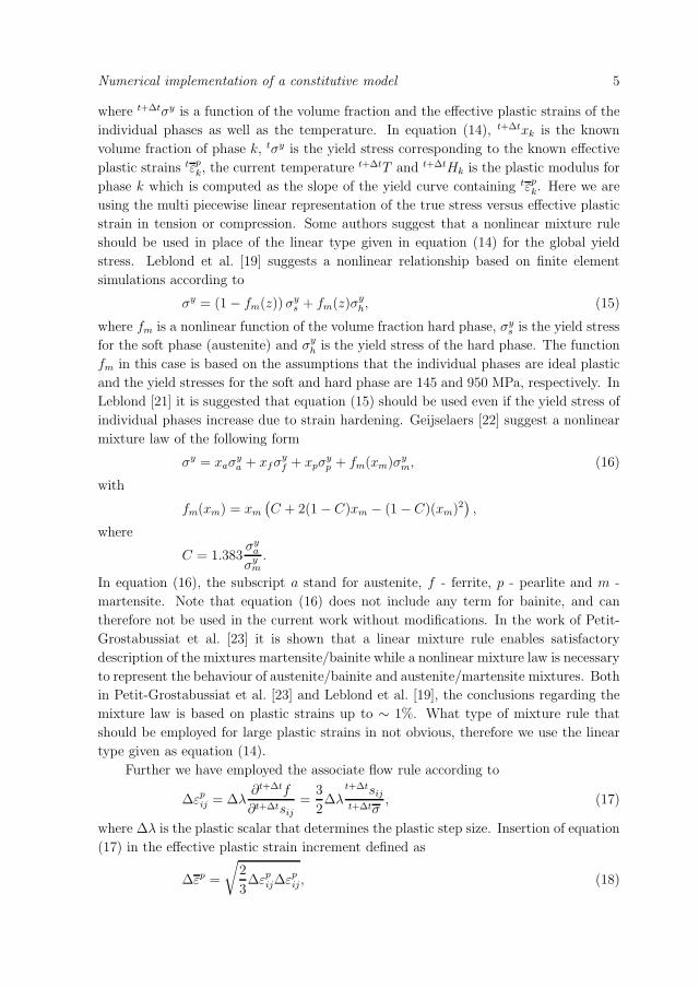
Numerical implementation of a constitutive model 5
where t+Δtσy is a function of the volume fraction and the effective plastic strains of the
individual phases as well as the temperature. In equation (14), t+Δtxk is the known
volume fraction of phase k, tσy is the yield stress corresponding to the known effective
plastic strains tεpk, the current temperature t+ΔtT and t+ΔtHk is the plastic modulus for
phase k which is computed as the slope of the yield curve containing tεpk. Here we are
using the multi piecewise linear representation of the true stress versus effective plastic
strain in tension or compression. Some authors suggest that a nonlinear mixture rule
should be used in place of the linear type given in equation (14) for the global yield
stress. Leblond et al. [19] suggests a nonlinear relationship based on finite element
simulations according to
σy = (1 − fm(z)) σys + fm(z)σy
h, (15)
where fm is a nonlinear function of the volume fraction hard phase, σys is the yield stress
for the soft phase (austenite) and σyh is the yield stress of the hard phase. The function
fm in this case is based on the assumptions that the individual phases are ideal plastic
and the yield stresses for the soft and hard phase are 145 and 950 MPa, respectively. In
Leblond [21] it is suggested that equation (15) should be used even if the yield stress of
individual phases increase due to strain hardening. Geijselaers [22] suggest a nonlinear
mixture law of the following form
σy = xaσya + xfσ
yf + xpσ
yp + fm(xm)σy
m, (16)
with
fm(xm) = xm
(C + 2(1 − C)xm − (1 − C)(xm)2
),
where
C = 1.383σy
a
σym.
In equation (16), the subscript a stand for austenite, f - ferrite, p - pearlite and m -
martensite. Note that equation (16) does not include any term for bainite, and can
therefore not be used in the current work without modifications. In the work of Petit-
Grostabussiat et al. [23] it is shown that a linear mixture rule enables satisfactory
description of the mixtures martensite/bainite while a nonlinear mixture law is necessary
to represent the behaviour of austenite/bainite and austenite/martensite mixtures. Both
in Petit-Grostabussiat et al. [23] and Leblond et al. [19], the conclusions regarding the
mixture law is based on plastic strains up to ∼ 1%. What type of mixture rule that
should be employed for large plastic strains in not obvious, therefore we use the linear
type given as equation (14).
Further we have employed the associate flow rule according to
Δεpij = Δλ
∂t+Δtf
∂t+Δtsij=
3
2Δλ
t+Δtsij
t+Δtσ, (17)
where Δλ is the plastic scalar that determines the plastic step size. Insertion of equation
(17) in the effective plastic strain increment defined as
Δεp =
√2
3Δεp
ijΔεpij , (18)

Numerical implementation of a constitutive model 6
yields
Δεp = Δλ. (19)
The radius of the von-Mises yield surface can be written as
t+ΔtR =
√2
3t+Δtσy, (20)
or
t+ΔtR =√
t+Δtsijt+Δtsij = ‖t+Δtsij‖. (21)
According to Leblond [21], the evolution equations for the internal variables is
εp
1 = εp
(22)
and
εp
k = εp − xk
xkεp
k + Θkxk
xkεp1. (23)
In equation (22) we have that the rate of the effective plastic strain in the austenite
equals the global effective strain rate. In equation (23), εp
k is the rate of the internal
variable for phase k (ferrite, pearlite, bainite or martensite). Θk is the memory
coefficient that determines the fraction of previous straining in the austenite that will
be remembered in the newly formed phase k. t+Δtεpk and t+Δtεp
1 are the current effective
plastic strain in the newly formed alpha phase and austenite, respectively. Integrating
equations (22) and (23) over a time step we obtain
Δεp1 = Δεp, (24)
and
Δεpk = Δεp + ln
(t+Δtxk
txk
) (−t+Δtεpk + Θk
t+Δtεp1
), (25)
where t+Δtεp1 and t+Δtεp
k can be written as
t+Δtεp1 = tεp
1 + Δεp1 (26)
and
t+Δtεpk = tεp
k + Δεpk. (27)
After insertion of equations (26) and (27) into equation (25), we can express Δεpk as
Δεpk =
Δεp(1 + Θkln
(t+Δtxk
txk
))1 + ln
(t+Δtxk
txk
) + ψk (28)
where
ψk =ln
(t+Δtxk
txk
)(Θk
tεp1 − tεp
k)
1 + ln(
t+Δtxktxk
) . (29)
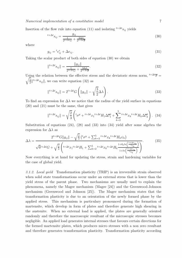
Numerical implementation of a constitutive model 7
Insertion of the flow rule into equation (11) and isolating t+Δtsij yields
t+Δtsij =gij
12t+ΔtG
+ 3Δλ2t+Δtσ
(30)
where
gij = teeij + Δeij . (31)
Taking the scalar product of both sides of equation (30) we obtain
‖t+Δtsij‖ =‖gij‖
12t+ΔtG
+ 3Δλ2t+Δtσ
. (32)
Using the relation between the effective stress and the deviatoric stress norm, t+Δtσ =√32‖t+Δtsij‖, we can write equation (32) as
‖t+Δtsij‖ = 2t+ΔtG
(‖gij‖ −
√3
2Δλ
). (33)
To find an expression for Δλ we notice that the radius of the yield surface in equations
(20) and (21) must be the same, that gives
‖t+Δtsij‖ =
√2
3
(tσy + t+Δtx1
t+ΔtH1Δεp1 +
5∑k=2
t+Δtxkt+ΔtHkΔε
pk
). (34)
Substitution of equations (24), (28) and (33) into (34) yield after some algebra the
expression for Δλ as
Δλ =2t+ΔtG‖gij‖ −
√23
(tσy +
∑5k=2
t+Δtxkt+ΔtHkψk
)√
6t+ΔtG+√
23
(t+Δtx1
t+ΔtH1 +∑5
k=2t+Δtxk
t+ΔtHk
1+θkln
„t+Δtxk
txk
«
1+ln
„t+Δtxk
txk
«) . (35)
Now everything is at hand for updating the stress, strain and hardening variables for
the case of global yield.
3.1.2. Local yield Transformation plasticity (TRIP) is an irreversible strain observed
when solid state transformations occur under an external stress that is lower than the
yield stress of the parent phase. Two mechanisms are usually used to explain the
phenomena, namely the Magee mechanism (Magee [24]) and the Greenwood-Johnson
mechanism (Greenwood and Johnson [25]). The Magee mechanism states that the
transformation plasticity is due to an orientation of the newly formed phase by the
applied stress. This mechanism is particulary pronounced during the formation of
martensite, which develop in form of plates and therefore generate high shearing in
the austenite. When no external load is applied, the plates are generally oriented
randomly and therefore the macroscopic resultant of the microscopic stresses becomes
negligible. An applied load generates internal stresses that favours certain directions for
the formed martensite plates, which produces micro stresses with a non zero resultant
and therefore generates transformation plasticity. Transformation plasticity according

Numerical implementation of a constitutive model 8
to the Greenwood-Johnson mechanism is based on the compactness difference between
the austenite and the product phase. Therefore, micro stresses are introduced that
generates plastic strains in the soft austenite when an applied deviatoric stress is applied.
If no external load is applied, no transformation plasticity is observed. This is due to
the nil volume average of the micro-plasticity. Therefore, macroscopically we can only
expect a change in volume, see e.g. Taleb et al. [26]. In the current work, the model
proposed by Leblond is used and consequently only account for the Greenwood-Johnson
mechanism, see eg. Greenwood and Johnson [25], Leblond et al. [18] and Leblond et al.
[19]. The model proposed by Leblond et al. [18] is based on the assumption that only
one product phase is formed. The transformation induced plasticity phenomenon is
often studied experimentally considering only one transformation, where in industrial
thermo-mechanical processes successive transformations generally take place in the same
material point, see e.g. Taleb and Petit [27] and cites therein. In Taleb and Petit [27]
it is shown that the volume fraction of the product phase (z) in equation (37) should
be taken as the sum of the volume fractions of the product phases, if two successive
transformations occur. In the current implementation it is assumed that all product
phases formed during applied stress, give a contribution to the plastic flow in the
austenite, as done in Sjostrom [12]. The constitutive model described in this section uses
the effective stress (ESF) algorithm proposed by Kojic and Bathe [28]. The basic idea of
the ESF algorithm is that the constitutive behaviour is written in terms of one equation
with only the effective stress as unknown variable. The solution of the unknown stress
state is reduced to find the zero of the ESF equation, as will be shown later in this
section and section 3.2. Leblond [21] gives the classical plastic flow rate, εcpij , due to the
temperature and effective stress rate as
εcpij =
3(1 − z)g(z)
2σy1(ε
p1)E
σsij +3(α1 − α2)zln(z)
σy1(ε
p1)
T sij , (36)
where z is the total amount hard phase, σy1(ε
p1) is the actual yield stress of the austenite,
g(z) is a correction factor that is introduced to account for low values of the harder phase,
E is Young’s modulus, α1 and α2 are the thermal expansion coefficient for austenite and
the harder phase, respectively. The transformation plasticity rate is given as
εtpij = −3Δεth
1−2h(
σσy
)zln(z)
σy1(ε
p1)
sij , (37)
where Δεth1−2 is the difference in compactness between austenite and the alpha based
phase, h(
σσy
)is a correction function accounting for the nonlinearity in the applied
stress, defined as
h
(σ
σy
)=
{1 if σ
σy ≤ 12
1 + 3.5(
σσy − 1
2
)if σ
σy >12,
(38)
where σy is the global yield stress according to equation (14). We can write equations
(36) and (37) as a conventional flow rule
εpij = εcp
ij + εtpij =
3
2
sij
σy1(ε
p1)ε
p. (39)
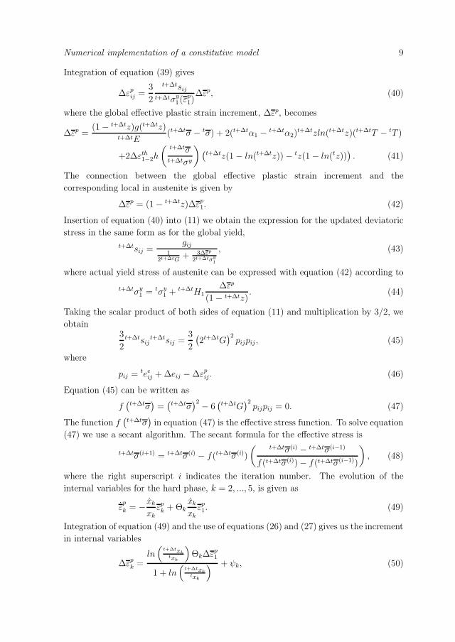
Numerical implementation of a constitutive model 9
Integration of equation (39) gives
Δεpij =
3
2
t+Δtsij
t+Δtσy1(ε
p1)
Δεp, (40)
where the global effective plastic strain increment, Δεp, becomes
Δεp =(1 − t+Δtz)g(t+Δtz)
t+ΔtE(t+Δtσ − tσ) + 2(t+Δtα1 − t+Δtα2)
t+Δtzln(t+Δtz)(t+ΔtT − tT )
+2Δεth1−2h
(t+Δtσt+Δtσy
) (t+Δtz(1 − ln(t+Δtz)) − tz(1 − ln(tz))
). (41)
The connection between the global effective plastic strain increment and the
corresponding local in austenite is given by
Δεp = (1 − t+Δtz)Δεp1. (42)
Insertion of equation (40) into (11) we obtain the expression for the updated deviatoric
stress in the same form as for the global yield,
t+Δtsij =gij
12t+ΔtG
+ 3Δεp
2t+Δtσy1
, (43)
where actual yield stress of austenite can be expressed with equation (42) according to
t+Δtσy1 = tσy
1 + t+ΔtH1Δεp
(1 − t+Δtz). (44)
Taking the scalar product of both sides of equation (11) and multiplication by 3/2, we
obtain3
2t+Δtsij
t+Δtsij =3
2
(2t+ΔtG
)2pijpij , (45)
where
pij = teeij + Δeij − Δεp
ij. (46)
Equation (45) can be written as
f(
t+Δtσ)
=(
t+Δtσ)2 − 6
(t+ΔtG
)2pijpij = 0. (47)
The function f(
t+Δtσ)
in equation (47) is the effective stress function. To solve equation
(47) we use a secant algorithm. The secant formula for the effective stress is
t+Δtσ(i+1) = t+Δtσ(i) − f(t+Δtσ(i))
(t+Δtσ(i) − t+Δtσ(i−1)
f(t+Δtσ(i)) − f(t+Δtσ(i−1))
), (48)
where the right superscript i indicates the iteration number. The evolution of the
internal variables for the hard phase, k = 2, ..., 5, is given as
εp
k = − xk
xk
εpk + Θk
xk
xk
εp1. (49)
Integration of equation (49) and the use of equations (26) and (27) gives us the increment
in internal variables
Δεpk =
ln(
t+Δtxktxk
)ΘkΔε
p1
1 + ln(
t+Δtxktxk
) + ψk, (50)
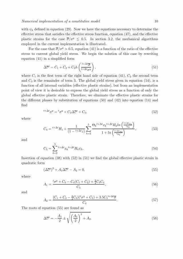
Numerical implementation of a constitutive model 10
with ψk defined in equation (29). Now we have the equations necessary to determine the
effective stress that satisfies the effective stress function, equation (47), and the effective
plastic strains for the case σ/σy ≤ 0.5. In section 3.2, the mechanical algorithms
employed in the current implementation is illustrated.
For the case that σ/σy > 0.5, equation (41) is a function of the ratio of the effective
stress to current global yield stress. We begin the solution of this case by rewriting
equation (41) in a simplified form
Δεp = C1 + C2 + C3h
(t+Δtσt+Δtσy
), (51)
where C1 is the first term of the right hand side of equation (41), C2 the second term
and C3 is the remainder of term 3. The global yield stress given in equation (14), is a
function of all internal variables (effective plastic strains), but from an implementation
point of view it is desirable to express the global yield stress as a function of only the
global effective plastic strain. Therefore, we eliminate the effective plastic strains for
the different phases by substitution of equations (50) and (42) into equation (14) and
find
t+Δtσy = tσy + C4Δεp + C5, (52)
where
C4 = t+ΔtH1 +1
(1 − t+Δtz)
5∑k=2
Θkt+Δtxk
t+ΔtHkln(
t+Δtxktxk
)1 + ln
(t+Δtxk
txk
) , (53)
and
C5 =
5∑k=2
t+Δtxkt+ΔtHkψk. (54)
Insertion of equation (38) with (52) in (51) we find the global effective plastic strain in
quadratic form
(Δεp)2 + A1Δεp − A2 = 0, (55)
where
A1 =tσy + C5 − C4(C1 + C2) + 3
4C3C4
C4
, (56)
and
A2 =(C1 + C2 − 3
4C3)(
tσy + C5) + 3.5C3t+Δtσ
C4
. (57)
The roots of equation (55) are found as
Δεp = −A1
2±
√(A1
2
)2
+ A2. (58)
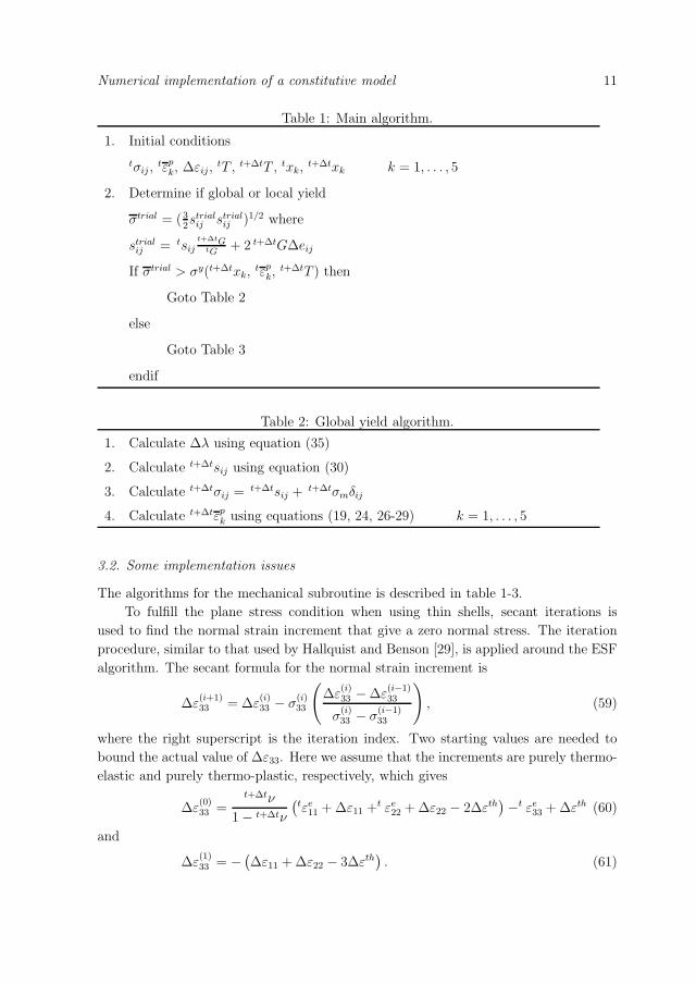
Numerical implementation of a constitutive model 11
Table 1: Main algorithm.
1. Initial conditions
tσij ,tεp
k, Δεij ,tT , t+ΔtT , txk,
t+Δtxk k = 1, . . . , 5
2. Determine if global or local yield
σtrial = (32strial
ij strialij )1/2 where
strialij = tsij
t+ΔtGtG
+ 2 t+ΔtGΔeij
If σtrial > σy(t+Δtxk,tεp
k,t+ΔtT ) then
Goto Table 2
else
Goto Table 3
endif
Table 2: Global yield algorithm.
1. Calculate Δλ using equation (35)
2. Calculate t+Δtsij using equation (30)
3. Calculate t+Δtσij = t+Δtsij + t+Δtσmδij
4. Calculate t+Δtεpk using equations (19, 24, 26-29) k = 1, . . . , 5
3.2. Some implementation issues
The algorithms for the mechanical subroutine is described in table 1-3.
To fulfill the plane stress condition when using thin shells, secant iterations is
used to find the normal strain increment that give a zero normal stress. The iteration
procedure, similar to that used by Hallquist and Benson [29], is applied around the ESF
algorithm. The secant formula for the normal strain increment is
Δε(i+1)33 = Δε
(i)33 − σ
(i)33
(Δε
(i)33 − Δε
(i−1)33
σ(i)33 − σ
(i−1)33
), (59)
where the right superscript is the iteration index. Two starting values are needed to
bound the actual value of Δε33. Here we assume that the increments are purely thermo-
elastic and purely thermo-plastic, respectively, which gives
Δε(0)33 =
t+Δtν
1 − t+Δtν
(tεe
11 + Δε11 +t εe22 + Δε22 − 2Δεth
) −t εe33 + Δεth (60)
and
Δε(1)33 = − (
Δε11 + Δε22 − 3Δεth). (61)
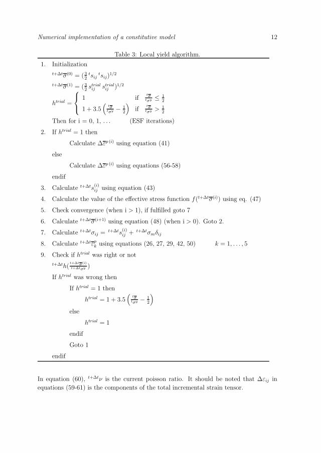
Numerical implementation of a constitutive model 12
Table 3: Local yield algorithm.
1. Initialization
t+Δtσ(0) = (32
tsijtsij)
1/2
t+Δtσ(1) = (32strial
ij strialij )1/2
htrial =
⎧⎨⎩ 1 if
tσtσy ≤ 1
2
1 + 3.5(
tσtσy − 1
2
)if
tσtσy >
12
Then for i = 0, 1, . . . (ESF iterations)
2. If htrial = 1 then
Calculate Δεp (i) using equation (41)
else
Calculate Δεp (i) using equations (56-58)
endif
3. Calculate t+Δts(i)ij using equation (43)
4. Calculate the value of the effective stress function f(t+Δtσ(i)) using eq. (47)
5. Check convergence (when i > 1), if fulfilled goto 7
6. Calculate t+Δtσ(i+1) using equation (48) (when i > 0). Goto 2.
7. Calculate t+Δtσij = t+Δts(i)ij + t+Δtσmδij
8. Calculate t+Δtεpk using equations (26, 27, 29, 42, 50) k = 1, . . . , 5
9. Check if htrial was right or not
t+Δth(t+Δtσ(i)
t+Δtσy )
If htrial was wrong then
If htrial = 1 then
htrial = 1 + 3.5(
tσtσy − 1
2
)else
htrial = 1
endif
Goto 1
endif
In equation (60), t+Δtν is the current poisson ratio. It should be noted that Δεij in
equations (59-61) is the components of the total incremental strain tensor.

Numerical implementation of a constitutive model 13
4. Validation of implemented constitutive model
In this section the response of the implemented model is compared to the corresponding
experimental results. Firstly, the calculated and measured change in diameter of a
cylindrical specimen with and without externally applied forces is compared. In these
experiments, the cooling rates have been 50 ◦C s−1. Secondly, the reaction force during
the isothermal compression of a cylindrical specimen for the temperatures 500 and 700 ◦Cis studied. These two specific temperatures have been chosen due to the fact that they
lie in a suitable interval for the actual forming stage during hot stamping. Forming thin
sheet components below 500 ◦C will lead to higher forming force as well as increased
springback.
Both the dilatational and the compression experiments have been conducted in a
Gleeble 1500 test equipment. The dimensions of the specimen used in the dilatational
experiments are; diameter 0.004 m and height 0.0055 m. The specimen dimensions
used in the isothermal compression experiments are; diameter 0.004 m and height 0.007
m. In the dilatation experiments, when an externally force is applied, it is applied
in the temperature range 600 - 500 ◦C. For further details regarding the dilatational
experiments, see Somani et al. [13]. For the isothermal compression experiments, the
thermal and mechanical histories are illustrated in figure 1. The strain rate during
the compression experiments was 0.1 s−1. The material used in all experiments is a
low alloyed steel called Boron 02 that is similar to the grade 22MnB5. The martensite
start temperature for the present steel is close to 415-420 ◦C. The flow stress data for
the different phases are extracted from; [12] and [30] for austenite, [31] and [32] for
ferrite, [12], [31] and [33] for pearlite, [23] and [31] for bainite, [34] for martensite. Data
for specific heat and thermal conductivity for each phase is taken from [12]. The value
used for the factor α in equation (2) is 0.033. The thermal expansion coefficient used for
austenite is 25·10−6 ◦C−1 and for all other constituents 11.1·10−6 ◦C−1. The compactness
difference, Δεth1−2, for the austenite to martensite reaction has been set to 6.0 · 10−3 and
for all others to 4.33 · 10−3 based on the experiments performed in [13].
The FE-model used is one eight of the actual geometry due to symmetry. It consist
of 135 eight node brick elements. For the compression case, the anvil is modelled as rigid
with 48 brick elements. In the FE-simulations, the nodal temperatures are prescribed
to follow the experimentally measured temperature. All FE-simulations are performed
with the commercial FE-code LS-Dyna [16], with the models described in the previous
sections implemented as user defined subroutines.
4.1. Dilatation results
Figure 2 show the measured and calculated diameter change as a function of the
temperature and applied force.
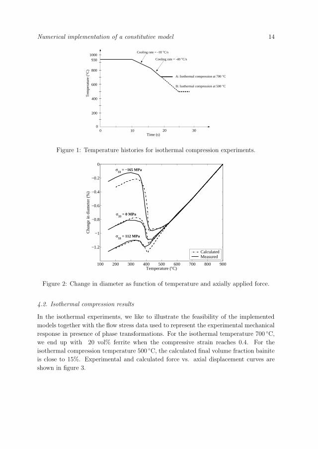
Numerical implementation of a constitutive model 14
200
400
600
800
1000
Tem
pera
ture
(°C
)
Time (s)10 20 30
Cooling rate = -18 °C/s
Cooling rate = -40 °C/s
0
A: Isothermal compression at 700 °C
B: Isothermal compression at 500 °C
0
930
Figure 1: Temperature histories for isothermal compression experiments.
100 200 300 400 500 600 700 800 900
−1.2
−1
−0.8
−0.6
−0.4
−0.2
0
Temperature (°C)
Cha
nge
in d
iam
eter
(%
)
CalculatedMeasured
σ33
= −165 MPa
σ33
= 0 MPa
σ33
= 112 MPa
Figure 2: Change in diameter as function of temperature and axially applied force.
4.2. Isothermal compression results
In the isothermal experiments, we like to illustrate the feasibility of the implemented
models together with the flow stress data used to represent the experimental mechanical
response in presence of phase transformations. For the isothermal temperature 700 ◦C,
we end up with 20 vol% ferrite when the compressive strain reaches 0.4. For the
isothermal compression temperature 500 ◦C, the calculated final volume fraction bainite
is close to 15%. Experimental and calculated force vs. axial displacement curves are
shown in figure 3.

Numerical implementation of a constitutive model 15
0 0.5 1 1.5 2
x 10−3
0
2
4
6
8
10
12
Axial displacement (m)
Com
pres
sion
for
ce (
kN)
CalculatedMeasured
500 °C
700 °C
Figure 3: Compression force versus axial displacement at the isothermal temperatures
500 and 700 ◦C.
5. Discussion
In figure 2, it can be seen that the calculated change in diameter of the specimen
follow the measured with adequate accuracy. The calculated change in diameter for
the compressive load (-165 MPa) is to low which can be explained by the fact that
somewhat to high yield stress and/or hardening for austenite for temperatures close to
400 ◦C are used. Note the deviation of the loaded dilatation curves from the unloaded
(550 - 420 ◦C), which can be explained by the fact that a small amount of bainite is
formed (∼5% in the simulations) simultaneous to the loading, then we obtain TRIP,
starting at this higher temperature. If only the martensite should form, we should only
obtain TRIP due to this reaction, starting at 420 ◦C.
As can be seen in figure 3, the calculated response are in acceptable agreement to
the experimental. For the compression at 500 ◦C, it can be observed that the used stress-
strain data seems to have to high initial yield stress and somewhat to low hardening.
The maximum difference in force level for the calculated and measured are less than
12%. These results are thus regarded as accurate enough for engineering applications.
6. Conclusions
In the current paper, a numerical implementation of a mechanical constitutive model
for simulation of hot stamping is presented. The constitutive model in combination
with the austenite decomposition model used are aimed to give product developers a
useful tool to predict formability as well as shape accuracy and springback for thermo-
mechanically formed thin sheet components. In order to further evaluate the predictive
capabilities of the implemented models, additional experiments for different thermo-
Numerical implementation of a constitutive model 16
mechanical loading histories must be conducted. The mechanical response in the model
is based on data from several different sources. Some experimental data for austenite
and martensite are reported in recent papers by the present authors. However, for
the other phases, the mechanical data found in the literature are somewhat incomplete
with respect to the temperature and strain range found in the hot stamping process.
Thus, there is a need for more thorough studies of the mechanical response of individual
phases. These studies should include evaluation of nonlinear mixture rules that may be
useful in describing the global mechanical response.
7. Acknowledgments
The financial support from Gestamp HardTech AB and the Research Council of
Norrbotten are gratefully acknowledged.

REFERENCES 17
References
[1] G. Bergman and M. Oldenburg. A finite element model for thermomechanical
analysis of sheet metal forming. Int. J. Numer. Meth. Engng., 59:1167–1186, 2004.
[2] J.S. Kirkaldy and D. Venugopalan. Prediction of microstructure and hardenability
in low alloy steels. In A.R. Marder and J.I. Goldstein, editors, Int. conference on
phase transformations in ferrous alloys, pages 125–148, Philadelphia, Oct. 1983.
[3] D.P. Koistinen and R.E. Marburger. A general equation prescribing the extent
of the austenite-martensite transformations in pure iron-carbon alloys and plain
carbon steels. Acta Metallurgica, 7:59–60, 1959.
[4] M. Avrami. Kinetics of phase change 1: general theory. J. Chem. Phys., 7:1103–
1112, 1939.
[5] J.B. Leblond and J. Devaux. A new kinetic model for anisothermal metallurgical
transformations in steels including effect of austenite grain size. Acta Metallurgica,
32:137–146, 1984.
[6] D. Watt, L. Coon, M. Bibby, J. Goldak, and C. Henwood. An algorithm for
modelling microstructural development in weld heat-affected zones (part a) reaction
kinetics. Acta Metallurgica, 36(11):3029–3035, 1988.
[7] C. Henwood, M. Bibby, J. Goldak, and D. Watt. Coupled transient heat transfer -
microstructure weld computations (part b). Acta Metallurgica, 36(11):3037–3046,
1988.
[8] B.G. Chandran and P. Michaleris. Prediction and optimization of microstructure in
material processing. In 3rd world congress of multidiciplinary optimization, Buffalo,
NY, 1999.
[9] A.S. Oddy, J.M.J. McDill, and L. Karlsson. Microstructural predictions including
arbitrary thermal histories, reaustenitization and carbon segregation effects.
Canadian Metallurgical Quartely, 35(3):275–283, 1996.
[10] M.V. Li, D.V. Niebuhr, L.L. Meekisho, and D.G. Atteridge. A computational model
for the prediction of steel hardenability. Metallurgical and Materials Transactions,
29B(3):661–672, June 1998.
[11] Y.C. Fung and P. Tong. Classical and computational solid mechanics, volume 1.
World Scientific Publishing Co. Pte. Ltd., 2001. ISBN 981-02-3912-2.
[12] S. Sjostrom. The calculation of quench stresses in steel. PhD thesis, Linkoping
University, Linkoping Sweden, 1982.
[13] M.C. Somani, L.P. Karjalainen, M. Eriksson, and M. Oldenburg. Dimensional
changes and microstructural evolution in a b-bearing steel in the simulated forming
and quenching process. ISIJ International, 41(4):361–367, 2001.
[14] S. Serajzadeh. Modelling of temperature history and phase transformations during
cooling of steel. Journal of Materials Science and Engineering, 146:311–317, 2004.
REFERENCES 18
[15] N. Xiao, M. Tong, Y. Lan, D. Li, and Y. Li. Coupled simulation of the
influence of austenita deformation on the subsequent isothermal austenite-ferrite
transformation. Acta Materialia, 54:1265–1278, March 2006.
[16] J.O. Hallquist. LS-Dyna - Theoretical manual. LSTC, Nov 2005.
[17] T.J.R. Hughes. Numerical implementation of constitutive models: rate-
independent deviatoric plasticity. In S. Nemat-Nasser et al., editor, Theoretical
Foundation for Large-scale Computations for Nonlinear Material Behaviour, pages
29–57, The Netherlands, 1984. Martinus Nijhoff.
[18] J.B. Leblond, G. Mottet, and J.C. Devaux. A theoretical and numerical approach to
the plastic behaviour of steels during phase transformations-i. derivation of general
relations. J. Mech. Phys. Solids, 34(4):395–409, 1986.
[19] J.B. Leblond, G. Mottet, and J.C. Devaux. A theoretical and numerical approach
to the plastic behaviour of steels during phase transformations-ii. study of classical
plasticity for ideal-plastic phases. J. Mech. Phys. Solids, 34(4):411–432, 1986.
[20] J.B. Leblond, J. Devaux, and J.C. Devaux. Mathematical modelling of
transformation plasticity in steels i: Case of ideal-plastic phases. International
Journal of Plasticity, 5:551–572, 1989.
[21] J.B. Leblond. Mathematical modelling of transformation plasticity in steels ii:
Coupling with strain hardening phenomena. International Journal of Plasticity, 5:
573–591, 1989.
[22] H.J.M. Geijselaers. Numerical simulation of stresses due to solid state
transformations: The simulation of laser hardening. PhD thesis, University of
Twente, Twente Enschede The Netherlands, 2003.
[23] S. Petit-Grostabussiat, L. Taleb, and J-F. Jullien. Experimental results on classical
plasticity of steels subjected to structural transformations. International Journal
of Plasticity, 20:1371–1386, 2004.
[24] C.L. Magee. Transformation kinetics, microplasticity and ageing of martensite in
Fe-31-Ni. PhD thesis, Carnegie Institute of Technologie University, Pittsburgh,
PA, 1966.
[25] G. W. Greenwood and R. H. Johnson. The deformation of metals under small
stresses during phase transformations. volume 283, pages 403–422. Proc. Royal
Society, 1965.
[26] L. Taleb, N. Cavallo, and F. Waeckel. Experimental analysis of transformation
plasticity. International Journal of Plasticity, 17:1–20, 2001.
[27] L. Taleb and S. Petit. New investigations on transformation induced plasticity
and its interactions with classical plasticity. International Journal of Plasticity, 22:
110–130, 2006.
[28] M. Kojic and K-J. Bathe. The ’effective-stress-function’ algorithm for thermo-
elasto-plasticity and creep. International Journal for Numerical Methods in
Engineering, 24:1509–1532, 1987.
REFERENCES 19
[29] J.O. Hallquist and D.J. Benson. A comparison of an explicit implementation of
the hughes-liu shell. In T.J.R. Hughes et al., editor, Finite Element Methods for
Plate and Shell Structures, Element Technology, volume 1, pages 394–431. Pineridge
Press Limited: U.K., 1986.
[30] P. Akerstrom, B. Wikman, and M. Oldenburg. Material parameter estimation for
boron steel from simultaneous cooling and compression experiments. Modelling
Simul. Mater. Sci. Eng., 13:1291–1308, 2005.
[31] Rudiono and Y. Tomota. Application of the secant method to prediction of flow
curves in multi-microstructure steels. Acta. mater., 45(5):1923–1929, 1997.
[32] C. Huang, E.B. Hawbolt, X. Chen, T.R. Meadowcroft, and D.K. Matlock. Flow
stress modeling and warm rolling simulation behavior of two ti-nb interstitial-free
steels in the ferrite region. Acta mater., 49:1445–1452, 2001.
[33] R. Nakkalil, J.R. Hornaday Jr., and M. Nabil Bassim. Characterization of the
compression properties of rail steels at high temperatures and strain rates. Materials
Science and Engineering, A141:247–260, 1991.
[34] M. Eriksson, M. Oldenburg, M.C. Somani, and L.P. Karjalainen. Testing and
evaluation of material data for analysis of forming and hardening of boron steel
components. Modelling Simul. Mater. Sci. Eng., 10:1–18, 2002.


Paper E

Numerical simulation of a thermo-mechanical sheet
metal forming experiment
P Akerstrom and M Oldenburg
Division of Solid Mechanics, Lulea University of Technology, SE-97187 Lulea, Sweden
E-mail: [email protected]
Abstract. In the design of hot stamped parts, which are subject to both internaland external constraints, it is of great importance to be able to predict the finalshape of the component as well as the hardness and thickness distribution. It isalso important to be able to predict the material state at each point of a componentbefore consideration of the final design of the part itself and the tools. In the presentwork a model for simulation of the forming and hardening phase in the hot stampingprocess is evaluated. The model is used in coupled thermo-mechanical simulationsand accounts for the effects of micro-structural changes in the material as well asclassical and transformation induced plasticity. The model is evaluated by comparingresults from a simulation with a hot stamping experiment. The experimental andthe numerically obtained forming force, final hardness, thickness and shape of the hotstamped component are compared. The evaluation shows that the most importantprocesses taking place during the thermo-mechanical process are accounted for andthat the results from the simulation are accurate enough to significantly improve theability to use simulations as a predictive tool in product development of hot stampedparts.
1. Introduction
In this paper, FE-simulation results of the hot stamping process (forming stage)
producing a component is compared to the corresponding experimental results. The
main focus is to compare the obtained final shape, hardness and thickness distribution
of the component. Traditionally when simulating the hot stamping process, the forming
stage is often simplified by assuming isothermal conditions. In other words, no heat
transfer between the workpiece and the environment and the tools are accounted for
during the forming process. Therefore, models describing the decomposition of the
initially austenitized workpiece into different product phases are not used in these cases.
In the work by Bergman and Oldenburg [1] and Wu et al. [2], the heat transfer between
the workpiece and the tool is accounted for, but the cooling rate for all material points
are assumed to be sufficiently high so the only product phase formed is martensite. In
practical hot stamping operations with the steel grades commonly used, austenite may
decompose into several product phases such as; ferrite, pearlite, bainite and martensite
depending on the temperature and stress/strain history. The continuous growth of

Thermo-mechanical sheet metal forming 2
different micro constitutients in the material affects both the thermal and mechanical
properties. In the current work, the rate equations given originally by Kirkaldy and
Venugopalan [3] with the modifications proposed by Li et al. [4] are used for the
description of the austenite decomposition into product phases. The overall logics for
the austenite decomposition model during the cooling phase follow the algorithm given
in Watt et al. [5].
The mechanical constitutive model used is an extension of the original model
proposed by Leblond et al. [6, 7, 8], Leblond [9] to treat successive transformations,
where a detailed description of the model can be found in Akerstrom et al. [10].
In section 2, a description of the experimental tools and corresponding FE-model is
presented. Section 3 is used to describe the blank and the corresponding FE-model. In
section 4, the experimental equipment used is described. In section 5, the experimental
and simulated component are compared regarding forming force, hardness and thickness
distribution as well as final component shape.
2. Tools
In this section a description of the experimental tools as well as the corresponding
FE-model is presented.
2.1. Experimental tools
The tool consists of two main parts, an upper punch and a lower die as illustrated
in figure 1. The tools will produce a component with a hat section with a height of
0.052 m (length 0.140 m), that after a transition zone (0.080 m) becomes flat (0.030
m), as can be seen in figure 1. The final length of the component is ∼0.250 m. Also,
as seen in figure 1, some additional components are added to the die. Two additional
guiding pins (φ0.01m) are used to guide the blank into the correct position in the tool.
Further, four small spring supported pins (φ0.004m) are mounted at the top of the die
to prevent the hot blank to come into tool contact during the blank insertion phase.
The temperature is measured at three locations in the lower and upper tools using
type K thermocouples, according to figure 2. The thermoelements are of insert type
with a diameter of 1.5·10−3m. The thermoelements are inserted into holes in the tools
with diameter 1.6·10−3m and the depth 20.0·10−3m. The material used in the tools is
SS2242-02, manufactured by Uddeholm AB [11]. The specific heat capacity, cp, and the
thermal conductivity, k, for the material in the hardened state are given in table 1.
Table 1: Heat capacity and thermal conductivity for SS 2242-02, from [11] and [12].
T[ ◦C] cp[J/kg ◦C] k[W/m ◦C]
20 460 25
400 460 29
600 460 30

Thermo-mechanical sheet metal forming 3
Figure 1: Illustration of tools and the shape of the final component.
0.0250.004
0.077
0.004 A
B
0.004
0.050
C
Upper tool
Lower tool
0.0500.10
0.170
0.050
83°
0.040
4×R0.005
4×R0.007
Figure 2: Location of the temperature measurement points are indicated as circles on
tool parts. All dimensions in meters.
2.2. FE-model of the tools
The 3D finite element mesh of the tool parts consists of a total of 57399 eight node brick
elements. Due to symmetry, only half of the tools are modelled. To correctly capture
the thermal contact between the hot blank and the cold tool surface, the element size
(inward the tools) closest to the tool surface is less than 1 mm. To get an accurate
representation of the curvatures of the tool radius, 5-8 elements are used to represent
it. From the mechanical point of view, the tool steel is regarded as rigid but for the
thermal analysis the data given in table 1 are used.

Thermo-mechanical sheet metal forming 4
3. Blank
This section presents the geometry of the blank and the material used, followed by a
description of the corresponding FE-model.
3.1. Experimental blank
The main dimensions of the blank used in the experiment are illustrated in figure 3,
where the thickness is 2.0 mm. The material used is a low alloyed steel (Boron02) with
the actual and specified chemical composition given in table 2.
0.168
0.14
00.
180
0.22
0
0.25
3
0.025
0.090
0.015
0.134
0.126
0.125
φ0.0102
φ0.0102
Figure 3: Dimensions of blank used in the thermo-mechanical forming experiment, all
dimensions are given in meters.
Table 2: Specified and actual chemical composition for the Boron02 steel (similar to
22MnB5) given in wt%.
C[%] Si[%] Mn[%] Cr[%] P[%] S[%] B[%] Fe[%]
Specified 0.2-0.25 0.2-0.35 1.0-1.3 0.15-0.25 <0.025 <0.015 0.0015-0.0050 bal.
Actual 0.248 0.29 1.23 0.24 0.015 0.004 0.0025 bal.
3.2. FE-model of blank
The corresponding FE-model is one half of the actual geometry due to symmetry. The
nominal size of the shell elements used to model the blank is 2.5 mm. A total of 3500

Thermo-mechanical sheet metal forming 5
Belytschko-Tsay shell elements with 5 through thickness integration points are used. For
the thermal calculations of the blank, the shells are treated as 12-node brick elements
to allow heat conduction through the thickness, see Bergman and Oldenburg [1]. The
initial dimensions of the blank according to figure 3 are increased 1% to account for the
thermal expansion due to heating. To find a good estimate for the initial temperature
to be used in the FE-simulation, a thermocouple is welded to the blank edge. The flow
stress data for the different phases is extracted from; [13] and [14] for austenite, [15] and
[16] for ferrite, [14], [15] and [17] for pearlite, [15] and [18] for bainite, [19] for martensite.
Data for thermal conductivity and specific heat for individual phases are extracted from
Sjostrom [14]. Values for the latent heat release for the formation of product phases
are; 640 · 106 J/m3 for the austenite to martensite reaction and 590 · 106 J/m3 for all
others, which are the values given in [14]. The thermal expansion coefficient used for
austenite is 25·10−6 ◦C−1 and for all other constituents 11.1·10−6 ◦C−1. The compactness
difference for the austenite to martensite reaction has been set to 6.0 · 10−3 and for all
others to 4.33 · 10−3 based on the experiments performed in [20]. For plastic strain,
no memory effects are assumed, except for the bainite transformation, as suggested in
Petit-Grostabussiat et al. [18].
4. Test equipment
The tools are mounted into a Zwick-Roell test equipment capable of precise control of
stroke and forming force, illustrated in figure 4. In the experiment, the upper punch is
given a prescribed velocity towards the die of 0.025 ms−1 and is limited to a force level of
250 kN at the end of the stroke when the hot formed component is in the actual cooling
stage. This force level is maintained until the formed component is below 100 ◦C.
4.1. Some simulation issues
In the coupled thermo-mechanical FE-simulation, the punch velocity is scaled 80 times
to 2.0 ms−1 and the specific heat is reduced by a factor 1/80 to compensate for
the speed-up. A prescribed motion is applied to the upper tool until the nominal
thickness gap is met between the tools. The total simulation time is 1.25 · 10−1s, which
corresponds to a real time of 10 s. The simulation time has been chosen to 1.25 ·10−1s to
ensure that the highest temperature in the component is below 250 ◦C. At temperatures
below 250 ◦C, no further phase transformations occur and the remaining temperature
shrinkage to ambient room temperature is negligible. The initial blank temperature
is 770 ◦C, according to the experiment, and assumed homogeneous. The average
temperature, 24.6 ◦C, from the experimental measurements is used as a homogeneous
initial temperature for the tool parts. A heat transfer coefficient of 1 · 104 Wm−2 ◦C−1
for the tool-sheet interface is used. The critical gap on each side of the shell element,
when thermal contact is considered, is set to 4 ·10−5m. If the distance between the shell
and the tool surface is greater than the critical gap, (4 · 10−5m) but less than 2 · 10−3m,
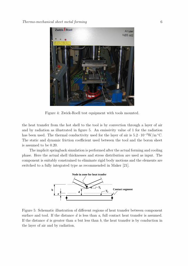
Thermo-mechanical sheet metal forming 6
Figure 4: Zwick-Roell test equipment with tools mounted.
the heat transfer from the hot shell to the tool is by convection through a layer of air
and by radiation as illustrated in figure 5. An emissivity value of 1 for the radiation
has been used. The thermal conductivity used for the layer of air is 5.2 · 10−2W/m ◦C.
The static and dynamic friction coefficient used between the tool and the boron sheet
is assumed to be 0.20.
The implicit springback simulation is performed after the actual forming and cooling
phase. Here the actual shell thicknesses and stress distribution are used as input. The
component is suitably constrained to eliminate rigid body motions and the elements are
switched to a fully integrated type as recommended in Maker [21].
da
b Contact segmentT1
T2
Node in zone for heat tranfer
Figure 5: Schematic illustration of different regions of heat transfer between component
surface and tool. If the distance d is less than a, full contact heat transfer is assumed.
If the distance d is greater than a but less than b, the heat transfer is by conduction in
the layer of air and by radiation.
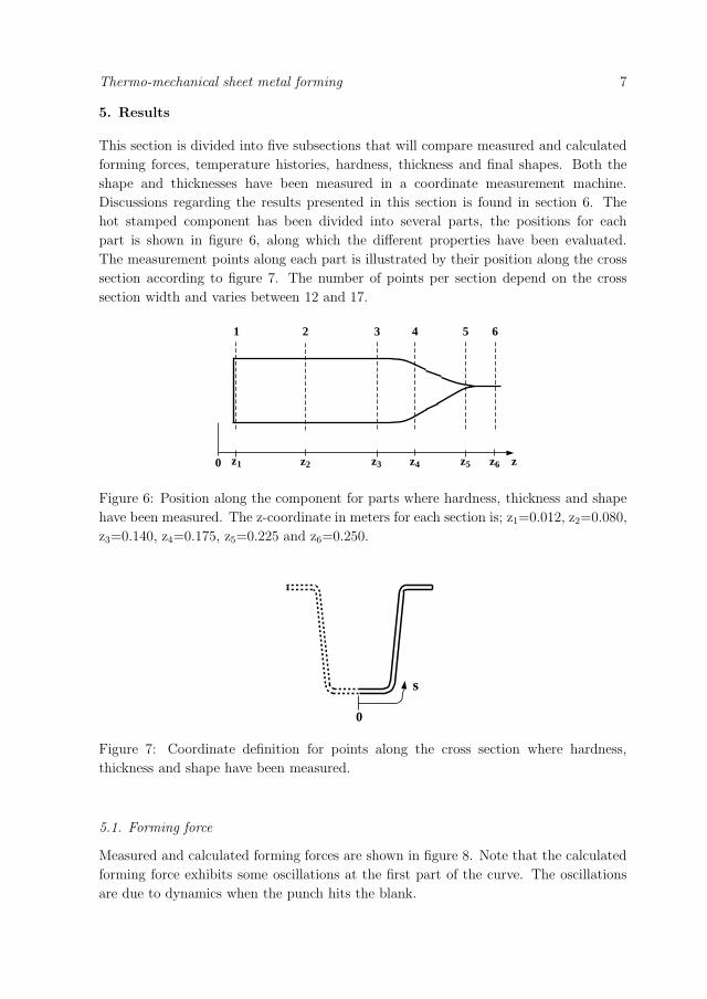
Thermo-mechanical sheet metal forming 7
5. Results
This section is divided into five subsections that will compare measured and calculated
forming forces, temperature histories, hardness, thickness and final shapes. Both the
shape and thicknesses have been measured in a coordinate measurement machine.
Discussions regarding the results presented in this section is found in section 6. The
hot stamped component has been divided into several parts, the positions for each
part is shown in figure 6, along which the different properties have been evaluated.
The measurement points along each part is illustrated by their position along the cross
section according to figure 7. The number of points per section depend on the cross
section width and varies between 12 and 17.
z
1 2 3 4 5 6
z1 z2 z3 z4 z5 z60
Figure 6: Position along the component for parts where hardness, thickness and shape
have been measured. The z-coordinate in meters for each section is; z1=0.012, z2=0.080,
z3=0.140, z4=0.175, z5=0.225 and z6=0.250.
s
0
Figure 7: Coordinate definition for points along the cross section where hardness,
thickness and shape have been measured.
5.1. Forming force
Measured and calculated forming forces are shown in figure 8. Note that the calculated
forming force exhibits some oscillations at the first part of the curve. The oscillations
are due to dynamics when the punch hits the blank.
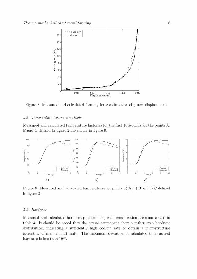
Thermo-mechanical sheet metal forming 8
0 0.01 0.02 0.03 0.04 0.050
20
40
60
80
100
120
140
160
Displacement (m)
Form
ing
forc
e (k
N)
CalculatedMeasured
Figure 8: Measured and calculated forming force as function of punch displacement.
5.2. Temperature histories in tools
Measured and calculated temperature histories for the first 10 seconds for the points A,
B and C defined in figure 2 are shown in figure 9.
0 2 4 6 8 100
20
40
60
80
100
Time (s)
Tem
pera
ture
(°C
)
CalculatedMeasured
a)
0 2 4 6 8 100
20
40
60
80
100
120
140
Time (s)
Tem
pera
ture
(°C
)
CalculatedMeasured
b)
0 2 4 6 8 100
20
40
60
80
100
Time (s)
Tem
pera
ture
(°C
)
CalculatedMeasured
c)
Figure 9: Measured and calculated temperatures for points a) A, b) B and c) C defined
in figure 2.
5.3. Hardness
Measured and calculated hardness profiles along each cross section are summarized in
table 3. It should be noted that the actual component show a rather even hardness
distribution, indicating a sufficiently high cooling rate to obtain a microstructure
consisting of mainly martensite. The maximum deviation in calculated to measured
hardness is less than 10%.
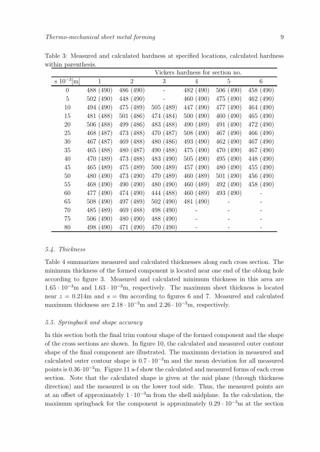
Thermo-mechanical sheet metal forming 9
Table 3: Measured and calculated hardness at specified locations, calculated hardness
within parenthesis.Vickers hardness for section no.
s 10−3[m] 1 2 3 4 5 6
0 488 (490) 486 (490) - 482 (490) 506 (490) 458 (490)
5 502 (490) 448 (490) - 460 (490) 475 (490) 462 (490)
10 494 (490) 475 (489) 505 (489) 447 (490) 477 (490) 464 (490)
15 481 (488) 501 (486) 474 (484) 500 (490) 460 (490) 465 (490)
20 506 (488) 499 (486) 483 (488) 490 (489) 491 (490) 472 (490)
25 468 (487) 473 (488) 470 (487) 508 (490) 467 (490) 466 (490)
30 467 (487) 469 (488) 480 (486) 493 (490) 462 (490) 467 (490)
35 465 (488) 480 (487) 490 (488) 475 (490) 470 (490) 467 (490)
40 470 (489) 473 (488) 483 (490) 505 (490) 495 (490) 448 (490)
45 465 (489) 475 (489) 500 (489) 457 (490) 480 (490) 455 (490)
50 480 (490) 473 (490) 470 (489) 460 (489) 501 (490) 456 (490)
55 468 (490) 490 (490) 480 (490) 460 (489) 492 (490) 458 (490)
60 477 (490) 474 (490) 444 (488) 460 (489) 493 (490) -
65 508 (490) 497 (489) 502 (490) 481 (490) - -
70 485 (489) 469 (488) 498 (490) - - -
75 506 (490) 480 (490) 488 (490) - - -
80 498 (490) 471 (490) 470 (490) - - -
5.4. Thickness
Table 4 summarizes measured and calculated thicknesses along each cross section. The
minimum thickness of the formed component is located near one end of the oblong hole
according to figure 3. Measured and calculated minimum thickness in this area are
1.65 · 10−3m and 1.63 · 10−3m, respectively. The maximum sheet thickness is located
near z = 0.214m and s = 0m according to figures 6 and 7. Measured and calculated
maximum thickness are 2.18 · 10−3m and 2.26 · 10−3m, respectively.
5.5. Springback and shape accuracy
In this section both the final trim contour shape of the formed component and the shape
of the cross sections are shown. In figure 10, the calculated and measured outer contour
shape of the final component are illustrated. The maximum deviation in measured and
calculated outer contour shape is 0.7 · 10−3m and the mean deviation for all measured
points is 0.36·10−3m. Figure 11 a-f show the calculated and measured forms of each cross
section. Note that the calculated shape is given at the mid plane (through thickness
direction) and the measured is on the lower tool side. Thus, the measured points are
at an offset of approximately 1 · 10−3m from the shell midplane. In the calculation, the
maximum springback for the component is approximately 0.29 · 10−3m at the section

Thermo-mechanical sheet metal forming 10
Table 4: Measured and calculated thickness at specified locations, calculated thickness
within parenthesis.
Thickness 10−3[m] for section no.
s 10−3[m] 1 2 3 4 5 6
0 2.04 (1.99) 1.96 (1.96) - 1.92 (1.93) 2.10 (2.10) 1.98 (1.95)
5 1.99 (1.99) 1.96 (1.96) - 1.90 (1.94) 2.07 (2.05) 1.99 (1.95)
10 2.00 (1.99) 1.95 (1.96) 1.97 (1.97) 1.91 (1.99) 2.07 (2.03) 1.98 (1.96)
15 2.04 (2.04) 1.93 (1.97) 2.00 (1.96) 1.87 (1.91) 2.08 (2.02) 2.01 (1.96)
20 1.97 (2.01) 1.91 (1.97) 1.92 (1.94) 1.83 (1.93) 2.09 (2.02) 2.00 (1.97)
25 1.96 (1.99) 1.93 (1.94) 1.89 (1.93) 1.93 (1.99) 2.07 (2.00) 1.99 (1.97)
30 1.96 (1.99) 1.94 (1.95) 1.92 (1.91) 1.98 (2.01) 2.03 (2.02) 1.98 (1.97)
35 1.96 (1.99) 1.94 (1.97) 1.92 (1.94) 1.99 (2.01) 2.03 (2.01) 2.00 (1.97)
40 1.96 (1.99) 1.94 (1.97) 1.93 (1.94) 1.99 (2.03) 2.09 (2.02) 2.00 (1.97)
45 1.98 (1.99) 1.94 (1.97) 1.92 (1.94) 1.99 (2.04) 2.03 (1.99) 2.00 (1.98)
50 1.98 (1.99) 1.93 (1.97) 1.86 (1.93) 1.97 (2.01) 2.02 (1.98) 2.01 (1.98)
55 1.97 (1.99) 1.91 (1.97) 1.84 (1.92) 2.00 (2.00) 1.98 (1.98) 1.98 (1.98)
60 2.00 (1.99) 1.99 (1.95) 1.93 (1.88) 1.98 (1.99) 1.95 (1.98) -
65 2.01 (1.99) 1.99 (1.99) 2.00 (1.95) 2.00 (1.98) - -
70 1.97 (2.00) 1.99 (1.99) 2.02 (1.93) - - -
75 1.97 (1.99) 1.99 (1.99) 2.08 (2.02) - - -
80 1.97 (1.99) 1.99 (1.99) 2.06 (2.05) - - -
for z = 0.012m according to figure 6.
Figure 10: Calculated trim contour of the final component is given as lines, and a cross
indicates a measured point. Note that only one half of the actual geometry is shown.
6. Discussion
The overall correspondence between measured and calculated forming forces is quite
satisfactory, indicating that the stress-strain data used are adequate. Note that the
mechanical response during the forming phase is mainly governed by the austenite.
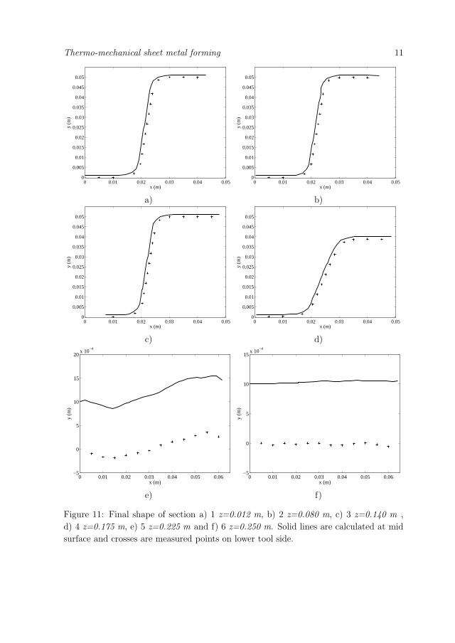
Thermo-mechanical sheet metal forming 11
0 0.01 0.02 0.03 0.04 0.050
0.005
0.01
0.015
0.02
0.025
0.03
0.035
0.04
0.045
0.05
x (m)
y (m
)
a)
0 0.01 0.02 0.03 0.04 0.050
0.005
0.01
0.015
0.02
0.025
0.03
0.035
0.04
0.045
0.05
x (m)
y (m
)
b)
0 0.01 0.02 0.03 0.04 0.050
0.005
0.01
0.015
0.02
0.025
0.03
0.035
0.04
0.045
0.05
x (m)
y (m
)
c)
0 0.01 0.02 0.03 0.04 0.050
0.005
0.01
0.015
0.02
0.025
0.03
0.035
0.04
0.045
0.05
x (m)
y (m
)
d)
0 0.01 0.02 0.03 0.04 0.05 0.06−5
0
5
10
15
20x 10
−4
x (m)
y (m
)
e)
0 0.01 0.02 0.03 0.04 0.05 0.06−5
0
5
10
15x 10
−4
x (m)
y (m
)
f)
Figure 11: Final shape of section a) 1 z=0.012 m, b) 2 z=0.080 m, c) 3 z=0.140 m ,
d) 4 z=0.175 m, e) 5 z=0.225 m and f) 6 z=0.250 m. Solid lines are calculated at mid
surface and crosses are measured points on lower tool side.

Thermo-mechanical sheet metal forming 12
The calculated component shows small amounts of ferrite (<3%) at the upper and
lower radius. This is a consequence of the straining of the material in the austenitic state
which accelerates the nucleation and growth of ferrite. The maximum volume fraction
bainite (∼1.2%) is found close to the oblong hole where the sheet thickness is reduced.
The remainder of the microstructure consists mainly of martensite because pearlite is
present in negligible amounts, less than 0.3%.
The temperature measurements in the tools using the insert type of thermoele-
ments, give a rather large variation in measured temperature as has been observed in
previous experiments. The variation can be as high as 10 ◦C at the peak of the tem-
perature transient. This is due to the difficulties to ensure good thermal contact of the
thermoelement tip in the drilled hole even if heat conducting paste has been applied.
Deviations in tool temperatures may also be a consequence from the simulation due to
the prescribed displacement of the upper tool until nominal sheet thickness is reached.
This may also affect the final material state and hardness distribution since a more
evenly distributed contact situation is reached between the tool and the blank com-
pared to a situation where a prescribed force is used in the simulation. The calculated
and measured temperature histories deviate less than 13 ◦C within the time interval
considered, which can be regarded acceptable.
Comparing measured and calculated thicknesses indicates small deviations, and
consequently an adequate strain distribution within the component is obtained.
The predicted component shape is in good agreement with the measured, indicating
that the implemented models can be used as predictive tools in the product development
phase. Therefore, expensive tool prototypes can be avoided and accurate adjustments
of the blank trim shape can be made.
Cold forming of a similar component in a ultra high strength steel quality, would
cause reduced formability and generate excessive springback.
7. Conclusions
In the present work, a numerical FE-simulation of a thermo-mechanical forming of a
high strength component has been compared to the corresponding experiment. The
comparisons include forming force, thickness-, hardness distribution and predictions of
the final component shape. All comparisons show acceptable agreement. It is concluded
that the used methods provide an effective tool for design work during the product
development phase.
The implemented models for predicting both the phase evolution as well as the
mechanical material model can also be used in predicting designed soft zones, e.g. trigger
zones for controlled collapse of safety components.

Thermo-mechanical sheet metal forming 13
8. Acknowledgments
The financial support from Gestamp HardTech AB and the Research Council of
Norrbotten are gratefully acknowledged.
REFERENCES 14
References
[1] G. Bergman and M. Oldenburg. A finite element model for thermomechanical
analysis of sheet metal forming. Int. J. Numer. Meth. Engng., 59:1167–1186, 2004.
[2] J. Wu, L. Zhang, J. Chen, and W. Wang. Simulation of hot stamping process
with advanced material modeling. In Innovations in steel sheet and bar products
and processing, and modeling and testing of steel structures, number 0168. SAE
International, 2004.
[3] J.S. Kirkaldy and D. Venugopalan. Prediction of microstructure and hardenability
in low alloy steels. In A.R. Marder and J.I. Goldstein, editors, Int. conference on
phase transformations in ferrous alloys, pages 125–148, Philadelphia, Oct. 1983.
[4] M.V. Li, D.V. Niebuhr, L.L. Meekisho, and D.G. Atteridge. A computational model
for the prediction of steel hardenability. Metallurgical and Materials Transactions,
29B(3):661–672, June 1998.
[5] D. Watt, L. Coon, M. Bibby, J. Goldak, and C. Henwood. An algorithm for
modelling microstructural development in weld heat-affected zones (part a) reaction
kinetics. Acta Metallurgica, 36(11):3029–3035, 1988.
[6] J.B. Leblond, G. Mottet, and J.C. Devaux. A theoretical and numerical approach to
the plastic behaviour of steels during phase transformations-i. derivation of general
relations. J. Mech. Phys. Solids, 34(4):395–409, 1986.
[7] J.B. Leblond, G. Mottet, and J.C. Devaux. A theoretical and numerical approach
to the plastic behaviour of steels during phase transformations-ii. study of classical
plasticity for ideal-plastic phases. J. Mech. Phys. Solids, 34(4):411–432, 1986.
[8] J.B. Leblond, J. Devaux, and J.C. Devaux. Mathematical modelling of
transformation plasticity in steels i: Case of ideal-plastic phases. International
Journal of Plasticity, 5:551–572, 1989.
[9] J.B. Leblond. Mathematical modelling of transformation plasticity in steels ii:
Coupling with strain hardening phenomena. International Journal of Plasticity, 5:
573–591, 1989.
[10] P. Akerstrom, G. Bergman, and M. Oldenburg. Numerical implementation of a
constitutive model for simulation of hot stamping. Submitted for publication.
[11] Orvar Supreme. Uddeholm Tooling Svenska AB, Box 148, SE-631 03 Eskilstuna,
Sweden, 3 edition, April 2003.
[12] G. Bergman. Modelling and simulation of simultaneous forming and quenching.
PhD thesis, Lulea University of Technology, 1999.
[13] P. Akerstrom, B. Wikman, and M. Oldenburg. Material parameter estimation for
boron steel from simultaneous cooling and compression experiments. Modelling
Simul. Mater. Sci. Eng., 13:1291–1308, 2005.
[14] S. Sjostrom. The calculation of quench stresses in steel. PhD thesis, Linkoping
University, Linkoping Sweden, 1982.
REFERENCES 15
[15] Rudiono and Y. Tomota. Application of the secant method to prediction of flow
curves in multi-microstructure steels. Acta. mater., 45(5):1923–1929, 1997.
[16] C. Huang, E.B. Hawbolt, X. Chen, T.R. Meadowcroft, and D.K. Matlock. Flow
stress modeling and warm rolling simulation behavior of two ti-nb interstitial-free
steels in the ferrite region. Acta mater., 49:1445–1452, 2001.
[17] R. Nakkalil, J.R. Hornaday Jr., and M. Nabil Bassim. Characterization of the
compression properties of rail steels at high temperatures and strain rates. Materials
Science and Engineering, A141:247–260, 1991.
[18] S. Petit-Grostabussiat, L. Taleb, and J-F. Jullien. Experimental results on classical
plasticity of steels subjected to structural transformations. International Journal
of Plasticity, 20:1371–1386, 2004.
[19] M. Eriksson, M. Oldenburg, M.C. Somani, and L.P. Karjalainen. Testing and
evaluation of material data for analysis of forming and hardening of boron steel
components. Modelling Simul. Mater. Sci. Eng., 10:1–18, 2002.
[20] M.C. Somani, L.P. Karjalainen, M. Eriksson, and M. Oldenburg. Dimensional
changes and microstructural evolution in a b-bearing steel in the simulated forming
and quenching process. ISIJ International, 41(4):361–367, 2001.
[21] B.N. Maker. Implicit analysis with ls-dyna. LSTC, Feb 2001.