Linköpings universitet

Institutionen för ekonomisk och industriell utveckling

Examensarbete 2015| LIU-IEI-TEK-A—20/03906--SE

MASTER THESIS

Modelling and Simulation of Fan Performance using CFD

Group

Shreyasu Subramanya (shrsu040)

Linköpings universitet

SE-581 83 Linköping, Sweden

013-28 10 00, www.liu.se

Linköpings universitet

Institutionen för ekonomisk och industriell utveckling

Avdelning

Examensarbete 2015| LIU-IEI-TEK-A—20/03906--SE

Modelling and Simulation of Fan Performance using CFD

Group

Shreyasu Subramanya (shrsu040)

Academic supervisor: Johan Renner

Industrial supervisor: Bingbing Shi

Industrial Manager: Christian Nyberg

Examiner: Roland Gårdhagen

i

Abstract

Performance of vacuum cleaners are greatly affected by factors such as static pressure, airflow

rate and efficiency. In this thesis work, attempt has been made to design a fan to meet the

requirements of suction static pressure and air flow rate and in the process understand the fan

design parameters that affect these performance parameters. Parametric study has been

conducted for the same, by choosing six fan design parameters. Additionally, ways to increase

the fan efficiency has been investigated during the parametric study.

Computational Fluid Dynamics is used to visualize the flow inside the fan casing and further

to simulate fan performance at an operational point. Steady state RANS and moving reference

frames was used to model the turbulence in the fluid flow and rotation of the fan, respectively.

Performance curve showing the relation between static suction pressure and mass flow rate is

plotted for the base model is in proximity to the required performance. Parametric study was

conducted on the six fan design parameters: Fan diameter, number of impeller blades, blade

outlet angle, radius of the curve connecting inlet to outlet section of the fan, diffuser exit length

and splitter blade length. The range for each parameter analysis was restricted so that static

pressure values are around the required performance.

Large performance variation was found with design parameters: fan diameter, blade outlet

angle, radius of the curve connecting inlet to outlet section of the fan and diffuser exit length.

This variation at low mass flow rate can be majorly attributed to the randomness in the flow

captured by entropy contours. At high mass flow rate, blockage in the flow visualized by

pressure contours reasoned for the performance variation. No significant performance

variation was observed when design parameters such as number of blades and splitter blade

length were varied. Larger variation of these parameters is required to see better variation.

ii

Acknowledgements

First and foremost, I would like to express my gratitude to my examiner at Linkoping

University, Roland Gårdhagen, for his guidance and constant support throughout my work,

right from providing technical support and required tools to assisting and examining my work.

My sincere thanks to my supervisor at the university, Johan Renner for his constant inputs and

feedbacks that helped me improve my work.

It was truly a great experience to carry out this thesis work at Husqvarna Group under the ‘Dust

and Slurry R&D’ team. I am grateful to my manager Christian Nyberg for all the support and

guidance. Thank you for also providing me with all the facilities in the office that helped

immensely in carrying out this work. I would also like to thank my supervisor at the company,

Bingbing Shi, for encouraging throughout this work. Constant inputs and suggestions provided

by you helped me overcoming the technical challenges during this work. My extended thanks

to the entire Dust and Slurry R&D team, everyone has been a great help. I also like to thank

other team members at Husqvarna for providing me the resources and sharing their subject

expertise.

I vow my thanks to my family members who have always been my support system. My regards

to my friends for sharing ideas that helped me to document this work in a right way. I cannot

express my complete gratitude for my family and friends by mere words here. Their support is

beyond it for which I will be ever grateful.

It is worth mentioning that this thesis work was carried out when the world was challenged

with global pandemic, COVID-19. The encouragement and motivation from these people have

helped me to complete my work on time. I would like to mention that I am solely responsible

for any discrepancies found in this work.

iii

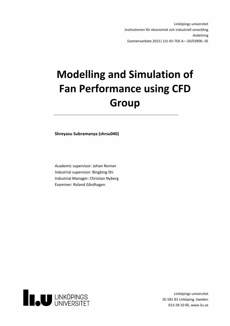
Nomenclature

Latin

Symbol Description Unit

T Temperature K

U Velocity magnitude m s-1

f Frequency Hz

Q

D

Ds

N

Ns

R

P

∆𝑃

L

t

ui

xi

h

∆Vi

r

GCI21 fine

e21a

e21ext

Mass flow rate

Diameter

Specific Diameter

Rotation Speed

Specific Speed

Radius

Pressure

Pressure difference

Length

Time

Velocity vector component

Position vector component

Representative cell size

Volume of ith cell

Grid refinement factor

Fine-grid convergence index

Approximate relative error

Extrapolated relative error

m3 s-1

m

-

RPM

-

m

Pa

Pa

m

s

m s-1

m

m3

m3

-

-

-

-

Greek

Symbol Description Unit

𝜌

µ

ε

Density

Dynamics viscosity

Eddy viscosity

Kg m-3

kg m-1 s-1

N s m-2

𝛱𝑖𝑗

φ

ϴ

Pressure-velocity gradient tensor

Flow Coefficient

Theta

m2 s-3

-

Deg

iv

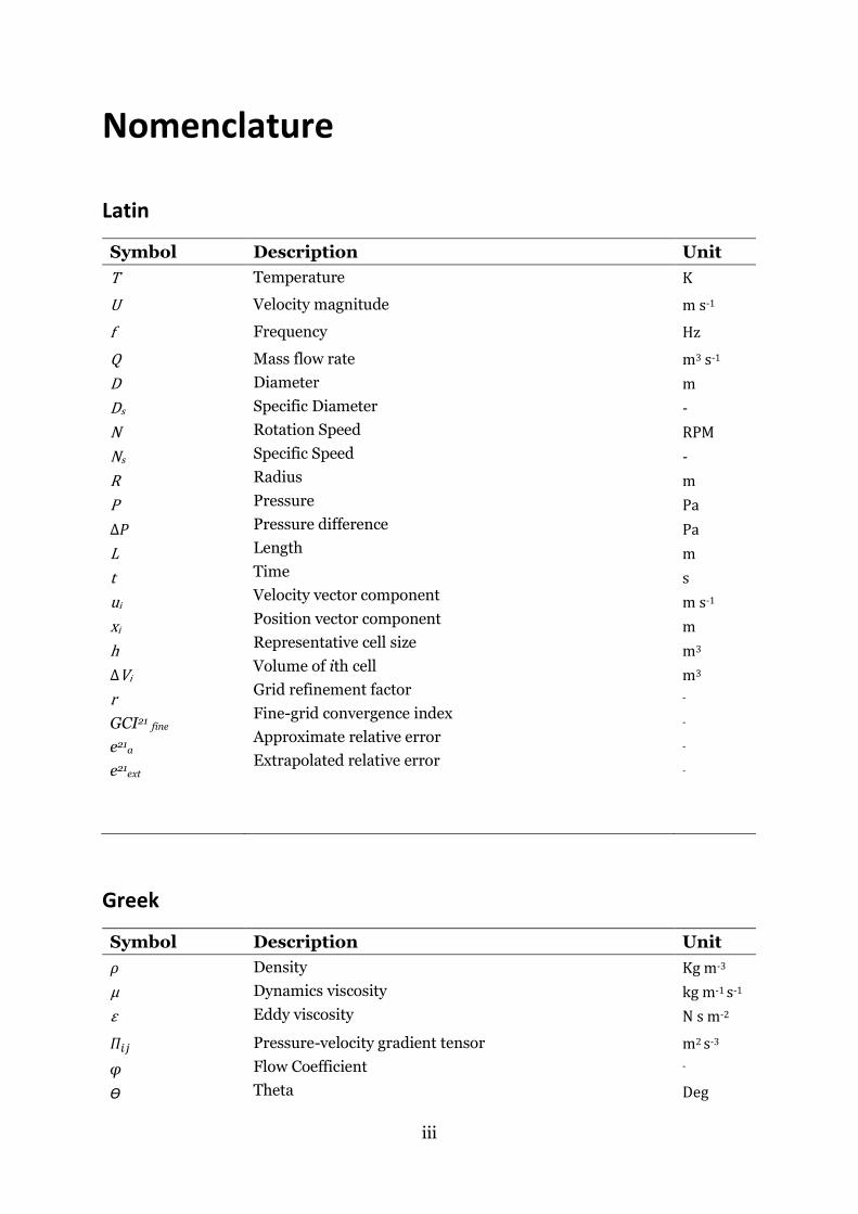
Symbol

β

τi,j

Ѡ

φk

η

ν

Description

Outlet blade angle

Stress components

Angular velocity

Solution on the kth grid

Characteristic length

Characteristic velocity

Unit

Deg

N m-2

Rad s-1

-

m

m s-1

Abbreviations and Acronyms

Letter Description

CFD Computational fluid dynamics

HEPA

TKE

RANS

RE

High-Efficiency Particulate Air

Turbulent Kinetic Energy

Reynolds Averaged Navier-Stokes

Richardson Extrapolation

v

Contents Abstract ............................................................................................................................. i

Acknowledgements .......................................................................................................... ii

Nomenclature .................................................................................................................. iii

Contents ........................................................................................................................... v

1. Introduction .................................................................................................................. 1

1.1 Background ............................................................................................................................. 1

1.2 Literature Survey .................................................................................................................... 3

1.3 Aim .......................................................................................................................................... 4

1.3.1 Research questions ....................................................................................................................... 4

1.4 Resources and Limitations ...................................................................................................... 5

2. Theory .......................................................................................................................... 6

2.1 Turbomachines ....................................................................................................................... 6

2.1.1 Centrifugal Compressor and components .................................................................................... 6

2.2 Cordier Diagram ...................................................................................................................... 8

2.3 Fan performance curves ......................................................................................................... 9

2.4 Computational Fluid Dynamics ............................................................................................ 10

2.4.1 Governing equations ................................................................................................................... 11

2.4.2 Turbulence and Turbulence modelling ....................................................................................... 11

2.4.3 Wall region .................................................................................................................................. 12

2.4.4 SST k-Omega Turbulence Model ................................................................................................. 13

2.4.5 Limitations with turbulence modelling ....................................................................................... 14

3. Method ....................................................................................................................... 15

3.1 Fan Design ............................................................................................................................. 15

3.2 Geometry .............................................................................................................................. 16

3.3 Parameteric Design ............................................................................................................... 18

3.4 Meshing ................................................................................................................................. 19

3.4.1 Mesh sensitive study................................................................................................................... 20

3.5 Physics ................................................................................................................................... 22

3.6 Boundary conditions ............................................................................................................. 22

3.7 Convergence.......................................................................................................................... 23

3.8 Impeller Rotation .................................................................................................................. 23

3.8.1 Moving reference frame ............................................................................................................. 23

3.8.2 Interfaces .................................................................................................................................... 23

4. Results ........................................................................................................................ 25

4.1 Base Geometry ...................................................................................................................... 25

4.1.1 Performance Curve ..................................................................................................................... 25

vi

4.1.2 Flow Through Base Geometry..................................................................................................... 26

4.2 Parametric study ................................................................................................................... 30

4.2.1 Fan Diameter .............................................................................................................................. 30

4.2.2 Outlet Blade Angle ...................................................................................................................... 32

4.2.3 Number of Impeller Blades ......................................................................................................... 36

4.2.4 Curvature Radius ......................................................................................................................... 38

4.2.5 Diffuser Exit Length ..................................................................................................................... 40

4.2.6 Splitter Blade Length ................................................................................................................... 42

5. Discussion ................................................................................................................... 43

5.1 Computational Domain, Geometry and Mesh..................................................................... 43

5.3 Choice of Turbulence Model and Physics Used in Simulations ........................................... 43

5.3 Base Model ........................................................................................................................... 44

5.4 Parametric Study .................................................................................................................. 45

5.4.1 Fan Diameter .............................................................................................................................. 45

5.4.2 Outlet Blade angle ...................................................................................................................... 45

5.4.3 Number of impeller blades ......................................................................................................... 46

5.4.4 Curvature Radius ......................................................................................................................... 46

5.4.5 Diffuser exit length ..................................................................................................................... 47

5.4.6 Length of Splitter Blade .............................................................................................................. 47

6. Conclusions ................................................................................................................. 48

References ...................................................................................................................... 49

1

1. Introduction

Vacuum cleaners, in general, is used to draw dust particles in the surroundings. In industries,

it is of higher significance as the end product of any industry yields ultrafine dust particles that

may be toxic to the workers and environment, so industrial vacuum cleaners are used as filters.

Today, many industrial vacuum cleaners are delivered to the market, but the size and

performance of the vacuum cleaners are very often debated. Users are always looking for high

performance and small-size product. Minimizing the size of vacuum cleaners and improving

performance indicates scaling-down main components such as motor and fan. This promotes

the manufacturers to trade-off between the size and performance of the machine.

In this master thesis, the central focus has been on one of the main components of vacuum

cleaner, that is the ‘fan’. Designing of new component requires the knowledge on the

component and how the design changes to the component impacts the output performance.

Hence in this thesis work, an attempt is made to gain knowledge on impact of the fan design

parameters on fan static pressure and air flow rate. Few design parameters are analyzed during

this work to understand how these parameters affect the performance. Work further deals with

understanding the influence of fan construction and blade design on fan size. This thesis work

is carried out with the knowledge in working and designing of compressor fan, CAD

(Computer-aided design) modelling software and Computational Fluid Dynamics (CFD).

1.1 Background

Industrial vacuum cleaners play a salient role at the construction sites where operations such

as cutting, drilling, and grinding of concrete, brick and other hard materials are customary. As

an outcome of these activities, dust particles are suspended into the surroundings and spread

wider into the environment. Microscopic, respirable dust particles that are toxic can be inhaled

by humans (especially construction workers) and other living organisms that lead to serious

and sometimes life-threating health conditions. On the other hand, dust particles can cause

wear and tear of equipment in the working area [1]. To avoid these consequences, dust-

collection devices such as vacuum cleaners must be implemented at the source along with

construction workers wearing personal protective equipment such as air-purifying respirators.

The basic mechanism of vacuum cleaners, be it for household or industrial purpose remains

the same. The negative pressure inside the vacuum cleaner creates a suction to suck the

ambient air into it. The dirt-rich air, inside the vacuum cleaner is passed through the dust bag

that acts as air filter. This bag is impermeable to dust particles, purifies the air and lets it out.

Basic working of vacuum cleaner can be visualized from Figure 1. The equipment involved in

this thesis work consists of two dust bags, cyclone tank to remove heavier particles and mainly

HEPA (High-Efficiency Particulate Air) filters for ultrafine air purification. Fan is the heart of

vacuum machines as it generates negative pressure inside the equipment.

2

Figure 1 : Basic working of vacuum cleaner. Source: Google images

Therefore, it is essential to develop efficient fan and enlarge stable operating range of this

machine. Factors such as efficiency, operating in stable range, affect the power and

maintenance of the machine along with the rate at which the dust is collected. To obtain a high

efficiency vacuum device, the vacuum fan should be able to generate high suction power with

minimum possible energy consumption.

Understanding the factors affecting the fan design and the air flow inside it is the starting point

in the fan development process. Physical prototyping of various fan designs and testing its

performance helps in analyzing the flow dynamics. However, this is not a preferred way of

study as it involves iterative process of developing a new fan design and testing its performance

which can be tedious, time- consuming and expensive.

With the computational power available today, computational fluid dynamics (CFD) can be

used for fan development and analysis. CFD is a numerical tool where governing equations of

the flow are solved in the simulation [2]. The inertial and viscous forces of the fluid systems

are modelled to understand the flow physics and for the visualization purpose. Various

turbulence models are available to represent turbulent flow in CFD but selecting a particular

model depends on aspects such as flow phenomenon and trade-off between computational

time and accuracy of result. The analysis of flow in CFD is classified into two states on the basis

of taking time into account, the state which considers the time factor is known as unsteady

state and the state in which time factor is insignificant is known as steady state. The density

variations in the fluid is negligible for flow with Mach number less than 0.3 and can be

considered as incompressible fluid. Density variations is of higher significance for the flow

greater than Mach 0.3 until Mach 0.8 and compressibility needs to be considered. Flow is said

to be in transonic region above Mach 0.8 until Mach 1.2 where shock waves appear. Flow can

be either viscous or inviscid. In viscous flows, shear forces between the fluid layers is dominant

and significant.

The ability to simulate airflow through the fan in the CFD software helps in better

understanding of the flow physics inside the fan. This enables effective modelling of flow

resistance inside the fan housing and turbulence of airflow thus allowing modifications to the

fan geometry to achieve high efficiency and performance requisite. Hence, the capabilities of

CFD and CAD are utilized in the best way for this application.

It is important for the fan to work within a certain operating range in order to have an extended

life and high efficiency. CFD helps in determining the operating range and limitations without

having to damage the test components, which is otherwise evident in physical tests. Operating

3

the fan outside a certain range causes surge and choke that results in physical damage of the

fan.

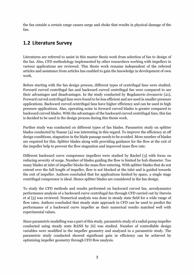
1.2 Literature Survey

Literatures are referred to assist in this master thesis work from selection of fan to design of

the fan. Also, CFD methodology implemented by other researchers working with impellers in

various applications are reviewed. This thesis work remains independent of the referred

articles and assistance from articles has enabled to gain the knowledge in development of own

work.

Before starting with the fan design process, different types of centrifugal fans were studied.

Forward curved centrifugal fan and backward curved centrifugal fan were compared to see

their advantages and disadvantages. In the study conducted by Bogdanovic-Jovanovic [21],

Forward curved centrifugal fans were found to be less efficient and are used in smaller pressure

applications. Backward curved centrifugal fans have higher efficiency and can be used in high

pressure applications. Also, operating noise in forward curved blades is greater compared to

backward curved blades. With the advantages of the backward curved centrifugal fans, this fan

is decided to be used in the design process during this thesis work.

Further study was conducted on different types of fan blades. Parametric study on splitter

blades conducted by Nassar [4] was interesting in this regard. To improve the efficiency at off

design conditions, stagnation in the blade passage needs to be avoided. More number of blades

are required for this. Splitter blades along with providing guidance for the flow at the exit of

the impeller help to prevent the flow stagnation and improved mass flow rate.

Different backward curve compressor impellers were studied by Rachel [3] with focus on

reducing severity of surge. Number of blades guiding the flow is limited by hub diameter. Too

many blades at inlet of impeller blocks the mass flow entering. With splitter blades that do not

extend over the full length of impeller, flow is not blocked at the inlet and is guided towards

the exit of impeller. Authors concluded that for applications limited by space, a single stage

centrifugal compressor is ideal. Hence splitter blades are considered in the fan design.

To study the CFD methods and results performed on backward curved fan, aerodynamics

performance analysis of a backward curve centrifugal fan through CFD carried out by Darwin

et al [5] was reviewed. Numerical analysis was done in steady state field for a wide range of

flow rates. Authors concluded that steady state approach in CFD can be used to predict the

performance of a backward curve impeller as their numerical results matched well with

experimental values.

Since parametric modelling was a part of this study, parametric study of a radial pump impeller

conducted using steady state RANS by [6] was studied. Number of controllable design

variables were modified in the impeller geometry and analyzed in a parametric study. The

parametric study conducted showed significant gain in efficiency can be achieved by

optimizing impeller geometry through CFD flow analysis.

4

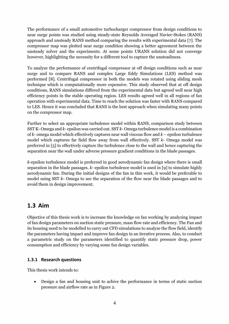
The performance of a small automotive turbocharger compressor from design conditions to

near surge points was studied using steady-state Reynolds Averaged Navier-Stokes (RANS)

approach and unsteady RANS method comparing the results with experimental data [7]. The

compressor map was plotted near surge condition showing a better agreement between the

unsteady solver and the experiments. At some points URANS solution did not converge

however, highlighting the necessity for a different tool to capture the unsteadiness.

To analyze the performance of centrifugal compressor at off design conditions such as near

surge and to compare RANS and complex Large Eddy Simulations (LES) method was

performed [8]. Centrifugal compressor in both the models was rotated using sliding mesh

technique which is computationally more expensive. This study observed that at off design

conditions, RANS simulations differed from the experimental data but agreed well near high

efficiency points in the stable operating region. LES results agreed well in all regions of fan

operation with experimental data. Time to reach the solution was faster with RANS compared

to LES. Hence it was concluded that RANS is the best approach when simulating many points

on the compressor map.

Further to select an appropriate turbulence model within RANS, comparison study between

SST K- Omega and k- epsilon was carried out. SST k- Omega turbulence model is a combination

of k- omega model which effectively captures near wall viscous flow and k – epsilon turbulence

model which captures far field flow away from wall effectively. SST k- Omega model was

preferred in [5] to effectively capture the turbulence close to the wall and hence capturing the

separation near the wall under adverse pressure gradient conditions in the blade passages.

k-epsilon turbulence model is preferred in good aerodynamic fan design where there is small

separation in the blade passages. k- epsilon turbulence model is used in [9] to simulate highly

aerodynamic fan. During the initial designs of the fan in this work, it would be preferable to

model using SST k- Omega to see the separation of the flow near the blade passages and to

avoid them in design improvement.

1.3 Aim

Objective of this thesis work is to increase the knowledge on fan working by analyzing impact

of fan design parameters on suction static pressure, mass flow rate and efficiency. The Fan and

its housing need to be modelled to carry out CFD simulations to analyze the flow field, identify

the parameters having impact and improve fan design in an iterative process. Also, to conduct

a parametric study on the parameters identified to quantify static pressure drop, power

consumption and efficiency by varying some fan design variables.

1.3.1 Research questions

This thesis work intends to:

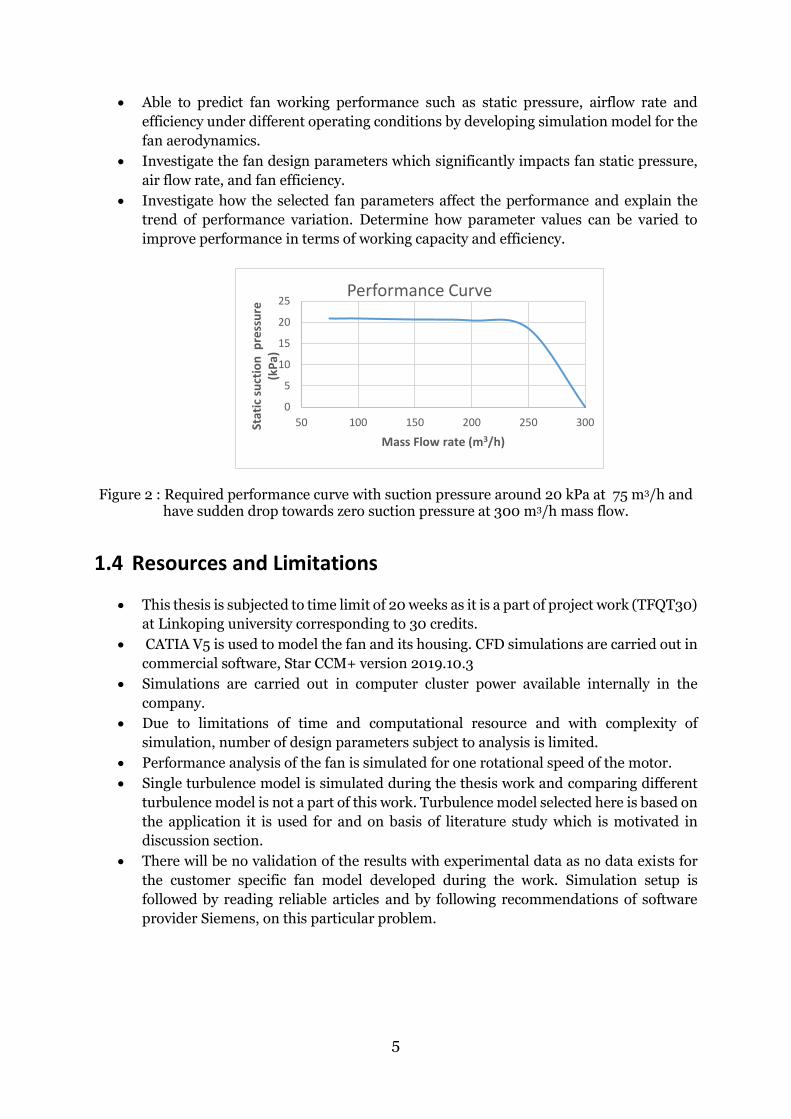
• Design a fan and housing unit to achive the performance in terms of static suction

pressure and airflow rate as in Figure 2.

5

• Able to predict fan working performance such as static pressure, airflow rate and

efficiency under different operating conditions by developing simulation model for the

fan aerodynamics.

• Investigate the fan design parameters which significantly impacts fan static pressure,

air flow rate, and fan efficiency.

• Investigate how the selected fan parameters affect the performance and explain the

trend of performance variation. Determine how parameter values can be varied to

improve performance in terms of working capacity and efficiency.

Figure 2 : Required performance curve with suction pressure around 20 kPa at 75 m3/h and have sudden drop towards zero suction pressure at 300 m3/h mass flow.

1.4 Resources and Limitations

• This thesis is subjected to time limit of 20 weeks as it is a part of project work (TFQT30)

at Linkoping university corresponding to 30 credits.

• CATIA V5 is used to model the fan and its housing. CFD simulations are carried out in

commercial software, Star CCM+ version 2019.10.3

• Simulations are carried out in computer cluster power available internally in the

company.

• Due to limitations of time and computational resource and with complexity of

simulation, number of design parameters subject to analysis is limited.

• Performance analysis of the fan is simulated for one rotational speed of the motor.

• Single turbulence model is simulated during the thesis work and comparing different

turbulence model is not a part of this work. Turbulence model selected here is based on

the application it is used for and on basis of literature study which is motivated in

discussion section.

• There will be no validation of the results with experimental data as no data exists for

the customer specific fan model developed during the work. Simulation setup is

followed by reading reliable articles and by following recommendations of software

provider Siemens, on this particular problem.

0

5

10

15

20

25

50 100 150 200 250 300Stat

ic s

uct

ion

pre

ssu

re

(kP

a)

Mass Flow rate (m3/h)

Performance Curve

6

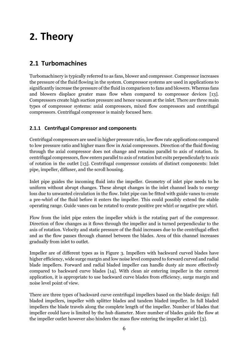
2. Theory

2.1 Turbomachines

Turbomachinery is typically referred to as fans, blower and compressor. Compressor increases

the pressure of the fluid flowing in the system. Compressor systems are used in applications to

significantly increase the pressure of the fluid in comparison to fans and blowers. Whereas fans

and blowers displace greater mass flow when compared to compressor devices [13].

Compressors create high suction pressure and hence vacuum at the inlet. There are three main

types of compressor systems: axial compressors, mixed flow compressors and centrifugal

compressors. Centrifugal compressor is mainly focused here.

2.1.1 Centrifugal Compressor and components

Centrifugal compressors are used in higher pressure ratio, low flow rate applications compared

to low pressure ratio and higher mass flow in Axial compressors. Direction of the fluid flowing

through the axial compressor does not change and remains parallel to axis of rotation. In

centrifugal compressors, flow enters parallel to axis of rotation but exits perpendicularly to axis

of rotation in the outlet [13]. Centrifugal compressor consists of distinct components: Inlet

pipe, impeller, diffuser, and the scroll housing.

Inlet pipe guides the incoming fluid into the impeller. Geometry of inlet pipe needs to be

uniform without abrupt changes. These abrupt changes in the inlet channel leads to energy

loss due to unwanted circulation in the flow. Inlet pipe can be fitted with guide vanes to create

a pre-whirl of the fluid before it enters the impeller. This could possibly extend the stable

operating range. Guide vanes can be rotated to create positive pre whirl or negative pre whirl.

Flow from the inlet pipe enters the impeller which is the rotating part of the compressor.

Direction of flow changes as it flows through the impeller and is turned perpendicular to the

axis of rotation. Velocity and static pressure of the fluid increases due to the centrifugal effect

and as the flow passes through channel between the blades. Area of this channel increases

gradually from inlet to outlet.

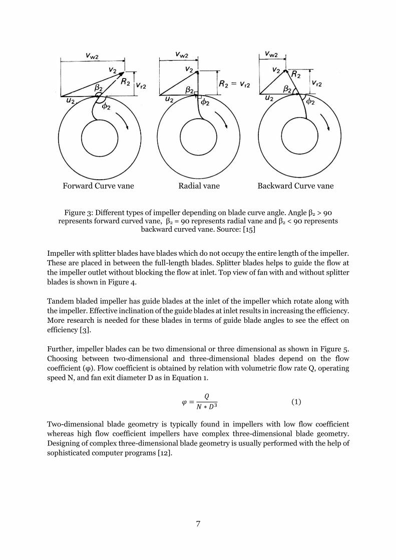
Impeller are of different types as in Figure 3. Impellers with backward curved blades have

higher efficiency, wide surge margin and low noise level compared to forward curved and radial

blade impellers. Forward and radial bladed impeller can handle dusty air more effectively

compared to backward curve blades [14]. With clean air entering impeller in the current

application, it is appropriate to use backward curve blades from efficiency, surge margin and

noise level point of view.

There are three types of backward curve centrifugal impellers based on the blade design: full

bladed impellers, impeller with splitter blades and tandem bladed impeller. In full bladed

impellers the blade travels along the complete length of the impeller. Number of blades that

impeller could have is limited by the hub diameter. More number of blades guide the flow at

the impeller outlet however also hinders the mass flow entering the impeller at inlet [3].

7

Forward Curve vane Radial vane Backward Curve vane

Figure 3: Different types of impeller depending on blade curve angle. Angle β2 > 90 represents forward curved vane, β2 = 90 represents radial vane and β2 < 90 represents

backward curved vane. Source: [15]

Impeller with splitter blades have blades which do not occupy the entire length of the impeller.

These are placed in between the full-length blades. Splitter blades helps to guide the flow at

the impeller outlet without blocking the flow at inlet. Top view of fan with and without splitter

blades is shown in Figure 4.

Tandem bladed impeller has guide blades at the inlet of the impeller which rotate along with

the impeller. Effective inclination of the guide blades at inlet results in increasing the efficiency.

More research is needed for these blades in terms of guide blade angles to see the effect on

efficiency [3].

Further, impeller blades can be two dimensional or three dimensional as shown in Figure 5.

Choosing between two-dimensional and three-dimensional blades depend on the flow

coefficient (φ). Flow coefficient is obtained by relation with volumetric flow rate Q, operating

speed N, and fan exit diameter D as in Equation 1.

𝜑 =𝑄

𝑁 ∗ 𝐷3 (1)

Two-dimensional blade geometry is typically found in impellers with low flow coefficient

whereas high flow coefficient impellers have complex three-dimensional blade geometry.

Designing of complex three-dimensional blade geometry is usually performed with the help of

sophisticated computer programs [12].

8

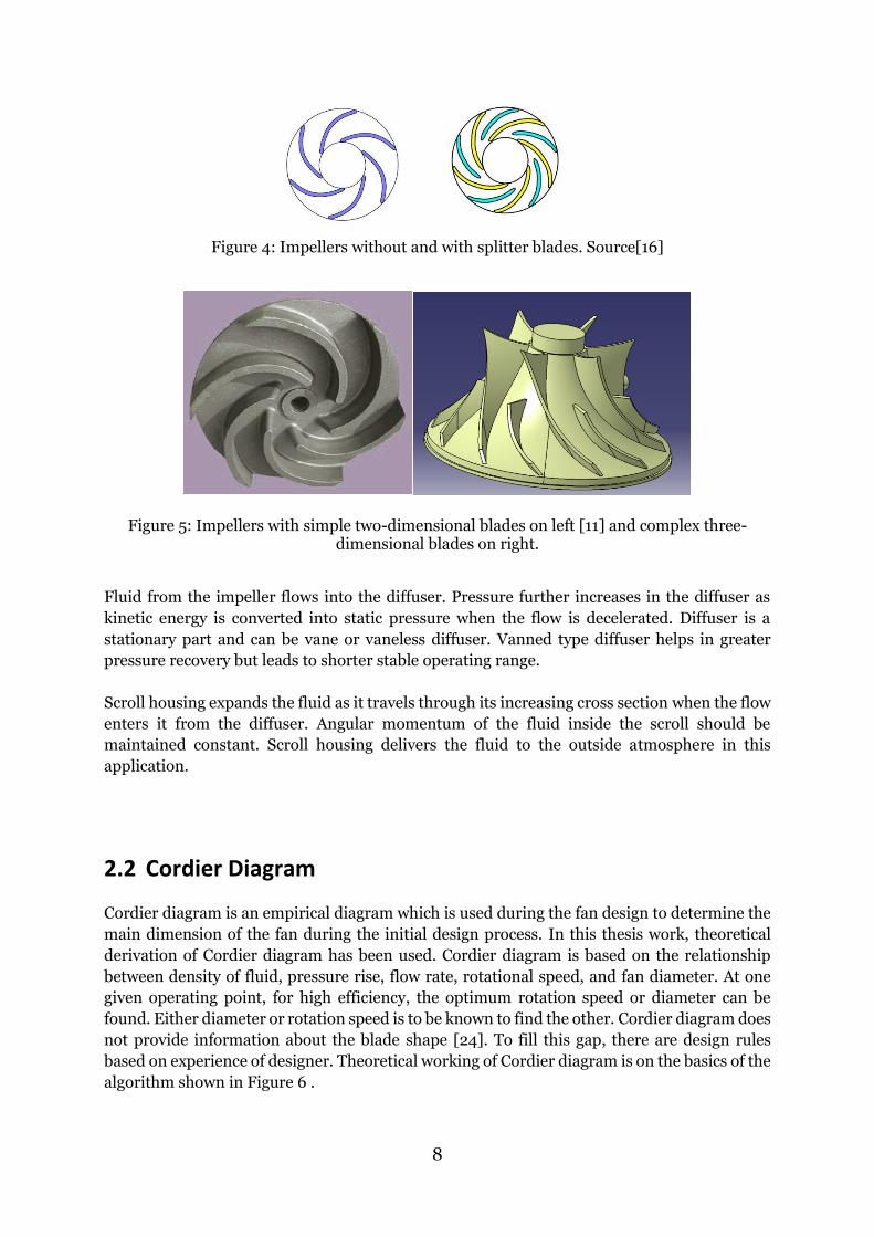
Figure 4: Impellers without and with splitter blades. Source[16]

Figure 5: Impellers with simple two-dimensional blades on left [11] and complex three- dimensional blades on right.

Fluid from the impeller flows into the diffuser. Pressure further increases in the diffuser as

kinetic energy is converted into static pressure when the flow is decelerated. Diffuser is a

stationary part and can be vane or vaneless diffuser. Vanned type diffuser helps in greater

pressure recovery but leads to shorter stable operating range.

Scroll housing expands the fluid as it travels through its increasing cross section when the flow

enters it from the diffuser. Angular momentum of the fluid inside the scroll should be

maintained constant. Scroll housing delivers the fluid to the outside atmosphere in this

application.

2.2 Cordier Diagram

Cordier diagram is an empirical diagram which is used during the fan design to determine the

main dimension of the fan during the initial design process. In this thesis work, theoretical

derivation of Cordier diagram has been used. Cordier diagram is based on the relationship

between density of fluid, pressure rise, flow rate, rotational speed, and fan diameter. At one

given operating point, for high efficiency, the optimum rotation speed or diameter can be

found. Either diameter or rotation speed is to be known to find the other. Cordier diagram does

not provide information about the blade shape [24]. To fill this gap, there are design rules

based on experience of designer. Theoretical working of Cordier diagram is on the basics of the

algorithm shown in Figure 6 .

9

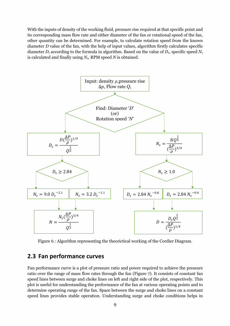
With the inputs of density of the working fluid, pressure rise required at that specific point and

its corresponding mass flow rate and either diameter of the fan or rotational speed of the fan,

other quantity can be determined. For example, to calculate rotation speed from the known

diameter D value of the fan, with the help of input values, algorithm firstly calculates specific

diameter Ds according to the formula in algorithm. Based on the value of Ds, specific speed Ns

is calculated and finally using Ns, RPM speed N is obtained.

Figure 6 : Algorithm representing the theorictical working of the Cordier Diagram.

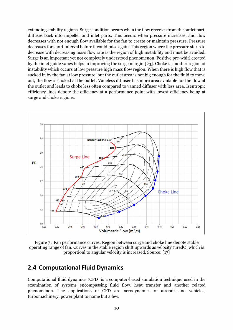
2.3 Fan performance curves

Fan performance curve is a plot of pressure ratio and power required to achieve the pressure

ratio over the range of mass flow rates through the fan (Figure 7). It consists of constant fan

speed lines between surge and choke lines on left and right side of the plot, respectively. This

plot is useful for understanding the performance of the fan at various operating points and to

determine operating range of the fan. Space between the surge and choke lines on a constant

speed lines provides stable operation. Understanding surge and choke conditions helps in

Input: density 𝜌,pressure rise ∆𝑝, Flow rate Q,

Find: Diameter ‘D’ (or)

Rotation speed ‘N’

𝐷𝑠 =𝐷(

∆𝑃𝜌 )1/4

𝑄12

𝑁𝑠 =𝑁𝑄

12

(∆𝑃𝜌 )3/4

𝐷𝑠 ≥ 2.84 𝑁𝑠 ≥ 1.0

𝑁𝑠 = 9.0 𝐷𝑠−2.1 𝑁𝑠 = 3.2 𝐷𝑠

−1.1

𝑁 =𝑁𝑠(

∆𝑃𝜌 )3/4

𝑄12

𝐷𝑠 = 2.84 𝑁𝑠−0.8 𝐷𝑠 = 2.84 𝑁𝑠

−0.4

𝐷 =𝐷𝑠𝑄

12

(∆𝑃𝜌 )1/4

10

extending stability regions. Surge condition occurs when the flow reverses from the outlet part,

diffuses back into impeller and inlet parts. This occurs when pressure increases, and flow

decreases with not enough flow available for the fan to create or maintain pressure. Pressure

decreases for short interval before it could raise again. This region where the pressure starts to

decrease with decreasing mass flow rate is the region of high instability and must be avoided.

Surge is an important yet not completely understood phenomenon. Positive pre-whirl created

by the inlet guide vanes helps in improving the surge margin [23]. Choke is another region of

instability which occurs at low pressure high mass flow region. When there is high flow that is

sucked in by the fan at low pressure, but the outlet area is not big enough for the fluid to move

out, the flow is choked at the outlet. Vaneless diffuser has more area available for the flow at

the outlet and leads to choke less often compared to vanned diffuser with less area. Isentropic

efficiency lines denote the efficiency at a performance point with lowest efficiency being at

surge and choke regions.

Figure 7 : Fan performance curves. Region between surge and choke line denote stable operating range of fan. Curves in the stable region shift upwards as velocity (uredC) which is

proportionl to angular velocity is increased. Source: [17]

2.4 Computational Fluid Dynamics

Computational fluid dynamics (CFD) is a computer-based simulation technique used in the

examination of systems encompassing fluid flow, heat transfer and another related

phenomenon. The applications of CFD are aerodynamics of aircraft and vehicles,

turbomachinery, power plant to name but a few.

11

With advancement in technology, high-performing computing hardware became affordable

and easily accessible and user operating interfaces became friendly. This paved the way to

wider use of CFD in different areas of research, which otherwise would have fallen behind other

computer-aided engineering tools due to its extreme complexity. Although, a commercial CFD

software is expensive, it has various advantages such as efficient and cost effective on new

designs; provides virtual platform to experiment and study systems which would otherwise be

impossible practically.

2.4.1 Governing equations

All the flow physics in CFD is directly or indirectly represented by the fundamental governing equations:

• Continuity equation – Mass is conserved

• Momentum equations – Newton’s second law

• Energy equation – Energy is conserved

Continuity equation is given by Equation 2.

𝜕𝜌

𝜕𝑡 +

𝜕(𝜌𝑢𝑖)

𝜕𝑥𝑖= 0

(2)

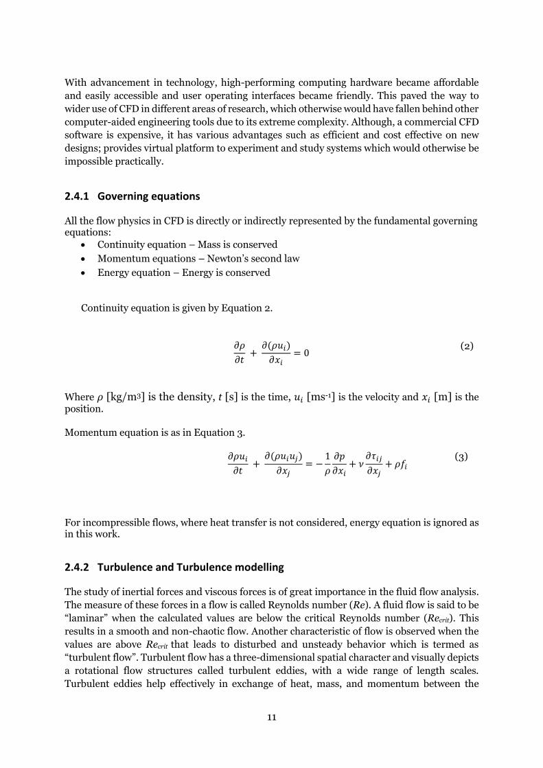
Where 𝜌 [kg/m3] is the density, t [s] is the time, 𝑢𝑖 [ms-1] is the velocity and 𝑥𝑖 [m] is the position. Momentum equation is as in Equation 3.

𝜕𝜌𝑢𝑖

𝜕𝑡 +

𝜕(𝜌𝑢𝑖𝑢𝑗)

𝜕𝑥𝑗= −

1

𝜌

𝜕𝑝

𝜕𝑥𝑖+ 𝜈

𝜕𝜏𝑖𝑗

𝜕𝑥𝑗+ 𝜌𝑓𝑖

(3)

For incompressible flows, where heat transfer is not considered, energy equation is ignored as in this work.

2.4.2 Turbulence and Turbulence modelling

The study of inertial forces and viscous forces is of great importance in the fluid flow analysis.

The measure of these forces in a flow is called Reynolds number (Re). A fluid flow is said to be

“laminar” when the calculated values are below the critical Reynolds number (Recrit). This

results in a smooth and non-chaotic flow. Another characteristic of flow is observed when the

values are above Recrit that leads to disturbed and unsteady behavior which is termed as

“turbulent flow”. Turbulent flow has a three-dimensional spatial character and visually depicts

a rotational flow structures called turbulent eddies, with a wide range of length scales.

Turbulent eddies help effectively in exchange of heat, mass, and momentum between the

12

particles of fluid. A phenomenon known as “vortex stretching” allows large turbulent eddies to

interact and exchange energy with the mean flow.

The ‘large eddy’ Reynolds number Rel is dominated by inertia effects rather than viscous

effects. This is evident because the magnitude of large eddy Reynolds number Rel = UL/v

(where U and L are the characteristic velocity and characteristic length of large eddies

respectively) is large in all turbulent flows and represents at least about Re=UL/v (where U

and L are the velocity scale and length scale of mean flow respectively) in terms of magnitude

and Re by itself is large. Large eddies are said to be anisotropic.

On the other hand, larger eddies hands down kinetic energy to progressively smaller and

smaller eddies, this process is termed as “energy cascade”. The Reynolds number Reη of

smallest eddies is based on their characteristic length η and characteristic velocity ν, Reη =νη/v,

equivalent to 1 where for the smallest scales present in a turbulent flow, the inertia and viscous

effects are equal, and these scales can be called “Kolmogorov microscales” [2]. Smaller eddies

are direction-independent, therefore are isotropic.

Turbulence Modeling

Turbulence is captured in different scales by different turbulence models. In CFD simulations

there is trade-off between solution accuracy and computational cost. Direct numerical

simulation (DNS) models capture entire turbulence scales. It requires very high computational

power. Large Eddy Simulation (LES) is more affordable model but still requires high computer

power. With LES a space filter is applied to the Navier-Stokes equations to keep the larger

scales. So, the larger eddies are resolved and the smaller eddies (those smaller than the size of

the grid) are modeled according to a sub-grid scales (SGS) model.

RANS turbulence modelling is based on Reynolds Averaged, Navier-Stokes equations. This a

simple way to handle turbulence and can model entire turbulent scale range. This is the most

common model used in the industry as it is faster, and one can achieve reliable results. Velocity

is decomposed into time averaged part and fluctuating point and is used in Navier-Stokes

equation to handle the turbulence in the RANS.

2.4.3 Wall region

When experimenting on flow behavior in the presence of solid boundary, the turbulence

structures are not the same as in free turbulent flows. This being said, the flow far away from

the wall is inertial dominated whereas the flow close to the wall is viscous dominated.

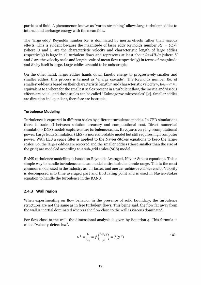
For flow close to the wall, the dimensional analysis is given by Equation 4. This formula is

called “velocity-defect law”.

𝑢+ =

𝑈

𝑢𝜏= 𝑓 (

𝜌𝑢𝜏𝑦

𝜇) = 𝑓(𝑦+)

(4)

13

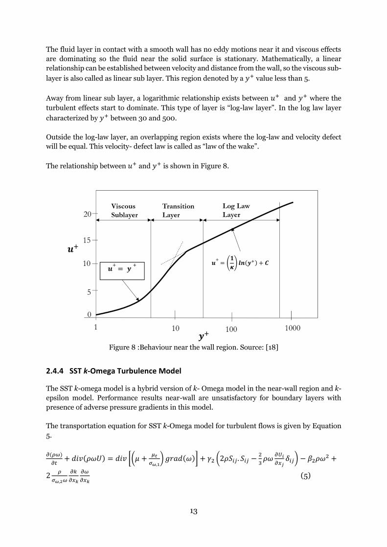
The fluid layer in contact with a smooth wall has no eddy motions near it and viscous effects

are dominating so the fluid near the solid surface is stationary. Mathematically, a linear

relationship can be established between velocity and distance from the wall, so the viscous sub-

layer is also called as linear sub layer. This region denoted by a 𝑦+ value less than 5.

Away from linear sub layer, a logarithmic relationship exists between 𝑢+ and 𝑦+ where the

turbulent effects start to dominate. This type of layer is “log-law layer”. In the log law layer

characterized by 𝑦+ between 30 and 500.

Outside the log-law layer, an overlapping region exists where the log-law and velocity defect

will be equal. This velocity- defect law is called as “law of the wake”.

The relationship between 𝑢+ and 𝑦+ is shown in Figure 8.

Figure 8 :Behaviour near the wall region. Source: [18]

2.4.4 SST k-Omega Turbulence Model

The SST k-omega model is a hybrid version of k- Omega model in the near-wall region and k-

epsilon model. Performance results near-wall are unsatisfactory for boundary layers with

presence of adverse pressure gradients in this model.

The transportation equation for SST k-Omega model for turbulent flows is given by Equation

5.

𝜕(𝜌𝜔)

𝜕𝑡+ 𝑑𝑖𝑣(𝜌𝜔𝑈) = 𝑑𝑖𝑣 [(𝜇 +

𝜇𝑡

𝜎𝜔,1) 𝑔𝑟𝑎𝑑(𝜔)] + 𝛾2 (2𝜌𝑆𝑖𝑗. 𝑆𝑖𝑗 −

2

3𝜌𝜔

𝜕𝑈𝑖

𝜕𝑥𝑗𝛿𝑖𝑗) − 𝛽2𝜌𝜔2 +

2𝜌

𝜎𝜔,2𝜔

𝜕𝑘

𝜕𝑥𝑘

𝜕𝜔

𝜕𝑥𝑘 (5)

14

Menter suggested the hybrid model by revising model constants, introducing blending

functions to achieve smooth transition between standard k-epsilon model and k-Omega model

in the near wall region, limiters to limit the performance of the flow with adverse pressure

gradients and build-up of turbulence in stagnation regions. This model is called Menter SST k-

Omega model

2.4.5 Limitations with turbulence modelling

Steady state simulations performed in this thesis with SST k-omega model cannot capture the

time dependent variations. All the time-dependent terms in the equations are forced to zero.

It is impossible to capture the effects like surge with this model as it is highly time dependent

phenomenon. RANS models behave isotropically, and model entire turbulence range and

scales are not resolved. DES and LES model can resolve large eddies in a better way compared

to RANS. Also, RANS models fail to capture large separations. Despite these limitations with

RANS model, it is proven to work very well at the best efficiency point and is used in industry

today to get quick reliable results.

15

3. Method

Thesis work method has been divided into two parts, firstly, to design a base model having

performance close to the required curved as in Figure 2. Next, to conduct the parametric

analysis by varying each parameter individually in the base model. This chapter contains

extensive description of each of these parts.

3.1 Fan Design

This section briefly explains the steps undertaken to determine the parametric model and

design of the fan. The performance requisite for which the turbo impeller and its housing was

to be designed was discussed at the company at which this thesis work was carried out. The fan

to be designed during this thesis needed to create suction of around 20 kPa at air flow rate of

around 75 m3/h and at around 300 m3/h, the fan should be able to displace the fluid at around

zero suction pressure.

Design of fan is limited by cost and ease of manufacturing of the component. Dimensional

constrains to place the fan into machine will also limit the design. As a first step, the

dimensional constraints and material of the fan was discussed with the company. Different fan

geometries, their performance is reviewed in literatures in addition to reviewing fan models

available at the company.

The initial geometry of the fan and its housing unit was modelled in a 3D modelling software,

CATIA V5, based on the knowledge gained from reviewing various fan geometries. Backward

curved centrifugal fan with splitter blades is modelled. The details of geometry are further

explained under the section 3.2.

The fan developed during the thesis was decided to be run on brushless motor in which rotation

speed can be easily controlled compared to brushed motors. So, the next step involved

performing CFD simulation on the initial geometry at several RPM speed of motor. To

determine an approximate RPM value, considerations of the performance requirement,

dimensional constraints, the RPM speed of existing motors at the company and simulations at

several rotation speeds, resulted in selecting motor speed of 34000 RPM.

By setting the rotational speed of motor constant (which is equal to 34000) in further

simulations, more simulations were performed by changing the design of the fan and housing.

Approximate value of the fan diameter is obtained with help of Cordier diagram. This step also

included addition of new elements like inlet vanes to analyze its effect on performance. This

step was conducted mainly to get the performance of the fan model closer to the required

values, and to help select the parameters required for the parametric study, explained further

under section 3.3. Knowledge from experienced colleagues supported during this process to

reduce number of simulations performed and come closer to the performance requirements

quicker.

16

The fan geometry with performance proximity to the performance requisite was selected as the

‘base geometry’ for further parametric analysis.

3.2 Geometry

Complete simulation geometry is modelled in CAD software CATIA V5 and imported into

commercial CFD software Star CCM+ version 2019.10.3. The simulation geometry is modeled

with necessary tolerances such as the clearance between the impeller and the housing around

it, from a manufacturability point of view. Pressure loss due to filters at inlet of the fan is

neglected during development phase to simplify the work. There is variation of pressure loss

as filter clogs up is neglected during this work. The complete computational domain is shown

in Figure 9. The impeller modeled is a backward curve with complex three-dimensional blades

and splitter blade as in Figure 10.

Figure 9 :Complete computational domain. Arrow directions indicate the entry and exit of the

flow.

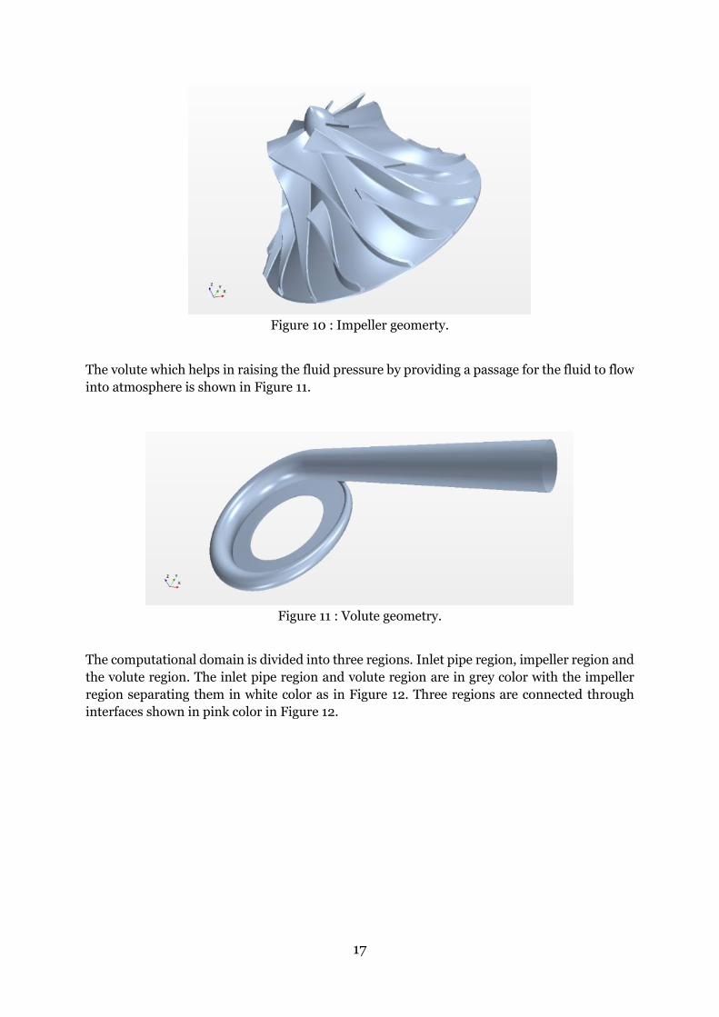
17

Figure 10 : Impeller geomerty.

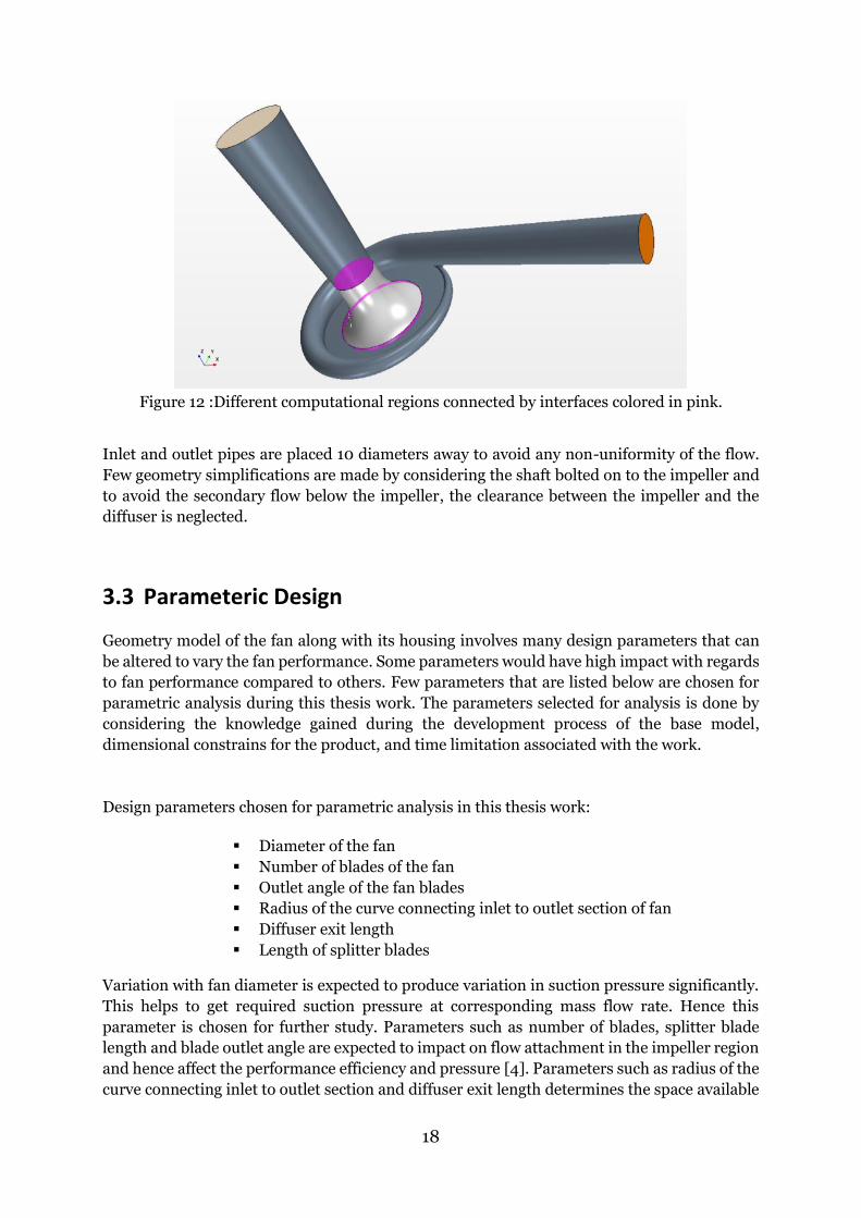
The volute which helps in raising the fluid pressure by providing a passage for the fluid to flow

into atmosphere is shown in Figure 11.

Figure 11 : Volute geometry.

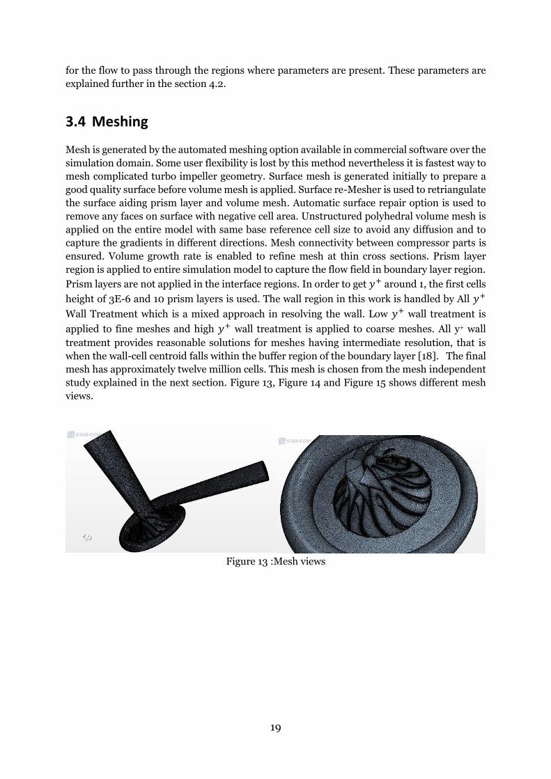
The computational domain is divided into three regions. Inlet pipe region, impeller region and

the volute region. The inlet pipe region and volute region are in grey color with the impeller

region separating them in white color as in Figure 12. Three regions are connected through

interfaces shown in pink color in Figure 12.

18

Figure 12 :Different computational regions connected by interfaces colored in pink.

Inlet and outlet pipes are placed 10 diameters away to avoid any non-uniformity of the flow.

Few geometry simplifications are made by considering the shaft bolted on to the impeller and

to avoid the secondary flow below the impeller, the clearance between the impeller and the

diffuser is neglected.

3.3 Parameteric Design

Geometry model of the fan along with its housing involves many design parameters that can

be altered to vary the fan performance. Some parameters would have high impact with regards

to fan performance compared to others. Few parameters that are listed below are chosen for

parametric analysis during this thesis work. The parameters selected for analysis is done by

considering the knowledge gained during the development process of the base model,

dimensional constrains for the product, and time limitation associated with the work.

Design parameters chosen for parametric analysis in this thesis work:

▪ Diameter of the fan

▪ Number of blades of the fan

▪ Outlet angle of the fan blades

▪ Radius of the curve connecting inlet to outlet section of fan

▪ Diffuser exit length

▪ Length of splitter blades

Variation with fan diameter is expected to produce variation in suction pressure significantly.

This helps to get required suction pressure at corresponding mass flow rate. Hence this

parameter is chosen for further study. Parameters such as number of blades, splitter blade

length and blade outlet angle are expected to impact on flow attachment in the impeller region

and hence affect the performance efficiency and pressure [4]. Parameters such as radius of the

curve connecting inlet to outlet section and diffuser exit length determines the space available

19

for the flow to pass through the regions where parameters are present. These parameters are

explained further in the section 4.2.

3.4 Meshing

Mesh is generated by the automated meshing option available in commercial software over the

simulation domain. Some user flexibility is lost by this method nevertheless it is fastest way to

mesh complicated turbo impeller geometry. Surface mesh is generated initially to prepare a

good quality surface before volume mesh is applied. Surface re-Mesher is used to retriangulate

the surface aiding prism layer and volume mesh. Automatic surface repair option is used to

remove any faces on surface with negative cell area. Unstructured polyhedral volume mesh is

applied on the entire model with same base reference cell size to avoid any diffusion and to

capture the gradients in different directions. Mesh connectivity between compressor parts is

ensured. Volume growth rate is enabled to refine mesh at thin cross sections. Prism layer

region is applied to entire simulation model to capture the flow field in boundary layer region.

Prism layers are not applied in the interface regions. In order to get 𝑦+ around 1, the first cells

height of 3E-6 and 10 prism layers is used. The wall region in this work is handled by All 𝑦+

Wall Treatment which is a mixed approach in resolving the wall. Low 𝑦+ wall treatment is

applied to fine meshes and high 𝑦+ wall treatment is applied to coarse meshes. All y+ wall

treatment provides reasonable solutions for meshes having intermediate resolution, that is

when the wall-cell centroid falls within the buffer region of the boundary layer [18]. The final

mesh has approximately twelve million cells. This mesh is chosen from the mesh independent

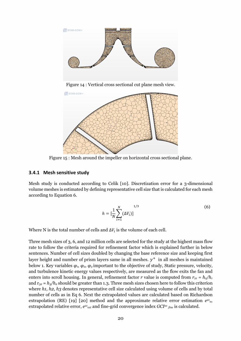
study explained in the next section. Figure 13, Figure 14 and Figure 15 shows different mesh

views.

Figure 13 :Mesh views

20

Figure 14 : Vertical cross sectional cut plane mesh view.

Figure 15 : Mesh around the impeller on horizontal cross sectional plane.

3.4.1 Mesh sensitive study

Mesh study is conducted according to Celik [10]. Discretization error for a 3-dimensional

volume meshes is estimated by defining representative cell size that is calculated for each mesh

according to Equation 6.

ℎ = [1

𝑁∑(∆𝑉𝑖)]

𝑁

𝑖=1

1/3

(6)

Where N is the total number of cells and ∆𝑉𝑖 is the volume of each cell.

Three mesh sizes of 3, 6, and 12 million cells are selected for the study at the highest mass flow

rate to follow the criteria required for refinement factor which is explained further in below

sentences. Number of cell sizes doubled by changing the base reference size and keeping first

layer height and number of prism layers same in all meshes. 𝑦+ in all meshes is maintained

below 1. Key variables φ1, φ2, φ3 important to the objective of study, Static pressure, velocity,

and turbulence kinetic energy values respectively, are measured as the flow exits the fan and

enters into scroll housing. In general, refinement factor r value is computed from r21 = h2/h1

and r32 = h3/h2 should be greater than 1.3. Three mesh sizes chosen here to follow this criterion

where h1, h2, h3 denotes representative cell size calculated using volume of cells and by total

number of cells as in Eq 6. Next the extrapolated values are calculated based on Richardson

extrapolation (RE) [19] [20] method and the approximate relative error estimation e21a,

extrapolated relative error, e21ext and fine-grid convergence index GCI21 fine is calculated.

21

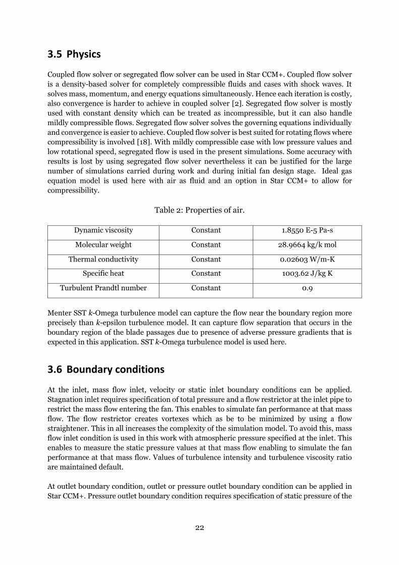
Table 1: Mesh sensitive study for different variables at highest mass flow

φ =Pressure φ =Velocity φ =TKE

M1, M2, M3 12M, 6M, 3M

h1, h2, h3 8.94E-4, 1.28E-3, 1.90E-3

r21 1.427 1.427 1.427

r32 1.489 1.489 1.489

φ1 152.65 71.69 26.06

φ 2 153.21 71.78 26.34

φ 3 155.23 72.78 27.87

φ 21ext 152.39 71.92 25.98

p 3.10 5.95 4.10

e21a 0.36% 0.12% 1.08%

e21ext 0.17% 0.32% 0.31%

GCI21 fine 0.22% 0.021% 0.41%

The Grid convergence Index (GCI) calculated by extrapolating the variables based on RE, with

pressure, velocity, TKE values from 12 Million mesh size to higher cell elements is very less.

Hence can be concluded 12 Million mesh elements is reasonable for this study.

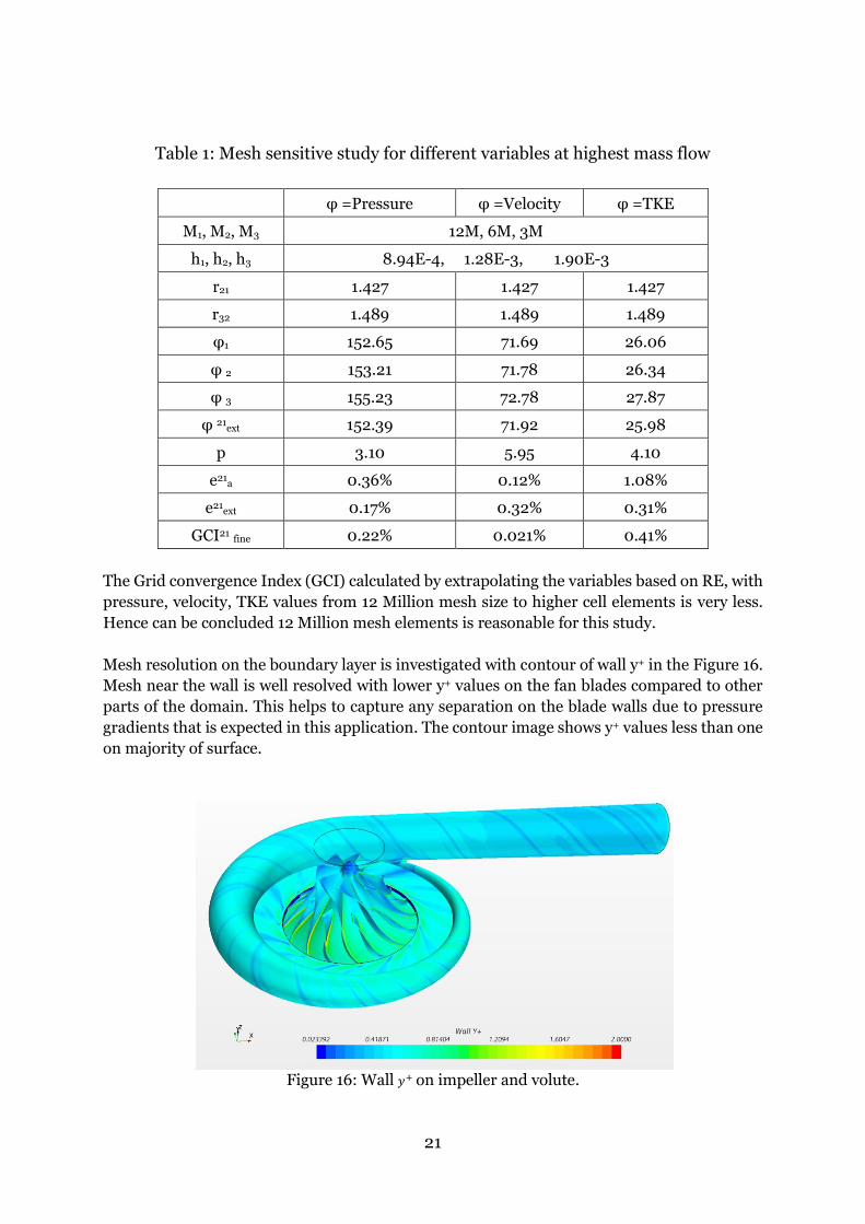
Mesh resolution on the boundary layer is investigated with contour of wall y+ in the Figure 16.

Mesh near the wall is well resolved with lower y+ values on the fan blades compared to other

parts of the domain. This helps to capture any separation on the blade walls due to pressure

gradients that is expected in this application. The contour image shows y+ values less than one

on majority of surface.

Figure 16: Wall 𝑦+ on impeller and volute.

22

3.5 Physics

Coupled flow solver or segregated flow solver can be used in Star CCM+. Coupled flow solver

is a density-based solver for completely compressible fluids and cases with shock waves. It

solves mass, momentum, and energy equations simultaneously. Hence each iteration is costly,

also convergence is harder to achieve in coupled solver [2]. Segregated flow solver is mostly

used with constant density which can be treated as incompressible, but it can also handle

mildly compressible flows. Segregated flow solver solves the governing equations individually

and convergence is easier to achieve. Coupled flow solver is best suited for rotating flows where

compressibility is involved [18]. With mildly compressible case with low pressure values and

low rotational speed, segregated flow is used in the present simulations. Some accuracy with

results is lost by using segregated flow solver nevertheless it can be justified for the large

number of simulations carried during work and during initial fan design stage. Ideal gas

equation model is used here with air as fluid and an option in Star CCM+ to allow for

compressibility.

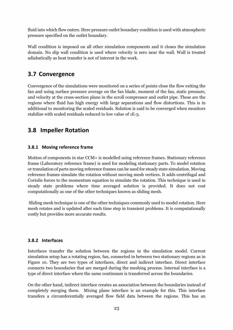
Table 2: Properties of air.

Dynamic viscosity Constant 1.8550 E-5 Pa-s

Molecular weight Constant 28.9664 kg/k mol

Thermal conductivity Constant 0.02603 W/m-K

Specific heat Constant 1003.62 J/kg K

Turbulent Prandtl number Constant 0.9

Menter SST k-Omega turbulence model can capture the flow near the boundary region more

precisely than k-epsilon turbulence model. It can capture flow separation that occurs in the

boundary region of the blade passages due to presence of adverse pressure gradients that is

expected in this application. SST k-Omega turbulence model is used here.

3.6 Boundary conditions

At the inlet, mass flow inlet, velocity or static inlet boundary conditions can be applied.

Stagnation inlet requires specification of total pressure and a flow restrictor at the inlet pipe to

restrict the mass flow entering the fan. This enables to simulate fan performance at that mass

flow. The flow restrictor creates vortexes which as be to be minimized by using a flow

straightener. This in all increases the complexity of the simulation model. To avoid this, mass

flow inlet condition is used in this work with atmospheric pressure specified at the inlet. This

enables to measure the static pressure values at that mass flow enabling to simulate the fan

performance at that mass flow. Values of turbulence intensity and turbulence viscosity ratio

are maintained default.

At outlet boundary condition, outlet or pressure outlet boundary condition can be applied in

Star CCM+. Pressure outlet boundary condition requires specification of static pressure of the

23

fluid into which flow enters. Here pressure outlet boundary condition is used with atmospheric

pressure specified on the outlet boundary.

Wall condition is imposed on all other simulation components and it closes the simulation

domain. No slip wall condition is used where velocity is zero near the wall. Wall is treated

adiabatically as heat transfer is not of interest in the work.

3.7 Convergence

Convergence of the simulations were monitored on a series of points close the flow exiting the

fan and using surface pressure average on the fan blade, moment of the fan, static pressure,

and velocity at the cross-section plane in the scroll compressor and outlet pipe. These are the

regions where fluid has high energy with large separations and flow distortions. This is in

additional to monitoring the scaled residuals. Solution is said to be converged when monitors

stabilize with scaled residuals reduced to low value of 1E-5.

3.8 Impeller Rotation

3.8.1 Moving reference frame

Motion of components in star CCM+ is modelled using reference frames. Stationary reference

frame (Laboratory reference frame) is used for modeling stationary parts. To model rotation

or translation of parts moving reference frames can be used for steady state simulation. Moving

reference frames simulate the rotation without moving mesh vertices. It adds centrifugal and

Coriolis forces to the momentum equation to simulate the rotation. This technique is used in

steady state problems where time averaged solution is provided. It does not cost

computationally as one of the other techniques known as sliding mesh.

Sliding mesh technique is one of the other techniques commonly used to model rotation. Here

mesh rotates and is updated after each time step in transient problems. It is computationally

costly but provides more accurate results.

3.8.2 Interfaces

Interfaces transfer the solution between the regions in the simulation model. Current

simulation setup has a rotating region, fan, connected in between two stationary regions as in

Figure 10. They are two types of interfaces, direct and indirect interface. Direct interface

connects two boundaries that are merged during the meshing process. Internal interface is a

type of direct interface where the same continuum is transferred across the boundaries.

On the other hand, indirect interface creates an association between the boundaries instead of

completely merging them. Mixing plane interface is an example for this. This interface

transfers a circumferentially averaged flow field data between the regions. This has an

24

advantage that it can mitigate the error caused by moving reference frame, but this cannot

capture wakes due to the averaging. This is mainly used in steady state simulation of multistage

turbomachinery. This thesis work uses direct internal interface.

25

4. Results

This chapter shows the results in two parts, first of the base model, its performance curve

with flow contours and finally the results from the parametric study.

4.1 Base Geometry

4.1.1 Performance Curve

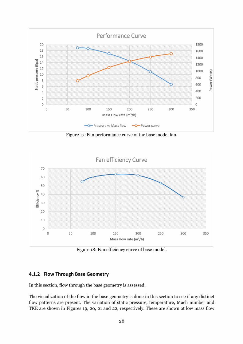
The performance of base model is simulated at six different mass flow rates at single rotation

speed of the motor (34000 RPM) that was chosen. The performance maps showing suction

static pressure, power consumption against different mass flow rates is plotted in Figure 17.

The performance curve in Figure 17 looks different to one in Figure 7 as in Figure 7, fan is

simulated at different velocities (uredC) which is proportional to angular velocity. But in Figure

17, fan is simulated only at one rotational speed. The decrease in suction pressure with increase

in mass flow rate can be observed which is normal. Pressure curve shows a gradual decrease in

pressure with increase in mass flow rate and no sudden changes are seen. Highest suction

pressure is around 19 kPa at the lowest mass flow rate simulated i.e. 75 m3/h. Lowest suction

pressure is around 6 kPa at highest mass flow rate simulated – 300 m3/h. Natural increase in

power consumption of the fan with the increase in mass flow rate due to increase in fan

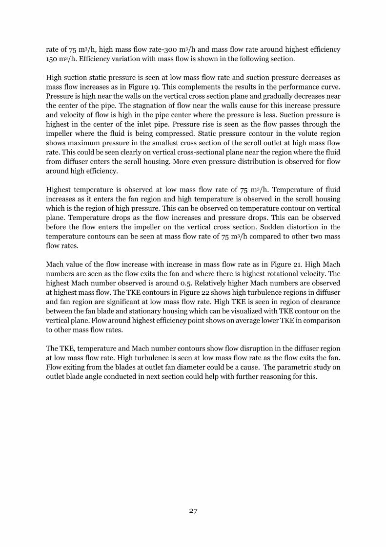
moment is observed with the power curve. The efficiency curve at different mass flow rates is

shown in Figure 18.

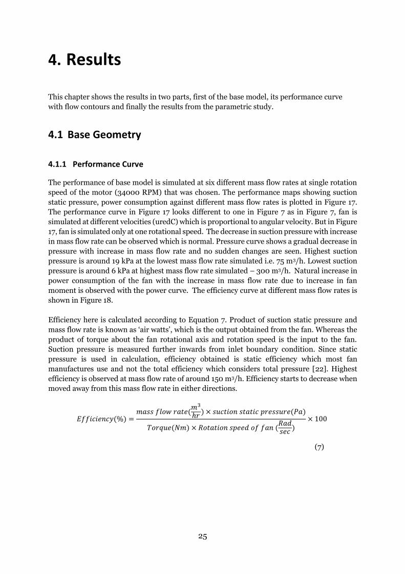
Efficiency here is calculated according to Equation 7. Product of suction static pressure and

mass flow rate is known as ‘air watts’, which is the output obtained from the fan. Whereas the

product of torque about the fan rotational axis and rotation speed is the input to the fan.

Suction pressure is measured further inwards from inlet boundary condition. Since static

pressure is used in calculation, efficiency obtained is static efficiency which most fan

manufactures use and not the total efficiency which considers total pressure [22]. Highest

efficiency is observed at mass flow rate of around 150 m3/h. Efficiency starts to decrease when

moved away from this mass flow rate in either directions.

𝐸𝑓𝑓𝑖𝑐𝑖𝑒𝑛𝑐𝑦(%) =𝑚𝑎𝑠𝑠 𝑓𝑙𝑜𝑤 𝑟𝑎𝑡𝑒(

𝑚3

ℎ𝑟) × 𝑠𝑢𝑐𝑡𝑖𝑜𝑛 𝑠𝑡𝑎𝑡𝑖𝑐 𝑝𝑟𝑒𝑠𝑠𝑢𝑟𝑒(𝑃𝑎)

𝑇𝑜𝑟𝑞𝑢𝑒(𝑁𝑚) × 𝑅𝑜𝑡𝑎𝑡𝑖𝑜𝑛 𝑠𝑝𝑒𝑒𝑑 𝑜𝑓 𝑓𝑎𝑛 (𝑅𝑎𝑑𝑠𝑒𝑐 )

× 100

(7)

26

Figure 17 :Fan performance curve of the base model fan.

Figure 18: Fan efficiency curve of base model.

4.1.2 Flow Through Base Geometry

In this section, flow through the base geometry is assessed.

The visualization of the flow in the base geometry is done in this section to see if any distinct

flow patterns are present. The variation of static pressure, temperature, Mach number and

TKE are shown in Figures 19, 20, 21 and 22, respectively. These are shown at low mass flow

0

200

400

600

800

1000

1200

1400

1600

1800

0

2

4

6

8

10

12

14

16

18

20

0 50 100 150 200 250 300 350

Po

we

r (W

atts

)

Stat

ic p

ress

ure

(K

pa)

Mass Flow rate (m3/h)

Performance Curve

Pressure vs Mass flow Power curve

0

10

20

30

40

50

60

70

0 50 100 150 200 250 300 350

Effi

cie

ncy

%

Mass Flow rate (m3/h)

Fan efficiency Curve

27

rate of 75 m3/h, high mass flow rate-300 m3/h and mass flow rate around highest efficiency

150 m3/h. Efficiency variation with mass flow is shown in the following section.

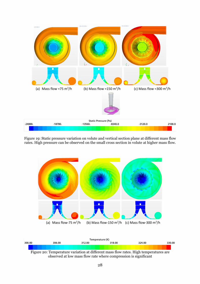
High suction static pressure is seen at low mass flow rate and suction pressure decreases as

mass flow increases as in Figure 19. This complements the results in the performance curve.

Pressure is high near the walls on the vertical cross section plane and gradually decreases near

the center of the pipe. The stagnation of flow near the walls cause for this increase pressure

and velocity of flow is high in the pipe center where the pressure is less. Suction pressure is

highest in the center of the inlet pipe. Pressure rise is seen as the flow passes through the

impeller where the fluid is being compressed. Static pressure contour in the volute region

shows maximum pressure in the smallest cross section of the scroll outlet at high mass flow

rate. This could be seen clearly on vertical cross-sectional plane near the region where the fluid

from diffuser enters the scroll housing. More even pressure distribution is observed for flow

around high efficiency.

Highest temperature is observed at low mass flow rate of 75 m3/h. Temperature of fluid

increases as it enters the fan region and high temperature is observed in the scroll housing

which is the region of high pressure. This can be observed on temperature contour on vertical

plane. Temperature drops as the flow increases and pressure drops. This can be observed

before the flow enters the impeller on the vertical cross section. Sudden distortion in the

temperature contours can be seen at mass flow rate of 75 m3/h compared to other two mass

flow rates.

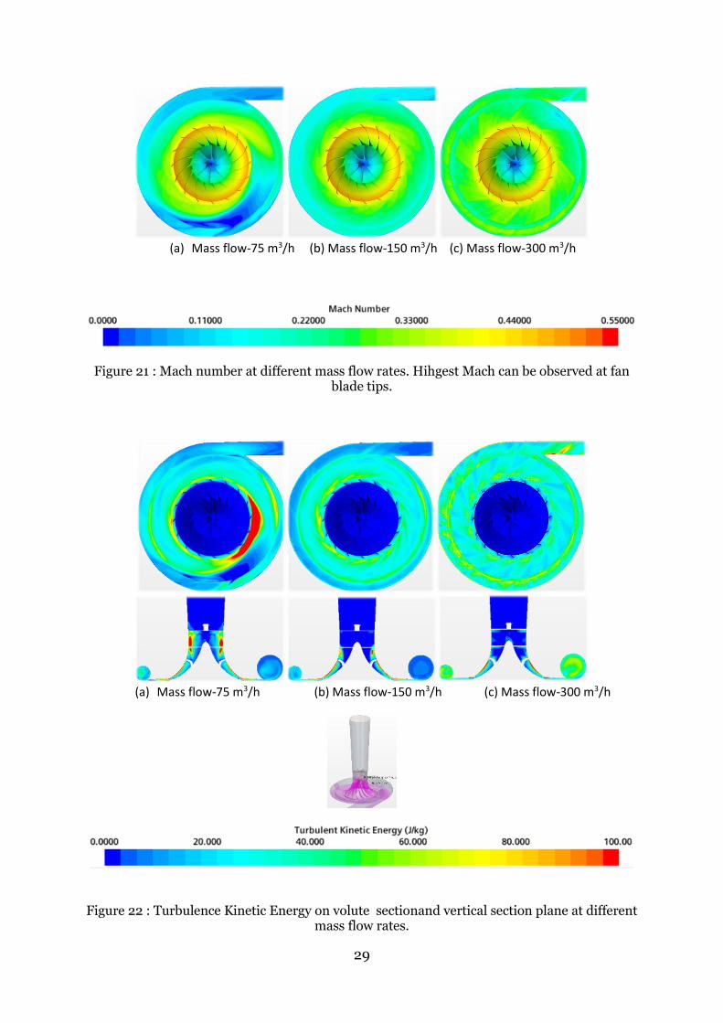
Mach value of the flow increase with increase in mass flow rate as in Figure 21. High Mach

numbers are seen as the flow exits the fan and where there is highest rotational velocity. The

highest Mach number observed is around 0.5. Relatively higher Mach numbers are observed

at highest mass flow. The TKE contours in Figure 22 shows high turbulence regions in diffuser

and fan region are significant at low mass flow rate. High TKE is seen in region of clearance

between the fan blade and stationary housing which can be visualized with TKE contour on the

vertical plane. Flow around highest efficiency point shows on average lower TKE in comparison

to other mass flow rates.

The TKE, temperature and Mach number contours show flow disruption in the diffuser region

at low mass flow rate. High turbulence is seen at low mass flow rate as the flow exits the fan.

Flow exiting from the blades at outlet fan diameter could be a cause. The parametric study on

outlet blade angle conducted in next section could help with further reasoning for this.

28

(a) Mass flow =75 m3/h (b) Mass flow =150 m3/h (c) Mass flow =300 m3/h

Figure 19: Static pressure variation on volute and vertical section plane at different mass flow rates. High pressure can be observed on the small cross section in volute at higher mass flow.

(a) Mass flow-75 m3/h (b) Mass flow-150 m3/h (c) Mass flow-300 m3/h

Figure 20: Temperature variation at different mass flow rates. High temperatures are

observed at low mass flow rate where compression is significant

29

(a) Mass flow-75 m3/h (b) Mass flow-150 m3/h (c) Mass flow-300 m3/h

Figure 21 : Mach number at different mass flow rates. Hihgest Mach can be observed at fan blade tips.

(a) Mass flow-75 m3/h (b) Mass flow-150 m3/h (c) Mass flow-300 m3/h

Figure 22 : Turbulence Kinetic Energy on volute sectionand vertical section plane at different mass flow rates.

30

4.2 Parametric study

Six fan design parameters are analyzed at two mass flow rates, 300 m3/h and at 75 m3/h which

is also simulated for the base model. The performance variance with suction static pressure

and efficiency at these two mass flow rates are presented in this section.

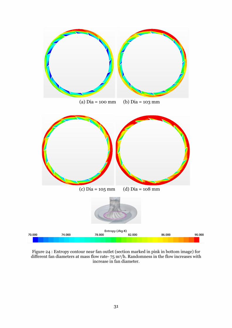
4.2.1 Fan Diameter

Static pressure and efficiency variation as the fan diameter is increased in a range of 8 mm for

two mass flows is shown in Figure 23. Suction static pressure increases as diameter gets larger

at both 75 m3/h and 300 m3/h air flow rates. Efficiency decreases with increase in diameter at

75 m3/h mass flow rate and opposite trend is seen at 300 m3/h. Figure 24 shows the entropy

comparison at 75 m3/h mass flow as it exits from fans with varied diameters. Entropy gives

amount of disorder or randomness in the flow. As the fan diameter increases, greater disorder

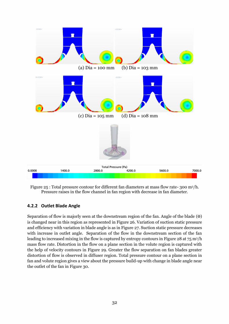
in the flow can be observed leading to decrease in efficiency. Figure 25 shows the total pressure

contour on a vertical plane in fan and volute section at mass flow rate of 300 m3/h. Pressure

build up at the fan region indicates the blocked flow. Greater pressure build up can be seen in

fans with small diameter.

Figure 23 : Variation of Static pressure and Efficiency with change in Fan diameter.

50

52

54

56

16

17

18

19

20

21

100 103 105 108

Effi

cien

cy %

Stat

ic p

ress

ure

(K

Pa)

Diameter (mm)

Mass flow rate-75 m3/h

20

25

30

35

40

45

50

3

5

7

9

11

13

100 103 105 108

Effi

cien

cy %

Stat

ic p

ress

ure

(K

Pa)

Diameter (mm)

Mass flow rate- 300 m3/h

31

(a) Dia = 100 mm (b) Dia = 103 mm

(c) Dia = 105 mm (d) Dia = 108 mm

Figure 24 : Entropy contour near fan outlet (section marked in pink in bottom image) for different fan diameters at mass flow rate- 75 m3/h. Randomness in the flow increases with

increase in fan diameter.

32

(a) Dia = 100 mm (b) Dia = 103 mm

(c) Dia = 105 mm (d) Dia = 108 mm

Figure 25 : Total pressure contour for different fan diameters at mass flow rate- 300 m3/h. Pressure raises in the flow channel in fan region with decrease in fan diameter.

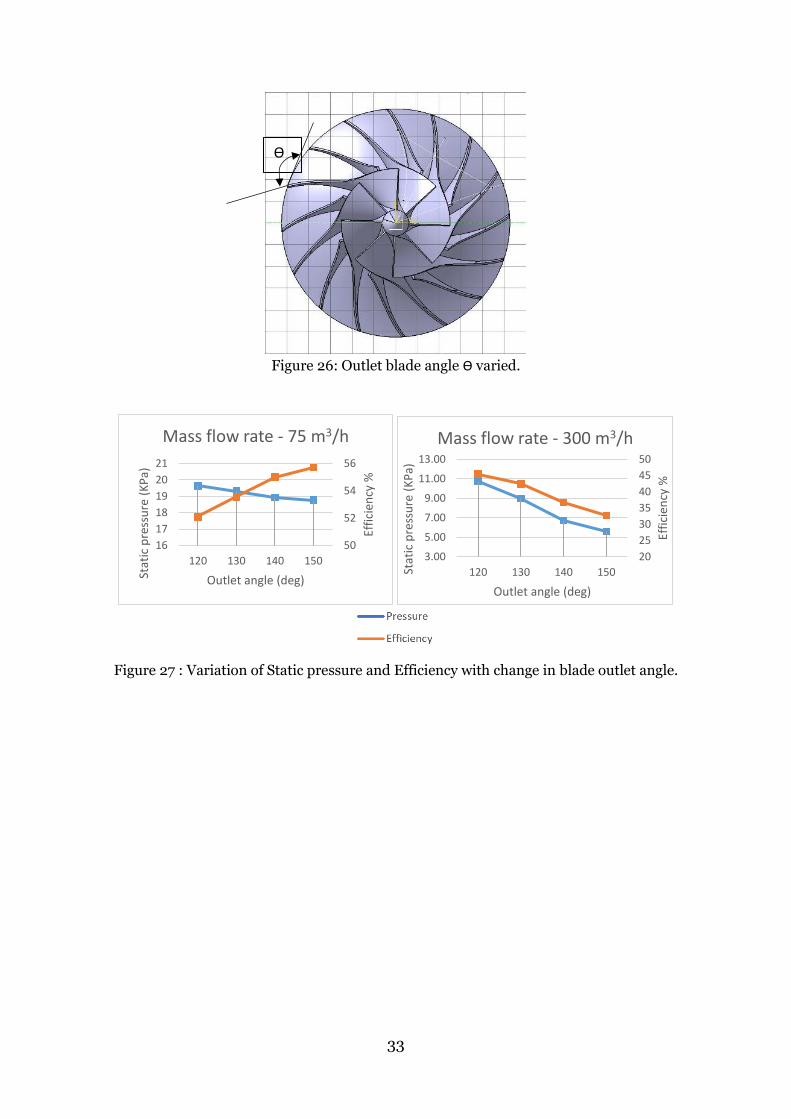
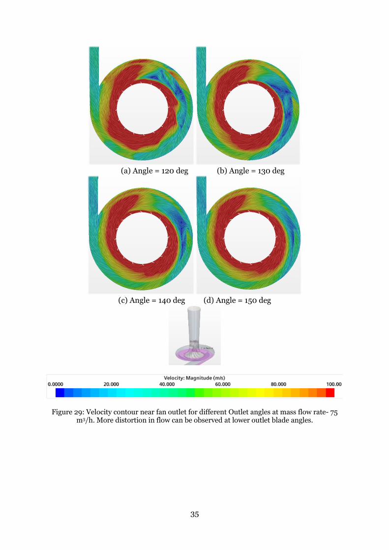
4.2.2 Outlet Blade Angle

Separation of flow is majorly seen at the downstream region of the fan. Angle of the blade (ϴ)

is changed near in this region as represented in Figure 26. Variation of suction static pressure

and efficiency with variation in blade angle is as in Figure 27. Suction static pressure decreases

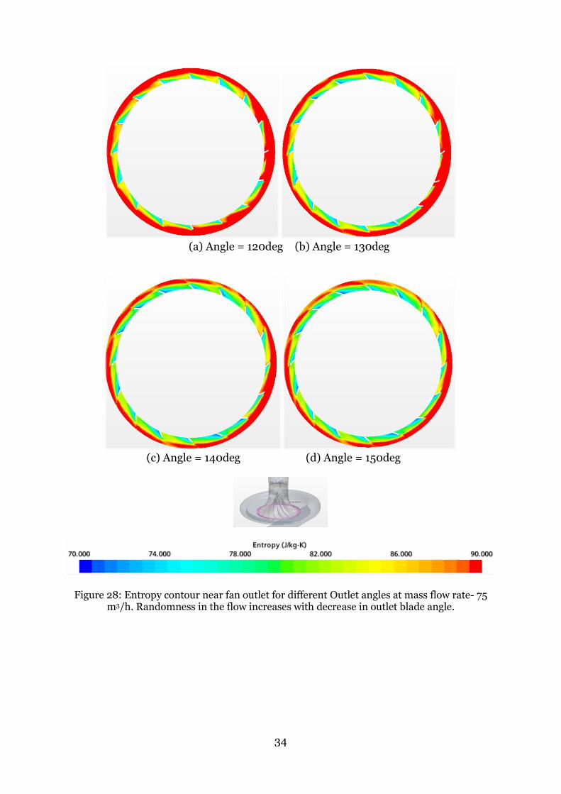
with increase in outlet angle. Separation of the flow in the downstream section of the fan

leading to increased mixing in the flow is captured by entropy contours in Figure 28 at 75 m3/h

mass flow rate. Distortion in the flow on a plane section in the volute region is captured with

the help of velocity contours in Figure 29. Greater the flow separation on fan blades greater

distortion of flow is observed in diffuser region. Total pressure contour on a plane section in

fan and volute region gives a view about the pressure build-up with change in blade angle near

the outlet of the fan in Figure 30.

33

Figure 26: Outlet blade angle ϴ varied.

Figure 27 : Variation of Static pressure and Efficiency with change in blade outlet angle.

50

52

54

56

16

17

18

19

20

21

120 130 140 150

Effi

cien

cy %

Stat

ic p

ress

ure

(K

Pa)

Outlet angle (deg)

Mass flow rate - 75 m3/h

20

25

30

35

40

45

50

3.00

5.00

7.00

9.00

11.00

13.00

120 130 140 150

Effi

cien

cy %

Stat

ic p

ress

ure

(K

Pa)

Outlet angle (deg)

Mass flow rate - 300 m3/h

ϴ

34

(a) Angle = 120deg (b) Angle = 130deg

(c) Angle = 140deg (d) Angle = 150deg

Figure 28: Entropy contour near fan outlet for different Outlet angles at mass flow rate- 75 m3/h. Randomness in the flow increases with decrease in outlet blade angle.

35

(a) Angle = 120 deg (b) Angle = 130 deg

(c) Angle = 140 deg (d) Angle = 150 deg

Figure 29: Velocity contour near fan outlet for different Outlet angles at mass flow rate- 75 m3/h. More distortion in flow can be observed at lower outlet blade angles.

36

(a) Angle = 120 deg (b) Angle = 130 deg

(c) Angle = 140 deg (d) Angle = 150 deg

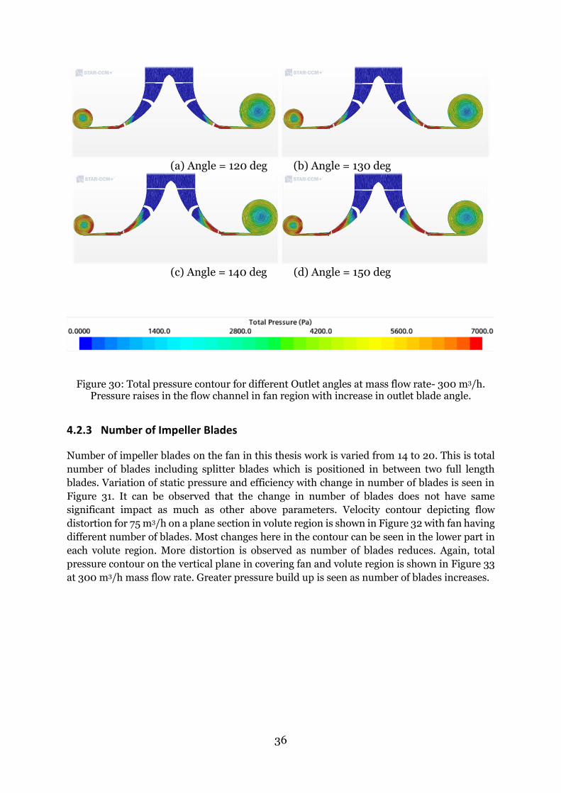
Figure 30: Total pressure contour for different Outlet angles at mass flow rate- 300 m3/h.

Pressure raises in the flow channel in fan region with increase in outlet blade angle.

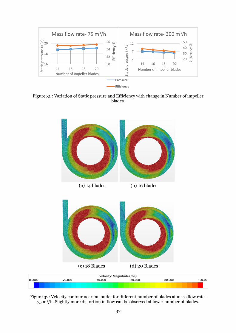
4.2.3 Number of Impeller Blades

Number of impeller blades on the fan in this thesis work is varied from 14 to 20. This is total

number of blades including splitter blades which is positioned in between two full length

blades. Variation of static pressure and efficiency with change in number of blades is seen in

Figure 31. It can be observed that the change in number of blades does not have same

significant impact as much as other above parameters. Velocity contour depicting flow

distortion for 75 m3/h on a plane section in volute region is shown in Figure 32 with fan having

different number of blades. Most changes here in the contour can be seen in the lower part in

each volute region. More distortion is observed as number of blades reduces. Again, total

pressure contour on the vertical plane in covering fan and volute region is shown in Figure 33

at 300 m3/h mass flow rate. Greater pressure build up is seen as number of blades increases.

37

Figure 31 : Variation of Static pressure and Efficiency with change in Number of impeller

blades.

(a) 14 blades (b) 16 blades

(c) 18 Blades (d) 20 Blades

Figure 32: Velocity contour near fan outlet for different number of blades at mass flow rate- 75 m3/h. Slightly more distortion in flow can be observed at lower number of blades.

50

52

54

56

16

18

20

14 16 18 20

Effi

cien

cy %

Stat

ic p

ress

ure

(K

Pa)

Number of Impeller blades

Mass flow rate- 75 m3/h

20

30

40

50

2

7

12

14 16 18 20

Effi

cien

cy %

Stat

ic p

ress

ure

(K

Pa)

Number of Impeller blades

Mass flow rate- 300 m3/h

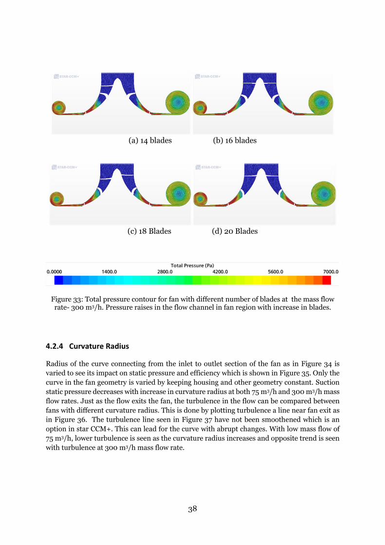
38

(a) 14 blades (b) 16 blades

(c) 18 Blades (d) 20 Blades

Figure 33: Total pressure contour for fan with different number of blades at the mass flow rate- 300 m3/h. Pressure raises in the flow channel in fan region with increase in blades.

4.2.4 Curvature Radius

Radius of the curve connecting from the inlet to outlet section of the fan as in Figure 34 is

varied to see its impact on static pressure and efficiency which is shown in Figure 35. Only the

curve in the fan geometry is varied by keeping housing and other geometry constant. Suction

static pressure decreases with increase in curvature radius at both 75 m3/h and 300 m3/h mass

flow rates. Just as the flow exits the fan, the turbulence in the flow can be compared between

fans with different curvature radius. This is done by plotting turbulence a line near fan exit as

in Figure 36. The turbulence line seen in Figure 37 have not been smoothened which is an

option in star CCM+. This can lead for the curve with abrupt changes. With low mass flow of

75 m3/h, lower turbulence is seen as the curvature radius increases and opposite trend is seen

with turbulence at 300 m3/h mass flow rate.

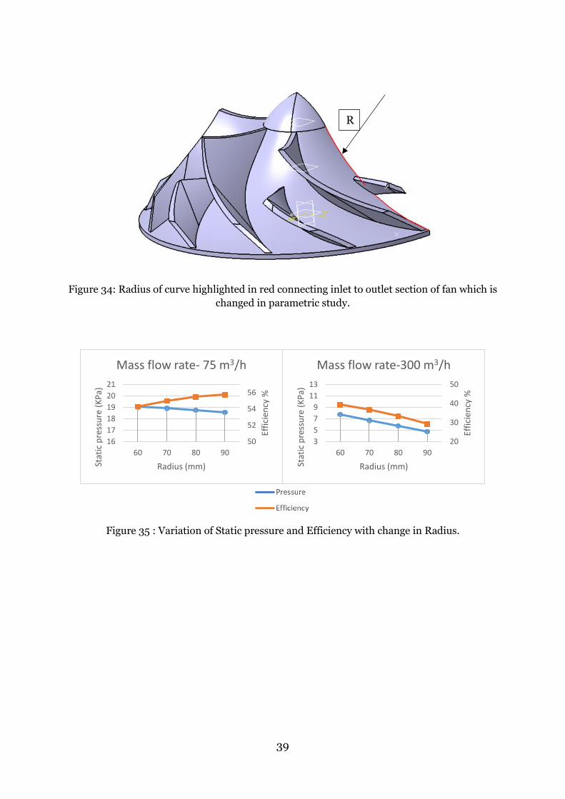
39

Figure 34: Radius of curve highlighted in red connecting inlet to outlet section of fan which is

changed in parametric study.

Figure 35 : Variation of Static pressure and Efficiency with change in Radius.

50

52

54

56

16

17

18

19

20

21

60 70 80 90

Effi

cien

cy %

Stat

ic p

ress

ure

(K

Pa)

Radius (mm)

Mass flow rate- 75 m3/h

20

30

40

50

3

5

7

9

11

13

60 70 80 90

Effi

cien

cy %

Stat

ic p

ress

ure

(K

Pa)

Radius (mm)

Mass flow rate-300 m3/h

R

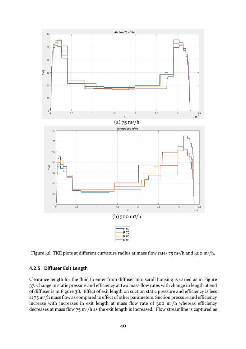
40

(a) 75 m3/h

(b) 300 m3/h

Figure 36: TKE plots at different curvature radius at mass flow rate- 75 m3/h and 300 m3/h.

4.2.5 Diffuser Exit Length

Clearance length for the fluid to enter from diffuser into scroll housing is varied as in Figure

37. Change in static pressure and efficiency at two mass flow rates with change in length at end

of diffuser is in Figure 38. Effect of exit length on suction static pressure and efficiency is less

at 75 m3/h mass flow as compared to effect of other parameters. Suction pressure and efficiency

increase with increases in exit length at mass flow rate of 300 m3/h whereas efficiency

decreases at mass flow 75 m3/h as the exit length is increased. Flow streamline is captured as

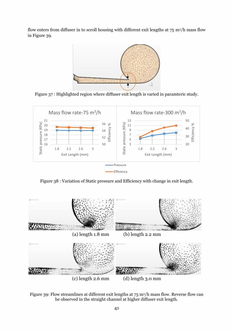
41

flow enters from diffuser in to scroll housing with different exit lengths at 75 m3/h mass flow

in Figure 39.

Figure 37 : Highlighted region where diffuser exit length is varied in paramteric study.

Figure 38 : Variation of Static pressure and Efficiency with change in exit length.

(a) length 1.8 mm (b) length 2.2 mm

(c) length 2.6 mm (d) length 3.0 mm

Figure 39: Flow streamlines at different exit lengths at 75 m3/h mass flow. Reverse flow can be observed in the straight channel at higher diffuser exit length.

50

52

54

56

16

17

18

19

20

21

1.8 2.2 2.6 3

Effi

cien

cy %

Stat

ic p

ress

ure

(K

Pa)

Exit Length (mm)

Mass flow rate-75 m3/h

20

30

40

50

3

5

7

9

11

13

1.8 2.2 2.6 3

Effi

cien

cy %

Stat

ic p

ress

ure

(K

Pa)

Exit Length (mm)

Mass flow rate-300 m3/h

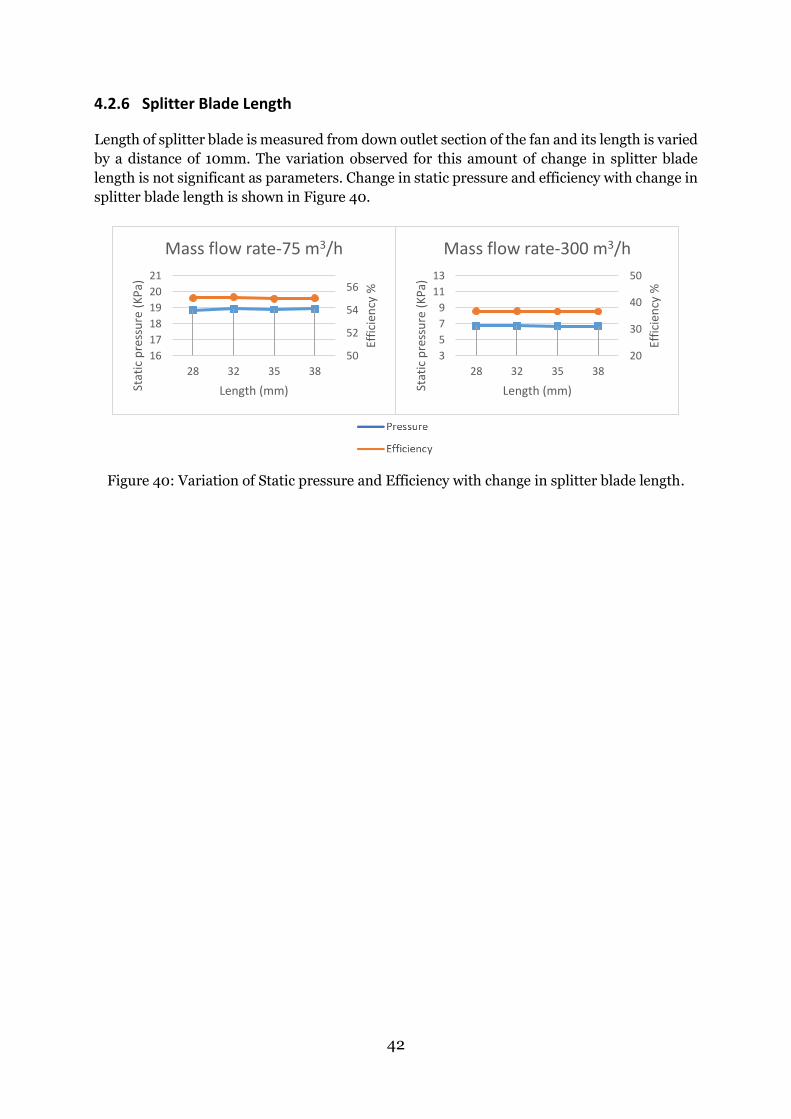
42

4.2.6 Splitter Blade Length

Length of splitter blade is measured from down outlet section of the fan and its length is varied

by a distance of 10mm. The variation observed for this amount of change in splitter blade

length is not significant as parameters. Change in static pressure and efficiency with change in

splitter blade length is shown in Figure 40.

Figure 40: Variation of Static pressure and Efficiency with change in splitter blade length.

50

52

54

56

16

17

18

19

20

21

28 32 35 38Ef

fici

ency

%

Stat

ic p

ress

ure

(K

Pa)

Length (mm)

Mass flow rate-75 m3/h

20

30

40

50

3

5

7

9

11

13

28 32 35 38

Effi

cien

cy %

Stat

ic p

ress

ure

(K

Pa)

Length (mm)

Mass flow rate-300 m3/h

43

5. Discussion

This section discusses the strength and weakness of the method followed during the thesis

work and further on the results from the base model and the parametric study.

5.1 Computational Domain, Geometry and Mesh

As described in section 3.2, the placement of inlet and outlet boundaries far away from focus

object of study ‘fan’ based on literature review in all simulations appears to be sufficient.

Pressure contours on the volute and vertical cross section plane in Figure 19 further justifies

this.

With respect to geometry, only minor changes were made to the models used in simulations

compared to model proposed for manufacture. All the elements in the original model was

retained for the simulation model which is in scope of this work. The secondary flow below the

impeller surface is neglected in the simulations. Considering this could result in decrease of

efficiency and possibly cause convergence issue due to flow complexity expected in that region

due to flow being blocked and impacted by fan rotation. No issues were observed with geometry

used during meshing or when running the simulations at all the mass flow rates.

Automated meshing process with prism layers to capture the boundary layer proves to work

well. The user flexibility is certainly lost with automated meshing process. But for the

complicated impeller geometry and as meshing is quicker with this process, automated

meshing is helpful. Wall functions used in simulations helps in speeding up the meshing

process. Wall function is based on the assumed distribution of velocity, temperature, and

turbulence values in the boundary layer to provide boundary conditions to continuum

equations. The accuracy of these wall functions depends on the assumptions made with respect

to reality in applications. Some accuracy is lost with use of wall functions, but its use can be

justified with many simulations carried out during the work. Considering the resolution of the

mesh, 𝑦+ contour, and with no issues in solution convergence, boundary layer mesh resolution

can be concluded to be satisfactory to meet the requirements of SST k-omega model.

5.3 Choice of Turbulence Model and Physics Used in

Simulations

Steady state RANS, SST k-Omega turbulence model is used in all simulations carried out

during this thesis work. RANS turbulence model does not capture large separations where

there is formation of large and unstable eddies. Hence the simulations are not carried out with

mass flow rate where potential surge and choke conditions where large separation is expected.

Accordingly, simulations here were restricted to mass flow rate from 75 m3/h to 300 m3/h.

44

k- epsilon turbulence models fails to capture separation due to adverse pressure gradients

which is expected in this application. Hence these models are avoided even though it is

computationally less expensive. To simulate the flow at surge and choke conditions it would be

interesting to run simulations with LES or DES models. It would also help to know exact mass

flow rates at which huge separations start to appear that would determine being in the surge

or choke conditions. The results obtained in this work are good with simulations performed

under stable operating range of the fan with RANS model.

During the simulations, walls in the model is treated adiabatic with assumption that there

would be negligible heat transfer from the fluid to the fan and casing material. This assumption

would not be fully appropriate. There would be heat transfer between the fluid and the walls

which makes the efficiency to drop. By applying material properties and treating wall as

diathermal would account into heat transfer between the fluids. This could be done once

material of the fan is selected. But in our case, temperature of the fluid is not significantly high

as in Figure 20 and heat transfer would not be significant. As the performance of the fan is

being analyzed in initial design stage, assumption of adiabatic walls can be considered with

certain loss of accuracy.

5.3 Base Model

The performance curve for the base model as in Figure 17 shows uniform decrease in pressure

with increase in mass flow rate. The aim with the fan performance curve was that pressure

curve should be a constant pressure values at low mass flows and have a sudden bend towards

zero suction pressure at mass flow rate around 300 m3/h. By looking at a typical performance

curves at different RPM speeds in Figure 7, where curves at higher RPM have sudden drop in

pressure, one could relate this sudden bend to the RPM of the fan. Hence, possibly at higher

RPM speeds, it would be easier to get the sharp bend. But also, stable operating range of the

fan could be small which needs to be taken care by adjusting suitable paraments such as inlet

guide vanes which helps in mitigating surge [23].

The results for the base geometry in section 4.1 follow the expected trend in terms of pressure

and efficiency variation with respect to mass flow rates. Static pressure contours show high

suction pressure in pipe inlet at low mass flow and suction pressure decreases with increase in

mass flow. High pressure in scroll outlet region at higher mass flow observed in Figure 19

suggests that clearance gap connecting diffuser section to the scroll housing to be small for this

mass flow which has led to pressure build up in the region. Hence, the clearance gap is varied

during the parametric study and investigated further. High temperature near the outlet of the

pipe compared to inlet region is due to the compression in Figure 20. Air compressed by the

fan causes this increase in temperature on the outlet side. Higher temperature is observed on

temperature contour at low mass flow where significant compression of fluid takes place which

makes sense.

The contour images representing Mach number of the flow in Figure 21 shows some regions

in domain being greater than Mach 0.3 meaning flow has considerable density variations and

compressibility effects are significant. Hence compressibility is considered in this thesis work.

However maximum Mach number reached is well below 0.8 Mach meaning flow has not

entered the transonic region where the shock waves might start to originate which would

45

demand for greater strength of fan material and greater efforts for fan balancing during

rotation.

The contour images of Mach number and TKE represent some distortion of flow in diffuser

section at low mass flow rate. This could be due to improper design of diffuser in that region.

Reason for the flow distortion is further analyzed during the parametric study in next section.

The flow distortion in diffuser section reduces as mass flow increases as seen in the figures 21

and 22.

5.4 Parametric Study

The range of values in which the design parameters were analyzed are chosen so as to be close

to the required performance. Following sub sections discusses the results of each parameter

analyzed in the work.

5.4.1 Fan Diameter

Suction pressure increases as the fan diameter gets bigger in the range as shown in Figure 23

for both high and low mass flow rates. Fluid needs to pass through longer passages between

the blade as the fan diameter gets bigger and hence flow is more compressed leading to higher

suction pressure on inlet side. This can be clearly visualized in Figure 25.

The increase in pressure as fan diameter is increased at both low and high mass flow rates can

be directly related to increase in the passage length as diameter increases where the fluid gets

compressed. This results in higher suction pressure at the inlet pipe side. The efficiency

decreases as the fan diameter is increased for low mass flow rate. Fan requires higher torque

when the diameter gets bigger and the compressed fluid gets separated at the fan blade tip due

to presence of adverse pressure gradient as at outlet part, fluid at higher pressure is present.

This leads to higher entropy of the flow as flow exits the fan into diffuser as visualized in Figure

24. Higher the entropy of the flow, more is the flow mixing, resulting in efficiency reduction.

However, at high mass flow rates, efficiency increases as the fan diameter gets bigger. At high

flow rates, blockages withing the fan and at the outlet section can be expected. With bigger

diameter, fan is able to displace the flow without creating blockages as in Figure 25. This leads

to increase in efficiency as fan diameter gets bigger at higher mass flow rate.

5.4.2 Outlet Blade angle

Suction pressure decreases as the outlet blade angle increases at both high and low mass flow

rates as seen from Figure 27. Blade is twisted more at higher outlet blade angles. More the

twist, air seems to find it difficult to follow the twisted channel and hence lose out on the

compression leading to lower suction pressure.

Greater efficiency is observed at higher outlet angles (high twist) at low mass flow rate. Greater

the twist, the flow seems to be more attached to the blades in the outlet region of the fan and

hence less mixing of the flow leading to lower entropy at 75 m3/h flow rate as in Figure 28. The

46

flow distorted at lesser outlet angle blades can be visualized in velocity contour in diffuser

section as in Figure 29 which explains the efficiency trend at low mass flow rate.

Velocity in the scroll outlet section is not uniform as seen in Figure 29. Velocity of flow is high

where there is less internal flow area and velocity falls in regions where internal flow area

becomes large. Sudden changes in velocity is due to non-uniform changes in internal flow area

inside scroll housing.

Pressure contour in Figure 30 shows the greater possible impact of adverse pressure gradient

for the high twist blades. This could cause the blockage for the flow in the fan diffuser section

at high mass flow rate. Hence, lower the twist, the better efficiency at higher mass flow rate.

As seen in Figure 27, highest static suction pressure obtained is around 19 kPa for the lowest

outlet blade angle. It could be interesting to see further reduce the outlet blade angle and see

if the pressure continues to increase. This is important as the required suction static pressure

at 75 m3/h was 20 kPa. On the other hand, at mass flow rate of 300 m3/h, decreasing the outlet

blade angle is resulting in higher static suction pressure which is not required. Hence an

optimal blade angle needs to be determined to satisfy suction static pressure requirements at

both the mass flow rates.

5.4.3 Number of impeller blades

No high variation in pressure and efficiency is observed from this parametric study as in Figure

31. Slight variations in pressure and efficiency at low and high mass flow rate can be attributed

to flow attachment and clearance for the flow, respectively. At low mass flow rate, the distortion

in the flow is high in the diffuser region as number of blades gets less as in Figure 32. This

distortion of flow would depend on how the flow is attached in the fan region. More the number

of blades, more possibility for the flow to be attached. This causes less separation leading to

less flow distortion as the flow exits from fan into the diffuser region. Variation in velocity due

seen in Figure 32 can be attributed to non-uniform changes in internal flow area inside the

scroll housing as explained in above section.

At the higher mass flow rate, greater the number of blades, more obstruction it causes for the

flow. More number of blades causes blockage as in Figure 33. leading to backflow and hence

reduction in efficiency.

5.4.4 Curvature Radius

As radius of the curve connecting the inlet section to the outlet section of the fan increases,

fluid has to travel comparatively through a shorter distance and hence flow is compressed to

lower extent resulting in lower suction pressure at low and high mass flow rates.

At low mass flow rate, fluid passing through higher radius curve and shorter distance

encounters less turbulence as the flow passes into diffuser region. As the curvature decreases,

more area is available for the flow in the fan region hence higher probability for flow to get

distorted and become turbulent which is confirmed by the TKE plot in Figure 36. Hence higher

curvature radius results in higher efficiency.

47

The fluid at high mass flow rate encounters blockage as the radius of the curve increases.

Blockage is due to the distance between the stationary casing and the curve decreases which in

turn reduces the area available for flow in the fan region. Reduction in area increases the

turbulence in the flow as it enters the diffuser region. This leads to decrease in efficiency as

radius of the curve increases.

As seen in Figure 35, highest static suction pressure obtained is around 19 kPa for the lowest

curvature radius. It could be interesting to see further reduce the curvature radius and see if

the pressure continues to increase. This is important as the required suction static pressure at

75 m3/h was 20 kPa. On the other hand, at mass flow rate of 300 m3/h, decreasing the

curvature radius is resulting in higher static suction pressure which is not required. Hence an

optimal curvature radius needs to be determined to satisfy suction static pressure

requirements at both the mass flow rates.

5.4.5 Diffuser exit length

Suction pressure at low mass flow undergoes less change when the exit length at the diffuser is

changed. Increase in suction pressure can be observed as the diffuser exit length increases from

the Figure 38.

Efficiency decreases as the exit length of the diffuser is increased. Backflow is observed in

diffuser region as the exit length increases as seen in Figure 39. The adverse pressure gradient

causes this backflow making fan to work harder to push the fluid towards the outlet.

However, efficiency increases as exit length increases at higher mass flow. This can be directly

related to the blockage of the high mass flow. Greater the exit length, more area is available for

the high mass flow without any disturbance in the passage leading to greater efficiency.

5.4.6 Length of Splitter Blade

Effect of splitter blade length is less on variation of static pressure and efficiency at both low

and high mass flow rates as seen in Figure 40. This could be related as effect of number of

blades also had less impact on the variation of static pressure and efficiency. Hence more

detailed analysis is not conducted in this thesis work.

48

6. Conclusions

The base model designed during this thesis work gave performance close to the required values

in terms of air flow rate and static pressure. It is evident from the results that general

aerodynamics of the base model developed is appreciated more. No distinctive flow patterns

were observed inside the fan and its housing. Another result worth noting is that the suction

static pressure decreased as air flow rate increased. Flow rates at which surge, and choke

conditions appear have not been simulated during this work due to limitations with turbulence

modelling in RANS.

Parametric analysis conducted on few design variables gave good results. In the range in which

each parameter was tested, variation with fan diameter, blade outlet angle, radius of the curve

connecting inlet to outlet section of the fan and diffuser exit length produced greater variance

in static pressure and efficiency compared to parameters such as number of impeller blades

and splitter blade length. Number of blades and splitter length blade can be varied further to

see larger variation in pressure and efficiency. To get a broader view on behavior of the fan

performance, the range in which all parameters were tested could have been extended.

For further understanding of the fan design, analyzing other parameters would be interesting.

To improve the efficiency at low mass flow rates, analysis on inlet guide vanes will be useful.

To get the required flow, parameters such as blade height at the fan outlet and inlet blade angle

could prove to be useful. To get a sudden drop in the pressure curve, operating at higher RPM

speeds and reducing the fan diameter could be investigated. Velocity contours from the

parametric study of blade outlet angle and number of impeller blades show non-uniform

velocity patterns in the scroll outlet. Hence further analysis and improvement of scroll housing

is necessary. As a next step, an algorithm can be developed and used to optimize the design

parameters which have impact on performance to get the best suitable fan capable of giving

performance very close to the requirements. Considerations of dimensional constraints,

machining cost and material for the fan would be challenging during optimization.

49

References

[1] Kennedy D (2003). Process machinery: Advanced industrial vacuum cleaning systems increase productivity and improve safety. Rubber World 227(5):22–23. [2] H K Versteeg, W Malalasekera. An Introduction to Computational Fluid Dynamics -THE FINITE VOLUME METHOD. 2nd ed. Pearson; 2007. [3] Schwind R, Abdallah S (2015), A Look at Compressor Impeller Technologies for Turbochargers Focusing on Surge Mitigation. Global J Technol Optim 6: 185. doi:10.4172/2229-8711.1000185 [4] Nassar A, Hagpurwala QH, Reddy KB (2006). Design and CFD investigation of centrifugal compressor for turbocharger and parametric study on splitter blades.Sas Tech 2: 35-41. [5] D. Maestre, R. Ramirez, W. Oliveira, T. Arispe. Methodology for a Numerical Analysis of the Aerodynamic Performance of a Centrifugal Fan Trough Computational Fluid Dynamics (CFD), COBEM, 2019 [6] Anagnostopoulos, John. (2006). CFD Analysis and Design Effects in a Radial Pump Impeller. WSEAS Trans Fluid Mech. 1. [7] Després G, Ngo Boum G, Leboeuf F, Chalet D, Chesse P, Lefebvre A, 2013. Simulation of near surge instabilities onset in a turbocharger compressor. Proceedings of the Institution of Mechanical Engineers, Part A: Journal of Power and Energy 227, 6 665-673. [8] Fjällman J, 2014. Large eddy simulation of complex fows in IC-engine's exhaust manifold and turbine. Doctoral Thesis, Royal Institute of Technology Stockholm 2014 [9] Yu, Zhao & Li, Song & He, Wenqi & Wang, Weixiong & Huang, Dongtao & Zhu, Zhichi. (2005). Numerical Simulation of Flow Field for a Whole Centrifugal Fan and Analysis of the Effects of Blade Inlet Angle and Impeller Gap. HVAC&R Research. 11. 263-283. 10.1080/10789669.2005.10391137. [10] Celik IB, Ghia U, Roache PJ et al. 2008. Procedure for estimation and reporting of uncertainty due to discretization in CFD applications. J. Fluids Eng., 130 (7) [11] Philip J. O’ Keefe, PE, MLE 2018. Centrifugal Pump Impeller Action, Engineering Expert

Witness Blog; http://www.engineeringexpert.net/Engineering-Expert-Witness-Blog/tag/impeller-blades

[12] James M. Sorokes, 2013, Selecting a Centrifugal Compressor, American Institute of Chemical Engineers (AIChE) and Dresser-Rand. [13] Power Zone Equipment, INC., Compressors, Fans and Blowers, https://www.powerzone.com/resources/glossary/compressorsfansblowers

[14] Design Spark; Fan types- Choosing centrifugal fan; https://www.rs-online.com/designspark/fan-types-why-choose-a-forward-curved-centrifugal-fan#:~:text=The%20difference%20in%20flow%20direction,the%20circumference%20of%20the%20fan.

50

[15] Fluid machine lecture notes; http://www.fkm.utm.my/~syahruls/3-teaching/2-fluid-II/fluid-II-enote/31-pump.pdf [16] Badarch, Ayurzana. (2015). Hydropower scheme to strengthen CES of Mongolia. 10.13140/RG.2.1.2314.6489. [17] Ander Eza. (2015). Flow simulations with relevance to a centrifugal compressor and the

effect of the inlet geometry. Master Thesis –KTH university.

[18] Siemens. Simcenter STARCCM+ Theory; ///share/apps/cd-adapco/RHEL5/ v14.06.012/STAR-CCM+14.06.012/doc/en/online/index.html#page/ STARCCMP%2FGUID-

2F109228-1392-4437-8E6C-9FA99865011F.html%23. [19] Richardson, L. F., 1910, “The Approximate Arithmetical Solution by Finite Differences of Physical Problems Involving Differential Equations, With an Application to the Stresses in a

Masonary Dam,” Philos. Trans. R. Soc. London, Ser. A0962 8428, 210, pp. 307–357

[20] Richardson, L. F., and Gaunt, J. A., 1927, “The Deferred Approach to the Limit,” Philos. Trans. R. Soc. London, Ser. A0962-8428, 226, pp. 299–361.

[21] Bogdanovic-Jovanovic, Jasmina & Bogdanović, Božidar & Spasić, Živan. (2019). Centrifugal Fans with Backward-curved and Forward-curved Blades.

[22] NMB ; Fan efficiency; The Importance of fan efficiency;

https://www.newark.com/wcsstore/ExtendedSitesCatalogAssetStore/cms/asset/images/americas/common/storefront/nmb-technologies/7931_Fan-Efficiency-an-Increasingly-Important-Selection-Criteria.pdf [23] Mohtar, Hani. (2010). INCREASING SURGE MARGIN OF TURBOCHARGER CENTRIFUGAL COMPRESSOR AUTOMOTIVE APPLICATION. [24] Epple, Philipp & Durst, F. & Delgado, Antonio. (2010). A theoretical derivation of the Cordier diagram for turbomachines. Proceedings of The Institution of Mechanical Engineers Part C-journal of Mechanical Engineering Science - PROC INST MECH ENG C-J MECH E. 1. 1-15. 10.1243/09544062JMES228